Fast Cross-Validation for Incremental Learning

Abstract

Cross-validation (CV) is one of the main tools for performance estimation and parameter tuning in machine learning. The general recipe for computing CV estimate is to run a learning algorithm separately for each CV fold, a computationally expensive process. In this paper, we propose a new approach to reduce the computational burden of CV-based performance estimation. As opposed to all previous attempts, which are specific to a particular learning model or problem domain, we propose a general method applicable to a large class of incremental learning algorithms, which are uniquely fitted to big data problems. In particular, our method applies to a wide range of supervised and unsupervised learning tasks with different performance criteria, as long as the base learning algorithm is incremental. We show that the running time of the algorithm scales logarithmically, rather than linearly, in the number of CV folds. Furthermore, the algorithm has favorable properties for parallel and distributed implementation. Experiments with state-of-the-art incremental learning algorithms confirm the practicality of the proposed method.

1 Introduction

Estimating generalization performance is a core task in machine learning. Often, such an estimate is computed using $k$-fold cross-validation ($k$-CV): the dataset is partitioned into $k$ subsets of approximately equal size, and each subset is used to evaluate a model trained on the $k-1$ other subsets to produce a numerical score; the $k$-CV performance estimate is then obtained as the average of the obtained scores.

A significant drawback of $k$-CV is its heavy computational cost. The standard method for computing a $k$-CV estimate is to train $k$ separate models independently, one for each fold, requiring (roughly) $k$-times the work of training a single model. The extra computational cost imposed by $k$-CV is especially high for leave-one-out CV (LOOCV), a popular variant, where the number of folds equals the number of samples in the dataset. The increased computational requirements may become a major problem, especially when CV is used for tuning hyper-parameters of learning algorithms in a grid search, in which case one $k$-CV session needs to be run for every combination of hyper-parameters, dramatically increasing the computational cost even when the number of hyper parameters is small.

To avoid the added cost, much previous research went into studying the efficient calculation of the CV estimate (exact or approximate). However, previous work has been concerned with special models and problems: With the exception of Izbicki Izbicki (2013), these methods are typically limited to linear prediction with the squared loss and to kernel methods with various loss functions, including twice-differentiable losses and the hinge loss (see Section 1.1 for details). In these works, the training time of the underlying learning algorithm is $\Theta(n^{3})$, where $n$ is the size of the dataset, and the main result states that the CV-estimate (including LOOCV estimates) is yet computable in $O(n^{3})$ time. Finally, Izbicki Izbicki (2013) gives a very efficient solution (with $O(n+k)$ computational complexity) for the restrictive case when two models trained on any two datasets can be combined, in constant time, into a single model that is trained on the union of the datasets.

Although these results are appealing, they are limited to methods and problems with specific features. In particular, they are unsuitable for big data problems where the only practical methods are incremental and run in linear, or even sub-linear time Shalev-Shwartz et al. (2011); Clarkson et al. (2012). In this paper, we show that CV calculation can be done efficiently for incremental learning algorithms. In Section 3, we present a method that, under mild, natural conditions, speeds up the calculation of the $k$-CV estimate for incremental learning algorithms, in the general learning setting explained in Section 2 (covering a wide range of supervised and unsupervised learning problems), and for arbitrary performance measures. The proposed method, TreeCV, exploits the fact that incremental learning algorithms do not need to be fed with the whole dataset at once, but instead learn from whatever data they are provided with and later update their models when more data arrives, without the need to be trained on the whole dataset from scratch. As we will show in Section 3.1, TreeCV computes a guaranteed-precision approximation of the CV estimate when the algorithms produce stable models. We present several implementation details and analyze the time and space complexity of TreeCV in Section 4. In particular, we show that its computation time is only $O(\log k)$-times bigger than the time required to train a single model, which is a major improvement compared to the $k$-times increase required for a naive computation of the CV estimate. Finally, Section 5 presents experimental results, which confirm the efficiency of the proposed algorithm.

1.1 Related Work

Various methods, often specialized to specific learning settings, have been proposed to speed up the computation of the $k$-CV estimate. Most frequently, efficient $k$-CV computation methods are specialized to the regularized least-squares (RLS) learning settings (with squared-RKHS-norm regularization). In particular, the generalized cross-validation method Golub et al. (1979); Wahba (1990) computes the LOOCV estimate in $O(n^{2})$ time for a dataset of size $n$ from the solution of the RLS problem over the whole dataset; this is generalized to $k$-CV calculation in $O(n^{3}/k)$ time by Pahikkala et al. Pahikkala et al. (2006). In the special case of least-squares support vector machines (LSSVMs), Cawley Cawley (2006) shows that LOOCV can be computed in $O(n)$ time using a Cholesky factorization (again, after obtaining the solution of the RLS problem). It should be noted that all of the aforementioned methods use the inverse (or some factorization) of a special matrix (called the influence matrix) in their calculation; the aforementioned running times are therefore based on the assumption that this inverse is available (usually as a by-product of solving the RLS problem, computed in $\Omega(n^{3})$ time).

A related idea for approximating the LOOCV estimate is using the notion of influence functions, which measure the effect of adding an infinitesimal single point of probability mass to a distribution. Using this notion, Debruyne et al. Debruyne et al. (2008) propose to approximate the LOOCV estimate for kernel-based regression algorithms that use any twice-differentiable loss function. Liu et al. Liu et al. (2014) use Bouligand influence functions Christmann and Messem (2008), a generalized notion of influence functions for arbitrary distributions, in order to calculate the $k$-CV estimate for kernel methods and twice-differentiable loss functions. Again, these methods need an existing model trained on the whole dataset, and require $\Omega(n^{3})$ running time.

A notable exception to the square-loss/differentiable loss requirement is the work of Cauwenberghs and Poggio Cauwenberghs and Poggio (2001). They propose an incremental training method for support-vector classification (with the hinge loss), and show how to revert the incremental algorithm to “unlearn” data points and obtain the LOOCV estimate. The LOOCV estimate is obtained in time similar to that of a single training by the same incremental algorithm, which is $\Omega(n^{3})$ in the worst case.

Closest to our approach is the recent work of Izbicki Izbicki (2013): assuming that two models trained on any two separate datasets can be combined, in constant time, to a single model that is exactly the same as if the model was trained on the union of the datasets, Izbicki Izbicki (2013) can compute the $k$-CV estimate in $O(n+k)$ time. However his assumption is very restrictive and applies only to simple methods, such as Bayesian classification. In contrast, roughly, we only assume that a model can be updated efficiently with new data (as opposed to combining the existing model and a model trained on the new data in constant time), and we only require that models trained with permutations of the data be sufficiently similar, not exactly the same.

Note that the CV estimate depends on the specific partitioning of the data on which it is calculated. To reduce the variance due to different partitionings, the $k$-CV score can be averaged over multiple random partitionings. For LSSVMs, An et al. An et al. (2007) propose a method to efficiently compute the CV score for multiple partitionings, resulting in a total running time of $O(L(n-b)^{3})$, where $L$ is the number of different partitionings and $b$ is the number of data points in each test set. In the case when all possible partitionings of the dataset are used, the complete CV (CCV) score is obtained. Mullin and Sukthankar Mullin and Sukthankar (2000) study efficient computation of CCV for nearest-neighbor-based methods; their method runs in time $O(n^{2}k+n^{2}\log(n))$.

2 Problem Definition

We consider a general setting that encompasses a wide range of supervised and unsupervised learning scenarios (see Table 1 for a few examples). In this setting, we are given a dataset $\{z_{1},z_{2},\ldots,z_{n}\}$, where each data point $z_{i}=(x_{i},y_{i})$ consists of an input $x_{i}\in\mathcal{X}$ and an outcome $y_{i}\in\mathcal{Y}$, for some given sets $\mathcal{X}$ and $\mathcal{Y}$. For example, we might have $\mathcal{X}\subset\mathbb{R}^{d},d\geq 1$, with $\mathcal{Y}=\{+1,-1\}$ in binary classification and $\mathcal{Y}\subset\mathbb{R}$ in regression; for unsupervised learning, $\mathcal{Y}$ is a singleton: $\mathcal{Y}=\{{\textsc{NoLabel}}\}$. We define a model as a function $f:\mathcal{X}\to\mathcal{P}$ that, given an input $x\in\mathcal{X}$, makes a prediction, $f(x)\in\mathcal{P}$, where $\mathcal{P}$ is a given set (for example, $\mathcal{P}=\{+1,-1\}$ in binary classification: the model predicts which class the given input belongs to). Note that the prediction set need not be the same as the outcome set, particularly for unsupervised learning tasks. The quality of a prediction is assessed by a performance measure (or loss function) $\ell:\mathcal{P}\times\mathcal{X}\times\mathcal{Y}\to\mathbb{R}$ that assigns a scalar value $\ell(p,x,y)$ to the prediction $p$ for the pair $(x,y)$; for example, $\ell(p,x,y)=\mathbb{I}\left\{p\neq y\right\}$ for the prediction error (misclassification rate) in binary classification (where $\mathbb{I}\left\{E\right\}$ denotes the indicator function of an event $E$).

Setting $\mathcal{X}$ $\mathcal{Y}$ $\mathcal{P}$ $\ell(f(x),x,y)$ Classification $\mathbb{R}^{d}$ $\{+1,-1\}$ $\{+1,-1\}$ $\mathbb{I}\left\{f(x)\neq y\right\}$ Regression $\mathbb{R}^{d}$ $\mathbb{R}$ $\mathbb{R}$ $(f(x)-y)^{2}$ $K$-means clustering $\mathbb{R}^{d}$ $\{{\textsc{NoLabel}}\}$ $\{c_{1},c_{2},\ldots,c_{K}\}\subset\mathbb{R}^{d}$ $\|x-f(x)\|^{2}$ Density estimation $\mathbb{R}^{d}$ $\{\textsc{NoLabel}\}$ $\{f:f\textnormal{ is a density}\}$ $-\log(f(x))$

Table 1: Instances of the general learning problem considered in the paper. In $K$-means clustering, $c_{j}$ denotes the center of the $j$th cluster.

Next, we define the notion of an incremental learning algorithm. Informally, an incremental learning algorithm is a procedure that, given a model learned from previous data points and a new dataset, updates the model to accommodate the new dataset at the fraction of the cost of training the model on the whole data from scratch. Formally, let $\mathcal{M}\subseteq\left\{f:\mathcal{X}\to\mathcal{P}\right\}$ be a set of models, and define $\mathcal{Z}^{*}$ to be the set of all possible datasets of all possible sizes. Disregarding computation for now, an incremental learning algorithm is a mapping $\mathcal{L}:\left(\mathcal{M}\cup\{\emptyset\}\right)\times\mathcal{Z}^{*}\to\mathcal{M}$ that, given a model $f$ from $\mathcal{M}$ (or $\emptyset$ when a model does not exist yet) and a dataset $Z^{\prime}=(z^{\prime}_{1},z^{\prime}_{2},\ldots,z^{\prime}_{m})$, returns an “updated” model $f^{\prime}=\mathcal{L}(f,Z^{\prime})$. To capture often needed internal states (e.g., to store learning rates), we allow the “padding” of the models in $\mathcal{M}$ with extra information as necessary, while still viewing the models as $\mathcal{X}\to\mathcal{P}$ maps when convenient. Above, $f$ is usually the result of a previous invocation of $\mathcal{L}$ on another dataset $Z\in\mathcal{Z}^{*}$. In particular, $\mathcal{L}(\emptyset,Z)$ learns a model from scratch using the dataset $Z$. An important class of incremental algorithms are online algorithms, which update the model one data point at a time: to update $f$ with $Z^{\prime}$, these algorithms make $m$ consecutive calls to $\mathcal{L}$, where each call updates the latest model with the next remaining data point according to a random ordering of the points in $Z^{\prime}$.

In the rest of this paper, we consider an incremental learning algorithm $\mathcal{L}$, and a fixed, given partitioning of the dataset $\{z_{1},z_{2},\ldots,z_{n}\}$ into $k$ subsets (“chunks”) $Z_{1},Z_{2},\ldots,Z_{k}$. We use $f_{i}=\mathcal{L}(\emptyset,Z\setminus Z_{i})$ to denote the model learned from all the chunks except $Z_{i}$. Thus, the $k$-CV estimate of the generalization performance of $\mathcal{L}$, denoted $R_{k\textnormal{-CV}}$, is given by

$$R_{k\textnormal{-CV}}=\dfrac{1}{k}\sum_{i=1}^{k}R_{i},$$

where $R_{i}=\frac{1}{|Z_{i}|}\sum_{(x,y)\in Z_{i}}\ell(f_{i}(x),x,y),i=1,2,\ldots,k,$ is the performance of the model $f_{i}$ evaluated on $Z_{i}$. The LOOCV estimate $R_{n\textnormal{-CV}}$ is obtained when $k=n$.

3 Recursive Cross-Validation

Our algorithm builds on the observation that for every $i$ and $j$, $1\leq i<j\leq k$, the training sets $Z\setminus Z_{i}$ and $Z\setminus Z_{j}$ are almost identical, except for the two chunks $Z_{i}$ and $Z_{j}$ that are held out for testing from one set but not the other. The naive $k$-CV calculation method ignores this fact, potentially wasting computational resources. When using an incremental learning algorithm, we may be able to exploit this redundancy: we can first learn a model only from the examples shared between the two training sets, and then “increment” the differences into two different copies of the model learned. When the extra cost of saving and restoring a model required by this approach is comparable to learning a model from scratch, then this approach may result in a considerable speedup.

Algorithm 1 $\textsc{TreeCV}\left(s,e,\hat{f}_{s..e}\right)$

  input: indices $s$ and $e$, and the model $\hat{f}_{s..e}$ trained so far.

  if $e=s$ then

     $\hat{R}_{s}\leftarrow\frac{1}{|Z_{s}|}\sum_{(x,y)\in Z_{s}}\ell\left(\hat{f}_{s..e}(x),x,y\right).$

     return $\frac{1}{k}\hat{R}_{s}$.

  else

     Let $m\leftarrow\left\lfloor\frac{s+e}{2}\right\rfloor$.

     Update the model with the chunks $Z_{m+1},\ldots,Z_{e}$ to get $\hat{f}_{s..m}=\mathcal{L}(\hat{f}_{s..e},Z_{m+1},\ldots,Z_{e})$.

     Let $r\leftarrow\textsc{{TreeCV}}\left(s,m,\hat{f}_{s..m}\right)$.

     Update the model with the chunks $Z_{s},\ldots,Z_{m}$ to get $\hat{f}_{m+1..e}=\mathcal{L}(\hat{f}_{s..e},Z_{s},\ldots,Z_{m})$.

     Let $r\leftarrow r+\textsc{{TreeCV}}\left(m+1,e,\hat{f}_{m+1..e}\right)$.

     return $r$.

  end if

To exploit the aforementioned redundancy in training all $k$ models at the same time, we organize the $k$-CV computation process in a tree structure. The resulting recursive procedure, $\textsc{{TreeCV}}(s,e,\hat{f}_{s..e})$, shown in Algorithm 1, receives two indices $s$ and $e$, $1\leq s\leq e\leq k$, and a model $\hat{f}_{s..e}$ that is trained on all chunks except $Z_{s},Z_{s+1},\ldots,Z_{e}$, and returns $(1/k)\sum_{i=s}^{e}\hat{R}_{i}$, the normalized sum of the performance scores $\hat{R}_{i},i=s,\ldots,e,$ corresponding to testing $\hat{f}_{i..i}$, the model trained on $Z\setminus Z_{i}$, on the chunk $Z_{i}$, for $i=s,\ldots,e$. TreeCV divides the hold-out chunks into two groups $Z_{s},Z_{s+1},\ldots,Z_{m}$ and $Z_{m+1},\ldots Z_{e}$, where $m=\left\lfloor\frac{s+e}{2}\right\rfloor$ is the mid-point, and obtains the test performance scores for the two groups separately by recursively calling itself. More precisely, TreeCV first updates the model by training it on the second group of chunks, $Z_{m+1},\ldots,Z_{e}$, resulting in the model $\hat{f}_{s..m}$, and makes a recursive call $\textsc{{TreeCV}}(s,m,\hat{f}_{s..m})$ to get $(1/k)\sum_{i=s}^{m}\hat{R}_{i}$. Then, it repeats the same procedure for the other group of chunks: starting from the original model $\hat{f}_{s..e}$ it had received, it updates the model, this time using the first group of the remaining chunks, $Z_{s},\ldots,Z_{m}$, that were previously held out, and calls $\textsc{{TreeCV}}(m+1,e,\hat{f}_{m+1..e})$ to get $(1/k)\sum_{i=m+1}^{e}\hat{R}_{i}$ (for the second group of chunks). The recursion stops when there is only one hold-out chunk ($s=e$), in which case the performance score $\hat{R}_{s}$ of the model $\hat{f}_{s..s}$ (which is now trained on all the chunks except for $Z_{s}$) is directly calculated and returned. Calling $\textsc{{TreeCV}}(1,n,\emptyset)$ calculates $\hat{R}_{k\textnormal{-CV}}=\frac{1}{k}\sum_{i=1}^{k}\hat{R}_{i}$. Figure 1 shows an example of the recursive call tree underlying a run of the algorithm calculating the LOOCV estimate on a dataset of four data points. Note that the tree structure imposes a new order of feeding the chunks to the learning algorithm, e.g., $z_{3}$ and $z_{4}$ are learned before $z_{2}$ in the first branch of the tree.

Figure 1: An example run of TreeCV on a dataset of size four, calculating the LOOCV estimate.

3.1 Accuracy of TreeCV

To simplify the analysis, in this section and the next, we assume that each chunk is of the same size, that is $n=kb$ for some integer $b\geq 1$.

Note that the models $\hat{f}_{s..s}$ used in computing $\hat{R}_{s}$ are learned incrementally. If the learning algorithm learns the same model no matter whether it is given the chunks all at once or gradually, then $\hat{f}_{s..s}$ is the same as the model $f_{s}$ used in the definition of $R_{k\textnormal{-CV}}$, and $R_{k\textnormal{-CV}}=\hat{R}_{k\textnormal{-CV}}$. If this assumption does not hold, then $\hat{R}_{k\textnormal{-CV}}$ is still close to $R_{k\textnormal{-CV}}$ as long as the models $\hat{f}_{s..s}$ are sufficiently similar to their corresponding models $f_{s}$. In the rest of this section, we formalize this assertion.

First, we define the notion of stability for an incremental learning algorithm. Intuitively, an incremental learning algorithm is stable if the performance of the models are nearly the same no matter whether they are learned incrementally or in batch. Formally, suppose that a dataset $\{z_{1},\ldots,z_{n}\}$ is partitioned into $l+1$ nonempty chunks $Z^{\textnormal{test}}$ and $Z^{\textnormal{train}}_{1},\ldots,Z^{\textnormal{train}}_{l}$, and we are using $Z^{\textnormal{test}}$ as the test data and the chunks $Z^{\textnormal{train}}_{1},\ldots,Z^{\textnormal{train}}_{l}$ as the training data. Let $f^{\textnormal{batch}}=\mathcal{L}(\emptyset,Z^{\textnormal{train}}_{1}\cup\ldots\cup Z^{\textnormal{train}}_{l})$ denote the model learned from the training data when provided all at the same time, and let

$$f^{\textnormal{inc}}=\mathcal{L}\Bigg{(}\mathcal{L}\bigg{(}\ldots\Big{(}\mathcal{L}(\emptyset,Z^{\textnormal{train}}_{1}),Z^{\textnormal{train}}_{2}\Big{)},\ldots,Z^{\textnormal{train}}_{l-1}\bigg{)},Z^{\textnormal{train}}_{l}\Bigg{)}$$

denote the model learned from the same chunks when they are provided incrementally to $\mathcal{L}$. Let $R^{\textnormal{test}}(f)=\frac{1}{|Z^{\textnormal{test}}|}\sum_{(x,y)\in Z^{\textnormal{test}}}\ell\left(f(x),x,y\right)$ denote the performance of a model $f$ on the test data $Z^{\textnormal{test}}$.

Definition 1 (Incremental stability).

The algorithm $\mathcal{L}$ is $g$-incrementally stable for a function $g:\mathbb{N}\times\mathbb{N}\to\mathbb{R}$ if, for any dataset $\{z_{1},z_{2},\ldots,z_{n}\}$, $b<n$, and partition $Z^{\textnormal{test}},Z^{\textnormal{train}}_{1},\ldots,Z^{\textnormal{train}}_{l}$ with nonempty cells $Z^{\textnormal{train}}_{i},1\leq i\leq l$ and $|Z^{\textnormal{test}}|=b$, the test performance of the models $f^{\textnormal{batch}}$ and $f^{\textnormal{inc}}$ defined above satisfy

$$\left|R^{\textnormal{test}}(f^{\textnormal{inc}})-R^{\textnormal{test}}(f^{\textnormal{batch}})\right|\leq g\left(n-b,b\right).$$

If the data $\{z_{1},\ldots,z_{n}\}$ is drawn independently from the same distribution $\mathcal{D}$ over $\mathcal{X}\times\mathcal{Y}$ and/or the learning algoritm $\mathcal{L}$ is randomized, we say that $\mathcal{L}$ is $g$-incrementally stable in expectation if

$$\left|\mathbb{E}\!\left[R^{\textnormal{test}}(f^{\textnormal{inc}})\right]-\mathbb{E}\!\left[R^{\textnormal{test}}(f^{\textnormal{batch}})\right]\right|\leq g\left(n-b,b\right)$$

for all partitions selected independently of the data and the randomization of $\mathcal{L}$.

The following statement is an immediate consequence of the above definition:

Theorem 1.

Suppose $n=bk$ for some integer $b\geq 1$ and that algorithm $\mathcal{L}$ is $g$-incrementally stable. Then,

$$\left|\hat{R}_{k\textnormal{-CV}}-R_{k\textnormal{-CV}}\right|\leq g\left(n-b,b\right).$$

If $\mathcal{L}$ is $g$-incrementally stable in expectation then

$$\left|\mathbb{E}\!\left[\hat{R}_{k\textnormal{-CV}}\right]-\mathbb{E}\!\left[R_{k\textnormal{-CV}}\right]\right|\leq g\left(n^{\prime},b\right).$$

Proof.

We prove the first statement only, the proof of the second part is essentially identical. Recall that $Z_{j},j=1,2,\dots,k$ denote the chunks used for cross-validation. Fix $i$ and let $l=\left\lceil\log k\right\rceil$. Let $Z^{\textnormal{test}}=Z_{i}$ and $Z^{\textnormal{train}}_{j},j=1\ldots l$, denote the union of the chunks used for training at depth $j$ of the recursion branch ending with the computation of $\hat{R}_{i}$. Then, by definition, $\hat{R}_{i}=R^{\textnormal{test}}(f^{\textnormal{inc}})$ and $R_{i}=R^{\textnormal{test}}(f^{\textnormal{batch}})$. Therefore, $|\hat{R}_{i}-R_{i}|\leq g\left(n-b,b\right)$, and the statement follows since $\hat{R}_{k\textnormal{-CV}}$ and $R_{k\textnormal{-CV}}$ are defined as the averages of the $\hat{R}_{i}$ and $R_{i}$, respectively. ∎

It is then easy to see that incremental learning methods with a bound on their excess risk are incrementally stable in expectation.

Theorem 2.

Suppose the data $\{z_{1},\ldots,z_{n}\}$ is drawn independently from the same distribution $\mathcal{D}$ over $\mathcal{X}\times\mathcal{Y}$. Let $(X,Y)\in\mathcal{X}\times\mathcal{Y}$ be drawn from $\mathcal{D}$ independently of the data and let $f^{*}\in\operatorname*{arg\,min}_{f\in\mathcal{M}}\mathbb{E}\!\left[\ell(f(X),X,Y)\right]$ denote a model in $\mathcal{M}$ with minimum expected loss. Assume there exist upper bounds $m^{\textnormal{batch}}(n-b)$ and $m^{\textnormal{inc}}(n-b)$ on the excess risks of $f^{\textnormal{batch}}$ and $f^{\textnormal{inc}}$, trained on $n^{\prime}=n-b$ data points, such that

$$\mathbb{E}\!\left[\ell(f^{\textnormal{batch}}(X),X,Y)-\ell(f^{*}(X),X,Y)\right]\leq m^{\textnormal{batch}}(n^{\prime})$$

and

$$\mathbb{E}\!\left[\ell(f^{\textnormal{inc}}(X),X,Y)-\ell(f^{*}(X),X,Y)\right]\leq m^{\textnormal{inc}}(n^{\prime})$$

for all $n$ and for every partitioning of the dataset that is independent of the data, $(X,Y)$, and the randomization of $\mathcal{L}$. Then $\mathcal{L}$ is incrementally stable in expectation w.r.t. the loss function $\ell$, with $g(n^{\prime},b)=\max\{m^{\textnormal{batch}}(n^{\prime}),m^{\textnormal{inc}}(n^{\prime})\}$.

Proof.

Since the data points in the sets $Z^{\textnormal{train}}_{1},\ldots,Z^{\textnormal{train}}_{l}$ and $Z^{\textnormal{test}}$ are independent, $f^{\textnormal{batch}}$ and $f^{\textnormal{inc}}$ are both independent of $Z^{\textnormal{test}}$. Hence, $\mathbb{E}\!\left[R^{\textnormal{test}}(f^{\textnormal{batch}})\right]=\mathbb{E}\!\left[\ell\left(f^{\textnormal{batch}}(X),X,Y\right)\right]$ and $\mathbb{E}\!\left[R^{\textnormal{test}}(f^{\textnormal{inc}})\right]=\mathbb{E}\!\left[\ell\left(f^{\textnormal{inc}}_{n}(X),X,Y\right)\right]$. Therefore,

$$\mathbb{E}\!\left[R^{\textnormal{test}}(f^{\textnormal{inc}})\right]-\mathbb{E}\!\left[R^{\textnormal{test}}(f^{\textnormal{batch}})\right]$$

$$=\mathbb{E}\!\left[R^{\textnormal{test}}(f^{\textnormal{inc}})\right]-\mathbb{E}\!\left[\ell(f^{*}(X),X,Y)\right]$$

$$\quad+\mathbb{E}\!\left[\ell(f^{*}(X),X,Y)\right]-\mathbb{E}\!\left[R^{\textnormal{test}}(f^{\textnormal{batch}})\right]$$

$$\leq\mathbb{E}\!\left[R^{\textnormal{test}}(f^{\textnormal{inc}})\right]-\mathbb{E}\!\left[\ell(f^{*}(X),X,Y)\right]\leq m^{\textnormal{inc}}(n^{\prime})$$

where we used the optimality of $f^{*}$. Similarly, $\mathbb{E}\!\left[R^{\textnormal{test}}(f^{\textnormal{batch}})\right]-\mathbb{E}\!\left[R^{\textnormal{test}}(f^{\textnormal{inc}})\right]\leq m^{\textnormal{batch}}(n^{\prime})$, finishing the proof. ∎

In particular, for online learning algorithms satisfying some regret bound, standard online-to-batch conversion results Cesa-Bianchi et al. (2004); Kakade and Tewari (2009) yield excess-risk bounds for independent and identically distributed data. Similarly, excess-risk bounds are often available for stochastic gradient descent (SGD) algorithms which scan the data once (see, e.g., Nemirovski et al. (2009)). For online learning algorithms (including single-pass SGD), the batch version is usually defined by running the algorithm using a random ordering of the data points or sampling from the data points with replacement. Typically, this version also satisfies the same excess-risk bounds. Thus, the previous theorem shows that these algorithms are are incrementally stable with $g(n,b)$ being their excess-risk bound for $n$ samples.

Note that this incremental stability is w.r.t. the loss function whose excess-risk is bounded. For example, after visiting $n$ data points, the regret of PEGASOS Shalev-Shwartz et al. (2011) with bounded features is bounded by $O(\log(n))$. Using the online-to-batch conversion of Kakade and Tewari Kakade and Tewari (2009), this gives an excess risk bound $m(n)=O(\log(n)/n)$, and hence PEGASOS is stable w.r.t. the regularized hinge loss with $g(n,b)=m(n)=O(\log(n)/n)$. Similarly, SGD over a compact set with bounded features and a bounded convex loss is stable w.r.t. that convex loss with $g(n,b)=O(1/\sqrt{n})$ Nemirovski et al. (2009). Experiments with these algorithms are shown in Section 5. Finally, we note that algorithms like PEGASOS or SGD could also be used to scan the data multiple times. In such cases, these algorithms would not be useful incremental algorithms, as it is not clear how one should add a new data point without a major retraining over the previous points. Currently, our method does not apply to such cases in a straightforward way.

4 Complexity Analysis

In this section, we analyze the running time and storage requirements of TreeCV, and discuss some practical issues concerning its implementation, including parallelization.

4.1 Memory Requirements

Efficient storage of and updates to the model are crucial for the efficiency of Algorithm 1: Indeed, in any call of $\textsc{{TreeCV}}(s,e,\hat{f}_{s..e})$ that does not correspond to simply evaluating a model on a chunk of data (i.e., $s\neq e$), TreeCV has to update the original model $\hat{f}_{s..e}$ twice, once with $Z_{s},\ldots,Z_{m}$, and once with $Z_{m+1},\ldots,Z_{e}$. To do this, TreeCV can either store $\hat{f}_{s..e}$, or revert to $\hat{f}_{s..e}$ from $\hat{f}_{s..m}$. In general, for any type of model, if the model for $\hat{f}_{s..e}$ is modified in-place, then we need to create a copy of it before it is updated to the model for $\hat{f}_{s..m}$, or, alternatively, keep track of the changes made to the model during the update. Whether to use the copying or the save/revert strategy depends on the application and the learning algorithm. For example, if the model state is compact, copying is a useful strategy, whereas when the model undergoes few changes during an update, save/revert might be preferred.

Compared to a single run of the learning algorithm $\mathcal{L}$, TreeCV requires some extra storage for saving and restoring the models it trains along the way. When no parallelization is used in implementing TreeCV, we are in exactly one branch at every point during the execution of the algorithm. Since the largest height of a recursion branch is of $O(\log k)$, and one model (or the changes made to it) is saved in each level of the branch, the total storage required by TreeCV is $O(\log(k))$-times the storage needed for a single model.

TreeCV can be easily parallelized by dedicating one thread of computation to each of the data groups used in updating $\hat{f}_{s..e}$ in one call of TreeCV. In this case one typically needs to copy the model since the two threads are needed to be able to run independently of each other; thus, the total number of models TreeCV needs to store is $O(k)$, since there are $2k-1$ total nodes in the recursive call tree, with exactly one model stored per node. Note that a standard parallelized CV calculation also needs to store $O(k)$ models.

Finally, note that TreeCV is potentially useful in distributed environment, where each chunk of the data is stored on a different node in the network. Updating the model on a given chunk can then be relegated to that computing node (the model is sent to the processing node, trained and sent back, i.e., this is not using all the nodes at once), and it is only the model (or the updates made to the model), not the data, that needs to be communicated to the other nodes. Since at every level of the tree, each chunk is added to exactly one model, the total communication cost of doing this is $O(k\log(k))$.

4.1.1 Running Time

Next, we analyze the time complexity of TreeCV when calculating the $k$-CV score for a dataset of size $n$ under our previous simplifying assumption that $n=bk$ for some integer $b\geq 1$.

The running time of TreeCV is analyzed in terms of the running time of the learning algorithm $\mathcal{L}$ and the time it takes to copy the models (or to save and then revert the changes made to it while it is being updated by $\mathcal{L}$). Throughout this subsection, we use the following definitions and notations: for $m=0,1,\ldots,n$, $l=1,\ldots,n-m$, and $j=1,\ldots,k$,

• $t_{u}(m,l)\geq 0$ denotes the time required to update a model, already trained on $m$ data points, with a set of $l$ additional data points;

• $t_{s}(m,l)\geq 0$ is the time required to copy the model, (or save and revert the changes made to it) when the model is already trained on $m$ data points and is being updated with $l$ more data points;

• $t(j)$ is the time spent in saving, restoring, and updating models in a call to $\textsc{{TreeCV}}\left(s,e,\hat{f}_{s..e}\right)$ with $j=e-s+1$ hold-out chunks (and with $\hat{f}_{s..e}$ trained on $k-j$ chunks);

• $t_{\ell}$ denotes the time required to test a model on one of the $k$ chunks (where the model is trained on the other $k-1$ chunks);

• $T(j)$ denotes the total running time of $\textsc{{TreeCV}}(s,e,\hat{f}_{s..e})$ when the number of chunks held out is $j=e-s+1$, and $\hat{f}_{s..e}$ is already trained with $n-bj$ data points. Note that $T(k)$ is the total running time of TreeCV to calculate the $k$-CV score for a dataset of size $n$.

By definition, for all $j=2\ldots k$, we have

$$t(j) =t_{u}(n-bj,b\left\lfloor j/2\right\rfloor)+t_{s}(n-bj,b\left\lfloor j/2\right\rfloor)$$

$$\quad+t_{u}(n-bj,b\left\lceil j/2\right\rceil)+t_{s}(n-bj,b\left\lceil j/2\right\rceil)+t_{c},$$

where $t_{c}\geq 0$ accounts for the cost of the operations other than the recursive function calls.

We will analyze the running time of TreeCV under the following natural assumptions: First, we assume that $\mathcal{L}$ is not slower if data points are provided in batch rather than one by one. That is,

$$t_{u}(m,l)\leq\sum_{i=m}^{m+l-1}t_{u}(i,1),$$ (1)

for all $m=0,\ldots,n$ and $l=1,\ldots,n-m$. Second, we assume that updating a model requires work comparable to saving it or reverting the changes made to it during the update. This is a natural assumption since the update procedure is also writing those changes. Formally, we assume that there is a constant $c\geq 0$ (typically $c<1$) such that for all $m=0,\ldots,n$ and $l=1,\ldots,n-m,$

$$t_{s}(m,l)\leq c\ t_{u}(m,l).$$ (2)

To get a quick estimate of the running time, assume for a moment the idealized case that $k=2^{d}$, $t_{u}(m,l)=lt_{u}(0,1)$ for all $m$ and $l$, and $t_{c}=0$. Since $n2^{-j}$ data points are added to the models of a node at level $j$ in the recursive call tree, the work required in such a node is $(1+c)n2^{-j}t_{u}(0,1)$. There are $2^{j}$ such nodes, hence the cumulative running time at level $j$ nodes is $(1+c)nt_{u}(0,1)$, hence the total running time of the algorithm is $(1+c)nt_{u}(0,1)\log_{2}k$, where $\log_{2}$ denotes base-$2$ logarithm.

The next theorem establishes a similar logarithmic penalty (compared to the running time of feeding the algorithm with one data point at a time) in the general case.

Theorem 3.

Assume (1) and (2) are satisfied. Then the total running time of TreeCV can be bounded as

$$T(k)\leq \ n(1+c)t_{u}^{*}\log_{2}(2k)+(k-1)t_{c}+kt_{\ell},$$

where $t_{u}^{*}=\max_{0\leq i\leq n-1}t_{u}(i,1)$.

Proof.

By (1), $t_{u}(n-bj,l)\leq\sum_{i=0}^{l-1}t_{u}(n-bj+i,1)\leq l\ t_{u}^{*}$ for all $l=1,\ldots,bj$. Combining with (2), for any $2\leq j\leq k$ we obtain

$$t(j) \leq\ (1+c)t_{u}(n-bj,b\left\lfloor j/2\right\rfloor)$$

$$\quad+\ (1+c)t_{u}(n-bj,b\left\lceil j/2\right\rceil)+t_{c}$$

$$\leq(1+c)bt_{u}^{*}\left(\left\lfloor j/2\right\rfloor+\left\lceil j/2\right\rceil\right)+t_{c}$$

$$=\frac{(1+c)n}{k}\ j\ t_{u}^{*}+t_{c}:=aj+t_{c}$$ (3)

where $a=(1+c)nt_{u}^{*}/k$. Next we show by induction that for $j\geq 2$ this implies

$$T(j)\leq aj(\log_{2}(j-1)+1)+(j-1)t_{c}+jt_{\ell}.$$ (4)

Substituting $j=k$ in (4) proves the theorem since $\log_{2}(j-1)+1\leq\log_{2}(2j)$. By the definition of TreeCV,

$$T(j)=\begin{cases}T\left(\left\lfloor\frac{j}{2}\right\rfloor\right)+T\left(\left\lceil\frac{j}{2}\right\rceil\right)+t(j),&j\geq 2;\\ t_{\ell},&j=1.\end{cases}$$

This implies that (4) holds for $j=2,3$. Assuming (4) holds for all $2\leq j^{\prime}<j$, $4\leq j\leq k$, from (3) we get

$$T(j) =T(\left\lfloor j/2\right\rfloor)+T(\left\lceil j/2\right\rceil)+t(j)$$

$$\leq aj\left(\log_{2}(\left\lceil j/2\right\rceil-1)+2\right)+t_{c}(j-1)+jt_{\ell}$$

$$\leq aj(\log_{2}(j-1)+1)+t_{c}(j-1)+jt_{\ell}$$

completing the proof of (4). ∎

For fully incremental, linear-time learning algorithms (such as PEGASOS or single-pass SGD), we obtain the following upper bound:

Corollary 4.

Suppose that the learning algorithm $\mathcal{L}$ satisfies (2) and $t_{u}(0,m)=mt_{u}^{*}$ for some $t_{u}^{*}>0$ and all $1\leq m\leq n$. Then

$$T(k)\leq(1+c)T_{\mathcal{L}}\log_{2}(2k)+t_{c}(k-1)+kt_{\ell},$$

where $T_{\mathcal{L}}=t_{u}(0,n)$ is the running time of a single run of $\mathcal{L}$.

5 Experiments

Figure 2: Running time of TreeCV and standard $k$-CV for different values of $k$ as a function of the number of data points $n$, averaged over $100$ independent repetitions. Top row: PEGASOS; bottom row: least-square SGD. Left column: $k$-CV without permutations; middle column: $k$-CV with data permutation; right column: LOOCV with and without permutations.

In this section we evaluate TreeCV and compare it with the standard ($k$-repetition) CV calculation. We consider two incremental algorithms: linear PEGASOS Shalev-Shwartz et al. (2011) for SVM classification, and least-square stochastic gradient descent (LSQSGD) for linear least-squares regression (more precisely, LSQSGD is the robust stochastic approximation algorithm of Nemirovski et al. Nemirovski et al. (2009) for the squared loss and parameter vectors constrained in the unit $l_{2}$-ball). Following the suggestions in the original papers, we take the last hypothesis from PEGASOS and the average hypothesis from LSQSGD as our model. We focus on the large-data regime in which the algorithms learn from the data in a single pass.

The algorithms were implemented in Python/Cython and Numpy. The tests were run on a single core of a computer with an Intel Xeon E5430 processor and 20 GB of RAM. We used datasets from the UCI repository Lichman (2013), downloaded from the LibSVM website Chang and Lin (2011).

We tested PEGASOS on the UCI Covertype dataset ($581{,}012$ data points, $54$ features, $7$ classes), learning class “1” against the rest of the classes. The features were scaled to have unit variance. The regularization parameter was set to $\lambda=10^{-6}$ following the suggestion of Shalev-Shwartz et al. Shalev-Shwartz et al. (2011). For LSQSGD, we used the UCI YearPredictionMSD dataset ($463{,}715$ data points, $90$ features) and, following the suggestion of Nemirovski et al. Nemirovski et al. (2009), set the step-size to $\alpha=n^{-1/2}$. The target values where scaled to $[0,1]$.

Naturally, PEGASOS and LSQSGD are sensitive to the order in which data points are provided (although they are incrementally stable as mentioned after Theorem 2). In a vanilla implementation, the order of the data points is fixed in advance for the whole CV computation. That is, there is a fixed ordering of the chunks and of the samples within each chunk, and if we need to train a model with chunks $Z_{i_{1}},\ldots,Z_{i_{j}}$, the data points are given to the training algorithm according to this hierarchical ordering. This introduces certain dependence in the CV estimation procedure: for example, the model trained on chunks $Z_{1},\ldots,Z_{k-1}$ has visited the data in a very similar order to the one trained on $Z_{1},\ldots,Z_{k-2},Z_{k}$ (except for the last $n/k$ steps of the training). To eliminate this dependence, we also implemented a randomized version in which the samples used in a training phase are provided in a random order (that is, we take all the data points for the chunks $Z_{i_{1}},\ldots,Z_{i_{j}}$ to be used, and feed them to the training algorithm in a random order).

Table 2 shows the values of the CV estimates computed under different scenarios. It can be observed that the standard ($k$-repetition) CV method is quite sensitive to the order of the points: the variance of the estimate does not really decay as the number of folds $k$ increases, while we see the expected decay for the randomized version. On the other hand, the non-randomized version of TreeCV does not show such a behavior, as the automatic re-permutation that happens during TreeCV might have made the $k$ folds less correlated. However, randomizing the order of the training points typically reduces the variance of the TreeCV-estimate, as well.

CV estimates for PEGASOS (misclassification rate $\times 100$) TreeCV Standard fixed randomized fixed randomized $k=5$ $30.682\pm 1.2127$ $30.839\pm 0.9899$ $30.825\pm 1.9248$ $30.768\pm 1.1243$ $k=10$ $30.665\pm 0.8299$ $30.554\pm 0.7125$ $30.767\pm 1.7754$ $30.541\pm 0.7993$ $k=100$ $30.677\pm 0.3040$ $30.634\pm 0.2104$ $30.636\pm 2.0019$ $30.624\pm 0.2337$ $k=n$ $30.640\pm 0.0564$ $30.637\pm 0.0592$ N/A N/A

CV estimates for LSQSGD (squared error $\times 100$) TreeCV Standard fixed randomized fixed randomized $k=5$ $25.299\pm 0.0019$ $25.298\pm 0.0018$ $25.299\pm 0.0019$ $25.299\pm 0.0017$ $k=10$ $25.297\pm 0.0016$ $25.297\pm 0.0015$ $25.297\pm 0.0016$ $25.297\pm 0.0016$ $k=100$ $25.296\pm 0.0012$ $25.296\pm 0.0013$ $25.296\pm 0.0011$ $25.296\pm 0.0013$ $k=n$ $25.296\pm 0.0012$ $25.296\pm 0.0012$ N/A N/A

Table 2: $k$-CV performance estimates averaged over $100$ repetitions (and their standard deviations), for the full datasets with and without data repermutation: PEGASOS (top) and LSQSGD (bottom).

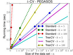
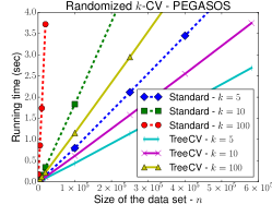
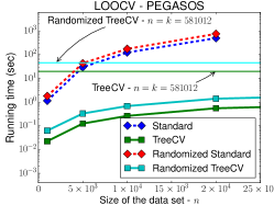
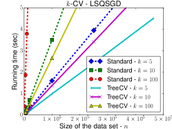
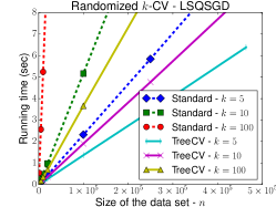
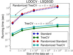
Figure 2 shows the running times of TreeCV and the standard CV method, as a function of $n$, for PEGASOS (top row) and LSQSGD (bottom row). The first two columns show the running times for different values of $k$, with and without randomizing the order of the data points (middle and left column, resp.), while the rightmost column shows the the running time (log-scale) for LOOCV calculations. TreeCV outperforms the standard method in all of the cases. It is notable that TreeCV makes the calculation of LOOCV practical even for $n=581{,}012$, in a fraction of the time required by the standard method at $n=10{,}000$: for example, for PEGASOS, TreeCV takes around $20$ seconds ($46$ when randomized) for computing LOOCV at $n=581{,}012$, while the standard method takes around $124$ seconds ($175$ when randomized) at $n=10{,}000$. Furthermore, one can see that the variance reduction achieved by randomizing the data points comes at the price of a constant factor bigger running time (the factor is around $1.5$ for the standard method, and $2$ for TreeCV). This comes from the fact that both the training time and the time of generating a random perturbation is linear in the number of points (assuming generating a random number uniformly from $\{1,\ldots,n\}$ can be done in constant time).

6 Conclusion

We presented a general method, TreeCV, to speed up cross-validation for incremental learning algorithms. The method is applicable to a wide range of supervised and unsupervised learning settings. We showed that, under mild conditions on the incremental learning algorithm being used, TreeCV computes an accurate approximation of the $k$-CV estimate, and its running time scales logarithmically in $k$ (the number of CV folds), while the running time of the standard method of training $k$ separate models scales linearly with $k$.

Experiments on classification and regression, using two well-known incremental learning algorithms, PEGASOS and least-square SGD, confirmed the speedup and predicted accuracy. When the model learned by the learning algorithm depends on whether the data is provided incrementally or in batch (or on the order of the data, as in the case of online algorithms), the CV estimate calculated by our method was still close to the CV computed by the standard method, but with a lower variance.

References

- An et al. (2007) S. An, W. Liu, and S. Venkatesh. Fast cross-validation algorithms for least squares support vector machine and kernel ridge regression. Pattern Recognition, 40(8):2154–2162, August 2007.
- Cauwenberghs and Poggio (2001) G. Cauwenberghs and T. Poggio. Incremental and decremental support vector machine learning. Advances in neural information processing systems, pages 409–415, 2001.
- Cawley (2006) G.C. Cawley. Leave-One-Out Cross-Validation Based Model Selection Criteria for Weighted LS-SVMs. In International Joint Conference on Neural Networks, 2006. IJCNN ’06, pages 1661–1668, 2006.
- Cesa-Bianchi et al. (2004) N. Cesa-Bianchi, A. Conconi, and C. Gentile. On the generalization ability of on-line learning algorithms. IEEE Transactions on Information Theory, 50:2050–2057, 2004.
- Chang and Lin (2011) C.-C. Chang and C.-J. Lin. LIBSVM: A library for support vector machines. ACM Transactions on Intelligent Systems and Technology, 2:27:1–27:27, 2011. Datasets available at http://www.csie.ntu.edu.tw/~cjlin/libsvmtools/datasets/.
- Christmann and Messem (2008) A. Christmann and A. van Messem. Bouligand derivatives and robustness of support vector machines for regression. The Journal of Machine Learning Research, 9:915–936, 2008.
- Clarkson et al. (2012) K. L. Clarkson, E. Hazan, and D. P. Woodruff. Sublinear optimization for machine learning. Journal of the ACM, 59(5):23:1–23:49, November 2012.
- Debruyne et al. (2008) M. Debruyne, M. Hubert, and J. A. K. Suykens. Model selection in kernel based regression using the influence function. Journal of Machine Learning Research, 9(10), 2008.
- Girard (1989) A. Girard. A fast ‘Monte-Carlo cross-validation’ procedure for large least squares problems with noisy data. Numerische Mathematik, 56(1):1–23, January 1989.
- Golub and von Matt (1997) G. H. Golub and U. von Matt. Generalized Cross-Validation for Large-Scale Problems. Journal of Computational and Graphical Statistics, 6(1):1–34, March 1997.
- Golub et al. (1979) G. H. Golub, M. Heath, and G. Wahba. Generalized Cross-Validation as a Method for Choosing a Good Ridge Parameter. Technometrics, 21(2):215–223, May 1979.
- Görnitz et al. (2013) N. Görnitz, M. Kloft, K. Rieck, and U. Brefeld. Toward supervised anomaly detection. Journal of Artificial Intelligence Research, 46(1):235–262, 2013.
- Izbicki (2013) M. Izbicki. Algebraic classifiers: a generic approach to fast cross-validation, online training, and parallel training. In Proceedings of the 30th International Conference on Machine Learning (ICML 2013), pages 648–656, May 2013.
- Kakade and Tewari (2009) S. M. Kakade and A. Tewari. On the generalization ability of online strongly convex programming algorithms. In Advances in Neural Information Processing Systems, pages 801–808, 2009.
- Lichman (2013) M. Lichman. UCI machine learning repository, 2013.
- Liu et al. (2014) Y. Liu, S. Jiang, and S. Liao. Efficient Approximation of Cross-Validation for Kernel Methods using Bouligand Influence Function. In Proceedings of the 31st International Conference on Machine Learning (ICML 2014), volume 32 of JMLR W&CP, pages 324–332, 2014.
- Mullin and Sukthankar (2000) M. D. Mullin and R. Sukthankar. Complete Cross-Validation for Nearest Neighbor Classifiers. In Proceedings of the 17th International Conference on Machine Learning (ICML 2000), pages 639–646, 2000.
- Nemirovski et al. (2009) A. Nemirovski, A. Juditsky, G. Lan, and A. Shapiro. Robust stochastic approximation approach to stochastic programming. SIAM Journal on Optimization, 19(4):1574–1609, 2009.
- Nguyen et al. (2001) N. Nguyen, P. Milanfar, and G. Golub. Efficient generalized cross-validation with applications to parametric image restoration and resolution enhancement. IEEE Transactions on Image Processing, 10(9):1299–1308, September 2001.
- Pahikkala et al. (2006) T. Pahikkala, J. Boberg, and T. Salakoski. Fast n-fold cross-validation for regularized least-squares. In In: Proceedings of the Ninth Scandinavian Conference on Artificial Intelligence (SCAI), 2006.
- Shalev-Shwartz et al. (2011) S. Shalev-Shwartz, Y. Singer, N. Srebro, and A. Cotter. Pegasos: Primal estimated sub-gradient solver for svm. Mathematical Programming, 127(1):3–30, 2011.
- Wahba (1990) G. Wahba. Spline models for observational data, volume 59. SIAM, 1990.