Evidence for a [WR] or WEL–type binary nucleus in the bipolar planetary nebula Vy 1–2

Abstract

We present high–dispersion spectroscopic data of the compact planetary nebula Vy 1–2, where high expansion velocities up to 100  km s^-1 are found in the H$\alpha$, [N ii] and [O iii] emission lines. HST images reveal a bipolar structure. Vy 1–2 displays a bright ring–like structure with a size of 2.4″$\times$3.2″ and two faint bipolar lobes in the west–east direction. A faint pair of knots is also found, located almost symmetrically on opposite sides of the nebula at PA=305^∘. Furthermore, deep low–dispersion spectra are also presented and several emission lines are detected for the first time in this nebula, such as the doublet [Cl iii] 5517, 5537 Å, [K iv] 6101 Å, C ii 6461 Å, the doublet C iv 5801, 5812 Å. By comparison with the solar abundances, we find enhanced N, depleted C and solar O. The central star must have experienced the hot bottom burning (CN–cycle) during the $\rm{2^{nd}}$ dredge–up phase, implying a progenitor star of M$\geq$3 M_⊙. The very low C/O and N/O abundance ratios suggest a likely post–common envelope close binary system.

A simple spherically symmetric geometry with either a blackbody or a H–deficient stellar atmosphere model is not able to reproduce the ionisation structure of Vy 1–2. The effective temperature and luminosity of its central star indicate a young nebula located at a distance of $\sim$9.7 kpc with an age of $\sim$3500 years. The detection of stellar emission lines, C ii 6461 Å, the doublet C iv$\lambda\lambda$ 5801, 5812 and O iii 5592 Å, emitted from a H–deficient star, indicates the presence of a late–type Wolf–Rayet or a WEL type central star.

1 Introduction

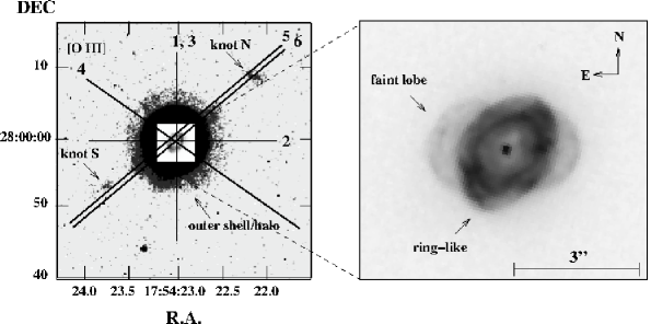
Figure 1: Slit positions of the low–(1) and high–(2, 3, 4 and 5) dispersion spectra superimposed upon the high–resolution HST WFPC3 narrow–band [O iii] image (ID: 11657; PI: Stanghellini). Left panel reveals the presence of a pair of knots at P.A.=305^∘. Right panel is in logarithmic scale and illustrates the ellipsoidal structure of the nebula with extended filamentary structures and the presence of two fainter lobes at P.A. $\sim$90^∘.

Planetary nebulae (PNe) are the consequent result of the interaction of stellar winds ejected from low–to–intermediate mass stars (1-8 M_⊙). A slow and dense wind ($10^{-4}$ M_⊙), emerges from an Asymptotic Giant Branch (AGB) star, is swept up into a dense spherically symmetric shell by a second, faster and tenuous wind expelled during the post-AGB phase (interacting stellar wind model; Kwok et al. 1978). This model can reasonably explain the formation and evolution of spherical PNe. However, most post–AGB stars and PNe show highly asymmetric circumstellar envelopes and complex morphologies (Manchado et al. 2006, Meixner et al. 1999, Parker et al. 2006, Boumis et al. 2003, 2006, Miszalski et al. 2008, Lagadec et al. 2011, Sahai 2011, Sabin et al. 2014).

The deviation of PNe from spherically symmetric structures has its origin in an enhanced equatorial–to–polar density gradient in the AGB circumstellar envelopes resulting in the formation of aspherical and more complex nebulae. This equatorial density enhancement is interpreted as the result of common envelope evolution of close binary systems (Soker & Livio 1994, Nordhaus & Blackman 2006, De Marco 2009). Although, most of the post–AGB and PNe show complex morphologies, only a small number of them are known to contain a binary system (Miszalski et al. 2009, De Marco 2009). Recent work by Jones et al. (2014) confirmed the binary nature of Hen 2–11’s nucleus, providing further evidence of a positive link between binary nuclei and aspherical PNe.

The compact planetary nebula Vy 1–2 (PNG 053.3+24.0), discovered by Vyssotsky (1942), had first been described as an elliptical PN ($``$The IAC Morphological Catalogue of Northern Galactic Planetary Nebulae”; Manchado et al. 1996), but recent high angular resolution HST images revealed a more complex structure (Sahai et al. 2011, Shaw et al. in preparation). According to Winberger’s catalogue of expansion velocities of Galactic PNe, Vy 1–2 shows $\rm{V_{[O{\sc\ III}]}}$ $>$ $\rm{V_{[N{\sc\ II}]}}$ (Weinberger 1989). This result is inconsistent with a simple homologous expansion law. A similar velocity trend has also been found for few other PNe, (e.g. BD +30^∘3639, Akras & Steffen 2012, Bryce & Mellema 1999; see also Medina et al. 2006 for more objects). A detailed study of the velocity field as a function of distance from the central stars in PNe has revealed a more complex expansion law than the simple homologous–law, probably associated with the fast wind from the central stars (Gesicki & Zijlstra 2003). Interestingly, the central stars of this rare group of PNe have been identified as Wolf–Rayet type ([WR]) or weak emission line stars (WELS) (Medina et al. 2006). Unfortunately, the spectral type of the central star of Vy 1–2 is still unknown. Barker (1978a,b), and more recently Wesson et al. (2005), as well as Stanghellini et al. (2006) studied the ionisation structure and chemical composition of this nebula. A comparison between these studies shows a significant discrepancy in the ionic and total chemical abundances (see Tables 5 and 6). This may be related to the different values of T_e and N_e used by these authors. In particular, Wesson et al. (2005) estimated N_e and T_e using diagnostics line ratios from low to high excitation lines (see Table 4). The high difference in N_e between [S ii] and [O ii] cannot be explained since they have similar ionisation potentials. Barker (1978a) gave an average value of 5000 cm^-3 using different diagnostics from low excitation lines ([S ii] and [O ii]). Therefore, the low $\rm{N_{e}}$ in [S ii] of 1160 cm^-3 derived by Wesson et al. (2005), may not be correct.

Table 1: Observation log

Slit	Dispersion	Date	Filter	wavelength (Å)	FWHM (Å)	P.A. (∘)	Exp. times (sec)
				1.3m Skinakas Telescope
1	low	2011 Sep 04	$-$	4700–6800	$-$	0	3600 and 300$\times$3
				2.1m SPM Telescope $+$ MES
2	high	2011 May 15	H$\alpha$+[N ii]	6550	90	90	1800
2	high	2011 May 15	[O iii]	5007	60	90	1800
3	high	2012 Mar 30	H$\alpha$+[N ii]	6550	90	0	1200
4	high	2012 Apr 01	H$\alpha$+[N ii]	6550	90	55	1200
5	high	2012 Apr 01	H$\alpha$+[N ii]	6550	90	310	1800
5	high	2012 Apr 01	[O iii]	5007	60	310	1800
6a	high	2002 Jul 23	H$\alpha$+[N ii]	6550	90	310	1800
				HST+WFPC3
$-$	imaging	2010 Feb 08	F502N	5010.0	65.0	$-$	600
$-$	imaging	2010 Feb 08	F200LP	4883.0	5702.2	$-$	11
$-$	imaging	2010 Feb 08	F350LP	5846.0	4758.0	$-$	11
$-$	imaging	2010 Feb 08	F814W	8024.0	1536.0	$-$	23

^a It was drawn from the SPM Kinematic Catalogue of Planetary Nebulae

The logarithmic H$\beta$ flux (erg s^-1 cm^-2) was estimated to be -11.52$\pm$0.01 (Barker 1978a; hereafter Bar78a) and -11.53 (Wesson et al. 2005; hereafter WLB05). Vy 1–2 is also a radio source with 1.4 GHz flux equal to $12.4\pm 0.9$ mJy and extinction coefficient c(radio)=0.1, which is slightly lower than the optical value from WLB05 (c(H$\beta$)=0.139). The coordinates of Vy 1–2 are given at RA $\rm{17^{h}54^{m}23^{s}}$ and Dec. $\rm{27\degr\ 59\arcmin\ 58\arcsec}$ for the optical, and RA $\rm{17^{h}54^{m}23^{s}.49}$ and Dec. $\rm{+27\degr\ 59\arcmin\ 58\arcsec.5}$ for the radio position (Condon & Kaplan 1998).

The first estimation of the effective temperature of the central star of Vy 1–2 was by Gurzadyan (1988), 124 kK and 66 kK using the He ii/ H$\beta$ and [O iii]/ He ii line ratios, respectively. More recently, Stangellini et al. (2002) calculated $\rm{T_{eff}}$ = 119$\pm 25$ kK and $\rm{log(L/L_{\odot}})$ = 3.275$\pm$0.285, for a distance of $7.24\pm 0.13$ kpc, whereas Phillips (2003) estimated the He i and He ii Zanstra temperatures of $75.4\pm 10.2$ kK and $99.8\pm 4.3$ kK, respectively. Its distance is uncertain. It has been estimated to range from 4.38 kpc to 7.6 kpc: 4.7 kpc (Maciel 1984); 5.7 kpc (Sabbadin et al. 1984); 4.38 kpc (Phillips 1998) and 7.6 kpc (Cahn & Kaler 1971, Cahn et al. 1992). However, all the aforementioned authors used a radius of 2.4″ for their distance estimation obtained from Cahn and Kaler (1971). No high–angular resolution of Vy 1–2 had been obtained until 1996 (Manchado et al. 1996). More recently, Shaw et al. (in preparation) obtained the high–angular HST images that we present here. The value of 2.4″ is almost $\sim$1.6 times larger than the radius find in this work using the HST images (see below). This implies that the previous reported distances of Vy 1–2 are likely underestimated.

The large differences in chemical abundances and effective temperature inspired us to study this nebula and provide more accurate determinations of stellar and nebular properties. We present high–resolution HST images of Vy 1–2 in the [O iii] emission line and broad–band filter F200LP, as well as new high– and low–dispersion spectra in order to provide further insight into the kinematic structure and chemical composition of this compact nebula. In Section 2, we describe the observations and data reduction procedures. In Section 3, we present the results from the morpho–kinematic and chemical analysis. We also present the physical properties and chemical abundances derived from the ionisation correction factor (ICF; Kingsburgh & Barlow 1994) and from a photo–ionisation model performed with Cloudy (Ferland et al. 2013). Our results are discussed in Section 4 and conclusions are summed up in Section 5.

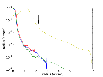
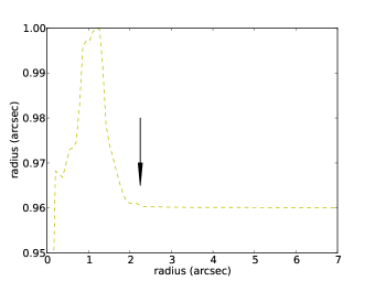
Figure 2: Left panel: surface brightness profile of [O iii] emission in Vy 1–2 averaged over all angles (yellow dashed line). The bump at r$\sim$2.2 ″–2.3 ″, indicated by an arrow, corresponds to the contribution of the faint lobes along the east–west direction. The red and blue solid lines represent the radial brightness of two stars observed with the same camera and filter while the green solid line corresponds to the profile of a theoretical HST point spread function (PSF) created using the program Tiny Tim. Right panel: surface brightness profile of the convolved [O iii] image averaged over all angles, using the theoretical PSF and Leon Lucy’s algorithm.

2 Observations

2.1 HST imaging

High–resolution HST images of Vy 1–2 were drawn from the Mikulski archive for space telescopes (Shaw et al. in preparation). They were taken with the Wide Field Planetary Camera 3 (WFPC3) on February 8^th 2010 (GO program 11657, PI: Stanghellini L.). The narrow–band F502N filter ($\lambda$=5009.8 Å) was used to isolate the [O iii] 5007 Å emission line and determine the morphology of Vy 1–2 (Fig. 1), while the broad filters F200LP, F350LP and F814W ($``$I”, see Table 1) were obtained in order to probe the presence of a cold binary companion. The exposure times were 600, 11, 11, and 23 sec, respectively. A faint outer shell or halo as well as a pair of knots can be discerned in the [O iii] image (Fig. 1, left panel), while the F200LP (Fig 1, right panel) image is used to highlight the inner nebular components: the bright elliptical ring–like structure and the faint lobes.

We carefully investigate whether the outer shell/halo is a real nebular component or the result of scattered light from the bright inner nebula in the HST optics. In Figure 2, left panel, we display the radial profile of a theoretical PSF (green solid line), of two field stars (observed with the same camera and filter; red and blue solid lines) and of Vy 1–2 (yellow dashed line). The radial profiles between the two field stars and the theoretical PSF agree reasonably well. A discrepancy with the modelled PSFs can be seen at around 1.5–2″, though it is negligible compared to the Vy 1–2’s profile. On the other hand, Vy 1–2 shows a maximum brightness at r=1.2″ (at the position of the ring–like structure), while for r$>$2.2–2.3″ (indicated by a vertical arrow in Fig. 2) shows a similar steep decline for the stars and theoretical PSF but two magnitude brighter. The theoretical [O iii] PSF was used to convolve the HST image using Leon Lucy’s algorithm in STSDAS. The azimuthally–averaged profile of the convolved image is presented in Figure 2, right panel. The bump at r=2.2–2.3″ is indicated by a vertical arrow. For r$>$2.3″, the profile is a constant function, which means that the outer shell/halo is seen due to the PSF scattering. In particular, for a power-law density distribution of $\rho$(r)$\propto$r^-1, a r^-2 surface brightness is expected (Sahai et al. 1999), which we do not see here. Nevertheless, some contribution of scattering light from dust can not be excluded, given that Vy 1–2 has been found to be a strong IR emitter.

2.2 High–dispersion longslit spectroscopy

High–dispersion, long–slit spectroscopic data of Vy 1–2 in H$\alpha$+[N ii] and [O iii] were obtained using the Manchester echelle spectrometer, (MES–SPM; Meaburn et al. 2003) on the 2.1 m telescope at the Observatorio Astronómico of San Pedro Martir in Baja California, Mexico, in its f/7.5 configuration. The observing run took place on May 2011 and April 2012 (see Table 1). The MES-SPM was equipped with a Marconi CCD detector with 2048$\times$2048 square pixels and each side of 13.5 $\mu$m ($\equiv$0.176″ pixel^-1). A 90 Å bandwidth filter was used to isolate the 87^th order containing the H$\alpha$ and [N ii] $\lambda\lambda~{}$6548, 6584 Å, and the 113^th order containing the [O iii] 5007 Å emission lines. Two-by-two binning was employed in both the spatial and spectral directions (a three–by–three binning was employed in both directions for the observing run in May). Consequently, 1024 increments, each 0$\aas@@fstack{\prime\prime}$352 long, gave a projected slit length of 5$\aas@@fstack{\prime}$12 on the sky. The slit used was 150 $\mu$m wide ($\equiv$ 11  km s^-1 and 1$\aas@@fstack{\prime\prime}$9). During the observations the slit was oriented at different position angles. The integration times were 1800 sec, 1500 sec and 1200 sec (see Table 1 for details). In order to avoid any contamination from the bright central star, the slits were slightly offset from it by $\sim$0.5 ″, covering only the bright ring–like structure.

A faint continuum could be discerned within the very short spectral range of our single–order echelle spectra. The wavelength calibration was performed using a Th/Ar calibration lamp to an accuracy of $\pm$1  km s^-1 when converted to radial velocity. The data reduction was performed using the standard IRAF  and STARLINK routines. Individual images were bias subtracted and cosmic rays removed. All spectra were also calibrated to heliocentric velocity. The position–velocity (PV) diagrams and line profiles for the H$\alpha$, [N ii] and [O iii], and for all slit positions are presented in Figures 4–8 and Figures 9–12, respectively.

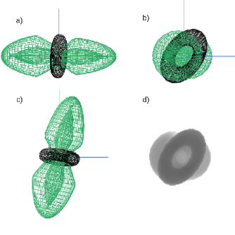
Figure 3: Schematic diagrams of Vy 1–2 using the code SHAPE. Panels a) to c) show the mesh SHAPE images for three different orientations right, front and top views, respectively. Panel d) illustrates the final rendered 2–D image.

2.3 Low–dispersion spectroscopy

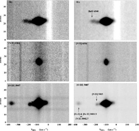
Figure 4: H$\alpha$ (upper panel), [N ii] 6584 Å (middle panel) and [O iii] 5007 Å (lower panel) position–velocity (PV) diagrams of Vy 1–2 shown at two different contrast levels the for slit position 2 (P.A.=90^∘).

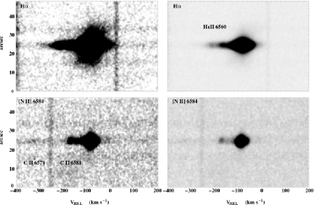
Figure 5: H$\alpha$ (upper panel) and [N ii] 6584 Å (lower panel) position–velocity (PV) diagrams of Vy 1–2 shown at two different contrast levels for the slit position 3 (P.A.=0^∘).

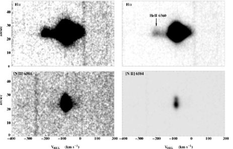
Figure 6: H$\alpha$ (upper panel) and [N ii] 6584 Å (lower panel) position–velocity (PV) diagrams of Vy 1–2 shown at two different contrast levels the for slit position 4 (P.A.=55^∘).

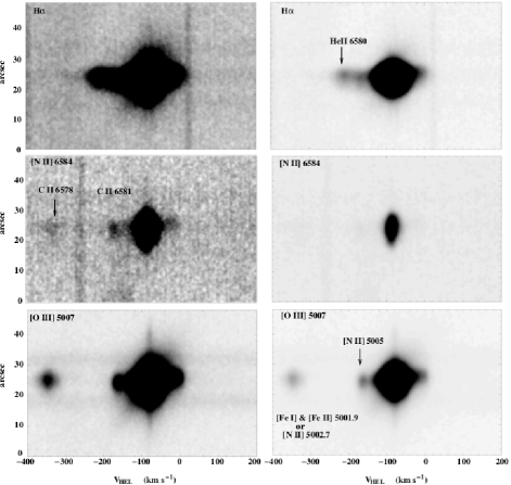
Figure 7: H$\alpha$ (upper panel), [N ii] 6584 Å (middle panel) and [O iii] 5007 (lower panel) position–velocity (PV) diagrams of Vy 1–2 shown at two different contrast levels for the slit position 5 (P.A.=310^∘).

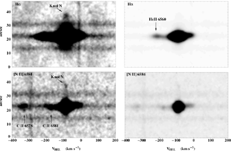
Figure 8: H$\alpha$ (upper panel) and [N ii] 6584 Å (lower panel) position–velocity (PV) diagrams of Vy 1–2 shown at two different contrast levels for the slit position 6 (P.A.=310^∘), drawn from the SPM catalogue (López et al. 2012).

Low–dispersion spectra of Vy 1–2 were obtained with the 1.3 m telescope at Skinakas Observatory in Crete, Greece, on September $\rm{4^{th}}$, 2011. A 1300 line mm^-1 grating was used in conjunction with a 2000 x 800 SITe CCD (15 $\mu$m pixel), resulting in a scale of 1 Å $\rm{pixel^{-1}}$ and covering the wavelength range of 4700–6800 Å. The slit width used was 7.7″ with a slit length of 7.9 ′ and oriented in the north–south direction (Slit position 1). Two different exposure times were taken in order to identify both the bright and faint emission lines: 3600 sec (saturated in H$\alpha$ and [O iii] 5007 Å lines, but detecting the much fainter lines) and 3 x 300 sec. The spectro–photometric standard stars HR5501, HR7596, HR9087, HR718 and HR7950 (Hamuy et al. 1992) were observed in order to flux calibrate the spectra, while the fluxes were also corrected for atmospheric extinction and interstellar reddening.

The data reduction was performed using standard IRAF routines. Individual images were bias subtracted and flat–field corrected using a series of twilight flat–frames. The sky–background was also subtracted from each individual frame while no dark frames were used as the dark current was negligible. Finally, the wavelength calibration was performed using a Fe–He–Ne–Ar calibration lamp.

3 Results

3.1 Morphology

Figure 1 displays the high–resolution HST [O iii] (left panel) and ultraviolet (F200LP, right panel) images of Vy 1–2, at two different scales, in order to highlight the fainter nebular components. The left panel displays a faint outer shell/halo and two much fainter knots at a position angle (hereafter P.A.) of 305^∘, located at 11.5″ (knot S) and 14.5″ (knot N) from the central star. The right panel shows an enlargement of the nebula, revealing a bright elliptical ring–like structure with a minor and major axis of 2.4″ and 3.2″, respectively. This implies a mean radius of $\sim$1.4″. This value is $\sim$1.6 times lower than the value used previously for the distance estimation obtained from ground–based observations. Thus, we recalculated the distance of Vy 1–2 using our more accurate value of radius, and we obtain a distance between 7.0 kpc and 14.5 kpc. These distances clearly indicate that Vy 1–2 is a distant nebula. An average distance of 9.7 kpc is adopted here.

The ring–like structure has a non–uniform emission along its perimeter, with an apparent filamentary structure, which indicates a strong interaction of stellar winds in addition of an inner cavity. Its major axis is oriented towards to a P.A.$=$320^∘, 15^∘ rotated from the knots’ direction. This may be associated with a possible precession of the rotation axis of a single central star, or the orbital plane of a binary star at the centre of Vy 1–2. Two faint lobes are also apparent in the east–west direction (P.A. $\sim$90^∘). Despite their very low surface brightness compared to the central ring-like structure, their morphology suggests a bipolar structure, like the Homunculus nebula and Hb 5 PN. The eastern and western bipolar lobes are found to be blue– and red–shifted, respectively, while their different sizes imply a tilted nebula towards the line of sight. In Figure 3, we illustrate a schematic 3–D diagram of Vy 1–2 for different points of view, using the code SHAPE (Steffen et al. 2011). This simple model reproduces fairly well the main components of Vy 1–2, such as the ring—like structure and the bipolar lobes as well as the orientation of the nebula (inclination and position angles). The inclination angle of the model is 13^∘, while the ring–like structure is best described with an ellipse. Any attempt to reproduce the ring–like structure assuming a round shape, resulted in a very high inclination angle of $\sim$50^∘ that we do not get from the PV diagrams. Our 3-D structure of Vy 1–2 is only one of many other solutions that can be obtained just by varying the size of bipolar lobes and the orientation accordingly.

Moreover, in order to investigate the possible presence of a cold binary companion, the F200LP, F350LP and F814W broad–band images were studied. With the available data, we found no evidence of a nearby companion. If the central star is a binary system, then the projected separation must be smaller than 0.08″.

Table 2: Expansion velocities of Vy 1–2

slit	P.A.	V(H$\alpha$)	V([N ii])	V([O iii])	V(He ii)
	(∘)	km s-1	km s-1	km s-1	km s-1
low velocity component
2	90	19	9	18	25
3	0	18	8	$-$	$-$
4	55	19	9	$-$	25
5	310	19	9	18	23
6	310	19	8	$-$	23
high velocity component
2	90	90	40	90	$-$
3	0	100	40	$-$	$-$
4	55	100	40	$-$	$-$
5	310	95	90	90	$-$
6	310	100	90	$-$	$-$

3.2 Kinematics

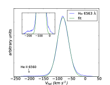
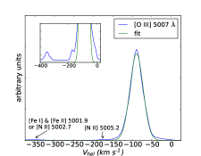
Figure 9: The H$\alpha$, [N ii] 6584 Å and [O iii] 5007 Å line profiles for slit position 2 (P.A.=90^∘) are shown in the left, middle and right panels, respectively. The blue and green lines correspond to the observed line profile and a single Gaussian best fit, respectively.

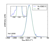
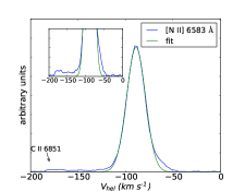
Figure 10: The H$\alpha$ and [N ii] 6584 Å line profiles for slit position 3 (P.A.=0^∘) are shown in the left and right panels, respectively. The blue and green lines correspond to the observed line profile and the single Gaussian best fit, respectively.

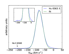
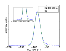
Figure 11: The H$\alpha$ and [N ii] 6584 Å line profiles for slit position 4 (P.A.=55^∘) are shown in the left and right panels, respectively. The blue and green lines correspond to the observed line profile and the single Gaussian best fit, respectively.

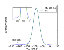
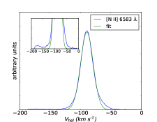
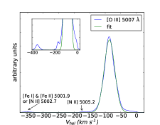
Figure 12: The H$\alpha$, [N ii] 6584 Å and [O iii] 5007 Å line profiles for slit position 5 (P.A.=310^∘) are shown in the left, middle and right panels, respectively. The blue and green lines correspond to the observed line profile and the single Gaussian best fit, respectively.

In Figures 4 to 8 we present the observed H$\alpha$ 6563 Å, [N ii] 6584 Å and [O iii] 5007 Å position–velocity (PV) diagrams along the slit positions 2 to 6. All slit positions are shown overlaid on the HST [O iii] image (Fig. 1, left panel). Besides the common bright H$\alpha$, [N ii] and [O iii] emission lines, the He ii 6560 Å and He i 5015 Å lines, as well as the much weaker lines, C ii 6581.2 Å, C ii 6578 Å, [N ii] 4996.8 Å, [Fe i] + [Fe ii] 5001.9 Å or [N ii] 5002.7 Å, [N ii] 5005.2 Å and [Fe ii] 5018.2 or He i 5017.2 Å are also present (see Figs 4 to 8).

By conducting a literature search for these emission lines in well known objects, we found a small number of PNe (e.g NGC 6543, Hyung et al. 2000; M 2–9, Lee H.–W. et al. 2001) and symbiotic stars (RR Telescopii and He 2–106, Lee H.–W. et al. 2001) that exhibit the 6581 Å emission line. However, those objects also exhibit the 6545 Å line, which usually is attributed to the Raman scattered He ii line that is not detected in our data. Both the 6578 Å and 6581 Å lines have also been detected in the symbiotic star AE Circinus, and identified as carbon lines (Mennickent et al. 2008). The 5002 Å line has been detected in the J320 (PNG190.3−17.7) nebula but no identification was provided (Harman et al. 2004).

The PV diagrams clearly show the presence of a high–speed component (wide wings) with velocities up to 90–100  km s^-1, and a much slower component $\sim$20  km s^-1 (Gaussian fit). The H$\alpha$ 6563 Å, [N ii] 6584 Å and [O iii] 5007 Å emission line profiles, in Fig. 9 to 12, are from the slit positions 2 to 5, respectively. Single Gaussian fit to these line profiles gives turbulent widths (FWHM) of 19$\pm$3  km s^-1 in the H$\alpha$, between (8–9)$\pm$2  km s^-1 in the [N ii], and $18\pm$3  km s^-1 in the [O iii] emission (see Table 2). These expansion velocities correspond to the bright, inner ring–like structure. Two separated blobs can be discerned in the [N ii] 6584 Å PV diagram from the slit position 4 (Fig. 6; right, lower panel), similar to those of a pole–on toroidal or ring–like structure, whilst high expansion velocities are not apparent, since this slit position covers only a small part of the bipolar lobes. All the widths are corrected: for the 20  km s^-1 instrumental width; the 21.4  km s^-1 thermal width of the H$\alpha$ line at 10000 K (5.8  km s^-1and 5.4  km s^-1of the [N ii] and [O iii] lines respectively); and the fine structural broadening of 6.4  km s^-1 of the H$\alpha$ line. Note that, unlike the H$\alpha$ line, the [N ii] and [O iii] lines have no fine structural components. The He ii expansion velocity is estimated (23–25)$\pm$4  km s^-1 from the He ii 6560 Å recombination line, and is corrected for the instrumental broadening of 20  km s^-1, the thermal broadening of 10.7  km s^-1 (10000 K), and the fine structural broadening from this line at $\sim$6  km s^-1 (Meaburn et al. 2005).

Additional to the previous low velocity components, the line profiles of Vy 1–2 also present broad wings (Figs. 9–12). This continuous high–velocity component likely corresponds to the expansion of the faint bipolar lobes seen in the HST images. $\rm{V_{[O{\sc\ III}]}}$ is between 90$\pm$4  km s^-1and 100$\pm$4  km s^-1, measured at the base of line profiles for all the P.A. The [N ii] emission line shows such high expansion velocity of 90–100  km s^-1 only along the P.A.=310^∘, whilst for the rest of the P.A.s, $\rm{V_{[N{\sc\ II}]}}$ is significantly lower than $\rm{V_{[O{\sc\ III}]}}$. This is in agreement with the Winberger’s catalogue (Weinberger 1989). A similar velocity trend, $\rm{V_{[O{\sc\ III}]}}$ $>$ $\rm{V_{[N{\sc\ II}]}}$, has also been reported for a small group of PNe (see §4.1). Regarding the HST images and PV diagrams, we conclude that Vy 1-2 is seen almost pole–on with an inclination angle of 10^∘ $\pm$2^∘ to the line of sight. The average systemic velocity of the nebula is $V_{\rm{sys}}$=-85  km s^-1, with a standard deviation of 4  km s^-1, in good agreement with the previous value of -82.4$\pm$3.9 km s^-1 quoted by Schneider et al. (1983).

Figure 8 shows the PV diagram obtained along P.A.=305^∘ in H$\alpha$+[N ii], drawn from the recently released SPM Kinematic Catalogue of Galactic Planetary Nebulae (López et al. 2012). This spectrum covers, apart from the bright ring–like structure, the faint knot N (Fig. 1). The H$\alpha$ line profile of this knot is centred on $V_{\rm{HEL}}$=-80$\pm$4  km s^-1. This central value should be compared to the systemic heliocentric radial velocity of the whole nebula, $V_{\rm{sys}}$=-85$\pm$4  km s^-1.

Table 3: Observed and modelled emission line intensities for Vy 1–2, corrected for interstellar extinction. The lines outside the wavelength range 4700–6800 Å were drawn from WLB05.

Line(Å)	I($\lambda$)	error	model	WLB05
[O ii] 3726	$-$	$-$	17.69	20.04
[O ii] 3729	$-$	$-$	9.57	9.97
[Ne iii] 3869	$-$	$-$	98.86	94.55
[Ne iii] 3968	$-$	$-$	29.81	29.91
He i 4026	$-$	$-$	2.05	2.19
[S ii] 4070	$-$	$-$	1.49	1.21
H$\gamma$ 4100	$-$	$-$	25.89	24.44
H$\delta$ 4340	$-$	$-$	46.81	45.30
[O iii] 4363	$-$	$-$	9.12	8.51
He i 4471	$-$	$-$	4.39	4.40
He ii 4686	$-$	$-$	26.85	31.00
He i 4712	$-$	$-$	0.54	0.52
[Ar iv] 4712	3.89	0.43	3.38	4.29
[Ar iv] 4740	3.97	0.48	3.72	4.22
H$\beta$ 4861	100.00	4	100.00	100.0
He i 4924	1.38	0.34	1.18	1.15
[O iii] 4959	434.85	13	497.21	443.10
[N ii] 4997b	$-$	$-$	$-$	$-$
[Fe ii] 5002b	$-$	$-$	$-$	$-$
[N ii] 5003b	$-$	$-$	$-$	$-$
[N ii] 5005b	$-$	$-$	$-$	$-$
[O iii] 5007	1287.06	38	1496.59	1337.0
He i 5015b	$-$	$-$	$-$	$-$
He i 5017b	$-$	$-$	$-$	$-$
[Fe ii] 5018b	$-$	$-$	$-$	$-$
[Si ii] 5040a	0.25	0.09	$-$	$-$
[N i] 5200	0.22	0.07	0.00	$-$
He ii 5411	2.15	0.19	1.95	$-$
[Cl iii] 5517	0.56	0.11	0.52	$-$
[Cl iii] 5537	0.64	0.16	0.61	$-$
[O i] 5577a	0.05	0.03	0.001	$-$
[N ii] 5678	0.13	0.04	0.00	$-$
[N ii] 5755	0.53	0.11	0.42	$-$
He i 5876	13.16	0.71	13.11	13.10
[K iv] 6101a	0.23	0.06	$-$	$-$
He ii 6119	0.11	0.04	0.06	$-$
He ii 6172	0.08	0.04	0.06	$-$
He ii 6234	0.08	0.04	0.07	$-$
[O i] 6300	2.02	0.14	0.06	1.70
[S iii] 6312	1.45	0.15	5.09	1.30
[O i] 6363	0.69	0.09	0.02	0.71
He ii 6405	0.11	0.04	0.11	$-$
[Ar v] 6435	0.17	0.06	0.43	$-$
He ii 6525	0.17	0.06	0.13	0.5
[N ii] 6548	8.42	0.45	8.75	9.16
He ii 6560b	$-$	$-$	$-$	$-$
H$\alpha$ 6563	284.62	10	287.45	284.1
C ii 6578b	$-$	$-$	$-$	$-$
C ii 6581b	$-$	$-$	$-$	$-$
[N ii] 6584	26.23	1.32	25.81	22.68
He i 6678	3.79	0.31	3.59	3.89
[S ii] 6716	2.49	0.28	2.61	2.04
[S ii] 6731	4.13	0.32	4.69	2.47
[Ar v] 7005	$-$	$-$	0.95	0.61
He i 7065	$-$	$-$	4.39	3.96
[Ar iii] 7135	$-$	$-$	12.51	13.83
He i 7281	$-$	$-$	0.70	0.50
[Ar iii] 7751	$-$	$-$	3.01	2.61
logF(H$\beta$)	-11.56	—-	-11.56	-11.53

Table 3: Continued

Line(Å)	I($\lambda$)	error	model	WLB05
[O iii] 5007/4363	$-$	$-$	164	157
[N ii] 6581/5755	49.5	10.4	61.4	$-$
[O i] 6300+6363/5577	54.2	28.1	80.0	$-$
[O ii] 3727/3729	$-$	$-$	1.85	2.01
[S ii] 6716/6731	0.60	0.12	0.56	0.83
[Ar iv] 4712/4740	0.98	0.27	0.92	1.01
[Cl iii] 5517/5537	0.88	0.36	0.85	$-$
J  1.25c	3.5d	0.2d	2.4	$-$
H  1.65	2.0	0.1	2.3	$-$
K  2.15	2.6	0.1	2.8	$-$
WISE  3.35	3.4	0.1	2.5	$-$
WISE  4.60	5.6	0.1	2.2	$-$
AKARI  9.00	104	21	65	$-$
WISE  11.6	164.	21	110	$-$
IRAS  12.0	113	22	211	$-$
AKARI  18.0	786	21	893	$-$
WISE  22.1	1319	15	1804	$-$
IRAS  25.0	1647	83	2361	$-$
IRAS  60.0	2078	104	2122	$-$
AKARI  65.0	1704	$-^{e}$	1795	$-$
AKARI  90.0	1184	58	796	$-$
IRAS  100.0	1094	219	592	$-$
AKARI  140.0	697	$-^{e}$	218	$-$

^a These lines were not used to constrain the model.

^b Emission lines detected in the high–dispersion spectra

^c In $\mu$m, ^d In mJy

^e No errors are provided for these measurements since the flux quality indicator is 1.

3.3 Ionisation structure

3.3.1 Nebular parameters and ICF abundances

The panels in Figure 13 display the low–dispersion spectra of Vy 1–2 that cover the wavelength range of 4700–6800 Å for exposure times of 3600 (upper panel) and 300 sec (lower panels), respectively. Several emission lines from low–to–high and very high ionisation states are present and some are detected for the first time in this nebula. Besides the common nebular lines, such as H$\alpha$, H$\beta$, He i, He ii, [O iii], [N ii] and [S ii] lines, the [Cl iii] 5517 and 5537 Å, C ii 6461 Å, C iv 5801 and 5812 Å, [Si ii] 5040 Å, [K iv] 6101 Å and [N ii] 5679 Å emission lines are also detected.

It is worth mentioning here that the emission line at 5679 Å has been identified either as the [N ii] line by Liu et al. (2000; NGC 6135, 2001; M1–42 and M2–36) and Ercolano et al. (2004; NGC 1501), or as [Fe vi] line by Hyung & Aller (1997). However, the latter classification requires, a very hot star of $\rm{T_{eff}}\geq$140 kK, which is not in agreement with the values previously published ($\rm{T_{eff}}$=119 kK, Stangellini et al. 2002; 75.4 kK$<\rm{T_{eff}}<$99 kK, Phillips 2003).

All very faint emission lines presented here are only detected in our deep spectrum ($\rm{t_{exp}}$=3600 sec). Notice that WLB05 did not detect any of these lines due to their shallow spectroscopy.

In Table 3, we list the optical nebular emission line fluxes, corrected for atmospheric extinction and interstellar reddening. All line fluxes are normalized to F(H$\beta$)=100. The interstellar extinction c(H$\beta$) was derived from the Balmer H$\alpha$/H$\beta$ ratio (Eq. 1), using the interstellar extinction law by Fitzpatrick (1999) and $R_{v}$=3.1,

$$c(H\beta)=\frac{1}{0.348}log\frac{F(H\alpha)/F(H\beta)}{2.85},$$ (1)

where the 0.348 is the relative logarithmic extinction coefficient for H$\beta$/H$\alpha$. The observed reddening in magnitude E(B-V) was also calculated using the following relationship (Seaton 1979),

$$c(H\beta)=0.4X_{\beta}E(B-V),$$ (2)

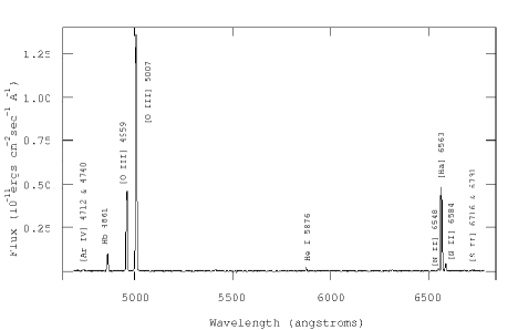
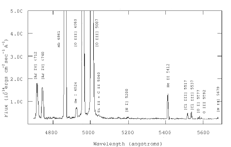
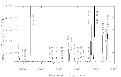
Figure 13: Observed spectra of Vy 1–2 taken with the 1.3–m telescope. Upper panel displays the spectrum with an exposure time of 300s, covering the wavelength range of 4700–6800 Å. Lower panels display two enlargements of the spectrum (left: 4700–5700 Å, right: 5700–6800 Å) with an exposure time of 3600 sec, in order to highlight the weaker emission lines.

where the extinction parameter $\rm{X_{\beta}}$ = 3.615 (Fitzpatrick 1999). The errors of the extinction c(H$\beta$) and E(B-V) are calculated through standard error propagation of equations (1) and (2). We obtain c(H$\beta$)=0.13$\pm$0.03, in agreement with the value quoted by WLB05 (c(H$\beta$)=0.139) and E(B-V)=0.09$\pm$0.02. Our logarithm H$\beta$ flux -11.56$\pm$0.03 is also in very good agreement with previous studies (-11.53, WLB05; -11.52, Bar87a) and the recently published catalogue of integrated H$\alpha$ fluxes of Galactic PNe (Frew et al. 2013). Notice that the interstellar extinction c(H$\beta$) of Vy 1–2, given by Frew et al. (2013) is significantly lower than the previous values.

Table 4: Electron temperature (in K) and electron density (in $\rm{cm^{-3}}$) of Vy 1–2.

	this work	WLB05	Bar78a	McNabb†
$\rm{T_{e}}$([O iii])	$-$	10400	9800	$-$
$\rm{T_{e}}$([N ii])	10850$\pm$2100	$-$	$-$	$-$
$\rm{T_{e}}$([O ii])	$-$	16179	$-$	7943
$\rm{T_{e}}$([O i])	10400$\pm$5400	$-$	$-$	$-$
$\rm{N_{e}}$([S ii])	4500$\pm$650	1160	5000	$-$
$\rm{N_{e}}$([Cl iii])	4330$\pm$1600	$-$	$-$	$-$
$\rm{N_{e}}$([Ar iv])	4550$\pm$1300‡	3300	$-$	$-$
$\rm{N_{e}}$([O ii])	$-$	4100	$-$	4466

${\dagger}$ T_e[O ii] and N_e[O ii] estimated by McNabb et al. are obtained using the O ii optical recombination lines.

${\ddagger}$ The contribution of He i 4712 Å emission line to [Ar iv] 4711 Å line, was calculated based on the work of Benjamin et al. (1999).

Table 5: Ionic and total ( $\epsilon$(X)=log(n(X)/n(H))+12) abundances derived from the observed fluxes of Vy 1–2.

ionic	this work	this work	WLB05	Bar78b
abundances	(ICF)	(model)
$\rm{He^{+}/H^{+}}$	0.087$\pm$0.008	0.083	0.084	0.076
$\rm{He^{++}/H^{+}}$	0.022$\pm$0.004	0.024	0.023	0.019
ICF(He)	1.00	1.00	1.00	1.0
$\rm{\epsilon(He)}$	11.04$\pm$0.03	11.03	11.03	10.98
$10^{5}\times\rm{O^{+}/H^{+}}$	1.55$\pm$0.17a	2.35	1.36	2.51
$10^{5}\times\rm{O^{2+}/H^{+}}$	37.74$\pm$2.78	66.11	41.55	47.1
ICF(O)	1.17	1.19	1.18	1.25
$\rm{\epsilon(O)}$	8.66$\pm$0.04	8.91	8.70	8.79
$10^{5}\times\rm{N^{+}/H^{+}}$	0.47$\pm$0.05	0.62	0.395	0.435
$10^{5}\times\rm{N^{2+}/H^{+}}$	$-$	$-$	9.300	$-$
ICF(N)	29.28	41.45	1.206	24.8
$\rm{\epsilon(N)}$	8.13$\pm$0.05	8.43	8.06	8.03
$10^{6}\times\rm{S^{+}/H^{+}}$	0.24$\pm$0.04	0.38	0.144	0.385
$10^{6}\times\rm{S^{2+}/H^{+}}$	2.71$\pm$0.37	12.19	2.467	$-$
ICF(S)	2.17	1.86	2.334	24.8
$\rm{\epsilon(S)}$	6.80$\pm$0.08	7.37	6.78	6.98
$10^{8}\times\rm{Cl^{2+}/H^{+}}$	7.09$\pm$1.97	10.07	$-$	$-$
ICF(Cl)	2.35	2.03	$-$	$-$
$\rm{\epsilon(Cl)}$	5.22$\pm$0.12	5.31	$-$	$-$
$10^{7}\times\rm{Ar^{2+}/H^{+}}$	11.23$\pm$1.35a	13.03	9.370	$-$
$10^{7}\times\rm{Ar^{3+}/H^{+}}$	6.26$\pm$1.43	10.34	6.902	$-$
$10^{7}\times\rm{Ar^{4+}/H^{+}}$	0.75$\pm$0.26	1.09	1.005	$-$
ICF(Ar)	1.04	1.01	1.035	$-$
$\rm{\epsilon(Ar)}$	6.28$\pm$0.06	6.39	6.25	$-$

^a The ionic abundances of these ions were calculated using the intensities from WLB05, considering an error of 10%, since no errors are given in WLB05.

The nebular electron temperature ($\rm{T_{e}}$) and density ($\rm{N_{e}}$) are derived using the TEMDEN task in IRAF (Shaw & Dufour 1994). From the [N ii] (6584+6548)/5755 and [O i] (6300+6363)/5577 diagnostic line ratios, we obtain $\rm{T_{e}}$= 10850$\pm$2100 K and 10400$\pm$5400 K, respectively, whilst $\rm{N_{e}}$ are calculated as 4500$\pm$650 $\rm{cm^{-3}}$, 4330$\pm$1600 $\rm{cm^{-3}}$ and 4550$\pm$1300 $\rm{cm^{-3}}$ from the [S ii] 6716/6731, [Cl iii] 5517/5537 and [Ar iv] 4711/4740 diagnostic line ratios, respectively. No evidence of density variation with the ionisation potential is found (see also Fig. 14). For direct comparison, Table 4 lists the $\rm{N_{e}}$ and $\rm{T_{e}}$ together with those derived in previous studies from collisionally excited and recombination lines.

Regarding the N_e[Ar], it should be noticed that the [Ar iv] 4711 Å line is blended with the He i 4712 Å, [Ne iv] 4724 Å and 4726 Å lines. Therefore, to estimate the correct $\rm{N_{e}}$, the contribution of the latter to [Ar iv] 4711 Å was calculated and subtracted. The theoretical value of He i 4712 Å/He i 4471 Å is 0.146 for $\rm{T_{e}}$=10000 K, $\rm{N_{e}}$=10000 $\rm{cm^{-3}}$ and 0.105 for $\rm{T_{e}}$=10000 K, $\rm{N_{e}}$=1000 $\rm{cm^{-3}}$ (Benjamin et al. 1999). The observed intensity of He i 4471 Å is 4.403 (relative to $\rm{H_{\beta}}$=100; WLB05). This value gives I(4712) equal to 0.64 and 0.46 for $\rm{N_{e}}$=10000 $\rm{cm^{-3}}$ and $\rm{N_{e}}$=1000 $\rm{cm^{-3}}$, respectively. The observed intensity of He i 4712 Å is 0.519 (WLB05) and lies between the theoretical lower and upper limits, as it is expected, given that $\rm{N_{e}}$= 4330 $\rm{cm^{-3}}$ also lies between the equivalent lower (1000 $\rm{cm^{-3}}$) and upper (10000 $\rm{cm^{-3}}$) limits. Our best–fit photo–ionisation model predicts I(4712)=0.53 (see §4.2). The contribution of [Ne iv] was considered negligible since only a star with $\rm{T_{eff}}$ $>$ 100 kK can significantly ionise this line. WLB05 found the [Ne iv]/H$\beta$ equal to 0.216 or 5% of the [Ar iv] 4711 Å line.

The recently released software, namely PyNeb (Luridiana et al. 2011) was used to construct the $\rm{T_{e}}$–$\rm{log(N_{e})}$ diagnostic plot for Vy 1–2 from our data and those from WLB05 (Fig. 14). This diagram illustrates the whole picture of the physical conditions in Vy 1–2 where a good solution for $\rm{T_{e}}$–$\rm{log(N_{e})}$ is found; $\rm{T_{e}}\sim$11000 K and $\rm{log(N_{e})}\sim$ 3.6 $\rm{cm^{-3}}$. Note that both high T_e[O ii] (16200 K or 17110 K corrected for recombination excitation on the nebular lines) and low N_e[S ii] (1160 $\rm{cm^{-3}}$) derived by WLB05 do not agree with this solution.

Most of the emission lines in our spectra are in very good agreement with those reported by WLB05, except the [S ii] 6731 Å emission line, which surprisingly differs by a factor of 1.5 (see Table 3) and reflects on the significant N_e difference. Our estimation of $\rm{N_{e}}$([S ii])=4500 $\rm{cm^{-3}}$ agrees with the value reported by Baker (1978b) as well as the recent $\rm{N_{e}}$ determinations from the O ii optical recombination lines (ORLs) by Mc Nabb et al. (2013). It is worth mentioning the high difference of order 2 in T_e derived from the O ii optical recombination lines by WLB05 and McNabb et al. (2013).

The ionic abundances of N, O, S, Cl and Ar, relative to H⁺, are derived using the ionic task in IRAF (Shaw & Dufour 1994). $\rm{T_{e}}$=10600 K and $\rm{N_{e}}$= 4500 $\rm{cm^{-3}}$ are used for both low and high–ionisation regions.

The $\rm{He^{+}/H^{+}}$ and $\rm{He^{++}/H^{+}}$ ionic abundance ratios are calculated based on the work of Benjamin et al. (1999). For the total chemical abundances we used the ionisation correction factor in order to correct for the unobserved states of ionisation (ICF; Kingsburgh & Barlow 1994). Since the aforementioned authors do not provide an ICF for the Cl, we used the equivalent equation from Liu et al. (2000). In Table 5, we list the observed ionic and total abundances derived in this work, together with those derived by WLB05 and Bar78b. For a direct comparison the ionic abundances from our best–fit model are also included in Table 5. The ICFs computed from our model are listed in Table 5. One can see that N shows the largest discrepancy in ICFs between the empirical method (Kingsburgh & Barlow 1994) and our photo–ionisation model. This difference in the ICFs is not such high to significantly alter the N/O abundance ratio and the classification of the nebula as non-Type I, like in NGC 1501 (Ercolano et al. 2004).

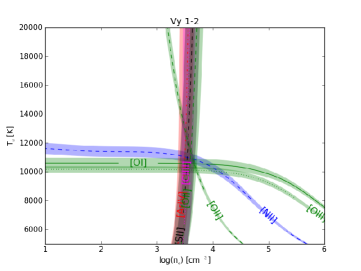
Figure 14: $\rm{T_{e}}$–$\rm{log(N_{e})}$ diagnostic plot for Vy 1–2.

3.3.2 Photo–ionisation modelling

In order to perform a more assiduous study on the ionisation structure of Vy 1–2, we constructed a photo–ionisation model using Cloudy (version 13.02; Ferland et al. 2013). Several atomic, ionic and molecular databases are used within Cloudy (e.g. Dere at al. 1997; Badnell et al. 2003; Badnell 2006, Landi et al. 2012; among others). The complete information can be found in Linkins et al. (2013) and Ferland et al. (2013).

Cloudy code uses as input parameters, (a) the energy distribution of the ionising radiation, (b) the luminosity of the central star and (c) some additional constraints that are usually estimated from the observed spectrum, which should as well be reproduced by the model such as the $\rm{T_{e}}$ and $\rm{N_{e}}$. Both parameters are required for determining the thermal balance of PNe. Because the configuration of the spectrograph does not include the lines of [O ii] 3726 Å and 3729 Å, [Ne iii] 3869 Å and 3968 Å, He ii 4686 Å, [Ar iii] 7135 Å, they were drawn from WLB05.

The model of Vy 1–2 was developed using the simplest set of assumptions (i) a blackbody approximation for the central star and (ii) a spherically symmetric nebula with constant density. The initial abundances of He, N, O, S, Ar and Cl were taken from our empirical analysis whereas Ne and C abundances from WLB05, and all of them were kept as free parameters, except C. Dust grains were also included in the model since they play an important role in the thermal balance of PNe. However, there is no information regarding the grain composition (no ISO spectra are available) and a mixture of Polycyclic Aromatic Hydrocarbons (PAHs; optical constants from Desert et al. 1990, Schutte et al. 1993, Li & Draine 2001; for more detail see Ferland et al. 2013) and astronomical graphite and silicate (Martin & Rouleau 1991; Laor & Draine 1993) with a constant dust–to–gas ratio, was adopted. The amount of PAH, graphite and silicate, grains were also kept as free parameters. Furthermore, the filling factor was kept as a free parameter in order to reproduce the observed $\rm{H\beta}$ flux.

Table 6: Total abundances, $\epsilon$(X)=log(n(X)/n(H))+12, of Vy 1–2.

$\epsilon$(X)	this work	this work	WLB05	Bar78b	Stan06	Solara
	(ICF)	(model)
He	11.04	11.03	11.03	10.98	11.23	10.93
C	$-$	8.08b	8.08b	$-$	$-$	8.43
O	8.66	8.91	8.70	8.79	8.46	8.69
N	8.13	8.42	8.06	8.03	7.90	7.83
S	6.80	7.37	6.78	6.98	$-$	7.12
Ne	$-$	8.11	8.00	8.19	7.81	7.93
Ar	6.28	6.39	6.25	$-$	5.84	6.40
Cl	5.22	5.31	$-$	$-$	$-$	5.50
log(N/O)	-0.53	-0.49	-0.64	-0.76	-0.56	-0.86
log(S/O)	-1.86	-1.54	-1.92	-1.81	$-$	-1.57
log(Ne/O)	$-$	-0.80	-0.70	-0.60	-0.65	-0.76
log(Ar/O)	-2.38	-2.52	-2.45	$-$	-2.62	-2.29
log(Cl/O)	-3.44	-3.60	$-$	$-$	$-$	-3.19

^a Asplund et al. 2009

^b C abundance was derived from collisionally excited lines. A higher C abundance of $\epsilon$(C)=8.98 was also derived from the optical recombination lines (WLB05). Vy 1–2 is a nebula with moderate high abundance discrepancy factors.

Given that C, O and N are the most important coolant elements in PNe, and they play a significant role in the thermal balance, small changes in their abundances can significantly affect the intensities of the emission lines of all elements. Hence, in order to get the best fit between the modelled and observed spectrum, we first varied the N and O abundances until the intensities of [N ii] 6584 Å and [O iii] 5007 Å emission lines were fitted. Then, regarding the other elements, we varied the abundances of the rest of elements (He, S, Ar and Cl) up to the point that the intensities of He ii 5876 Å, [S ii] 6716, 6731 Å, [Ar iv] 4712, 4740 Å and [Cl iii] 5517, 5538 Å lines, were also fitted. The modelled spectrum of Vy 1-2 is presented in Table 3 together with the observed spectrum. The mean difference between the observed and modelled intensities is $\sim$10% for the bright lines (S/N$>$5) and $\sim$20–30% for the fainter lines (S/N$<5$). The [K iv] 6101 Å and [Si ii] 5040 Å lines, as well as the stellar C ii 6461 Å, C iv 5801 and 5812 Å and the O iii 5592 Å lines, were not used to constrain the model.

As for the carbon, we assumed a constant abundance of log(C/H)+12=8.08, which was derived from the collisionally excited lines but it was not possible to get a good match of the CEL and ORL at the same time (very weak ORL), while the ionisation balance of C was far from the observed value. Assuming a higher C abundance (of 9.0), the model better predicts the ORL but overestimates the CEL. In addition to the blackbody stellar model, a H–deficient stellar atmosphere model for the ionizing source was also used. A good match between the modelled and observed spectrum could be obtained only for the case of high C abundance ($\epsilon$(C)$>$9).

In conclusion, whatever stellar atmosphere model was chosen for Vy 1-2, we did not fully reproduce the observed properties (e.g. the ionisation balance of the elements) to a satisfactory degree. In particular, the ionisation balance of all the elements is overestimated by the low C abundance model, whilst the higher C abundance model seems to produce an ionisation balances that matches better the observed ones. Also, our simple spherically symmetric shell geometry seems to be far from the real structure of the nebula, which as discussed in § 3.1 seems to have a bipolar structure or at least a significant deviation from a spherically symmetric morphology.

4 Discussion

4.1 Morpho–kinematic analysis

Vy 1–2 shows a high–speed component expanding with velocities up to 90–100  km s^-1, which is likely associated with the material in the faint bipolar lobes, with the eastern and western being blue– and red–shifted, respectively. Considering that these lobes are inclined by 10^∘ with respect to the line of sight and their projected distance on the sky is 3.6″ (measured from the eastern to the western lobe), we get a rough estimation of the nebula’s size along the polar axis of 20.4″ (r=10.2″). Given that the bipolar lobes have a de–projected radial expansion velocity of 90–100  km s^-1, their kinematic age is found to be 5200$\pm$750 years, for D=9.7 kpc.

A pair of knots is marginally detected in the HST [O iii] image, located at 11.5″ (knot S) and 14.5″ (knot N) from the central star. The projected expansion velocity of knot N differs from the $V_{\rm{sys}}$ of the nebula by 5  km s^-1. This converts to a de–projected radial velocity in a direction away from the central star of V=5/cos($\theta$)  km s^-1, where $\theta$ is the inclination angle of the knot to the line of sight. If we consider that the pair of knots is the result from the same ejection that formed the bipolar nebula (same age), its de–projected expansion velocity should be up to $\sim$130  km s^-1. Taking into account the projected velocity of knot N (5  km s^-1), as measured from the PV diagrams (Fig. 8), the inclination angle of the knots is found 89^∘ with the respect to the line of sight. This suggests a possible precession of the putative central star system and multiple ejection events leading to the formation of a bipolar nebula.

A single Gaussian was fitted to the emission line profiles of H$\alpha$, He ii, [N ii] and [O iii] and gave expansion velocities for the unresolved ring–like structure of 19$\pm$3  km s^-1, (23–25)$\pm$4  km s^-1, (8–9)$\pm$2  km s^-1 and 18$\pm$3  km s^-1, respectively. For V_exp=19  km s^-1and r=1.4″, we estimate the kinematic age of the ring–like structure $\sim$3500$\pm$500 years. This means that the ring–like structure was formed more recently than the bipolar lobes, which is not feasible. If, although, the inclination angle of the bipolar lobes is slightly higher of 15^∘, we get the same dynamical age for both component, ring–like and bipolar lobes, of 3500 years.

The velocity trend, on which the low–ionisation gas (e.g. [N ii]) expand slower than the high–ionisation gas–e.g. [O iii], He ii, is not consistent with a typical homologous expansion law, where their expansion velocity increases linearly with the distance from the central star. Despite the fact that $\rm{V_{[O{\sc\ III}]}}$ and $\rm{V_{He{\sc\ II}}}$ could be roughly considered the same within the uncertainties, the much lower $\rm{V_{[N{\sc\ II}]}}$ provides strong evidence for a non–homologous expansion. A small group of PNe (e.g. BD +30^∘3639, Akras & Steffen 2012; see also Medina et al. 2006) has been found to show this velocity trend. The central stars of those PNe are either [WR] or WEL–type stars (Medina et al. 2006). The acceleration of the inner zones of the nebula might be the result of strong, fast winds from a [WR] or WEL nucleus (Gesicki & Zijlstra 2003). The detection of the C ii 6461 Å, C iv 5801 and 5812 Å and O iii 5592 Å stellar lines in Vy 1–2 supports this scenario (see §4.3.2). Another possible scenario responsible for the acceleration of the inner nebular regions is a nova–type eruption of a close binary system. Akras & Steffen (2012) propose this mechanism in order to explain the morpho–kinematic characteristics of the young BD +30^∘3639 nebula.

4.2 Chemical analysis

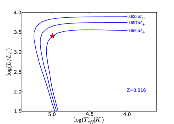
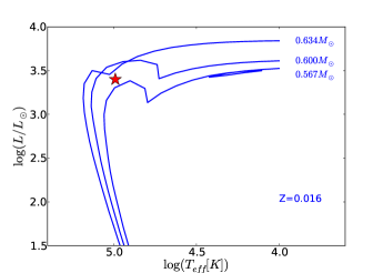
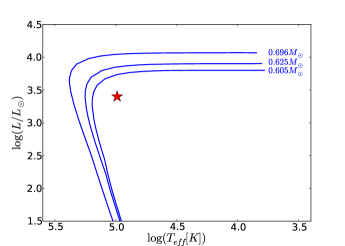
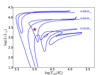
Figure 15: Hertzprung–Russell diagrams for hydrogen–burning (left panels) and helium–burning (right panels) models. Upper panels display the evolutionary tracks from Vassiliadis & Wood (1994) produced by ($\rm{M_{initial}}$, $\rm{M_{final}}$) = (1$\rm{M_{\odot}}$, 0.569$\rm{M_{\odot}}$), (1.5$\rm{M_{\odot}}$, 0.597$\rm{M_{\odot}}$) and (2$\rm{M_{\odot}}$, 0.633$\rm{M_{\odot}}$) for the hydrogen–burning model (left panel) and (1$\rm{M_{\odot}}$, 0.567$\rm{M_{\odot}}$), (1.5$\rm{M_{\odot}}$, 0.600$\rm{M_{\odot}}$) and (2$\rm{M_{\odot}}$, 0.534$\rm{M_{\odot}}$) for the helium–burning model (right panel). Lower panels display the evolutionary tracks from Blöcker (1995) produced by ($\rm{M_{initial}}$, $\rm{M_{final}}$) = (3$\rm{M_{\odot}}$, 0.605$\rm{M_{\odot}}$), (3$\rm{M_{\odot}}$, 0.625$\rm{M_{\odot}}$) and (4$\rm{M_{\odot}}$, 0.696$\rm{M_{\odot}}$) for the hydrogen–burning model (left panel) and (1$\rm{M_{\odot}}$, 0.524$\rm{M_{\odot}}$), (3$\rm{M_{\odot}}$, 0.625$\rm{M_{\odot}}$) and (5$\rm{M_{\odot}}$, 0.836$\rm{M_{\odot}}$) for the helium–burning model (right panel). The position of the central star of Vy 1–2 for a distance of 9.7 kpc is marked with a red star symbol.

The plasma parameters of Vy 1–2 such as T_e, N_e and chemical abundances were derived by means of the empirical methods and photo–ionisation modelling. Our best–fitting model provides a good approximation of the observed spectrum, except for the [O iii] 4959, 5007 Å doublet, and adds some constraints to the nebular and stellar properties of Vy 1–2. The predicted H$\beta$ flux is in a good agreement with the observed flux (see Table 3) with a filling factor equal to 0.44. The mean difference between the observed and modelled lines varies from 10% for the bright lines (S/N$>5$; the discrepancy in the [O iii] 4959, 5007 Å doublet is about 14%) to $\sim$20–30% for the fainter lines, S/N$<$5. Moreover the intensities of [O i] and [N i] neutral lines are underestimated. There are two possible scenarios for this: i) there is a large amount of neutral material around the nebula and/or ii) shock excitation of neutral lines close to the ionisation front may be significant. We can actually rule out the first scenario since the model predicts a density–bounded nebula whereas high expansion velocities up to 90–100  km s^-1 could favour the second scenario.

The total chemical abundances of Vy 1–2, for a blackbody stellar flux distribution, are listed in Table 6, which also includes those derived from previous studies, as well as the solar abundances, for direct comparison. The low He and N/O abundances imply a non Type–I nebula based on both Peimbert & Torres–Peimbert’s (1983) and Kingsburgh & Barlow (1994) classifications. The O abundance derived from the empirical ICF is found to be almost solar and close to the average value of non–Type I PNe (Bohigas 2008). Our best–fitting model predicts a somewhat higher value by 0.25 dex meaning that the star has not undergone the ON–cycle burning during the second dredge–up phase.

Given that Vy 1–2 is an O–rich nebula – log(C/O)=-0.62, WLB05; or log(C/O)=-0.83; our model – and the C abundance ($\epsilon$(C)=8.08) is lower than half of the solar (Asplund et al. 2009) as well as the average non–type I PNe values, the N enrichment must have occurred by the conversion of C to N, via the hot–bottom burning (HBB; CN–cycle). It is known from theoretical models of stellar nucleosynthesis that only the progenitor stars with masses $\geq$3 $\rm{M_{\odot}}$ undergo the $\rm{2^{nd}}$ dredge–up and HBB events (Karakas et al. 2009). This result is inconsistent with the low N/O abundance ratio (-0.53 (ICF), -0.48 (model)) and a low–mass progenitor star ($\leq$1 $\rm{M_{\odot}}$).

Unlike the single star evolutionary models, a close binary system can give such low N/O and C/O abundance ratios via the mass–transfer exchange (Iben & Tutukov 1993, De Marco 2009). Hf 2–2, NGC 2346 and Hb 12 are PNe that have confirmed close binary systems and low N/O and C/O values (see De Marco 2009). In a common envelope evolution, the AGB–phase may be significantly shorter than in a single star case resulting in the formation of an O–rich envelope (Izzard et al. 2006).

A comparison of the chemical abundance of Vy 1–2 with those derived from PNe with different types of nucleus (normal, WEL and [WR]) shows that the He abundance and N/O ratio better match with those from WEL–type nuclei while the O abundance with those from WEL– and [WR] types (Górny et al. 2009). As for the other elements, Ne matches those from WEL–type nuclei, Ar those from WEL– and normal–type nuclei, while Cl abundance is found to be significantly lower than those values derived by Gorny et al. (2009) for all types of nuclei, but closer to the solar value. In particular, the average abundance of Cl varies from 6.12 to 6.48, while we find $\epsilon$(Cl)=5.22 (ICF method) and 5.31 (photo–ionisation model). S abundance seems to match all types of nuclei due to the large difference between the ICF method ($\epsilon$(S)=6.80) and the photo–ionisation model ($\epsilon$(S)=7.37). This may be a consequence of the poor fit of the [S iii] 6312 Å emission line. The abundance uncertainties are $\sim$10% for the He and $\sim$20–30% for the rest of the elements.

It is worth mentioning here that Vy 1–2 has also been considered as a candidate halo PN due to its large distance from the Galactic plane ($\sim$500) and its high systemic velocity (-85$\pm$4  km s^-1) (Quireza et al. 2007). However, a comparison of its chemical abundances with those from Galactic disk and halo PNe (Otsuka et al. 2009) does not support this classification.

The best-fitting model of Vy 1–2, presented here, fails to reproduce the [O iii] 5007 Å and 4959 Å emission lines. The difference between the observed and modelled values is about 14%, similar to another PN with a WR–type central star as well as large abundance discrepancy factors (ADFs), NGC 1501 (Ercolano et al. 2004). We have to point out, though, that the emission line ratio [O iii] 5007/4363, which is an indicator of $\rm{T_{e}}$ of the nebula, is predicted with an accuracy better than 5%. The main causes of the model’s inability to reproduce the observed ionization balance and predict the bright [O iii] lines may be: i) the structure of the nebula, which is far from the spherically symmetric assumption, ii) the stellar continuum, where neither the blackbody nor an H–deficient stellar atmosphere model were able to reproduce all the observed data and/or iii) the dust composition, which seems to play a crucial role in this objects, but no information is available for Vy 1-2.

The large ADFs found in Vy 1–2 for O⁺⁺, N⁺⁺, C³⁺, C⁺⁺ and Ne⁺⁺ are of 6.17, 11.8, 14.0, 9.27 and 13.8, respectively (see WLB05) and could indicate the possible presence of cold H–deficient clumps in the nebula, which may also hinder the results of our model This possibility is, however, beyond the scope of this paper.

4.3 Central star

4.3.1 Evolutionary status

Our simple blackbody stellar model predicts a luminosity $\rm{\log(L/L_{\odot})}$=3.40 and an effective temperature $\rm{T_{eff}}$=98 kK, for D=9.7 kpc. For a distance of 7.8 kpc, we obtain $\rm{\log(L/L_{\odot})}$=3.21 in good agreement with those values reported by Stangellini et al. (2002) and Phillips (2003). Figure 15 portrays the positions of Vy 1–2’s central star in the HR diagram, for a distance of 9.7 kpc. The theoretical evolutionary tracks plotted are the hydrogen–burning (left panel) and helium–burning (right panel) models from Vassiliadis & Wood (1994; upper panels) and (Blöcker 1995; lower panels). In Vassiliadis and Wood’s models, the central star corresponds to a progenitor mass of 1 $\rm{M_{\odot}}$ and a core mass of 0.569 $\rm{M_{\odot}}$ (hydrogen–burning ) and 0.567 $\rm{M_{\odot}}$ (helium–burning). The timecales from these evolutionary tracks are significantly higher than the kinematic age of the nebula with 26000 years and 41000 years for the hydrogen– and helium–burning respectively.

In Blöcker’s models, the evolutionary track for a very late thermal pulse (VLTP) (lower, right panel) implies a progenitor star of 3 $\rm{M_{\odot}}$ and a core mass of 0.625 $\rm{M_{\odot}}$. Even though the timescale of the former evolutionary track is still higher than the kinematic age of the nebula, by a factor of $\sim$2, it is closer to the observed value. The scenario of a close companion and mass–transfer exchange would be able to explain the rapid evolution of the star. Unlike the 1 $\rm{M_{\odot}}$ low mass star, a 3 $\rm{M_{\odot}}$ progenitor star can go through the HBB effect during the 2^nd dredge–up phase resulting in enhancement of N and depletion of C. The detection of the C ii 6461 Å, the doublet C iv$\lambda$ $\lambda$ 5801, 5812 and the O iii 5592 Å stellar lines emitted from a hydrogen–deficient star supports the VLTP scenario.

Our new distance value indicates that Vy 1–2 is a distant nebula (9.7 kpc) and provides a much better agreement between the kinematic age of the nebula and the evolutionary age of the central star.

4.3.2 [WR] or WEL type nucleus?

Apart from the detection of the common nebular emission lines, weak stellar emission lines such as C ii 6461 Å, C iv 5801 and 5812 Å and O iii 5592 Å were also detected for the first time in this nebula in our very deep spectra (Table 7). Their line profiles are shown in Fig. 16. There are two groups of stars with emission lines of highly ionised He, C, O and N: [WR] (Crowther 2008) and WELS stars (Tylenda et al. 1993). Although, both classes exhibit the same emission lines (e.g C iv doublet 5801 and 5812 Å and [C iii] 5696 Å), the former show much broader lines profiles and stronger intensities than the latter due to the fast and strong stellar winds.

Based on the classification scheme of Acker & Neiner (2003) and the C ii/C iv and O iii/C iv line ratios, the central star of Vy 1–2 is classified as a late–type star ([WRL]). On the other hand, the absence of the [C iii] 5696 Å line (see WLB05) in conjunction with the detection of the C iv doublet, N iii and C iii–iv 4650 Å lines, also suggest a WEL–type nucleus. Therefore, new high–resolution observations are required in order to confirm the spectral type of this star.

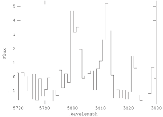
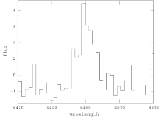
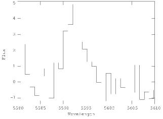
Figure 16: Part of the spectrum of Vy 1–2, in which the faint stellar lines C iv $\lambda$  $\lambda$ 5801, 5812 Å, C ii 6461 Å and O iii 5592 Å are seen (in units of $10^{-14}$ erg $\rm{s^{-1}}$ $\rm{cm^{-2}}$).

4.4 Infrared properties and SED

Vy 1-2 is also a strong infrared emitter indicating the presence of significant amount of dust. Thus far, no one had studied the infrared emission and dust properties of this compact nebula. For this study, we used infrared data from 2MASS, IRAS (IRAS 17524+2800), AKARI and WISE data archives. The data cover a wavelength range from the near– to the far–infrared.

Table 7: Stellar emission lines of Vy 1–2

Line (Å)	F($\lambda$)a	S/N
O iii 5592	0.08	3.0
C iv 5801	0.12	3.0
C iv 5812	0.11	3.0
C ii 6461	0.09	3.0

^a Relative to the nebular H$\beta$=100

The spectral energy distribution (SED) of Vy 1-2 is presented in Fig. 17 and displays a double–peaked profile. One peak lies at the optical wavelength due to the hot central star (100,000 K) of the nebula and the second one at  30–40 $\mu$m implying the presence of a cold dusty circumstellar shell with a temperature of $\sim$100–150 K. Vy 1–2 may also exhibit a small K–band excess, associated either with a hot dust component or the emission from a cool ($\sim$2000 K) unresolved companion.

The all–sky Wide–Field Infrared Survey Explorer (WISE) observed Vy 1-2 in four photometric bands at 3.35 $\mu$m, 4.6 $\mu$m, 11.6 $\mu$m and 22.1 $\mu$m (W1 through W4, respectively; Fig. 18). Because of the low angular resolution in these bands (6.1″, 6.4″, 6.5″and 12″, respectively; Wright et al. 2010), Vy 1-2 remains unresolved. It is worth mentioning here that W1 and W2–band images unveil the presence of a seemingly collimated outflow in the same direction as the NW knot (PA=310^∘). An arrow in Figure 18 indicates the position of the collimated structure. Despite the W3–band having a similar angular resolution to those of W1 and W2 bands, the collimated structure can not be discerned.

By scrutinizing the DSS images for Vy 1-2, we discover the presence of a very faint starlike object in the same direction as the outflow and in the same position as the NW knot ($\sim$14″ away from the central star). The detection of this field star in the DSS IR band, as well as in the W1 and W2-bands but not in the W3-band, implies a very cold star with a temperature of $\sim$2000 K. Note that the seemingly halo observed in the W3 and W4 band images (panels (c) and (d) in Fig. 18) is not a real structure since it is also apparent around the bright field stars.

WISE bands, encompass the dust continuum and several features attributed to PAH features at 3.3 $\mu$m, 8.6 $\mu$m, 11.3 $\mu$m, 12.7 $\mu$m and 16.4 $\mu$m, silicate dust features at 9.7 $\mu$m and 18 $\mu$m as well as high excitation nebular lines (e.g. [S vi], [Ne iv] and [Ne v]). However, ISO spectra are not available, prohibiting any further investigation on the dust composition. Nevertheless, the detection of single ionised recombination C lines (C ii 6578 Å and 6581 Å) may suggest the presence of C–rich dust. The large excess in the W3 and W4 bands may also be associated with the presence of silicate dust features. The SwSt 1 nebula exhibits these C lines as well as the silicate dust feature at 10 $\mu$m (De Marco et al. 2001). A double–dust chemistry (O– and C–rich) is observed in PNe with [WR] or WEL type central stars, probably due to the VLTP that turn the central stars from O–rich to C–rich.

In order to constrain the dust emission, we used the aforementioned broad–band infrared fluxes. The best–fitting SED to the infrared data was possible only assuming a C–rich dust model. Figure 17 displays the modelled SED of Vy 1–2. The PAHs are $\sim$5.7 times more abundant (by mass) than the silicates and the dust-to-gas ratio equal to 1.05$\times$10^-2. The total mass of the nebula and the dust mass are  0.08 M$\odot$ and 8.4 10^-4 M$\odot$, respectively. The high uncertainty of Vy 1–2’s distance implies as well high uncertainties in these masses. This result is consistent with the scenario of a hydrogen deficient star and dual–dust chemistry. Interestingly, the ionized gas indicates an O-rich nebula (C/O$<$1), whilst the dust composition is C-rich. One possible explanation, as recently proposed by Guzmán–Ramirez et al. (2014), is the formation of PAHs from the photo–dissociation of CO in a torus, such as the bright ring–like structure in Vy 1-2, whereas the dust in the main nebula remains O–rich. Moreover, a recent change of the stellar surface chemistry due to the second dredge–up of C, as has been proposed to explain the dual–dust chemistry in the young PN BD +3036 (Guzmán–Ramirez et al. 2015), can also provide a plausible explanation for Vy 1–2 as well. We have to stress out though there is no available infrared spectroscopic data for Vy 1–2 and our analysis is based on the results from our best-fitting photo–ionisation model using the broad–band infrared fluxes.

In summary, a careful look at the modelled SED reveals a lower flux in the infrared H–band, indicating that this measurement may be underestimated and the seemingly K-band excess is not really an excess associated with the presence of a cold companion as previously mentioned.

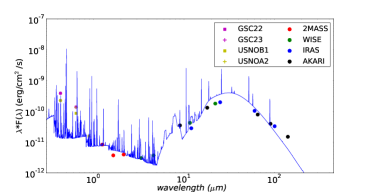
Figure 17: The observed and modelled SED of Vy 1–2 in the wavelength range from 0.43 to 140 $\mu$m. The data are from GSC2.2, GSC2.3, USNOB1, USNOB2, 2MASS, AKARI and WISE surveys.

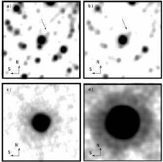
Figure 18: WISE images of Vy 1–2 in four bands: a) 3.35 $\mu$m, b) 4.6 $\mu$m, c) 11.6 $\mu$m and d) 22.1 $\mu$m. The arrows indicate the position of the field star. The field of view is 180″$\times$180″. North is up and East is to the left.

5 Conclusions

The main conclusions of this work are summarized as follow:

1) Vy 1–2 presents a bipolar structure, seen almost pole–on. The bipolar lobes expand with velocities up to 90–100  km s^-1, whereas the bright, inner ring–like structure shows lower expansion velocities of V_Hα =19  km s^-1, V${}_{\rm{He{\sc\ II}}}$ =23–25  km s^-1, $\rm{V_{[N{\sc\ II}]}}$=8–9  km s^-1 and $\rm{V_{[O{\sc\ III}]}}$=18  km s^-1. These velocities indicates a possible acceleration process of the inner nebular regions, which may be associated with the strong/fast stellar wind from a [WR] or WEL nucleus. The kinematic age of the nebula is $\sim$3500 years for a distance of 9.7 kpc.

2) A pair of knots is also apparent along P.A.=305^∘, located at 11.5″ and 14.5″ and moving perpendicular to the line of sight. Assuming that they were formed approximately at the same time as the nebula, we estimated their velocities up to a value of 130$\pm$15  km s^-1.

3) Vy 1–2 is apparently an O–rich, non–type I nebula (log(C/O)=-0.58 (ICF) and -0.83 (model), -0.53$\leq$log(N/O)$\leq$-0.49). Compared to solar abundances, O was found to be solar, C subsolar and it is enriched in N. The HBB CN–cycle must have occurred in order to explain these abundances, implying a progenitor star with initial mass $\geq$3 M_⊙.

4) None of the stellar ionizing continua used in our photo–ionisation model (blackbody or H–deficient) were able to reproduce the observed ionisation balance of the elements. The spherical symmetry asssumed for the nebula may be far from the real structure of Vy 1–2, and a more sophisticated 3–D bi–abundance model is required for the proper study of its ionisation structure.

5) The low C/O and N/O abundance ratios of Vy 1–2 can not be attained by single star evolutionary models, and a post–common envelope binary system seems a more plausible scenario. The N enhancement can be explained by the binary interaction via mass–transfer exchange.

6) A very late thermal pulse may also have occurred resulting in the formation of a H–deficient star. The detection of the C ii 6461 Å, the C iv$\lambda$ $\lambda$ 5801, 5812 doublet and the O iii 5592 Å stellar lines supports this scenario. The timescale of VLTP evolutionary track for a 3 M_⊙ progenitor star is consistent with the kinematic age of the nebula.

7) Vy 1–2 is found to be very bright at the mid–IR indicating large amount of dust. Its SED shows a double–peaked profile with one peak at 30–40 $\mu$m which implies a circumstellar envelope with a temperature of $\sim$100 K. The C/O$<$1 abundance ratio of the ionised gas indicates a O–rich nebula, whilst our best–fitting model predicts a C–rich dust, with PAHs being almost 5 times more abundant (by mass) than silicates. A possible interpretation of this result may be the formation of PAHs in a torus due to the photo–dissociation of CO and the formation of silicates in the main nebula or a recent change of stellar chemical composition due to the second dredge–up of C.

References

- Acker (2003) Acker A., Neiner C., 2003, A&A, 403, 659.
- Akras (2012) Akras S., Steffen W., 2012, MNRAS, 423, 925.
- Asplund (2009) Asplund M., Grevesse N., Sauval A. J., Scott P., 2009, ARA&A, 47, 481.
- Badnell (2003) Badnell N. R., O’Mullane M. G., Summers H. P., Altun Z., Bautista M. A., Colgan J., Gorczyca T. W., Mitnik D. M., Pindzola M. S., Zatsarinny O., 2003, A&A, 406, 1151.
- Badnell (2006) Badnell N. R., 2006, ApJS, 167, 334.
- Barker (1978) Barker T., 1978a, AJ, 219, 914.
- Barker (1978) Barker T., 1978b, AJ, 220, 193.
- Benjamin (1999) Benjamin R. A., Skillman E. D., Smits D. P., 1999, ApJ, 514, 307.
- Blocker (1995) Blöcker T., 1995, A&A, 299, 755.
- Bohigas (2001) Bohigas J., 2001, RMxAA, 37, 237.
- Bohigas (2008) Bohigas J., 2008, ApJ, 674, 954.
- Bohigas (2015) Bohigas J., Escalante V., Rodríguez M., Dufour R. J., 2015, MNRAS, 447, 817B.
- Boumis (2006) Boumis P., Akras S., Xilouris E. M., et al., 2006, MNRAS, 367, 1551B.
- Boumis (2006) Boumis P., Paleologou E. V., Mavromatakis F., Papamastorakis J., 2003, MNRAS, 339, 735B.
- Bryce (1999) Bryce M., Mellema G., 1999, MNRAS, 309, 731.
- Butler (1989) Butler K., Zeippen C. J., 1989, A&A, 208, 337.
- Cahn (1971) Cahn J. H., Kaler J. B., 1971, ApJS, 22, 319C.
- Cahn (1992) Cahn J. H., Kaler J. B., Stanghellini L., 1992, A&AS, 94, 399.
- Calavis (1995) Galavis M. E., Mendoza C., Zeippen C. J., 1995, A&A Supp., 111, 347.
- Condon (1998) Condon J. J., Kaplan D. L, 1998, ApJS, 117, 361.
- Crowther (2008) Crowther P. A., 2008, ASPC, 391, 83.
- Dere (1997) Dere K. P., Landi E., Mason H. E., Monsignori Fossi B. C., Young P. R., 1997, A&AS, 125, 149.
- DeMarco (2001) De Marco O., Crowther P. A., Barlow M. J., et al., 2001, MNRAS, 328, 527D.
- DeMarco (2008) De Marco O., Hillwig Todd C., Smith A. J., 2008, AJ, 136, 323D.
- DeMarco (2009) De Marco O, 2009, PASP, 121, 316D.
- Depew (2011) Depew K., Parker Q. A., Miszalski B., De Marco O., Frew D. J., Acker A., Kovacevic A. V., Sharp R. G., 2011, MNRAS, 414, 2812.
- Desert (1990) Desert F.-X., Boulanger F., Puget J. L. 1990, A&A, 237, 215.
- Ercolano (2004) Ercolano B., Wesson R., Zhang Y., Barlow M. J., De Marco O., Rauch T. and X.-W. Liu X. -W., 2004, MNRAS, 354, 558.
- Ferland (2013) Ferland G. J., Porter R. L., van Hoof P. A. M., Williams R. J. R., Abel N. P., Lykins, M. L., Shaw, G., Henney, W. J., Stancil, P. C., 2013, RMxAA, 49, 137
- Flores-Durán (2014) Flores–Durán S. N., Peña M., Hernández–Martínez L., García–Rojas J., Ruiz M. T., 2014, A&A, 568A, 82F.
- Fitzpatrick (1999) Fitzpatrick E. L., 1999, PASP, 111, 63.
- Frew (2013) Frew D. J., Bojičić I. S., Parker Q. A., 2013, MNRAS, 431, 2F.
- Frew (2010) Frew D. J., Parker Q. A., 2010, APN5 Conf. Proc., Ebrary, 33, arXiv:1010.5003.
- Gesicki (2003) Gesicki K., Zijlstra A. A., 2003, MNRAS, 338, 347.
- Girard (2007) Girard P, Koppen J., Acker A,. 2007, 463, 265.
- Gorny (2009) Górny S. K., Chiappini C., Stasińska G., Cuisinier F., 2009, A&A, 500, 1089.
- Gurzadian (1988) Gurzadian G. A., 1988, Ap&SS, 149, 343.
- Guzman (2014) Guzman–Ramirez L., Lagadec E., Jones D., Zijlstra A. A., Gesicki K., 2014, MNRAS, 441, 364G.
- Guzman (2015) Guzman–Ramirez L., Lagadec E., Wesson R., et al. 2015, MNRAS, 451L, 1G.
- Hamuy (1992) Hamuy M., Walker A. R., Suntzeff N. B., Gigoux P., Heathcote S. R., Phillips M. M., 1992, PASP, 104, 533.
- Harman (2004) Harman D. J., Bryce M., López J. A., Meaburn J., Holloway A. J., MNRAS, 2004, 348, 1047
- Hyung (1997) Hyung S., Aller H. L., 1997, MNRAS, 292, 71.
- Hyung (2000) Hyung, S., Aller, L. H., Feibelman, W. A., Lee, W. B., de Koter, A. 2000, MNRAS, 318, 77.
- Jones (2014) Jones D., Boffin H. M. J., Miszalski B., Wesson R., Corradi R. L. M., Tyndall A. A., 2014, A&A, 562A, 89J.
- Iben (1993) Iben I., Tutukov V. A., 1993, ApJ, 418, 343.
- Izzard (2006) Izzard R. G., Dray L. M., Karakas A. I., Lugaro M., Tout C. A., 2006, A&A, 460, 565.
- Karakas (2009) Karakas A. I., van Raai M. A., Lugaro M., Sterling N. C., Dinerstein H. L., 2009, ApJ, 690, 1130.
- King (1994) Kingsburgh R. L., Barlow M. J., 1994, MNRAS, 271, 257.
- Krist (2011) Krist J. E., Hook R. N., Stoehr F., 2011, SPIE, 8127E, 0JK.
- Kwok (2010) Kwok S., 2010, PASA, 27, 174.
- Lagadec (2011) Lagadec E., et al. 2011, MNRAS, 417, 32.
- Laor (1993) Laor A., Draine B. T., 1993, ApJ, 402, 441.
- Landi (2012) Landi E., Del Zanna G., Young P. R., Dere K. P., Mason H. E., 2012, ApJ, 744, 99.
- Lee (2001) Lee H.–W., Kang Y.–W., Byun Y.–I., 2001, ApJ, 551L, 121.
- Lennon (1994) Lennon D. J., Burke V. M., 1994, A&AS, 103, 273.
- Li (2001) Li A., Draine B. T., 2001, ApJ, 554, 778.
- Liu (2000) Liu X.-W., Storey P. J., Barlow M. J., Danziger I. J., Cohen M. and Bryce M., 2000, MNRAS, 312, 585.
- Liu (2001) Liu X.-W., Luo S.-G., Barlow M. J., Danziger I. J. and Storey P. J., 2001, MNRAS, 327, 141.
- Lopez (2012) López J. A., Richer M. G., García–Díaz Ma. T., Clark D. M., Meaburn J., Riesgo H., Steffen W., & Lloyd, M., 2012, RevMexAA, 48, 3.
- Luridiana (2012) Luridiana V., Morisset C., Shaw R. A., 2012, IAUS, 283, 422.
- Lykins (2013) Lykins M. L., Ferland G. J., Porter R. L. van Hoof P. A. M., Williams R. J. R., Gnat O., 2013, MNRAS, 429, 3133L.
- Maciel (1984) Maciel, W. J., 1984, A&AS, 55, 253.
- Manchado (1996) Manchado A., Guerrero M. A., Stanghellini L., & Serra–Ricart M. 1996, The IAC morphological catalogue of northern Galactic planetary nebulae.
- Manchado (2011) Manchado A., García–Hernández D. A., Villaver E., Guironnet de Massas J., 2011, ASPC, 445, 161.
- Martin (1991) Martin P. G., Rouleau F. 1991, in Extreme Ultraviolet Astronomy, ed. R. F. Malina & S. Bowyer (New York: Pergamon), 341.
- McKenna (1996) McKenna F. C., Keenan F. P., Kaler J. B., Wickstead A. W., Bell K. L., Aggarwal K. M., 1996, PASP, 108, 610.
- Meaburn (2003) Meaburn J., López J. A., Gutiérrez L., Quiróz F.; Murillo J. M., Valdéz, J., Pedrayez M., 2003, RMxAA, 39, 185.
- Meaburn (2005) Meaburn J., Boumis P., López J. A., Harman D. J., Bryce M., Redman M. P., Mavromatakis F., 2005, MNRAS, 360, 963M.
- Medina (2006) Medina S., Peña M., Morisset C., Stasińska G.,2006, RMxAA, 42, 53.
- Meixner (1999) Meixner M., et al., 1999, ApJS, 122, 221.
- Mendoza (1982) Mendoza C., Zeippen C. J., 1982, MNRAS, 198, 127a.
- Mendoza (1982) Mendoza C., Zeippen C. J.,1982, MNRAS, 199, 1025b.
- Mendoza (1983) Mendoza C., 1983, ”Planetary Nebulae”, 143.
- Mennickent (2008) Mennickent R., Greiner J., Arenas J., Tovmassian G., Mason E., Tappert C., Papadaki C., MNRAS, 2008, 383, 845.
- Miszalski (2009) Miszalski B., Acker A., Parker Q. A., Moffat A. F. J., 2009, A&A, 505, 249.
- Miszalski (2008) Miszalski B., Parker Q. A., Acker A, Birkby J. L., Frew D. J., Kovacevic A., 2008, MNRAS, 384, 525.
- McNabb (2013) McNabb I. A., Fang X., Liu X.–W., Bastin R. J., Storey P. J., 2013, MNRAS, 428, 3443M.
- Otsuka (2009) Otsuka M., Hyung S., Lee S.–J., Izumiura H., Tajitsu A., 2009, ApJ, 705, 509O.
- Parker (2006) Parker Q. A., et al., 2006, MNRAS, 373, 79.
- Peimbert (1983) Peimbert M., Torres–Peimbert S., 1983, in Flower D. R., ed., IAU Symp. 103, 233.
- Phillips (1998) Phillips J. P., A&A, 1998, 340, 527.
- Phillips (2003) Phillips J. P., 2003, MNRAS, 344, 501.
- Phillips (2011) Phillips J. P., Márquez–Lugo R. A., 2011, RMxAA, 47, 83.
- Pradhan (1976) Pradhan A. K., 1976, MNRAS, 177, 31.
- Quireza (2007) Quireza C., Rocha–Pinto H. J., Maciel W. J., 2007, A&A, 475, 217Q.
- Lario (2012) Ramos–Larios G., Guerrero M. A., Vázquez R., Phillips J. P., 2012, MNRAS, 420, 1977.
- Ramsbottom (1996) Ramsbottom C. A., Bell K. L., Stafford R. P., 1996, ADNDT, 63, 57.
- Sabadin (1984) Sabbadin F., Gratton R. G., Bianchini A., Ortolani S., 1984, A&A, 136, 181S.
- Sabin (2014) Sabin L., Parker Q. A., Corradi R. L. M., et al., 2014, MNRAS, 443, 3388S.
- Sahai (1999) Sahai R., Zijlstra A., Bujarrabal V., Hekkert Te Lintel P., AJ, 1999, 117, 1408.
- Sahai (2011) Sahai R., Morris M. R., Villar G. G., 2011, AJ, 141, 134.
- Schneider (1983) Schneider S. E., Terzian Y., Purgathofer A., Perinotto M., 1983, ApJS, 52, 399.
- Schutte (1993) Schutte W. A., Tielens A. G. G. M., Allamandola L. J. 1993, ApJ, 415, 397.
- Shaw (1994) Shaw, R. A., Dufour, R. J., 1994, ASPC, 61, 327.
- Seaton (1979) Seaton M. J., 1979, MNRAS, 187, 73.
- Stanghellini (2006) Stanghellini L., Guerrero M A., Cunha K, Manchado A., Villaver E., 2006, ApJ, 651, 898.
- Stanghellini (2002) Stanghellini L., Villaver E., Manchado A., Guerrero M. A., 2002, ApJ, 576, 285.
- Steffen (2011) Steffen W., Koning N., Wenger S., Morisset C., Magnor M., 2011, IEEE Transactions on Visualization and Computer Graphics, 17, 454.
- Soker (1994) Soker N., Livio M., 1994, ApJ, 421, 219.
- Tylenda (1993) Tylenda R., Acker A., Stenholm B., 1993, A&AS, 102, 595.
- Vassiliadis (1994) Vassiliadis E., Wood P. R., 1994, ApJS, 92, 125.
- Vaytet (2009) Vaytet N. M. H., Rushton A. P., Lloyd M., López J. A., Meaburn J., OB́rien T. J., Mitchell D. L., Pollacco D., 2009, MNRAS, 398, 385.
- Verner (1996) Verner D. A., Verner E. M., Ferland G. J., 1996, ADNDT, 64, 1.
- Weinberger (1989) Weinberger R., 1989, A&AS, 78, 301.
- Wesson (2005) Wesson R., Liu X.-W., Barlow M. J., 2005, MNRAS, 362, 424.
- Wiese (1996) Wiese W. L., Fuhr J. R., Deters T. M., 1996, JPCRD, Monograph 7.
- Wright (2010) Wright E. L., Eisenhardt P. R. M., Mainzer A. K., 2010, AJ, 140, 1868W.
- Zeippen (1987) Zeippen C. J., Butler K., Le Bourlot J., 1987, A&A, 188, 251.