Competition of Lattice and Basis for Alignment of Nematic Liquid Crystals

Abstract

Due to elastic anisotropy, two-dimensional patterning of substrates can promote weak azimuthal alignment of adjacent nematic liquid crystals. Here, we consider how such alignment can be achieved using a periodic square lattice of circular or elliptical motifs. In particular, we examine ways in which the lattice and motif can compete to favor differing orientations. Using Monte Carlo simulation and continuum elasticity we find, for circular motifs, an orientational transition depending on the coverage fraction. If the circles are generalised to ellipses, arbitrary control of the effective alignment direction and anchoring energy becomes achievable by appropriate tuning of the ellipse motif relative to the periodic lattice patterning. This has possible applications in both monostable and bi-stable liquid crystal device contexts.

I Introduction

Surface anchoring, the promotion of a desired liquid crystal (LC) orientation at a surface (Jerome, 1991), remains an important problem in applications because precise tuning of anchoring parameters is often necessary for optimal device performance (Spencer and Care, 2006). Patterning the surface with a spatially varying preferred orientation is an attractive route to create alignment layers with desired anchoring properties because both the effective anchoring strength and its orientation or easy axis can be altered by adjusting geometric features of the pattern (Kondrat et al., 2003; Barbero et al., 1992). Additionally, surfaces of appropriate symmetry (Anquetil-Deck et al., 2012) may promote multiple stable easy axes leading to bistable devices (Kim et al., 2001; Yi et al., 2008; Yoneya et al., 2002; Lee and Clark, 2001). Bistability is desirable (Kim et al., 2002; Stalder and Schadt, 2003; Bryan-Brown, 2000; Kitson and Geisow, 2002) both for reduced power consumption and improved addressing of hi-resolution displays. Beyond displays, patterned LC systems are promising candidates as biosensors (Hwang and Rey, 2006; Lowe et al., 2010) and photonic devices (Ruan et al., 2003; Wei et al., 2009).

Many methods exist to achieve patterning, encompassing both topographical and chemical approaches. These include mechanical rubbing (Bechtold and Oliveira, 2005; Varghese et al., 2004), photolithography (Bechtold and Oliveira, 2005; Schadt et al., 1992; Stalder and Schadt, 2003), scribing with an atomic force microscope (AFM) (Kim et al., 2002; Lee et al., 2004), microcontact printing of self-assembled monolayers (SAMs) (Gupta and Abbott, 1997; Cheng et al., 2000; Prompinit et al., 2010; Zheng et al., 2013), and topographic surface features (Liu et al., 2012). Since mechanical methods, such as rubbing, result in unwanted scratches or debris on the surface (Park and Park, 2008), and many methods do not scale well to high-volume manufacturing (Zheng et al., 2013), SAMs have received much attention in recent years. Certain experimental methods show control over the azimuthal director angle as well as the polar anchoring angle (Bechtold and Oliveira, 2005; Wilderbeek et al., 2003) - this is the focus of the work presented in this paper.

Striped surfaces, incorporating alternating regions preferring planar and vertical alignment, have been well studied (Atherton and Sambles, 2006; Atherton et al., 2009; Atherton, 2010; Ledney and Tarnavskyy, 2011; Kondrat et al., 2005; Yi and Clark, 2013). For this pattern, the polar angle of the bulk LC is controlled by the average polar easy axis on the surface; the azimuthal alignment has an energy minimum aligned parallel or perpendicular to the stripe orientation, depending on the ratio of the elastic constants (Atherton and Sambles, 2006). Square checkerboard lattices are more complicated: an anchoring transition occurs in which the liquid crystal aligns with the lattice vectors for relatively strong surface anchoring, but switches to the diagonal for very weak anchoring (Anquetil-Deck et al., 2012). Finally, both polar and azimuthal control over the bulk LC director orientation may be achieved with a rectangular checkerboard lattice. In this arrangement, certain rectangle ratios and anchoring strengths combine to shift the preferred director azimuthal angle from alignment with a rectangle edge to alignment diagonally across the rectangle (Anquetil-Deck et al., 2013).

For substrates constructed from squares or rectangles, the pattern element determines the symmetry and periodicity of the patterning. It is, however, straightforward to break this coupling by resorting to non-space-filling pattern basis motifs, such as circles or ellipses, and arranging these on a periodic lattice. Importantly, this approach provides a systematic approach by which to introduce the additional parameters needed to achieve truly independent control of polar and azimuthal anchoring angles and, so, set these at arbitrary target values.

In this paper, we use a continuum approach to determine the ground state of a liquid crystal in contact with a surface formed of a square lattice of circular or elliptical motifs. From this, we identify scenarios for which the basis symmetry and the lattice symmetry may favor different alignments. This yields bistable configurations which are free from the constraints that pertain for square or rectangular motifs. The paper is organized as follows: Monte Carlo simulation results with circle patterns are presented in section II. In section III, an analytical continuum model is constructed for this arrangement with the simplifying assumption that the director lies at a constant azimuthal angle. We also construct a numerical model that relaxes this assumption. Brief conclusions are presented in section IV.

II Simulations

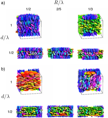
Figure 1: Snapshots of Monte Carlo simulations of a nematic confined between periodically patterned circles. (a) Vertical circles on planar background for different values of thickness $d$ and circle radius $R$. (b) Planar circles on vertical background for $d/\lambda=1/2$; the views show slices taken through the box mid-plane.

The combination of Monte Carlo (MC) simulations and continuum theory has proven synergistic in previous studies (Anquetil-Deck et al., 2012, 2013) because the alignment induced by a particular pattern depends dramatically on the length scales present: MC probes alignment around patterns at the order of a few molecular lengths while continuum theory permits modeling up to device scales.

To gain an initial understanding of the effect of circle patterns on the adjacent nematic, we therefore first performed Monte Carlo simulations as described fully in (Anquetil-Deck et al., 2012). Briefly, particle-particle interactions are modeled with the hard Gaussian overlap potential (HGO) and particle-wall interactions are modeled with the hard needle-wall (HNW) potential, where a hard axial needle of length $\sigma_{0}k_{s}$ is placed at the centers of particles of short diameter $\sigma_{0}$. By adjusting the needle length, both vertical ($k_{s}\leq 1)$ and planar alignment ($k_{s}>2$) can be achieved.

Here, simulations of HGO particles of aspect ratio $\kappa=3$ were performed subject to confinement between two circle-patterned substrates separated by a distance $d$. Periodic boundaries were imposed in the $x$ and $y$ directions. Sharp boundaries were imposed between vertical and planar regions, needle lengths being specified in each region as described above. Particle configurations were initialized at low density and uniformly compressed in the $x$ and $y$ until orientational order was established. The corresponding in-plane box-length, $\lambda$, then set the effective lattice periodicity of the chosen circular motif. An equilibration run of $N=500,000$ MC sweeps was conducted at each density, followed by a production run of a further $N$ sweeps.

Representative snapshots are displayed in Fig. 1(a) for vertical circles on a planar background; corresponding plots for the reverse case are in Fig. 1(b). For $d=\lambda=4\kappa\sigma_{0}$, the orientational ordering of the particles at the center of the film can be seen to depend on $R$, the radius of the circle. If $d\simeq\lambda$, an anchoring transition occurs with decreasing $R$. For large $R$, the film follows the alignment of the particles in the circle be that planar or vertical. However, a transition occurs with decreasing $R$, after which the orientation in the film becomes dictated by the pattern outside the circle. This behavior is observed for both vertical-on-planar and planar-on-vertical surfaces and essentially mimics that seen for other patterned films - the film orientation is dominated by the majority surface component.

For thinner cells, where $d=\lambda/2$; the nematic follows the pattern throughout the vertical distance for all values of $R$ studied. This is similar to the “bridging” behavior observed in rectangular patterned systems (Anquetil-Deck et al., 2012, 2013). For the planar-on-vertical case [Fig. 1(b)], the particle orientation on the top and bottom substrates at a vertical-planar boundary is particularly interesting, because the here the particles tend to align parallel to the boundary causing azimuthal distortion of the liquid crystal.

A more subtle azimuthal transition is also apparent, however, from careful study of vertical on planar systems. As illustrated in Fig. 2, the preferred azimuth of the planar region is also dependent on $R$. Specifically, for larger circles particles in the in-plane region aligned along the box $x$ and $y$-axes, whereas at smaller $R$ they picked out the box diagonal. It is this azimuthal transition that we focus on in the remainder of this paper.

Figure 2: Apparent orientational anchoring transition. a) Top configuration for vertical on planar circles with $R/\lambda=1/3$ and $d/\lambda=1$. b) Top configuration for $R/\lambda=1/4$.

III Continuum Model

We now turn to the continuum analysis. The LC orientation is characterized by a director field,

$$\mathbf{n}=(\cos\theta\sin\phi,\cos\theta\cos\phi,\sin\theta),$$ (1)

where $\theta$ is the zenithal angle and $\phi$ is the azimuthal angle. The free energy of the LC will be given by the Frank free energy

$$F = \frac{1}{2}\int d^{3}\!x\,[K_{1}(\nabla\cdot\mathbf{n})^{2}+K_{2}(\mathbf{n}\cdot\nabla\times\mathbf{n})^{2}$$ (2)

$$+K_{3}|\mathbf{n}\times\nabla\times\mathbf{n}|^{2}]+\underset{S}{\int}dS\,g(\theta-\theta_{e}),$$

with a harmonic anchoring potential

$$g(\theta-\theta_{e})=\frac{W_{\theta}}{2}(\left.\theta\right|_{z=\pm d/2}-\theta_{e})^{2}.$$ (3)

The coordinates are set up as follows: consider a unit cell defined on the box with corners at $(0,0,-d/2)$ to $(\lambda,\lambda,+d/2)$. Each surface at $\pm d/2$ contains an ellipse centered on the unit cell with semi-major axis $a$ oriented at an angle $\omega$ with respect to the $x$-axis and semi-minor axis $b$. The surfaces promote homeotropic ($\theta=\pi/2$) alignment within the ellipse and planar alignment ($\theta=0$) outside, as shown in Fig. 3.

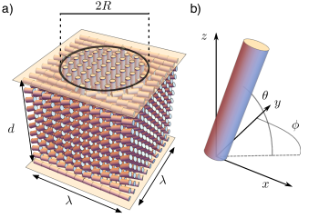
Figure 3: (a) Schematic of the unit cell domain with important length scales labeled for a circle-patterned surface ($a=b=R$ and $\omega=0$). (b) Definition of the polar angle $\theta$ and the azimuthal angle $\phi$ of the LC director.

III.1 Solution

Following previous work, we make the two-constant approximation by setting $K_{1}=K_{3}$ and $K_{2}/K_{1}=\tau$ (Atherton and Sambles, 2006). Additionally, if the polar angle depends on all of the coordinates $\theta=\theta(x,y,z)$ and the azimuthal angle is constant in space $\phi=\phi_{0}$ (Anquetil-Deck et al., 2013), the bulk free energy may be rewritten as a quadratic form,

$$F=\frac{K_{1}}{2}\int\left(\nabla\theta\right)^{T}\cdot A\cdot(\nabla\theta)d^{3}x+\frac{K_{1}}{2L_{\theta}\lambda}\underset{S}{\int}dS\,(\left.\theta\right|_{z=\pm d/2}-\theta_{e})^{2}$$ (4)

where

$$A=\left(\begin{array}[]{ccc}\frac{1}{2}(\alpha-\beta\cos 2\phi_{0})&\frac{1}{2}\beta\sin 2\phi_{0}&0\\ \frac{1}{2}\beta\sin 2\phi_{0}&\frac{1}{2}(\alpha+\beta\cos 2\phi_{0})&0\\ 0&0&1\end{array}\right)$$

and we introduced the dimensionless polar anchoring parameter

$$L_{\theta}=\frac{K_{1}}{W_{\theta}\lambda}.$$ (5)

Within this approximation, minimization of the free energy yields an anisotropic Laplace equation,

$$\mathbf{\nabla}^{T}\cdot A\cdot\mathbf{\nabla}\theta(x,y,z)=0,$$ (6)

where $\alpha\equiv 1+\tau$ and $\beta\equiv 1-\tau$ . This may be solved using the series,

$$\theta(x,y,z)=\overset{\infty}{\!\!\underset{n,m=-\infty}{\sum}\!\!}2A_{nm}\cosh(r_{nm}z)e^{i2\pi(nx+my)},$$ (7)

where

$$\frac{r_{nm}}{\sqrt{2}\pi}=\sqrt{\alpha(m^{2}+n^{2})+\beta(m^{2}-n^{2})\cos 2\phi_{0}+2\beta nm\sin 2\phi_{0}}.$$ (8)

In order to satisfy the boundary conditions, the patterned easy axis is first expanded in a Fourier series,

$$\theta_{e}(x,y)=\overset{\infty}{\underset{n,m=0}{\sum}}S_{nm}e^{i2\pi(nx+my)}.$$ (9)

To determine the coefficients $S_{nm}$, we assume that the background surface promotes $\theta_{e}=0$ while the elliptical pattern promotes $\theta_{e}=\pi/2$, henceforth referred to as “vertical on planar” patterning; the alternative “planar on vertical” arrangement is trivially obtained from this solution by making the substitution,

$$\theta\to\pi/2-\theta,$$ (10)

which leaves the energy invariant. The $S_{nm}$ are therefore evaluated by integrating,

$$S_{nm}=\frac{\pi}{2}\iint_{\mathcal{D}}\exp\big{(}2\pi i(nx+my)\big{)}dxdy,$$ (11)

over a domain $\mathcal{D}$ defined by the ellipse equation,

$$\left(\vec{x}-\vec{x}_{c}\right)^{T}R(\omega)\left(\begin{array}[]{cc}1/a^{2}&0\\ 0&1/b^{2}\end{array}\right)R(-\omega)\left(\vec{x}-\vec{x}_{c}\right)\leq 1.$$ (12)

Here, $R(\omega)$ is the 2D rotation matrix and $\vec{x_{c}}=(\frac{1}{2},\frac{1}{2})$ is the center of the ellipse. As shown in the appendix, the integral (11) can be performed analytically to yield,

$$S_{nm}=\frac{ab\pi}{2}(-1)^{n+m}\frac{J_{1}\left(2\pi\sqrt{a_{nm}^{{}^{\prime}2}+b_{nm}^{{}^{\prime}2}}\right)}{\sqrt{a_{nm}^{{}^{\prime}2}+b_{nm}^{{}^{\prime}2}}},$$ (13)

where $J_{1}(x)$ is a Bessel function of the first kind, $a_{nm}^{{}^{\prime}}=(n\cos\omega+m\sin\omega)a$, and $b_{nm}^{{}^{\prime}}=(n\sin\omega-m\cos\omega)b$.

Having expanded the easy axis in a suitable form, the coefficients $A_{nm}$ can be determined by imposing the Robin boundary condition at $\pm d/2$.

$$\theta_{e}=\left[\pm L_{\theta}\frac{\partial\theta}{\partial z}+\theta\right]_{z=\pm d/2},$$ (14)

Here, the $\pm$ refers to the direction of the outward normal to the LC boundary. Inserting Eqs. (7) and (9) into (14), we obtain,

$$A_{nm}=\frac{S_{nm}}{2\left(L_{\theta}r_{nm}\sinh\left(\frac{r_{nm}d}{2}\right)+\sinh\left(\frac{r_{nm}d}{2}\right)\right)}.$$ (15)

Note that as $L_{\theta}\to 0$, this recovers the rigid anchoring condition. The solution for $\theta(x,y,z)$ is now obtained by inserting Eqs. (15), (13), and (8) into Eq. (7).

As for other patterns (Anquetil-Deck et al., 2012, 2013), the director follows the surface pattern at $\pm d/2$, while relaxing to a uniform orientation, equal to the average polar angle promoted by the surface far away from the boundaries.

III.2 Circular patterns

For a circular surface pattern, set $a=b$ in Eq. (13). Evaluation of the volume integral in Eq. (2) then yields an expression for the bulk energy of the LC,

$$F_{b}=\overset{\infty}{\underset{n,m=-\infty}{\sum}}2K_{1}A_{nm}^{2}\left[B^{T}A\left(\frac{d}{2}\,\textnormal{diag}(1,1,-1)+\frac{\sinh\left(r_{nm}d\right)}{2r_{nm}}I_{3}\right)B\right]$$ (16)

where

$$B=\left(\begin{array}[]{c}2\pi n\\ 2\pi m\\ r_{nm}\end{array}\right).$$

Similarly, evaluation of the surface integral over the surfaces at $+d/2$ and $-d/2$ gives the surface energy of the LC,

$$F_{s}=\overset{\infty}{\underset{n,m=-\infty}{\sum}}\frac{K_{1}\left(S_{nm}-2A_{nm}\cosh(\frac{r_{nm}d}{2})\right)^{2}}{L_{\theta}}.$$

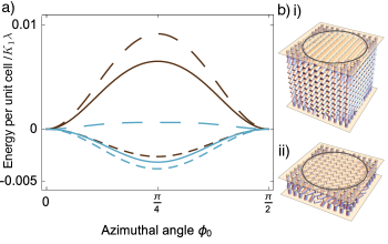
Figure 4: (a) LC surface energy (dotted), bulk energy (dashed), and total energy (solid) as a function of the azimuthal angle for a unit cell of thickness $d/\lambda=1.0$ (brown) and $d/\lambda=0.25$ (cyan) for planar on vertical patterning, $r/\lambda=0.5$, and $L=0.01$. For the thicker unit cell, the surface energy azimuthal preference is much weaker than that of the bulk and the overall preference aligns with that of the bulk. However, thinner cells exhibit weaker bulk energy preference and the total energy favors alignment along $\phi_{0}=\pi/4$. (b) Corresponding calculated structures for i) $d/\lambda=1.0$ and ii) $d/\lambda=0.25$.

The bulk and surface energy of the LC are shown in Fig. 4 as a function of the azimuthal angle $\phi$ for fixed circle radius and polar anchoring energy. The bulk energy always prefers alignment along the $x$- or $y$-axis, but with decreasing strength as the unit cell thickness decreases. Meanwhile, the surface energy prefers director alignment at a 45-degree angle to the axes. This surface preference grows slightly stronger as cell thickness decreases. Results for planar on vertical patterning are identical due to the invariance of the energy under the linear transformation (10).

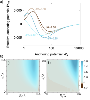
Figure 5: (a) Effective anchoring energy as a function of polar anchoring energy $W_{\theta}$ for $R/\lambda=0.5$ and several cell depths. As the cell depth decreases, the surface preference becomes more pronounced for a given value of $W_{\theta}$. (b) Phase diagram showing the strength and orientation of the preferred azimuthal alignment angle as a function of cell depth $d/\lambda$ and circle radius $R/\lambda$ for i) $L_{\theta}=0.10$0, and ii) $L_{\theta}=0.001$. Brown regions indicate diagonal alignment $\phi_{0}=\pi/4$ while cyan regions regions prefer alignment with the lattice vectors, $\phi_{0}=0$ or $\phi_{0}=\pi/2$. The brown regions expands into larger cell depths as the anchoring strength increases.

We estimate $W_{eff}$, the effective azimuthal surface anchoring energy (Harnau et al., 2007) as the energy difference between the $\phi_{0}=\pi/4$ and the $\phi_{0}=0$ states per unit area. A positive value of $W_{eff}$ indicates a preference for alignment along the $x$- or $y$-axis, while a negative value of $W_{eff}$ indicates a preference for diagonal alignment. Fig. 5(a) shows the effective surface anchoring potential as a function of $W_{\theta}$, the polar anchoring energy, for a series of cell thicknesses. The surface contribution dominates for a thin cell with strong anchoring $W_{\theta}\approx 100$, which corresponds to $L_{\theta}=0.01$. In the limit of rigid anchoring ($W_{\theta}\rightarrow\infty$) or extremely weak anchoring ($W_{\theta}\rightarrow 0$), the effective anchoring vanishes. For weak anchoring, the nematic effectively ignores the pattern, while for rigid anchoring the surface follows the prescribed pattern exactly.

To determine the parameter space in which parallel and diagonal alignment are each favored, we display in Fig. 5(b) the strength of the azimuthal energy preference computed from the combined bulk and surface energies, shown for $L_{\theta}=0.100$, and $L_{\theta}=0.001$. The diagrams indicate two regions in which the the surface preference overrides the bulk preference for a sufficiently thin cell. The strongest of these regions is the thin brown section at $R/\lambda=0.5$, the largest possible circle radius. This region of parameter space is dominated by the surface term, likely due to the inability of vertically/horizontally aligned LCs to effectively fill space between two abutting circles whose edges are nearly perpendicular to the LC director. For circles much smaller than $R=0.5$, the preference becomes very weak indeed.

The comparable magnitude and conflicting preferences of the bulk and surface energies at these length scales suggests that the constant-$\phi$ approximation may be too restrictive for this system. Unlike the rectangular and square patterns previously considered, the alignment direction is promoted exclusively by the lattice while the basis favors no particular alignment. The results of the Monte Carlo simulations also suggest this: in the configurations shown in Fig. 1(b), the particles tend to align tangentially around the edge of the circle because for $\tau<1$ the energetically cheapest way to achieve the vertical-to-planar transition around the perimeter of the circle is through a twist deformation. In section III.4, therefore, we numerically minimize the free energy (2) with respect to a completely arbitrary director profile to quantify the effect of azimuthal variations.

III.3 Elliptical patterns

We now consider elliptical patterns. For long ellipses, one might expect the effective azimuthal alignment to lie parallel to the semi-major axis, resembling the situation with alignment on striped surfaces(Atherton and Sambles, 2006). Hence, by adjusting $\phi$, it should be possible to control the preferred azimuthal angle arbitrarily and, by tuning the aspect ratio, also control the effective azimuthal anchoring energy. The control parameter space to consider is greatly expanded: while the cell depth $d/\lambda$ and the anchoring potential $W_{\theta}$ remain parameters, the circle radius $R/\lambda$ is replaced by the semi major axis length $b/\lambda$, aspect ratio $b/a$, and the alignment angle $\omega$. From the structure of the solution (7), we expect the cell depth and anchoring potential to have similar effects in both patterns and so we focus on the effects of the new parameters in this section.

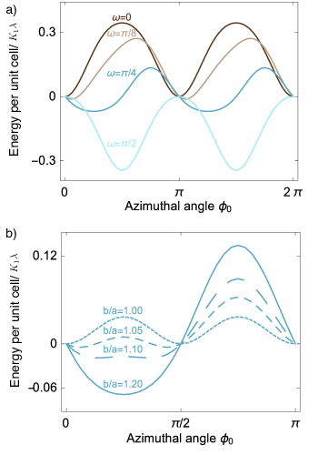
Figure 6: Total LC energy as a function of the azimuthal angle shown for (a) several ellipse rotation angles with $b/a=1.2$ and (b) for several different aspect ratios with $\omega=\pi/4$. Both panels have $d/\lambda=1$, $L_{\theta}=0.01$, and a coverage fraction equal to that of a circle with $R/\lambda=0.4$. Rotation of the ellipse results in migration of the preferred azimuthal angle from alignment with the axes of the unit cell to alignment with the semi major axis of the ellipse. However, panel (b) shows that this transition in azimuthal angle preference is not immediate, but instead passes through several smaller angles as aspect ratio increases.

In Fig. 6, we show effective azimuthal anchoring profiles $W_{eff}(\phi)$ calculated for a variety of values of $\omega$ and $b/a$. The coverage fraction of the pattern, or equivalently the area of the elliptical motif, is kept constant in order to fix the effective polar angle. An immediately obvious feature, compared to the equivalent profiles for circular patterns plotted in Fig. 4, is that the mirror symmetry of the pattern about $\phi=\pi/2$ is entirely broken, leaving behind a non-symmetric anchoring potential reminiscent of the structures fabricated in (Ferjani et al., 2010).

For fairly modest aspect ratios, the alignment angle of the ellipse controls the preferred azimuthal angle such that the energy minima occur at $\phi_{0}=\omega$. For smaller values of $\omega$, or aspect ratios close to unity, the results are more complex: For instance, the energy minimum for $\omega=\pi/8$ in Fig. 6(a) occurs at $\phi_{0}=\pi/16$ instead of $\phi_{0}=\pi/8$. Also, in Fig. 6(b) we see that, for a rotation angle of $\pi/4$, the azimuthal preference moves from alignment with the sides of the unit cell to alignment with the semi major axis of the ellipse gradually, preferring $\phi_{0}=\pi/16$ for an aspect ratio of 1.05 and $\phi_{0}=\pi/8$ for an aspect ratio of 1.1.

The mechanism for this transition is two-fold. Firstly, the surface energy consistently prefers azimuthal alignment along the semi-major axis of the ellipse. Though the angle preferred by the surface remains the same for any non-unit aspect ratio, the strength of the preference grows with increasing aspect ratio. Second, as the aspect ratio grows, the bulk energy of the LC tends to prefer an azimuthal angle aligned with the ellipse alignment angle, but this move happens slowly such that small-to-moderate aspect ratios result in a preferred angle somewhere between $\phi_{0}=0$ and $\phi_{0}=\omega$. The magnitude of the bulk energy preference also grows with increasing aspect ratio, but less dramatically than that of the surface energy preference.

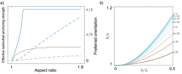
Figure 7: (a) Magnitude (dashed, left axis) and direction (solid, right axis) of azimuthal angle preference given a growing aspect ratio for ellipse alignment angles of $\omega=\pi/4$ (cyan) and $\omega=\pi/8$ (brown) with $d/\lambda=1$, $L_{\theta}=0.01$, and a coverage fraction equal to that of a circle with $R/\lambda=0.4$. (b) Phase diagram of azimuthal angle preference of the entire unit cell as a function of aspect ratio $b/a$ and semi major axis length $b/\lambda$ with $\omega=\pi/4$, $d/\lambda=1$, and $L_{\theta}=0.01$. Note these parameters do not maintain a constant coverage fraction.

The preferred angle $\phi_{0}$ is therefore the result of a tension between surface and bulk effects. We display the direction and strength of the effective anchoring potential as a function of aspect ratio in Fig. 7(a). Fig. 7(b) presents a phase diagram for preferred angle as a function of the semi-major axis and aspect ratio of the elliptical motifs while holding ellipse rotation angle, cell depth, and anchoring potential constant. As expected, increasing aspect ratio leads to alignment of the effective easy axis with the ellipse long axis. Less intuitive is the fact that smaller ellipses transition from alignment with the lattice to alignment with the basis at lower aspect ratios. The decreased scale of the bulk LC energy for small surface features drives this as unit cells with small motifs have surface and bulk energies at the same scale. Thus, increases in aspect ratio quickly shift the LC azimuthal preference to align with the basis, overcoming the influence of the bulk.

III.4 Numerical model

As briefly discussed earlier, the Monte Carlo simulations produced configurations in which the particles tended to align tangentially with the boundary of the circle pattern. These are shown in Fig. 8 and, together with the results of the previous sections, suggest that the constant $\phi$ approximation may be too restrictive for this system. We therefore performed a numerical minimization of the Frank energy (2) again using the two-constant approximation but now allowing the director to vary arbitrarily in 3D. A Cartesian representation of the director $\hat{n}=(n_{x},n_{y},n_{z})$ was used and the unit length constraint $\hat{n}\cdot\hat{n}=1$ enforced locally. The energy was discretized using second-order finite differences and minimized using an adaptive gradient-descent relaxation method with line searches. To improve convergence, successive refinement was used: an initial guess is relaxed on a coarse grid, then interpolated and relaxed onto successively finer grids. At each step, the system was relaxed until the energy converged.

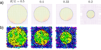
Figure 8: (a) Results from 3D director minimization model. Shown is the director orientation on the bottom face of the unit cell for planar circle patterns of radius $R/\lambda=0.5$, $R/\lambda=0.4$, $R/\lambda=0.33$, and $R/\lambda=0.2$. These simulations are performed with $L_{\theta}=.001$, $d=1.0$, a final grid size of $20\times 20\times 21$, and an initial guess that had the director aligned along the $y$-axis. (b) Corresponding results from Monte Carlo simulations.

Results from the relaxation model for a set of planar patterned surfaces are shown in Fig. 8(a). An initial guess with the director aligned along the $y$-axis was used. After relaxation, the director adopts an orientation tangent to the pattern edges, as seen in the corresponding Monte Carlo simulations, Fig. 8(b). The tangential alignment arises because it corresponds to a twist deformation across the vertical planar boundary, which is energetically cheaper than a bend or splay deformation. The behavior breaks down for smaller circle radii because the bend deformation required to follow the arc of the feature becomes too energetically expensive.

IV Conclusion

This paper has considered the alignment behavior of square arrays decorated with elliptical motifs, demonstrating that such patterns can be used to create surfaces with controllable anchoring energy and easy axis by varying the period of the pattern, ellipse orientation, aspect ratio, and coverage fraction. Given the two-constant approximation and the assumption of a constant azimuthal angle, the director configuration and energy can be computed analytically. Depending on the circle radius, cell depth, and polar anchoring strength of the alignment material, the ground state may have azimuthal alignment along either of the lattice vectors, or diagonally.

Our study offers invaluable advice for applications because, while the elliptical patterned surface offers a remarkable degree of control over the anchoring properties, the design parameter space for the pattern is large. Briefly, surfaces patterned by rotated ellipses allow control of the azimuthal angle over a continuum of values between the lattice vectors and the diagonal depending on the orientation of the ellipse. In these cases, the ellipse aspect ratio controls the effective anchoring energy. The behavior is nontrivial, however, and includes regions of bistability, as well as an azimuthal anchoring transition for some designs.

Unlike for other patterned surfaces previously studied, the constant azimuthal angle approximation is of only limited use. A numerical study showed a preference for tangential alignment along the vertical-planar boundary of the pattern in excellent agreement with Monte Carlo simulations.

While the present study has considered a flat surface, the results may also be important for experimentalists using arrays of posts to align liquid crystals as has been reported in (Kitson and Geisow, 2002; Cavallaro et al., 2013; Lohr et al., 2014). It seems that only a very modest amount of anisotropy in the shape of the pillars, for example using posts of elliptical cross section, may break the square symmetry and lead to significantly better azimuthal alignment if desired.

Appendix

To evaluate the Fourier coefficients for the easy axis, first substitute $x\rightarrow x^{\prime}+1/2$ and $y\rightarrow y^{\prime}+1/2$, which allows (11) and (12) to be rewritten as

$$S_{nm}=\frac{\pi}{2}\exp\big{(}\pi i(n+m)\big{)}\iint_{\mathcal{D}}\exp\big{(}2\pi i(nx^{\prime}+my^{\prime})\big{)}dx^{\prime}dy^{\prime},$$ (17)

and

$$\left(\frac{x^{\prime}\cos\omega+y^{\prime}\sin\omega}{a}\right)^{2}+\left(\frac{x^{\prime}\sin\omega-y^{\prime}\cos\omega}{b}\right)^{2}\leq 1,$$ (18)

respectively. Note that the exponential pre-factor in (17) is $(-1)^{n+m}$ since $n$ and $m$ are integers.

Next, rotate the coordinates via the transformations $(x^{\prime}\cos\omega+y^{\prime}\sin\omega)/a\rightarrow x^{\prime\prime}$ and $(x^{\prime}\sin\omega-y^{\prime}\cos\omega)/b\rightarrow y^{\prime\prime}$, and integrate using these new coordinates,

$$\underset{{}^{(x^{\prime\prime})^{2}+(y^{\prime\prime})^{2}\leq 1}}{S_{nm}=\frac{ab\pi}{2}(-1)^{n+m}\iint\exp\Big{(}2\pi i\big{(}(n\cos\omega+}m\sin\omega)ax^{\prime\prime}+(n\sin\omega-m\cos\omega)by^{\prime\prime}\big{)}\Big{)}dx^{\prime\prime}dy^{\prime\prime}.$$ (19)

Define $a^{\prime}=(n\cos\omega+m\sin\omega)a$, $b^{\prime}=(n\sin\omega-m\cos\omega)b$, $\alpha=(a^{\prime},b^{\prime})$, and $g(s)=\exp(is)$ and convert to polar coordinates such that $(x^{\prime\prime},y^{\prime\prime})\rightarrow r\xi$ where $\xi=(\cos\theta,\sin\theta)$:

$$S_{nm}=\frac{ab\pi}{2}(-1)^{n+m}\int_{0}^{1}r\,dr\int_{\xi}g(2\pi r\alpha\cdot\xi)d\xi.$$ (20)

Eqs. (1.2) and (1.5) from (John, 2004) allow us to evaluate the inner integral to find

$$S_{nm}=\frac{ab\pi}{2}(-1)^{n+m}\int_{0}^{1}2\pi rJ_{0}\left(2\pi r\sqrt{a^{\prime 2}+b^{\prime 2}}\right)dr.$$ (21)

Finally, let $k=2\pi\sqrt{a^{\prime 2}+b^{\prime 2}}$ and $s=kr$, and note that $\int xJ_{0}(x)dx=xJ_{1}(x)$ to obtain,

$$S_{nm} = \frac{ab\pi}{2}(-1)^{n+m}\frac{2\pi}{k^{2}}\int_{0}^{k}sJ_{0}(s)ds$$ (22)

$$= \frac{ab\pi}{2}(-1)^{n+m}\frac{2\pi}{k}J_{1}(k)$$

$$= \frac{ab\pi}{2}(-1)^{n+m}\frac{J_{1}\left(2\pi\sqrt{a^{\prime 2}+b^{\prime 2}}\right)}{\sqrt{a^{\prime 2}+b^{\prime 2}}},$$

the result stated in Eq. (13).

References

- Jerome (1991) B. Jerome, Rep. Prog. Phys. 54, 391 (1991).
- Spencer and Care (2006) T. J. Spencer and C. M. Care, Phys. Rev. E 74, 061708 (2006).
- Kondrat et al. (2003) S. Kondrat, A. Poniewierski, and L. Harnau, The European Physical Journal E 10, 163 (2003).
- Barbero et al. (1992) G. Barbero, T. Beica, A. L. Alexe-Ionescu, and R. Moldovan, Journal de Physique II 2, 2011 (1992).
- Anquetil-Deck et al. (2012) C. Anquetil-Deck, D. J. Cleaver, and T. J. Atherton, Phys. Rev. E 86, 041707 (2012).
- Kim et al. (2001) J. H. Kim, M. Yoneya, J. Yamamoto, and H. Yokoyama, Appl. Phys. Lett. 78, 3055 (2001).
- Yi et al. (2008) Y. W. Yi, V. Khire, C. N. Bowman, J. E. MacLennan, and N. A. Clark, J. Appl. Phys. 103, 1 (2008).
- Yoneya et al. (2002) M. Yoneya, J. H. Kim, and H. Yokoyama, Appl. Phys. Lett. 80, 374 (2002).
- Lee and Clark (2001) B. Lee and N. A. Clark, Science 291, 2576 (2001).
- Kim et al. (2002) J.-H. Kim, M. Yoneya, and H. Yokoyama, Nature 420, 159 (2002).
- Stalder and Schadt (2003) M. Stalder and M. Schadt, Liq. Cryst. 30, 285 (2003).
- Bryan-Brown (2000) G. P. Bryan-Brown, Displays 27, 37 (2000).
- Kitson and Geisow (2002) S. Kitson and A. Geisow, Appl. Phys. Lett. 80, 3635 (2002).
- Hwang and Rey (2006) D. K. Hwang and A. D. Rey, Soc. Ind. Appl. Math. 67, 214 (2006).
- Lowe et al. (2010) A. M. Lowe, B. H. Ozer, Y. Bai, P. J. Bertics, and N. L. Abbott, ACS Appl. Mater. Interfaces 2, 722 (2010).
- Ruan et al. (2003) L. Z. Ruan, J. R. Sambles, and I. W. Stewart, Phys. Rev. Lett. 91, 033901 (2003).
- Wei et al. (2009) L. Wei, J. Weirich, T. T. Alkeskjold, and A. Bjarklev, Opt. Lett. 34, 3818 (2009).
- Bechtold and Oliveira (2005) I. H. Bechtold and E. A. Oliveira, Mol. Cryst. Liq. Cryst. 442, 41 (2005).
- Varghese et al. (2004) S. Varghese, S. Narayanankutty, C. W. M. Bastiaansen, G. P. Crawford, and D. J. Broer, Advanced Materials 16, 1600 (2004).
- Schadt et al. (1992) M. Schadt, K. Schmitt, V. Kozinkov, and V. Chigrinov, Japanese Journal of Applied Physics 31, 2155 (1992).
- Lee et al. (2004) F. K. Lee, B. Zhang, P. Sheng, H. S. Kwok, and O. K. C. Tsui, Appl. Phys. Lett. 85, 5556 (2004).
- Gupta and Abbott (1997) V. K. Gupta and N. L. Abbott, Science 276, 1533 (1997).
- Cheng et al. (2000) Y. L. Cheng, D. N. Batchelder, S. D. Evans, J. R. Henderson, J. E. Lydon, and S. D. Ogier, Liq. Cryst. 27, 1267 (2000).
- Prompinit et al. (2010) P. Prompinit, A. S. Achalkumar, J. P. Bramble, R. J. Bushby, C. Wälti, and S. D. Evans, ACS Appl. Mater. Interfaces 2, 3686 (2010).
- Zheng et al. (2013) W. Zheng, C.-Y. Chiang, and I. Underwood, Thin Solid Films 545, 371 (2013).
- Liu et al. (2012) D. Liu, C. W. M. Bastiaansen, J. M. J. den Toonder, and D. J. Broer, Macromolecules 45, 8005 (2012).
- Park and Park (2008) M. J. Park and O. O. Park, Microelectron. Eng. 85, 2261 (2008).
- Wilderbeek et al. (2003) H. T. A. Wilderbeek, J. P. Teunissen, C. W. M. Bastiaansen, and D. J. Broer, Advanced Materials 15, 985 (2003).
- Atherton and Sambles (2006) T. J. Atherton and J. Sambles, Phys. Rev. E 74, 022701 (2006).
- Atherton et al. (2009) T. J. Atherton, J. R. Sambles, J. P. Bramble, J. R. Henderson, and S. D. Evans, Liq. Cryst. 36, 353 (2009).
- Atherton (2010) T. Atherton, Liq. Cryst. 37, 1225 (2010).
- Ledney and Tarnavskyy (2011) M. Ledney and O. Tarnavskyy, Soft Matter 56, 880 (2011).
- Kondrat et al. (2005) S. Kondrat, A. Poniewierski, and L. Harnau, Liq. Cryst. 32, 95 (2005).
- Yi and Clark (2013) Y. Yi and N. A. Clark, Liq. Cryst. 40, 1736 (2013).
- Anquetil-Deck et al. (2013) C. Anquetil-Deck, D. J. Cleaver, J. P. Bramble, and T. J. Atherton, Phys. Rev. E 88, 012501 (2013).
- Harnau et al. (2007) L. Harnau, S. Kondrat, and A. Poniewierski, Phys. Rev. E 76, 051701 (2007).
- Ferjani et al. (2010) S. Ferjani, Y. Choi, J. Pendery, R. Petschek, and C. Rosenblatt, Phys. Rev. Lett. 104 (2010).
- Cavallaro et al. (2013) M. Cavallaro, M. A. Gharbi, D. A. Beller, S. Čopar, Z. Shi, T. Baumgart, S. Yang, R. D. Kamien, and K. J. Stebe, PNAS 110, 18804 (2013).
- Lohr et al. (2014) M. A. Lohr, M. Cavallaro, D. A. Beller, K. J. Stebe, R. D. Kamien, P. J. Collings, and A. G. Yodh, Soft Matter 10, 3477 (2014).
- John (2004) F. John, Plane waves and spherical means applied to partial differential equations (Dover Publications, 2004).