A noise-induced mechanism for biological homochirality of early life self-replicators

Abstract

The observed single-handedness of biological amino acids and sugars has long been attributed to autocatalysis. However, the stability of homochiral states in deterministic autocatalytic systems relies on cross inhibition of the two chiral states, an unlikely scenario for early life self-replicators. Here, we present a theory for a stochastic individual-level model of autocatalysis due to early life self-replicators. Without chiral inhibition, the racemic state is the global attractor of the deterministic dynamics, but intrinsic multiplicative noise stabilizes the homochiral states, in both well-mixed and spatially-extended systems. We conclude that autocatalysis is a viable mechanism for homochirality, without imposing additional nonlinearities such as chiral inhibition.

One of the very few universal features of biology is homochirality: every naturally occurring amino acid is left-handed (l-chiral) while every sugar is right-handed (d-chiral) Blackmond (2010); Gleiser and Walker (2012). Although such unexpected broken symmetries are well-known in physics, for example in the weak interaction, complete biological homochirality still defies explanation. In 1953, Charles Frank suggested that homochirality could be a consequence of chemical autocatalysis Frank (1953), frequently presumed to be the mechanism associated with the emergence of early life self-replicators. Frank introduced a model in which the d and l enantiomers of a chiral molecule are autocatalytically produced from an achiral molecule $A$ in reactions $A+\textsc{d}\rightarrow 2\textsc{d}$ and $A+\textsc{l}\rightarrow 2\textsc{l}$, and are consumed in a chiral inhibition reaction, $\textsc{d}+\textsc{l}\rightarrow 2A$ . The state of this system can be described by the chiral order parameter $\omega$ defined as $\omega\equiv(d-l)/(d+l)$, where $d$ and $l$ are the concentrations of d and l. The order parameter $\omega$ is zero at the racemic state, and $\pm 1$ at the homochiral states. Frank’s model has three deterministic fixed points of the dynamics; the racemic state is an unstable fixed point, and the two homochiral states are stable fixed points. Starting from almost everywhere in the d-l plane, the system converges to one of the homochiral fixed points (Fig. 1(a)).

In the context of biological homochirality, extensions of Frank’s idea have essentially taken two directions. On the one hand, the discovery of a synthetic chemical system of amino alcohols that amplifies an initial excess of one of the chiral states Soai et al. (1995) has motivated several autocatalysis-based models (see Saito and Hyuga (2013) and references therein). On the other hand, ribozyme-driven catalyst experiments Joyce et al. (1984), have inspired theories based on polymerization and chiral inhibition that minimize Sandars (2003); Gleiser and Walker (2008); Gleiser et al. (2012) or do not include at all Plasson et al. (2004); Brandenburg et al. (2007) autocatalysis. In contrast, a recent experimental realization of RNA replication using a novel ribozyme shows such efficient autocatalytic behavior that chiral inhibition does not arise Sczepanski and Joyce (2014). Further extensions accounting for both intrinsic noise Saito and Hyuga (2013); Lente (2010) and diffusion Shibata et al. (2006); Plasson et al. (2006); Hochberg and Zorzano (2006, 2007) build further upon Frank’s work.

Regardless of the specific model details, all these models share the three-fixed-points paradigm of Frank’s model, namely that the time evolution of the chiral order parameter $\omega$ is given by a deterministic equation of the form Saito and Hyuga (2013)

$$\frac{\text{d}{\omega}}{\text{d}{t}}=f(t)\,\omega\left(1-\omega^{2}\right),$$ (1)

where the function $f(t)$ is model-dependent. However, the homochiral states arise from a nonlinearity which is not a property of simple autocatalysis, but, for instance in the original Frank’s model, is due to chiral inhibition (see Fig. 1(b)). The sole exception to the three-fixed-points model in a variation of Frank’s model is the work of Lente Lente (2004), where purely stochastic chiral symmetry breaking occurs, although chiral symmetry breaking is only partial, with $\omega\neq 0$ but $|\omega|<1$.

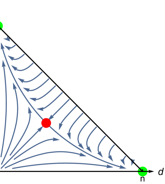
(a) $A+\textsc{d}\rightarrow 2\textsc{d},\hskip 7.22743ptA+\textsc{l}\rightarrow 2\textsc{l},$
     $\textsc{d}+\textsc{l}\rightarrow 2A$

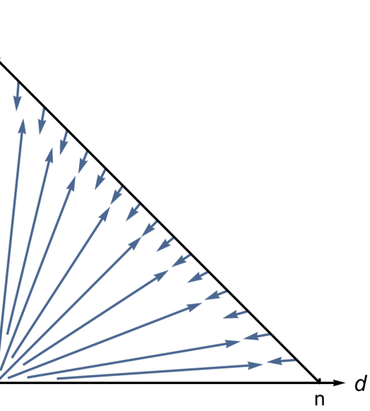
(b) $A+\textsc{d}\rightarrow 2\textsc{d},\hskip 7.22743ptA+\textsc{l}\rightarrow 2\textsc{l},$
     $\textsc{d}\rightarrow A,\hskip 7.22743pt\textsc{l}\rightarrow A$

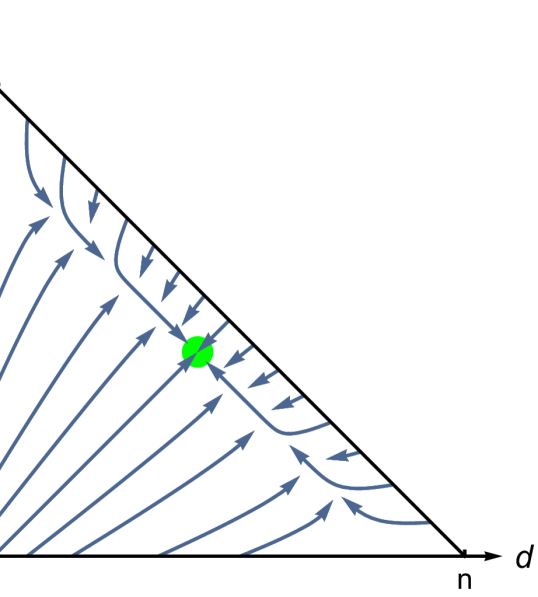
(c) $A+\textsc{d}\rightarrow 2\textsc{d},\hskip 7.22743ptA+\textsc{l}\rightarrow 2\textsc{l},$
     $\textsc{d}\rightleftharpoons A,\hskip 7.22743pt\textsc{l}\rightleftharpoons A$

Figure 1: (Color online) (a) Phase portrait of Frank’s model: the racemic state is an unstable fixed point (red dot), while the homochiral states are stable fixed points (green dots). (b) If chiral inhibition is replaced by linear decay reaction, the ratio of d and l molecules stays constant. (c) Adding even the slightest amount of non-autocatalytic production of d and l molecules makes the racemic state (green dot) the global attractor of the dynamics.

The purpose of this Letter is to show that efficient early-life self-replicators can exhibit universal homochirality, through a stochastic treatment of Frank’s model without requiring nonlinearities such as chiral inhibition. In our stochastic treatment, the homochiral states arise not as fixed points of deterministic dynamics, but instead are states where the effects of chemical number fluctuations (i.e. the multiplicative noise Gardiner (2009)) are minimized. The mathematical mechanism proposed here Togashi and Kaneko (2001); Artyomov et al. (2007); Russell and Blythe (2011); Biancalani et al. (2014) is intrinsically different from that of the class of models summarized by Eq. (1). In the following, we propose a model which we analytically solve for the spatially uniform case and the case of two well-mixed patches coupled by diffusion. We then show, using numerical simulations, that the results persist in a one-dimensional spatially-extended system. We conclude that autocatalysis alone can in principle account for universal homochirality in biological systems.

Stochastic model for well-mixed system:- Motivated in part by the experimental demonstration of autocatalysis without chiral inhibition Sczepanski and Joyce (2014), we propose the reaction scheme below, which is equivalent to a modification of Lente’s reaction scheme Lente (2004) through the additional process representing the recycling of enantiomers:

$$A+\textsc{d}\xrightarrow{\;k_{a}\;}2\textsc{d}, A+\textsc{l}\xrightarrow{\;k_{a}\;}2\textsc{l},$$

$$A\xrightleftharpoons[k_{d}]{\,k_{n}\,}\textsc{d}, A\xrightleftharpoons[k_{d}]{\,k_{n}\,}\textsc{l}.$$ (2)

Compared to Frank’s model, the chiral inhibition is replaced by linear decay reactions which model both recycling and non-autocatalytic production. The rate constants are denoted by $k$, with the subscript serving to identify the particular reaction. The only deterministic fixed point of this model is the racemic state (Fig. 1(c)). This model can be interpreted as a model of the evolution of early life where primitive chiral self-replicators can be produced randomly through non-autocatalytic processes at very low rates; the self-replication is modeled by autocatalysis while the decay reaction is a model for the death process.

We now approximate reaction scheme (2) by means of a stochastic differential equation for the time evolution of the chiral order parameter, $\omega$, which shows that in the regime where autocatalysis is the dominant reaction, the functional form of the multiplicative intrinsic noise from autocatalytic reactions stabilizes the homochiral states. We consider a well-mixed system of volume $V$ and total number of molecules $N$. As shown in the Supplementary Material (SM), for $N\gg 1$, we obtain the following equation for $\omega$, defined in the Itō sense Gardiner (2009):

$$\frac{\text{d}{\omega}}{\text{d}{t}}=-\frac{2k_{n}k_{d}V}{Nk_{a}}\omega+\sqrt{\frac{2k_{d}}{N}(1-\omega^{2})}\eta(t),$$ (3)

where $\eta(t)$ is normalized Gaussian white noise Gardiner (2009).

The time-dependent distribution of Equation (3) can be computed exactly Biancalani et al. (2014, 2015). The stationary distribution Gardiner (2009),

$$P_{s}(\omega)=\mathcal{N}\left(1-\omega^{2}\right)^{\alpha-1},\quad\text{with}\quad\alpha=\frac{Vk_{n}}{k_{a}},$$ (4)

depends on a single parameter, $\alpha$, where the normalization constant $\mathcal{N}$ is given by

$$\mathcal{N}=\left(\int_{-1}^{+1}\left(1-\omega^{2}\right)^{\alpha-1}d\omega\right)^{-1}=\frac{\Gamma\left(\alpha+\frac{1}{2}\right)}{\sqrt{\pi}\;\Gamma(\alpha)}.$$ (5)

Equation (4) is compared in Fig. 2 against Gillespie simulations Gillespie (1977) of scheme (2). For $\alpha=\alpha_{c}=1$, $\omega$ is uniformly distributed. For $\alpha\gg\alpha_{c}$, where the non-autocatalytic production is the dominant production reaction, $P_{s}(\omega)$ is peaked around the racemic state, $\omega=0$. For $\alpha\ll\alpha_{c}$, where autocatalysis is dominant, $P_{s}(\omega)$ is sharply peaked around the homochiral states, $\omega=\pm 1$. The simulations were performed for $N=1000$, where the analytic theory is expected to be accurate; for smaller values of $N$, the theory is qualitatively correct, but very small quantitative deviations are observable compared to the simulations. For example, for $N\sim 100$, $\alpha_{c}\sim 1.005$.

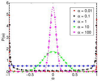
Figure 2: (Color online) Comparison between the stationary distribution, Eq. (4), (dashed lines) and Gillespie simulations of reactions (2) (markers), for different values of $\alpha$. Simulation parameters: $N=10^{3}$, $k_{a}=k_{n}=k_{d}=1$.

The deterministic part of Eq. (3) has one fixed point at the racemic state, consistently with the phase portrait in Fig. 1(c). The multiplicative noise in Eq. (3) vanishes at homochiral states, and admits its maximum at the racemic state. For $\alpha\ll\alpha_{c}$, where autocatalysis is dominant, the amplitude of the noise term in Eq. (3) is much larger than the amplitude of the corresponding deterministic term. In this regime, the system ends up at homochiral states where the noise vanishes.

To understand this result physically, note that the source of the multiplicative noise is the intrinsic stochasticity of the autocatalytic reactions. While, on average, the two autocatalytic reactions do not change the variable $\omega$, each time one of the reactions takes place, the value of $\omega$ changes by a very small discrete amount. As a result, over time the value of $\omega$ drifts away from its initial value. Since the amplitude of the noise term is maximum at racemic state and zero at homochiral states, this drift stops at one of the homochiral states. The absence of the noise from autocatalysis at homochiral states can be understood by recognizing that at homochiral states, the molecules with only one of two chiral states d and l are present, hence only the autocatalytic reaction associated with that chiral state has a non-zero rate. This reaction produces molecules of the same chirality, keeping the system at the same homochiral state without affecting the value of $\omega$, and therefore, the variable $\omega$ does not experience a drift away from the homochiral states due the autocatalytic reactions.

Since the stationary distribution of $\omega$ in Eq. (4) is only dependent on $\alpha$, the decay reaction rate, $k_{d}$ has no effect on the steady state distribution of the system. The only role of this reaction is to prevent the $A$ molecules from being completely consumed, thus providing a well-defined non-equilibrium steady state independent of the initial conditions. The parameter $\alpha$ is proportional to the ratio of the non-autocatalytic production rate, $k_{n}$, to the self-replication rate, $k_{a}$. In the evolution of early life, when self-replication was a primitive function, $k_{a}$ would be small and the value of $\alpha$ would therefore be large; but as self-replication became more efficient, the value of $k_{a}$ would increase and so $\alpha$ would decrease. Therefore, in our model, we expect that life started in a racemic state, and it transitioned to complete homochirality through the mechanism explained above, after self-replication became efficient (i.e. when $\alpha\ll\alpha_{c}$).

It is important to note that all of the previous mechanisms suggested for homochirality rely on assumptions that cannot be easily confirmed to hold during the emergence of life. However, even if all of such mechanisms fail during the origin of life, our mechanism guarantees the emergence of homochirality, since it only relies on self-replication and death, two processes that are inseparable from any living system.

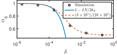
Figure 3: (Color online) Parameter $\alpha_{c}^{\text{patch}}$ in the two-patch system as a function of the diffusion rate $\delta$. Gillespie simulations (markers) are compared against Eq. (11) (solid blue line) and Eq. (13) (dashed red line). Simulation parameters as in Fig. 2.

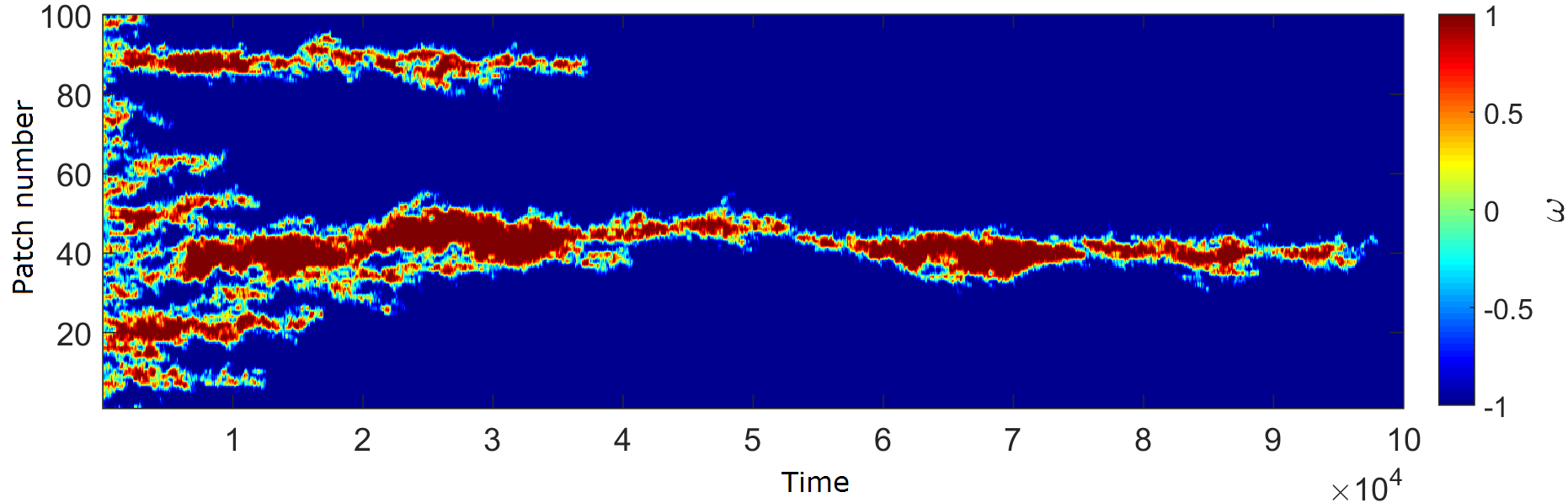
Figure 4: (Color online) Gillespie simulation of scheme (6) for a one-dimensional system of $M=100$ patches, starting from racemic state and ending with all the patches in the same homochiral state $\omega=-1$. Simulation parameters: $N=1000$, $k_{a}=k_{d}=1$, $\delta=10^{-3}$, and $k_{n}=0$.

Stochastic model with spatial extension:- We now turn to the study of reaction scheme (2) generalized to the spatially-extended case McKane and Newman (2004). We discretize space into a collection of $M$ patches of volume $V$, indexed by $i$. The geometry of the space is defined by $\langle i\rangle$ — the set of patches that are nearest-neighbor to patch $i$ (e.g., for a linear chain, $\langle i\rangle=\{i-1,i+1\}$). We indicate the molecules of species $A$ in patch $i$ by $A_{i}$ and similarly for the other species. Each patch is well-mixed and reactions (2) occur within, while molecules can diffuse between neighboring patches with diffusion rate $\delta$. In summary, the following set of reactions defines the spatial model:

$$\begin{split}&A_{i}\xrightleftharpoons[k_{d}]{\,k_{n}\,}\textsc{d}_{i},\quad A_{i}\xrightleftharpoons[k_{d}]{\,k_{n}\,}\textsc{l}_{i},\quad i=1,\ldots,M\\ &A_{i}+\textsc{d}_{i}\xrightarrow{\;k_{a}\;}2\textsc{d}_{i},\quad A_{i}+\textsc{l}_{i}\xrightarrow{\;k_{a}\;}2\textsc{l}_{i}\\ &\textsc{d}_{i}\xrightleftharpoons{\;\delta\;}\textsc{d}_{j},\quad\textsc{l}_{i}\xrightleftharpoons{\;\delta\;}\textsc{l}_{j},\quad j\in\langle i\rangle.\end{split}$$ (6)

We now derive the following set of coupled stochastic differential equation for the time evolution of the chiral order parameter $\omega_{i}$, of each patch $i$ (see SM)

$$\begin{split}\frac{\text{d}{\omega_{i}}}{\text{d}{t}}=&-\frac{2k_{n}k_{d}V}{Nk_{a}}\omega_{i}+\delta\sum_{j\in\langle i\rangle}(\omega_{j}-\omega_{i})\\ &+\sqrt{\frac{2k_{d}}{N}(1-\omega_{i}^{2})}\eta_{i}(t)+\sqrt{\frac{\delta}{N}}\xi_{i}(\vec{\omega},t),\end{split}$$ (7)

where now $N$ represents the average number of molecules per patch, $\eta_{i}$’s are independent normalized Gaussian white noises, $\xi_{i}$’s are zero mean Gaussian noise with correlator

$$\begin{split}\langle\xi_{i}(t)\xi_{j}(t^{\prime}{})\rangle=&\left(2\sum_{k\in\langle i\rangle}\left(1-\omega_{i}\omega_{k}\right)\delta_{i,j}\right.\\ &\;\;\left.+\left(\omega_{i}^{2}+\omega_{j}^{2}-2\right){\mathchoice{\raisebox{0.0pt}{$\displaystyle\chi$}}{\raisebox{0.0pt}{$\textstyle\chi$}}{\raisebox{0.0pt}{$\scriptstyle\chi$}}{\raisebox{0.0pt}{$\scriptscriptstyle\chi$}}}_{\langle i\rangle}(j)\vphantom{\sum_{k\in\langle i\rangle}}\right)\delta(t-t^{\prime}{}),\end{split}$$ (8)

and ${\mathchoice{\raisebox{0.0pt}{$\displaystyle\chi$}}{\raisebox{0.0pt}{$\textstyle\chi$}}{\raisebox{0.0pt}{$\scriptstyle\chi$}}{\raisebox{0.0pt}{$\scriptscriptstyle\chi$}}}_{\langle i\rangle}(j)$ is equal to one if $j\in\langle i\rangle$ and zero otherwise.

In order to see how the coupling of well-mixed patches affects their approach to homochirality, it is instructive to consider the simplest case of two adjacent patches ($M=2$). In the two-patch model, various scenarios can happen: the system may not exhibit homochirality ($\omega_{1}\sim\omega_{2}\sim 0$); each patch can separately reach homochirality ($\omega_{1}=\pm 1$ and $\omega_{2}=\pm 1$); the system exbihits global homochirality ($\omega_{1}=\omega_{2}=\pm 1$). We first analyze the condition for each patch reaching homochirality using perturbation theory, in the case of slow diffusion. The stationary probability density function of the chiral order parameter of a single patch, $Q_{s}(\omega)$ is defined by

$$Q_{s}(\omega)=\int_{-1}^{+1}Q_{s}(\omega,\omega_{2})d\omega_{2}=\int_{-1}^{+1}Q_{s}(\omega_{1},\omega)d\omega_{1},$$ (9)

where $Q_{s}(\omega_{1},\omega_{2})$ is the joint probability distribution of $\omega_{1}$ and $\omega_{2}$ at steady state from Eq. (7). If $\delta\sim k_{d}/N$ or smaller, then (see SM) the stationary distribution reads

$$Q_{s}(\omega)=\mathcal{Z}(1-\omega^{2})^{\alpha+\frac{\delta N}{2k_{d}}-1},$$ (10)

where $\mathcal{Z}$ is a normalization constant. This result shows that the critical $\alpha$ in a single patch, up to the first order correction in $\delta$, is given by

$$\alpha_{c}^{\text{patch}}\approx 1-\delta\frac{N}{2k_{d}},\quad\text{for }\delta\approx 0.$$ (11)

We can now turn to the case of high diffusion. Recall that the patches are defined as the maximum volume around a point in space in which the system can be considered well-mixed. This can be interpreted as the maximum volume in which diffusion dominates over the other terms acting on the variable of interest (in this case $\omega$). From Eq. (7), this condition is fulfilled for $\delta\sim 2k_{d}\alpha/N$. In the vicinity of the transition $\alpha$ is in order of one, therefore the condition becomes $\delta\sim k_{d}/N$. For $\delta\gg k_{d}/N$, the whole system can be considered well-mixed, and we can find the critical value of $\alpha$ for each patch, starting from $\alpha_{c}=1$, from the well-mixed results, and using as volume the volume the whole system, i.e., $MV$. This indicates that in a single patch

$$\alpha_{c}^{\text{patch}}\approx\frac{1}{M},\quad\text{for }\delta\gg 0.$$ (12)

A simple formula that interpolates between these extreme limits, asymptotic to $1/M$ (with $M=2$) for large $\delta$ and to Eq. (11) for small $\delta$, is

$$\alpha_{c}^{\text{patch}}=\frac{\delta+2\delta^{*}}{2\delta+2\delta^{*}},\hskip 14.45377pt\delta^{*}=\frac{k_{d}}{N}.$$ (13)

Figure 3 shows agreement between $\alpha_{c}^{\text{patch}}$ measured from Gillespie simulations of the two-patch system, and the Eq. (13). At the parameter regime below the $\alpha_{c}$ curve in Fig. 3, individual patches are homochiral. Also, we find that the correlation between the homochiral states of the two patches increases with diffusion rate $\delta$ and become completely correlated when $\delta\sim k_{d}/N$ or more. In this regime the system reaches global homochirality.

This latter result suggests that in the spatially-extended model, when autocatalysis is the dominant reaction (i.e. $\alpha$ is small enough) and when the diffusion rate is in the order of $k_{d}/N$ or larger, all patches converge to the same homochiral state. Figure 4 shows the dynamics of a Gillespie simulation of a one-dimensional chain of $100$ patches, initializes at the racemic state, in the pure autocatalytic limit ($k_{n}\to 0$). Very quickly, small islands of different homochirality (blue and red) are formed. Islands of opposite chirality competes against each other, until the system reaches global homochirality. Note that for $\delta\sim k_{d}/N$ we can treat the diffusion process deterministically by ignoring the last term in Eq. (7). In this regime, Eq. (7) is the same as the equation describing one-dimensional voter model, implying that the transition to homochirality is in the universality class of compact directed percolation Dickman and Tretyakov (1995).

In conclusion, a racemic population of self-replicating chiral molecules far from equilibrium, even in the absence of other nonlinearities that have previously been invoked, such as chiral inhibition, transitions to complete homochirality when the efficiency of self-replication exceeds a certain threshold. This transition occurs due to the drift of the chiral order parameter under the influence of the intrinsic stochasticity of the autocatalytic reactions. The functional form of the multiplicative intrinsic noise from autocatalysis directs this drift toward one of the homochiral states. Unlike some other mechanisms in the literature, this process does not require an initial enantiomeric excess. In our model, the homochiral states are not deterministic dynamical fixed points, but are instead stabilized by intrinsic noise. Moreover, in the spatial extension of our model, we have shown that diffusively coupled autocatalytic systems synchronize their final homochiral states, allowing a system solely driven by autocatalysis to reach global homochirality. We conclude that autocatalysis alone is a viable mechanism for homochirality, without the necessity of imposing chiral inhibition or other nonlinearities.

I SUPPLEMENTARY MATERIAL

I.1 Well-Mixed System

We start from reaction scheme (2) of the main paper

$$\begin{split}&A+\textsc{d}\xrightarrow{\;k_{a}\;}2\textsc{d},A+\textsc{l}\xrightarrow{\;k_{a}\;}2\textsc{l},\\ &A\xrightleftharpoons[k_{d}]{\,k_{n}\,}\textsc{d},A\xrightleftharpoons[k_{d}]{\,k_{n}\,}\textsc{l}.\end{split}$$ (S1)

Each reaction changes the system from a state $\vec{x}\equiv(x_{1},x_{2},x_{3})\equiv(a,d,l)$, specified by the concentration of molecules $A$, d, and l, to a state of the form $\vec{x}+V^{-1}\vec{s}_{m}$ (for some $m\in\{1,\ldots,4\}$), where $\vec{s}_{m}$ is the $m$’th row of the stoichiometry matrix

$$\mathbf{S}=\left(\begin{array}[]{ccc}-1&1&0\\ -1&0&1\\ 1&-1&0\\ 1&0&-1\end{array}\right).$$ (S2)

The probability per unit time of such transition is given by transition rates $T(\vec{x}+V^{-1}\vec{s}_{m}|\vec{x})$ obtained from law of mass action for reactions (S1):

$$\begin{split}T(\vec{x}+\frac{1}{V}\vec{s}_{1}|\vec{x})&=V(k_{n}+k_{a}d)a,\quad T(\vec{x}+\frac{1}{V}\vec{s}_{3}|\vec{x})=Vk_{d}d,\\ T(\vec{x}+\frac{1}{V}\vec{s}_{2}|\vec{x})&=V(k_{n}+k_{a}l)a,\quad T(\vec{x}+\frac{1}{V}\vec{s}_{4}|\vec{x})=Vk_{d}l.\end{split}$$ (S3)

The set of rates (S3) is used to write the master equation for the time evolution of the probability density function, $P(\vec{x},t)$, of the system being in the state $\vec{x}$ at time $t$ van Kampen (2007). We begin by defining the functions $F_{m}$’s as

$$F_{m}(\vec{x},t)=T(\vec{x}|\vec{x}-\frac{1}{V}\vec{s}_{m})P(\vec{x}-\frac{1}{V}\vec{s}_{m},t),$$ (S4)

so that the master equation can be written as:

$$\begin{split}\frac{\partial{P(\vec{x},t)}}{\partial{t}}=-\sum_{m=1}^{4}\left(F_{m}(\vec{x}+\frac{1}{V}\vec{s}_{m},t)-F_{m}(\vec{x},t)\right).\end{split}$$ (S5)

This equation defines the stochastic model and can be numerically simulated using the Gillespie algorithm Gillespie (1977).

In order to initiate an analytical treatment, we begin by expanding the right-hand side of the master equation (we follow McKane et al. (2014)). We obtain a Gaussian noise approximation by truncating the expansion at the second-order, thus neglecting terms corresponding to higher moments. We arrive at the non-linear Fokker-Planck equation:

$$\begin{split}\frac{\partial{P}}{\partial{t}}\approx-\sum_{j=1}^{3}\frac{\partial{\left(H_{j}P\right)}}{\partial{x_{j}}}+\frac{1}{2}\sum_{j,k=1}^{3}\frac{\partial^{2}\left(B_{jk}P\right)}{\partial x_{j}\partial x_{k}},\end{split}$$ (S6)

where the drift vector $\vec{H}$ with component $H_{j}$ reads:

$$\begin{split}\vec{H}=&\frac{1}{V}\sum_{m}T(\vec{x}+\frac{1}{V}\vec{s}_{m})|\vec{x})\vec{s}_{m}\\ =&\left(\begin{array}[]{c}k_{d}(d+l)-a(2k_{n}+k_{a}(d+l))\\ -k_{d}d+a(k_{n}+k_{a}d)\\ -k_{d}l+a(k_{n}+k_{a}l)\end{array}\right).\end{split}$$ (S7)

The symmetric diffusion matrix has the form

$$\mathbf{B}=\frac{1}{V^{2}}\sum_{m}T(\vec{x}+\frac{1}{V}\vec{s}_{m})|\vec{x})\left(\vec{s}_{m}\otimes\vec{s}_{m}\right)=\frac{1}{V}\left(\begin{array}[]{ccc}k_{d}(d+l)+a(2k_{n}+k_{a}(d+l))&-k_{d}d-a(k_{n}+k_{a}d)&-k_{d}l-a(k_{n}+k_{a}l)\\ -k_{d}d-a(k_{n}+k_{a}d)&k_{d}d+a(k_{n}+k_{a}d)&0\\ -k_{d}l-a(k_{n}+k_{a}l)&0&k_{d}l+a(k_{n}+k_{a}l)\end{array}\right),$$ (S8)

where the symbol $\otimes$ indicates the Kronecker product. We now decompose the diffusion matrix to $\mathbf{B}=\mathbf{G}\mathbf{G}^{T}$. Multiple choices for $\mathbf{G}$ exist McKane et al. (2014), and it is easy to check that the following $3\times 2$ matrix satisfies the decomposition:

$$\begin{split}\mathbf{G}=\frac{1}{\sqrt{V}}\left(\begin{array}[]{cc}\sqrt{a\left(k_{a}d+k_{n}\right)+k_{d}d}&\sqrt{a(k_{a}l+k_{n})+k_{d}l}\\ -\sqrt{a\left(k_{a}d+k_{n}\right)+k_{d}d}&0\\ 0&-\sqrt{a(k_{a}l+k_{n})+k_{d}l}\end{array}\right).\end{split}$$

Equation (S6) is equivalent to the following stochastic differential equation (defined in the Itō sense) Gardiner (2009)

$$\frac{\text{d}{\vec{x}}}{\text{d}{t}}=\vec{H}(\vec{x})+\mathbf{G}(\vec{x})\vec{\eta}(t)$$ (S10)

where $\eta_{k}$’s ($k=1,2$) are Gaussian white noises with zero mean and correlation

$$\langle\eta_{j}(t)\eta_{k}(t^{\prime})\rangle=\delta_{jk}\delta(t-t^{\prime}).$$ (S11)

Note that since, the Fokker-Planck equation (S6) only depends on $\mathbf{B}$ and not the particular choice of its decomposition $\mathbf{G}$, the probability density function of $\vec{x}$ and its time evolution do not depend on $\mathbf{G}$ either McKane et al. (2014).

The number of degrees of freedom in Eq. (S10) can be reduced by noting two facts: (i) the reaction scheme (S1) conserves the total number of molecules, meaning that the total concentration $n=a+d+l$ is conserved; (ii) simulations show that the concentration $r=d+l$ settles to a Gaussian distribution around its fixed point value $r^{*}$, allowing us to substitute $r(t)\to r^{*}$. We therefore change variables in Eq. (S10) (using Itō’s formula) Gardiner (2009), from

$$\left(\begin{array}[]{c}a\\ d\\ l\end{array}\right)\to\left(\begin{array}[]{c}n\\ r\\ \omega\end{array}\right)=\left(\begin{array}[]{c}a+d+l\\ d+l\\ (d-l)/(d+l)\end{array}\right),$$ (S12)

so that the only dynamics occurs in the chiral order parameter $\omega$. In the new variables, we find that $\dot{n}=0$ and, by taking the positive solution of $\dot{r}=0$, that is

$$r^{*}=\frac{\sqrt{(k_{a}n-k_{d}-2k_{n})^{2}+8k_{a}k_{n}n}+k_{a}n-k_{d}-2k_{n}}{2k_{a}},$$ (S13)

we substitute $r\to r^{*}$ in the equation for $\omega$, and use the rule for summing Gaussian variables (i.e. $a\eta_{1}+b\eta_{2}=\sqrt{a^{2}+b^{2}}\eta$; where $a$ and $b$ are generic functions Gardiner (2009)) to express the stochastic part of the equation using a single noise variable. Expressing the result in terms of the total number of molecules $N=Vn$, for $N\gg 1$, we arrive at the following stochastic differential equation for chirality order parameter $\omega$ (equation (2) of the main text):

$$\frac{\text{d}{\omega}}{\text{d}{t}}=-\frac{2k_{n}k_{d}V}{Nk_{a}}\omega+\sqrt{\frac{2k_{d}}{N}(1-\omega^{2})}\eta(t),$$ (S14)

where $\eta(t)$ is Gaussian white noise with zero mean and unit variance. The corresponding Fokker-Planck equation of Eq. (S14) is an exactly solvable partial differential equation with time dependent solution given in Biancalani et al. (2015). The steady state probability distribution of $\omega$ is given by

$$P_{s}(\omega)=\mathcal{N}\left(1-\omega^{2}\right)^{\alpha-1},\quad\text{with}\quad\alpha=\frac{Vk_{n}}{k_{a}},$$ (S15)

with the normalization constant

$$\mathcal{N}=\left(\int_{-1}^{+1}\left(1-\omega^{2}\right)^{\alpha-1}\text{d}\omega\right)^{-1}=\frac{\Gamma\left(\alpha+\frac{1}{2}\right)}{\sqrt{\pi}\;\Gamma(\alpha)}.$$ (S16)

I.2 Two-patch model

Starting from reaction scheme (6) of the main paper for the spatial extension of our model

$$\begin{split}&A_{i}\xrightleftharpoons[k_{d}]{\,k_{n}\,}\textsc{d}_{i},\quad A_{i}\xrightleftharpoons[k_{d}]{\,k_{n}\,}\textsc{l}_{i},\quad i=1,\ldots,M\\ &A_{i}+\textsc{d}_{i}\xrightarrow{\;k_{a}\;}2\textsc{d}_{i},\quad A_{i}+\textsc{l}_{i}\xrightarrow{\;k_{a}\;}2\textsc{l}_{i}\\ &\textsc{d}_{i}\xrightleftharpoons{\;\delta\;}\textsc{d}_{j},\quad\textsc{l}_{i}\xrightleftharpoons{\;\delta\;}\textsc{l}_{j},\quad j\in\langle i\rangle,\end{split}$$ (S17)

for $M=2$, we can follow the procedure explained in the previous section to obtain a Fokker-Planck equation for time evolution of the probability density of system being at a state with concentrations $a_{1}$, $d_{1}$, $l_{1}$, $a_{2}$, $d_{2}$, and $l_{2}$. Again we can reduce the number of variables using the following facts (i) the total concentration $n_{t}=n_{1}+n_{2}=a_{1}+d_{1}+l_{1}+a_{2}+d_{2}+l_{2}$ is conserved; (ii) simulation shows that in long time, the variables $r_{1}=d_{1}+l_{1}$, $r_{2}=d_{2}+l_{2}$, and $\Delta=n_{1}-n_{2}$ settle to Gaussian distributions around their fixed point values $r_{1}=r_{2}=r^{*}$ and $\Delta=0$. We do the following change of variables

$$\left(\begin{array}[]{c}a_{1}\\ d_{1}\\ l_{1}\\ a_{2}\\ d_{2}\\ l_{2}\end{array}\right)\to\left(\begin{array}[]{c}n_{t}\\ \Delta\\ r_{1}\\ r_{2}\\ \omega_{1}\\ \omega_{2}\end{array}\right)=\left(\begin{array}[]{c}a_{1}+d_{1}+l_{1}+a_{2}+d_{2}+l_{2}\\ a_{1}+d_{1}+l_{1}-a_{2}-d_{2}-l_{2}\\ d_{1}+l_{1}\\ d_{2}+l_{2}\\ (d_{1}-l_{1})/(d_{1}+l_{1})\\ (d_{2}-l_{2})/(d_{2}+l_{2})\end{array}\right)$$ (S18)

using Itō’s formula. Now the dynamics only occurs only in $\vec{\omega}=(\omega_{1},\omega_{2})$. For large average number of molecules per patch $N\gg 1$, the resulting Fokker-Planck equation for time evolution of the joint probability density function of $\omega_{1}$ and $\omega_{2}$, $Q(\vec{\omega},t)$, reads

$$\begin{split}\frac{\partial{Q}}{\partial{t}}=-\sum_{i=1}^{2}\frac{\partial{\left(\left(\mathbf{L}\vec{\omega}\right)_{i}Q\right)}}{\partial{\omega_{i}}}+\frac{1}{2}\sum_{i,j=1}^{2}\frac{\partial^{2}\left(U_{ij}Q\right)}{\partial\omega_{i}\partial\omega_{j}}.\end{split}$$ (S19)

Note that the above sums are now over the patches, and not over species as in Eq. (S6). The Jacobian matrix $\mathbf{L}$

$$\mathbf{L}=-\frac{2k_{d}k_{n}V}{Nk_{a}}\left(\begin{array}[]{cc}1&0\\ 0&1\end{array}\right)+\delta\left(\begin{array}[]{cc}-1&1\\ 1&-1\end{array}\right),$$ (S20)

and the diffusion matrix $\mathbf{U}$ reads

$$\begin{split}\mathbf{U}=&\;\frac{2k_{d}}{N}\left(\begin{array}[]{cc}1-\omega_{1}^{2}&0\\ 0&1-\omega_{2}^{2}\end{array}\right)\\ &+\frac{\delta}{N}\left(\begin{array}[]{cc}2(1-\omega_{1}\omega_{2})&\omega_{1}^{2}+\omega_{2}^{2}-2\\ \omega_{1}^{2}+\omega_{2}^{2}-2&2(1-\omega_{1}\omega_{2}).\end{array}\right).\end{split}$$ (S21)

Note that the stochastic differential equation corresponding to Eq. (S19) is the $M=2$ case of equation (7) of the main paper.

I.3 Perturbation theory for the small diffusion case

Now, we can use perturbation theory for small $\delta$, to find the stationary probability density of $\omega$ for each patch defined as

$$Q_{s}(\omega)=\int_{-1}^{+1}Q_{s}(\omega,\omega_{2})\text{d}\omega_{2}=\int_{-1}^{+1}Q_{s}(\omega_{1},\omega)\text{d}\omega_{1},$$ (S22)

where $Q_{s}(\omega_{1},\omega_{2})$ is the stationary solution of Eq. (S19). For $\delta\sim k_{d}/N$ or smaller, we can treat the diffusion deterministically by ignoring the last term in Eq. (S21). To solve for $Q_{s}(\omega)$, we begin by rewriting Eq. (S19) as a continuity equation,

$$\partial_{t}Q+\nabla\cdot\vec{J}=0,$$ (S23)

which defines the probability current $\vec{J}$ as Gardiner (2009)

$$\vec{J}=\mathbf{L}\vec{\omega}\;Q-\frac{1}{2}\nabla\cdot\left(\mathbf{U}Q\right).$$ (S24)

By the conservation of probability, at stationary conditions, the total probability flux $\vec{J}_{s}$ through each vertical section of $\omega_{1}$-$\omega_{2}$ plane must be zero. That is

$$\begin{split}&\int_{-1}^{+1}J_{s,1}\text{d}\omega_{2}=\int_{-1}^{+1}\left((\mathbf{L}\vec{\omega})_{1}Q_{s}-\frac{1}{2}\partial_{\omega_{1}}(U_{11}Q_{s})\right)\text{d}\omega_{2}\\ &=\;Q_{s}(\omega_{1})\omega_{1}\left(\frac{2k_{d}}{N}(1-\alpha)-\delta\right)-\frac{k_{d}}{N}(1-\omega_{1}^{2})\frac{\text{d}{Q_{s}}}{\text{d}{\omega_{1}}}\\ &+\delta\int_{-1}^{+1}\omega_{2}Q_{s}(\omega_{1},\omega_{2})\text{d}\omega_{2}=0.\end{split}$$ (S25)

The last integral can be evaluated using Bayes’ theorem

$$\begin{split}\delta\int_{-1}^{+1}\omega_{2}&Q_{s}(\omega_{1},\omega_{2})\text{d}\omega_{2}=\delta\int_{-1}^{+1}\omega_{2}Q_{s}(\omega_{2}|\omega_{1})Q_{s}(\omega_{1})\text{d}\omega_{2}\\ &=\delta\;Q_{s}(\omega_{1})\langle\omega_{2}\rangle_{\omega_{1}}=\mathcal{O}(\delta^{2}),\end{split}$$ (S26)

which is of order $\delta^{2}$ for small $\delta$, since, $\langle\omega_{2}\rangle_{\omega_{1}}$ (the expected value of $\omega_{2}$ given $\omega_{1}$) vanishes at zero $\delta$, and therefore, of order $\delta$ for small $\delta$. In this regime, Eq. (S25) provide us with a differential equation for $Q_{s}(\omega)$ with the solution (equation (10) of the main paper)

$$Q_{s}(\omega)=\mathcal{Z}(1-\omega^{2})^{\alpha+\frac{\delta N}{2k_{d}}-1},$$ (S27)

where the normalization constant $\mathcal{Z}$ is given by

$$\mathcal{Z}=\frac{\Gamma\left(\alpha+\frac{\delta N}{2k_{d}}+\frac{1}{2}\right)}{\sqrt{\pi}\;\Gamma(\alpha+\frac{\delta N}{2k_{d}})}.$$ (S28)