Rapid magnetic oscillations and magnetic breakdown in quasi-1D conductors

Abstract

We review the physics of magnetic quantum oscillations in quasi-one dimensional conductors with an open Fermi surface, in the presence of modulated order. We emphasize the difference between situations where a modulation couples states on the same side of the Fermi surface and a modulation couples states on opposite sides of the Fermi surface. We also consider cases where several modulations coexist, which may lead to a complex reorganization of the Fermi surface. The interplay between nesting effects and magnetic breakdown is discussed. The experimental situation is reviewed.

I Introduction

It is well known that magnetic oscillations in thermodynamic and transport properties originate from the Landau quantization of closed electronic orbits. The existence of such oscillations in quasi-1D conductors with an open Fermi Surface (FS), especially studied in compounds of the Bechgaard salts family, has thus been a long standing problem (for a review, see Refs.[Lebedbook, ; Yamajibook, ]). Various mechanisms have been invoked to explain the existence of these quantum oscillations in the presence of open orbits. Most of them are based on the existence of an external periodic potential which permits a modification of the Fermi surface. Other mechanisms like the magnetic field modulation of electron-electron scatteringeescattering and the rich physics of the angular oscillations are not discussed here.Yamajibook

One of these mechanisms is the Density Wave (DW) ordering due to almost perfect nesting of the Fermi surface (FS). Such ordering leaves small closed electronic pockets of unpaired carriers the size of which is related to the deviation from perfect nesting, as recalled later in this paper (Fig. 5). In a magnetic field ${B}$ applied along a direction perpendicular to the most conducting planes, the quantization of the electronic motion along these closed pockets leads to Shubnikov-de Haas (SdH) oscillations (periodic in $1/{B}$) the period of which is proportional to the size of the pocket. The typical field ${B_{f}}$ characteristic of the oscillations is proportional to the area ${\cal A}$ of the closed orbits in reciprocal space ${B_{f}}={\hbar\over 2\pi e}{\cal A}$. The characteristic energy of deviation from perfect nesting, named $t^{\prime}_{b}$, is usually of order of $10$-$30$ K, so that ${\cal A}\propto{t^{\prime}_{b}\over\hbar v_{F}b}$ and the typical field ${B_{f}}\propto{t^{\prime}_{b}\over ev_{F}b}$ is of order of a few dozen teslas. In Bechgaard salts, the competition between Spin Density Wave (SDW) ordering and the quantization due the magnetic field leads to a cascade of SDW subphases in which the Hall effect is quantized.Lebedbook ; Yamajibook ; GL ; FISDW ; Yakovenko

In this paper, we focus our study to the understanding of the so-called Rapid Oscillations (RO), described by a much larger characteristic field, of order of few hundred teslas, believed to be related to the typical warping of the FS related to an energy scale $t_{b}\gg t_{b}^{\prime}$, therefore to much larger orbits the existence of which cannot be explained by DW ordering alone (${\cal A}\propto{t_{b}\over\hbar v_{F}b}$ and ${B_{f}}\propto{t_{b}\over ev_{F}b}$).

We examine various kind of external periodic potentials which may give rise to such rapid oscillations. We consider a simple band model in order to study the effect of different modulations on the electronic spectrum and their consequence on the structure of the magnetic field induced quantum oscillations. We start from the widely used two-dimensional tight-binding model describing a metallic phase with a simple orthorhombic dispersion with hopping parameters $t_{a}$ along the $x$ direction of the conducting chains and $t_{b}$ along the perpendicular $y$ direction. The magnetic field is applied along the $z$ direction (the $c^{*}$ direction in Bechgaard salts having triclinic symmetry). The dispersion relation may be linearized along the high conductivity direction and the modulation along the transverse direction is then described by two harmonics with amplitudes $t_{b}$ and $t^{\prime}_{b}$ :Lebedbook ; Yamajibook ; GL ; FISDW

$$\epsilon_{\boldsymbol{k}}=\epsilon_{F}+\hbar v_{F}(|k_{x}|-k_{F})-2t_{b}\cos k_{y}b-2t_{b}^{\prime}\cos 2k_{y}b\ .$$ (1)

We take the Fermi energy $\epsilon_{F}=2t_{a}\cos k_{F}a$ as the origin of the energies and the Fermi velocity $v_{F}$ is given by $\hbar v_{F}=2t_{a}a\sin k_{F}a$. The corresponding FS is made of two warped sheets located at $\pm k_{F}$ (Fig. 1-a). The amplitude of the warping is given by $t_{b}$. As we will recall in section V, a wave vector ${\boldsymbol{Q}}_{N}=(2k_{F},\pi/b)$ almost perfectly nests the two sheets.remarknesting The deviation from perfect nesting is then related to the amplitude $t^{\prime}_{b}$.

In this paper, we emphasize the possible existence of two different kinds of periodic structural modulations and their consequences on the structure of the FS and on the nature of the magnetic oscillations :

i) Modulations with wave vector along the transverse direction to the conducting chains (Fig. 1). A modulation at wave vector ${\boldsymbol{Q}}_{\perp}=({0,\pi/b})$ couples electronic states located on the same side of the FS. In a magnetic field, two open trajectories flow along the same direction and may interfere at special positions in reciprocal space, realizing a double path interferometer.Stark

ii) Modulations the wave vector of which has a $2k_{F}$ component which couples states located on opposite sides of the FS (Fig. 4). A modulation at wave vector ${\boldsymbol{Q}}_{\parallel}=({2k_{F},0})$ opens a gap at a transverse position $\pm\pi/(2b)$ and leaves closed orbits of size proportional to the energy scale $t_{b}$. Quantization of these closed orbits in a magnetic field leads to Shubnikov-de Haas (SdH) oscillations the frequency of which is proportional to $t_{b}$.

As shown on Figs.1,4, the dynamics in a magnetic field is quite different between these two cases, since in the first case, the coupled trajectories have the same direction in a magnetic field while in the second case they follow opposite directions.

The present work is motivated by several puzzling experiments showing rapid oscillations (frequency $t_{b}$) performed in Bechgaard salts. The next section presents a brief overview of these experiments. Then we consider different different situations corresponding to different modulations. The main goal of the present paper is not to address in detail a given experiment but rather to show the variety of the possible mechanisms. Whenever it looks appropriate, we refer to a given experimental result. The outline is the following. In section III, we consider a transverse modulation (${\boldsymbol{Q}}_{\perp}$) which connects states on the same side of the FS. This modulation induces a pair of trajectories which may interfere in a magnetic field through Magnetic Breakdown (MB).Stark This interference effect is reminiscent of the Stückelberg oscillations between two Landau-Zener transitions.Shevchenko In section IV, we consider a longitudinal modulation (${\boldsymbol{Q}}_{\parallel}$) which naturally produces closed orbits of the appropriate size to induce rapid quantum oscillations. For these two cases, we calculate explicitly the variation of the characteristic field ${B_{f}}$ with the amplitude of the gap induced by the modulation in the electronic spectrum. Section V recalls the case of almost perfect nesting induced by a DW (${\boldsymbol{Q}}_{N}$), which leads to small pockets and slow oscillations. Then we consider situations where two modulations coexist (${\boldsymbol{Q}}_{N}$ and ${\boldsymbol{Q}}_{\perp}$ in section VI; ${\boldsymbol{Q}}_{N}$ and ${\boldsymbol{Q}}_{\parallel}$ in section VII). Such a coexistence leads to a more complex structure of the Fermi pockets in the ordered phase. A similar mechanism may occur in a triclinic crystal where the two sheets are translated with respect to each other, so that naturally two DWs may coexist. This is discussed in section VIII. We then conclude on the experimental situation.

II Experimental overview

We start with an overview of the experiments showing quantum oscillations in the quasi-1D conductors and restrict ourselves to the members of the Bechgaard salts $\mathrm{(TMTSF)_{2}X}$   family and describe the two kinds of oscillatory behaviors (periodic in $1/{B}$) that have been observed.

In $\mathrm{(TMTSF)_{2}ClO_{4}}$ , Ribault83 ; Chaikin83 ; Ulmet86 $\mathrm{(TMTSF)_{2}PF_{6}}$ ,Kwak81 ; Ulmet85 and $\mathrm{(TMTSF)_{2}ReO_{4}}$  under pressure,Kang91b oscillations with a frequency around $30$ T (the so-called slow oscillations) are observed at low temperature when the metallic phase is stable albeit above a threshold magnetic field $\approx$ 5-8 T.Takahashi82 ; Ulmet83 These oscillations are now fairly well understood in terms of the stabilization of field-induced spin density wave phases (FISDW)FISDW and will not be discussed in this paper.

Quite an intriguing feature is the observation of oscillations with a much higher characteristic frequency, typically $250$-$300$ T, the so-called Rapid Oscillations (RO) in the ambient pressure SDW phase of $\mathrm{(TMTSF)_{2}PF_{6}}$    Ulmet85 and $\mathrm{(TMTSF)_{2}AsF_{6}}$,Ulmet97a ; Brooks99 in the high magnetic field ($N=0$) FISDW of $\mathrm{(TMTSF)_{2}ClO_{4}}$ Uji96 and $\mathrm{(TMTSF)_{2}PF_{6}}$  under pressure,Kornilov07 and even in the SDW phase of rapidly cooled (quenched : Q) Q-$\mathrm{(TMTSF)_{2}ClO_{4}}$ at ambient pressure.Brooks99 They are also observed in the metallic phase of slowly cooled (relaxed : R) R-$\mathrm{(TMTSF)_{2}ClO_{4}}$ at ambient pressure,Ulmet86 ; Uji96 ; Uji97 and $\mathrm{(TMTSF)_{2}ReO_{4}}$  under pressure.Kang91b

The salt $\mathrm{(TMTSF)_{2}NO_{3}}$  is somewhat peculiar since slow and rapid oscillations are observed in the ambient pressure SDW phase under low and high fields respectively.Audouard94 When the SDW phase is suppressed under a pressure exceeding $8$ kbar,Mazaud80 RO are the only oscillations to survive.Kang95 ; Vignolles05

From these observations, we may draw three important conclusions. i) The analysis of RO in all four compounds $\mathrm{ClO_{4}}$, $\mathrm{PF_{6}}$, $\mathrm{ReO_{4}}$, $\mathrm{NO_{3}}$  show that their existence is not necessarily related to the FISDW phases. ii) The frequency of these rapid oscillations is related to interchain coupling $t_{b}$, that is to the warping of the open Fermi surface. iii) In several cases the temperature dependence of the amplitude exhibits a marked deviation from the conventional Lifshitz-Kosevich description, especially a sudden vanishing of the oscillations at low temperature.Brooks99 Guided by these observations, we now propose an overview of all situations where RO arise in these materials with an unified theoretical model based on the experimental results.

III Transverse $(0,\pi/b)$ modulation

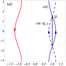
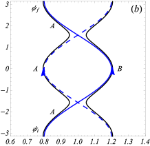
Figure 1: a) A modulation at a transverse wave vector ${\boldsymbol{Q}}_{\perp}=(0,\pi/b)$ couples states on the same side of the FS. In a magnetic field, the coupled trajectories (blue and dashed blue) flow along the same direction. b) The opening of a gap creates two open warped sheets of the FS (black), with the possibility magnetic breakdown at $(k_{F},\pm\pi/(2b))$. An electron initially on the sheet A may travel along two interfering paths (AAA and ABA), leading to magnetic oscillations in the conductance, with a frequency proportional to $t_{b}$.

We first consider the existence of a transverse modulation with amplitude $\Delta_{\perp}$ at wave vector ${\boldsymbol{Q}}_{\perp}=(0,\pi/b)$, as could be induced by an anion modulation along the transverse $y$ direction created by the ordering of ClO₄ anions in (TMTSF)₂ClO₄. The modulation couples states on the same side of the FS (Fig. 1).

In the presence of a magnetic field ${B}$, the electrons experience a motion along an open FS and quantum oscillations are usually not expected for an open FS. However, the situation is different here since two open trajectories run at short distance in ${\boldsymbol{k}}$ space and magnetic breakdown near the points $(k_{F},\pm\pi/2b)$ is possible.Stark ; Uji96 ; Uji2

The potential $\Delta_{\perp}$ couples $|{\boldsymbol{k}}\rangle$ and $|{\boldsymbol{k}}-{\boldsymbol{Q}}_{\perp}\rangle$, that is states on the same side of the Fermi surface. For $k_{x}>0$, this coupling is described by the effective Hamiltonian

$${\cal H}_{A}({\boldsymbol{k}})=\left(\begin{array}[]{cc}\epsilon_{{\boldsymbol{k}}}&\Delta_{\perp}\\ \Delta_{\perp}&\epsilon_{{\boldsymbol{k}}-{\boldsymbol{Q}}_{\perp}}\\ \end{array}\right)$$ (2)

with $\epsilon_{{\boldsymbol{k}}}$ given by (1) and

$$\epsilon_{{\boldsymbol{k}}-{\boldsymbol{Q}}_{\perp}}=\hbar v_{F}(k_{x}-k_{F})+2t_{b}\cos k_{y}b-2t_{b}^{\prime}\cos 2k_{y}b\ .$$ (3)

The $t^{\prime}_{b}$ term only slightly distorts the FS, but does not change the physics at all. Therefore we set here $t^{\prime}_{b}=0$. The new spectrum is given by

$$E_{{\boldsymbol{k}}}=\hbar v_{F}(k_{x}-k_{F})\pm\sqrt{\Delta_{\perp}^{2}+4t_{b}^{2}\cos^{2}k_{y}b}$$ (4)

and the equation of the corresponding FS ($E_{\boldsymbol{k}}=0$) is

$$k_{x}=k_{F}\pm{1\over\hbar v_{F}}\sqrt{4t_{b}^{2}\cos^{2}k_{y}b+\Delta_{\perp}^{2}}\ .$$ (5)

It is shown on Fig.1. It consists in two warped sheets along the same side of the FS.

III.1 Open orbits and magnetic breakdown

We estimate now the probability of magnetic breakdown in the vicinity of the gap separating these two sheets. Near the Bragg reflexion $k_{y}=\pm\pi/(2b)$, and expanding $k_{y}=\xi\pi/(2b)+q_{y}$ with $\xi=\pm 1$, the Hamiltonian has the form :

$${\cal H}_{A}(q_{y})=\left(\begin{array}[]{cc}2\xi t_{b}b\,q_{y}&\Delta_{\perp}\\ \Delta_{\perp}&-2\xi t_{b}b\,q_{y}\\ \end{array}\right)$$ (6)

with the spectrum

$$E_{{\boldsymbol{k}}}=\pm\sqrt{\Delta_{\perp}^{2}+4t_{b}^{2}b^{2}q_{y}^{2}}\ .$$ (7)

We define the transverse velocity as $\hbar v_{y}=2t_{b}b$. In a magnetic field ${B}$, the transverse wave vector $q_{y}$ varies linearly with the field, due to the Lorentz force $F=ev_{F}{B}$

$$\hbar q_{y}=ev_{F}{B}t$$ (8)

so that the time dependent Hamiltonian simply reads

$${\cal H}_{A}(t)=\left(\begin{array}[]{cc}\xi v_{y}Ft&\Delta_{\perp}\\ \Delta_{\perp}&-\xi v_{y}Ft\\ \end{array}\right)\ .$$ (9)

This problem is exactly equivalent to the Landau-Zener problem associated with the one-dimensional adiabatic spectrumLZ

$$E(t)=\pm\sqrt{\Delta_{\perp}^{2}+v_{y}^{2}F^{2}t^{2}}\ .$$ (10)

It is known that in this case, the Landau-Zener probability is therefore given by (the gap being $2\Delta_{\perp}$) :LZ

$$p_{\perp}\equiv e^{-2\pi\delta}=e^{\displaystyle-\pi{\Delta_{\perp}^{2}\over\hbar v_{y}F}}\ .$$ (11)

$\delta$ is called the adiabaticity parameter. In our case, the MB probability is given by

$$p_{\perp}=e^{\displaystyle-{{B}_{\perp}\over{B}}}\quad\mbox{with}\quad{B}_{\perp}=\pi{\Delta_{\perp}^{2}\over e\hbar v_{y}v_{F}}={\pi\over 2}{\Delta_{\perp}^{2}\over et_{b}bv_{F}}\ .$$ (12)

which is of the form found in Schoenberg (eq. 7.13).Schoenberg ; Blount At this stage, it is useful to compare this result with similar but different formulas used in the literature for $p_{\perp}$. In Ref.[Uji96, ], Uji et al. address the rapid oscillations in (TMTST)₂ ClO₄. The RO in the metallic phase are attributed to the Stark-Stückelberg mechanism that we discuss below. The characteristic field for magnetic breakdown is evaluated as ${B}_{\perp}={\Delta_{\perp}^{2}m_{c}\over\hbar e\epsilon_{F}}$ where $m_{c}$ is a cyclotron effective mass defined as $m_{c}=\hbar/(ev_{F}b)$ and assumed to be of the order of the free electron mass. Our result disagrees with this estimate since the energy scale in the denominator is proportional to $t_{b}$ and not to $\epsilon_{F}\propto t_{a}$. In Ref.[Uji2, ], a slightly more refined formula ${B}_{\perp}={\Delta_{\perp}^{2}m^{*}\over\hbar e\epsilon_{F}\sin(2\theta)}$ is in qualitative agreement with our result since $\theta$ is defined as the scattering angle at the gap, and is therefore of order $t_{b}/t_{a}$.

III.2 Stark-Stückelberg oscillations

Due to the modulation at wave vector ${\boldsymbol{Q}}_{\perp}$, one side of the FS is now made of two open sheets. In a magnetic field, the electrons travel on both sheets along the same direction, and possibly experience a tunneling through magnetic breakdown from one sheet to the other. Since this tunneling occurs in two different places (Fig. 1-b), the contributions corresponding to the two different paths may interfere. This phenomenon occurring between two LZ transitions is known as Stückelberg oscillations.Stuckelberg In the context of electronic magnetic breakdown, it has been proposed by Stark et al. to explain quantum oscillations in Mg,Stark and by Uji et al. do interpret the rapid resistance oscillations in the Bechgaard salt (TMTST)₂ ClO₄.Uji96 ; Uji97 We present here a quantitative picture of this effect.

Consider an electron in a magnetic field along one open sheet of the FS. During one period along the BZ, it experiences two LZ transitions to the neighboring sheet (Fig. 1-b). The tunnel probability amplitude $\sqrt{p_{\perp}}$ has been calculated above (12). The probability amplitude to stay on the same band is $\sqrt{1-p_{\perp}}$. Therefore calling $\psi_{i}$ the wave function on one sheet at one end of the BZ, the wave function $\psi_{f}$ on the same sheet at the other end is :

$$\psi_{f}=[p_{\perp}e^{i\phi_{B}}+(1-p_{\perp})e^{i(\phi_{A}-2\varphi_{s})}]\,\psi_{i}\ .$$ (13)

The first term corresponds to two ”transmissions” from one sheet (A, see Fig. 1-b) to the neighboring one (B), the second term corresponds to two reflections to the initial sheet (A). The phase $\phi_{A,B}={1\over\hbar}\int E_{A,B}(t)dt$ is the dynamical phase along the path $A,B$ between the two MB events. The phase $\varphi_{s}$ depends on the adiabaticity parameter $\delta$, therefore on the amplitude of the magnetic field. It is the so-called Stokes phase accumulated at a Landau-Zener reflection : $\varphi_{s}=\pi/4+\delta(\ln\delta-1)+\mbox{arg}\Gamma(1-i\delta)$.Shevchenko Here, we have $2\pi\delta={B}_{\perp}/{B}$. Therefore $\varphi_{s}$ varies between $0$ in the adiabatic limit ($\delta\rightarrow\infty$, absence of magnetic breakdown, ${B}\ll{B}_{\perp}$) to $\pi/4$ in the diabatic limit ($\delta\rightarrow 0$, strong magnetic breakdown, ${B}\gg{B}_{\perp}$). From (13), the probability for the electron to stay on the same sheet after one period is therefore given by :

$$|\psi_{f}|^{2}/|\psi_{i}|^{2} = p_{\perp}^{2}+(1-p_{\perp})^{2}$$ (14)

$$+ 2p_{\perp}(1-p_{\perp})\cos(\phi+2\varphi_{s})$$ (15)

where $\phi=\phi_{B}-\phi_{A}$ is the magnetic field dependent dynamical phase accumulated between the two paths. It is given by $\phi={1\over\hbar}\int_{-t_{0}}^{t_{0}}\Delta E(t)dt$ with $\Delta E(t)=2\sqrt{\Delta_{\perp}^{2}+4t_{b}^{2}\cos^{2}{ev_{F}b{B}t\over\hbar}}$ and $ev_{F}b{B}t_{0}/\hbar=\pi/2$. In the limit, $\Delta_{\perp}\ll t_{b}$, the dynamical phase is simply given by $\phi(0)={8t_{b}\over ev_{F}b{B}}$. It increases with $\Delta_{\perp}$ as $\phi(\Delta_{\perp})=\phi(0)F_{\perp}(\Delta_{\perp}/2t_{b})$ where the function $F_{\perp}(x)$ is given by

$$F_{\perp}(x)=\int_{0}^{\pi/2}\sqrt{\cos^{2}t+x^{2}}\,dt\ .$$ (16)

This interference mechanism leads to oscillations of the conductivity of the form :Stark

$$\sigma_{osc}\propto 2p_{\perp}(1-p_{\perp})\cos(2\pi{{B_{f}}\over{B}}+2\varphi_{s})\ ,$$ (17)

where the the characteristic field ${B}^{*}$ is

$${B_{f}}(\Delta_{\perp})={4t_{b}\over\pi ev_{F}b}\ F_{\perp}\left({\Delta_{\perp}\over 2t_{b}}\right)\ .$$ (18)

It increases with $\Delta_{\perp}$ since the distance between interfering orbits increases in ${\boldsymbol{k}}$ space. It is plotted in Fig. 2.

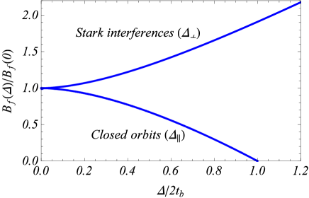
Figure 2: Gap dependence of the characteristic field ${B_{f}}$ of the rapid oscillations, for a transverse modulation $\Delta_{\perp}$ leading to Stark interferences and for a longitudinal modulation $\Delta_{\parallel}$ leading to closed quantized orbits (see Eqs.18, 24). This corresponds to the situation respectively encountered in (TMTSF)₂ClO₄ and (TMTSF)₂ReO₄ under pressure on the one hand, and (TMTSF)₂NO₃ at ambient pressure on the other hand, as discussed in the summary section (IX).

As already explained in Refs.[Stark, ; Uji96, ; Uji2, ], these oscillations are only visible in transport and they ressemble Shubnikov-de Haas oscillation, however with a different temperature dependence. Since the dynamical phase is energy independent (it does not depend on the position of the Fermi energy), there is no thermal damping of the oscillations. Their temperature dependence is due to that of the scattering time.Uji96

Since these quantum oscillations involve two LZ transitions, they vanish for a large gap $\Delta_{\perp}$ ($p_{\perp}\rightarrow 0$) and also for small gap ($p_{\perp}\rightarrow 1$). They vary as :

$$\sigma_{osc}\propto e^{-{B}_{\perp}/{B}}\left(1-e^{-{B}_{\perp}/{B}}\right)\cos\left(2\pi{{B_{f}}\over{B}}+2\varphi_{s}\right)\ .$$ (19)

Typical variations are shown on Fig.3. They are maximal for $p_{\perp}=1/2$, that is for a field $B_{m}=B_{\perp}/\ln 2$. This mechanism has been proposed as a possible explanation for the rapid oscillations observed in the metallic phase of (TMTSF)₂ClO₄.Uji96 ; Uji97 With the known physical parameters in this salt, $a=3.65\AA$, $b=7.7\AA$, $t_{a}\simeq 3000$ K, $t_{b}\simeq 300$ K, and a recent estimateAlemany14 of the anion gap $\Delta_{\perp}\simeq 14$ meV, one finds an order of magnitude $B_{\perp}\simeq 40$ T which is compatible with experiments. The same mechanism should also explain the RO in (TMTSF)₂ReO₄ which seem to be of the same nature.Kang91b For completion, let us mention ref.[eescattering, ] which argues that the effect is too small and proposes another mechanism related to the modulation of electron-electron scattering in the presence of a magnetic field.

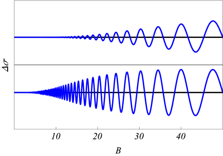
Figure 3: Evolution of the Stark oscillations in a magnetic field (arbitrary units). Here we have taken ${B_{f}}=250$ T, ${B}_{\perp}=70$ T (top curve) and ${B}_{\perp}=30$ T (bottom curve).

IV Longitudinal $(2k_{F},0)$ modulation

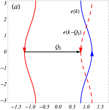
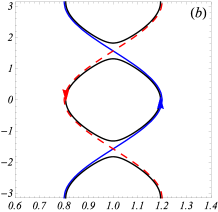
Figure 4: a) A modulation at a parallel wave vector ${\boldsymbol{Q}}_{\parallel}=(2k_{F},0)$ couples opposite sides of the FS. In a magnetic field, the coupled trajectories have opposite signs (blue and dashed red). b) The opening of a gap at this wavevector creates electron and hole closed pockets (black), whose motion is quantized, leading to SdH oscillations with frequency $t_{b}$. The magnetic breakdown broadens Landau levels.

We now consider the existence of a longitudinal modulation with amplitude $\Delta_{\parallel}$ at wave vector ${\boldsymbol{Q}}_{\parallel}=(2k_{F},0)$, as it exists in (TMTSF)₂NO₃ under pressure.Kang95 ; Vignolles05 This case is quite different from the previous one, since the modulation vector ${\boldsymbol{Q}}_{\parallel}=(2k_{F},0)$ couples states on opposite sheets of the Fermi surface (Fig. 4-a). The corresponding Hamiltonian has the form :

$${\cal H}_{\parallel}({\boldsymbol{k}})=\left(\begin{array}[]{cc}\epsilon_{\boldsymbol{k}}&\Delta_{\parallel}\\ \Delta_{\parallel}&\epsilon_{{\boldsymbol{k}}-{\boldsymbol{Q}}_{\parallel}}\\ \end{array}\right)$$ (20)

with

$$\epsilon_{{\boldsymbol{k}}-{\boldsymbol{Q}}_{\parallel}}=-\hbar v_{F}(k_{x}-k_{F})-2t_{b}\cos k_{y}b-2t_{b}^{\prime}\cos 2k_{y}b$$ (21)

to be compared with (3) where the modulation was at wave vector ${\boldsymbol{Q}}_{\perp}=(0,\pi/b)$. Like in the previous case, the $t^{\prime}_{b}$ term does not play an important role here, and we set $t^{\prime}_{b}=0$. The spectrum is given by

$$E_{\boldsymbol{k}}=-2t_{b}\cos(k_{y}b)\pm\sqrt{\Delta^{2}+\hbar^{2}v_{F}^{2}(k_{x}-k_{F})^{2}}$$ (22)

and the equation of the FS ($E_{\boldsymbol{k}}=0$) is :

$$k_{x}=k_{F}\pm{1\over\hbar v_{F}}\sqrt{4t_{b}^{2}\cos^{2}k_{y}b-\Delta_{\parallel}^{2}}$$ (23)

to be contrasted with (5) for the ${\boldsymbol{Q}}_{\perp}$ modulation. The Fermi surface is shown on Fig. 4-b. It defines electron and holes pockets of equal size, leading to closed orbits in a magnetic field.Fortin2009 The area of these orbits is ${\cal A}={8t_{b}\over\hbar v_{F}b}$ leading to Shubnikov-de Haas oscillations with a characteristic field) :

$${B_{f}}(\Delta_{\parallel})={4t_{b}\over\pi ev_{F}b}\ F_{\parallel}(\Delta_{\parallel}/2t_{b})\ ,$$ (24)

with

$$F_{\parallel}(x)=\int_{0}^{\arccos x}\sqrt{\cos^{2}t-x^{2}}\,dt\ .$$ (25)

For a small gap, this is the same characteristic field as in the previous case. However, it decreases when the gap increases, since the size of the closed pockets decreases. The variation is shown on Fig. 2. It is indeed interesting to contrast the gap ($\Delta_{\parallel}$) dependence of the characteristic field of these SdH oscillations, with the gap ($\Delta_{\perp}$) dependence of the characteristic field of the Stark oscillations.

Due to magnetic breakdown, there is a finite probability of tunneling between the closed orbits shown on Fig. 4-b, leading to open orbits. To calculate this probability, we expand the Hamiltonian near a crossing point $k_{y}=\xi\pi/(2b)+q_{y}$ with $\xi=\pm 1$. It takes the form

$${\cal H}_{\parallel}=\left(\begin{array}[]{cc}\delta+2\xi t_{b}b\,q_{y}&\Delta_{\parallel}\\ \Delta_{\parallel}&-\delta+2\xi t_{b}b\,q_{y}\\ \end{array}\right)$$ (26)

with the spectrum ($\delta=v_{F}(k_{x}-k_{F})$)

$$E_{\boldsymbol{k}}=2\xi t_{b}bq_{y}\pm\sqrt{\delta^{2}+\Delta_{\parallel}^{2}}\ .$$ (27)

In a magnetic field, there is a key difference with the previous case since the motion is opposite along the two sheets of the Fermi surface :

$$\hbar q_{y}=\pm Ft=ev_{F}{B}t$$ (28)

with $\hbar v_{y}=2t_{b}b$. Therefore the time dependent Hamiltonian reads

$${\cal H}_{\parallel}(t)=\left(\begin{array}[]{cc}\xi v_{y}Ft&\Delta_{\parallel}\\ \Delta_{\parallel}&-\xi v_{y}Ft\\ \end{array}\right)$$ (29)

and the LZ probability to tunnel from one closed pocket to another is given by

$$p_{\parallel}=e^{\displaystyle-{{B}_{\parallel}\over{B}}}\quad\mbox{with}\quad{B}_{\parallel}=\pi{\Delta_{\parallel}^{2}\over e\hbar v_{y}v_{F}}={\pi\over 2}{\Delta_{\parallel}^{2}\over et_{b}bv_{F}}\ .$$ (30)

This magnetic breakdown leads to a broadening of the Landau levels $E_{n}=(n+1/2)ev_{F}b{B}$, which has been estimated by different methods in Refs.[Gvozdikov, ; Fortin2009, ]. This broadening leads to a modulation of the SdH oscillations.

V $(2k_{F},\pi/b)$ Nesting ordering

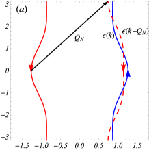
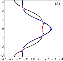
Figure 5: a) A modulation at the nesting vector ${\boldsymbol{Q}}_{N}=(2k_{F},\pi/b)$ couples opposite sides of the FS. In a magnetic field, the coupled trajectories flow along opposite directions (blue and red dashed). b) The opening of a gap at this wavevector creates electronic closed pockets (black), whose motion is quantized, leading to SdH oscillations with frequency proportional to $t^{\prime}_{b}$.

Like in the previous case, this modulation couples states on opposite sheets of the Fermi surface (Fig. 5-a). The difference is that the nesting of the FS is almost perfect,remarknesting and the characteristic field ${B_{f}}$ of the SdH oscillations is set by the energy scale $t^{\prime}_{b}$ instead of $t_{b}$. The Hamiltonian reads :

$${\cal H}_{N}({\boldsymbol{k}})=\left(\begin{array}[]{cc}\epsilon_{\boldsymbol{k}}&\Delta_{N}\\ \Delta_{N}&\epsilon_{{\boldsymbol{k}}-{\boldsymbol{Q}}_{N}}\\ \end{array}\right)$$ (31)

with

$$\epsilon_{{\boldsymbol{k}}-{\boldsymbol{Q}}_{N}}=-\hbar v_{F}(k_{x}-k_{F})+2t_{b}\cos k_{y}b-2t_{b}^{\prime}\cos 2k_{y}b$$ (32)

to be compared with (3). The spectrum is given by

$$E_{\boldsymbol{k}}=-2t_{b}^{\prime}\cos(2k_{y}b)\pm\sqrt{\Delta_{N}^{2}+[\hbar v_{F}(k_{x}-k_{F})-2t_{b}\cos k_{y}b]^{2}}$$ (33)

and is shown on Fig. (5-b). The equation of the FS is

$$k_{x}=k_{F}-{2t_{b}\over v_{F}}\cos k_{y}b\pm{1\over v_{F}}\sqrt{4{t^{\prime}_{b}}^{2}\cos^{2}2k_{y}b-\Delta_{N}^{2}}\ .$$ (34)

The Fermi surface consists in four inequivalent small electron pockets, leading to closed orbits in a magnetic field. However due to magnetic breakdown there is a finite probability of tunneling between these orbits, leading to larger or even open orbits. To calculate this probability, we expand the Hamiltonian near a crossing point $k_{y}=\xi\pi/(4b)+q_{y}$ with $\xi=\pm 1$. It takes the form

$${\cal H}_{N}({\boldsymbol{k}})=\left(\begin{array}[]{cc}\delta-4\xi t_{b}^{\prime}b\,q_{y}&\Delta_{N}\\ \Delta_{N}&\delta-4\xi t_{b}^{\prime}b\,q_{y}\\ \end{array}\right)$$ (35)

with the spectrum ($\delta=v_{F}(k_{x}-k_{F})-t_{b}\sqrt{2}$)

$$E_{\boldsymbol{k}}=-4\xi t_{b}^{\prime}bq_{y}\pm\sqrt{\delta^{2}+\Delta_{N}^{2}}\ .$$ (36)

In a magnetic field, the motion is opposite along the two sheets of the Fermi surface :

$$q_{y}=\pm Ft=ev_{F}{B}t$$ (37)

with $\hbar v_{y}^{\prime}=4t_{b}^{\prime}b$. Therefore the time dependent Hamiltonian reads

$${\cal H}_{N}(t)=\left(\begin{array}[]{cc}-\xi v_{y}^{\prime}Ft&\Delta_{N}\\ \Delta_{N}&\xi v_{y}^{\prime}Ft\\ \end{array}\right)\ .$$ (38)

The LZ probability to tunnel between closed orbits is therefore given by

$$p_{N}=e^{\displaystyle-{{B}_{N}\over{B}}}\quad\mbox{with}\quad{B}_{N}=\pi{\Delta_{N}^{2}\over\hbar v_{y}^{\prime}F}={\pi\over 4}{\Delta_{N}^{2}\over et_{b}^{\prime}bv_{F}}\ .$$ (39)

This tunneling leads to a broadening of the Landau levels and to a modulation of the SdH oscillations.Gvozdikov These slow oscillations have been not observed yet in the SDW phase of Q-(TMTSF)₂ClO₄ or (TMTSF)₂PF₆.

VI Nesting ordering and transverse modulation

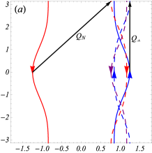
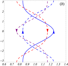
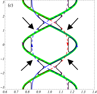
Figure 6: a) The presence of the two modulations ${\boldsymbol{Q}}_{N}=(2k_{F},\pi/b)$ and ${\boldsymbol{Q}}_{\perp}=(0,\pi/b)$ couples four states (${\boldsymbol{k}}$ blue, ${\boldsymbol{k}}-{\boldsymbol{Q}}_{N}$ dashed red, ${\boldsymbol{k}}-{\boldsymbol{Q}}_{\perp}$ dashed blue and ${\boldsymbol{k}}-{\boldsymbol{Q}}_{\perp}+{\boldsymbol{Q}}_{N}$ dashed purple), creating six electronic closed pockets (black) (b) whose motion is quantized, leading to SdH oscillations with frequency $t^{\prime}_{b}$. Notice the existence of new $X$-shape pockets. Magnetic breakdown through the gaps (arrows) leads to large closed orbits (shown in green in the bottom figure c) whose size is proportional to $t_{b}$.

We consider now the case where two periodicities coexist, one at wave vector ${\boldsymbol{Q}}_{N}=(2k_{F},\pi/b)$ with amplitude $\Delta_{N}$, and one at wave vector ${\boldsymbol{Q}}_{\perp}=(0,\pi/b)$ with amplitude $\Delta_{\perp}$. This could be the case for example if a DW and a modulation due to anion ordering would coexist, as in the anion ordered phase of (TMTSF)₂ClO₄. This situation has been studied extensively in Ref.[Machida97, ], and we present here a simple analytical description. It first has to be stressed that this situation cannot be reduced to the case of one modulation at wave vector ${\boldsymbol{Q}}_{N}-{\boldsymbol{Q}}_{\perp}$. This is a novel situation in which four states are coupled. Indeed these two modulations couple a state with wavevector ${\boldsymbol{k}}$ to a infinity of states ${\boldsymbol{k}}+m{\boldsymbol{Q}}_{N}+n{\boldsymbol{Q}}_{\perp}$. Considering states closed to the FS, one sees that a vector ${\boldsymbol{k}}$ on the right side of the FS is coupled to ${\boldsymbol{k}}-{\boldsymbol{Q}}_{N}$, ${\boldsymbol{k}}-{\boldsymbol{Q}}_{\perp}$ and ${\boldsymbol{k}}-{\boldsymbol{Q}}_{N}+{\boldsymbol{Q}}_{\perp}$. The energy spectrum $E_{\boldsymbol{k}}$ is therefore given by the eigenvalues of the Hamiltonian :

$${\cal H}({\boldsymbol{k}})=\left(\begin{array}[]{cccc}\epsilon_{{\boldsymbol{k}}}&\Delta_{{\boldsymbol{Q}}_{N}}&\Delta_{{\boldsymbol{Q}}_{\perp}}&0\\ \Delta_{{\boldsymbol{Q}}_{N}^{*}}&\epsilon_{{\boldsymbol{k}}-{\boldsymbol{Q}}_{N}}&0&\Delta_{{\boldsymbol{Q}}_{\perp}}\\ \Delta_{{\boldsymbol{Q}}_{\perp}^{*}}&0&\epsilon_{{\boldsymbol{k}}-{\boldsymbol{Q}}_{\perp}}&\Delta_{{\boldsymbol{Q}}_{N}}\\ 0&\Delta_{{\boldsymbol{Q}}_{\perp}^{*}}&\Delta_{{\boldsymbol{Q}}_{N}^{*}}&\epsilon_{{\boldsymbol{k}}-{\boldsymbol{Q}}_{N}+{\boldsymbol{Q}}_{\perp}}\\ \end{array}\right)\ .$$ (40)

Fig.6-a shows the four states which are coupled by the modulations, with opening of a gap near $k_{y}=\pm\pi/(4b)$ and $k_{y}=\pm 3\pi/(4b)$, as seen on Fig. 6-b. The new spectrum exhibits two kinds of electronic pockets : pockets with a banana shape as in the case of pure DW modulation and new pockets with a X-shape. Quantization of these orbits in a field should lead to oscillations with frequency $t^{\prime}_{b}$. The important new feature here is the possibility of magnetic breakdown through four gaps, leading to closed orbits of large size, related to $t_{b}$ (Fig. 6-c) leading therefore to rapid quantum oscillations. The probability of having such large orbits involves four magnetic breakdowns (shown by arrows in Fig. 6-c with probability $p_{N}$ calculated above (Eq. 39) and two Bragg reflections. The amplitude associated to the Bragg reflection may be more difficult to calculate since it involves four waves instead of two. This scenario is therefore expected to lead to rapid oscillations superimposed to the slow oscillations. It naturally explains the existence of thermodynamic rapid oscillations in the FISDW of R-(TMTSF)₂ClO₄,Kang91b ; Uji96 as well as in (TMTSF)₂ReO₄ under pressureSchwenk86 ; Kang91b .

VII Nesting ordering and longitudinal modulation

In this situation, two periodicities coexist, one corresponding to a DW ordering at wave vector ${\boldsymbol{Q}}_{N}=(2k_{F},\pi/b)$ and a modulation at the longitudinal wave vector ${\boldsymbol{Q}}_{\parallel}=(2k_{F},0)$ as the one induced by the anion ordering in (TMTSF)₂NO₃. As in the previous case, four states are coupled close to the Fermi level, ${\boldsymbol{k}}$, ${\boldsymbol{k}}-{\boldsymbol{Q}}_{N}$, ${\boldsymbol{k}}-{\boldsymbol{Q}}_{\parallel}$ and ${\boldsymbol{k}}-{\boldsymbol{Q}}_{N}+{\boldsymbol{Q}}_{\parallel}$. This situation is therefore very similar to the previous one, since one has ${\boldsymbol{Q}}_{\parallel}={\boldsymbol{Q}}_{N}-{\boldsymbol{Q}}_{\perp}$, and the Fermi pockets in this case resemble those presented in Fig.6.Machida97 One expects a superposition of rapid oscillations related to the large pockets due to magnetic breakdown between small pockets responsible for slow oscillations. This scenario naturally explains the two series of oscillations observed in the SDW phase of (TMTSF)₂NO₃.Audouard94 ; Kang95 ; Vignolles05

VIII Two commensurate SDW

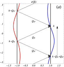
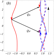
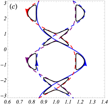
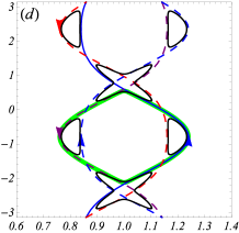
Figure 7: Fermi surface related to the dispersion relation (42), and modulation wave vectors ${\boldsymbol{Q}}_{N}=(2k_{F},\pi/2b)$ and ${\boldsymbol{Q}}_{N^{\prime}}=(2k_{F},-\pi/2b)$. a) The presence of these two modulations couples four states, couples four states (${\boldsymbol{k}}$ blue, ${\boldsymbol{k}}-{\boldsymbol{Q}}_{N}$ dashed red, ${\boldsymbol{k}}-{\boldsymbol{Q}}_{N^{\prime}}$ dashed purple and ${\boldsymbol{k}}-{\boldsymbol{Q}}_{N}+{\boldsymbol{Q}}_{N^{\prime}}$ dashed blue), creating six electronic closed pockets (b) whose motion is quantized, leading to SdH oscillations with frequency $t^{\prime}_{b}$. Notice the existence of new $X$-shape pockets. Magnetic breakdown through the gaps leads to closed orbits (green curve in d) whose size is proportional to $t_{b}$.

The two previous sections show interesting situations when two modulations coexist. This is the case in (TMTSF)₂ClO₄ and (TMTSF)₂NO₃, where a DW modulation coexists with a modulation due to anion ordering, respectively at wave vectors ${\boldsymbol{Q}}_{\parallel}=(0,\pi/b)$ and ${\boldsymbol{Q}}_{\perp}=(2k_{F},0)$. However, rapid oscillations may also exist even in the absence of anion ordering, as it is the case in (TMTSF)₂PF₆. We now discuss another situation where two DW modulations can coexist, leading to a similar structure of the FS as in the two previous sections. Instead of the orthorhombic symmetry considered until now, we consider the triclinic symmetry pertinent to Bechgaard salts. The FS is distorted such that the two sheets are not facing each other as in the previous cases, but one is shifted with respect to the other one (Fig. 7-a). Here we keep the same simple orthorhombic model where the shift is described by a phase $\phi$ :Yamajibook

$$\epsilon({\boldsymbol{k}}) = \hbar v_{F}(|k_{x}|-k_{F})-2t_{b}\cos[k_{y}b+\phi~{}\mbox{sgn}(k_{x})]$$ (41)

$$- 2t_{b}^{\prime}\cos[2k_{y}b+2\phi~{}\mbox{sgn}(k_{x})]\ .$$ (42)

We consider the commensurate situation when the shift $\phi=\pi/4$ as shown on Fig. 7-a.

Assume the existence of a modulation close to perfect nesting at wave vector ${\boldsymbol{Q}}_{N}=(2k_{F},\pi/2b)$, which couples states ${\boldsymbol{k}}$ and ${\boldsymbol{k}}-{\boldsymbol{Q}}_{N}$. Consider also the modulation at wave vector ${\boldsymbol{Q}}_{N^{\prime}}=(2k_{F},-\pi/2b)$ which does not provide a so good nesting. However, the state ${\boldsymbol{k}}-{\boldsymbol{Q}}_{N^{\prime}}$ is coupled to the state ${\boldsymbol{k}}+{\boldsymbol{Q}}_{N^{\prime}}-{\boldsymbol{Q}}_{N}$ which is close to the FS. Therefore, we have to consider the coupling between four states near the Fermi level ${\boldsymbol{k}}$, ${\boldsymbol{k}}-{\boldsymbol{Q}}_{N}$, ${\boldsymbol{k}}-{\boldsymbol{Q}}_{N^{\prime}}$, ${\boldsymbol{k}}-{\boldsymbol{Q}}_{N}+{\boldsymbol{Q}}_{N^{\prime}}$.remarkcommensurate The coupling vectors are represented on Fig. 7-b.

Let $\Delta_{N}$ and $\Delta_{N^{\prime}}<\Delta_{N}$ be the amplitude of these two modulations. The new spectrum is obtained by diagonalization of the $4\times 4$ matrix :

$${\cal H}({\boldsymbol{k}})=\left(\begin{array}[]{cccc}\epsilon_{{\boldsymbol{k}}}&\Delta_{N}&\Delta_{N^{\prime}}&0\\ \Delta_{N}^{*}&\epsilon_{{\boldsymbol{k}}-{\boldsymbol{Q}}_{N}}&0&\Delta_{N^{\prime}}^{*}\\ \Delta_{N^{\prime}}^{*}&0&\epsilon_{{\boldsymbol{k}}-{\boldsymbol{Q}}_{N^{\prime}}}&\Delta_{N}^{*}\\ 0&\Delta_{N^{\prime}}&\Delta_{N}&\epsilon_{{\boldsymbol{k}}-{\boldsymbol{Q}}_{N}+{\boldsymbol{Q}}_{N^{\prime}}}\\ \end{array}\right)\ .$$ (43)

It appears clearly that this model is very similar to the one discussed in section III, ${\boldsymbol{Q}}_{N}-{\boldsymbol{Q}}_{N^{\prime}}$ playing the same role as ${\boldsymbol{Q}}_{\perp}$  : four states are coupled and we have the correspondance (compare (43) with the Hamiltonian (40)) :

${\boldsymbol{Q}}_{N}=(2k_{F},\pi/b)$	$\longleftrightarrow$	${\boldsymbol{Q}}_{N}=(2k_{F},\pi/2b)$
${\boldsymbol{Q}}_{\perp}=(0,\pi/b)$	$\longleftrightarrow$	${\boldsymbol{Q}}_{N}-{\boldsymbol{Q}}_{N^{\prime}}=(0,\pi/b)$
${\boldsymbol{Q}}_{N}-{\boldsymbol{Q}}_{\perp}=(2k_{F},0)$	$\longleftrightarrow$	${\boldsymbol{Q}}_{N^{\prime}}=(0,-\pi/2b)$

Like in the two previous cases, there are two kinds of closed Fermi pockets, shown on Fig.7-c, whose size is typically related to $t^{\prime}_{b}$ so that one should expect also slow oscillations. Magnetic breakdown through the gaps leads to large trajectories (shown in green in Fig.7-d), whose size is related to $t_{b}$ and which may lead to RO. This mechanism may actually be strengthened by Umpklapp processes due to the commensurability condition ${\boldsymbol{Q}}_{N}+{\boldsymbol{Q}}_{N^{\prime}}=(4k_{F},0)=(2\pi/a,0)$ as proposed by Lebed.Lebed91 This scenario has been proposed in a qualitative form in Ref. [Uji2, ]. It provides a satisfactory explanation for the RO observed in (TMTSF)₂PF₆. In this salt, it has been found that the characteristic field ${B_{f}}$ increases with pressure in a way which supports the proportionality between ${B_{f}}$ and $t_{b}$.Kornilov07 The slow oscillations related to the small pockets may be difficult to observe. The RO being due to magnetic breakdown induced closed orbits are also expected in magnetization experiments, but have not been observed.Uji2

IX Summary and discussion

Quantum oscillations in quasi-1D conductors with an open Fermi surface originate from a reconstruction of the FS due to potentials induced by periodic modulations. Their nature can be classified by their characteristic frequency – or characteristic magnetic field ${B_{f}}$. The frequency of the rapid oscillations is typically related to the energy $t_{b}$ which describes the warping of the FS. The slow oscillations are related to the energy scale $t^{\prime}_{b}$ which measures the deviation from the sinusoidal warping. This paper is a review of different mechanisms which may lead to the RO. The table (8) summarizes such mechanisms which may explain different types of RO in the Bechgaard salts.

	metallic	SDW
R-ClO4/ReO4	${\boldsymbol{Q}}_{\perp}$ (Stark, III)	${\boldsymbol{Q}}_{\perp}$​ and​ ${\boldsymbol{Q}}_{N}$​ (VI)
NO3 low pressure	${\boldsymbol{Q}}_{\parallel}$(IV)	${\boldsymbol{Q}}_{\parallel}$​ and​ ${\boldsymbol{Q}}_{N}$​ (VII)
NO3 high pressure	${\boldsymbol{Q}}_{\perp}$(III)​	${\boldsymbol{Q}}_{\perp}$​ and​ ${\boldsymbol{Q}}_{N}$​ (VI)
PF6/AsF6/Q-ClO4		${\boldsymbol{Q}}_{N}$​ and​ ${\boldsymbol{Q}}_{N^{\prime}}$​ (VIII)

Figure 8: Possible scenarios to explain the fast oscillations in the TMTSF salts. We refer to the coupling vectors associated to each scenario and the corresponding section in the paper. Here ReO₄ is under pressure. For NO₃, low and high pressure refer respectively to pressures lower and higher than $7$ kbar.

$\bullet$ The simplest mechanisms, described in sections III and IV, involve only one periodic modulation modulation.

A transverse modulation ($\Delta_{\perp}$) at wave vector $(2k_{F},\pi/b)$ induces a pair of trajectories on the same side of the FS which may interfere via MB, and realize Stückelberg oscillations which, in the context of magnetic oscillations, have first been proposed by Stark and Friedberg.Stark ; Uji96 ; Uji97 This modulation is induced by anion ordering in R-$\mathrm{ClO_{4}}$ at ambient pressureYan87 ; Kang91b ; Uji96 or in $\mathrm{ReO_{4}}$ under pressure.Schwenk86 The characteristic fields of the oscillations are respectively ${B_{f}}=265$ T and ${B_{f}}=290$ T. Due to this particular interference mechanism, these oscillations are observed solely on the conductivity but not on thermodynamic properties.

A longitudinal modulation ($\Delta_{\parallel}$) at wave vector $(2k_{F},0)$ couples states on opposite side and the reconstructed FS has closed Fermi pockets, the size of which is proportional to $t_{b}$. This is the case in $\mathrm{NO_{3}}$ at ambient pressure, with the anion ordering yielding a potential at wave vector $(2k_{F},0)$.Kang95 ; Vignolles05

The evolution of the characteristic field ${B_{f}}$ with the gap induced by the modulation may be easily calculated in these two previous scenarios (sections III, IV). In the first case, it increases with the amplitude of the gap $\Delta_{\perp}$ while it decreases with the gap $\Delta_{\parallel}$ in the second case (Fig. 2). This is consistent with the observation of a smaller frequency in $\mathrm{NO_{3}}$ at ambient pressure (${B_{f}}=248$ T)Kang95 ; Vignolles05 compared to the cases of $\mathrm{ClO_{4}}$ (${B_{f}}=255-265$ T)Brooks99 ; Yan87 ; Chaikin83 or $\mathrm{ReO_{4}}$  (${B_{f}}=320-330$ T) under pressure.Schwenk86 ; Kang95 ; Vignolles05

$\bullet$ More complex scenarios involve the superposition of two modulations, that is two order parameters with probably different amplitudes, a nesting modulation correlated to the apparition of a DW plus one of the two above-mentioned modulations related to an anion ordering. The reconstruction of the FS in these cases is quite rich. It exhibits closed FS with characteristic size related to size $t^{\prime}_{b}$ plus large trajectories induced by MB, the size of which is related to $t_{b}$. Therefore one expects a superposition of slow and rapid oscillations. Their respective amplitude may be difficult to predict theoretically, since it depends on the relative amplitude of the two order parameters and on the MB probability. This is the situation in R-ClO₄ where indeed RO have been observed in the FISDW. It is noticeable that the RO in the metallic phase are seen only in transport experiments while, in the FISDW phases, they are seen both in transport and thermodynamic measurement. This proves that the mechanism for RO is different in the presence of a single transverse modulation or in the presence of two modulations (transverse + SDW), as already noticed in Ref.Kang91b, .

$\bullet$ $\mathrm{(TMTSF)_{2}NO_{3}}$  is a particularly rich system. Rapid and slow oscillations are observed simultaneously in the low temperature and low pressure SDW phase,Audouard94 compatible with the superposition of a nesting modulation plus an anion-ordering induced modulation at wave vector $(2k_{F},0)$. The observed increase of the frequencies of both oscillation sequences is compatible with an increase of the characteristic energies $t_{b}$ and $t^{\prime}_{b}$ under pressure.Vignolles05

However, a surprising feature is the sharp drop of the characteristic frequency of the RO at a pressure of order 7 kbar from $325$ T to $215$ T, together with a vanishing of the slow oscillations. Such a jump is hardly understandable without an important structural change. Several arguments suggest an anion order evolving from ${\boldsymbol{Q}}_{\parallel}=(2k_{F},0)$ to ${\boldsymbol{Q}}_{\perp}=(0,\pi/b)$ around $7$ kbar. Firstly, the shape of the transport anomaly passing through the anion ordering changes drastically.Mazaud80 ; Kang90 Secondly, a recent investigation of the angular dependent magnetoresistance of $\mathrm{(TMTSF)_{2}NO_{3}}$  under 8.7 kbar has concluded to the existence of a Q1D Fermi surface even in the presence of anion ordering.Kang09 Thirdly, an ab-initio calculation is supporting these experimental findings.Alemany14 These arguments suggest a pressure induced phase transition from an anion induced modulation at wave vector $(2k_{F},0)$ and a modulation at wave vector $(0,\pi/b)$. Therefore, the RO reported at $\approx$ 8 kbarKang95 ; Vignolles05 might be actually related to Stark interferences between two sheets of folded Fermi surfaces like in R-$\mathrm{(TMTSF)_{2}ClO_{4}}$ . The possibility of a pressure induced structural transition could deserve further experimental and theoretical investigations.

$\bullet$ The existence of RO occurring in a SDW phase without any role played by anions, like in $\mathrm{PF_{6}}$, $\mathrm{AsF_{6}}$ or Q-$\mathrm{ClO_{4}}$, is more problematic since a pure SDW ordering is expected to induce only slow oscillations with frequency related to $t^{\prime}_{b}$. The mechanism at the origin of such RO may find its origin in the particular (triclinic) lattice symmetry of the Bechgaard salts. As a consequence of this triclinicity, the two sheets of the FS are actually shifted with respect to each other by a vector close to the commensurate value $(0,\pi/2b)$ so that naturally in the presence of a SDW two modulations at wave vectors $(2k_{F},\pm\pi/2b)$ may coexist.Uji2 ; Lebed91 This situation is not so different from those described earlier where a SDW and anion induced modulation coexist. We argue that this may explain the existence of RO in (TMTSF)₂PF₆ or Q-(TMTSF)₂ClO₄. This scenario assumes the existence of two commensurate SDWs, at wave vectors $(2k_{F},\pm\pi/2b)$, so that the coupling between relevant states at the Fermi level is described by a $4\times 4$ matrix. One may wonder if this commensurate model is a good approximation for the actual incommensurate situation. This is probably the case and given that the actual phase is close to commensurate, one expects that the SDW will exhibit discommensurations.

We close this conclusion by a discussion on open questions related to the commensurability of the SDW ordering in several Bechgaard salts.

Several experimental results provide hints for a commensurate SDW state in (TMTSF)₂PF₆. Strain and defect-free samples exhibit a first order transition with a sharp increase in the resistivity at $T_{SDW}\simeq 12$K. In addition, a non-linear conduction is the signature of a pinning mechanism due to fourfold commensurability Kang90 . A weakly first order transition is also the conclusion of a study of the ¹³C NMR linewidth through the transition.Clark01 Moreover signs of commensurability are also clearly provided by ¹³C NMR spectra.Nagata13 The examination of the ¹H-NMR lineshape has led to a determination SDW wave vector as $(\pi/a,\simeq\pi/2b)$ with a rather broad error bar for the transverse component.Delrieu86 ; Takahashi86b This is consistent with a triclinic symmetry, since the best nesting vector for a simplified orthorhombic model would be ($\pi/a,\pi/b$). However the typical double horn shape of the ¹³C-NMR spectra makes the existence of an incommensurate modulation undisputable at least in the temperature interval between 12K and 4K.Barthel93b ; Nagata13

Another puzzle concerns the anomalous behaviour in the temperature dependence of several properties in the ambient pressure SDW phases of (TMTSF)₂X salts. The purest samples exhibit a significant enhancement of the resistivity at 4K but more important, the amplitude of RO departs from the Lifshitz-Kosevich behaviour: : it has a sudden drop at $T^{\star}\approx 4$K without noticeable change of the frequency in $\mathrm{PF_{6}}$ , $\mathrm{AsF_{6}}$Ulmet85 and Q-$\mathrm{ClO_{4}}$.Brooks99 Interestingly, an anomalous behavior has also been noticed in the same temperature domain for the NMR properties namely, a sharp drop of protonTakahashi86a and ⁷⁷Se spin-lattice relaxation rates in $\mathrm{(TMTSF)_{2}PF_{6}}$ Valfells97 and Q-$\mathrm{ClO_{4}}$Nomura93 . The quasi temperature independent relaxation rate below $T_{SDW}$ has been taken as an evidence for phason fluctuations governing the relaxation down to $T^{\star}$.Clark93 ; Wong93 ; Barthel93b Below that temperature the nuclear spin relaxation slows down and exhibits an activated behaviour suggesting the opening of a gap in the SDW phason modes.Takahashi86a ; Valfells97 This feature is probably the signature of a fourfold commensurate SDW. An other clue in favour of commensurability is provided by microwave and radiofrequency measurements suggesting the existence below 4K of discommensurations close to commensurability.Zornoza05

This ”4K anomaly” has not yet received any satisfactory interpretation. The exponential attenuation of the RO below $T^{\star}$, without any modification of the characteristic frequency, has been interpreted as resulting from a suppression of the magnetic breakdown probability preventing the formation of large orbits.Brooks99 Such an hypothesis would require further ab-initio band structure calculations.

However, given the remarkable sharpness of the anomaly observed by NMRTakahashi86a ; Valfells97 ; Nagata13 towards a low temperature state characterized by an activation energy $\Delta=10$K,Takahashi87 ; Wong93 another hypothesis is that $T^{\star}$ marks the existence of a real phase transition between an homogenous incommensurate SDW at high temperature and a low temperature state comprising inclusions of commensurate SDW domains within an incommensurate background. Hence, the electronic scattering rate might be enhanced by the existence of domain walls occurring below $T^{\star}$.Nagata13 The RO would retain the same oscillation frequency below $T^{\star}$ but the scattering rate could be strongly enhanced.Brooks99

These problems have been unsolved for about thirty years and still raise interesting open questions.

- (1) The Physics of Organic Superconductors and Conductors, Springer Series in Materials Science, Vol. 110, A.G. Lebed ed. , Springer (2008)
- (2) T. Ishiguro, K. Yamaji and G. Saito, Organic Superconductors, (Springer, Heidelberg, 2008)
- (3) A.G. Lebed, Phys. Rev. Lett. 74, 4903 (1995)
- (4) L.P. Gor kov and A.G. Lebed , J. Phys. Lett. (Paris), 45, L433 (1984)
- (5) G. Montambaux, M. Héritier, and P. Lederer, Phys. Rev. Lett., 55, 2078 (1985); D. Poilblanc et al., Phys. Rev. Lett. 58, 270 (1987)
- (6) V.M. Yakovenko, Phys. Rev. B 43, 11353 (1991)
- (7) The best nesting vector is actually slighlty different from this commensurate value.
- (8) R.W. Stark and C.B. Friedberg, J. Low. Temp. Phys. 14, 111 (1974)
- (9) S. N. Shevchenko, S. Ashhab, and F. Nori, Phys. Rep. 492, 1 (2010).
- (10) M. Ribault et al., J. Phys. Lett. 44, L-953 (1983)
- (11) P. M. Chaikin et al., Phys. Rev. Lett. 72, 1283 (1983)
- (12) J. P. Ulmet et al., Solid. State. Comm. 58, 753 (1986)
- (13) P. M. Chaikin et al., Phys. Rev. Lett. 51, 1296 (1981)
- (14) J. P. Ulmet et al., J. Physique. Lett. 46, L-542 (1985)
- (15) W. Kang et al., Phys. Rev. B 43, 11467 (1991)
- (16) T. Takahashi and D. Jerome and K. Bechgaard, J. Physique. Lett. 43, L-565 (1982)
- (17) J. P. Ulmet and P. Auban and S. Ashkenazy, Phys. Letters A 98, 457 (1983)
- (18) J. P. Ulmet et al., Phys. Rev. B 55, 3024 (1997)
- (19) J. S. Brooks et al., Phys. Rev. B 59, 2604 (1999)
- (20) S. Uji et al., Phys. Rev. B 53, 14339 (1996)
- (21) A. V. Kornilovet al., J. Low Temp. Phys. 142, 309 (2006); A. V. Kornilov et al., Phys. Rev. B 76, 045109 (2007)
- (22) S. Uji et al., Solid. State. Comm. 103, 387 (1997)
- (23) A. Audouard et al., Phys. Rev. B 50, 12726 (1994)
- (24) A. Mazaud, thesis, Univ. Paris-Sud (1980)
- (25) W. Kang et al., Europhys. Letters 29, 635 (1995)
- (26) D. Vignolles et al., Phys. Rev. B 71, 020404(R) (2005)
- (27) S. Uji et al., Phys. Rev. B 55, 12446 (1997)
- (28) L. D. Landau, Phys. Z. Sowjetunion 2, 46 (1932); C. Zener, Proc. R. Soc. A 137, 696 (1932); E. Majorana, Nuovo Cimento 9, 43 (1932); see also C. Wittig, J. Phys. Chem. B 109, 8428 (2005)
- (29) D. Schoenberg, Magnetic oscillations in metals, Cambridge Monographs in Physics (1984)
- (30) E. Blount, Phys. Rev. 126, 1636 (1962)
- (31) E. C. G. Stückelberg, Helv. Phys. Act. 5, 369 (1932).
- (32) P. Alemany, J.-P. Pouget and E. Canadell, Phys. Rev. B 89, 155124 (2014)
- (33) J.-Y. Fortin and A. Audouard, Phys. Rev. B 80, 214407 (2009)
- (34) V. M. Gvozdikov, Low Temperature Physics (Fizika Nizkikh Temperatur) 37, 964 (2011).
- (35) K. Kishigi and K. Machida, J. Phys.: Condens. Matter 9, 2211 (1997)
- (36) H. Schwenk et al., Phys. Rev. Lett. 56, 667 (1986)
- (37) This is correct because and obey the commensurability relation .
- (38) A.G. Lebed, Phys. Scripta 39, 386 (1991)
- (39) X. Yan et al., Phys. Rev. B 36, 1799 (1987)
- (40) W. Kang et al., Phys. Rev. B 41, 4862 (1990)
- (41) W. Kang and O.-H. Chung, Phys. Rev. B 79, 045115 (2009)
- (42) W. G. Clark et al., private communication.
- (43) S. Nagata et al., Phys. Rev. Lett. 110, 167001 (2013)
- (44) J. M. Delrieu et al., J. Physique 47, 839 (1986)
- (45) T. Takahashi and Y. Maniwa and H. Kawamura and G. Saito, J. Phys. Soc. Japan 55, 1364 (1986)
- (46) E. Barthel et al., Europhys. Letters 21, 87 (1993)
- (47) T. Takahashi and Y. Maniwa and H. Kawamura and G. Saito, Physica 143 B, 417 (1986)
- (48) S. Valfells et al., Phys. Rev. B 56, 2585 (1997)
- (49) K. Nomura et al., J. Physique. IV 3, 21 (1993)
- (50) W. G. Clark et al., Jour. Physique IV, C2, 235 (1993)
- (51) W. H. Wong et al., Phys. Rev. Lett. 70, 1882 (1993)
- (52) P. Zornoza et al., Eur. Phys. J. B 46, 223 (2005)
- (53) T. Takahashi et al., Synth. Met. 19, 225 (1987)