Bottomonium Mesons and Strategies for Their Observation

Abstract

The $B$-factories and Large Hadron Collider experiments have demonstrated the ability to observe and measure the properties of bottomonium mesons. In order to discover missing states it is useful to know their properties to develop a successful search strategy. To this end we calculate the masses and decay properties of excited bottomonium states. We use the relativized quark model to calculate the masses and wavefunctions and the ${}^{3}P_{0}$ quark-pair creation model to calculate decay widths to open bottom. We also summarize results for radiative transitions, annihilation decays, hadronic transitions and production cross sections which are used to develop strategies to find these states. We find that the $b\bar{b}$ system has a rich spectroscopy that we expect to be substantially extended by the LHC and $e^{+}e^{-}$ experiments in the near future. Some of the most promising possibilities at the LHC are observing the $\chi_{b(1,2)}(3P)$, $\chi_{b(1,2)}(4P)$ and $\eta_{b}(3S)$ states in $\gamma\mu^{+}\mu^{-}$ final states that proceed via radiative transitions through $\Upsilon(nS)$ intermediate states and $1^{3}D_{J}$ and $2^{3}D_{J}$ into $\gamma\gamma\mu^{+}\mu^{-}$ final states proceeding via $1^{3}P_{J}\to 1^{3}S_{1}$ and $2^{3}P_{J}\to 2^{3}S_{1}$ intermediate states respectively. Some of the most interesting possibilities in $e^{+}e^{-}$ collisions are studying the $1^{3}D_{J}$ states via $4\gamma$ cascades starting with the $\Upsilon(3S)$ and the $3^{3}P_{J}$ states in $\gamma\gamma\mu^{+}\mu^{-}$ final states starting with the $\Upsilon(4S)$ and proceeding via $\Upsilon(nS)$ intermediate states. Completing the bottomonium spectrum is an important validation of lattice QCD calculations and a test of our understanding of bottomonium states in the context of the quark model.

I Introduction

The Large Hadron Collider experiments have demonstrated that they can discover some of the missing bottomonium states. In fact, the first new particle discovered at the LHC was a $3P$ bottomonium state Aad:2011ih ; Chisholm:2014sca . The Belle II experiment at SuperKEKB will also offer the possibility of studying excited bottomonium states Drutskoy:2012gt . At the same time, lattice QCD calculations of bottomonium properties have advanced considerably in recent years Lewis:2012ir ; Lewis:2011ti ; Lewis:2012bh ; Dowdall:2013jqa so it is important to expand our experimental knowledge of bottomonium states to test these calculations. With this motivation, we calculate properties of bottomonium mesons to suggest experimental strategies to observe missing states. The observation of these states is a crucial test of lattice QCD calculations and will also test the various models of hadron properties. Some recent reviews of bottomonium spectroscopy are Ref. Brambilla:2010cs ; Patrignani:2012an ; Eichten:2007qx .

We use the relativized quark model to calculate the masses and wavefunctions godfrey85xj . The mass predictions for this model are given in Section II. The wavefunctions are used to calculate radiative transitions between states, annihilation decays and as input for estimating hadronic transitions as described in Sections III-V respectively. The strong decay widths to open bottom are described in Section VI and are calculated using the ${}^{3}P_{0}$ model Micu:1968mk ; Le Yaouanc:1972ae with simple harmonic oscillator (SHO) wavefunctions with the oscillator parameters, $\beta$, found by fitting the SHO wavefunction rms radii to those of the corresponding relativized quark model wavefunctions. This approach has proven to be a useful phenomenological tool for calculating hadron properties which has helped to understand the observed spectra Barnes:2005pb ; Godfrey:2014 ; Barnes:2003vb ; Godfrey:2003kg ; Blundell:1995ev . Additional details of the ${}^{3}P_{0}$ model are given in the appendix, primarily so that the various conventions are written down explicitly so that the interested reader is able to reproduce our results.

We combine our results for the various decay modes to produce branching ratios (BR) for each of the bottomonium states we study. The purpose of this paper is to suggest strategies to find some of the missing bottomonium states in $pp$ collisions at the LHC and in $e^{+}e^{-}$ collisions at SuperKEKB. The final missing input is an estimate of production rates for bottomonium states in $pp$ and $e^{+}e^{-}$ collisions. This is described in Section VII. We combine the cross sections with the expected integrated luminosities and various BR’s to estimate the number of events expected for the production of bottomonium states with decays to various final states. This is the main result of the paper, to identify which of the missing bottomonium states are most likely to be observed and the most promising signal to find them. However, there are many experimental issues that could alter our conclusions so we hope that the interested reader can use the information in this paper as a starting point to study other potentially useful experimental signatures that we might have missed. In the final section we summarize the most promising signatures.

II Spectroscopy

We calculate the bottomonium mass spectrum using the relativized quark model godfrey85xj . This model assumes a relativistic kinetic energy term and the potential incorporates a Lorentz vector one-gluon-exchange interaction with a QCD motivated running coupling constant, $\alpha_{s}(r)$, and a Lorentz scalar linear confining interaction. The details of this model, including the parameters, can be found in Ref. godfrey85xj (see also Ref. Godfrey:1985by ; godfrey85b ; Godfrey:2004ya ; Godfrey:2005ww ). This is typical of most such models which are based on some variant of the Coulomb plus linear potential expected from QCD and often include some relativistic effects. The relativized quark model has been reasonably successful in describing most known mesons and is a useful template against which to identify newly found states. However in recent years, starting with the discovery of the $D_{sJ}(2317)$ Aubert:2003fg ; Besson:2003cp ; Krokovny:2003zq and $X(3872)$ states Choi:2003ue , an increasing number of states have been observed that do not fit into this picture Godfrey:2008nc ; Godfrey:2009qe ; Braaten:2013oba ; DeFazio:2012sg pointing to the need to include physics which has hitherto been neglected such as coupled channel effects Eichten:2004uh . As a consequence of neglecting coupled channel effects and the crudeness of the relativization procedure we do not expect the mass predictions to be accurate to better than $\sim 10-20$ MeV.

The bottomonium mass predictions for this model are shown in Fig. 1. These are also listed in Tables 1-2 along with known experimental masses and the effective SHO wavefunction parameters, $\beta$. These, along with the masses and effective $\beta$’s for the $B$ meson states, listed in Table 3, are used in the calculations of the open bottom strong decay widths as described in Sec. VI. We note that the $1^{1}P_{1}$ and $1^{3}P_{1}$ $B$ meson states mix to form the physical $1P_{1}$ and $1P_{1}^{\prime}$ states, as defined in Table 3, with a singlet-triplet mixing angle of $\theta_{1P}=-30.3^{\circ}$ for $b\bar{q}$ ordering.

If available, the experimental masses are used as input in our calculations rather than the predicted masses. When the mass of only one meson in a multiplet has been measured, we shift our input masses for the remaining states using the measured mass and the predicted splittings. Specifically, to obtain the $\eta_{b}(n^{1}S_{0})$ masses (for $n=3,4,5,6$) we subtracted the predicted $n^{3}S_{1}-n^{1}S_{0}$ splitting from the measured $\Upsilon(n^{3}S_{1})$ mass Olive:2014kda . For the $\chi_{b}(3P)$ states, we calculated the predicted mass differences with respect to the $\chi_{b1}(3^{3}P_{1})$ state and subtracted them from the observed $\chi_{b1}(3^{3}P_{1})$ mass recently measured by LHCb Aaij:2014hla . We used a similar procedure for the $\Upsilon(1D)$ mesons Olive:2014kda as well as for the currently unobserved $1P$ $B$ mesons Olive:2014kda listed in Table 3.

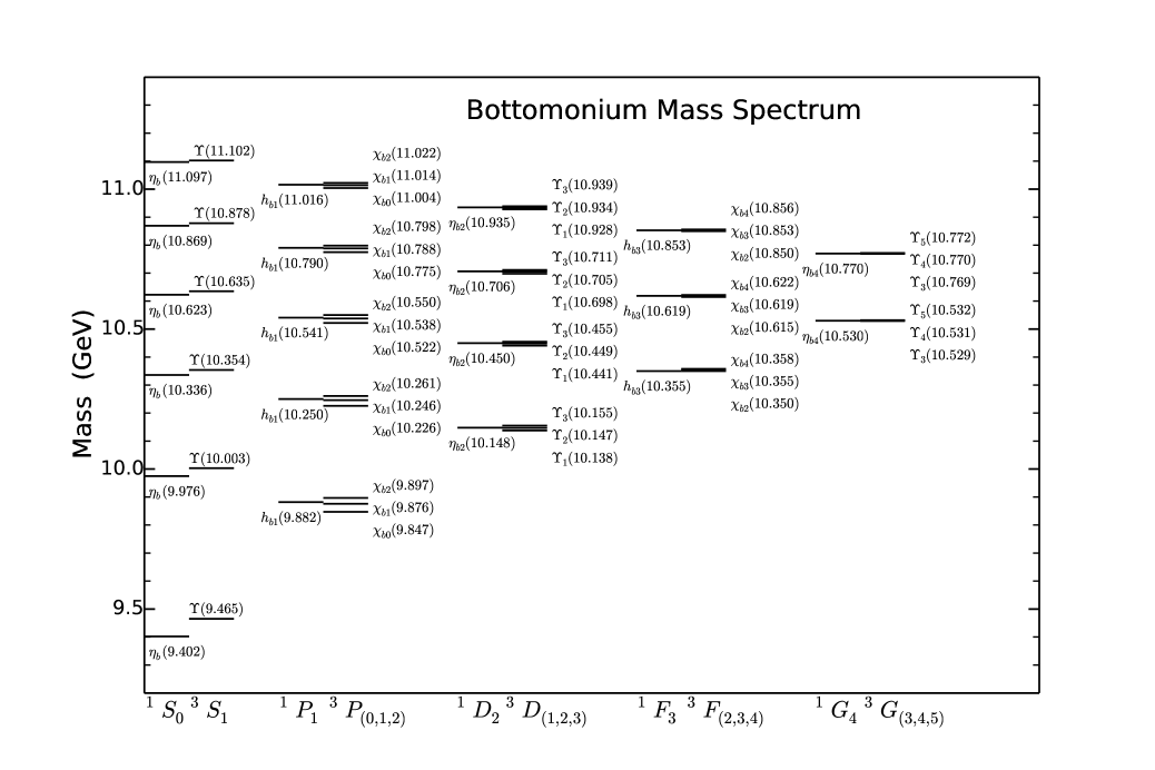
Figure 1: The $b\bar{b}$ mass spectrum as predicted by the relativized quark model godfrey85xj .

Table 1: Masses and effective harmonic oscillator parameter values ($\beta$) for $S$-, $P$- and $D$-wave Bottomonium mesons.

Meson	$M_{theo}$ (MeV)	$M_{exp}$ (MeV)	$\beta$ (GeV)
$\Upsilon(1^{3}S_{1})$	9465	$9460.30\pm 0.26$	1.157
$\eta_{b}(1^{1}S_{0})$	9402	$9398.0\pm 3.2$	1.269
$\Upsilon(2^{3}S_{1})$	10003	$10023.26\pm 0.31$	0.819
$\eta_{b}(2^{1}S_{0})$	9976	$9999.0\pm 3.5^{+2.8}_{-1.9}$	0.854
$\Upsilon(3^{3}S_{1})$	10354	$10355.2\pm 0.5$	0.698
$\eta_{b}(3^{1}S_{0})$	10336	10337	0.719
$\Upsilon(4^{3}S_{1})$	10635	$10579.4\pm 1.2$	0.638
$\eta_{b}(4^{1}S_{0})$	10623	10567	0.654
$\Upsilon(5^{3}S_{1})$	10878	$10876\pm 11$	0.600
$\eta_{b}(5^{1}S_{0})$	10869	10867	0.615
$\Upsilon(6^{3}S_{1})$	11102	$11019\pm 8$	0.578
$\eta_{b}(6^{1}S_{0})$	11097	11014	0.593
$\chi_{b2}(1^{3}P_{2})$	9897	$9912.21\pm 0.26\pm 0.31$	0.858
$\chi_{b1}(1^{3}P_{1})$	9876	$9892.78\pm 0.26\pm 0.31$	0.889
$\chi_{b0}(1^{3}P_{0})$	9847	$9859.44\pm 0.42\pm 0.31$	0.932
$h_{b}(1^{1}P_{1})$	9882	$9899.3\pm 1.0$	0.880
$\chi_{b2}(2^{3}P_{2})$	10261	$10268.65\pm 0.22\pm 0.50$	0.711
$\chi_{b1}(2^{3}P_{1})$	10246	$10255.46\pm 0.22\pm 0.50$	0.725
$\chi_{b0}(2^{3}P_{0})$	10226	$10232.5\pm 0.4\pm 0.5$	0.742
$h_{b}(2^{1}P_{1})$	10250	$10259.8\pm 0.5\pm 1.1$	0.721
$\chi_{b2}(3^{3}P_{2})$	10550	10528	0.640
$\chi_{b1}(3^{3}P_{1})$	10538	$10515.7^{+2.2+1.5}_{-3.9-2.1}$	0.649
$\chi_{b0}(3^{3}P_{0})$	10522	10500	0.660
$h_{b}(3^{1}P_{1})$	10541	10519	0.649
$\chi_{b2}(4^{3}P_{2})$	10798	N/A	0.598
$\chi_{b1}(4^{3}P_{1})$	10788	N/A	0.605
$\chi_{b0}(4^{3}P_{0})$	10775	N/A	0.613
$h_{b}(4^{1}P_{1})$	10790	N/A	0.603
$\chi_{b2}(5^{3}P_{2})$	11022	N/A	0.570
$\chi_{b1}(5^{3}P_{1})$	11014	N/A	0.576
$\chi_{b0}(5^{3}P_{0})$	11004	N/A	0.585
$h_{b}(5^{1}P_{1})$	11016	N/A	0.575
$\Upsilon_{3}(1^{3}D_{3})$	10155	10172	0.752
$\Upsilon_{2}(1^{3}D_{2})$	10147	$10163.7\pm 1.4$	0.763
$\Upsilon_{1}(1^{3}D_{1})$	10138	10155	0.776
$\eta_{b2}(1^{1}D_{2})$	10148	10165	0.761
$\Upsilon_{3}(2^{3}D_{3})$	10455	N/A	0.660
$\Upsilon_{2}(2^{3}D_{2})$	10449	N/A	0.666
$\Upsilon_{1}(2^{3}D_{1})$	10441	N/A	0.672
$\eta_{b2}(2^{1}D_{2})$	10450	N/A	0.665
$\Upsilon_{3}(3^{3}D_{3})$	10711	N/A	0.609
$\Upsilon_{2}(3^{3}D_{2})$	10705	N/A	0.613
$\Upsilon_{1}(3^{3}D_{1})$	10698	N/A	0.618
$\eta_{b2}(3^{1}D_{2})$	10706	N/A	0.612
$\Upsilon_{3}(4^{3}D_{3})$	10939	N/A	0.577
$\Upsilon_{2}(4^{3}D_{2})$	10934	N/A	0.580
$\Upsilon_{1}(4^{3}D_{1})$	10928	N/A	0.583
$\eta_{b2}(4^{1}D_{2})$	10935	N/A	0.579

Table 2: Masses and effective harmonic oscillator parameter values ($\beta$) for $F$- and $G$-wave Bottomonium mesons.

Meson	$M_{theo}$ (MeV)	$M_{exp}$ (MeV)	$\beta$ (GeV)
$\chi_{b4}(1^{3}F_{4})$	10358	N/A	0.693
$\chi_{b3}(1^{3}F_{3})$	10355	N/A	0.698
$\chi_{b2}(1^{3}F_{2})$	10350	N/A	0.704
$h_{b3}(1^{1}F_{3})$	10355	N/A	0.698
$\chi_{b4}(2^{3}F_{4})$	10622	N/A	0.626
$\chi_{b3}(2^{3}F_{3})$	10619	N/A	0.630
$\chi_{b2}(2^{3}F_{2})$	10615	N/A	0.633
$h_{b3}(2^{1}F_{3})$	10619	N/A	0.629
$\chi_{b4}(3^{3}F_{4})$	10856	N/A	0.587
$\chi_{b3}(3^{3}F_{3})$	10853	N/A	0.590
$\chi_{b2}(3^{3}F_{2})$	10850	N/A	0.592
$h_{b3}(3^{1}F_{3})$	10853	N/A	0.589
$\Upsilon_{5}(1^{3}G_{5})$	10532	N/A	0.653
$\Upsilon_{4}(1^{3}G_{4})$	10531	N/A	0.656
$\Upsilon_{3}(1^{3}G_{3})$	10529	N/A	0.660
$\eta_{b4}(1^{1}G_{4})$	10530	N/A	0.656
$\Upsilon_{5}(2^{3}G_{5})$	10772	N/A	0.602
$\Upsilon_{4}(2^{3}G_{4})$	10770	N/A	0.604
$\Upsilon_{3}(2^{3}G_{3})$	10769	N/A	0.606
$\eta_{b4}(2^{1}G_{4})$	10770	N/A	0.604

Table 3: Masses and effective $\beta$ values for $B$ mesons used in the calculations of bottomonium strong decay widths. The physical $1P_{1}^{\prime}$ and $1P_{1}$ states are mixtures of $1^{1}P_{1}$ and $1^{3}P_{1}$ with singlet-triplet mixing angle $\theta_{1P}=-30.3^{\circ}$ for $b\bar{q}$ ordering. Where two values of $\beta$ are listed, the first (second) value is for the singlet (triplet) state.

Meson	State	$M_{theo}$ (MeV)	$M_{exp}$ (MeV)	$\beta$ (GeV)
$B^{\pm}$	$1^{1}S_{0}$	5312	$5279.26\pm 0.17$	0.580
$B^{0}$	$1^{1}S_{0}$	5312	$5279.58\pm 0.17$	0.580
$B^{*}$	$1^{3}S_{1}$	5371	$5325.2\pm 0.4$	0.542
$B(1^{3}P_{0})$	$1^{3}P_{0}$	5756	5702	0.536
$B(1P_{1})$	$\cos\theta_{1P}(1^{1}P_{1})+\sin\theta_{1P}(1^{3}P_{1})$	5777	$5723.5\pm 2.0$	0.499, 0.511
$B(1P_{1}^{\prime})$	$-\sin\theta_{1P}(1^{1}P_{1})+\cos\theta_{1P}(1^{3}P_{1})$	5784	5730	0.499, 0.511
$B(1^{3}P_{2})$	$1^{3}P_{2}$	5797	$5743\pm 5$	0.472
$B_{s}$	$1^{1}S_{0}$	5394	$5366.77\pm 0.24$	0.636
$B_{s}^{*}$	$1^{3}S_{1}$	5450	$5415.4^{+2.4}_{-2.1}$	0.595

Table 4: Partial widths and branching ratios for strong and electromagnetic decays and transitions for the $1S$ and $2S$ bottomonium states. The state’s mass is given in GeV and is listed below the state’s name in column 1. Column 4, labelled $\cal M$ gives the matrix element appropriate to the particular decay; for $S$-wave annihilation decays ${\cal M}$ designates $\Psi(0)=R(0)/\sqrt{4\pi}$ representing the wavefunction at the origin and for radiative transitions the E1 or M1 matrix elements are $\langle\psi_{f}|r|\psi_{i}\rangle$ (GeV^-1) and $\langle\psi_{f}|j_{0}(kr/2)|\psi_{i}\rangle$ respectively. Details of the calculations are given in the text.

Initial www	Final	$M_{f}$	$\cal M$	Predicted		Measured
state	state	(GeV)		Width (keV)	BR (%)	Width (keV)	BR (%)
$\Upsilon(1^{3}S_{1})$	$\ell^{+}\ell^{-}$		$0.793$	1.44	2.71	$1.34\pm 0.04$	$2.48\pm 0.05$
9.460	$ggg$		$0.793$	47.6	89.6	$44.1\pm 1.1$	$81.7\pm 0.7$
	$\gamma gg$		$0.793$	1.2	2.3	$1.2\pm 0.3$	$2.2\pm 0.6$
	$\gamma\gamma\gamma$		$0.793$	$1.7\times 10^{-5}$	$3.2\times 10^{-5}$
	$\eta_{b}(1^{1}S_{0})\gamma$	9.398	$0.9947$	$0.010$	0.019
	Total			53.1	100	$54.02\pm 1.25$
$\eta_{b}(1^{1}S_{0})$	$gg$		$1.081$	16.6 MeV	$\sim 100$
9.398	$\gamma\gamma$		$1.081$	0.94	0.0057
	Total			16.6 MeV	100	$10.8^{+6.0}_{-4.2}$ MeV
$\Upsilon(2^{3}S_{1})$	$\ell^{+}\ell^{-}$		$0.597$	0.73	1.8	$0.62\pm 0.06$	$1.93\pm 0.17$
10.023	$ggg$		$0.597$	26.3	65.4	$18.8\pm 1.6$	$58.8\pm 1.2$
	$\gamma gg$		$0.597$	0.68	1.7	$2.81\pm 0.42$	$8.8\pm 1.1$
	$\gamma\gamma\gamma$		$0.597$	$9.8\times 10^{-6}$	$2.4\times 10^{-5}$
	$\chi_{b2}(1^{3}P_{2})\gamma$	9.912	$-1.524$	1.88	4.67	$2.29\pm 0.22$	$7.15\pm 0.35$
	$\chi_{b1}(1^{3}P_{1})\gamma$	9.893	$-1.440$	1.63	4.05	$2.21\pm 0.22$	$6.9\pm 0.4$
	$\chi_{b0}(1^{3}P_{0})\gamma$	9.859	$-1.330$	0.91	2.3	$1.22\pm 0.16$	$3.8\pm 0.4$
	$\eta_{b}(2^{1}S_{0})\gamma$	9.999	$0.9924$	$5.9\times 10^{-4}$	$1.5\times 10^{-3}$
	$\eta_{b}(1^{1}S_{0})\gamma$	9.398	$0.0913$	0.081	0.20	$0.012\pm 0.004$	$(3.9\pm 1.5)\times 10^{-2}$
	$\Upsilon(1^{3}S_{1})\pi\pi$			8.46	21.0	$8.46\pm 0.71$	$26.45\pm 0.48$
	Total			40.2	100	$31.98\pm 2.63$
$\eta_{b}(2^{1}S_{0})$	$gg$		$0.718$	7.2 MeV	$\sim 100$
9.999	$\gamma\gamma$		$0.718$	0.41	$5.7\times 10^{-3}$
	$h_{b}(1^{1}P_{1})\gamma$	9.899	$-1.526$	2.48	0.034
	$\Upsilon(1^{3}S_{1})\gamma$	9.460	$-0.0610$	0.068	$9.4\times 10^{-4}$
	$\eta_{b}(1^{1}S_{0})\pi\pi$			12.4	0.17
	Total			7.2 MeV	100	$<24$ MeV

Table 5: Partial widths and branching ratios for strong and electromagnetic decays and transitions for the $3S$ states. See the caption to Table 4 for further details.

Initial www	Final	$M_{f}$	$\cal M$	Predicted		Measured
state	state	(GeV)		Width (keV)	BR (%)	Width (keV)	BR (%)
$\Upsilon(3^{3}S_{1})$	$\ell^{+}\ell^{-}$		$0.523$	0.53	1.8	$0.44\pm 0.06$	$2.18\pm 0.21$
10.355	$ggg$		$0.523$	19.8	67.9	$7.25\pm 0.84$	$35.7\pm 2.6$
	$\gamma gg$		$0.523$	0.52	1.8	$0.20\pm 0.04$	$0.97\pm 0.18$
	$\gamma\gamma\gamma$		$0.523$	$7.6\times 10^{-6}$	$2.6\times 10^{-5}$
	$\chi_{b2}(2^{3}P_{2})\gamma$	10.269	$-2.446$	2.30	7.90	$2.66\pm 0.40$	$13.1\pm 1.6$
	$\chi_{b1}(2^{3}P_{1})\gamma$	10.255	$-2.326$	1.91	6.56	$2.56\pm 0.34$	$12.6\pm 1.2$
	$\chi_{b0}(2^{3}P_{0})\gamma$	10.232	$-2.169$	1.03	3.54	$1.20\pm 0.16$	$5.9\pm 0.6$
	$\chi_{b2}(1^{3}P_{2})\gamma$	9.912	$0.096$	0.45	1.5	$0.20\pm 0.03$	$0.99\pm 0.13$
	$\chi_{b1}(1^{3}P_{1})\gamma$	9.893	$0.039$	0.05	0.2	$0.018\pm 0.010$	$0.09\pm 0.05$
	$\chi_{b0}(1^{3}P_{0})\gamma$	9.859	$-0.028$	0.01	0.03	$0.055\pm 0.010$	$0.27\pm 0.04$
	$\eta_{b}(3^{1}S_{0})\gamma$	10.337	$0.9920$	$2.5\times 10^{-4}$	$8.6\times 10^{-4}$
	$\eta_{b}(2^{1}S_{0})\gamma$	9.999	$0.1003$	0.19	0.65	$<0.12$	$<0.062$ at 90% C.L.
	$\eta_{b}(1^{1}S_{0})\gamma$	9.398	$0.0427$	0.060	0.20	$0.01\pm 0.002$	$0.051\pm 0.007$
	$\Upsilon(1^{3}S_{1})\pi\pi$			1.34	4.60	$1.335\pm 0.125$	$6.57\pm 0.15$
	$\Upsilon(2^{3}S_{1})\pi\pi$			0.95	3.3	$0.949\pm 0.098$	$4.67\pm 0.23$
	Total			29.1	100	$20.32\pm 1.85$
$\eta_{b}(3^{1}S_{0})$	$gg$		$0.601$	4.9 MeV	$\sim 100$
10.337	$\gamma\gamma$		$0.601$	0.29	$5.9\times 10^{-3}$
	$h_{b}(2^{1}P_{1})\gamma$	10.260	$-2.461$	2.96	0.060
	$h_{b}(1^{1}P_{1})\gamma$	9.899	$0.1235$	1.3	0.026
	$\Upsilon(2^{3}S_{1})\gamma$	10.023	$-0.0484$	$9.1\times 10^{-3}$	$1.8\times 10^{-4}$
	$\Upsilon(1^{3}S_{1})\gamma$	9.460	$-0.031$	$0.074$	$1.5\times 10^{-3}$
	$\eta_{b}(1^{1}S_{0})\pi\pi$			$1.70\pm 0.12$	$3.5\times 10^{-2}$
	$\eta_{b}(2^{1}S_{0})\pi\pi$			$1.16\pm 0.10$	$2.4\times 10^{-2}$
	Total			4.9 MeV	100

Table 6: Partial widths and branching ratios for strong and electromagnetic decays and transitions and OZI allowed strong decays for the $4S$ and $5S$ bottomonium states. Details of the OZI allowed decay amplitudes are described in the appendix. See the caption to Table 4 for further details.

Initial www	Final	$M_{f}$	$\cal M$	Predicted		Measured
state	state	(GeV)		Width (keV)	BR (%)	Width (keV)	BR (%)
$\Upsilon(4^{3}S_{1})$	$\ell^{+}\ell^{-}$		$0.459$	0.39	$1.8\times 10^{-3}$	$0.32\pm 0.04$	$(1.57\pm 0.08)\times 10^{-3}$
10.579	$ggg$		$0.459$	15.1	0.0686
	$\gamma gg$		$0.459$	0.40	$1.8\times 10^{-3}$
	$\gamma\gamma\gamma$		$0.459$	$6.0\times 10^{-6}$	$2.7\times 10^{-8}$
	$\chi_{b2}(3^{3}P_{2})\gamma$	10.528	$-3.223$	0.82	$3.7\times 10^{-3}$
	$\chi_{b1}(3^{3}P_{1})\gamma$	10.516	$-3.072$	0.84	$3.8\times 10^{-3}$
	$\chi_{b0}(3^{3}P_{0})\gamma$	10.500	$-2.869$	0.48	$2.2\times 10^{-3}$
	$\Upsilon(1^{3}S_{1})\pi^{+}\pi^{-}$			1.66	$7.54\times 10^{-3}$	$1.66\pm 0.24$	$(8.1\pm 0.6)\times 10^{-3}$
	$\Upsilon(2^{3}S_{1})\pi^{+}\pi^{-}$			1.76	$8.00\times 10^{-3}$	$1.76\pm 0.34$	$(8.6\pm 1.3)\times 10^{-3}$
	$BB$			22.0 MeV	$\sim 100$		$>96$ at 95% C.L.
	Total			22.0 MeV	100	$20.5\pm 2.5$ MeV
$\eta_{b}(4^{1}S_{0})$	$gg$		$0.500$	3.4 MeV	$\sim 100$
10.567	$\gamma\gamma$		$0.500$	0.20	$5.9\times 10^{-3}$
	$h_{b}(3^{1}P_{1})\gamma$	10.519	$-3.238$	1.24	$3.6\times 10^{-2}$
	$\eta_{b}(1^{1}S_{0})\pi^{+}\pi^{-}$			$2.03\pm 0.29$	$6.0\times 10^{-2}$
	$\eta_{b}(2^{1}S_{0})\pi^{+}\pi^{-}$			$1.90\pm 0.36$	$5.6\times 10^{-2}$
	Total			3.4 MeV	100
$\Upsilon(5^{3}S_{1})$	$\ell^{+}\ell^{-}$		$0.432$	0.33	$1.2\times 10^{-3}$	$0.31\pm 0.23$	$(5.6\pm 3.1)\times 10^{-4}$
10.876	$ggg$		$0.432$	13.1	$4.78\times 10^{-2}$
	$\chi_{b2}(4^{3}P_{2})\gamma$	10.798	$-3.908$	4.3	$1.6\times 10^{-2}$
	$\chi_{b1}(4^{3}P_{1})\gamma$	10.788	$-3.724$	3.4	$1.2\times 10^{-2}$
	$\chi_{b0}(4^{3}P_{0})\gamma$	10.775	$-3.483$	1.5	$5.5\times 10^{-3}$
	$\chi_{b2}(3^{3}P_{2})\gamma$	10.528	$0.131$	0.42	$1.5\times 10^{-3}$
	$\chi_{b1}(3^{3}P_{1})\gamma$	10.516	$0.0020$	$6.2\times 10^{-5}$	$2.3\times 10^{-7}$
	$\chi_{b0}(3^{3}P_{0})\gamma$	10.500	$-0.156$	0.15	$5.5\times 10^{-4}$
	$BB$			5.35 MeV	19.5	$3.0\pm 1.6$ MeV	$5.5\pm 1.0$
	$BB^{*}$			16.6 MeV	60.6	$7.5\pm 3.9$ MeV	$13.7\pm 1.6$
	$B^{*}B^{*}$			2.42 MeV	8.83	$21\pm 11$ MeV	$38.1\pm 3.4$
	$B_{s}B_{s}$			0.157 MeV	0.573	$0.3\pm 0.3$ MeV	$0.5\pm 0.5$
	$B_{s}B_{s}^{*}$			0.833 MeV	3.04	$0.74\pm 0.42$ MeV	$1.35\pm 0.32$
	$B_{s}^{*}B_{s}^{*}$			2.00 MeV	7.30	$9.7\pm 5.1$ MeV	$17.6\pm 2.7$
	Total			27.4 MeV	100	$55\pm 28$ MeV
$\eta_{b}(5^{1}S_{0})$	$gg$		$0.464$	2.9 MeV	13
10.867	$\gamma\gamma$		$0.464$	0.17	$7.4\times 10^{-4}$
	$h_{b}(4^{1}P_{1})\gamma$	10.790	$3.925$	7.5	$3.3\times 10^{-2}$
	$h_{b}(3^{1}P_{1})\gamma$	10.519	$0.162$	1.1	$4.8\times 10^{-3}$
	$BB^{*}$			13.1 MeV	57.0
	$B^{*}B^{*}$			0.914 MeV	3.97
	$B_{s}B_{s}^{*}$			0.559 MeV	2.43
	$B_{s}^{*}B_{s}^{*}$			5.49 MeV	23.9
	Total			23.0 MeV	100

as appropriate.

Table 7: Partial widths and branching ratios for strong and electromagnetic decays and transitions and OZI allowed strong decays for the $6S$ states. Details of the OZI allowed decay amplitudes are described in the appendix. See the caption to Table 4 for further details.

Initial www	Final	$M_{f}$	$\cal M$	Predicted		Measured
state	state			Width (keV)	BR (%)	Width (keV)	BR (%)
$\Upsilon(6^{3}S_{1})$	$\ell^{+}\ell^{-}$		$0.396$	0.27	$8.0\times 10^{-4}$	$0.13\pm 0.05$	$(1.6\pm 0.5)\times 10^{-4}$
11.019	$ggg$		$0.396$	11.0	0.0324
	$\chi_{b2}(5^{3}P_{2})\gamma$	11.022		below threshold	-
	$\chi_{b1}(5^{3}P_{1})\gamma$	11.014	$-4.282$	$8.3\times 10^{-4}$	$2.4\times 10^{-6}$
	$\chi_{b0}(5^{3}P_{0})\gamma$	11.004	$-3.992$	$6.4\times 10^{-3}$	$1.9\times 10^{-5}$
	$\chi_{b2}(4^{3}P_{2})\gamma$	10.798	$0.116$	$8.5\times 10^{-2}$	$2.5\times 10^{-4}$
	$\chi_{b1}(4^{3}P_{1})\gamma$	10.788	$-0.054$	0.012	$3.5\times 10^{-5}$
	$\chi_{b0}(4^{3}P_{0})\gamma$	10.775	$-0.244$	0.1	$3\times 10^{-4}$
	$\chi_{b2}(3^{3}P_{2})\gamma$	10.528	$0.089$	0.53	$1.6\times 10^{-3}$
	$\chi_{b1}(3^{3}P_{1})\gamma$	10.516	$0.100$	0.43	$1.3\times 10^{-3}$
	$\chi_{b0}(3^{3}P_{0})\gamma$	10.500	$0.115$	0.21	$6.2\times 10^{-4}$
	$BB$			1.32 MeV	3.89
	$BB^{*}$			7.59 MeV	22.4
	$BB(1P_{1})$			7.81 MeV	23.0
	$BB(1P_{1}^{\prime})$			10.8 MeV	31.8
	$B^{*}B^{*}$			5.89 MeV	17.4
	$B_{s}B_{s}$			1.31	$3.86\times 10^{-3}$
	$B_{s}B_{s}^{*}$			0.136 MeV	0.401
	$B_{s}^{*}B_{s}^{*}$			0.310 MeV	0.914
	Total			33.9 MeV	100	$79\pm 16$ MeV
$\eta_{b}(6^{1}S_{0})$	$gg$		$0.410$	2.2 MeV	16
11.014	$\gamma\gamma$		$0.410$	0.14	$1.0\times 10^{-3}$
	$h_{b}(5^{1}P_{1})\gamma$	11.016		below threshold	-
	$h_{b}(4^{1}P_{1})\gamma$	10.790	$0.136$	0.22	$1.6\times 10^{-3}$
	$h_{b}(3^{1}P_{1})\gamma$	10.519	$0.123$	1.8	$1.3\times 10^{-2}$
	$BB^{*}$			8.98 MeV	66.0
	$BB(1^{3}P_{0})$			0.745 MeV	5.48
	$B^{*}B^{*}$			1.14 MeV	8.38
	$B_{s}B_{s}^{*}$			0.420 MeV	3.09
	$B_{s}^{*}B_{s}^{*}$			0.156 MeV	1.15
	Total			13.6 MeV	100

Table 8: Partial widths and branching ratios for strong and electromagnetic decays and transitions for the $1P$ states. For $P$-wave annihilation decays ${\cal M}$ designates $R^{\prime}(0)$, the first derivative of the radial wavefunction at the origin. See the caption to Table 4 for further details.

Initial www	Final	$M_{f}$	$\cal M$	Predicted		Measured
state	state	(GeV)		Width (keV)	BR (%)	BR (%)
$\chi_{b2}(1^{3}P_{2})$	$gg$		$1.318$	147	81.7
9.912	$\gamma\gamma$		$1.318$	$9.3\times 10^{-3}$	$5.2\times 10^{-3}$
	$\Upsilon(1^{3}S_{1})\gamma$	9.460	$1.028$	32.8	18.2	$19.1\pm 1.2$
	$h_{b}(1^{1}P_{1})\gamma$	9.899	$1.000$	$9.6\times 10^{-5}$	$5.3\times 10^{-5}$
	Total			180.	100
$\chi_{b1}(1^{3}P_{1})$	$q\bar{q}+g$		$1.700$	67	70.
9.893	$\Upsilon(1^{3}S_{1})\gamma$	9.460	$1.040$	29.5	31	$33.9\pm 2.2$
	Total			96	100
$\chi_{b0}(1^{3}P_{0})$	$gg$		$2.255$	2.6 MeV	$\sim 100$
9.859	$\gamma\gamma$		$2.255$	0.15	$5.8\times 10^{-3}$
	$\Upsilon(1^{3}S_{1})\gamma$	9.460	$1.050$	23.8	0.92	$1.76\pm 0.35$
	Total			2.6 MeV	100
$h_{b}(1^{1}P_{1})$	$ggg$		$1.583$	37	51
9.899	$\eta_{b}(1^{1}S_{0})\gamma$	9.398	$0.922$	35.7	49	$49^{+8}_{-7}$
	$\chi_{b1}(1^{3}P_{1})\gamma$	9.893	$1.000$	$1.0\times 10^{-5}$	$1.4\times 10^{-5}$
	$\chi_{b0}(1^{3}P_{0})\gamma$	9.859	$0.998$	$8.9\times 10^{-4}$	$1.2\times 10^{-5}$
	Total			73	100

Table 9: Partial widths and branching ratios for strong and electromagnetic decays and transitions for the $2P$ states. For $P$-wave annihilation decays ${\cal M}$ designates $R^{\prime}(0)$, the first derivative of the radial wavefunction at the origin. See the caption to Table 4 for further details.

Initial www	Final	$M_{f}$	$\cal M$	Predicted		Measured
state	state	(GeV)		Width (keV)	BR (%)	BR (%)
$\chi_{b2}(2^{3}P_{2})$	$gg$		$1.528$	207	89.0
10.269	$\gamma\gamma$		$1.528$	$1.2\times 10^{-2}$	$5.2\times 10^{-3}$
	$\Upsilon(2^{3}S_{1})\gamma$	10.023	$1.667$	14.3	6.15	$10.6\pm 2.6$
	$\Upsilon(1^{3}S_{1})\gamma$	9.460	$0.224$	8.4	3.6	$7.0\pm 0.7$
	$\Upsilon_{3}(1^{3}D_{3})\gamma$	10.172	$-1.684$	1.5	0.65
	$\Upsilon_{2}(1^{3}D_{2})\gamma$	10.164	$-1.625$	0.3	0.1
	$\Upsilon_{1}(1^{3}D_{1})\gamma$	10.154	$-1.561$	0.03	0.01
	$h_{b}(2^{1}P_{1})\gamma$	10.260	$1.000$	$2.8\times 10^{-5}$	$1.2\times 10^{-5}$
	$h_{b}(1^{1}P_{1})\gamma$	9.899	$-0.011$	$2.4\times 10^{-4}$	$1.0\times 10^{-4}$
	$\chi_{b2}(1^{3}P_{2})\pi\pi$			$0.62\pm 0.12$	0.27	$0.51\pm 0.09$
	$\chi_{b1}(1^{3}P_{1})\pi\pi$			0.23	0.10
	$\chi_{b0}(1^{3}P_{0})\pi\pi$			0.10	0.043
	Total			232.5	100
$\chi_{b1}(2^{3}P_{1})$	$q\bar{q}+g$		$1.857$	96	82
10.255	$\Upsilon(2^{3}S_{1})\gamma$	10.023	$1.749$	13.3	11.3	$19.9\pm 1.9$
	$\Upsilon(1^{3}S_{1})\gamma$	9.460	$0.184$	5.5	4.7	$9.2\pm 0.8$
	$\Upsilon_{2}(1^{3}D_{2})\gamma$	10.164	$-1.701$	1.2	1.0
	$\Upsilon_{1}(1^{3}D_{1})\gamma$	10.154	$-1.639$	0.5	0.4
	$h_{b}(1^{1}P_{1})\gamma$	9.899	$-0.035$	$2.2\times 10^{-3}$	$1.9\times 10^{-3}$
	$\chi_{b2}(1^{3}P_{2})\pi\pi$			0.38	0.32
	$\chi_{b1}(1^{3}P_{1})\pi\pi$			$0.57\pm 0.09$	0.48	$0.91\pm 0.13$
	$\chi_{b0}(1^{3}P_{0})\pi\pi$			$\sim 0$	$\sim 0$
	Total			117	100
$\chi_{b0}(2^{3}P_{0})$	$gg$		$2.290$	2.6 MeV	$\sim 100$
10.232	$\gamma\gamma$		$2.290$	0.15	$5.7\times 10^{-3}$
	$\Upsilon(2^{3}S_{1})\gamma$	10.023	$1.842$	10.9	0.42	$4.6\pm 2.1$
	$\Upsilon(1^{3}S_{1})\gamma$	9.460	$0.130$	2.5	$9.6\times 10^{-2}$	$0.9\pm 0.6$
	$\Upsilon_{1}(1^{3}D_{1})\gamma$	10.154	$-1.731$	1.0	$3.8\times 10^{-2}$
	$h_{b}(1^{1}P_{1})\gamma$	9.899	$-0.079$	$9.7\times 10^{-3}$	$3.7\times 10^{-4}$
	$\chi_{b2}(1^{3}P_{2})\pi\pi$			0.5	$2\times 10^{-2}$
	$\chi_{b1}(1^{3}P_{1})\pi\pi$			$\sim 0$	$\sim 0$
	$\chi_{b0}(1^{3}P_{0})\pi\pi$			0.44	$1.7\times 10^{-2}$
	Total			2.6 MeV	100
$h_{b}(2^{1}P_{1})$	$ggg$		$1.758$	54	64
10.260	$\eta_{b}(2^{1}S_{0})\gamma$	9.999	$1.510$	14.1	17	$48\pm 13$
	$\eta_{b}(1^{1}S_{0})\gamma$	9.398	$0.252$	13.0	15	$22\pm 5$
	$\eta_{b2}(1^{1}D_{2})\gamma$	10.165	$-1.689$	1.7	2.0
	$\chi_{b2}(1^{3}P_{2})\gamma$	9.912	$-0.027$	$2.2\times 10^{-3}$	$2.6\times 10^{-3}$
	$\chi_{b1}(1^{3}P_{1})\gamma$	9.893	$-0.023$	$1.1\times 10^{-3}$	$1.3\times 10^{-3}$
	$\chi_{b0}(1^{3}P_{0})\gamma$	9.859	$0.019$	$3.2\times 10^{-4}$	$3.8\times 10^{-4}$
	$h_{b}(1^{1}P_{1})\pi\pi$			0.94	1.1
	Total			84	100

Table 10: Partial widths and branching ratios for strong and electromagnetic decays and transitions for the $3P$ states. For $P$-wave annihilation decays ${\cal M}$ designates $R^{\prime}(0)$, the first derivative of the radial wavefunction at the origin. See the caption to Table 4 for further details.

Initial www	Final	$M_{f}$	$\cal M$	Width	BR
state	state	(GeV)		(keV)	(%)
$\chi_{b2}(3^{3}P_{2})$	$gg$		$1.584$	227	91.9
10.528	$\gamma\gamma$		$1.584$	$1.3\times 10^{-2}$	$5.3\times 10^{-3}$
	$\Upsilon(3^{3}S_{1})\gamma$	10.355	$2.255$	9.3	3.8
	$\Upsilon(2^{3}S_{1})\gamma$	10.023	$0.323$	4.5	1.8
	$\Upsilon(1^{3}S_{1})\gamma$	9.460	$0.086$	2.8	1.1
	$\Upsilon_{3}(2^{3}D_{3})\gamma$	10.455	$-2.568$	1.5	0.61
	$\Upsilon_{2}(2^{3}D_{2})\gamma$	10.449	$-2.482$	0.32	0.13
	$\Upsilon_{1}(2^{3}D_{1})\gamma$	10.441	$-2.389$	0.027	0.011
	$\Upsilon_{3}(1^{3}D_{3})\gamma$	10.172	$0.042$	0.046	0.019
	$\chi_{b2}(1^{3}P_{2})\pi\pi$			0.68	0.28
	$\chi_{b1}(1^{3}P_{1})\pi\pi$			0.52	0.21
	$\chi_{b0}(1^{3}P_{0})\pi\pi$			0.24	0.10
	Total			247	100
$\chi_{b1}(3^{3}P_{1})$	$q\bar{q}+g$		$1.814$	101	86.3
10.516	$\Upsilon(3^{3}S_{1})\gamma$	10.355	$2.388$	8.4	7.2
	$\Upsilon(2^{3}S_{1})\gamma$	10.023	$0.278$	3.1	2.6
	$\Upsilon(1^{3}S_{1})\gamma$	9.460	$0.061$	1.3	1.1
	$\Upsilon_{2}(2^{3}D_{2})\gamma$	10.449	$-2.595$	1.1	0.94
	$\Upsilon_{1}(2^{3}D_{1})\gamma$	10.441	$-2.506$	0.47	0.40
	$\Upsilon_{2}(1^{3}D_{2})\gamma$	10.164	$0.060$	0.080	0.068
	$\Upsilon_{1}(1^{3}D_{1})\gamma$	10.154	$0.029$	$7.0\times 10^{-3}$	$6.0\times 10^{-3}$
	$\chi_{b2}(1^{3}P_{2})\pi\pi$			0.88	0.75
	$\chi_{b1}(1^{3}P_{1})\pi\pi$			0.56	0.48
	$\chi_{b0}(1^{3}P_{0})\pi\pi$			$\sim 0$	$\sim 0$
	Total			117	100
$\chi_{b0}(3^{3}P_{0})$	$gg$		$2.104$	2.2 MeV	$\sim$100
10.500	$\gamma\gamma$		$2.104$	0.13	$5.9\times 10^{-3}$
	$\Upsilon(3^{3}S_{1})\gamma$	10.355	$2.537$	6.9	0.31
	$\Upsilon(2^{3}S_{1})\gamma$	10.023	$0.213$	1.7	0.077
	$\Upsilon(1^{3}S_{1})\gamma$	9.460	$0.029$	0.3	0.01
	$\Upsilon_{1}(2^{3}D_{1})\gamma$	10.441	$-2.637$	1.0	0.045
	$\Upsilon_{1}(1^{3}D_{1})\gamma$	10.154	$0.084$	0.20	0.0091
	$\chi_{b2}(1^{3}P_{2})\pi\pi$			1.2	0.054
	$\chi_{b1}(1^{3}P_{1})\pi\pi$			$\sim 0$	$\sim 0$
	$\chi_{b0}(1^{3}P_{0})\pi\pi$			0.27	0.012
	Total			2.2 MeV	100
$h_{b}(3^{1}P_{1})$	$ggg$		$1.749$	59	71
10.519	$\eta_{b}(3^{1}S_{0})\gamma$	10.337	$2.047$	8.9	11
	$\eta_{b}(2^{1}S_{0})\gamma$	9.999	$0.418$	8.2	9.9
	$\eta_{b}(1^{1}S_{0})\gamma$	9.398	$0.091$	3.6	4.3
	$\eta_{b2}(2^{1}D_{2})\gamma$	10.450	$-2.579$	1.6	1.9
	$\eta_{b2}(1^{1}D_{2})\gamma$	10.165	$0.052$	0.081	0.098
	$\chi_{b2}(1^{3}P_{2})\gamma$	9.912	$-0.032$	$1.4\times 10^{-2}$	$1.7\times 10^{-2}$
	$\chi_{b1}(1^{3}P_{1})\gamma$	9.893	$-0.031$	$9.3\times 10^{-3}$	$1.1\times 10^{-2}$
	$\chi_{b0}(1^{3}P_{0})\gamma$	9.859	$-0.016$	$9.8\times 10^{-4}$	$1.2\times 10^{-3}$
	$h_{b}(1^{1}P_{1})\pi\pi$			1.4	1.7
	Total			83	100

Table 11: Partial widths and branching ratios for strong and electromagnetic decays and transitions and OZI allowed strong decays for the $4P$ states. For $P$-wave annihilation decays ${\cal M}$ designates $R^{\prime}(0)$, the first derivative of the radial wavefunction at the origin. Details of the OZI allowed decay amplitudes are described in the appendix. See the caption to Table 4 for further details.

Initial www	Final	$M_{f}$	$\cal M$	Width	BR
state	state	(GeV)		(keV)	(%)
$\chi_{b2}(4^{3}P_{2})$	$gg$		1.646	248	0.569
10.798	$\gamma\gamma$		1.646	$1.5\times 10^{-2}$	$3.4\times 10^{-5}$
	$\Upsilon(4^{3}S_{1})\gamma$	10.579	2.765	28.1	$6.44\times 10^{-2}$
	$\Upsilon(3^{3}S_{1})\gamma$	10.355	0.427	5.4	$1.2\times 10^{-2}$
	$\Upsilon(2^{3}S_{1})\gamma$	10.023	0.063	0.59	$1.4\times 10^{-3}$
	$\Upsilon(1^{3}S_{1})\gamma$	9.460	0.056	2.2	$5.0\times 10^{-3}$
	$\Upsilon_{3}(3^{3}D_{3})\gamma$	10.711	-3.310	4.3	$9.9\times 10^{-3}$
	$\Upsilon_{2}(3^{3}D_{2})\gamma$	10.705	-3.202	0.88	$2.0\times 10^{-3}$
	$\Upsilon_{1}(3^{3}D_{1})\gamma$	10.698	-3.084	0.68	$1.6\times 10^{-3}$
	$BB$			8.74 MeV	20.0
	$BB^{*}$			28.1 MeV	64.4
	$B^{*}B^{*}$			5.05 MeV	11.6
	$B_{s}B_{s}$			0.593 MeV	1.36
	$B_{s}B_{s}^{*}$			0.833 MeV	1.91
	Total			43.6 MeV	100
$\chi_{b1}(4^{3}P_{1})$	$q\bar{q}+g$		1.849	110	0.36
10.788	$\Upsilon(4^{3}S_{1})\gamma$	10.579	2.942	27.7	$9.17\times 10^{-2}$
	$\Upsilon(3^{3}S_{1})\gamma$	10.355	0.373	3.8	$1.3\times 10^{-2}$
	$\Upsilon(2^{3}S_{1})\gamma$	10.023	0.035	0.18	$6.0\times 10^{-4}$
	$\Upsilon(1^{3}S_{1})\gamma$	9.460	0.038	1.0	$3.3\times 10^{-3}$
	$\Upsilon_{2}(3^{3}D_{2})\gamma$	10.705	-3.345	3.4	$1.1\times 10^{-2}$
	$\Upsilon_{1}(3^{3}D_{1})\gamma$	10.698	-3.234	1.4	$4.6\times 10^{-3}$
	$BB^{*}$			20.6 MeV	68.3
	$B^{*}B^{*}$			0.478 MeV	1.58
	$B_{s}B_{s}^{*}$			8.93 MeV	29.6
	Total			30.2 MeV	100
$\chi_{b0}(4^{3}P_{0})$	$gg$		2.079	2.1 MeV	6.1
10.775	$\gamma\gamma$		2.079	0.13	$3.8\times 10^{-4}$
	$\Upsilon(4^{3}S_{1})\gamma$	10.579	3.139	26.0	$7.54\times 10^{-2}$
	$\Upsilon(3^{3}S_{1})\gamma$	10.355	0.295	2.2	$6.4\times 10^{-3}$
	$\Upsilon(2^{3}S_{1})\gamma$	10.023	-0.001	$9\times 10^{-5}$	$3\times 10^{-7}$
	$\Upsilon(1^{3}S_{1})\gamma$	9.460	0.017	0.21	$6.1\times 10^{-4}$
	$\Upsilon_{1}(3^{3}D_{1})\gamma$	10.698	-3.397	3.8	$1.1\times 10^{-2}$
	$BB$			20.0 MeV	58.0
	$B^{*}B^{*}$			12.2 MeV	35.4
	$B_{s}B_{s}$			0.129 MeV	0.374
	Total			34.5 MeV	100
$h_{b}(4^{1}P_{1})$	$ggg$		1.790	64	0.16
10.790	$\eta_{b}(4^{1}S_{0})\gamma$	10.567	2.808	24.4	$6.07\times 10^{-2}$
	$\eta_{b}(3^{1}S_{0})\gamma$	10.337	0.587	10.8	$2.69\times 10^{-2}$
	$\eta_{b}(2^{1}S_{0})\gamma$	9.999	0.055	0.48	$1.2\times 10^{-3}$
	$\eta_{b}(1^{1}S_{0})\gamma$	9.398	0.052	2.1	$5.2\times 10^{-3}$
	$\eta_{b2}(3^{1}D_{2})\gamma$	10.790	-3.325	4.7	$1.2\times 10^{-2}$
	$BB^{*}$			31.8 MeV	79.1
	$B^{*}B^{*}$			4.09 MeV	10.2
	$B_{s}B_{s}^{*}$			4.18 MeV	10.4
	Total			40.2 MeV	100

Table 12: Partial widths and branching ratios for strong and electromagnetic transitions and OZI allowed strong decays for the $5^{3}P_{2}$ and $5^{3}P_{1}$ states. Details of the OZI allowed decay amplitudes are described in the appendix. See the caption to Table 4 for further details.

Initial www	Final	$M_{f}$	$\cal M$	Width	BR
state	state	(GeV)		(keV)	(%)
$\chi_{b2}(5^{3}P_{2})$	$\Upsilon(5^{3}S_{1})\gamma$	10.876	3.232	11.5	$2.06\times 10^{-2}$
11.022	$\Upsilon(4^{3}S_{1})\gamma$	10.579	0.595	10.4	$1.86\times 10^{-2}$
	$\Upsilon(3^{3}S_{1})\gamma$	10.355	0.024	0.06	$1\times 10^{-4}$
	$\Upsilon(2^{3}S_{1})\gamma$	10.023	0.067	1.4	$2.5\times 10^{-3}$
	$\Upsilon(1^{3}S_{1})\gamma$	9.460	0.042	1.9	$3.4\times 10^{-3}$
	$\Upsilon_{3}(4^{3}D_{3})\gamma$	10.939	-3.955	5.4	$9.7\times 10^{-3}$
	$\Upsilon_{2}(4^{3}D_{2})\gamma$	10.934	-3.828	1.1	$2.0\times 10^{-3}$
	$\Upsilon_{1}(4^{3}D_{1})\gamma$	10.928	-3.685	0.08	$1\times 10^{-4}$
	$BB$			0.456 MeV	0.816
	$BB^{*}$			2.71 MeV	4.85
	$BB(1P_{1})$			4.72 MeV	8.44
	$BB(1P_{1}^{\prime})$			15.8 MeV	28.3
	$B^{*}B^{*}$			31.3 MeV	56.0
	$B_{s}B_{s}$			0.154 MeV	0.275
	$B_{s}B_{s}^{*}$			0.130 MeV	0.232
	$B_{s}^{*}B_{s}^{*}$			0.618 MeV	1.10
	Total			55.9 MeV	100
$\chi_{b1}(5^{3}P_{1})$	$\Upsilon(5^{3}S_{1})\gamma$	10.876	3.439	11.0	$1.75\times 10^{-2}$
11.014	$\Upsilon(4^{3}S_{1})\gamma$	10.579	0.534	8.0	$1.3\times 10^{-2}$
	$\Upsilon(3^{3}S_{1})\gamma$	10.355	-0.006	$2.8\times 10^{-3}$	$4.4\times 10^{-6}$
	$\Upsilon(2^{3}S_{1})\gamma$	10.023	0.052	0.83	$1.3\times 10^{-3}$
	$\Upsilon(1^{3}S_{1})\gamma$	9.460	0.029	0.90	$1.4\times 10^{-3}$
	$\Upsilon_{2}(4^{3}D_{2})\gamma$	10.934	-3.990	4.4	$7.0\times 10^{-3}$
	$\Upsilon_{1}(4^{3}D_{1})\gamma$	10.928	-3.857	1.7	$2.7\times 10^{-3}$
	$BB^{*}$			16.7 MeV	26.5
	$BB(^{3}P_{0})$			0.306	$4.86\times 10^{-4}$
	$BB(1P_{1})$			13.5 MeV	21.4
	$BB(1P_{1}^{\prime})$			6.82 MeV	10.8
	$B^{*}B^{*}$			25.1 MeV	39.8
	$B_{s}B_{s}^{*}$			21.5	$3.41\times 10^{-2}$
	$B_{s}^{*}B_{s}^{*}$			0.614 MeV	0.975
	Total			63.0 MeV	100

Table 13: Partial widths and branching ratios for strong and electromagnetic transitions and OZI allowed strong decays for the $5^{3}P_{0}$ and $5^{1}P_{1}$ states. Details of the OZI allowed decay amplitudes are described in the appendix. See the caption to Table 4 for further details.

Initial www	Final	$M_{f}$	$\cal M$	Width	BR
state	state	(GeV)		(keV)	(%)
$\chi_{b0}(5^{3}P_{0})$	$\Upsilon(5^{3}S_{1})\gamma$	10.876	3.668	10.0	$1.86\times 10^{-2}$
11.004	$\Upsilon(4^{3}S_{1})\gamma$	10.579	0.446	5.2	$9.6\times 10^{-3}$
	$\Upsilon(3^{3}S_{1})\gamma$	10.355	-0.043	0.16	$3.0\times 10^{-4}$
	$\Upsilon(2^{3}S_{1})\gamma$	10.023	0.035	0.36	$6.7\times 10^{-4}$
	$\Upsilon(1^{3}S_{1})\gamma$	9.460	0.014	0.22	$4.1\times 10^{-4}$
	$\Upsilon_{1}(4^{3}D_{1})\gamma$	10.928	-4.038	5.1	$9.5\times 10^{-3}$
	$BB$			4.52 MeV	8.38
	$BB(1P_{1})$			7.16 MeV	13.3
	$B^{*}B^{*}$			40.3 MeV	74.8
	$B_{s}B_{s}$			0.166 MeV	0.308
	$B_{s}^{*}B_{s}^{*}$			1.71 MeV	3.17
	Total			53.9 MeV	100
$h_{b}(5^{1}P_{1})$	$\eta_{b}(5^{1}S_{0})\gamma$	10.867	2.900	9.8	$2.1\times 10^{-2}$
11.016	$\eta_{b}(4^{1}S_{0})\gamma$	10.567	0.824	20.8	$4.54\times 10^{-2}$
	$\eta_{b}(3^{1}S_{0})\gamma$	10.337	-0.003	$9.7\times 10^{-4}$	$2.1\times 10^{-6}$
	$\eta_{b}(2^{1}S_{0})\gamma$	9.999	0.030	0.29	$6.3\times 10^{-4}$
	$\eta_{b}(1^{1}S_{0})\gamma$	9.398	0.042	2.2	$4.8\times 10^{-3}$
	$\eta_{b2}(4^{1}D_{2})\gamma$	10.790	-3.967	6.0	$1.3\times 10^{-2}$
	$BB^{*}$			11.7 MeV	25.5
	$BB(1^{3}P_{0})$			6.81 MeV	14.9
	$BB(1P_{1})$			0.412	$9.00\times 10^{-4}$
	$BB(1P_{1}^{\prime})$			0.689	$1.50\times 10^{-3}$
	$B^{*}B^{*}$			26.4 MeV	57.6
	$B_{s}B_{s}^{*}$			55.8	0.122
	$B_{s}^{*}B_{s}^{*}$			0.670 MeV	1.46
	Total			45.8 MeV	100

Table 14: Partial widths and branching ratios for strong and electromagnetic decays and transitions for the $1D$ states. For $D$-wave annihilation decays ${\cal M}$ designates $R^{\prime\prime}(0)$, the second derivative of the radial wavefunction at the origin. See the caption to Table 4 for further details.

Initial www	Final	$M_{f}$	$\cal M$	Predicted		Measured
state	state	(GeV)		Width (keV)	BR (%)	BR (%)
$\Upsilon_{3}(1^{3}D_{3})$	$\chi_{b2}(1^{3}P_{2})\gamma$	9.912	1.830	24.3	91.0
10.172	$\eta_{b2}(1^{1}D_{2})\gamma$	10.165	1.000	$1.5\times 10^{-5}$	$5.6\times 10^{-5}$
	$ggg$		0.9923	2.07	7.75
	$\Upsilon(1^{3}S_{1})\pi^{+}\pi^{-}$			0.197	0.738	$0.29\pm 0.23$ (or $<0.62$ at 90% C.L.)
	Total			26.7	100
$\Upsilon_{2}(1^{3}D_{2})$	$\chi_{b2}(1^{3}P_{2})\gamma$	9.912	1.835	5.6	22
10.164	$\chi_{b1}(1^{3}P_{1})\gamma$	9.893	1.762	19.2	74.7
	$ggg$		1.149	0.69	2.7
	$\Upsilon(1^{3}S_{1})\pi^{+}\pi^{-}$			$0.169\pm 0.045$	0.658	$0.66\pm 0.16$
	Total			25.7	100
$\Upsilon_{1}(1^{3}D_{1})$	$\ell^{+}\ell^{-}$			1.38 eV	$3.93\times 10^{-3}$
10.155	$\chi_{b2}(1^{3}P_{2})\gamma$	9.912	1.839	0.56	1.6
	$\chi_{b1}(1^{3}P_{1})\gamma$	9.893	1.768	9.7	28
	$\chi_{b0}(1^{3}P_{0})\gamma$	9.859	1.673	16.5	47.1
	$ggg$	1.356		8.11	23.1
	$\Upsilon(1^{3}S_{1})\pi^{+}\pi^{-}$			0.140	0.399	$0.42\pm 0.29$ (or $<0.82$ at 90% C.L.)
	Total			35.1	100
$\eta_{b2}(1^{1}D_{2})$	$h_{b}(1^{1}P_{1})\gamma$	9.899	0.178	24.9	91.5
10.165	$\eta_{b}(1^{1}S_{0})\pi^{+}\pi^{-}$			0.35	1.3
	$gg$		1.130	1.8	6.6
	Total			27.2	100

Table 15: Partial widths and branching ratios for strong and electromagnetic decays and transitions for the $2D$ states. For $D$-wave annihilation decays ${\cal M}$ designates $R^{\prime\prime}(0)$, the second derivative of the radial wavefunction at the origin. See the caption to Table 4 for further details.

Initial www	Final	$M_{f}$	$\cal M$	Width	BR
state	state	(GeV)		(keV)	(%)
$\Upsilon_{3}(2^{3}D_{3})$	$\chi_{b2}(2^{3}P_{2})\gamma$	10.269	2.445	16.4	65.1
10.455	$\chi_{b2}(1^{3}P_{2})\gamma$	9.912	0.200	2.6	10.
	$\chi_{b4}(1^{3}F_{4})\gamma$	10.358	-1.798	1.7	6.7
	$\chi_{b3}(1^{3}F_{3})\gamma$	10.355	-1.751	0.16	0.63
	$\chi_{b2}(1^{3}F_{2})\gamma$	10.350	-1.702	$5\times 10^{-3}$	$2\times 10^{-2}$
	$\eta_{b2}(2^{1}D_{2})\gamma$	10.450	0.999	$6.5\times 10^{-6}$	$2.6\times 10^{-5}$
	$\eta_{b2}(1^{1}D_{2})\gamma$	10.165	-0.033	$1.1\times 10^{-3}$	$4.4\times 10^{-3}$
	$ggg$		1.389	4.3	17
	$\Upsilon_{3}(1^{3}D_{3})\pi\pi$			$7.4\times 10^{-3}$	$2.9\times 10^{-2}$
	$\Upsilon_{2}(1^{3}D_{2})\pi\pi$			$1.9\times 10^{-6}$	$7.5\times 10^{-6}$
	$\Upsilon_{1}(1^{3}D_{1})\pi\pi$			$1.9\times 10^{-7}$	$7.5\times 10^{-7}$
	Total			25.2	100
$\Upsilon_{2}(2^{3}D_{2})$	$\chi_{b2}(2^{3}P_{2})\gamma$	10.269	2.490	3.8	17
10.449	$\chi_{b1}(2^{3}P_{1})\gamma$	10.255	2.359	12.7	56.2
	$\chi_{b2}(1^{3}P_{2})\gamma$	9.912	0.161	0.4	2
	$\chi_{b1}(1^{3}P_{1})\gamma$	9.893	0.224	2.6	12
	$\chi_{b3}(1^{3}F_{3})\gamma$	10.355	-1.806	1.5	6.6
	$\chi_{b2}(1^{3}F_{2})\gamma$	10.350	-1.758	0.21	0.93
	$\eta_{b2}(1^{1}D_{2})\gamma$	10.165	-0.047	$2.1\times 10^{-3}$	$9.3\times 10^{-3}$
	$ggg$		1.568	1.4	6.2
	$\Upsilon_{3}(1^{3}D_{3})\pi\pi$			$2.6\times 10^{-6}$	$1.2\times 10^{-5}$
	$\Upsilon_{2}(1^{3}D_{2})\pi\pi$			$7.4\times 10^{-3}$	$3.3\times 10^{-2}$
	$\Upsilon_{1}(1^{3}D_{1})\pi\pi$			$2.3\times 10^{-6}$	$1.0\times 10^{-5}$
	Total			22.6	100
$\Upsilon_{1}(2^{3}D_{1})$	$\ell^{+}\ell^{-}$			1.99 eV	$5.28\times 10^{-3}$
10.441	$\chi_{b2}(2^{3}P_{2})\gamma$	10.269	2.535	0.4	1
	$\chi_{b1}(2^{3}P_{1})\gamma$	10.255	2.409	6.5	17
	$\chi_{b0}(2^{3}P_{0})\gamma$	10.232	2.243	10.6	28.1
	$\chi_{b2}(1^{3}P_{2})\gamma$	9.912	0.118	0.02	0.05
	$\chi_{b1}(1^{3}P_{1})\gamma$	9.893	0.184	0.9	2
	$\chi_{b0}(1^{3}P_{0})\gamma$	9.859	0.260	2.9	7.7
	$\chi_{b2}(1^{3}F_{2})\gamma$	10.350	-1.815	1.6	4.2
	$\eta_{b2}(1^{1}D_{2})\gamma$	10.165	-0.061	$3.3\times 10^{-3}$	$8.8\times 10^{-3}$
	$ggg$		1.771	14.8	39.2
	$\Upsilon_{3}(1^{3}D_{3})\pi\pi$			$4.4\times 10^{-7}$	$1.2\times 10^{-6}$
	$\Upsilon_{2}(1^{3}D_{2})\pi\pi$			$3.9\times 10^{-6}$	$1.0\times 10^{-5}$
	$\Upsilon_{1}(1^{3}D_{1})\pi\pi$			$7.4\times 10^{-3}$	$2.0\times 10^{-2}$
	Total			37.7	100
$\eta_{b2}(2^{1}D_{2})$	$h_{b}(2^{1}P_{1})\gamma$	10.260	2.390	16.5	67.1
10.450	$h_{b}(1^{1}P_{1})\gamma$	9.899	0.212	3.0	12
	$h_{b3}(1^{1}F_{3})\gamma$	10.355	-1.802	1.8	7.3
	$\Upsilon_{3}(1^{3}D_{3})\gamma$	10.172	-0.072	$6.5\times 10^{-3}$	$2.6\times 10^{-2}$
	$\Upsilon_{2}(1^{3}D_{2})\gamma$	10.164	-0.048	$2.2\times 10^{-3}$	$8.9\times 10^{-3}$
	$\Upsilon_{1}(1^{3}D_{1})\gamma$	10.154	-0.046	$1.4\times 10^{-3}$	$5.7\times 10^{-3}$
	$gg$		1.530	3.3	13
	$\eta_{b2}(1^{1}D_{2})\pi\pi$			$7.4\times 10^{-3}$	$3.0\times 10^{-2}$
	Total			24.6	100

Table 16: Partial widths and branching ratios for strong and electromagnetic decays and transitions and OZI allowed decays for the $3D$ states. For $D$-wave annihilation decays ${\cal M}$ designates $R^{\prime\prime}(0)$, the second derivative of the radial wavefunction at the origin. Details of the OZI allowed decays amplitudes are described in the appendix. See the caption to Table 4 for further details.

Initial www	Final	$M_{f}$	$\cal M$	Width	BR
state	state	(GeV)		(keV)	(%)
$\Upsilon_{3}(3^{3}D_{3})$	$\chi_{b2}(3^{3}P_{2})\gamma$	10.528	3.022	23.6	$1.19\times 10^{-2}$
10.711	$\chi_{b2}(2^{3}P_{2})\gamma$	10.269	0.265	2.5	$1.3\times 10^{-3}$
	$\chi_{b2}(1^{3}P_{2})\gamma$	9.912	0.064	0.82	$4.1\times 10^{-4}$
	$\chi_{b4}(2^{3}F_{4})\gamma$	10.622	-2.683	3.0	$1.5\times 10^{-3}$
	$\chi_{b3}(2^{3}F_{3})\gamma$	10.619	-2.617	0.27	$1.4\times 10^{-4}$
	$\chi_{b2}(2^{3}F_{2})\gamma$	10.615	-2.545	$8\times 10^{-3}$	$4\times 10^{-6}$
	$ggg$		1.691	6.6	$3.3\times 10^{-3}$
	$BB$			16.3 MeV	8.23
	$BB^{*}$			72.9 MeV	36.8
	$B^{*}B^{*}$			109 MeV	55.0
	Total			198 MeV	100
$\Upsilon_{2}(3^{3}D_{2})$	$\chi_{b2}(3^{3}P_{2})\gamma$	10.528	3.098	5.6	$4.3\times 10^{-3}$
10.705	$\chi_{b1}(3^{3}P_{1})\gamma$	10.516	2.919	18.2	$1.41\times 10^{-2}$
	$\chi_{b2}(2^{3}P_{2})\gamma$	10.269	0.218	0.40	$3.1\times 10^{-4}$
	$\chi_{b1}(2^{3}P_{1})\gamma$	10.255	0.303	2.5	$1.9\times 10^{-3}$
	$\chi_{b2}(1^{3}P_{2})\gamma$	9.912	0.043	0.09	$7\times 10^{-5}$
	$\chi_{b1}(1^{3}P_{1})\gamma$	9.893	0.062	0.59	$4.6\times 10^{-4}$
	$\chi_{b3}(2^{3}F_{3})\gamma$	10.619	-2.698	2.6	$2.0\times 10^{-3}$
	$\chi_{b2}(2^{3}F_{2})\gamma$	10.615	-2.628	0.36	$2.8\times 10^{-4}$
	$ggg$		1.875	2.0	$1.6\times 10^{-3}$
	$BB^{*}$			52.4 MeV	40.6
	$B^{*}B^{*}$			76.5 MeV	59.3
	Total			128.9 MeV	100
$\Upsilon_{1}(3^{3}D_{1})$	$\ell^{+}\ell^{-}$			2.38 eV	$2.30\times 10^{-6}$
10.698	$\chi_{b2}(3^{3}P_{2})\gamma$	10.528	3.174	0.58	$5.6\times 10^{-4}$
	$\chi_{b1}(3^{3}P_{1})\gamma$	10.516	3.003	9.5	$9.2\times 10^{-3}$
	$\chi_{b0}(3^{3}P_{0})\gamma$	10.500	2.775	14.0	$1.35\times 10^{-2}$
	$\chi_{b2}(2^{3}P_{2})\gamma$	10.269	0.165	0.02	$2\times 10^{-5}$
	$\chi_{b1}(2^{3}P_{1})\gamma$	10.255	0.256	0.96	$9.3\times 10^{-4}$
	$\chi_{b0}(2^{3}P_{0})\gamma$	10.233	0.354	2.8	$2.7\times 10^{-3}$
	$\chi_{b0}(1^{3}P_{1})\gamma$	9.893	0.040	0.13	$1.3\times 10^{-4}$
	$\chi_{b0}(1^{3}P_{0})\gamma$	9.859	0.069	0.59	$5.7\times 10^{-4}$
	$\chi_{b2}(2^{3}F_{2})\gamma$	10.615	-2.712	2.7	$2.6\times 10^{-3}$
	$\chi_{b2}(1^{3}F_{2})\gamma$	10.350	0.039	0.39	$3.8\times 10^{-5}$
	$ggg$		2.081	21.2	$2.05\times 10^{-2}$
	$BB$			23.8 MeV	23.0
	$BB^{*}$			0.245 MeV	0.236
	$B^{*}B^{*}$			79.5 MeV	76.7
	Total			103.6 MeV	100
$\eta_{b2}(3^{1}D_{2})$	$h_{b1}(3^{1}P_{1})\gamma$	10.519	2.956	24.1	$1.43\times 10^{-2}$
10.706	$h_{b1}(2^{1}P_{1})\gamma$	10.260	0.285	2.9	$1.7\times 10^{-3}$
	$h_{b1}(1^{1}P_{1})\gamma$	9.899	0.061	0.76	$4.5\times 10^{-4}$
	$h_{b3}(2^{1}F_{3})\gamma$	10.619	-2.691	3.1	$1.8\times 10^{-3}$
	$h_{b2}(1^{1}F_{2})\gamma$	10.355	0.030	0.02	$1\times 10^{-5}$
	$gg$		1.839	4.7	$2.8\times 10^{-3}$
	$BB^{*}$			77.8 MeV	46.1
	$B^{*}B^{*}$			90.9 MeV	53.9
	Total			168.7 MeV	100

Table 17: Predicted partial widths and branching ratios for strong and electromagnetic transitions and OZI allowed decays for the $4^{3}D_{3}$ and $4^{3}D_{2}$ states. Details of the OZI allowed decay amplitudes are described in the appendix. See the caption to Table 4 for further details.

Initial www	Final	$M_{f}$	$\cal M$	Width	BR
state	state	(GeV)		(keV)	(%)
$\Upsilon_{3}(4^{3}D_{3})$	$\chi_{b2}(4^{3}P_{2})\gamma$	10.798	3.553	15.0	$2.59\times 10^{-2}$
10.939	$\chi_{b2}(3^{3}P_{2})\gamma$	10.528	0.322	2.9	$5.0\times 10^{-3}$
	$\chi_{b2}(2^{3}P_{2})\gamma$	10.269	0.073	0.63	$1.1\times 10^{-3}$
	$\chi_{b2}(1^{3}P_{2})\gamma$	9.912	0.035	0.50	$8.6\times 10^{-4}$
	$\chi_{b4}(3^{3}F_{4})\gamma$	10.856	-3.143	3.9	$6.7\times 10^{-3}$
	$\chi_{b3}(3^{3}F_{3})\gamma$	10.853	-3.330	0.36	$6.2\times 10^{-4}$
	$\chi_{b2}(3^{3}F_{2})\gamma$	10.850	-3.241	0.01	$2\times 10^{-5}$
	$BB$			0.726 MeV	1.25
	$BB^{*}$			2.94 MeV	5.07
	$B^{*}B^{*}$			51.5 MeV	88.8
	$B_{s}B_{s}$			0.265 MeV	0.457
	$B_{s}B_{s}^{*}$			0.0827 MeV	0.142
	$B_{s}^{*}B_{s}^{*}$			2.44 MeV	4.21
	Total			58.0 MeV	100
$\Upsilon_{2}(4^{3}D_{2})$	$\chi_{b2}(4^{3}P_{2})\gamma$	10.798	3.655	3.6	$5.6\times 10^{-3}$
10.934	$\chi_{b1}(4^{3}P_{1})\gamma$	10.788	3.428	11.6	$1.80\times 10^{-2}$
	$\chi_{b2}(3^{3}P_{2})\gamma$	10.528	0.270	0.50	$7.8\times 10^{-4}$
	$\chi_{b1}(3^{3}P_{1})\gamma$	10.516	0.384	3.3	$5.1\times 10^{-3}$
	$\chi_{b2}(2^{3}P_{2})\gamma$	10.269	0.048	0.07	$1\times 10^{-4}$
	$\chi_{b1}(2^{3}P_{1})\gamma$	10.255	0.061	0.35	$5.4\times 10^{-4}$
	$\chi_{b2}(1^{3}P_{2})\gamma$	9.912	0.022	0.05	$8\times 10^{-5}$
	$\chi_{b1}(1^{3}P_{1})\gamma$	9.893	0.046	0.68	$1.1\times 10^{-3}$
	$\chi_{b3}(3^{3}F_{3})\gamma$	10.853	-3.431	3.6	$5.6\times 10^{-3}$
	$\chi_{b2}(3^{3}F_{2})\gamma$	10.850	-3.344	0.47	$7.3\times 10^{-4}$
	$BB^{*}$			25.7 MeV	40.0
	$B^{*}B^{*}$			36.4 MeV	56.6
	$B_{s}B_{s}^{*}$			0.357 MeV	0.56
	$B_{s}^{*}B_{s}^{*}$			1.80 MeV	2.80
	Total			64.3 MeV	100

Table 18: Predicted partial widths and branching ratios for strong and electromagnetic transitions for $4^{3}D_{1}$ and $4^{1}D_{2}$ states. Details of the OZI allowed decay amplitudes are described in the appendix. See the caption to Table 4 for further details.

Initial www	Final	$M_{f}$	$\cal M$	Width	BR
state	state	(GeV)		(keV)	(%)
$\Upsilon_{1}(4^{3}D_{1})$	$\ell^{+}\ell^{-}$			2.18 eV	$3.04\times 10^{-6}$
10.928	$\chi_{b2}(4^{3}P_{2})\gamma$	10.798	3.756	0.36	$5.0\times 10^{-4}$
	$\chi_{b1}(4^{3}P_{1})\gamma$	10.788	3.538	6.1	$8.5\times 10^{-3}$
	$\chi_{b0}(4^{3}P_{0})\gamma$	10.775	3.262	9.0	$1.2\times 10^{-2}$
	$\chi_{b2}(3^{3}P_{2})\gamma$	10.528	0.210	0.03	$4\times 10^{-5}$
	$\chi_{b1}(3^{3}P_{1})\gamma$	10.516	0.331	1.3	$1.8\times 10^{-3}$
	$\chi_{b0}(3^{3}P_{0})\gamma$	10.500	0.476	4.0	$5.6\times 10^{-3}$
	$\chi_{b2}(2^{3}P_{2})\gamma$	10.269	0.022	$1.5\times 10^{-3}$	$2.1\times 10^{-6}$
	$\chi_{b1}(2^{3}P_{1})\gamma$	10.255	0.037	0.07	$1\times 10^{-4}$
	$\chi_{b0}(2^{3}P_{0})\gamma$	10.233	0.060	0.26	$3.6\times 10^{-4}$
	$\chi_{b1}(1^{3}P_{1})\gamma$	9.893	0.033	0.19	$2.6\times 10^{-4}$
	$\chi_{b0}(1^{3}P_{0})\gamma$	9.859	0.054	0.75	$1.0\times 10^{-3}$
	$\chi_{b2}(3^{3}F_{2})\gamma$	10.850	-3.448	3.6	$5.0\times 10^{-3}$
	$BB$			3.85 MeV	5.36
	$BB^{*}$			14.0 MeV	19.5
	$B^{*}B^{*}$			50.6 MeV	70.5
	$B_{s}B_{s}$			0.101 MeV	0.141
	$B_{s}B_{s}^{*}$			0.332 MeV	0.462
	$B_{s}^{*}B_{s}^{*}$			2.94 MeV	4.09
	Total			71.8 MeV	100
$\eta_{b2}(4^{1}D_{2})$	$h_{b}(4^{1}P_{1})\gamma$	10.790	3.477	15.6	$2.58\times 10^{-2}$
10.935	$h_{b}(3^{1}P_{1})\gamma$	10.519	0.362	3.8	$6.3\times 10^{-3}$
	$h_{b}(2^{1}P_{1})\gamma$	10.260	0.065	0.51	$8.4\times 10^{-4}$
	$h_{b}(1^{1}P_{1})\gamma$	9.899	0.042	0.75	$1.2\times 10^{-3}$
	$h_{b3}(3^{1}F_{3})\gamma$	10.853	-3.423	4.1	$6.8\times 10^{-3}$
	$BB^{*}$			19.4 MeV	32.1
	$B^{*}B^{*}$			38.9 MeV	64.3
	$B_{s}B_{s}^{*}$			0.239 MeV	0.395
	$B_{s}^{*}B_{s}^{*}$			1.92 MeV	3.17
	Total			60.5 MeV	100

Table 19: Predicted partial widths and branching ratios for strong and electromagnetic decays and transitions for $1F$-wave states. For $F$-wave annihilation decays ${\cal M}$ designates $R^{\prime\prime\prime}(0)$, the third derivative of the radial wavefunction at the origin. See the caption to Table 4 for further details.

Initial www	Final	$M_{f}$	$\cal M$	Width	BR
state	state	(GeV)		(keV)	(%)
$\chi_{b4}(1^{3}F_{4})$	$\Upsilon_{3}(1^{3}D_{3})\gamma$	10.172	2.479	18.0	$\sim 100$
10.358	$\chi_{b2}(1^{3}P_{2})\pi\pi$			$3.9\times 10^{-3}$	$2.2\times 10^{-2}$
	$gg$		0.868	0.048	0.27
	Total			18.0	100
$\chi_{b3}(1^{3}F_{3})$	$\Upsilon_{3}(1^{3}D_{3})\gamma$	10.172	2.482	1.9	10.
10.355	$\Upsilon_{2}(1^{3}D_{2})\gamma$	10.164	2.442	16.7	89.3
	$gg$		0.974	0.060	0.32
	$\chi_{b2}(1^{3}P_{2})\pi\pi$			$1.3\times 10^{-3}$	$7.0\times 10^{-3}$
	$\chi_{b1}(1^{3}P_{1})\pi\pi$			$2.6\times 10^{-3}$	$1.4\times 10^{-2}$
	Total			18.7	100
$\chi_{b2}(1^{3}F_{2})$	$\Upsilon_{3}(1^{3}D_{3})\gamma$	10.172	2.485	0.070	0.35
10.350	$\Upsilon_{2}(1^{3}D_{2})\gamma$	10.164	2.446	2.7	14
	$\Upsilon_{1}(1^{3}D_{1})\gamma$	10.154	2.402	16.4	82.4
	$gg$		1.091	0.70	3.5
	$\chi_{b2}(1^{3}P_{2})\pi\pi$			$2.6\times 10^{-4}$	$1.3\times 10^{-3}$
	$\chi_{b1}(1^{3}P_{1})\pi\pi$			$1.8\times 10^{-3}$	$9.0\times 10^{-3}$
	$\chi_{b0}(1^{3}P_{0})\pi\pi$			$1.8\times 10^{-3}$	$9.0\times 10^{-3}$
	Total			19.9	100
$h_{b3}(1^{1}F_{3})$	$\eta_{b2}(1^{1}D_{2})\gamma$	10.165	2.449	18.8	$\sim$100
10.355	$h_{b}(1^{1}P_{1})\pi\pi$			$3.9\times 10^{-3}$	$2.1\times 10^{-2}$
	Total			18.8	100

Table 20: Predicted partial widths and branching ratios for strong decays and electromagnetic transitions for the $2F$-wave states. For $F$-wave annihilation decays ${\cal M}$ designates $R^{\prime\prime\prime}(0)$, the third derivative of the radial wavefunction at the origin. Details of the OZI allowed decay amplitudes are described in the appendix. See the caption to Table 4 for further details.

Initial www	Final	$M_{f}$	$\cal M$	Width	BR
state	state	(GeV)		(keV)	(%)
$\chi_{b4}(2^{3}F_{4})$	$\Upsilon_{3}(2^{3}D_{3})\gamma$	10.455	3.053	19.6	0.700
10.622	$\Upsilon_{3}(1^{3}D_{3})\gamma$	10.172	0.191	1.4	$5.0\times 10^{-2}$
	$\Upsilon_{5}(1^{3}G_{5})\gamma$	10.532	-1.886	1.5	$5.4\times 10^{-2}$
	$\Upsilon_{4}(1^{3}G_{4})\gamma$	10.531	-1.848	0.08	$3\times 10^{-3}$
	$\Upsilon_{3}(1^{3}G_{3})\gamma$	10.529	-1.808	$1\times 10^{-3}$	$4\times 10^{-5}$
	$gg$		1.455	0.13	$4.6\times 10^{-3}$
	$BB$			2.73 MeV	97.5
	$BB^{*}$			0.0462 MeV	1.65
	Total			2.80 MeV	100
$\chi_{b3}(2^{3}F_{3})$	$\Upsilon_{3}(2^{3}D_{3})\gamma$	10.455	3.084	2.1	$1.4\times 10^{-2}$
10.619	$\Upsilon_{2}(2^{3}D_{2})\gamma$	10.449	3.009	17.9	0.116
	$\Upsilon_{3}(1^{3}D_{3})\gamma$	10.172	0.156	0.1	$6\times 10^{-4}$
	$\Upsilon_{2}(1^{3}D_{2})\gamma$	10.164	0.199	1.4	$9.1\times 10^{-3}$
	$\Upsilon_{4}(1^{3}G_{4})\gamma$	10.531	-1.892	1.4	$9.1\times 10^{-3}$
	$\Upsilon_{3}(1^{3}G_{3})\gamma$	10.529	-1.852	0.10	$6.5\times 10^{-4}$
	$gg$		1.583	0.16	$1.0\times 10^{-3}$
	$BB^{*}$			15.4 MeV	$\sim 100$
	Total			15.4 MeV	100
$\chi_{b2}(2^{3}F_{2})$	$\Upsilon_{3}(2^{3}D_{3})\gamma$	10.455	3.114	0.08	$9\times 10^{-5}$
10.615	$\Upsilon_{2}(2^{3}D_{2})\gamma$	10.449	3.042	3.0	$3.4\times 10^{-3}$
	$\Upsilon_{1}(2^{3}D_{1})\gamma$	10.441	2.961	17.5	$1.98\times 10^{-2}$
	$\Upsilon_{3}(1^{3}D_{3})\gamma$	10.172	0.118	$2\times 10^{-3}$	$2\times 10^{-6}$
	$\Upsilon_{2}(1^{3}D_{2})\gamma$	10.164	0.163	0.16	$1.8\times 10^{-4}$
	$\Upsilon_{1}(1^{3}D_{1})\gamma$	10.154	0.210	1.6	$1.8\times 10^{-3}$
	$\Upsilon_{3}(1^{3}G_{3})\gamma$	10.529	-1.898	1.4	$1.6\times 10^{-3}$
	$gg$		1.752	1.77	$2.00\times 10^{-3}$
	$BB$			83.4 MeV	94.1
	$BB^{*}$			5.20 MeV	5.987
	Total			88.6 MeV	100
$h_{b3}(2^{1}F_{3})$	$\eta_{b2}(2^{1}D_{2})\gamma$	10.450	3.019	19.9	0.169
10.619	$\eta_{b2}(1^{1}D_{2})\gamma$	10.148	0.196	1.6	$1.4\times 10^{-2}$
	$\eta_{b4}(1^{1}G_{4})\gamma$	10.530	-1.890	1.5	$1.3\times 10^{-2}$
	$BB^{*}$			11.8 MeV	$\sim 100$
	Total			11.8 MeV	100

Table 21: Partial widths and branching ratios for electromagnetic transitions and OZI allowed decays for the $3F$-wave states. Details of the OZI allowed decay amplitudes are described in the appendix. See the caption to Table 4 for further details.

Initial www	Final	$M_{f}$	$\cal M$	Width	BR
state	state	(GeV)		(keV)	(%)
$\chi_{b4}(3^{3}F_{4})$	$\Upsilon_{3}(2^{3}D_{3})\gamma$	10.711	3.593	17.9	$1.87\times 10^{-2}$
10.856	$\Upsilon_{3}(2^{3}D_{3})\gamma$	10.455	0.256	1.9	$2.0\times 10^{-3}$
	$\Upsilon_{3}(1^{3}D_{3})\gamma$	10.172	0.050	0.34	$3.6\times 10^{-4}$
	$\Upsilon_{5}(2^{3}G_{5})\gamma$	10.772	-2.776	2.6	$2.7\times 10^{-3}$
	$\Upsilon_{4}(2^{3}G_{4})\gamma$	10.771	-2.722	0.14	$1.5\times 10^{-4}$
	$\Upsilon_{3}(2^{3}G_{3})\gamma$	10.769	-2.664	$2.2\times 10^{-3}$	$2.3\times 10^{-6}$
	$BB$			2.84 MeV	2.97
	$BB^{*}$			0.681 MeV	0.713
	$B^{*}B^{*}$			85.7 MeV	89.7
	$B_{s}B_{s}$			0.733 MeV	0.768
	$B_{s}B_{s}^{*}$			1.14 MeV	1.19
	$B_{s}^{*}B_{s}^{*}$			4.43 MeV	4.64
	Total			95.5 MeV	100
$\chi_{b3}(3^{3}F_{3})$	$\Upsilon_{3}(2^{3}D_{3})\gamma$	10.711	3.646	1.9	$1.9\times 10^{-3}$
10.853	$\Upsilon_{2}(2^{3}D_{2})\gamma$	10.705	3.542	16.4	$1.62\times 10^{-2}$
	$\Upsilon_{3}(2^{3}D_{3})\gamma$	10.455	0.214	0.14	$1.4\times 10^{-4}$
	$\Upsilon_{2}(2^{3}D_{2})\gamma$	10.449	0.271	1.9	$1.9\times 10^{-3}$
	$\Upsilon_{4}(2^{3}G_{4})\gamma$	10.771	-2.785	2.4	$2.4\times 10^{-3}$
	$\Upsilon_{3}(2^{3}G_{3})\gamma$	10.709	-2.728	0.17	$1.7\times 10^{-4}$
	$BB^{*}$			43.8 MeV	43.2
	$B^{*}B^{*}$			52.4 MeV	51.7
	$B_{s}B_{s}^{*}$			3.83 MeV	3.78
	$B_{s}^{*}B_{s}^{*}$			1.30 MeV	1.28
	Total			101.4 MeV	100
$\chi_{b2}(3^{3}F_{2})$	$\Upsilon_{3}(3^{3}D_{3})\gamma$	10.711	3.699	0.07	$6\times 10^{-5}$
10.850	$\Upsilon_{2}(3^{3}D_{2})\gamma$	10.705	3.598	2.8	$2.6\times 10^{-3}$
	$\Upsilon_{1}(3^{3}D_{1})\gamma$	10.698	3..487	16.3	$1.50\times 10^{-2}$
	$\Upsilon_{1}(2^{3}D_{1})\gamma$	10.441	0.290	2.1	$1.9\times 10^{-3}$
	$\Upsilon_{3}(2^{3}G_{3})\gamma$	10.769	-2.794	2.5	$2.3\times 10^{-3}$
	$BB$			7.85 MeV	7.21
	$BB^{*}$			32.0 MeV	29.4
	$B^{*}B^{*}$			66.0 MeV	60.6
	$B_{s}B_{s}$			0.709	$6.51\times 10^{-4}$
	$B_{s}B_{s}^{*}$			2.50 MeV	2.30
	$B_{s}^{*}B_{s}^{*}$			0.557 MeV	0.511
	Total			108.9 MeV	100
$h_{b3}(3^{1}F_{3})$	$\eta_{b2}(3^{1}D_{2})\gamma$	10.706	3.555	18.2	$1.88\times 10^{-2}$
10.853	$\eta_{b2}(2^{1}D_{2})\gamma$	10.450	0.264	2.0	$2.1\times 10^{-3}$
	$\eta_{b2}(1^{1}D_{2})\gamma$	10.165	0.053	0.4	$4\times 10^{-4}$
	$\eta_{b4}(2^{1}G_{4})\gamma$	10.770	-2.781	2.7	$2.8\times 10^{-3}$
	$BB^{*}$			33.2 MeV	34.3
	$B^{*}B^{*}$			58.2 MeV	60.2
	$B_{s}B_{s}^{*}$			3.32 MeV	3.43
	$B_{s}^{*}B_{s}^{*}$			1.93 MeV	2.00
	Total			96.7 MeV	100

Table 22: Predicted partial widths and branching ratios for strong and electromagnetic transitions for the $1G$-wave states. For $G$-wave annihilation decays ${\cal M}$ designates $R^{(iv)}(0)$, the fourth derivative of the radial wavefunction at the origin. See the caption to Table 4 for further details.

Initial www	Final	$M_{f}$	$\cal M$	Width	BR
state	state	(GeV)		(keV)	(%)
$\Upsilon_{5}(1^{3}G_{5})$	$\chi_{b4}(1^{3}F_{4})\gamma$	10.358	3.057	23.1	$\sim 100$
10.532	$\Upsilon_{3}(1^{3}D_{3})\pi\pi$			$2.2\times 10^{-4}$	$9.5\times 10^{-4}$
	Total			23.1	100
$\Upsilon_{4}(1^{3}G_{4})$	$\chi_{b4}(1^{3}F_{4})\gamma$	10.358	3.059	1.4	6.0
10.531	$\chi_{b3}(1^{3}F_{3})\gamma$	10.355	3.032	22.0	94.0
	$\Upsilon_{3}(1^{3}D_{3})\pi\pi$			$4.0\times 10^{-5}$	$1.7\times 10^{-4}$
	$\Upsilon_{2}(1^{3}D_{2})\pi\pi$			$1.8\times 10^{-4}$	$7.7\times 10^{-4}$
	Total			23.4	100
$\Upsilon_{3}(1^{3}G_{3})$	$\chi_{b4}(1^{3}F_{4})\gamma$	10.358	3.060	0.028	0.12
10.529	$\chi_{b3}(1^{3}F_{3})\gamma$	10.355	3.034	1.8	7.5
	$\chi_{b2}(1^{3}F_{2})\gamma$	10.350	3.005	22.3	92.4
	$\Upsilon_{3}(1^{3}D_{3})\pi\pi$			$3.1\times 10^{-6}$	$1.3\times 10^{-5}$
	$\Upsilon_{2}(1^{3}D_{2})\pi\pi$			$4.6\times 10^{-5}$	$1.9\times 10^{-4}$
	$\Upsilon_{1}(1^{3}D_{1})\pi\pi$			$1.7\times 10^{-4}$	$7.0\times 10^{-4}$
	Total			24.1	100
$\eta_{b4}(1^{1}G_{4})$	$h_{b3}(1^{1}F_{3})\gamma$	10.355	3.034	23.1	$\sim 100$
10.530	$gg$		1.005	$2.3\times 10^{-3}$	$1.0\times 10^{-2}$
	$\eta_{b2}(1^{2}D_{2})\pi\pi$			$2.2\times 10^{-4}$	$9.5\times 10^{-4}$
	Total			23.1	100

Table 23: Predicted partial widths and branching ratios for electromagnetic transitions and OZI allowed strong decays for the $2G$-wave states. Details of the OZI allowed decay amplitudes are described in the appendix. See the caption to Table 4 for further details.

Initial www	Final	$M_{f}$	$\cal M$	Width	BR
state	state	(GeV)		(keV)	(%)
$\Upsilon_{5}(2^{3}G_{5})$	$\chi_{b4}(2^{3}F_{4})\gamma$	10.622	3.598	20.6	$7.20\times 10^{-3}$
10.772	$\chi_{b4}(1^{3}F_{4})\gamma$	10.358	0.186	1.1	$3.8\times 10^{-4}$
	$BB$			25.9 MeV	9.06
	$BB^{*}$			42.4 MeV	14.8
	$B^{*}B^{*}$			218 MeV	76.2
	$B_{s}B_{s}$			4.72	$1.65\times 10^{-3}$
	Total			286 MeV	100
$\Upsilon_{4}(2^{3}G_{4})$	$\chi_{b4}(2^{3}F_{4})\gamma$	10.622	3.620	1.3	$6.0\times 10^{-4}$
10.770	$\chi_{b3}(2^{3}F_{3})\gamma$	10.619	3.570	19.7	$9.1\times 10^{-3}$
	$BB^{*}$			116 MeV	53.7
	$B^{*}B^{*}$			100. MeV	46.3
	Total			216 MeV	100
$\Upsilon_{3}(2^{3}G_{3})$	$\chi_{b4}(2^{3}F_{4})\gamma$	10.622	3.643	0.025	$1.6\times 10^{-5}$
10.769	$\chi_{b3}(2^{3}F_{3})\gamma$	10.619	3.593	1.6	$1.0\times 10^{-3}$
	$\chi_{b2}(2^{3}F_{2})\gamma$	10.615	3.538	19.8	$1.28\times 10^{-2}$
	$BB$			10.3 MeV	6.68
	$BB^{*}$			68.3 MeV	44.3
	$B^{*}B^{*}$			74.8 MeV	48.5
	$B_{s}B_{s}$			0.744 MeV	0.482
	Total			154.2 MeV	100
$\eta_{b4}(2^{1}G_{4})$	$h_{b3}(2^{1}F_{3})\gamma$	10.619	3.573	20.7	$9.00\times 10^{-3}$
10.770	$BB^{*}$			108 MeV	47.0
	$B^{*}B^{*}$			122 MeV	53.0
	Total			230. MeV	100

III Radiative Transitions

Radiative transitions of excited bottomonium states are of interest for a number of reasons. First, they probe the internal structure of the states and provide a strong test of the predictions of the various models. Moreover, for the purposes of this paper they provide a means of accessing $b\bar{b}$ states with different quantum numbers. Observation of the photons emitted in radiative transitions between different $b\bar{b}$ states was in fact how the $3P$ $b\bar{b}$ state was observed by the ATLAS collaboration Aad:2011ih ; Chisholm:2014sca and subsequently by LHCb Aaij:2014caa ; Aaij:2014hla . E1 radiative partial widths of bottomonium are typically ${\cal O}(1-10)$ keV so can represent a significant BR for $b\bar{b}$ states that are relatively narrow. As we will see, a large number of $b\bar{b}$ states fall into this category. With the high statistics available at the LHC it should be possible to observe some of the missing $b\bar{b}$ states with a well constrained search strategy. Likewise, SuperKEKB can provide large event samples of the $\Upsilon(3S)$ and $\Upsilon(4S)$ and possibly the $\Upsilon(5S)$ and $\Upsilon(6S)$ which could be used to identify radially excited $P$ and $D$-wave and other high $L$ states. $e^{+}e^{-}$ collisions at SuperKEKB could also produce the $\Upsilon(1^{3}D_{1})$ and $\Upsilon(2^{3}D_{1})$ directly which could be observed by Belle II in decay chains involving radiative transitions.

We calculate the $E1$ radiative partial widths using Kwo88a

$$\Gamma(n^{2S+1}L_{J} \to {n^{\prime}}^{2S+1}L^{\prime}_{J^{\prime}}+\gamma)$$

$$= {{4\alpha e^{2}_{b}k_{\gamma}^{3}}\over 3}C_{fi}\delta_{L,L^{\prime}\pm 1}|\langle\psi_{f}|r|\psi_{i}\rangle|^{2}$$

where the angular momentum matrix element is given by

$$C_{fi}=\hbox{max}(L,L^{\prime})(2J^{\prime}+1)\left\{\begin{array}[]{ccc}J&1&J^{\prime}\\ L^{\prime}&S&L\end{array}\right\},$$ (2)

and $\{{\cdots\atop\cdots}\}$ is a 6-$j$ symbol, $e_{b}=-1/3$ is the $b$-quark charge in units of $|e|$, $\alpha$ is the fine-structure constant, $k_{\gamma}$ is the photon energy and $\langle\psi_{f}|r|\psi_{i}\rangle$ is the transition matrix element from the initial state $\psi_{i}$ to the final state $\psi_{f}$. For these initial and final states, we use the relativized quark model wavefunctions godfrey85xj . The E1 radiative widths are given in Tables 4- 23 along with the matrix elements so that the interested reader can reproduce our results. The initial and final state masses are also listed in these tables where Particle Data Group (PDG) Olive:2014kda masses are used when the masses are known. For unobserved states the masses are taken from the predicted values in Tables 1-2 except when a member of a multiplet has been observed. In this latter case the mass used was obtained using the procedure described in Section II.

An interesting observation is that the E1 transitions $3S\to 1P$ are highly suppressed relative to other E1 transitions Skwarnicki:2005pq (see Ref. Eichten:2007qx for a detailed discussion). Grant and Rosner Grant:1992fi showed this to be a general property of E1 transitions, that E1 transitions between states that differ by 2 radial nodes are highly suppressed relative to the dominant E1 transitions and are in fact zero for the 3-dimensional harmonic oscillator. As a consequence, these radiative transitions are particularly sensitive to relativistic corrections Eichten:2007qx . We found that this pattern was also apparent for similar transitions of the type $|n,l\rangle\to|n-2,l\pm 1\rangle$ such as $5S\to 3P$, $3P\to 1D$, $4P\to 2S$, $4D\to 2P$, $3D\to 1F$ etc.

M1 transition rates are typically weaker than E1 rates. Nevertheless they have been useful in observing spin-singlet states that are difficult to observe in other ways Godfrey:2001eb ; Aubert:2008ba . The M1 radiative partial widths are evaluated using Nov78

$$\Gamma(n^{2S+1}L_{J} \to {n^{\prime}}^{2S^{\prime}+1}L_{J^{\prime}}+\gamma)$$

$$= {{4\alpha e^{2}_{b}k_{\gamma}^{3}}\over{3m_{b}^{2}}}{{2J^{\prime}+1}\over{2L+1}}\delta_{S,S^{\prime}\pm 1}|\langle\psi_{f}|j_{0}(kr/2)|\psi_{i}\rangle|^{2}$$

where $j_{0}(x)$ is the spherical Bessel function and the other factors have been defined above. As with the E1 transitions, we use the relativized quark model wavefunctions godfrey85xj for the initial and final states.

The partial widths and branching ratios for the M1 radiative transitions are listed in Tables 4-23 as appropriate. For comparison, other calculations of $b\bar{b}$ radiative transitions can be found in Ref. Kwo88a ; Daghighian:1987ru ; Ferretti:2014xqa ; Ebert:2002pp ; Wei-Zhao:2013sta ; Pineda:2013lta

IV Annihilation Decays

Annihilation decays into gluons and light quarks make significant contributions to the total widths of some $b\bar{b}$ resonances. In addition, annihilation decays into leptons or photons can be useful for the production and identification of some bottomonium states. For example, the vector mesons are produced in $e^{+}e^{-}$ collisions through their couplings to $e^{+}e^{-}$. Annihilation decay rates have been studied extensively using perturbative QCD (pQCD) methods App75 ; DeR75 ; Cha75 ; Bar76a ; Bar76b ; Nov78 ; Bar79 ; Kwo88b ; Ack92a ; Ack92b ; Belanger:1987cg ; Ber91 ; Robinett:1992px ; Bradley:1980eh . The relevant formulas for $S$- and $P$-wave states including first-order QCD corrections (when they are known) are summarized in Ref. Kwo88b . Expressions for $D$- and $F$-wave decays are given in Refs. Belanger:1987cg ; Ber91 and Refs. Ack92b ; Robinett:1992px respectively. The expression for ${}^{3}D_{1}\to e^{+}e^{-}$ including the QCD correction comes from Ref. Bradley:1980eh . Ackleh, Barnes and Close Ack92a give a general expression for singlet decays to two gluons. A general property of annihilation decays is that the decay amplitude for a state with orbital angular momentum $l$ goes like $R^{(l)}/m_{Q}^{2l+2}$ where $R^{(l)}$ is the $l$-th derivative of the radial wavefunction. $R^{(l)}$ is typically ${\cal O}(1)$ so for bottom quark masses the magnitude of the annihilation decay widths decreases rapidly as the orbital angular momentum of the bottomonium state increases. Expressions for the decay widths including first-order QCD corrections when known are summarized in Table 24. To obtain our numerical results for these partial widths we take the number of light quarks to be $n_{f}=4$, assumed $m_{b}=4.977$ GeV, $\alpha_{s}\approx 0.18$ (with some weak mass dependence), and used the wavefunctions found using the model of Ref. godfrey85xj as described in Section II.

Considerable uncertainties arise in these expressions from the model-dependence of the wavefunctions and possible relativistic and QCD radiative corrections (see for example the discussion in Ref.godfrey85xj ). One example is that the logarithm evident in some of these formulas is evaluated at a rather arbitrarily chosen scale, and that the pQCD radiative corrections to these processes are often found to be large, but are prescription dependent and so are numerically unreliable. As a consequence, these formulas should be regarded as estimates of the partial widths for these annihilation processes rather than precise predictions. The numerical results for partial widths for the annihilation processes are included in Tables 4- 22.

Table 24: Summary of lowest order expressions and first order QCD corrections with $\alpha_{s}$ computed at the mass scale of the decaying state (see Section IV for references).

Process	Rate	Correction
${}^{1}S_{0}\to gg$	${{8\pi\alpha^{2}_{s}}\over{3m_{Q}^{2}}}|\Psi(0)|^{2}$	$(1+{{4.4\alpha_{s}}\over\pi})$ (for $b\bar{b}$)
${}^{1}S_{0}\to\gamma\gamma$	${{12\pi e_{Q}^{4}\alpha^{2}}\over{m_{Q}^{2}}}|\Psi(0)|^{2}$	$(1-{{3.4\alpha_{s}}\over\pi})$
${}^{3}S_{1}\to ggg$	${{40(\pi^{2}-9)\alpha^{3}_{s}}\over{81m_{Q}^{2}}}|\Psi(0)|^{2}$	$(1-{{4.9\alpha_{s}}\over\pi})$ (for $b\bar{b}$)
${}^{3}S_{1}\to\gamma gg$	${{32(\pi^{2}-9)e_{Q}^{2}\alpha\alpha^{2}_{s}}\over{9m_{Q}^{2}}}|\Psi(0)|^{2}$	$(1-{{7.4\alpha_{s}}\over\pi})$ (for $b\bar{b}$)
${}^{3}S_{1}\to\gamma\gamma\gamma$	${{16(\pi^{2}-9)e_{Q}^{6}\alpha^{3}}\over{3m_{Q}^{2}}}|\Psi(0)|^{2}$	$(1-{{12.6\alpha_{s}}\over\pi})$
${}^{3}S_{1}\to e^{+}e^{-}$	${{16\pi e_{Q}^{2}\alpha^{2}}\over{M^{2}}}|\Psi(0)|^{2}$	$(1-{{16\alpha_{s}}\over{3\pi}})$
${}^{3}P_{2}\to gg$	${{8\alpha^{2}_{s}}\over{5m_{Q}^{4}}}|R_{nP}^{\prime}(0)|^{2}$	$(1-{{0.2\alpha_{s}}\over\pi})$ ($\chi_{b2}(1P)$)
		$(1+{{0.83\alpha_{s}}\over\pi})$ ($\chi_{b2}(2P)$)
		$(1+{{1.47\alpha_{s}}\over\pi})$ ($\chi_{b2}(3P)$)
		$(1+{{1.91\alpha_{s}}\over\pi})$ ($\chi_{b2}(4P)$)
${}^{3}P_{2}\to\gamma\gamma$	${{36e_{Q}^{4}\alpha^{2}}\over{5m_{Q}^{4}}}|R_{nP}^{\prime}(0)|^{2}$	$(1-{{16\alpha_{s}}\over{3\pi}})$
${}^{3}P_{1}\to q\bar{q}+g$	${{32\alpha^{3}_{s}}\over{9\pi m_{Q}^{4}}}|R_{nP}^{\prime}(0)|^{2}\ln(m_{Q}\langle R\rangle)$
${}^{3}P_{0}\to gg$	${{6\alpha^{2}_{s}}\over{m_{Q}^{4}}}|R_{nP}^{\prime}(0)|^{2}$	$(1+{{9.9\alpha_{s}}\over\pi})$ ($\chi_{b0}(1P)$)
		$(1+{{10.2\alpha_{s}}\over\pi})$ ($\chi_{b0}(2P)$)
		$(1+{{10.3\alpha_{s}}\over\pi})$ ($\chi_{b0}(3P)$)
		$(1+{{10.5\alpha_{s}}\over\pi})$ ($\chi_{b0}(4P)$)
${}^{3}P_{0}\to\gamma\gamma$	${{27e_{Q}^{4}\alpha^{2}}\over{m_{Q}^{4}}}|R_{nP}^{\prime}(0)|^{2}$	$(1+{{0.2\alpha_{s}}\over\pi})$
${}^{1}P_{1}\to ggg$	${{20\alpha^{3}_{s}}\over{9\pi m_{Q}^{4}}}|R_{nP}^{\prime}(0)|^{2}\ln(m_{Q}\langle R\rangle)$
${}^{3}D_{3}\to ggg$	${{40\alpha^{3}_{s}}\over{9\pi m_{Q}^{6}}}|R_{nD}^{\prime\prime}(0)|^{2}\ln(4m_{Q}\langle R\rangle)$
${}^{3}D_{2}\to ggg$	${{10\alpha^{3}_{s}}\over{9\pi m_{Q}^{6}}}|R_{nD}^{\prime\prime}(0)|^{2}\ln(4m_{Q}\langle R\rangle)$
${}^{3}D_{1}\to ggg$	${{760\alpha^{3}_{s}}\over{81\pi m_{Q}^{6}}}|R_{nD}^{\prime\prime}(0)|^{2}\ln(4m_{Q}\langle R\rangle)$
${}^{3}D_{1}\to e^{+}e^{-}$	${{200e_{Q}^{2}\alpha^{2}}\over{M^{6}}}|R_{nD}^{\prime\prime}(0)|^{2}$	$(1-{{16\alpha_{s}}\over{3\pi}})$
${}^{1}D_{2}\to gg$	${{2\alpha^{2}_{s}}\over{3\pi m_{Q}^{6}}}|R_{nD}^{\prime\prime}(0)|^{2}$
${}^{3}F_{4}\to gg$	${{20\alpha^{2}_{s}}\over{27m_{Q}^{8}}}|R_{nF}^{\prime\prime\prime}(0)|^{2}$
${}^{3}F_{3}\to gg$	${{20\alpha^{2}_{s}}\over{27m_{Q}^{8}}}|R_{nF}^{\prime\prime\prime}(0)|^{2}$
${}^{3}F_{2}\to gg$	${{919\alpha^{2}_{s}}\over{135m_{Q}^{8}}}|R_{nF}^{\prime\prime\prime}(0)|^{2}$
${}^{1}G_{4}\to gg$	${{2\alpha^{2}_{s}}\over{3\pi m_{Q}^{10}}}|R_{nG}^{iv}(0)|^{2}$

V Hadronic Transitions

Hadronic transitions between quarkonium levels are needed to estimate branching ratios and potentially offer useful signatures for some missing bottomonium states. There have been numerous theoretical estimates of hadronic transitions over the years Yan80 ; Kua81 ; Kua88 ; Kua90 ; Rosner03 ; Vol80 ; Nov81 ; Iof80 ; Vol86 ; Vol03a ; Ko94 ; Mox88 ; Ko93 ; Kuang:2006me . In some cases the estimates disagree by orders of magnitude Rosner03 . Hadronic transitions are typically described as a two-step process in which the gluons are first emitted from the heavy quarks and then recombine into light quarks. A multipole expansion of the colour gauge field is employed to describe the emission process where the intermediate colour octet quarkonium state is typically modeled by some sort of quarkonium hybrid wavefunction Kua81 ; Kuang:2006me . An uncertainty in predictions arises from how the rehadronization step is estimated. To some extent this latter uncertainty can be reduced by employing the multipole expansion of the colour gauge fields developed by Yan and collaborators Yan80 ; Kua81 ; Kua88 ; Kua90 together with the Wigner-Eckart theorem to estimate the E1-E1 transition rates Yan80 .

In addition to E1-E1 transitions such as ${}^{3}S_{1}\to~{}^{3}S_{1}\pi\pi$, there will be other transitions such as ${}^{3}S_{1}\to~{}^{3}S_{1}+\eta$, which goes via M1-M1 & E1-M2 multipoles and spin-flip transitions such as ${}^{3}S_{1}\to~{}^{1}P_{1}\pi\pi$, which goes via E1-M1 Kua81 . These transitions are suppressed by inverse powers of the quark masses and are expected to be small compared to the E1-E1 and electromagnetic transitions. As a consequence, we will neglect them in our estimates of branching ratios. We note however, that in certain situations they have provided a pathway to otherwise difficult to observe states such as the $h_{c}$ and $h_{b}$ Godfrey:2002rp ; Rosner:2005ry and have played an important role in these states’ discoveries Rubin:2005px ; Lees:2011zp . Another example of a higher multipole transition is $\chi_{b1,b2}(2P)\to\omega\Upsilon(1S)$ Severini:2003qw which proceeds via three E1 gluons although it turns out that this particular example has a larger branching ratio than the $2P\to 1P+\pi\pi$ transition Olive:2014kda .

The differential rate for E1-E1 transitions from an initial quarkonium state $\Phi^{\prime}$ to the final quarkonium state $\Phi$, and a system of light hadrons, $h$, is given by the expression Yan80 ; Kua81 :

$${{d\Gamma}\over{d{\cal M}^{2}}}[\Phi^{\prime}\to\Phi+h]=(2J+1)\sum_{k=0}^{2}\left\{{\begin{array}[]{ccc}k&\ell^{\prime}&\ell\\ s&J&J^{\prime}\end{array}}\right\}^{2}A_{k}(\ell^{\prime},\,\ell)$$ (4)

where $\ell^{\prime}$, $\ell$ are the orbital angular momentum and $J^{\prime}$, $J$ are the total angular momentum of the initial and final states respectively, $s$ is the spin of the $Q\bar{Q}$ pair, ${\cal M}^{2}$ is the invariant mass squared of the light hadron system, and $A_{k}(\ell^{\prime},\,\ell)$ are the reduced matrix elements. For the convenience of the reader we give the expressions for the transition rates in terms of the reduced matrix elements in Table 25. The magnitudes of the $A_{k}(\ell^{\prime},\,\ell)$ are model dependent with a large variation in their estimates. The $A_{k}(\ell^{\prime},\,\ell)$ are a product of a phase space factor, overlap integrals with the intermediate hybrid wavefunction and a fitted constant. There is a large variation in the predicted reduced rates. For example, for the transition $1^{3}D_{1}\to 1^{3}S_{1}+\pi\pi$, estimates for $A_{2}(2,0)$ differ by almost three orders of magnitude Rosner03 ; Kua81 ; Mox88 ; Ko93 . In an attempt to minimize the theoretical uncertainty we estimate the reduced matrix elements by rescaling measured transition rates by phase space factors and interquark separation expectation values. While imperfect, we hope that this approach captures the essential features of the reduced matrix elements and gives a reasonable order of magnitude estimate of the partial widths. In the soft-pion limit the $A_{1}$ contributions are suppressed so, as is the usual practice, we will take $A_{1}(\ell^{\prime},\,\ell)=0$ Yan80 (see also Ref. Eichten:1994gt ) so that in practice only $A_{0}(\ell^{\prime},\,\ell)$ and/or $A_{2}(\ell^{\prime},\,\ell)$ will contribute to a given transition. The $A_{0}$ and $A_{2}$ amplitudes have phase space integrals of the form Kua81 :

$$G={3\over 4}{M_{f}\over M_{i}}\pi^{3}\int dM_{\pi\pi}^{2}K\left(1-{{4m_{\pi}^{2}}\over{M_{\pi\pi}^{2}}}\right)^{1/2}(M_{\pi\pi}^{2}-2m_{\pi}^{2})^{2}$$ (5)

and

$$H={1\over 20}{M_{f}\over M_{i}}\pi^{3}\int dM_{\pi\pi}^{2}K\left(1-{{4m_{\pi}^{2}}\over{M_{\pi\pi}^{2}}}\right)^{1/2}\left[(M_{\pi\pi}^{2}-4m_{\pi}^{2})^{2}\left(1+{2\over 3}{K^{2}\over{M_{\pi\pi}^{2}}}\right)+{K^{2}\over{15M_{\pi\pi}^{4}}}(M_{\pi\pi}^{4}+2m_{\pi}^{2}M_{\pi\pi}^{2}+6m_{\pi}^{4})\right]$$ (6)

respectively where

$$K={1\over{2M_{i}}}\left[{(M_{i}+M_{f})^{2}-M_{\pi\pi}^{2}}\right]^{1/2}\left[{(M_{i}-M_{f})^{2}-M_{\pi\pi}^{2}}\right]^{1/2}.$$ (7)

The amplitudes for E1-E1 transitions depend quadratically on the interquark separation so the scaling law between decay rates for two $b\bar{b}$ states is given by Yan80

$${{\Gamma(\Phi_{1})}\over{\Gamma(\Phi_{2})}}={{\langle r^{2}(\Phi_{1})\rangle^{2}}\over{\langle r^{2}(\Phi_{2})\rangle^{2}}}.$$ (8)

Because each set of transitions uses different experimental input we will give details of how we rescale the $A_{k}(\ell^{\prime},\,\ell)$ sector by sector in the following subsections and give the predicted partial widths in the summary tables.

Table 25: Expressions for hadronic transitions in terms of the reduced amplitudes $A_{k}(\ell^{\prime},\ell)$. Note that reduced amplitudes are dependent on the initial and final states. Because the $A_{1}$ contributions are suppressed we follow the usual practice and will take $A_{1}(\ell^{\prime},\ell)=0$ although we include them in the table. The details on how we obtain numerical estimates for amplitudes are described in the text.

Process	Expression
${}^{3}S_{1}\to^{3}S_{1}+\pi\pi$	$A_{0}(0,0)$
${}^{1}S_{0}\to^{1}S_{0}+\pi\pi$	$A_{0}(0,0)$
${}^{3}P_{2}\to^{3}P_{2}+\pi\pi$	${1\over 3}A_{0}(1,1)+{1\over 4}A_{1}(1,1)+{7\over{60}}A_{2}(1,1)$
${}^{3}P_{2}\to^{3}P_{1}+\pi\pi$	${1\over{12}}A_{1}(1,1)+{3\over{20}}A_{2}(1,1)$
${}^{3}P_{2}\to^{3}P_{0}+\pi\pi$	${1\over{15}}A_{2}(1,1)$
${}^{3}P_{1}\to^{3}P_{2}+\pi\pi$	${5\over{36}}A_{1}(1,1)+{1\over{4}}A_{2}(1,1)$
${}^{3}P_{1}\to^{3}P_{1}+\pi\pi$	${1\over 3}A_{0}(1,1)+{1\over{12}}A_{1}(1,1)+{1\over{12}}A_{2}(1,1)$
${}^{3}P_{1}\to^{3}P_{0}+\pi\pi$	${1\over{9}}A_{1}(1,1)$
${}^{3}P_{0}\to^{3}P_{2}+\pi\pi$	${1\over{3}}A_{2}(1,1)$
${}^{3}P_{0}\to^{3}P_{1}+\pi\pi$	${1\over{3}}A_{1}(1,1)$
${}^{3}P_{0}\to^{3}P_{0}+\pi\pi$	${1\over{3}}A_{0}(1,1)$
${}^{1}P_{1}\to^{1}P_{1}+\pi\pi$	${1\over 3}A_{0}(1,1)+{1\over{3}}A_{1}(1,1)+{1\over{3}}A_{2}(1,1)$
${}^{3}D_{3}\to^{3}D_{3}+\pi\pi$	${1\over 5}A_{0}(2,2)+{8\over{45}}A_{1}(2,2)+{24\over{175}}A_{2}(2,2)$
${}^{3}D_{3}\to^{3}D_{2}+\pi\pi$	${1\over{45}}A_{1}(2,2)+{2\over{35}}A_{2}(2,2)$
${}^{3}D_{3}\to^{3}D_{1}+\pi\pi$	${1\over{175}}A_{2}(2,2)$
${}^{3}D_{2}\to^{3}D_{3}+\pi\pi$	${7\over{225}}A_{1}(2,2)+{2\over{25}}A_{2}(2,2)$
${}^{3}D_{2}\to^{3}D_{2}+\pi\pi$	${1\over 5}A_{0}(2,2)+{5\over{36}}A_{1}(2,2)+{1\over{20}}A_{2}(2,2)$
${}^{3}D_{2}\to^{3}D_{1}+\pi\pi$	${3\over{100}}A_{1}(2,2)+{7\over{100}}A_{2}(2,2)$
${}^{3}D_{1}\to^{3}D_{3}+\pi\pi$	${1\over{75}}A_{2}(2,2)$
${}^{3}D_{1}\to^{3}D_{2}+\pi\pi$	${1\over{20}}A_{1}(2,2)+{7\over{60}}A_{2}(2,2)$
${}^{3}D_{1}\to^{3}D_{1}+\pi\pi$	${1\over 5}A_{0}(2,2)+{3\over{20}}A_{1}(2,2)+{7\over{100}}A_{2}(2,2)$
${}^{1}D_{2}\to^{1}D_{2}+\pi\pi$	${1\over 5}A_{0}(2,2)+{1\over{5}}A_{1}(2,2)+{1\over{5}}A_{2}(2,2)$
${}^{3}D_{3}\to^{3}S_{1}+\pi\pi$	${1\over{5}}A_{2}(2,0)$
${}^{3}D_{2}\to^{3}S_{1}+\pi\pi$	${1\over{5}}A_{2}(2,0)$
${}^{3}D_{1}\to^{3}S_{1}+\pi\pi$	${1\over{5}}A_{2}(2,0)$
${}^{1}D_{2}\to^{1}S_{0}+\pi\pi$	${1\over{5}}A_{2}(2,0)$
${}^{3}F_{4}\to^{3}P_{2}+\pi\pi$	${1\over{7}}A_{2}(3,1)$
${}^{3}F_{3}\to^{3}P_{2}+\pi\pi$	${1\over{21}}A_{2}(3,1)$
${}^{3}F_{3}\to^{3}P_{1}+\pi\pi$	${2\over{21}}A_{2}(3,1)$
${}^{3}F_{2}\to^{3}P_{2}+\pi\pi$	${1\over{105}}A_{2}(3,1)$
${}^{3}F_{2}\to^{3}P_{1}+\pi\pi$	${1\over{15}}A_{2}(3,1)$
${}^{3}F_{2}\to^{3}P_{0}+\pi\pi$	${1\over{15}}A_{2}(3,1)$
${}^{1}F_{3}\to^{1}P_{1}+\pi\pi$	${1\over{7}}A_{2}(3,1)$
${}^{3}G_{5}\to^{3}D_{3}+\pi\pi$	${1\over{9}}A_{2}(4,2)$
${}^{3}G_{4}\to^{3}D_{3}+\pi\pi$	${1\over{54}}A_{2}(4,2)$
${}^{3}G_{4}\to^{3}D_{2}+\pi\pi$	${5\over{54}}A_{2}(4,2)$
${}^{3}G_{3}\to^{3}D_{3}+\pi\pi$	${1\over{630}}A_{2}(4,2)$
${}^{3}G_{3}\to^{3}D_{2}+\pi\pi$	${1\over{42}}A_{2}(4,2)$
${}^{3}G_{3}\to^{3}D_{1}+\pi\pi$	${3\over{35}}A_{2}(4,2)$
${}^{1}G_{4}\to^{1}D_{2}+\pi\pi$	${1\over{9}}A_{2}(4,2)$

V.1 ${n^{\prime}}{{}^{1}}S_{0}\to n^{1}S_{0}+\pi\pi$

The ${n^{\prime}}{{}^{1}}S_{0}\to n^{1}S_{0}+\pi\pi$ partial widths are found by rescaling the measured ${n^{\prime}}{{}^{3}}S_{1}\to n^{3}S_{1}+\pi\pi$ partial widths Olive:2014kda . The $n^{\prime}S\to nS+\pi\pi$ transitions are described by $A_{0}(0,0)$ amplitudes so that $\Gamma({n^{\prime}}{{}^{1}}S_{0}\to n^{1}S_{0}+\pi\pi)$ are given by:

$$\Gamma({n^{\prime}}{{}^{1}}S_{0})={{\langle r^{2}({n^{\prime}}{{}^{1}}S_{0})\rangle^{2}}\over{\langle r^{2}({n^{\prime}}{{}^{3}}S_{1})\rangle^{2}}}\times{{G({n^{\prime}}{{}^{1}}S_{0}\to n^{1}S_{0}\pi\pi)}\over{G({n^{\prime}}{{}^{3}}S_{1}\to n^{3}S_{1}\pi\pi)}}\times\Gamma({n^{\prime}}{{}^{3}}S_{1}).$$ (9)

The hadronic transition partial widths for the $n^{\prime 1}S_{0}$ states are given in Tables 4-6 for $n^{\prime}=2,3,4$.

We do not make predictions for the $\eta_{b}(5S)$ state as the measured hadronic transition rates for the $\Upsilon(5S)$ are anomalously large and inconsistent with other transitions between $S$-waves Chen:2008 . This has resulted in speculation that the $\Upsilon(5S)$ is mixed with a hybrid state leading to its anomalously large hadronic transition rates Segovia:2014mca , contains a sizable tetraquark component Ali:2009es ; Ali:2010pq or is the consequence of $B^{(*)}\bar{B}^{(*)}$ rescattering Chen:2011qx . See also Ref. Patrignani:2012an ; Drutskoy:2012gt . It could also be the result of a large overlap with the intermediate states. This subject needs a separate more detailed study which lies outside the present work. We also do not include hadronic transitions for the $6S$ states as there are no measurements of hadronic transitions originating from the $6^{3}S_{1}$ state and in any case, the total widths for the $6S$ states are quite large so that the BR’s for hadronic transitions would be rather small.

V.2 ${n^{\prime}}P_{J}\to nP_{J}+\pi\pi$

All $n^{\prime}P_{J}\to nP_{J}+\pi\pi$ transitions can be expressed in terms of $A_{0}(1,1)$ and $A_{2}(1,1)$ where we have taken $A_{1}(1,1)=0$. The expressions relating the various partial widths in terms of these reduced amplitudes are summarized in Table 25. We can obtain $A_{0}(1,1)$ and $A_{2}(1,1)$ from the measured values for $\Gamma(2^{3}P_{2}\to 1^{3}P_{2}+\pi\pi)$ and $\Gamma(2^{3}P_{1}\to 1^{3}P_{1}+\pi\pi)$. These partial widths were obtained by first finding the total widths for the $\chi_{b2}(2P)$ and $\chi_{b1}(2P)$ using the measured BR’s from the PDG Olive:2014kda with our predicted partial widths for E1 transitions for $\chi_{b2(1)}(2P)\to\gamma\Upsilon(2S)$ and $\chi_{b2(1)}(2P)\to\gamma\Upsilon(1S)$. We obtain $\Gamma(\chi_{b2})=122\pm 11$ keV and $\Gamma(\chi_{b1})=62.6\pm 4.0$ keV. Combining with the measured hadronic BR’s we find $\Gamma(2^{3}P_{2}\to 1^{3}P_{2}+\pi\pi)=0.62\pm 0.12$ keV and $\Gamma(2^{3}P_{1}\to 1^{3}P_{1}+\pi\pi)=0.57\pm 0.09$ keV leading to $A_{2}(1,1)=1.5$ keV and $A_{0}(1,1)=1.335$ keV. We neglected the small differences in phase space between the $\chi_{b1}$ and $\chi_{b2}$ transitions and remind the reader that model dependence has been introduced into these results by using model predictions for the radiative transition partial widths. For example, using the E1 partial width predictions from Kwong and Rosner Kwo88a results in slightly different total widths and hadronic transition partial widths. Using these values for $A_{0}$ and $A_{2}$ with Eq. 4 we obtain the hadronic transition partial widths for $2P\to 1P$ transitions given in Table 9. A note of caution is that $A_{0}$ and $A_{2}$ are sensitive to small variations in the input values of the partial widths so given the experimental errors on the input values, the predictions should only be regarded as rough estimates.

There are no measured BR’s for $3P$ hadronic transitions that can be used as input for other $3P$ transitions. Furthermore, as pointed out by Kuang and Yan Kua81 , hadronic transitions are dependent on intermediate states with complicated cancellations contributing to the amplitudes so that predictions are rather model dependent. To try to take into account the structure dependence of the amplitudes we make the assumption that once phase space and scaling factors (as in Eq. 8) are factored out, the ratios of amplitudes will be approximately the same for transitions between states with the same number of nodes in the initial and final states. i.e.:

$${{A^{\prime}(3P\to 1P)}\over{A^{\prime}(2P\to 1P)}}\sim{{A^{\prime}(3S\to 1S)}\over{A^{\prime}(2S\to 1S)}}$$ (10)

where the $A^{\prime}$’s have factored out the phase space and scaling factors in the amplitude. Thus, we will relate the $3P\to 1P$ partial widths to measured $2P\to 1P$ partial widths by rescaling the phase space, the $b\bar{b}$ separation factors and using the relationship between amplitudes outlined in Eq. 10. We understand that this is far from rigorous but hope that it captures the gross features of the transition and will give us an order of magnitude estimate of the transitions that can at least tell us if the transition is big or small and how significant its contribution to the total width will be. With this prescription we obtain $A_{0}(3P\to 1P)=0.68$ keV and $A_{2}(3P\to 1P)=4.94$ keV. The resulting estimates for the $3P\to 1P$ hadronic transitions are given in Table 10. To obtain these results we used spin averaged $P$-wave masses for the phase space factors given all the other uncertainties in these estimates. If we don’t include the $\langle r^{2}\rangle$ rescaling factors, the partial widths increase by 45%, which is another reminder that these estimates should be regarded as educated guesses that hopefully get the order of magnitude right.

V.3 $1D_{J}\to 1S+\pi\pi$ and $2D_{J}\to 1D+\pi\pi$

The BaBar collaboration measured $BR(1^{3}D_{2}\to\Upsilon(1S)+\pi^{+}\pi^{-})=(0.66\pm 0.16)\%$ delAmoSanchez:2010kz . It should be noted that BaBar used the predicted partial widths for $\chi_{bJ^{\prime}}\to\gamma\Upsilon(1^{3}D_{J})$ from Ref. Kwo88a as input to obtain this value. Combining this measured BR with the remaining $1^{3}D_{2}$ partial decay widths given in Table 14 we obtain $\Gamma(1^{3}D_{2}\to\Upsilon(1S)+\pi^{+}\pi^{-})=0.169\pm 0.045$ keV. For comparison, using the predictions for the $1^{3}D_{2}$ decays from Ref. Kwo88a we obtain the hadronic width $\Gamma=0.186\pm 0.047$ keV. Prior to the BaBar measurement, predictions for this transition varied from 0.07 keV to 24 keV Rosner03 ; Kua81 ; Mox88 ; Ko93 . Using the partial width value $\Gamma=0.169\pm 0.045$ keV as input we obtain $A_{2}(2,0)=0.845$ keV which we use along with phase space (Eq. 6) and $\langle r^{2}\rangle$ rescaling factors (Eq. 8) to obtain the $1D\to 1S\pi\pi$ transitions given in Table 14. For comparison we include the measurements for the $1^{3}D_{1}$ and $1^{3}D_{3}$ transitions from Ref. delAmoSanchez:2010kz which are less certain than those for the $1^{3}D_{2}$ transitions.

Because we have no data on the $2D$ states we use the same strategy to estimate $2D\to 1D$ transitions as we did in estimating the $3P\to 1P$ transitions. We assume that rescaling an amplitude with the same number of nodes in the initial and final state wavefunctions will capture the gross features of the complicated overlap integrals with intermediate wavefunctions. We use the $A_{0}$ and $A_{2}$ amplitudes from the $2P\to 1P$ transitions as input and rescale the amplitudes using the appropriate phase space factors and $\langle r^{2}\rangle$ rescaling factors. This gives $A_{0}(2,2)=3.1\times 10^{-2}$ keV and $A_{2}(2,2)=4.6\times 10^{-5}$ keV. As a check we also estimated $A_{0}$ found by rescaling the $A_{0}$ amplitude obtained from the $2S\to 1S$ transition where only $A_{0}$ contributes and found it to be roughly a factor of 40 smaller than the value obtained from the $2P\to 1P$ transition. This should be kept in mind when assessing the reliability of our predictions. In any case, the partial widths obtained for the $2D\to 1D$ hadronic transitions are sufficiently small (see Table 15) that the large uncertainties will not change our conclusions regarding the $2D$ states.

V.4 $1F\to 1P+\pi\pi$ and $1G\to 1D+\pi\pi$

We take the same approach as we used to estimate some of the hadronic transition widths given above. We take a measured width, in this case the $1^{3}D_{2}\to\Upsilon(1S)\pi^{+}\pi^{-}$, and rescale it using ratios of phase space factors and separation factors to estimate the $1F\to 1P$ and $1G\to 1D$ transitions. We obtain $A_{2}(1F\to 1P)=0.027$ keV and $A_{2}(1G\to 1D)=1.94\times 10^{-3}$ keV. These small values are primarily due to the ratio of phase space factors which roughly go like the mass difference to the 7th power. Given that the $1D-1S$, $1F-1P$ and $1G-1D$ mass splittings are $\sim 0.69$, 0.46 and 0.38 MeV respectively resulting in little available phase space one can understand why the amplitudes are small. We include our estimates for these transitions in Tables 19 and 22. While the estimates may be crude the point is that we expect these partial widths to be quite small.

VI Strong Decays

For states above the $B\bar{B}$ threshold, we calculate OZI allowed strong decay widths using the ${}^{3}P_{0}$ quark pair creation model Micu:1968mk ; Le Yaouanc:1972ae ; Ackleh:1996yt ; Blundell:1995ev ; Barnes:2005pb which proceeds through the production of a light $q\bar{q}$ pair ($q=u,d,s$) followed by separation into $B\bar{B}$ mesons. The $q\bar{q}$ pair is assumed to be produced with vacuum quantum numbers ($0^{++}$). There are a number of predictions for $\Upsilon$ strong decay widths in the literature using the ${}^{3}P_{0}$ model Ferretti:2014 ; Segovia:2012 and other models Ebert:2014 , but a complete analysis of their strong decays had yet to be carried out prior to this work. We give details regarding the notation and conventions used in our ${}^{3}P_{0}$ model calculations in Appendix A to make it more transparent for an interested reader to reproduce our results.

We use the meson masses listed in Tables 1-3. If available, the measured value, $M_{exp}$, is used as input for calculating the strong decay widths, rather than the predicted value, $M_{theo}$. When the mass of only one meson in a multiplet has been measured, we estimate the input masses for the remaining states following the procedure described at the end of Sec. II.

We use simple harmonic oscillator wave functions with the effective oscillator parameter, $\beta$, obtained by equating the rms radius of the harmonic oscillator wavefunction for the specified $(n,l)$ quantum numbers to the rms radius of the wavefunctions calculated using the relativized quark model of Ref. godfrey85xj . The effective harmonic oscillator wavefunction parameters found in this way are listed in the final column of Tables 1-3. For the constituent quark masses in our calculations of both the meson masses and of the strong decay widths, we use $m_{b}=4.977$ GeV, $m_{s}=0.419$ GeV, and $m_{q}=0.220$ GeV ($q=u,d$). Finally, we use “relativistic phase space” as described in Ref. Blundell:1995ev ; Ackleh:1996yt and in Appendix A.

Typical values of the parameters $\beta$ and $\gamma$ are found from fits to light meson decays Close:2005se ; Blundell:1995ev ; Blundell:1996as . The predicted widths are fairly insensitive to the precise values used for $\beta$ provided $\gamma$ is appropriately rescaled. However $\gamma$ can vary as much as 30% and still give reasonable overall fits of light meson decay widths Close:2005se ; Blundell:1996as . This can result in factor of two changes to predicted widths, both smaller or larger. In our calculations of $D_{s}$ meson strong decay widths in Godfrey:2014 , we used a value of $\gamma=0.4$, which has also been found to give a good description of strong decays of charmonium Barnes:2005pb . However, we found that this value underestimated the bottomonium strong decay widths when compared to the PDG values for the $\Upsilon(4S)$, $\Upsilon(5S)$ and $\Upsilon(6S)$ widths. Therefore, we used a value of $\gamma=0.6$ in our strong decay width calculations in this paper, which was determined by fitting our results to the PDG values in the $\Upsilon$ sector. This scaling of the value of $\gamma$ in different quarkonia sectors has been studied in Segovia:2012 . The resulting strong decay widths are listed in Tables 6-23 in which we use a more concise notation where $BB$ refers to the $B\bar{B}$ decay mode, $BB^{*}$ refers to $B\bar{B}^{*}+\bar{B}B^{*}$, etc.

We note that our results differ from the recent work of Ferretti and Santopinto Ferretti:2014 , in some cases quite substantially. This is primarily due to the values chosen for the harmonic oscillator parameter $\beta$ (with a corresponding change in the pair creation strength $\gamma$). In our calculations we used a value for $\beta$ found by fitting the rms radius of a harmonic oscillator wavefunction to the “exact” wavefunction for each state while Ferretti and Santopinto used a common value for all states. Another reason our results differ is because Ferretti and Santopinto included an additional Gaussian smearing function in their momentum-space wavefunction overlap to model the non-point-like nature of the created $q\bar{q}$ pair. As a numerical check of our programs we reproduced their results using their parameters and including the Gaussian smearing function, although we found that the latter had little effect on our results. We believe our approach best describes the properties of individual states but this underlines the importance of experimental input to test models and improve predictions.

VII Search Strategies

An important motivation for this work is to suggest strategies to observe some of the missing bottomonium mesons. While there are similarities between searches at hadron colliders and $e^{+}e^{-}$ colliders there are important differences. As a consequence we will consider the two production channels separately.

VII.1 At the Large Hadron Collider

VII.1.1 Production

An important ingredient needed in discussing searches for the missing bottomonium states at a hadron collider is an estimate of the production rate for the different states Brambilla:2010cs ; Bodwin:1994jh ; Likhoded:2012hw ; Han:2014kxa ; Ali:2013xba . The production cross sections for the $\Upsilon(nS)$ and $\chi_{bJ}$ states are in good agreement with predictions of non-relativistic QCD (NRQCD) also referred to as the colour octet model. However we are interested in higher excitations with both higher principle quantum number and higher orbital angular momentum for which we are not aware of any existing calculations. To estimate production rates we use the NRQCD factorization approach to rescale measured event rates. In the NRQCD factorization approach the cross section goes like Brambilla:2010cs

$$\sigma(H)=\sum_{n}\sigma_{n}(\Lambda)\langle{\cal O}_{n}^{H}(\Lambda)\rangle$$ (11)

for quarkonium state $H$ and where $n$ denotes the colour, spin and angular momentum of the intermediate $b\bar{b}$ pair, $\sigma_{n}(\Lambda)$ is the perturbative short distance (parton level) cross section and $\langle{\cal O}_{n}^{H}(\Lambda)\rangle$ is the long distance matrix element (LDME) which includes the colour octet $Q\bar{Q}$ pair that evolves into quarkonium. We work with the assumption that the quarkonium state dependence resides primarily in the LDME which goes very roughly like (see Ref. Bodwin:1994jh )

$$\langle{\cal O}(^{2S+1}L_{J})\rangle\propto(2J+1){{|R_{nL}^{(\ell)}(0)|^{2}}\over{M^{2L+2}}}$$ (12)

where $R_{nL}^{(\ell)}(0)$ is the $\ell$ th derivative of the wavefunction at the origin and $M$ is the mass of the state being produced. There are numerical factors, the operator coefficients of order 1 that have only been computed for the $S$- and $P$-wave states Bodwin:1994jh . This gives, for example, an additional factor of 3 in the numerator for $P$-wave states in Eq. 12. We note that at LO, NRQCD predictions are not in good agreement with experiment but at NLO the agreement is much better Brambilla:2010cs . Some of the additional factors that contribute to the uncertainty in our crude estimates are not calculating the relative contributions of colour singlet and colour octet contributions, the neglect of higher order QCD corrections, the sensitivity of event rates to the $p_{T}$ cuts used in the analysis, and ignoring the dependence of detector efficiencies on photon energies.

We will base our estimates on LHCb expectations but expect similar estimates for the collider experiments ATLAS and CMS based on the measured event rates for bottomonium production by LHCb Aaij:2014caa , ATLAS Aad:2012dlq and CMS Chatrchyan:2013yna . However, there are differences between these experiments as LHCb covers the low $p_{T}$ region while ATLAS and CMS extend to higher $p_{T}$ so that the production rates are not expected to be identical Likhoded:2012hw , only that the general trends are expected to be similar.

To estimate production rates we start with the production rates measured by LHCb for LHC Run I and rescale them using Eq. 12. Further, it is expected that the cross sections will more than double going from 8 TeV to 14 TeV Ali:2013xba and the total integrated luminosity is expected to be an order of magnitude larger for Run II compared to Run I. LHCb observed $\sim 1.07\times 10^{6}$ $\Upsilon(1S)$’s in the $\mu^{+}\mu^{-}$ final state for the combined 7 TeV and 8 TeV runs Aaij:2014caa . Taking into account the $\Upsilon(1S)\to\mu^{+}\mu^{-}$ BR, roughly $4.3\times 10^{7}$ $\Upsilon(1S)$’s were produced. Multiplying this value by the expected doubling of the production cross section going to the current 13 TeV centre-of-mass energy and the factor of 10 in integrated luminosity leads to $8.6\times 10^{8}$ $\Upsilon(1S)$’s as our starting point. We rescale this using Eq. 12 and use our estimates for the branching ratios for decay chains to estimate event rates. Our results can easily be rescaled to correct for the actual integrated luminosity.

We find that this crude approach agrees with the LHCb event rates for $nS$ and $nP$ Aaij:2014caa within roughly a factor of 2, in some cases too small and in other cases too large. Considering the crudeness of these estimates and the many factors listed above which were not included we consider this to be acceptable agreement. We want to emphasize before proceeding that we only expect our estimates to be reliable as order of magnitude estimates but this should be sufficient to identify the most promising channels to pursue.

In the following subsections we generally focus on $b\bar{b}$ states below $B\bar{B}$ threshold, as the BR’s for decay chains originating from states above $B\bar{B}$ threshold will generally result in too few events to be observable. Likewise, the production cross sections for high $L$ states are suppressed by large powers of masses in the denominator.

We also focus on decay chains involving radiative transitions although hadronic transitions with charged pions often have higher detection efficiencies. However, hadronic transitions are not nearly as well understood as radiative transitions so we were only able to even attempt to estimate a limited number of cases that, as discussed, we could relate to measured transitions. In addition, in many cases of interest, hadronic transitions are expected to be small. Nevertheless, as demonstrated by the study of the $\Upsilon(1^{3}D_{J}$) by the BaBar collaboration delAmoSanchez:2010kz and the $h_{b}(1P)$ and $h_{b}(2P)$ by the Belle collaboration Adachi:2011ji , hadronic transitions offer another means to find and study bottomonium states. We include a few examples in the tables that follow but they are by no means an exhaustive compilation and we encourage experimentalists to not neglect this decay mode.

VII.1.2 The $3S$ and higher excited $S$-wave states

We start with the $S$-wave states. Our interest is that they will be produced in large quantities and their decay chains include states we are interested in such as excited $P$- and $D$-waves and will therefore add to the statistics for those states. We therefore focus on decay chains that include these states.

The $3S$ decay chains of interest are given in Table 26. The estimates for the number of events expected for LHCb are included but we also include a column with estimates for $e^{+}e^{-}$ collisions expected by Belle II which we discuss in Sec. VII.2. What is relevant is that numerous $1D$ states will be produced in this manner and when added to those produced directly and via $P$-wave initial states will give rise to significant statistics in $2\gamma+\mu^{+}\mu^{-}$ final states. In addition, it might be possible to observe the $\eta_{b}(3S)$ in a $\gamma\mu^{+}\mu^{-}$ final state from the $\eta_{b}(3S)\to\Upsilon(1S)$ M1 transition.

Table 26: The $3S$ Decay chains, branching ratios and event estimates for LHCb Run II and Belle II. The number of events in the $pp$ column are based on producing $3.1\times 10^{8}$ $\Upsilon(3S)$’s and $1.4\times 10^{8}$ $\eta_{b}(3S)$’s as described in the text while those in the $e^{+}e^{-}$ column are based on $10^{9}$ $\Upsilon(3S)$’s assuming 250 fb^-1 integrated luminosity.

Parent	Decay chain	Combined	Events
		BR	$pp$	$e^{+}e^{-}$
$3^{3}S_{1}$	$\stackrel{{\scriptstyle 13.1\%}}{{\longrightarrow}}2^{3}P_{2}\gamma\;(86.2)\stackrel{{\scriptstyle 1.2\%}}{{\longrightarrow}}1^{3}D_{3}\gamma\;(96.5)\stackrel{{\scriptstyle 91.0\%}}{{\longrightarrow}}1^{3}P_{2}\gamma\;(256.0)\stackrel{{\scriptstyle 19.1\%}}{{\longrightarrow}}1^{3}S_{1}\gamma\;(441.6)\stackrel{{\scriptstyle 2.48\%}}{{\longrightarrow}}\mu^{+}\mu^{-}$	$6.8\times 10^{-6}$	2100	6800
	$\stackrel{{\scriptstyle 13.1\%}}{{\longrightarrow}}2^{3}P_{2}\gamma\;(86.2)\stackrel{{\scriptstyle 0.2\%}}{{\longrightarrow}}1^{3}D_{2}\gamma\;(104.4)\stackrel{{\scriptstyle 22\%}}{{\longrightarrow}}1^{3}P_{2}\gamma\;(248.4)\stackrel{{\scriptstyle 19.1\%}}{{\longrightarrow}}1^{3}S_{1}\gamma\;(441.6)\stackrel{{\scriptstyle 2.48\%}}{{\longrightarrow}}\mu^{+}\mu^{-}$	$2.7\times 10^{-7}$	84	270
	$\stackrel{{\scriptstyle 13.1\%}}{{\longrightarrow}}2^{3}P_{2}\gamma\;(86.2)\stackrel{{\scriptstyle 0.2\%}}{{\longrightarrow}}1^{3}D_{2}\gamma\;(104.4)\stackrel{{\scriptstyle 74.7\%}}{{\longrightarrow}}1^{3}P_{1}\gamma\;(267.3)\stackrel{{\scriptstyle 33.9\%}}{{\longrightarrow}}1^{3}S_{1}\gamma\;(423.0)\stackrel{{\scriptstyle 2.48\%}}{{\longrightarrow}}\mu^{+}\mu^{-}$	$1.6\times 10^{-6}$	500	1600
	$\stackrel{{\scriptstyle 13.1\%}}{{\longrightarrow}}2^{3}P_{2}\gamma\;(86.2)\stackrel{{\scriptstyle 0.02\%}}{{\longrightarrow}}1^{3}D_{1}\gamma\;(78.0)\stackrel{{\scriptstyle 1.6\%}}{{\longrightarrow}}1^{3}P_{2}\gamma\;(239.1)\stackrel{{\scriptstyle 19.1\%}}{{\longrightarrow}}1^{3}S_{1}\gamma\;(441.6)\stackrel{{\scriptstyle 2.48\%}}{{\longrightarrow}}\mu^{+}\mu^{-}$	$2.0\times 10^{-9}$	0.6	2
	$\stackrel{{\scriptstyle 13.1\%}}{{\longrightarrow}}2^{3}P_{2}\gamma\;(86.2)\stackrel{{\scriptstyle 0.02\%}}{{\longrightarrow}}1^{3}D_{1}\gamma\;(78.0)\stackrel{{\scriptstyle 28\%}}{{\longrightarrow}}1^{3}P_{1}\gamma\;(258.0)\stackrel{{\scriptstyle 33.9\%}}{{\longrightarrow}}1^{3}S_{1}\gamma\;(423.0)\stackrel{{\scriptstyle 2.48\%}}{{\longrightarrow}}\mu^{+}\mu^{-}$	$6.2\times 10^{-8}$	19	62
	$\stackrel{{\scriptstyle 13.1\%}}{{\longrightarrow}}2^{3}P_{2}\gamma\;(86.2)\stackrel{{\scriptstyle 0.02\%}}{{\longrightarrow}}1^{3}D_{1}\gamma\;(78.0)\stackrel{{\scriptstyle 47.1\%}}{{\longrightarrow}}1^{3}P_{0}\gamma\;(290.5)\stackrel{{\scriptstyle 1.76\%}}{{\longrightarrow}}1^{3}S_{1}\gamma\;(391.1)\stackrel{{\scriptstyle 2.48\%}}{{\longrightarrow}}\mu^{+}\mu^{-}$	$5.4\times 10^{-9}$	2	5
	$\stackrel{{\scriptstyle 13.1\%}}{{\longrightarrow}}2^{3}P_{2}\gamma\;(86.2)\stackrel{{\scriptstyle 0.02\%}}{{\longrightarrow}}1^{3}D_{1}\gamma\;(78.0)\stackrel{{\scriptstyle 0.00393\%}}{{\longrightarrow}}\mu^{+}\mu^{-}$	$1.0\times 10^{-9}$	0.3	1
	$\stackrel{{\scriptstyle 12.6\%}}{{\longrightarrow}}2^{3}P_{1}\gamma\;(99.3)\stackrel{{\scriptstyle 1.9\%}}{{\longrightarrow}}1^{3}D_{2}\gamma\;(91.3)\stackrel{{\scriptstyle 22\%}}{{\longrightarrow}}1^{3}P_{2}\gamma\;(248.4)\stackrel{{\scriptstyle 19.1\%}}{{\longrightarrow}}1^{3}S_{1}\gamma\;(441.6)\stackrel{{\scriptstyle 2.48\%}}{{\longrightarrow}}\mu^{+}\mu^{-}$	$2.5\times 10^{-6}$	780	2500
	$\stackrel{{\scriptstyle 12.6\%}}{{\longrightarrow}}2^{3}P_{1}\gamma\;(99.3)\stackrel{{\scriptstyle 1.9\%}}{{\longrightarrow}}1^{3}D_{2}\gamma\;(91.3)\stackrel{{\scriptstyle 74.7\%}}{{\longrightarrow}}1^{3}P_{1}\gamma\;(267.3)\stackrel{{\scriptstyle 33.9\%}}{{\longrightarrow}}1^{3}S_{1}\gamma\;(423.0)\stackrel{{\scriptstyle 2.48\%}}{{\longrightarrow}}\mu^{+}\mu^{-}$	$1.5\times 10^{-5}$	4650	15,000
	$\stackrel{{\scriptstyle 12.6\%}}{{\longrightarrow}}2^{3}P_{1}\gamma\;(99.3)\stackrel{{\scriptstyle 0.80\%}}{{\longrightarrow}}1^{3}D_{1}\gamma\;(100.8)\stackrel{{\scriptstyle 1.6\%}}{{\longrightarrow}}1^{3}P_{2}\gamma\;(239.1)\stackrel{{\scriptstyle 19.1\%}}{{\longrightarrow}}1^{3}S_{1}\gamma\;(441.6)\stackrel{{\scriptstyle 2.48\%}}{{\longrightarrow}}\mu^{+}\mu^{-}$	$7.6\times 10^{-8}$	24	76
	$\stackrel{{\scriptstyle 12.6\%}}{{\longrightarrow}}2^{3}P_{1}\gamma\;(99.3)\stackrel{{\scriptstyle 0.80\%}}{{\longrightarrow}}1^{3}D_{1}\gamma\;(100.8)\stackrel{{\scriptstyle 28\%}}{{\longrightarrow}}1^{3}P_{1}\gamma\;(258.0)\stackrel{{\scriptstyle 33.9\%}}{{\longrightarrow}}1^{3}S_{1}\gamma\;(423.0)\stackrel{{\scriptstyle 2.48\%}}{{\longrightarrow}}\mu^{+}\mu^{-}$	$2.4\times 10^{-6}$	740	2400
	$\stackrel{{\scriptstyle 12.6\%}}{{\longrightarrow}}2^{3}P_{1}\gamma\;(99.3)\stackrel{{\scriptstyle 0.80\%}}{{\longrightarrow}}1^{3}D_{1}\gamma\;(100.8)\stackrel{{\scriptstyle 47.1\%}}{{\longrightarrow}}1^{3}P_{0}\gamma\;(290.5)\stackrel{{\scriptstyle 1.76\%}}{{\longrightarrow}}1^{3}S_{1}\gamma\;(391.1)\stackrel{{\scriptstyle 2.48\%}}{{\longrightarrow}}\mu^{+}\mu^{-}$	$2.1\times 10^{-7}$	65	210
	$\stackrel{{\scriptstyle 5.9\%}}{{\longrightarrow}}2^{3}P_{0}\gamma\;(122.0)\stackrel{{\scriptstyle 0.4\%}}{{\longrightarrow}}1^{3}D_{1}\gamma\;(78.0)\stackrel{{\scriptstyle 1.6\%}}{{\longrightarrow}}1^{3}P_{2}\gamma\;(239.1)\stackrel{{\scriptstyle 19.1\%}}{{\longrightarrow}}1^{3}S_{1}\gamma\;(441.6)\stackrel{{\scriptstyle 2.48\%}}{{\longrightarrow}}\mu^{+}\mu^{-}$	$1.8\times 10^{-8}$	6	18
	$\stackrel{{\scriptstyle 5.9\%}}{{\longrightarrow}}2^{3}P_{0}\gamma\;(122.0)\stackrel{{\scriptstyle 0.4\%}}{{\longrightarrow}}1^{3}D_{1}\gamma\;(78.0)\stackrel{{\scriptstyle 28\%}}{{\longrightarrow}}1^{3}P_{1}\gamma\;(258.0)\stackrel{{\scriptstyle 33.9\%}}{{\longrightarrow}}1^{3}S_{1}\gamma\;(423.0)\stackrel{{\scriptstyle 2.48\%}}{{\longrightarrow}}\mu^{+}\mu^{-}$	$5.6\times 10^{-7}$	170	560
	$\stackrel{{\scriptstyle 5.9\%}}{{\longrightarrow}}2^{3}P_{0}\gamma\;(122.0)\stackrel{{\scriptstyle 0.4\%}}{{\longrightarrow}}1^{3}D_{1}\gamma\;(78.0)\stackrel{{\scriptstyle 47.1\%}}{{\longrightarrow}}1^{3}P_{0}\gamma\;(290.5)\stackrel{{\scriptstyle 1.76\%}}{{\longrightarrow}}1^{3}S_{1}\gamma\;(391.1)\stackrel{{\scriptstyle 2.48\%}}{{\longrightarrow}}\mu^{+}\mu^{-}$	$4.8\times 10^{-8}$	15	48
$3^{1}S_{0}$	$\stackrel{{\scriptstyle 1.8\times 10^{-6}}}{{\longrightarrow}}2^{3}S_{1}\gamma\;(309.2)\stackrel{{\scriptstyle 1.93\%}}{{\longrightarrow}}\mu^{+}\mu^{-}$	$3.4\times 10^{-8}$	5	NA
	$\stackrel{{\scriptstyle 1.5\times 10^{-5}}}{{\longrightarrow}}1^{3}S_{1}\gamma\;(840.0)\stackrel{{\scriptstyle 2.48\%}}{{\longrightarrow}}\mu^{+}\mu^{-}$	$3.7\times 10^{-7}$	52	NA

The $4^{3}S_{1}$ state can decay to $3P$ states which can subsequently decay to $2D$ or $1D$ states, as shown in Table 27. The $4^{3}S_{1}$ is above the $B\bar{B}$ threshold so has a much larger total width than the lower mass $S$-waves leading to a much smaller BR for radiative transitions. Decay chains to $F$-waves involve too many transitions making them difficult to reconstruct so we do not include them in our tables. We also include decay chains which might be of interest for $e^{+}e^{-}$ studies but would result in insufficient statistics to be relevant to hadron collider studies. We do not include the $4^{1}S_{0}$ state as the decay chains have too small combined BR to be observed.

For the $5^{3}S_{1}$, the BR’s to the $4^{3}P_{J}$ states are ${\cal O}(10^{-4})$ and the BR’s of the $4^{3}P_{J}$ are $\lesssim 10^{-4}$ so this product BR is quite small. When we include BR’s to interesting states such as the $3^{3}D_{J}$ states the product BR’s are likely to be far too small to be observable. The BR’s to the $3^{3}P_{J}$ states are comparable to the $4S\to 3P$ transitions, ${\cal O}(10^{-5})$ so it might be possible to see $3P$ states starting from the $5^{3}S_{1}$. It is not likely that the $2D$ and $1D$ states can be observed in decay chains originating from the $5^{3}S_{1}$. We arrive at similar conclusions for the $6^{3}S_{1}$ and conclude that the only possible states that might be observed are the $3^{3}P_{J}$ states.

Table 27: $4^{3}S_{1}$ Decay chains, branching ratios and event estimates for LHCb Run II and Belle II. The number of events in the $pp$ column are based on producing $2.3\times 10^{8}$ $\Upsilon(4S)$’s as described in the text while those in the $e^{+}e^{-}$ column are based on $10^{10}$ $\Upsilon(4S)$’s assuming 10 ab^-1 integrated luminosity. The BR’s for the hadronic transitions were taken from the PDG Olive:2014kda .

Parent	Decay chain	Combined	Events
		BR	$pp$	$e^{+}e^{-}$
$4^{3}S_{1}$	$\stackrel{{\scriptstyle 1.57\times 10^{-5}}}{{\longrightarrow}}\mu^{+}\mu^{-}$	$1.6\times 10^{-5}$	3680	$1.6\times 10^{5}$
	$\stackrel{{\scriptstyle 3.7\times 10^{-5}}}{{\longrightarrow}}3^{3}P_{2}\gamma\;(50.8)\stackrel{{\scriptstyle 3.8\%}}{{\longrightarrow}}3^{3}S_{1}$ $\gamma\;(171.6)\stackrel{{\scriptstyle 2.18\%}}{{\longrightarrow}}\mu^{+}\mu^{-}$	$3.1\times 10^{-8}$	7	310
	$\stackrel{{\scriptstyle 3.7\times 10^{-5}}}{{\longrightarrow}}3^{3}P_{2}\gamma\;(50.8)\stackrel{{\scriptstyle 1.8\%}}{{\longrightarrow}}2^{3}S_{1}$ $\gamma\;(492.9)\stackrel{{\scriptstyle 1.93\%}}{{\longrightarrow}}\mu^{+}\mu^{-}$	$1.3\times 10^{-8}$	3	130
	$\stackrel{{\scriptstyle 3.7\times 10^{-5}}}{{\longrightarrow}}3^{3}P_{2}\gamma\;(50.8)\stackrel{{\scriptstyle 1.1\%}}{{\longrightarrow}}1^{3}S_{1}$ $\gamma\;(1013.8)\stackrel{{\scriptstyle 2.48\%}}{{\longrightarrow}}\mu^{+}\mu^{-}$	$1.0\times 10^{-8}$	2	100
	$\stackrel{{\scriptstyle 3.7\times 10^{-5}}}{{\longrightarrow}}3^{3}P_{2}\gamma\;(50.8)\stackrel{{\scriptstyle 3.8\%}}{{\longrightarrow}}3^{3}S_{1}$ $\gamma\;(171.6)\stackrel{{\scriptstyle 2.82\%}}{{\longrightarrow}}2^{3}S_{1}\pi^{+}\pi^{-}\stackrel{{\scriptstyle 1.93\%}}{{\longrightarrow}}\mu^{+}\mu^{-}$	$7.7\times 10^{-10}$	0.2	8
	$\stackrel{{\scriptstyle 3.7\times 10^{-5}}}{{\longrightarrow}}3^{3}P_{2}\gamma\;(50.8)\stackrel{{\scriptstyle 3.8\%}}{{\longrightarrow}}3^{3}S_{1}$ $\gamma\;(171.6)\stackrel{{\scriptstyle 4.37\%}}{{\longrightarrow}}1^{3}S_{1}\pi^{+}\pi^{-}\stackrel{{\scriptstyle 2.48\%}}{{\longrightarrow}}\mu^{+}\mu^{-}$	$1.5\times 10^{-9}$	0.3	15
	$\stackrel{{\scriptstyle 3.7\times 10^{-5}}}{{\longrightarrow}}3^{3}P_{2}\gamma\;(50.8)\stackrel{{\scriptstyle 1.8\%}}{{\longrightarrow}}2^{3}S_{1}$ $\gamma\;(492.9)\stackrel{{\scriptstyle 17.85\%}}{{\longrightarrow}}1^{3}S_{1}\pi^{+}\pi^{-}\stackrel{{\scriptstyle 2.48\%}}{{\longrightarrow}}\mu^{+}\mu^{-}$	$2.9\times 10^{-9}$	0.7	29
	$\stackrel{{\scriptstyle 3.7\times 10^{-5}}}{{\longrightarrow}}3^{3}P_{2}\gamma\;(50.8)\stackrel{{\scriptstyle 0.61\%}}{{\longrightarrow}}2^{3}D_{3}$ $\gamma\;(72.7)\stackrel{{\scriptstyle 65.1\%}}{{\longrightarrow}}2^{3}P_{2}\gamma\;(185.0)\stackrel{{\scriptstyle 10.6\%}}{{\longrightarrow}}2^{3}S_{1}\gamma\;(242.5)\stackrel{{\scriptstyle 1.93\%}}{{\longrightarrow}}\mu^{+}\mu^{-}$	$3.0\times 10^{-10}$	0.07	3
	$\stackrel{{\scriptstyle 3.7\times 10^{-5}}}{{\longrightarrow}}3^{3}P_{2}\gamma\;(50.8)\stackrel{{\scriptstyle 0.61\%}}{{\longrightarrow}}2^{3}D_{3}$ $\gamma\;(72.7)\stackrel{{\scriptstyle 65.1\%}}{{\longrightarrow}}2^{3}P_{2}\gamma\;(185.0)\stackrel{{\scriptstyle 7.0\%}}{{\longrightarrow}}1^{3}S_{1}\gamma\;(776.5)\stackrel{{\scriptstyle 2.48\%}}{{\longrightarrow}}\mu^{+}\mu^{-}$	$2.6\times 10^{-10}$	0.06	3
	$\stackrel{{\scriptstyle 3.7\times 10^{-5}}}{{\longrightarrow}}3^{3}P_{2}\gamma\;(50.8)\stackrel{{\scriptstyle 0.61\%}}{{\longrightarrow}}2^{3}D_{3}$ $\gamma\;(72.7)\stackrel{{\scriptstyle 10\%}}{{\longrightarrow}}1^{3}P_{2}\gamma\;(529.0)\stackrel{{\scriptstyle 19.1\%}}{{\longrightarrow}}1^{3}S_{1}\gamma\;(441.6)\stackrel{{\scriptstyle 2.48\%}}{{\longrightarrow}}\mu^{+}\mu^{-}$	$1.1\times 10^{-10}$	0.03	1
	$\stackrel{{\scriptstyle 3.7\times 10^{-5}}}{{\longrightarrow}}3^{3}P_{2}\gamma\;(50.8)\stackrel{{\scriptstyle 0.61\%}}{{\longrightarrow}}2^{3}D_{3}$ $\gamma\;(72.7)\stackrel{{\scriptstyle 6.7\%}}{{\longrightarrow}}1^{3}F_{4}\gamma\;(96.7)$
	$\qquad\qquad\stackrel{{\scriptstyle 100\%}}{{\longrightarrow}}1^{3}D_{3}\gamma\;(200.9)\stackrel{{\scriptstyle 91.0\%}}{{\longrightarrow}}1^{3}P_{2}\gamma\;(256.0)\stackrel{{\scriptstyle 19.1\%}}{{\longrightarrow}}1^{3}S_{1}\gamma\;(441.6)\stackrel{{\scriptstyle 2.48\%}}{{\longrightarrow}}\mu^{+}\mu^{-}$	$6.5\times 10^{-11}$	0.01	0.6
	$\stackrel{{\scriptstyle 3.7\times 10^{-5}}}{{\longrightarrow}}3^{3}P_{2}\gamma\;(50.8)\stackrel{{\scriptstyle 0.019\%}}{{\longrightarrow}}1^{3}D_{3}\gamma\;(350.0)\stackrel{{\scriptstyle 91.0\%}}{{\longrightarrow}}1^{3}P_{2}\gamma\;(256.0)\stackrel{{\scriptstyle 19.1\%}}{{\longrightarrow}}1^{3}S_{1}\gamma\;(441.6)\stackrel{{\scriptstyle 2.48\%}}{{\longrightarrow}}\mu^{+}\mu^{-}$	$3.0\times 10^{-11}$	-	0.3
	$\stackrel{{\scriptstyle 3.7\times 10^{-5}}}{{\longrightarrow}}3^{3}P_{2}\gamma\;(50.8)\stackrel{{\scriptstyle 0.13\%}}{{\longrightarrow}}2^{3}D_{2}$ $\gamma\;(78.7)\stackrel{{\scriptstyle 56.2\%}}{{\longrightarrow}}2^{3}P_{1}\gamma\;(191.6)\stackrel{{\scriptstyle 19.9\%}}{{\longrightarrow}}2^{3}S_{1}\gamma\;(229.6)\stackrel{{\scriptstyle 1.93\%}}{{\longrightarrow}}\mu^{+}\mu^{-}$	$1.0\times 10^{-10}$	0.02	1
	$\stackrel{{\scriptstyle 3.8\times 10^{-5}}}{{\longrightarrow}}3^{3}P_{1}\gamma\;(62.8)\stackrel{{\scriptstyle 7.2\%}}{{\longrightarrow}}3^{3}S_{1}$ $\gamma\;(159.8)\stackrel{{\scriptstyle 2.18\%}}{{\longrightarrow}}\mu^{+}\mu^{-}$	$6.1\times 10^{-8}$	15	610
	$\stackrel{{\scriptstyle 3.8\times 10^{-5}}}{{\longrightarrow}}3^{3}P_{1}\gamma\;(62.8)\stackrel{{\scriptstyle 2.6\%}}{{\longrightarrow}}2^{3}S_{1}$ $\gamma\;(481.4)\stackrel{{\scriptstyle 1.93\%}}{{\longrightarrow}}\mu^{+}\mu^{-}$	$1.9\times 10^{-8}$	4	190
	$\stackrel{{\scriptstyle 3.8\times 10^{-5}}}{{\longrightarrow}}3^{3}P_{1}\gamma\;(62.8)\stackrel{{\scriptstyle 1.1\%}}{{\longrightarrow}}1^{3}S_{1}$ $\gamma\;(1003.0)\stackrel{{\scriptstyle 2.48\%}}{{\longrightarrow}}\mu^{+}\mu^{-}$	$1.0\times 10^{-8}$	2	100
	$\stackrel{{\scriptstyle 3.8\times 10^{-5}}}{{\longrightarrow}}3^{3}P_{1}\gamma\;(62.8)\stackrel{{\scriptstyle 7.2\%}}{{\longrightarrow}}3^{3}S_{1}$ $\gamma\;(159.8)\stackrel{{\scriptstyle 2.82\%}}{{\longrightarrow}}2^{3}S_{1}\pi^{+}\pi^{-}\stackrel{{\scriptstyle 1.93\%}}{{\longrightarrow}}\mu^{+}\mu^{-}$	$1.5\times 10^{-9}$	0.3	15
	$\stackrel{{\scriptstyle 3.8\times 10^{-5}}}{{\longrightarrow}}3^{3}P_{1}\gamma\;(62.8)\stackrel{{\scriptstyle 7.2\%}}{{\longrightarrow}}3^{3}S_{1}$ $\gamma\;(159.8)\stackrel{{\scriptstyle 4.37\%}}{{\longrightarrow}}1^{3}S_{1}\pi^{+}\pi^{-}\stackrel{{\scriptstyle 2.48\%}}{{\longrightarrow}}\mu^{+}\mu^{-}$	$3.0\times 10^{-9}$	0.7	30
	$\stackrel{{\scriptstyle 3.8\times 10^{-5}}}{{\longrightarrow}}3^{3}P_{1}\gamma\;(62.8)\stackrel{{\scriptstyle 2.6\%}}{{\longrightarrow}}2^{3}S_{1}$ $\gamma\;(481.4)\stackrel{{\scriptstyle 17.85\%}}{{\longrightarrow}}1^{3}S_{1}\pi^{+}\pi^{-}\stackrel{{\scriptstyle 2.48\%}}{{\longrightarrow}}\mu^{+}\mu^{-}$	$4.4\times 10^{-9}$	1	44
	$\stackrel{{\scriptstyle 3.8\times 10^{-5}}}{{\longrightarrow}}3^{3}P_{1}\gamma\;(62.8)\stackrel{{\scriptstyle 0.94\%}}{{\longrightarrow}}2^{3}D_{2}$ $\gamma\;(66.8)\stackrel{{\scriptstyle 17\%}}{{\longrightarrow}}2^{3}P_{2}\gamma\;(178.6)\stackrel{{\scriptstyle 10.6\%}}{{\longrightarrow}}2^{3}S_{1}\gamma\;(242.5)\stackrel{{\scriptstyle 1.93\%}}{{\longrightarrow}}\mu^{+}\mu^{-}$	$1.2\times 10^{-10}$	0.03	1
	$\stackrel{{\scriptstyle 3.8\times 10^{-5}}}{{\longrightarrow}}3^{3}P_{1}\gamma\;(62.8)\stackrel{{\scriptstyle 0.94\%}}{{\longrightarrow}}2^{3}D_{2}$ $\gamma\;(66.8)\stackrel{{\scriptstyle 17\%}}{{\longrightarrow}}2^{3}P_{2}\gamma\;(178.6)\stackrel{{\scriptstyle 7.0\%}}{{\longrightarrow}}1^{3}S_{1}\gamma\;(776.5)\stackrel{{\scriptstyle 2.48\%}}{{\longrightarrow}}\mu^{+}\mu^{-}$	$1.0\times 10^{-10}$	0.02	1
	$\stackrel{{\scriptstyle 3.8\times 10^{-5}}}{{\longrightarrow}}3^{3}P_{1}\gamma\;(62.8)\stackrel{{\scriptstyle 0.94\%}}{{\longrightarrow}}2^{3}D_{2}$ $\gamma\;(66.8)\stackrel{{\scriptstyle 56.2\%}}{{\longrightarrow}}2^{3}P_{1}\gamma\;(191.6)\stackrel{{\scriptstyle 19.9\%}}{{\longrightarrow}}2^{3}S_{1}\gamma\;(229.6)\stackrel{{\scriptstyle 1.93\%}}{{\longrightarrow}}\mu^{+}\mu^{-}$	$7.7\times 10^{-10}$	0.2	8
	$\stackrel{{\scriptstyle 3.8\times 10^{-5}}}{{\longrightarrow}}3^{3}P_{1}\gamma\;(62.8)\stackrel{{\scriptstyle 0.94\%}}{{\longrightarrow}}2^{3}D_{2}$ $\gamma\;(66.8)\stackrel{{\scriptstyle 56.2\%}}{{\longrightarrow}}2^{3}P_{1}\gamma\;(191.6)\stackrel{{\scriptstyle 9.2\%}}{{\longrightarrow}}1^{3}S_{1}\gamma\;(764.3)\stackrel{{\scriptstyle 2.48\%}}{{\longrightarrow}}\mu^{+}\mu^{-}$	$4.6\times 10^{-10}$	0.1	5
	$\stackrel{{\scriptstyle 3.8\times 10^{-5}}}{{\longrightarrow}}3^{3}P_{1}\gamma\;(62.8)\stackrel{{\scriptstyle 0.94\%}}{{\longrightarrow}}2^{3}D_{2}$ $\gamma\;(66.8)\stackrel{{\scriptstyle 12\%}}{{\longrightarrow}}1^{3}P_{1}\gamma\;(541.2)\stackrel{{\scriptstyle 33.9\%}}{{\longrightarrow}}1^{3}S_{1}\gamma\;(423.0)\stackrel{{\scriptstyle 2.48\%}}{{\longrightarrow}}\mu^{+}\mu^{-}$	$3.6\times 10^{-10}$	0.08	4
	$\stackrel{{\scriptstyle 3.8\times 10^{-5}}}{{\longrightarrow}}3^{3}P_{1}\gamma\;(62.8)\stackrel{{\scriptstyle 0.40\%}}{{\longrightarrow}}2^{3}D_{1}$ $\gamma\;(74.7)\stackrel{{\scriptstyle 17\%}}{{\longrightarrow}}2^{3}P_{1}\gamma\;(183.9)\stackrel{{\scriptstyle 19.9\%}}{{\longrightarrow}}2^{3}S_{1}\gamma\;(229.6)\stackrel{{\scriptstyle 1.93\%}}{{\longrightarrow}}\mu^{+}\mu^{-}$	$9.9\times 10^{-11}$	0.02	1
	$\stackrel{{\scriptstyle 3.8\times 10^{-5}}}{{\longrightarrow}}3^{3}P_{1}\gamma\;(62.8)\stackrel{{\scriptstyle 0.40\%}}{{\longrightarrow}}2^{3}D_{1}$ $\gamma\;(74.7)\stackrel{{\scriptstyle 28.1\%}}{{\longrightarrow}}2^{3}P_{0}\gamma\;(206.4)\stackrel{{\scriptstyle 0.9\%}}{{\longrightarrow}}1^{3}S_{1}\gamma\;(743.1)\stackrel{{\scriptstyle 2.48\%}}{{\longrightarrow}}\mu^{+}\mu^{-}$	$9.5\times 10^{-12}$	-	0.1
	$\stackrel{{\scriptstyle 2.2\times 10^{-5}}}{{\longrightarrow}}3^{3}P_{0}\gamma\;(78.7)\stackrel{{\scriptstyle 0.31\%}}{{\longrightarrow}}3^{3}S_{1}$ $\gamma\;(144.0)\stackrel{{\scriptstyle 2.18\%}}{{\longrightarrow}}\mu^{+}\mu^{-}$	$1.5\times 10^{-9}$	0.3	15
	$\stackrel{{\scriptstyle 2.2\times 10^{-5}}}{{\longrightarrow}}3^{3}P_{0}\gamma\;(78.7)\stackrel{{\scriptstyle 0.077\%}}{{\longrightarrow}}2^{3}S_{1}$ $\gamma\;(466.2)\stackrel{{\scriptstyle 1.93\%}}{{\longrightarrow}}\mu^{+}\mu^{-}$	$3.3\times 10^{-10}$	0.08	3
	$\stackrel{{\scriptstyle 2.2\times 10^{-5}}}{{\longrightarrow}}3^{3}P_{0}\gamma\;(78.7)\stackrel{{\scriptstyle 0.01\%}}{{\longrightarrow}}1^{3}S_{1}$ $\gamma\;(1003.0)\stackrel{{\scriptstyle 2.48\%}}{{\longrightarrow}}\mu^{+}\mu^{-}$	$5.5\times 10^{-11}$	0.01	0.6
	$\stackrel{{\scriptstyle 2.2\times 10^{-5}}}{{\longrightarrow}}3^{3}P_{0}\gamma\;(78.7)\stackrel{{\scriptstyle 0.31\%}}{{\longrightarrow}}3^{3}S_{1}$ $\gamma\;(144.0)\stackrel{{\scriptstyle 2.82\%}}{{\longrightarrow}}2^{3}S_{1}\pi^{+}\pi^{-}\stackrel{{\scriptstyle 1.93\%}}{{\longrightarrow}}\mu^{+}\mu^{-}$	$3.7\times 10^{-11}$	-	0.4
	$\stackrel{{\scriptstyle 2.2\times 10^{-5}}}{{\longrightarrow}}3^{3}P_{0}\gamma\;(78.7)\stackrel{{\scriptstyle 0.31\%}}{{\longrightarrow}}3^{3}S_{1}$ $\gamma\;(144.0)\stackrel{{\scriptstyle 4.37\%}}{{\longrightarrow}}1^{3}S_{1}\pi^{+}\pi^{-}\stackrel{{\scriptstyle 2.48\%}}{{\longrightarrow}}\mu^{+}\mu^{-}$	$7.4\times 10^{-11}$	0.02	1
	$\stackrel{{\scriptstyle 2.2\times 10^{-5}}}{{\longrightarrow}}3^{3}P_{0}\gamma\;(78.7)\stackrel{{\scriptstyle 0.077\%}}{{\longrightarrow}}2^{3}S_{1}$ $\gamma\;(466.2)\stackrel{{\scriptstyle 17.85\%}}{{\longrightarrow}}1^{3}S_{1}\pi^{+}\pi^{-}\stackrel{{\scriptstyle 2.48\%}}{{\longrightarrow}}\mu^{+}\mu^{-}$	$7.5\times 10^{-11}$	0.02	1
	$\stackrel{{\scriptstyle 2.2\times 10^{-5}}}{{\longrightarrow}}3^{3}P_{0}\gamma\;(78.7)\stackrel{{\scriptstyle 0.045\%}}{{\longrightarrow}}2^{3}D_{1}\gamma\;(58.8)\stackrel{{\scriptstyle 17\%}}{{\longrightarrow}}2^{3}P_{1}\gamma\;(183.9)\stackrel{{\scriptstyle 19.9\%}}{{\longrightarrow}}2^{3}S_{1}\gamma\;(229.6)\stackrel{{\scriptstyle 1.93\%}}{{\longrightarrow}}\mu^{+}\mu^{-}$	$6.5\times 10^{-12}$	-	0.06
	$\stackrel{{\scriptstyle 2.2\times 10^{-5}}}{{\longrightarrow}}3^{3}P_{0}\gamma\;(78.7)\stackrel{{\scriptstyle 0.0091\%}}{{\longrightarrow}}1^{3}D_{1}\gamma\;(340.2)\stackrel{{\scriptstyle 1.6\%}}{{\longrightarrow}}1^{3}P_{2}\gamma\;(239.1)\stackrel{{\scriptstyle 19.1\%}}{{\longrightarrow}}1^{3}S_{1}\gamma\;(441.6)\stackrel{{\scriptstyle 2.48\%}}{{\longrightarrow}}\mu^{+}\mu^{-}$	$1.5\times 10^{-13}$	-	-
	$\stackrel{{\scriptstyle 2.2\times 10^{-5}}}{{\longrightarrow}}3^{3}P_{0}\gamma\;(78.7)\stackrel{{\scriptstyle 0.0091\%}}{{\longrightarrow}}1^{3}D_{1}\gamma\;(340.2)\stackrel{{\scriptstyle 28\%}}{{\longrightarrow}}1^{3}P_{1}\gamma\;(258.0)\stackrel{{\scriptstyle 33.9\%}}{{\longrightarrow}}1^{3}S_{1}\gamma\;(423.0)\stackrel{{\scriptstyle 2.48\%}}{{\longrightarrow}}\mu^{+}\mu^{-}$	$4.7\times 10^{-12}$	-	-
	$\stackrel{{\scriptstyle 2.2\times 10^{-5}}}{{\longrightarrow}}3^{3}P_{0}\gamma\;(78.7)\stackrel{{\scriptstyle 0.0091\%}}{{\longrightarrow}}1^{3}D_{1}\gamma\;(340.2)\stackrel{{\scriptstyle 47.1\%}}{{\longrightarrow}}1^{3}P_{0}\gamma\;(290.5)\stackrel{{\scriptstyle 1.76\%}}{{\longrightarrow}}1^{3}S_{1}\gamma\;(391.1)\stackrel{{\scriptstyle 2.48\%}}{{\longrightarrow}}\mu^{+}\mu^{-}$	$4.1\times 10^{-13}$	-	-

VII.1.3 The $2P$ states

The $2P$ states are of course well known. We include them as they can decay to the $1D$ states and hence contribute to the $1D$ event rates which was the discovery channel for the $1^{3}D_{2}$ state Bonvicini:2004yj (see also Ref. Godfrey:2001vc ). We only include event chains relevant to these final states which we list in Table 28. In an attempt to reduce the theoretical uncertainties in the $2P\to 1D$ BR’s, rather than using the predictions for total widths and BR’s in Table 9 we estimate the $\chi_{bJ}(2P)$ total widths using the PDG values Olive:2014kda for the BR’s for the $2P\to 2S+\gamma$ and $2P\to 1S+\gamma$ transitions together with our predictions for these partial widths as was described in Section VB. The values for $\Gamma(2^{3}P_{2})$ and $\Gamma(2^{3}P_{1})$ were given there. Similarly we find $\Gamma(2^{3}P_{0})=247\pm 93$ keV. Combining these total widths with the partial widths for $2P\to 1D$ transitions given in Table 9, $\Gamma(2^{3}P_{2}\to 1^{3}D_{3,2,1})=$ 1.5, 0.3 and 0.03 keV respectively, we obtain the corresponding BR’s of 1.2%, 0.2% and 0.02%. Likewise $\Gamma(2^{3}P_{1}\to 1^{3}D_{2,1})=$ 1.2 and 0.5 keV give the corresponding BR’s 1.9% and 0.80%, and $\Gamma(2^{3}P_{0}\to 1^{3}D_{1})=$ 1.0 keV has BR = 0.4%. There is uncertainty in these estimates as can be seen by comparing the PDG values Olive:2014kda we used in our estimates to recent BaBar measurements Lees:2014qea and by comparing our predictions for the partial widths to those of Kwong and Rosner Kwo88a . Nevertheless these estimates are sufficient for estimating the $2P\to 1D+\gamma$ BR’s and the resulting event rates for the purposes of identifying promising channels. The important point is that in all cases, significant numbers of bottomonium $D$-waves will be produced from $P$-wave production and decay which will improve the statistics from those that are produced directly.

Table 28: The $2P$ Decay chains, branching ratios and event estimates for LHCb Run II. These are based on producing $1.0\times 10^{7}$ $\chi_{b2}(2P)$’s, $9.1\times 10^{6}$ $\chi_{b1}(2P)$’s, $4.7\times 10^{6}$ $\chi_{b0}(2P)$’s and $7.4\times 10^{6}$ $h_{b}(2P)$’s as described in the text.

Parent	Decay chain	Combined BR	Events
$2^{3}P_{2}$	$\stackrel{{\scriptstyle 1.2\%}}{{\longrightarrow}}1^{3}D_{3}\gamma\;(96.5)\stackrel{{\scriptstyle 91.0\%}}{{\longrightarrow}}1^{3}P_{2}\gamma\;(256.0)\stackrel{{\scriptstyle 19.1\%}}{{\longrightarrow}}1^{3}S_{1}\gamma\;(441.6)\stackrel{{\scriptstyle 2.48\%}}{{\longrightarrow}}\mu^{+}\mu^{-}$	$5.2\times 10^{-5}$	517
	$\stackrel{{\scriptstyle 0.2\%}}{{\longrightarrow}}1^{3}D_{2}\gamma\;(104.4)\stackrel{{\scriptstyle 22\%}}{{\longrightarrow}}1^{3}P_{2}\gamma\;(248.4)\stackrel{{\scriptstyle 19.1\%}}{{\longrightarrow}}1^{3}S_{1}\gamma\;(441.6)\stackrel{{\scriptstyle 2.48\%}}{{\longrightarrow}}\mu^{+}\mu^{-}$	$2.1\times 10^{-6}$	21
	$\stackrel{{\scriptstyle 0.2\%}}{{\longrightarrow}}1^{3}D_{2}\gamma\;(104.4)\stackrel{{\scriptstyle 74.7\%}}{{\longrightarrow}}1^{3}P_{1}\gamma\;(267.3)\stackrel{{\scriptstyle 33.9\%}}{{\longrightarrow}}1^{3}S_{1}\gamma\;(423.0)\stackrel{{\scriptstyle 2.48\%}}{{\longrightarrow}}\mu^{+}\mu^{-}$	$1.2\times 10^{-5}$	124
$2^{3}P_{1}$	$\stackrel{{\scriptstyle 1.9\%}}{{\longrightarrow}}1^{3}D_{2}\gamma\;(91.3)\stackrel{{\scriptstyle 22\%}}{{\longrightarrow}}1^{3}P_{2}\gamma\;(248.4)\stackrel{{\scriptstyle 19.1\%}}{{\longrightarrow}}1^{3}S_{1}\gamma\;(441.6)\stackrel{{\scriptstyle 2.48\%}}{{\longrightarrow}}\mu^{+}\mu^{-}$	$2.0\times 10^{-5}$	180
	$\stackrel{{\scriptstyle 1.9\%}}{{\longrightarrow}}1^{3}D_{2}\gamma\;(91.3)\stackrel{{\scriptstyle 74.7\%}}{{\longrightarrow}}1^{3}P_{1}\gamma\;(267.3)\stackrel{{\scriptstyle 33.9\%}}{{\longrightarrow}}1^{3}S_{1}\gamma\;(423.0)\stackrel{{\scriptstyle 2.48\%}}{{\longrightarrow}}\mu^{+}\mu^{-}$	$1.2\times 10^{-4}$	1100
	$\stackrel{{\scriptstyle 0.80\%}}{{\longrightarrow}}1^{3}D_{1}\gamma\;(100.8)\stackrel{{\scriptstyle 1.6\%}}{{\longrightarrow}}1^{3}P_{2}\gamma\;(239.1)\stackrel{{\scriptstyle 19.1\%}}{{\longrightarrow}}1^{3}S_{1}\gamma\;(441.6)\stackrel{{\scriptstyle 2.48\%}}{{\longrightarrow}}\mu^{+}\mu^{-}$	$6.1\times 10^{-7}$	6
	$\stackrel{{\scriptstyle 0.80\%}}{{\longrightarrow}}1^{3}D_{1}\gamma\;(100.8)\stackrel{{\scriptstyle 28\%}}{{\longrightarrow}}1^{3}P_{1}\gamma\;(258.0)\stackrel{{\scriptstyle 33.9\%}}{{\longrightarrow}}1^{3}S_{1}\gamma\;(423.0)\stackrel{{\scriptstyle 2.48\%}}{{\longrightarrow}}\mu^{+}\mu^{-}$	$1.9\times 10^{-5}$	174
	$\stackrel{{\scriptstyle 0.80\%}}{{\longrightarrow}}1^{3}D_{1}\gamma\;(100.8)\stackrel{{\scriptstyle 47.1\%}}{{\longrightarrow}}1^{3}P_{0}\gamma\;(290.5)\stackrel{{\scriptstyle 1.76\%}}{{\longrightarrow}}1^{3}S_{1}\gamma\;(391.1)\stackrel{{\scriptstyle 2.48\%}}{{\longrightarrow}}\mu^{+}\mu^{-}$	$1.6\times 10^{-6}$	15
$2^{3}P_{0}$	$\stackrel{{\scriptstyle 0.4\%}}{{\longrightarrow}}1^{3}D_{1}\gamma\;(78.0)\stackrel{{\scriptstyle 1.6\%}}{{\longrightarrow}}1^{3}P_{2}\gamma\;(239.1)\stackrel{{\scriptstyle 19.1\%}}{{\longrightarrow}}1^{3}S_{1}\gamma\;(441.6)\stackrel{{\scriptstyle 2.48\%}}{{\longrightarrow}}\mu^{+}\mu^{-}$	$3.0\times 10^{-7}$	1
	$\stackrel{{\scriptstyle 0.4\%}}{{\longrightarrow}}1^{3}D_{1}\gamma\;(78.0)\stackrel{{\scriptstyle 28\%}}{{\longrightarrow}}1^{3}P_{1}\gamma\;(258.0)\stackrel{{\scriptstyle 33.9\%}}{{\longrightarrow}}1^{3}S_{1}\gamma\;(423.0)\stackrel{{\scriptstyle 2.48\%}}{{\longrightarrow}}\mu^{+}\mu^{-}$	$9.4\times 10^{-6}$	44
$2^{1}P_{1}$	$\stackrel{{\scriptstyle 2.0\%}}{{\longrightarrow}}1^{1}D_{2}\gamma\;(111.4)\stackrel{{\scriptstyle 91.5\%}}{{\longrightarrow}}1^{1}P_{1}\gamma\;(262.5)\stackrel{{\scriptstyle 49\%}}{{\longrightarrow}}1^{1}S_{0}\gamma\;(488.3)\stackrel{{\scriptstyle 100\%}}{{\longrightarrow}}gg$	$9.0\times 10^{-3}$	$6.6\times 10^{4}$
	$\stackrel{{\scriptstyle 48\%}}{{\longrightarrow}}2^{1}S_{0}$ $\gamma\;(257.7)\stackrel{{\scriptstyle 100\%}}{{\longrightarrow}}gg$	0.48	$3.6\times 10^{6}$
	$\stackrel{{\scriptstyle 22\%}}{{\longrightarrow}}1^{1}S_{0}$ $\gamma\;(825.8)\stackrel{{\scriptstyle 100\%}}{{\longrightarrow}}gg$	0.22	$1.6\times 10^{6}$

VII.1.4 The $3P$ states

The observation of the $\chi_{b}(3P)$ by the ATLAS collaboration Aad:2011ih through its radiative transitions to $\Upsilon(1S)$ and $\Upsilon(2S)$ with $\Upsilon(1S,\,2S)\to\mu^{+}\mu^{-}$ was the first new particle discovered at the LHC. This decay chain represents a clean experimental signature with the two final state muons a clean signal to trigger on. The $\chi_{b}(3P)$ was confirmed by the D0 collaboration Abazov:2012gh and by the LHCb collaboration Aaij:2014caa ; Aaij:2014hla . Further, LHCb identified the state as the $\chi_{b1}(3P)$ with mass $10515.7^{+2.2}_{-3.9}({\rm stat})^{+1.5}_{-2.1}({\rm syst})$ MeV/$c^{2}$ Aaij:2014hla . Using the approach outlined above we calculate for Run I $\sim 243$ events for the decay chain $\chi(3P)\to\Upsilon(1S)\to\mu^{+}\mu^{-}$, $\sim 371$ for the $\Upsilon(2S)$ decay chain, and $\sim 1030$ for the $\Upsilon(3S)$ decay chain compared to the observed numbers of events of $329\pm 59$, $121\pm 31$ and $182\pm 23$ respectively Aaij:2014caa . The agreement is reasonable for the $\Upsilon(1S)$ chain but becomes decreasingly so for the $\Upsilon(2S)$ and $\Upsilon(3S)$ chains. We assume this is due to decreasing photon detection efficiency as the photon energy goes down. Overall the agreement is not unreasonable considering the approximations used to obtain these values and our neglect of detector efficiencies and helps the reader judge the general reliability of our predictions for event rates.

In Table 29 we summarize the event rates expected for the most promising decay chains. The $\chi_{b0}(3P)$ state is much broader and decays predominantly to light hadrons via gluon intermediate states with a small BR to $\gamma\Upsilon(1S)$ ($\sim 10^{-4}$) so it would be quite challenging to observe although it might be possible to observe via hadronic transitions to the $1^{3}P_{2}$ state which subsequently undergoes a radiative transition to the $1^{3}S_{1}$ state.

For both the $\chi_{b2}(3P)$ and $\chi_{b1}(3P)$ the decay chains to $\Upsilon(nS)\to\mu^{+}\mu^{-}$ where $n=1$, 2, 3 give rise to the largest event rates and are the simplest to reconstruct so it is not surprising that these were the discovery channels. Run II should provide sufficient statistics to separately fit the $\chi_{b2}(3P)$ and $\chi_{b1}(3P)$ using these decay chains. Other decay chains are potentially interesting as they involve the undiscovered $2^{3}D_{3}$, $2^{3}D_{2}$, $2^{3}D_{1}$, $1^{3}D_{3}$, $1^{3}F_{4}$ and $1^{3}F_{3}$ $b\bar{b}$ states. However they generally have multiple photons in the final state making it difficult to reconstruct the initial particle. In addition, some of the photons in the decay chains are relatively low energy so could have low detection efficiencies. The one exception is $3^{3}P_{1}\to 2^{3}D_{1}\gamma\to\mu^{+}\mu^{-}$. This final state is relatively clean but has a low combined BR. As we noted, we would not be surprised if our production rates are off by an order of magnitude so we do not rule out the possibility that the $2^{3}D_{1}$ could be observed in this process.

We do not include decay chains for the $h_{b}(3P)$ state, with two exceptions, as we believe it would be very difficult to reconstruct in a hadronic environment for the following reasons. It decays predominantly to hadronic final states ($\sim 70\%$ of the time) which would be difficult to identify in hadron collisions. The next largest BR’s are to the $\eta_{b}(3S)$, $\eta_{b}(2S)$ and $\eta_{b}(1S)$. All of these decay almost 100% of the time to hadronic final states. The $\eta_{b}(3S)$ and $\eta_{b}(2S)$ have small BR’s to $h_{b}(nP)$ and very small BR’s to $\Upsilon(1S)$. While there are several hundred $h_{b}$’s produced they would be difficult to see and the combined BR to $\Upsilon(1S)\to\mu^{+}\mu^{-}$ is too small to produce sufficient numbers to observe. We include the decay chain $h_{b}(3P)\to\eta_{b}(1S)\gamma\to gg$ as it might be possible to reconstruct the $h_{b}(3P)$ using the one final state photon and possibly simple $\eta_{b}$ hadronic final states and likewise the decay chain $h_{b}(3P)\to h_{b}(1P)+\pi\pi\to\eta_{b}(1S)\gamma\to gg$ for the same reasons.

Table 29: $3^{3}P_{J}$ Decay chains, branching ratios and event estimates for LHCb Run II. These are based on producing $9.9\times 10^{6}$ $\chi_{b2}(3P)$’s, $7.9\times 10^{6}$ $\chi_{b1}(3P)$’s, $3.5\times 10^{6}$ $\chi_{b0}(3P)$’s and $7.3\times 10^{6}$ $h_{b}(3P)$’s as described in the text.

Parent	Decay chain	Combined BR	Events
$3^{3}P_{2}$	$\stackrel{{\scriptstyle 3.8\%}}{{\longrightarrow}}3^{3}S_{1}$ $\gamma\;(171.6)\stackrel{{\scriptstyle 2.18\%}}{{\longrightarrow}}\mu^{+}\mu^{-}$	$8.3\times 10^{-4}$	8,240
	$\stackrel{{\scriptstyle 1.8\%}}{{\longrightarrow}}2^{3}S_{1}$ $\gamma\;(492.9)\stackrel{{\scriptstyle 1.93\%}}{{\longrightarrow}}\mu^{+}\mu^{-}$	$3.5\times 10^{-4}$	3,460
	$\stackrel{{\scriptstyle 1.1\%}}{{\longrightarrow}}1^{3}S_{1}$ $\gamma\;(1013.8)\stackrel{{\scriptstyle 2.48\%}}{{\longrightarrow}}\mu^{+}\mu^{-}$	$2.7\times 10^{-4}$	2,710
	$\stackrel{{\scriptstyle 0.28\%}}{{\longrightarrow}}1^{3}P_{2}\pi\pi\stackrel{{\scriptstyle 19.1\%}}{{\longrightarrow}}1^{3}S_{1}\gamma\;(441.6)\stackrel{{\scriptstyle 2.48\%}}{{\longrightarrow}}\mu^{+}\mu^{-}$	$1.3\times 10^{-5}$	132
	$\stackrel{{\scriptstyle 0.21\%}}{{\longrightarrow}}1^{3}P_{1}\pi\pi\stackrel{{\scriptstyle 33.9\%}}{{\longrightarrow}}1^{3}S_{1}\gamma\;(423.0)\stackrel{{\scriptstyle 2.48\%}}{{\longrightarrow}}\mu^{+}\mu^{-}$	$1.8\times 10^{-5}$	173
	$\stackrel{{\scriptstyle 0.61\%}}{{\longrightarrow}}2^{3}D_{3}$ $\gamma\;(72.7)\stackrel{{\scriptstyle 65.1\%}}{{\longrightarrow}}2^{3}P_{2}\gamma\;(185.0)\stackrel{{\scriptstyle 10.6\%}}{{\longrightarrow}}2^{3}S_{1}\gamma\;(242.5)\stackrel{{\scriptstyle 1.93\%}}{{\longrightarrow}}\mu^{+}\mu^{-}$	$8.1\times 10^{-6}$	80
	$\stackrel{{\scriptstyle 0.61\%}}{{\longrightarrow}}2^{3}D_{3}$ $\gamma\;(72.7)\stackrel{{\scriptstyle 65.1\%}}{{\longrightarrow}}2^{3}P_{2}\gamma\;(185.0)\stackrel{{\scriptstyle 7.0\%}}{{\longrightarrow}}1^{3}S_{1}\gamma\;(776.5)\stackrel{{\scriptstyle 2.48\%}}{{\longrightarrow}}\mu^{+}\mu^{-}$	$6.9\times 10^{-6}$	68
	$\stackrel{{\scriptstyle 0.61\%}}{{\longrightarrow}}2^{3}D_{3}$ $\gamma\;(72.7)\stackrel{{\scriptstyle 10\%}}{{\longrightarrow}}1^{3}P_{2}\gamma\;(529.0)\stackrel{{\scriptstyle 19.1\%}}{{\longrightarrow}}1^{3}S_{1}\gamma\;(441.6)\stackrel{{\scriptstyle 2.48\%}}{{\longrightarrow}}\mu^{+}\mu^{-}$	$2.9\times 10^{-6}$	29
	$\stackrel{{\scriptstyle 0.61\%}}{{\longrightarrow}}2^{3}D_{3}$ $\gamma\;(72.7)\stackrel{{\scriptstyle 6.7\%}}{{\longrightarrow}}1^{3}F_{4}\gamma\;(96.7)\stackrel{{\scriptstyle 100\%}}{{\longrightarrow}}1^{3}D_{3}\gamma\;(200.9)\stackrel{{\scriptstyle 91.0\%}}{{\longrightarrow}}1^{3}P_{2}\gamma\;(256.0)$
	$\hskip 227.62204pt\stackrel{{\scriptstyle 19.1\%}}{{\longrightarrow}}1^{3}S_{1}\gamma\;(441.6)\stackrel{{\scriptstyle 2.48\%}}{{\longrightarrow}}\mu^{+}\mu^{-}$	$1.8\times 10^{-6}$	18
	$\stackrel{{\scriptstyle 0.019\%}}{{\longrightarrow}}1^{3}D_{3}\gamma\;(350.0)\stackrel{{\scriptstyle 91.0\%}}{{\longrightarrow}}1^{3}P_{2}\gamma\;(256.0)\stackrel{{\scriptstyle 19.1\%}}{{\longrightarrow}}1^{3}S_{1}\gamma\;(441.6)\stackrel{{\scriptstyle 2.48\%}}{{\longrightarrow}}\mu^{+}\mu^{-}$	$8.2\times 10^{-7}$	8
	$\stackrel{{\scriptstyle 0.13\%}}{{\longrightarrow}}2^{3}D_{2}$ $\gamma\;(78.7)\stackrel{{\scriptstyle 17\%}}{{\longrightarrow}}2^{3}P_{2}\gamma\;(178.6)\stackrel{{\scriptstyle 10.6\%}}{{\longrightarrow}}2^{3}S_{1}\gamma\;(242.5)\stackrel{{\scriptstyle 1.93\%}}{{\longrightarrow}}\mu^{+}\mu^{-}$	$4.5\times 10^{-7}$	4
	$\stackrel{{\scriptstyle 0.13\%}}{{\longrightarrow}}2^{3}D_{2}$ $\gamma\;(78.7)\stackrel{{\scriptstyle 17\%}}{{\longrightarrow}}2^{3}P_{2}\gamma\;(178.6)\stackrel{{\scriptstyle 7.0\%}}{{\longrightarrow}}1^{3}S_{1}\gamma\;(776.5)\stackrel{{\scriptstyle 2.48\%}}{{\longrightarrow}}\mu^{+}\mu^{-}$	$3.8\times 10^{-7}$	4
	$\stackrel{{\scriptstyle 0.13\%}}{{\longrightarrow}}2^{3}D_{2}$ $\gamma\;(78.7)\stackrel{{\scriptstyle 56.2\%}}{{\longrightarrow}}2^{3}P_{1}\gamma\;(191.6)\stackrel{{\scriptstyle 19.9\%}}{{\longrightarrow}}2^{3}S_{1}\gamma\;(229.6)\stackrel{{\scriptstyle 1.93\%}}{{\longrightarrow}}\mu^{+}\mu^{-}$	$2.8\times 10^{-6}$	28
	$\stackrel{{\scriptstyle 0.13\%}}{{\longrightarrow}}2^{3}D_{2}$ $\gamma\;(78.7)\stackrel{{\scriptstyle 56.2\%}}{{\longrightarrow}}2^{3}P_{1}\gamma\;(191.6)\stackrel{{\scriptstyle 9.2\%}}{{\longrightarrow}}1^{3}S_{1}\gamma\;(764.3)\stackrel{{\scriptstyle 2.48\%}}{{\longrightarrow}}\mu^{+}\mu^{-}$	$1.7\times 10^{-6}$	17
	$\stackrel{{\scriptstyle 0.13\%}}{{\longrightarrow}}2^{3}D_{2}$ $\gamma\;(78.7)\stackrel{{\scriptstyle 12\%}}{{\longrightarrow}}1^{3}P_{1}\gamma\;(541.2)\stackrel{{\scriptstyle 33.9\%}}{{\longrightarrow}}1^{3}S_{1}\gamma\;(423.0)\stackrel{{\scriptstyle 2.48\%}}{{\longrightarrow}}\mu^{+}\mu^{-}$	$1.3\times 10^{-6}$	13
	$\stackrel{{\scriptstyle 0.13\%}}{{\longrightarrow}}2^{3}D_{2}$ $\gamma\;(78.7)\stackrel{{\scriptstyle 6.6\%}}{{\longrightarrow}}1^{3}F_{3}\gamma\;(93.7)\stackrel{{\scriptstyle 89.3\%}}{{\longrightarrow}}1^{3}D_{2}\gamma\;(189.2)\stackrel{{\scriptstyle 74.7\%}}{{\longrightarrow}}1^{3}P_{1}\gamma\;(267.3)$
	$\hskip 227.62204pt\stackrel{{\scriptstyle 33.9\%}}{{\longrightarrow}}1^{3}S_{1}\gamma\;(423.0)\stackrel{{\scriptstyle 2.48\%}}{{\longrightarrow}}\mu^{+}\mu^{-}$	$4.8\times 10^{-7}$	5
$3^{3}P_{1}$	$\stackrel{{\scriptstyle 7.2\%}}{{\longrightarrow}}3^{3}S_{1}$ $\gamma\;(159.8)\stackrel{{\scriptstyle 2.18\%}}{{\longrightarrow}}\mu^{+}\mu^{-}$	$1.6\times 10^{-3}$	12,360
	$\stackrel{{\scriptstyle 2.6\%}}{{\longrightarrow}}2^{3}S_{1}$ $\gamma\;(481.4)\stackrel{{\scriptstyle 1.93\%}}{{\longrightarrow}}\mu^{+}\mu^{-}$	$5.0\times 10^{-4}$	3,950
	$\stackrel{{\scriptstyle 1.1\%}}{{\longrightarrow}}1^{3}S_{1}$ $\gamma\;(1003.0)\stackrel{{\scriptstyle 2.48\%}}{{\longrightarrow}}\mu^{+}\mu^{-}$	$2.7\times 10^{-4}$	2,150
	$\stackrel{{\scriptstyle 0.75\%}}{{\longrightarrow}}1^{3}P_{2}\pi\pi\stackrel{{\scriptstyle 19.1\%}}{{\longrightarrow}}1^{3}S_{1}\gamma\;(441.6)\stackrel{{\scriptstyle 2.48\%}}{{\longrightarrow}}\mu^{+}\mu^{-}$	$3.5\times 10^{-5}$	278
	$\stackrel{{\scriptstyle 0.48\%}}{{\longrightarrow}}1^{3}P_{1}\pi\pi\stackrel{{\scriptstyle 33.9\%}}{{\longrightarrow}}1^{3}S_{1}\gamma\;(423.0)\stackrel{{\scriptstyle 2.48\%}}{{\longrightarrow}}\mu^{+}\mu^{-}$	$4.0\times 10^{-5}$	317
	$\stackrel{{\scriptstyle 0.40\%}}{{\longrightarrow}}2^{3}D_{1}$ $\gamma\;(74.7)\stackrel{{\scriptstyle 5.3\times 10^{-3}\%}}{{\longrightarrow}}\mu^{+}\mu^{-}$	$2.1\times 10^{-7}$	2
	$\stackrel{{\scriptstyle 0.94\%}}{{\longrightarrow}}2^{3}D_{2}$ $\gamma\;(66.8)\stackrel{{\scriptstyle 17\%}}{{\longrightarrow}}2^{3}P_{2}\gamma\;(178.6)\stackrel{{\scriptstyle 10.6\%}}{{\longrightarrow}}2^{3}S_{1}\gamma\;(242.5)\stackrel{{\scriptstyle 1.93\%}}{{\longrightarrow}}\mu^{+}\mu^{-}$	$3.3\times 10^{-6}$	26
	$\stackrel{{\scriptstyle 0.94\%}}{{\longrightarrow}}2^{3}D_{2}$ $\gamma\;(66.8)\stackrel{{\scriptstyle 17\%}}{{\longrightarrow}}2^{3}P_{2}\gamma\;(178.6)\stackrel{{\scriptstyle 7.0\%}}{{\longrightarrow}}1^{3}S_{1}\gamma\;(776.5)\stackrel{{\scriptstyle 2.48\%}}{{\longrightarrow}}\mu^{+}\mu^{-}$	$2.8\times 10^{-6}$	22
	$\stackrel{{\scriptstyle 0.94\%}}{{\longrightarrow}}2^{3}D_{2}$ $\gamma\;(66.8)\stackrel{{\scriptstyle 56.2\%}}{{\longrightarrow}}2^{3}P_{1}\gamma\;(191.6)\stackrel{{\scriptstyle 19.9\%}}{{\longrightarrow}}2^{3}S_{1}\gamma\;(229.6)\stackrel{{\scriptstyle 1.93\%}}{{\longrightarrow}}\mu^{+}\mu^{-}$	$2.0\times 10^{-5}$	158
	$\stackrel{{\scriptstyle 0.94\%}}{{\longrightarrow}}2^{3}D_{2}$ $\gamma\;(66.8)\stackrel{{\scriptstyle 56.2\%}}{{\longrightarrow}}2^{3}P_{1}\gamma\;(191.6)\stackrel{{\scriptstyle 9.2\%}}{{\longrightarrow}}1^{3}S_{1}\gamma\;(764.3)\stackrel{{\scriptstyle 2.48\%}}{{\longrightarrow}}\mu^{+}\mu^{-}$	$1.2\times 10^{-5}$	95
	$\stackrel{{\scriptstyle 0.94\%}}{{\longrightarrow}}2^{3}D_{2}$ $\gamma\;(66.8)\stackrel{{\scriptstyle 2\%}}{{\longrightarrow}}1^{3}P_{2}\gamma\;(522.8)\stackrel{{\scriptstyle 19.1\%}}{{\longrightarrow}}1^{3}S_{1}\gamma\;(441.6)\stackrel{{\scriptstyle 2.48\%}}{{\longrightarrow}}\mu^{+}\mu^{-}$	$8.9\times 10^{-7}$	7
	$\stackrel{{\scriptstyle 0.94\%}}{{\longrightarrow}}2^{3}D_{2}$ $\gamma\;(66.8)\stackrel{{\scriptstyle 12\%}}{{\longrightarrow}}1^{3}P_{1}\gamma\;(541.2)\stackrel{{\scriptstyle 33.9\%}}{{\longrightarrow}}1^{3}S_{1}\gamma\;(423.0)\stackrel{{\scriptstyle 2.48\%}}{{\longrightarrow}}\mu^{+}\mu^{-}$	$1.1\times 10^{-5}$	87
	$\stackrel{{\scriptstyle 0.94\%}}{{\longrightarrow}}2^{3}D_{2}$ $\gamma\;(66.8)\stackrel{{\scriptstyle 6.6\%}}{{\longrightarrow}}1^{3}F_{3}\gamma\;(93.7)\stackrel{{\scriptstyle 89.3\%}}{{\longrightarrow}}1^{3}D_{2}\gamma\;(189.2)\stackrel{{\scriptstyle 74.7\%}}{{\longrightarrow}}1^{3}P_{1}\gamma\;(267.3)$
	$\hskip 227.62204pt\stackrel{{\scriptstyle 33.9\%}}{{\longrightarrow}}1^{3}S_{1}\gamma\;(423.0)\stackrel{{\scriptstyle 2.48\%}}{{\longrightarrow}}\mu^{+}\mu^{-}$	$3.5\times 10^{-6}$	28
	$\stackrel{{\scriptstyle 0.40\%}}{{\longrightarrow}}2^{3}D_{1}$ $\gamma\;(74.7)\stackrel{{\scriptstyle 17\%}}{{\longrightarrow}}2^{3}P_{1}\gamma\;(183.9)\stackrel{{\scriptstyle 19.9\%}}{{\longrightarrow}}2^{3}S_{1}\gamma\;(229.6)\stackrel{{\scriptstyle 1.93\%}}{{\longrightarrow}}\mu^{+}\mu^{-}$	$2.6\times 10^{-6}$	21
	$\stackrel{{\scriptstyle 0.40\%}}{{\longrightarrow}}2^{3}D_{1}$ $\gamma\;(74.7)\stackrel{{\scriptstyle 17\%}}{{\longrightarrow}}2^{3}P_{1}\gamma\;(183.9)\stackrel{{\scriptstyle 9.2\%}}{{\longrightarrow}}1^{3}S_{1}\gamma\;(764.3)\stackrel{{\scriptstyle 2.48\%}}{{\longrightarrow}}\mu^{+}\mu^{-}$	$1.6\times 10^{-6}$	12
	$\stackrel{{\scriptstyle 0.40\%}}{{\longrightarrow}}2^{3}D_{1}$ $\gamma\;(74.7)\stackrel{{\scriptstyle 28.1\%}}{{\longrightarrow}}2^{3}P_{0}\gamma\;(206.4)\stackrel{{\scriptstyle 4.6\%}}{{\longrightarrow}}2^{3}S_{1}\gamma\;(207.1)\stackrel{{\scriptstyle 1.93\%}}{{\longrightarrow}}\mu^{+}\mu^{-}$	$1.0\times 10^{-6}$	8
	$\stackrel{{\scriptstyle 0.40\%}}{{\longrightarrow}}2^{3}D_{1}$ $\gamma\;(74.7)\stackrel{{\scriptstyle 28.1\%}}{{\longrightarrow}}2^{3}P_{0}\gamma\;(206.4)\stackrel{{\scriptstyle 0.9\%}}{{\longrightarrow}}1^{3}S_{1}\gamma\;(743.1)\stackrel{{\scriptstyle 2.48\%}}{{\longrightarrow}}\mu^{+}\mu^{-}$	$2.5\times 10^{-7}$	2
	$\stackrel{{\scriptstyle 0.40\%}}{{\longrightarrow}}2^{3}D_{1}$ $\gamma\;(74.7)\stackrel{{\scriptstyle 4.2\%}}{{\longrightarrow}}1^{3}F_{2}\gamma\;(90.5)\stackrel{{\scriptstyle 13.6\%}}{{\longrightarrow}}1^{3}D_{2}\gamma\;(184.3)\stackrel{{\scriptstyle 74.7\%}}{{\longrightarrow}}1^{3}P_{1}\gamma\;(267.3$
	$\hskip 227.62204pt\stackrel{{\scriptstyle 33.9\%}}{{\longrightarrow}}1^{3}S_{1}\gamma\;(423.0)\stackrel{{\scriptstyle 2.48\%}}{{\longrightarrow}}\mu^{+}\mu^{-}$	$1.4\times 10^{-7}$	1
$3^{3}P_{0}$	$\stackrel{{\scriptstyle 0.054\%}}{{\longrightarrow}}1^{3}P_{2}\pi\pi\stackrel{{\scriptstyle 19.1\%}}{{\longrightarrow}}1^{3}S_{1}\gamma\;(441.6)\stackrel{{\scriptstyle 2.48\%}}{{\longrightarrow}}\mu^{+}\mu^{-}$	$2.6\times 10^{-6}$	9
$3^{1}P_{1}$	$\stackrel{{\scriptstyle 4.3\%}}{{\longrightarrow}}1^{1}S_{0}$ $\gamma\;(1081.0)\stackrel{{\scriptstyle 100\%}}{{\longrightarrow}}gg$	$4.3\times 10^{-2}$	$3.1\times 10^{5}$
	$\stackrel{{\scriptstyle 1.7\%}}{{\longrightarrow}}1^{1}P_{1}\pi\pi\stackrel{{\scriptstyle 49\%}}{{\longrightarrow}}1^{1}S_{0}$ $\gamma\;(488.3)\stackrel{{\scriptstyle 100\%}}{{\longrightarrow}}gg$	$8.3\times 10^{-3}$	$6.0\times 10^{4}$

VII.1.5 The $4P$ and $5P$ states

The $4P$ and $5P$ states are above $B\bar{B}$ threshold and have total widths of the order of tens of MeV so that BR’s for radiative transitions are relatively small, ${\cal O}(10^{-4})$. However they undergo radiative transitions to $\Upsilon(nS)$ states which decay to $\mu^{+}\mu^{-}$ offering a clean final state to study. Our estimates for the expected number of events from these decay chains are given in Table 30. While the number of expected events is small it is possible that our estimates are off by an order of magnitude. Also, our estimates are based on using LHCb event numbers and ATLAS and CMS with their different capabilities might be able to observe more events. Thus, for completeness we include estimates for both the $4P$ and $5P$ states. The most important message is that the higher energy and luminosity of LHC Run II could potentially observe some of the $4P$ and $5P$ states which would be an important test of models and Lattice QCD results.

Table 30: $4^{3}P_{J}$ and $5^{3}P_{J}$ Decay chains, branching ratios and event estimates for LHCb Run II. These are based on producing $9.7\times 10^{6}$ $\chi_{b2}(4P)$’s, $7.4\times 10^{6}$ $\chi_{b1}(4P)$’s, $3.1\times 10^{6}$ $\chi_{b0}(4P)$’s, $8.2\times 10^{6}$ $\chi_{b2}(5P)$’s, $5.7\times 10^{6}$ $\chi_{b1}(5P)$’s and $2.2\times 10^{6}$ $\chi_{b0}(5P)$’s as described in the text.

Parent	Decay chain	Combined BR	Events
$4^{3}P_{2}$	$\stackrel{{\scriptstyle 0.012\%}}{{\longrightarrow}}3^{3}S_{1}$ $\gamma\;(433.9)\stackrel{{\scriptstyle 2.18\%}}{{\longrightarrow}}\mu^{+}\mu^{-}$	$2.6\times 10^{-6}$	25
	$\stackrel{{\scriptstyle 1.4\times 10^{-3}\%}}{{\longrightarrow}}2^{3}S_{1}$ $\gamma\;(747.2)\stackrel{{\scriptstyle 1.93\%}}{{\longrightarrow}}\mu^{+}\mu^{-}$	$2.6\times 10^{-7}$	3
	$\stackrel{{\scriptstyle 5.0\times 10^{-3}\%}}{{\longrightarrow}}1^{3}S_{1}$ $\gamma\;(1255.1)\stackrel{{\scriptstyle 2.48\%}}{{\longrightarrow}}\mu^{+}\mu^{-}$	$1.3\times 10^{-6}$	12
$4^{3}P_{1}$	$\stackrel{{\scriptstyle 0.013\%}}{{\longrightarrow}}3^{3}S_{1}$ $\gamma\;(424.3)\stackrel{{\scriptstyle 2.18\%}}{{\longrightarrow}}\mu^{+}\mu^{-}$	$2.7\times 10^{-6}$	20
	$\stackrel{{\scriptstyle 6.0\times 10^{-4}\%}}{{\longrightarrow}}2^{3}S_{1}$ $\gamma\;(737.9)\stackrel{{\scriptstyle 1.93\%}}{{\longrightarrow}}\mu^{+}\mu^{-}$	$1.1\times 10^{-7}$	1
	$\stackrel{{\scriptstyle 3.3\times 10^{-3}\%}}{{\longrightarrow}}1^{3}S_{1}$ $\gamma\;(1003.0)\stackrel{{\scriptstyle 2.48\%}}{{\longrightarrow}}\mu^{+}\mu^{-}$	$8.2\times 10^{-7}$	6
$4^{3}P_{0}$	$\stackrel{{\scriptstyle 6.4\times 10^{-3}\%}}{{\longrightarrow}}3^{3}S_{1}$ $\gamma\;(411.8)\stackrel{{\scriptstyle 2.18\%}}{{\longrightarrow}}\mu^{+}\mu^{-}$	$1.4\times 10^{-6}$	4
	$\stackrel{{\scriptstyle 6.1\times 10^{-4}\%}}{{\longrightarrow}}1^{3}S_{1}$ $\gamma\;(1234.8)\stackrel{{\scriptstyle 2.48\%}}{{\longrightarrow}}\mu^{+}\mu^{-}$	$1.5\times 10^{-7}$	0.5
$5^{3}P_{2}$	$\stackrel{{\scriptstyle 1\times 10^{-4}\%}}{{\longrightarrow}}3^{3}S_{1}$ $\gamma\;(646.8)\stackrel{{\scriptstyle 2.18\%}}{{\longrightarrow}}\mu^{+}\mu^{-}$	$2.1\times 10^{-8}$	0.2
	$\stackrel{{\scriptstyle 2.5\times 10^{-3}\%}}{{\longrightarrow}}2^{3}S_{1}$ $\gamma\;(953.7)\stackrel{{\scriptstyle 1.93\%}}{{\longrightarrow}}\mu^{+}\mu^{-}$	$4.8\times 10^{-7}$	4
	$\stackrel{{\scriptstyle 3.4\times 10^{-3}\%}}{{\longrightarrow}}1^{3}S_{1}$ $\gamma\;(1451.3)\stackrel{{\scriptstyle 2.48\%}}{{\longrightarrow}}\mu^{+}\mu^{-}$	$8.4\times 10^{-7}$	7
$5^{3}P_{1}$	$\stackrel{{\scriptstyle 1.3\times 10^{-3}\%}}{{\longrightarrow}}2^{3}S_{1}$ $\gamma\;(946.4)\stackrel{{\scriptstyle 1.93\%}}{{\longrightarrow}}\mu^{+}\mu^{-}$	$2.5\times 10^{-7}$	1
	$\stackrel{{\scriptstyle 1.4\times 10^{-3}\%}}{{\longrightarrow}}1^{3}S_{1}$ $\gamma\;(1444.4)\stackrel{{\scriptstyle 2.48\%}}{{\longrightarrow}}\mu^{+}\mu^{-}$	$3.5\times 10^{-7}$	2
$5^{3}P_{0}$	$\stackrel{{\scriptstyle 3.0\times 10^{-4}\%}}{{\longrightarrow}}3^{3}S_{1}$ $\gamma\;(629.9)\stackrel{{\scriptstyle 2.18\%}}{{\longrightarrow}}\mu^{+}\mu^{-}$	$6.5\times 10^{-8}$	0.1
	$\stackrel{{\scriptstyle 6.7\times 10^{-4}\%}}{{\longrightarrow}}2^{3}S_{1}$ $\gamma\;(937.3)\stackrel{{\scriptstyle 1.93\%}}{{\longrightarrow}}\mu^{+}\mu^{-}$	$1.3\times 10^{-7}$	0.3
	$\stackrel{{\scriptstyle 4.1\times 10^{-4}\%}}{{\longrightarrow}}1^{3}S_{1}$ $\gamma\;(1435.7)\stackrel{{\scriptstyle 2.48\%}}{{\longrightarrow}}\mu^{+}\mu^{-}$	$1.0\times 10^{-7}$	0.2

VII.1.6 The $1D$ states

The production rate for the $D$-waves is significantly lower than that of $P$-waves. This is a consequence of the LDMEs going like $|R^{(l)}(0)|^{2}/M^{2l+2}$ so the production cross section is significantly suppressed by the mass factor in the denominator. The mass factor is simply a consequence of the dimensionality of the $l$th derivative of the wavefunction and will increasingly suppress the cross sections going to higher $l$ multiplets.

Nevertheless, it is expected that the $1D$ states can be produced in sufficient quantity to be observed. There are three sources of the $D$ states; direct production and from decay chains originating with the $3^{3}S_{1}$ and $2^{3}P_{J}$ states. The decay chains and estimated number of events from direct production are given in Table 31. We estimate that direct production of the $D$-waves will yield $\sim 100$ $\Upsilon_{3}(1D)$, $\sim 150$ $\Upsilon_{2}(1D)$ and $\sim 50$ $\Upsilon_{1}(1D)$ events. This is roughly comparable to the number of $3P$ events observed by LHCb. There are two differences. The $3P$ events were comprised of one photon and a $\mu^{+}\mu^{-}$ pair while the $1D$ events are generally comprised of two photons and a $\mu^{+}\mu^{-}$ pair making them more difficult to reconstruct. On the other hand, we can estimate the photon energies fairly accurately because the $\Upsilon_{2}(1D)$ mass has been measured. An exception is the $\Upsilon_{1}(1D)$ which can decay directly to a $\mu^{+}\mu^{-}$ final state. Unfortunately the BR appears to be too small to produce a sufficient number of events to find this state in this channel. On the other hand, as we have pointed out a number of times, our estimates can easily be off by an order of magnitude. In addition to direct production the $1D$ states will also be produced via transitions originating with $3^{3}S_{1}$ and $2^{3}P_{J}$. In fact, cascades originating from the $3^{3}S_{1}$ contribute the largest number of events to the $2\gamma\mu^{+}\mu^{-}$ signal with roughly another 20% originating from $2^{3}P_{J}$ production. Specifically we expect $\sim 2700$ events in $1^{3}D_{3}\to\gamma 1^{3}P_{2}\to\gamma\gamma 1^{3}S_{1}\to\gamma\gamma\mu^{+}\mu^{-}$, $\sim 6500$ in $1^{3}D_{2}\to\gamma 1^{3}P_{1}\to\gamma\gamma 1^{3}S_{1}\to\gamma\gamma\mu^{+}\mu^{-}$ and $\sim 1200$ in $1^{3}D_{1}\to\gamma 1^{3}P_{1}\to\gamma\gamma 1^{3}S_{1}\to\gamma\gamma\mu^{+}\mu^{-}$. Other decay chains will contribute to $1^{3}D_{J}$ production but they will have different photon energies so we only give estimates for the decay chains with the largest statistics.

We have also included the decay chains $1^{3}D_{J}\to 1^{3}S_{1}+\pi^{+}\pi^{-}\to\mu^{+}\mu^{-}$ and $1^{1}D_{2}\to 1^{1}S_{0}+\pi^{+}\pi^{-}\to gg$ despite yielding few events as they offer a signal complementary to those involving photons.

Finally, we mention that the $\eta_{b2}$ will decay predominantly via $\eta_{b2}(1D)\to\gamma h_{b}\to\gamma\gamma\eta_{b}(1S)$ with the $\eta_{b}(1S)$ decaying to hadrons. We do not see how the $\eta_{b2}(1D)$ can be reconstructed given the hadronic final state but perhaps experimentalists will come up with a clever approach that we have not considered.

Table 31: The $1D$ Decay chains, branching ratios and event estimates for LHCb Run II and Belle II. For the $pp$ column these are based on producing $2.0\times 10^{4}$ $\Upsilon_{3}(1D)$’s and $\Upsilon_{2}(1D)$’s, $1.6\times 10^{4}$ $\Upsilon_{1}(1D)$’s and $1.9\times 10^{4}$ $\eta_{b2}(1D)$’s as described in the text. For the $e^{+}e^{-}$ column these are based on $1.3\times 10^{6}$ $\Upsilon_{1}(1D)$’s produced assuming $\sigma=13$ pb and 100 fb^-1 integrated luminosity.

Parent	Decay chain	Combined	Events
		BR	$pp$	$e^{+}e^{-}$
$1^{3}D_{3}$	$\stackrel{{\scriptstyle 91.0\%}}{{\longrightarrow}}1^{3}P_{2}\gamma\;(256.0)\stackrel{{\scriptstyle 19.1\%}}{{\longrightarrow}}1^{3}S_{1}\gamma\;(441.6)\stackrel{{\scriptstyle 2.48\%}}{{\longrightarrow}}\mu^{+}\mu^{-}$	$4.3\times 10^{-3}$	87	NA
	$\stackrel{{\scriptstyle 0.74\%}}{{\longrightarrow}}1^{3}S_{1}\pi^{+}\pi^{-}\stackrel{{\scriptstyle 2.48\%}}{{\longrightarrow}}\mu^{+}\mu^{-}$	$1.8\times 10^{-4}$	4	NA
$1^{3}D_{2}$	$\stackrel{{\scriptstyle 22\%}}{{\longrightarrow}}1^{3}P_{2}\gamma\;(248.4)\stackrel{{\scriptstyle 19.1\%}}{{\longrightarrow}}1^{3}S_{1}\gamma\;(441.6)\stackrel{{\scriptstyle 2.48\%}}{{\longrightarrow}}\mu^{+}\mu^{-}$	$1.0\times 10^{-3}$	20	NA
	$\stackrel{{\scriptstyle 74.7\%}}{{\longrightarrow}}1^{3}P_{1}\gamma\;(267.3)\stackrel{{\scriptstyle 33.9\%}}{{\longrightarrow}}1^{3}S_{1}\gamma\;(423.0)\stackrel{{\scriptstyle 2.48\%}}{{\longrightarrow}}\mu^{+}\mu^{-}$	$6.3\times 10^{-3}$	126	NA
	$\stackrel{{\scriptstyle 0.66\%}}{{\longrightarrow}}1^{3}S_{1}\pi^{+}\pi^{-}\stackrel{{\scriptstyle 2.48\%}}{{\longrightarrow}}\mu^{+}\mu^{-}$	$1.6\times 10^{-4}$	3	NA
$1^{3}D_{1}$	$\stackrel{{\scriptstyle 1.6\%}}{{\longrightarrow}}1^{3}P_{2}\gamma\;(239.1)\stackrel{{\scriptstyle 19.1\%}}{{\longrightarrow}}1^{3}S_{1}\gamma\;(441.6)\stackrel{{\scriptstyle 2.48\%}}{{\longrightarrow}}\mu^{+}\mu^{-}$	$7.6\times 10^{-5}$	1	99
	$\stackrel{{\scriptstyle 28\%}}{{\longrightarrow}}1^{3}P_{1}\gamma\;(258.0)\stackrel{{\scriptstyle 33.9\%}}{{\longrightarrow}}1^{3}S_{1}\gamma\;(423.0)\stackrel{{\scriptstyle 2.48\%}}{{\longrightarrow}}\mu^{+}\mu^{-}$	$2.4\times 10^{-3}$	38	3120
	$\stackrel{{\scriptstyle 47.1\%}}{{\longrightarrow}}1^{3}P_{0}\gamma\;(290.5)\stackrel{{\scriptstyle 1.76\%}}{{\longrightarrow}}1^{3}S_{1}\gamma\;(391.1)\stackrel{{\scriptstyle 2.48\%}}{{\longrightarrow}}\mu^{+}\mu^{-}$	$2.0\times 10^{-4}$	3	260
	$\stackrel{{\scriptstyle 0.40\%}}{{\longrightarrow}}1^{3}S_{1}\pi^{+}\pi^{-}\stackrel{{\scriptstyle 2.48\%}}{{\longrightarrow}}\mu^{+}\mu^{-}$	$9.9\times 10^{-5}$	2	129
	$\stackrel{{\scriptstyle 3.93\times 10^{-3}\%}}{{\longrightarrow}}\mu^{+}\mu^{-}$	$3.9\times 10^{-5}$	1	50
$1^{1}D_{2}$	$\stackrel{{\scriptstyle 91.5\%}}{{\longrightarrow}}1^{1}P_{1}\gamma\;(262.5)\stackrel{{\scriptstyle 49\%}}{{\longrightarrow}}1^{1}S_{0}\gamma\;(488.3)\stackrel{{\scriptstyle 100\%}}{{\longrightarrow}}gg$	0.45	8550	NA
	$\stackrel{{\scriptstyle 1.3\%}}{{\longrightarrow}}1^{1}S_{0}\pi^{+}\pi^{-}\stackrel{{\scriptstyle 100\%}}{{\longrightarrow}}gg$	$1.3\times 10^{-2}$	247	NA

VII.1.7 The $2D$ and higher $D$-wave states

For the $2D$ states in Table 32, we focus on the simplest decay chains with 2 photons and a $\mu^{+}\mu^{-}$ pair in the final state which are most likely to be reconstructed. To estimate the number of expected events, we include contributions to the $\gamma\gamma\mu^{+}\mu^{-}$ final state from direct production and from decay chains originating from $3^{3}P_{J}$ production. There are a number of possible decay chains but the ones with the largest expected statistics are $\sim 125$ events for $2^{3}D_{3}\to\gamma 2^{3}P_{2}\to\gamma\gamma 2^{3}S_{1}\to\gamma\gamma\mu^{+}\mu^{-}$, $\sim 252$ events for $2^{3}D_{2}\to\gamma 2^{3}P_{1}\to\gamma\gamma 2^{3}S_{1}\to\gamma\gamma\mu^{+}\mu^{-}$ and $\sim 37$ events for $2^{3}D_{1}\to\gamma 2^{3}P_{1}\to\gamma\gamma 2^{3}S_{1}\to\gamma\gamma\mu^{+}\mu^{-}$. In all cases more events are expected from $3^{3}P_{J}$ production than from direct $2D$ production.

For the $3D$ and $4D$ states we expect that each member of both multiplets will have of the order of $10^{4}$ produced. However the predicted widths are ${\cal O}$(100 MeV) so the BR’s for radiative transitions will be small. Thus, we only expect that they can be observed in $B\bar{B}$, $B\bar{B}^{*}$ or $B^{*}\bar{B}^{*}$ final states if they can be reconstructed with high enough efficiencies and separated from backgrounds.

Table 32: The $2D$ Decay chains, branching ratios and event estimates for LHCb Run II. These are based on producing $3.4\times 10^{4}$ $\Upsilon_{3}(2D)$’s, $3.1\times 10^{4}$ $\Upsilon_{2}(2D)$’s, $2.4\times 10^{4}$ $\Upsilon_{1}(2D)$’s and $2.9\times 10^{4}$ $\eta_{b2}(2D)$’s as described in the text.

Parent	Decay chain	Combined BR	Events
$2^{3}D_{3}$	$\stackrel{{\scriptstyle 65.1\%}}{{\longrightarrow}}2^{3}P_{2}\gamma\;(185.0)\stackrel{{\scriptstyle 10.6\%}}{{\longrightarrow}}2^{3}S_{1}\gamma\;(242.5)\stackrel{{\scriptstyle 1.93\%}}{{\longrightarrow}}\mu^{+}\mu^{-}$	$1.3\times 10^{-3}$	45
	$\stackrel{{\scriptstyle 65.1\%}}{{\longrightarrow}}2^{3}P_{2}\gamma\;(185.0)\stackrel{{\scriptstyle 7.0\%}}{{\longrightarrow}}1^{3}S_{1}\gamma\;(776.5)\stackrel{{\scriptstyle 2.48\%}}{{\longrightarrow}}\mu^{+}\mu^{-}$	$1.1\times 10^{-3}$	38
	$\stackrel{{\scriptstyle 10.3\%}}{{\longrightarrow}}1^{3}P_{2}\gamma\;(529.0)\stackrel{{\scriptstyle 19.1\%}}{{\longrightarrow}}1^{3}S_{1}\gamma\;(441.6)\stackrel{{\scriptstyle 2.48\%}}{{\longrightarrow}}\mu^{+}\mu^{-}$	$4.9\times 10^{-4}$	16
	$\stackrel{{\scriptstyle 6.7\%}}{{\longrightarrow}}1^{3}F_{4}\gamma\;(96.7)\stackrel{{\scriptstyle 100\%}}{{\longrightarrow}}1^{3}D_{3}\gamma\;(200.9)\stackrel{{\scriptstyle 91.0\%}}{{\longrightarrow}}1^{3}P_{2}\gamma\;(256.0)\stackrel{{\scriptstyle 19.1\%}}{{\longrightarrow}}1^{3}S_{1}\gamma\;(441.6)\stackrel{{\scriptstyle 2.48\%}}{{\longrightarrow}}\mu^{+}\mu^{-}$	$2.9\times 10^{-4}$	10
$2^{3}D_{2}$	$\stackrel{{\scriptstyle 17\%}}{{\longrightarrow}}2^{3}P_{2}\gamma\;(178.6)\stackrel{{\scriptstyle 10.6\%}}{{\longrightarrow}}2^{3}S_{1}\gamma\;(242.5)\stackrel{{\scriptstyle 1.93\%}}{{\longrightarrow}}\mu^{+}\mu^{-}$	$3.5\times 10^{-4}$	11
	$\stackrel{{\scriptstyle 17\%}}{{\longrightarrow}}2^{3}P_{2}\gamma\;(178.6)\stackrel{{\scriptstyle 7.0\%}}{{\longrightarrow}}1^{3}S_{1}\gamma\;(776.5)\stackrel{{\scriptstyle 2.48\%}}{{\longrightarrow}}\mu^{+}\mu^{-}$	$3.0\times 10^{-4}$	9
	$\stackrel{{\scriptstyle 56.2\%}}{{\longrightarrow}}2^{3}P_{1}\gamma\;(191.6)\stackrel{{\scriptstyle 19.9\%}}{{\longrightarrow}}2^{3}S_{1}\gamma\;(229.6)\stackrel{{\scriptstyle 1.93\%}}{{\longrightarrow}}\mu^{+}\mu^{-}$	$2.1\times 10^{-3}$	66
	$\stackrel{{\scriptstyle 56.2\%}}{{\longrightarrow}}2^{3}P_{1}\gamma\;(191.6)\stackrel{{\scriptstyle 9.2\%}}{{\longrightarrow}}1^{3}S_{1}\gamma\;(764.3)\stackrel{{\scriptstyle 2.48\%}}{{\longrightarrow}}\mu^{+}\mu^{-}$	$1.3\times 10^{-3}$	39
	$\stackrel{{\scriptstyle 12\%}}{{\longrightarrow}}1^{3}P_{1}\gamma\;(541.2)\stackrel{{\scriptstyle 33.9\%}}{{\longrightarrow}}1^{3}S_{1}\gamma\;(423.0)\stackrel{{\scriptstyle 2.48\%}}{{\longrightarrow}}\mu^{+}\mu^{-}$	$1.0\times 10^{-3}$	31
	$\stackrel{{\scriptstyle 6.6\%}}{{\longrightarrow}}1^{3}F_{3}\gamma\;(93.7)\stackrel{{\scriptstyle 89.3\%}}{{\longrightarrow}}1^{3}D_{2}\gamma\;(189.2)\stackrel{{\scriptstyle 74.7\%}}{{\longrightarrow}}1^{3}P_{1}\gamma\;(267.3)\stackrel{{\scriptstyle 33.9\%}}{{\longrightarrow}}1^{3}S_{1}\gamma\;(423.0)\stackrel{{\scriptstyle 2.48\%}}{{\longrightarrow}}\mu^{+}\mu^{-}$	$3.7\times 10^{-4}$	11
$2^{3}D_{1}$	$\stackrel{{\scriptstyle 5.28\times 10^{-3}\%}}{{\longrightarrow}}\mu^{+}\mu^{-}$	$5.3\times 10^{-5}$	1
	$\stackrel{{\scriptstyle 17\%}}{{\longrightarrow}}2^{3}P_{1}\gamma\;(183.9)\stackrel{{\scriptstyle 19.9\%}}{{\longrightarrow}}2^{3}S_{1}\gamma\;(229.6)\stackrel{{\scriptstyle 1.93\%}}{{\longrightarrow}}\mu^{+}\mu^{-}$	$6.5\times 10^{-4}$	16
	$\stackrel{{\scriptstyle 28.1\%}}{{\longrightarrow}}2^{3}P_{0}\gamma\;(206.4)\stackrel{{\scriptstyle 4.6\%}}{{\longrightarrow}}2^{3}S_{1}\gamma\;(207.1)\stackrel{{\scriptstyle 1.93\%}}{{\longrightarrow}}\mu^{+}\mu^{-}$	$2.5\times 10^{-4}$	6
	$\stackrel{{\scriptstyle 28.1\%}}{{\longrightarrow}}2^{3}P_{0}\gamma\;(206.4)\stackrel{{\scriptstyle 0.9\%}}{{\longrightarrow}}1^{3}S_{1}\gamma\;(743.1)\stackrel{{\scriptstyle 2.48\%}}{{\longrightarrow}}\mu^{+}\mu^{-}$	$6.3\times 10^{-5}$	2
	$\stackrel{{\scriptstyle 4.2\%}}{{\longrightarrow}}1^{3}F_{2}\gamma\;(90.5)\stackrel{{\scriptstyle 13.6\%}}{{\longrightarrow}}1^{3}D_{2}\gamma\;(184.3)\stackrel{{\scriptstyle 74.7\%}}{{\longrightarrow}}1^{3}P_{1}\gamma\;(267.3)\stackrel{{\scriptstyle 33.9\%}}{{\longrightarrow}}1^{3}S_{1}\gamma\;(423.0)\stackrel{{\scriptstyle 2.48\%}}{{\longrightarrow}}\mu^{+}\mu^{-}$	$3.6\times 10^{-5}$	1
$2^{1}D_{2}$	$\stackrel{{\scriptstyle 67.1\%}}{{\longrightarrow}}2^{1}P_{1}\gamma\;(188.3)\stackrel{{\scriptstyle 48\%}}{{\longrightarrow}}2^{1}S_{0}\gamma\;(257.7)\stackrel{{\scriptstyle 100\%}}{{\longrightarrow}}gg$	0.32	9280
	$\stackrel{{\scriptstyle 67.1\%}}{{\longrightarrow}}2^{1}P_{1}\gamma\;(188.3)\stackrel{{\scriptstyle 22\%}}{{\longrightarrow}}1^{1}S_{0}\gamma\;(825.8)\stackrel{{\scriptstyle 100\%}}{{\longrightarrow}}gg$	0.15	4350
	$\stackrel{{\scriptstyle 12\%}}{{\longrightarrow}}1^{1}P_{1}\gamma\;(536.5)\stackrel{{\scriptstyle 49\%}}{{\longrightarrow}}1^{1}S_{0}\gamma\;(488.3)\stackrel{{\scriptstyle 100\%}}{{\longrightarrow}}gg$	0.059	1710

VII.1.8 The $nF$ states

The production rate decreases quite dramatically for states with larger $L$ as a consequence of our estimates which use Eq. 12 where the NR approximation of the cross section goes like the $l$th derivative of the wavefunction at the origin with the corresponding mass in the denominator needed for dimensional reasons. We only expect that $\sim 200$ for each of the $1F$ states will be produced. Once the BR’s for the decay chains are included we expect that only 1 or less events will result. Considering experimental challenges in making these measurements we do not expect that the $1F$ states will be observed from direct production. Nevertheless, we include the dominant decay chains in Table 33 for completeness.

We do expect a small number of $1F$ states; $\sim 28$ $1^{3}F_{4}$’s, $\sim 44$ $1^{3}F_{3}$’s and $\sim 2$ $1^{3}F_{2}$, to be produced via radiative transitions originating with $3^{3}P_{J}$ and $2^{3}D_{J}$ states. Since there are 3 $\gamma$’s in the final state it is unlikely that the $1F$ states will be observed in hadron production.

We expect the $2F$ and $3F$ multiplets to be even more challenging to observe using radiative transition decay chains primarily because they are above $B\bar{B}$ threshold and are therefore broader, ranging from 2.8 MeV for the $2^{3}F_{4}$ state to 88.6 MeV for the $2^{3}F_{2}$ state. These states are very close to $B\bar{B}$ and $B\bar{B}^{*}$ threshold and therefore are very sensitive to available phase space. If our mass predictions are too high it is possible that the total widths could be significantly smaller leading to significantly larger BR’s to the decay chains we have been focusing on. Nevertheless, given our expectations for the $1F$ states we do not feel it is likely that they would be discovered using radiative transitions. If the $B$ and $B^{*}$ mesons can be observed with high efficiencies the excited $F$-wave states might be observed in $B\bar{B}$ and $B\bar{B}^{*}$ final states.

The $3F$ multiplets are sufficiently above $B\bar{B}$ and $B\bar{B}^{*}$ threshold that they are much broader. The only possibility that they might be observed would be in $B\bar{B}$, $B\bar{B}^{*}$ or $B^{*}\bar{B}^{*}$ final states.

Table 33: The $1F$ Decay chains, branching ratios and event estimates for LHCb Run II. These are based on producing 166 $\chi_{b4}(1F)$’s, 163 $\chi_{b3}(1F)$’s, 147 $\chi_{b2}(1F)$’s and 158 $h_{b3}(1F)$’s as described in the text.

Parent	Decay chain	Combined BR	Events
$1^{3}F_{4}$	$\stackrel{{\scriptstyle 100\%}}{{\longrightarrow}}1^{3}D_{3}\gamma\;(184.9)\stackrel{{\scriptstyle 91.0\%}}{{\longrightarrow}}1^{3}P_{2}\gamma\;(256.0)\stackrel{{\scriptstyle 19.1\%}}{{\longrightarrow}}1^{3}S_{1}\gamma\;(441.6)\stackrel{{\scriptstyle 2.48\%}}{{\longrightarrow}}\mu^{+}\mu^{-}$	$4.3\times 10^{-3}$	0.7
$1^{3}F_{3}$	$\stackrel{{\scriptstyle 89.3\%}}{{\longrightarrow}}1^{3}D_{2}\gamma\;(189.2)\stackrel{{\scriptstyle 74.7\%}}{{\longrightarrow}}1^{3}P_{1}\gamma\;(267.3)\stackrel{{\scriptstyle 33.9\%}}{{\longrightarrow}}1^{3}S_{1}\gamma\;(423.0)\stackrel{{\scriptstyle 2.48\%}}{{\longrightarrow}}\mu^{+}\mu^{-}$	$5.6\times 10^{-3}$	1
$1^{3}F_{2}$	$\stackrel{{\scriptstyle 82.4\%}}{{\longrightarrow}}1^{3}D_{1}\gamma\;(194.1)\stackrel{{\scriptstyle 28\%}}{{\longrightarrow}}1^{3}P_{1}\gamma\;(258.0)\stackrel{{\scriptstyle 33.9\%}}{{\longrightarrow}}1^{3}S_{1}\gamma\;(423.0)\stackrel{{\scriptstyle 2.48\%}}{{\longrightarrow}}\mu^{+}\mu^{-}$	$1.9\times 10^{-3}$	0.3
$1^{1}F_{3}$	$\stackrel{{\scriptstyle 100\%}}{{\longrightarrow}}1^{1}D_{2}\gamma\;(189.2)\stackrel{{\scriptstyle 91.5\%}}{{\longrightarrow}}1^{1}P_{1}\gamma\;(262.5)\stackrel{{\scriptstyle 49\%}}{{\longrightarrow}}1^{1}S_{0}\gamma\;(488.3)\stackrel{{\scriptstyle 100\%}}{{\longrightarrow}}gg$	0.45	71

VII.1.9 The $nG$ states

Even more so than the $F$-waves, the $G$-wave production cross sections are highly suppressed so we expect only ${\cal O}$(1) meson will be produced for each of the states in the $G$-wave multiplets in Run II which is far too small a number to have any hope of being seen.

VII.2 At $e^{+}e^{-}$ Colliders

The question we wish to address in this section is whether previously unobserved states can be observed in $e^{+}e^{-}$ collisions and outline how to do so. We will focus on $1^{--}$ states, the $n^{3}S_{1}$ and $n^{3}D_{1}$ states, since only $1^{--}$ states can be produced directly in $e^{+}e^{-}$ collisions. To estimate the number of events requires a detailed Monte Carlo study that includes beam spread and initial state radiation which is beyond the scope of this work. Instead we will use cross sections derived from Belle and BaBar events along with integrated luminosities suggested for Belle II.

We start with the $\Upsilon(3S)$ where we use the cross section of 4 nb based on Belle and BaBar measurements Bevan:2014iga . An integrated luminosity of 250 fb^-1 would yield $10^{9}$ $\Upsilon(3S)$’s, about a factor of 7 1/2 times the combined Belle-BaBar dataset. We give estimates of number of events in Table 26 based on this but the numbers can be easily rescaled for other integrated luminosities. We expect that ${\cal O}(10^{3})$ $1^{3}D_{J}$’s will be produced via radiative transitions for each $J$ value, which should be sufficient to identify each of the $1^{3}D_{J}$ states and measure and compare their masses to theoretical predictions.

The expectations are to accumulate several ab^-1 of integrated luminosity at the $\Upsilon(4S)$. The cross section of $\sim 1$ nb would yield several billion $\Upsilon(4S)$’s depending on the eventual integrated luminosity. We estimate the number of events given in Table 27 assuming that $10^{10}$ $\Upsilon(4S)$’s will be produced based on 10 ab^-1 of integrated luminosity but these numbers can easily be rescaled assuming different values of integrated luminosities. We expect sufficient events in the chains that proceed via the $3^{3}P_{2}$ and $3^{3}P_{1}$ so that these states should be observed in radiative decays of the $\Upsilon(4S)$. We don’t expect that the $3^{3}P_{0}$ will be observed in this manner. Another interesting possibility for studying the $3P$ states via radiative transitions from the $\Upsilon(4S)$ utilizes hadronic transitions from the $\Upsilon(3S)$ and $\Upsilon(2S)$ to $\Upsilon(2S)$ or $\Upsilon(1S)$ in the decay chain. This is experimentally very clean and would yield some tens of events for $3^{3}P_{2}$ and $3^{3}P_{1}$ intermediate states but only ${\cal O}(1)$ event for the $3^{3}P_{0}$. This might be sufficient to resolve some of the $J$ states. It would have been interesting to be able to observe the $2D$ states in radiative transitions originating with the $\Upsilon(4S)$ but this does not appear to be likely. Of all the $2^{3}D_{J}$ states the decay chain proceeding via the $2^{3}D_{1}$ state will have the largest statistics although not sufficient to be observed considering the 4 photons in the decay chain.

It is unlikely that sitting on the $\Upsilon(5S)$ or $\Upsilon(6S)$ would produce enough bottomonium states via radiative transitions to be seen. This stems from the $\Upsilon(5S)$ and $\Upsilon(6S)$ having large total widths which leads to small BR’s to $e^{+}e^{-}$ and subsequently smaller production cross sections than the lower mass ${}^{3}S_{1}$ states. This also results in small BR’s for photon decays. For the $\Upsilon(5S)$ the Belle collaboration measures its $e^{+}e^{-}$ production cross section to be 0.3 nb Bevan:2014iga . The radiative transition with the largest BR is to $4^{3}P_{2}$ with BR $=1.6\times 10^{-4}$ yielding $\sim 5\times 10^{3}$ $4^{3}P_{2}$’s per 100 fb^-1. From Table 30 the combined BR for representative $4^{3}P_{2}$ decay chains are ${\cal O}(10^{-6})$ so it is unlikely that $b\bar{b}$ states could be seen in decays originating from the $\Upsilon(5S)$ in $e^{+}e^{-}$ collisions. We repeat the exercise for the $\Upsilon(6S)$. We assume an $e^{+}e^{-}$ production cross section similar to that of the $\Upsilon(5S)$ although in fact it should be smaller due to its smaller BR to $e^{+}e^{-}$. For the $\Upsilon(6S)$ the largest BR is expected to be to the $3^{3}P_{J}$ states, ${\cal O}(10^{-5})$. However, in this case the combined BR’s for some interesting $3P$ decay chains are ${\cal O}(10^{-4})$. Putting this together we expect $\sim 0.5$ event/100 fb^-1 via the $3^{3}P_{2}$ intermediate state. While still below an event rate needed to study these states it does offer some hope given the uncertainties in our assumption for the production cross section and with higher statistics.

Observation of the $n^{3}D_{1}$ states in $e^{+}e^{-}$ collisions is interesting, even more so if they can be produced in sufficient numbers to see previously unobserved excited bottomonium states in their decays. Unfortunately the production cross section is proportional to the BR to $e^{+}e^{-}$ which is roughly three orders of magnitude lower than for the $S$-wave states. The small number of signal events will also make it challenging to see the $n^{3}D_{1}$ states over backgrounds. Given these caveats we make a rough estimate of the number of $n^{3}D_{1}$ produced by multiplying the ratio of $nD/2S$ BR’s to $e^{+}e^{-}$ times the $2^{3}S_{1}$ cross section to obtain the $n^{3}D_{1}$ production cross section. For the $1^{3}D_{1}$ this gives $\sim 13$ pb. For 100 fb^-1 of integrated luminosity we expect $\sim 1.3\times 10^{6}$ $1^{3}D_{1}$’s to be produced. The expected number of events for several $1^{3}D_{1}$ decay chains is given in Table 31. This will yield 50 events in $1^{3}D_{1}\to\mu^{+}\mu^{-}$ but many more in radiative decay chains via intermediate $1P$ states.

In the same way as we estimated $\sigma(e^{+}e^{-}\to 1^{3}D_{1})$ we obtain $\sigma(e^{+}e^{-}\to 2^{3}D_{1})\sim 18$ pb. For 100 fb^-1 of integrated luminosity we expect $\sim 2\times 10^{6}$ $2^{3}D_{1}$’s produced. We use this number to estimate the number of events in the different decay chains given in Table 34. With these assumptions it should be possible to observe the $2^{3}D_{1}$. While the $\mu^{+}\mu^{-}$ mode may be the cleanest, other modes proceeding via radiative transition decay chains offer higher statistics, in particular decay chains proceeding by $1P$ and $2P$ intermediate states. More interesting is the possibility of observing the $1^{3}F_{2}$ for the first time. The decay chain with the highest statistics proceeds via $1^{3}F_{2}\to 1^{3}D_{1}\to 1^{3}P_{1}$ which would also yield information on the $1^{3}D_{1}$ state. One can easily scale our projected events up or down to reflect actual cross sections and integrated luminosities.

The $3D$ and $4D$ are above $B\bar{B}$ threshold so have total widths ${\cal O}(100\hbox{ MeV})$ resulting in BR $\sim 10^{-8}$ and a cross section $\sim 8$ fb. For reasonable integrated luminosities and using the BR’s for the $3^{3}D_{1}$ and $4^{3}D_{1}$ given in Tables 16 and 18 we do not expect that the $3^{3}D_{1}$ and $4^{3}D_{1}$ states can be observed in $e^{+}e^{-}$ collisions, as suggested by the results given in Tables 35 and 36.

Table 34: The $2^{3}D_{1}$ Decay chains, branching ratios and event estimates for Belle II. The event numbers are based on $2\times 10^{6}$ $\Upsilon_{3}(2D)$’s produced assuming $\sigma=18$ pb and 100 fb^-1 integrated luminosity.

Parent	Decay chain	Combined BR	Events
$2^{3}D_{1}$	$\stackrel{{\scriptstyle 5.28\times 10^{-3}\%}}{{\longrightarrow}}\mu^{+}\mu^{-}$	$5.3\times 10^{-5}$	106
	$\stackrel{{\scriptstyle 1\%}}{{\longrightarrow}}2^{3}P_{2}\gamma\;(170.9)\stackrel{{\scriptstyle 10.6\%}}{{\longrightarrow}}2^{3}S_{1}\gamma\;(242.5)\stackrel{{\scriptstyle 1.93\%}}{{\longrightarrow}}\mu^{+}\mu^{-}$	$2.0\times 10^{-5}$	40
	$\stackrel{{\scriptstyle 1\%}}{{\longrightarrow}}2^{3}P_{2}\gamma\;(170.9)\stackrel{{\scriptstyle 7.0\%}}{{\longrightarrow}}1^{3}S_{1}\gamma\;(776.5)\stackrel{{\scriptstyle 2.48\%}}{{\longrightarrow}}\mu^{+}\mu^{-}$	$1.7\times 10^{-5}$	34
	$\stackrel{{\scriptstyle 0.05\%}}{{\longrightarrow}}1^{3}P_{2}\gamma\;(515.4)\stackrel{{\scriptstyle 19.1\%}}{{\longrightarrow}}1^{3}S_{1}\gamma\;(441.6)\stackrel{{\scriptstyle 2.48\%}}{{\longrightarrow}}\mu^{+}\mu^{-}$	$2.4\times 10^{-6}$	5
	$\stackrel{{\scriptstyle 17.2\%}}{{\longrightarrow}}2^{3}P_{1}\gamma\;(183.9)\stackrel{{\scriptstyle 19.9\%}}{{\longrightarrow}}2^{3}S_{1}\gamma\;(229.6)\stackrel{{\scriptstyle 1.93\%}}{{\longrightarrow}}\mu^{+}\mu^{-}$	$6.6\times 10^{-4}$	1320
	$\stackrel{{\scriptstyle 17.2\%}}{{\longrightarrow}}2^{3}P_{1}\gamma\;(183.9)\stackrel{{\scriptstyle 9.2\%}}{{\longrightarrow}}1^{3}S_{1}\gamma\;(764.3)\stackrel{{\scriptstyle 2.48\%}}{{\longrightarrow}}\mu^{+}\mu^{-}$	$3.9\times 10^{-4}$	780
	$\stackrel{{\scriptstyle 2.4\%}}{{\longrightarrow}}1^{3}P_{1}\gamma\;(533.8)\stackrel{{\scriptstyle 33.9\%}}{{\longrightarrow}}1^{3}S_{1}\gamma\;(423.0)\stackrel{{\scriptstyle 2.48\%}}{{\longrightarrow}}\mu^{+}\mu^{-}$	$2.0\times 10^{-4}$	400
	$\stackrel{{\scriptstyle 28.1\%}}{{\longrightarrow}}2^{3}P_{0}\gamma\;(206.4)\stackrel{{\scriptstyle 4.6\%}}{{\longrightarrow}}2^{3}S_{1}\gamma\;(207.1)\stackrel{{\scriptstyle 1.93\%}}{{\longrightarrow}}\mu^{+}\mu^{-}$	$2.5\times 10^{-4}$	500
	$\stackrel{{\scriptstyle 28.1\%}}{{\longrightarrow}}2^{3}P_{0}\gamma\;(206.4)\stackrel{{\scriptstyle 0.9\%}}{{\longrightarrow}}1^{3}S_{1}\gamma\;(743.1)\stackrel{{\scriptstyle 2.48\%}}{{\longrightarrow}}\mu^{+}\mu^{-}$	$6.3\times 10^{-5}$	126
	$\stackrel{{\scriptstyle 7.7\%}}{{\longrightarrow}}1^{3}P_{0}\gamma\;565.4)\stackrel{{\scriptstyle 1.76\%}}{{\longrightarrow}}1^{3}S_{1}\gamma\;(391.1)\stackrel{{\scriptstyle 2.48\%}}{{\longrightarrow}}\mu^{+}\mu^{-}$	$3.4\times 10^{-5}$	68
	$\stackrel{{\scriptstyle 4.2\%}}{{\longrightarrow}}1^{3}F_{2}\gamma\;(90.5)\stackrel{{\scriptstyle 14\%}}{{\longrightarrow}}1^{3}D_{2}\gamma\;(184.3)\stackrel{{\scriptstyle 74.7\%}}{{\longrightarrow}}1^{3}P_{1}\gamma\;(267.3)\stackrel{{\scriptstyle 33.9\%}}{{\longrightarrow}}1^{3}S_{1}\gamma\;(423.0)\stackrel{{\scriptstyle 2.48\%}}{{\longrightarrow}}\mu^{+}\mu^{-}$	$3.7\times 10^{-5}$	74
	$\stackrel{{\scriptstyle 4.2\%}}{{\longrightarrow}}1^{3}F_{2}\gamma\;(90.5)\stackrel{{\scriptstyle 14\%}}{{\longrightarrow}}1^{3}D_{2}\gamma\;(184.3)\stackrel{{\scriptstyle 22\%}}{{\longrightarrow}}1^{3}P_{2}\gamma\;(248.4)\stackrel{{\scriptstyle 19.1\%}}{{\longrightarrow}}1^{3}S_{1}\gamma\;(441.6)\stackrel{{\scriptstyle 2.48\%}}{{\longrightarrow}}\mu^{+}\mu^{-}$	$6.1\times 10^{-6}$	12
	$\stackrel{{\scriptstyle 4.2\%}}{{\longrightarrow}}1^{3}F_{2}\gamma\;(90.5)\stackrel{{\scriptstyle 0.35\%}}{{\longrightarrow}}1^{3}D_{3}\gamma\;(176.5)\stackrel{{\scriptstyle 91.0\%}}{{\longrightarrow}}1^{3}P_{2}\gamma\;(256.0)\stackrel{{\scriptstyle 19.1\%}}{{\longrightarrow}}1^{3}S_{1}\gamma\;(441.6)\stackrel{{\scriptstyle 2.48\%}}{{\longrightarrow}}\mu^{+}\mu^{-}$	$6.3\times 10^{-7}$	1
	$\stackrel{{\scriptstyle 4.2\%}}{{\longrightarrow}}1^{3}F_{2}\gamma\;(90.5)\stackrel{{\scriptstyle 82.4\%}}{{\longrightarrow}}1^{3}D_{1}\gamma\;(194.1)\stackrel{{\scriptstyle 1.6\%}}{{\longrightarrow}}1^{3}P_{2}\gamma\;(239.1)\stackrel{{\scriptstyle 19.1\%}}{{\longrightarrow}}1^{3}S_{1}\gamma\;(441.6)\stackrel{{\scriptstyle 2.48\%}}{{\longrightarrow}}\mu^{+}\mu^{-}$	$2.6\times 10^{-6}$	5
	$\stackrel{{\scriptstyle 4.2\%}}{{\longrightarrow}}1^{3}F_{2}\gamma\;(90.5)\stackrel{{\scriptstyle 82.4\%}}{{\longrightarrow}}1^{3}D_{1}\gamma\;(194.1)\stackrel{{\scriptstyle 28\%}}{{\longrightarrow}}1^{3}P_{1}\gamma\;(258.0)\stackrel{{\scriptstyle 33.9\%}}{{\longrightarrow}}1^{3}S_{1}\gamma\;(423.0)\stackrel{{\scriptstyle 2.48\%}}{{\longrightarrow}}\mu^{+}\mu^{-}$	$8.1\times 10^{-5}$	162
	$\stackrel{{\scriptstyle 4.2\%}}{{\longrightarrow}}1^{3}F_{2}\gamma\;(90.5)\stackrel{{\scriptstyle 82.4\%}}{{\longrightarrow}}1^{3}D_{1}\gamma\;(194.1)\stackrel{{\scriptstyle 47.1\%}}{{\longrightarrow}}1^{3}P_{0}\gamma\;(290.5)\stackrel{{\scriptstyle 1.76\%}}{{\longrightarrow}}1^{3}S_{1}\gamma\;(391.1)\stackrel{{\scriptstyle 2.48\%}}{{\longrightarrow}}\mu^{+}\mu^{-}$	$7.1\times 10^{-6}$	14

Table 35: The $3^{3}D_{1}$ Decay chains and combined branching ratios. These are small enough that we do not expect enough events at Belle II for this state to be observed.

Parent	Decay chain	Combined BR
$3^{3}D_{1}$	$\stackrel{{\scriptstyle 2.30\times 10^{-6}\%}}{{\longrightarrow}}\mu^{+}\mu^{-}$	$2.3\times 10^{-8}$
	$\stackrel{{\scriptstyle 5.6\times 10^{-4}\%}}{{\longrightarrow}}3^{3}P_{2}\gamma\;(168.6)\stackrel{{\scriptstyle 3.8\%}}{{\longrightarrow}}3^{3}S_{1}\gamma\;(171.6)\stackrel{{\scriptstyle 2.18\%}}{{\longrightarrow}}\mu^{+}\mu^{-}$	$4.6\times 10^{-9}$
	$\stackrel{{\scriptstyle 5.6\times 10^{-4}\%}}{{\longrightarrow}}3^{3}P_{2}\gamma\;(168.6)\stackrel{{\scriptstyle 1.8\%}}{{\longrightarrow}}2^{3}S_{1}\gamma\;(492.9)\stackrel{{\scriptstyle 1.93\%}}{{\longrightarrow}}\mu^{+}\mu^{-}$	$1.9\times 10^{-9}$
	$\stackrel{{\scriptstyle 9.2\times 10^{-3}\%}}{{\longrightarrow}}3^{3}P_{1}\gamma\;(180.4)\stackrel{{\scriptstyle 7.2\%}}{{\longrightarrow}}3^{3}S_{1}\gamma\;(159.8)\stackrel{{\scriptstyle 2.18\%}}{{\longrightarrow}}\mu^{+}\mu^{-}$	$1.4\times 10^{-7}$
	$\stackrel{{\scriptstyle 9.2\times 10^{-3}\%}}{{\longrightarrow}}3^{3}P_{1}\gamma\;(180.4)\stackrel{{\scriptstyle 2.6\%}}{{\longrightarrow}}2^{3}S_{1}\gamma\;(481.4)\stackrel{{\scriptstyle 1.93\%}}{{\longrightarrow}}\mu^{+}\mu^{-}$	$4.6\times 10^{-8}$
	$\stackrel{{\scriptstyle 9.2\times 10^{-3}\%}}{{\longrightarrow}}3^{3}P_{1}\gamma\;(180.4)\stackrel{{\scriptstyle 1.1\%}}{{\longrightarrow}}1^{3}S_{1}\gamma\;(1003.0)\stackrel{{\scriptstyle 2.48\%}}{{\longrightarrow}}\mu^{+}\mu^{-}$	$2.5\times 10^{-8}$
	$\stackrel{{\scriptstyle 1.35\times 10^{-2}\%}}{{\longrightarrow}}3^{3}P_{0}\gamma\;(196.2)\stackrel{{\scriptstyle 0.31\%}}{{\longrightarrow}}3^{3}S_{1}\gamma\;(144.0)\stackrel{{\scriptstyle 2.18\%}}{{\longrightarrow}}\mu^{+}\mu^{-}$	$9.1\times 10^{-9}$
	$\stackrel{{\scriptstyle 1.35\times 10^{-2}\%}}{{\longrightarrow}}3^{3}P_{0}\gamma\;(196.2)\stackrel{{\scriptstyle 0.077\%}}{{\longrightarrow}}2^{3}S_{1}\gamma\;(466.2)\stackrel{{\scriptstyle 1.93\%}}{{\longrightarrow}}\mu^{+}\mu^{-}$	$2.0\times 10^{-9}$
	$\stackrel{{\scriptstyle 1.35\times 10^{-2}\%}}{{\longrightarrow}}3^{3}P_{0}\gamma\;(196.2)\stackrel{{\scriptstyle 0.01\%}}{{\longrightarrow}}1^{3}S_{1}\gamma\;(988.5)\stackrel{{\scriptstyle 2.48\%}}{{\longrightarrow}}\mu^{+}\mu^{-}$	$3.3\times 10^{-10}$
	$\stackrel{{\scriptstyle 2\times 10^{-5}\%}}{{\longrightarrow}}2^{3}P_{2}\gamma\;(420.4)\stackrel{{\scriptstyle 10.6\%}}{{\longrightarrow}}2^{3}S_{1}\gamma\;(242.5)\stackrel{{\scriptstyle 1.93\%}}{{\longrightarrow}}\mu^{+}\mu^{-}$	$4.1\times 10^{-10}$
	$\stackrel{{\scriptstyle 2\times 10^{-5}\%}}{{\longrightarrow}}2^{3}P_{2}\gamma\;(196.2)\stackrel{{\scriptstyle 7.0\%}}{{\longrightarrow}}1^{3}S_{1}\gamma\;(776.5)\stackrel{{\scriptstyle 2.48\%}}{{\longrightarrow}}\mu^{+}\mu^{-}$	$3.5\times 10^{-10}$
	$\stackrel{{\scriptstyle 9.3\times 10^{-4}\%}}{{\longrightarrow}}2^{3}P_{1}\gamma\;(433.8)\stackrel{{\scriptstyle 19.9\%}}{{\longrightarrow}}2^{3}S_{1}\gamma\;(229.6)\stackrel{{\scriptstyle 1.93\%}}{{\longrightarrow}}\mu^{+}\mu^{-}$	$3.6\times 10^{-8}$
	$\stackrel{{\scriptstyle 9.3\times 10^{-4}\%}}{{\longrightarrow}}2^{3}P_{1}\gamma\;(433.8)\stackrel{{\scriptstyle 9.2\%}}{{\longrightarrow}}1^{3}S_{1}\gamma\;(764.3)\stackrel{{\scriptstyle 2.48\%}}{{\longrightarrow}}\mu^{+}\mu^{-}$	$2.1\times 10^{-8}$
	$\stackrel{{\scriptstyle 1.3\times 10^{-4}\%}}{{\longrightarrow}}1^{3}P_{1}\gamma\;(533.8)\stackrel{{\scriptstyle 33.9\%}}{{\longrightarrow}}1^{3}S_{1}\gamma\;(423.0)\stackrel{{\scriptstyle 2.48\%}}{{\longrightarrow}}\mu^{+}\mu^{-}$	$1.1\times 10^{-8}$
	$\stackrel{{\scriptstyle 2.7\times 10^{-3}\%}}{{\longrightarrow}}2^{3}P_{0}\gamma\;(454.9)\stackrel{{\scriptstyle 4.6\%}}{{\longrightarrow}}2^{3}S_{1}\gamma\;(207.1)\stackrel{{\scriptstyle 1.93\%}}{{\longrightarrow}}\mu^{+}\mu^{-}$	$2.4\times 10^{-8}$
	$\stackrel{{\scriptstyle 2.7\times 10^{-3}\%}}{{\longrightarrow}}2^{3}P_{0}\gamma\;(454.9)\stackrel{{\scriptstyle 0.9\%}}{{\longrightarrow}}1^{3}S_{1}\gamma\;(743.1)\stackrel{{\scriptstyle 2.48\%}}{{\longrightarrow}}\mu^{+}\mu^{-}$	$6.0\times 10^{-9}$
	$\stackrel{{\scriptstyle 5.7\times 10^{-4}\%}}{{\longrightarrow}}1^{3}P_{0}\gamma\;(806.1)\stackrel{{\scriptstyle 1.76\%}}{{\longrightarrow}}1^{3}S_{1}\gamma\;(391.1)\stackrel{{\scriptstyle 2.48\%}}{{\longrightarrow}}\mu^{+}\mu^{-}$	$2.5\times 10^{-9}$
	$\stackrel{{\scriptstyle 2.6\times 10^{-3}\%}}{{\longrightarrow}}2^{3}F_{2}\gamma\;(75.7)\stackrel{{\scriptstyle 1.98\times 10^{-2}\%}}{{\longrightarrow}}2^{3}D_{1}\gamma\;(172.6)\stackrel{{\scriptstyle 5.28\times 10^{-3}\%}}{{\longrightarrow}}\mu^{+}\mu^{-}$	$2.7\times 10^{-13}$

Table 36: The $4^{3}D_{1}$ Decay chains and combined branching ratios. These are small enough that we do not expect enough events at Belle II for this state to be observed.

Parent	Decay chain	Combined BR
$4^{3}D_{1}$	$\stackrel{{\scriptstyle 3.04\times 10^{-6}\%}}{{\longrightarrow}}\mu^{+}\mu^{-}$	$3.0\times 10^{-8}$
	$\stackrel{{\scriptstyle 4\times 10^{-5}\%}}{{\longrightarrow}}3^{3}P_{2}\gamma\;(392.7)\stackrel{{\scriptstyle 3.8\%}}{{\longrightarrow}}3^{3}S_{1}\gamma\;(171.6)\stackrel{{\scriptstyle 2.18\%}}{{\longrightarrow}}\mu^{+}\mu^{-}$	$3.3\times 10^{-10}$
	$\stackrel{{\scriptstyle 4\times 10^{-5}\%}}{{\longrightarrow}}3^{3}P_{2}\gamma\;(392.7)\stackrel{{\scriptstyle 1.8\%}}{{\longrightarrow}}2^{3}S_{1}\gamma\;(492.9)\stackrel{{\scriptstyle 1.93\%}}{{\longrightarrow}}\mu^{+}\mu^{-}$	$1.4\times 10^{-10}$
	$\stackrel{{\scriptstyle 4\times 10^{-5}\%}}{{\longrightarrow}}3^{3}P_{2}\gamma\;(392.7)\stackrel{{\scriptstyle 1.1\%}}{{\longrightarrow}}1^{3}S_{1}\gamma\;(1003.0)\stackrel{{\scriptstyle 2.48\%}}{{\longrightarrow}}\mu^{+}\mu^{-}$	$1.1\times 10^{-10}$
	$\stackrel{{\scriptstyle 1.8\times 10^{-3}\%}}{{\longrightarrow}}3^{3}P_{1}\gamma\;(404.2)\stackrel{{\scriptstyle 7.2\%}}{{\longrightarrow}}3^{3}S_{1}\gamma\;(159.8)\stackrel{{\scriptstyle 2.18\%}}{{\longrightarrow}}\mu^{+}\mu^{-}$	$2.8\times 10^{-8}$
	$\stackrel{{\scriptstyle 1.8\times 10^{-3}\%}}{{\longrightarrow}}3^{3}P_{1}\gamma\;(404.2)\stackrel{{\scriptstyle 2.6\%}}{{\longrightarrow}}2^{3}S_{1}\gamma\;(481.4)\stackrel{{\scriptstyle 1.93\%}}{{\longrightarrow}}\mu^{+}\mu^{-}$	$9.0\times 10^{-9}$
	$\stackrel{{\scriptstyle 1.8\times 10^{-3}\%}}{{\longrightarrow}}3^{3}P_{1}\gamma\;(404.2)\stackrel{{\scriptstyle 1.1\%}}{{\longrightarrow}}1^{3}S_{1}\gamma\;(1003.0)\stackrel{{\scriptstyle 2.48\%}}{{\longrightarrow}}\mu^{+}\mu^{-}$	$4.9\times 10^{-9}$
	$\stackrel{{\scriptstyle 5.6\times 10^{-3}\%}}{{\longrightarrow}}3^{3}P_{0}\gamma\;(419.6)\stackrel{{\scriptstyle 0.31\%}}{{\longrightarrow}}3^{3}S_{1}\gamma\;(144.0)\stackrel{{\scriptstyle 2.18\%}}{{\longrightarrow}}\mu^{+}\mu^{-}$	$3.8\times 10^{-9}$
	$\stackrel{{\scriptstyle 5.6\times 10^{-3}\%}}{{\longrightarrow}}3^{3}P_{0}\gamma\;(419.6)\stackrel{{\scriptstyle 0.077\%}}{{\longrightarrow}}2^{3}S_{1}\gamma\;(466.2)\stackrel{{\scriptstyle 1.93\%}}{{\longrightarrow}}\mu^{+}\mu^{-}$	$8.3\times 10^{-10}$
	$\stackrel{{\scriptstyle 5.6\times 10^{-3}\%}}{{\longrightarrow}}3^{3}P_{0}\gamma\;(419.6)\stackrel{{\scriptstyle 0.01\%}}{{\longrightarrow}}1^{3}S_{1}\gamma\;(988.5)\stackrel{{\scriptstyle 2.48\%}}{{\longrightarrow}}\mu^{+}\mu^{-}$	$1.4\times 10^{-10}$
	$\stackrel{{\scriptstyle 2.1\times 10^{-6}\%}}{{\longrightarrow}}2^{3}P_{2}\gamma\;(639.1)\stackrel{{\scriptstyle 10.6\%}}{{\longrightarrow}}2^{3}S_{1}\gamma\;(242.5)\stackrel{{\scriptstyle 1.93\%}}{{\longrightarrow}}\mu^{+}\mu^{-}$	$4.3\times 10^{-11}$
	$\stackrel{{\scriptstyle 1\times 10^{-4}\%}}{{\longrightarrow}}2^{3}P_{1}\gamma\;(652.3)\stackrel{{\scriptstyle 19.9\%}}{{\longrightarrow}}2^{3}S_{1}\gamma\;(229.6)\stackrel{{\scriptstyle 1.93\%}}{{\longrightarrow}}\mu^{+}\mu^{-}$	$3.8\times 10^{-9}$
	$\stackrel{{\scriptstyle 1\times 10^{-4}\%}}{{\longrightarrow}}2^{3}P_{1}\gamma\;(652.3)\stackrel{{\scriptstyle 9.2\%}}{{\longrightarrow}}1^{3}S_{1}\gamma\;(764.3)\stackrel{{\scriptstyle 2.48\%}}{{\longrightarrow}}\mu^{+}\mu^{-}$	$2.3\times 10^{-9}$
	$\stackrel{{\scriptstyle 3.6\times 10^{-4}\%}}{{\longrightarrow}}2^{3}P_{0}\gamma\;(672.9)\stackrel{{\scriptstyle 4.6\%}}{{\longrightarrow}}2^{3}S_{1}\gamma\;(207.1)\stackrel{{\scriptstyle 1.93\%}}{{\longrightarrow}}\mu^{+}\mu^{-}$	$3.2\times 10^{-9}$
	$\stackrel{{\scriptstyle 3.6\times 10^{-4}\%}}{{\longrightarrow}}2^{3}P_{0}\gamma\;(672.9)\stackrel{{\scriptstyle 0.9\%}}{{\longrightarrow}}1^{3}S_{1}\gamma\;(743.1)\stackrel{{\scriptstyle 2.48\%}}{{\longrightarrow}}\mu^{+}\mu^{-}$	$8.0\times 10^{-10}$
	$\stackrel{{\scriptstyle 2.6\times 10^{-4}\%}}{{\longrightarrow}}1^{3}P_{1}\gamma\;(986.0)\stackrel{{\scriptstyle 33.9\%}}{{\longrightarrow}}1^{3}S_{1}\gamma\;(423.0)\stackrel{{\scriptstyle 2.48\%}}{{\longrightarrow}}\mu^{+}\mu^{-}$	$2.2\times 10^{-8}$
	$\stackrel{{\scriptstyle 1.0\times 10^{-3}\%}}{{\longrightarrow}}1^{3}P_{0}\gamma\;1016.7)\stackrel{{\scriptstyle 1.76\%}}{{\longrightarrow}}1^{3}S_{1}\gamma\;(391.1)\stackrel{{\scriptstyle 2.48\%}}{{\longrightarrow}}\mu^{+}\mu^{-}$	$4.4\times 10^{-9}$

VIII Summary

In this paper we calculated the properties of bottomonium mesons including masses, radiative transitions, annihilation decays, hadronic transitions and strong OZI allowed decays for states above threshold. These results were included in extensive tables with estimated BR’s to different final states. While we are interested in how these predictions fare against experimental measurements as a test of our understanding in the context of the constituent quark model, the main objective of this work is to make predictions that can assist experimentalists in finding missing bottomonium states and measuring their properties.

We estimated the number of events expected in Run II of the LHC in the context of the LHCb experiment but they should also be relevant to the ATLAS and CMS experiments. We expect that significant numbers of $\chi_{b2}(3P)$ and $\chi_{b1}(3P)$ will be produced and decay via radiative transitions to the $\Upsilon(1S)$ and $\Upsilon(2S)$ which will subsequently decay to $\mu^{+}\mu^{-}$. Likewise we expect a large number of $\chi_{b2}(4P)$ and $\chi_{b1}(4P)$’s to decay to $\Upsilon(3S)$. Thus, a promising search strategy for excited $P$-wave mesons is to reconstruct $\Upsilon$’s in $\mu^{+}\mu^{-}$ and look at the invariant mass distributions of the $\Upsilon$’s with one $\gamma$. We also expect that $\eta_{b}(3S)$ can be seen in this final state.

Turning to the $D$-waves, the $1^{3}D_{3}$ and $1^{3}D_{2}$ will undergo radiative transitions to the $1^{3}P_{2}$ and $1^{3}P_{1}$ respectively so they might be seen in final states with $\gamma\gamma\mu^{+}\mu^{-}$. Similarly, the $2D$ states will decay to $2^{3}P_{2,1}$ which decay to $2^{3}S_{1}$. Thus, it might be possible to see most of the $1D$ and $2D$ spin triplet multiplets in the $\gamma\gamma\mu^{+}\mu^{-}$ final state. A challenge is that the photon energy for $2^{3}D_{3}\to 2^{3}P_{2}$ is almost identical to that from the $2^{3}D_{1}\to 2^{3}P_{1}$ transition so that one would need to be careful in looking at the invariant mass distributions of the final state.

For $e^{+}e^{-}$ collisions, large numbers of $1^{3}D_{J}$ states will be produced by sitting on the $\Upsilon(3S)$ so it might be possible to resolve the three states and determine the splittings between members of the multiplets. Sitting on the $\Upsilon(4S)$ will produce $3^{3}P_{2,1}$ in radiative transitions. It should be possible to observe the $1^{3}D_{1}$ and $2^{3}D_{1}$ by an energy scan at the appropriate energy. Sitting on the $2^{3}D_{1}$ resonance it might be possible to observe the $1^{3}F_{2}$ via radiative transitions from the $2^{3}D_{1}$.

The LHC experiments and Belle II hold the promise to increase our knowledge of bottomonium mesons. This improved knowledge will test the reliability of models of quarkonium physics. Lattice QCD is making ever more precise calculations of bottomonium mesons and it is important that these calculations be held to account by experiment. We expect that the phenomenological predictions presented in this paper will be a useful tool for experimentalists to do so.

Appendix A The ${}^{3}P_{0}$ Model

The ${}^{3}P_{0}$ quark pair creation model Micu:1968mk ; Le Yaouanc:1972ae ; Ackleh:1996yt ; Blundell:1995ev ; Barnes:2005pb is used to calculate OZI allowed strong bottomonium decays. Given that details of the calculations such as phase conventions are important and not always clearly stated in the literature we summarize the details of the ${}^{3}P_{0}$ model to assist an interested reader in reproducing our results.

In the ${}^{3}P_{0}$ quark pair creation model Micu:1968mk ; Le Yaouanc:1972ae ; Ackleh:1996yt ; Blundell:1995ev ; Barnes:2005pb , a $q\bar{q}$ pair is created from the vacuum in a ${}^{3}P_{0}$ state (the quantum numbers of the vacuum). The angular momentum and spin of the created $q\bar{q}$ pair are therefore $L_{P}=1$, $S_{P}=1$, and $J_{P}=0$, so that $M_{L_{P}}=-M_{S_{P}}\equiv m$. The transition operator for $q\bar{q}$ pair creation can be written as

$$T = -3\gamma\sum_{m}\langle 11;m-m|00\rangle\sqrt{96\pi}\int d^{3}p_{q}d^{3}p_{\bar{q}}\delta^{3}(\vec{p}_{q}+\vec{p}_{\bar{q}})$$ (14)

$$\times\mathcal{Y}_{1m}\left(\frac{\vec{p}_{q}-\vec{p}_{\bar{q}}}{2}\right)\chi_{1-m}\phi_{0}\omega_{0}b_{q}^{\dagger}(\vec{p}_{q})d_{\bar{q}}^{\dagger}(\vec{p}_{\bar{q}})$$

where $b_{q}^{\dagger}(\vec{p}_{q})$ and $d_{\bar{q}}^{\dagger}(\vec{p}_{\bar{q}})$ are the creation operators for the quark and antiquark, respectively. The momenta of the created quark, $\vec{p}_{q}$, and the created antiquark, $\vec{p}_{\bar{q}}$, are integrated over all possible values, such that the delta function ensures that their total momentum is zero in their centre-of-mass frame. The spin triplet state of the created $q\bar{q}$ pair is described by its spin wavefunction $\chi_{1-m}$ and the momentum-space distribution of the created pair is described by the solid harmonic, written in terms of the spherical harmonic as $\mathcal{Y}_{LM_{L}}(\vec{k})\equiv|\vec{k}|^{L}Y_{LM_{L}}(\theta_{k},\phi_{k})$. The $SU(3)$ flavour singlet wavefunction of the created pair is $\phi_{0}=\frac{1}{\sqrt{3}}(u\bar{u}+d\bar{d}+s\bar{s})$ and its colour singlet wavefunction is $\omega_{0}$. The overall factor of 3 in Eq. 14 will cancel out when evaluating the colour overlap. The factor of $\sqrt{96\pi}$ arises from the normalization and field theory conventions of Refs. Ackleh:1996yt ; Barnes:2005pb ; Segovia:2012 . The amplitude for quark-pair creation from the vacuum can therefore be described by a single free parameter, $\gamma$. Any differences in the constant factors that appear in Eq. 14 simply result in a rescaling of the value of $\gamma$. For example, the value of $\gamma$ used in Refs. Blundell:1995ev ; Blundell:1996as is larger than ours by a factor of $\sqrt{96\pi}$ due to the absence of this factor in their $T$ operator.

The $S$-matrix for the meson strong decay $A\to BC$ is defined as

$$S\equiv I-2\pi i\delta(E_{f}-E_{i})T$$ (15)

so that

$$\langle BC|T|A\rangle=\delta^{3}(\vec{p}_{A}-\vec{p}_{B}-\vec{p}_{C})\mathcal{M}^{M_{J_{A}}M_{J_{B}}M_{J_{C}}}$$ (16)

where, using the normalization from Refs. Ackleh:1996yt ; Barnes:2005pb ; Segovia:2012 , the helicity amplitude is given by

$$\mathcal{M}^{M_{J_{A}}M_{J_{B}}M_{J_{C}}}(\vec{P})=\gamma\sum \langle L_{A}M_{L_{A}}S_{A}M_{S_{A}}|J_{A}M_{J_{A}}\rangle\langle L_{B}M_{L_{B}}S_{B}M_{S_{B}}|J_{B}M_{J_{B}}\rangle\langle L_{C}M_{L_{C}}S_{C}M_{S_{C}}|J_{C}M_{J_{C}}\rangle$$

$$\langle 1m1-m|00\rangle\langle\chi^{14}_{S_{B}M_{S_{B}}}\chi^{32}_{S_{C}M_{S_{C}}}|\chi^{12}_{S_{A}M_{S_{A}}}\chi^{34}_{1-m}\rangle$$

$$\left[\langle\phi^{14}_{B}\phi^{32}_{C}|\phi^{12}_{A}\phi^{34}_{0}\rangle I(\vec{P},m_{1},m_{2},m_{3})+(-1)^{1+S_{A}+S_{B}+S_{C}}\langle\phi^{32}_{B}\phi^{14}_{C}|\phi^{12}_{A}\phi^{34}_{0}\rangle I(-\vec{P},m_{2},m_{1},m_{3})\right]$$

where the sum is over $M_{L_{A}}$, $M_{S_{A}}$, $M_{L_{B}}$, $M_{S_{B}}$, $M_{L_{C}}$, $M_{S_{C}}$, and $m$. The two terms in the last factor correspond to the two possible diagrams. In the first diagram, quark 1 from meson $A$ ends up in meson $B$ and antiquark 2 from meson $A$ ends up in meson $C$. In the second diagram, quark 1 from meson $A$ ends up in meson $C$ and antiquark 2 from meson $A$ ends up in meson $B$. Indices 3 and 4 refer to the created quark and antiquark, respectively.

The momentum space integral for the first diagram is given by

$$I(\vec{P},m_{1},m_{2},m_{3})=\sqrt{96\pi}\int d^{3}p\mathcal{Y}_{1m}(\vec{p})\psi_{n_{A},L_{A},M_{L_{A}}}\left(\vec{p}+\vec{P}\right)\psi^{*}_{n_{B},L_{B},M_{L_{B}}}\left(\vec{p}+\frac{m_{3}}{m_{1}+m_{3}}\vec{P}\right)$$

$$\times\psi^{*}_{n_{C},L_{C},M_{L_{C}}}\left(\vec{p}+\frac{m_{3}}{m_{2}+m_{3}}\vec{P}\right)$$ (18)

where $m_{1}$, $m_{2}$ and $m_{3}=m_{4}$ are the constituent quark masses and we have taken $\vec{P}\equiv\vec{P}_{B}=-\vec{P}_{C}$ in the centre-of-mass frame of $A$. To evaluate the spatial integral for the second diagram, we simply interchange $B\leftrightarrow C$, which amounts to making the replacement $m_{1}\leftrightarrow m_{2}$ and $\vec{P}\to-\vec{P}$ in Eq. 18, leading to the second term of Eq. A.

The techniques found in Appendix A of Roberts:1992 were useful in simplifying and evaluating the spatial integrals. For the meson space wavefunctions, we use the momentum-space simple harmonic oscillator (SHO) wavefunctions, given by

$$\psi^{SHO}_{nLM_{L}}(\vec{p})=R^{SHO}_{nL}(p)Y_{LM_{L}}(\theta_{p},\phi_{p})$$ (19)

where the radial wavefunctions are given by

$$R^{SHO}_{nL}(p) = \frac{(-1)^{n}(-i)^{L}}{\beta^{\frac{3}{2}}}\sqrt{\frac{2n\!}{\Gamma(n+L+\frac{3}{2})}}$$ (21)

$$\times\left(\frac{p}{\beta}\right)^{L}L^{L+\frac{1}{2}}_{n}\left(\frac{p^{2}}{\beta^{2}}\right)e^{-p^{2}/(2\beta^{2})}$$

and $L^{L+\frac{1}{2}}_{n}(p^{2}/\beta^{2})$ is an associated Laguerre polynomial. We use the SHO wavefunctions such that a meson with quantum numbers $n^{2S+1}L_{J}$ in spectroscopic notation uses $\psi^{SHO}_{n-1,LM_{L}}$ for its momentum-space wavefunction. The values we use for the effective harmonic oscillator parameter, $\beta$, are listed in Tables 1-3.

The colour matrix element

$$\langle\omega_{B}^{14}\omega_{C}^{32}|\omega_{A}^{12}\omega_{0}^{34}\rangle=\langle\omega_{B}^{32}\omega_{C}^{14}|\omega_{A}^{12}\omega_{0}^{34}\rangle=\frac{1}{3}$$ (22)

does not explicitly appear in Eq. A since it cancels the overall factor of 3 from Eq. 14.

The flavour matrix element can be easily found by writing the flavour wavefunctions of mesons $A$, $B$ and $C$ and that of the created quark pair as $5\times 5$ matrices with rows indicating the quark flavour ($u,d,s,c,b$) and columns indicating the anti-quark flavour ($\bar{u},\bar{d},\bar{s},\bar{c},\bar{b}$). For example, the flavour wavefunction for the created $q\bar{q}$ pair is

$$\phi_{0}=\frac{1}{\sqrt{3}}(u\bar{u}+d\bar{d}+s\bar{s})=\frac{1}{\sqrt{3}}\left(\begin{array}[]{ccccc}1&0&0&0&0\\ 0&1&0&0&0\\ 0&0&1&0&0\\ 0&0&0&0&0\\ 0&0&0&0&0\end{array}\right)$$ (23)

The flavour overlaps for each of the two terms in Eq. A are therefore given by

$$\langle\phi^{14}_{B}\phi^{32}_{C}|\phi^{12}_{A}\phi^{34}_{0}\rangle=Tr[\phi_{A}^{\top}\phi_{B}\phi_{0}^{\top}\phi_{C}]$$ (24)

$$\langle\phi^{32}_{B}\phi^{14}_{C}|\phi^{12}_{A}\phi^{34}_{0}\rangle=Tr[\phi_{A}^{\top}\phi_{C}\phi_{0}^{\top}\phi_{B}]$$ (25)

The spin matrix elements for the first and second diagrams are written in terms of the Wigner $9j$ symbols de-Shalit as

$$\langle\chi^{14}_{S_{B}M_{S_{B}}}\chi^{32}_{S_{C}M_{S_{C}}}|\chi^{12}_{S_{A}M_{S_{A}}}\chi^{34}_{1-m}\rangle = (-1)^{1+S_{C}}\sqrt{3(2S_{A}+1)(2S_{B}+1)(2S_{C}+1)}$$ (30)

$$\sum_{S,M_{S}}\langle S_{B}M_{S_{B}}S_{C}M_{S_{C}}|SM_{S}\rangle\langle S_{A}M_{S_{A}}1-m|SM_{S}\rangle\left\{\begin{array}[]{ccc}\frac{1}{2}&\frac{1}{2}&S_{A}\\ \frac{1}{2}&\frac{1}{2}&1\\ S_{B}&S_{C}&S\end{array}\right\}$$

$$\langle\chi^{32}_{S_{B}M_{S_{B}}}\chi^{14}_{S_{C}M_{S_{C}}}|\chi^{12}_{S_{A}M_{S_{A}}}\chi^{34}_{1-m}\rangle = (-1)^{1+S_{A}+S_{B}+S_{C}}\langle\chi^{14}_{S_{B}M_{S_{B}}}\chi^{32}_{S_{C}M_{S_{C}}}|\chi^{12}_{S_{A}M_{S_{A}}}\chi^{34}_{1-m}\rangle$$ (31)

where the spin matrix element for the second diagram was obtained using an alternative definition for the $9j$ symbols that couple the quarks differently de-Shalit . This expression, given in Eq. 31, was used to simplify Eq. A.

Using the Jacob-Wick formula Jacob:1959 ; Richman:1984 , the helicity amplitudes $\mathcal{M}^{M_{J_{A}}M_{J_{B}}M_{J_{C}}}$, given by Eq. A, are converted to partial wave amplitudes $\mathcal{M}^{LS}$ via

$$\mathcal{M}^{LS}(P)=\frac{\sqrt{4\pi(2L+1)}}{2J_{A}+1}\sum_{M_{J_{B}},M_{J_{C}}}\left.\langle L0SM_{J_{A}}|J_{A}M_{J_{A}}\rangle\langle J_{B}M_{J_{B}}J_{C}M_{J_{C}}|SM_{J_{A}}\rangle\mathcal{M}^{M_{J_{A}}M_{J_{B}}M_{J_{C}}}(P\hat{z})\right|_{M_{J_{A}}=M_{J_{B}}+M_{J_{C}}}$$ (32)

where $\vec{S}=\vec{J}_{B}+\vec{J}_{C}$ and $\vec{J}_{A}=\vec{L}+\vec{S}$ such that

$$|J_{B}-J_{C}|\leq S\leq J_{B}+J_{C}$$ (34)

$$|J_{A}-S|\leq L\leq J_{A}+S$$ (35)

and the outgoing momentum of meson $B$, $\vec{P}\equiv P\hat{z}$, is chosen to lie along the $\hat{z}$-axis in the centre-of-mass frame of meson $A$ so that the helicities and angular momentum projections are related by $M_{J_{B}}=\lambda_{B}$, $M_{J_{C}}=-\lambda_{C}$ and $M_{J_{A}}=M_{J_{B}}+M_{J_{C}}=\lambda_{B}-\lambda_{C}$. This on-shell momentum is conveniently written in terms of the masses of mesons $A$, $B$ and $C$ as

$$P=\frac{\sqrt{[M_{A}^{2}-(M_{B}+M_{C})^{2}][M_{A}^{2}-(M_{B}-M_{C})^{2}]}}{2M_{A}}$$ (36)

Using relativistic phase space, as described in Ref. Blundell:1995ev ; Ackleh:1996yt , the partial width for a given partial wave amplitude is given by

$$\Gamma^{LS}=2\pi P\mathcal{S}\frac{E_{B}E_{C}}{M_{A}}|\mathcal{M}^{LS}|^{2}$$ (37)

where $E_{B}=\sqrt{M_{B}^{2}+P^{2}}$, $E_{C}=\sqrt{M_{C}^{2}+P^{2}}$, and $\mathcal{S}$ is a symmetry factor given by

$$\mathcal{S}=\frac{1}{1+\delta_{BC}}=\left\{\begin{array}[]{ll}\frac{1}{2}&\textrm{if $B$ and $C$ are identical}\\ 1&\textrm{otherwise}\end{array}\right.$$ (38)

Finally, the strong decay width for a given decay mode of meson $A$ is just the sum of its partial widths:

$$\Gamma=\sum_{L,S}\Gamma^{LS}.$$ (39)

The calculations of the strong decay widths, as outlined in this section, were performed using the Mathematica software package, version 7.0 Wolfram .

References

- (1) G. Aad et al. [ATLAS Collaboration], “Observation of a new state in radiative transitions to and at ATLAS,” Phys. Rev. Lett. 108, 152001 (2012) [arXiv:1112.5154 [hep-ex]].
- (2) A. Chisholm, “Measurements of the and quarkonium states in collisions with the ATLAS experiment,” CERN-THESIS-2014-071.
- (3) A. G. Drutskoy, F. -K. Guo, F. J. Llanes-Estrada, A. V. Nefediev and J. M. Torres-Rincon, “Hadron physics potential of future high-luminosity -factories at the and above,” Eur. Phys. J. A 49, 7 (2013) [arXiv:1210.6623 [hep-ph]].
- (4) R. Lewis and R. M. Woloshyn, “Higher angular momentum states of bottomonium in lattice NRQCD,” Phys. Rev. D 85, 114509 (2012) [arXiv:1204.4675 [hep-lat]].
- (5) R. Lewis and R. M. Woloshyn, “Excited Upsilon Radiative Decays,” Phys. Rev. D 84, 094501 (2011) [arXiv:1108.1137 [hep-lat]].
- (6) R. Lewis and R. M. Woloshyn, “More about excited bottomonium radiative decays,” Phys. Rev. D 86, 057501 (2012) [arXiv:1207.3825 [hep-lat]].
- (7) R. J. Dowdall et al. [HPQCD Collaboration], Phys. Rev. D 89, no. 3, 031502 (2014) [arXiv:1309.5797 [hep-lat]].
- (8) N. Brambilla, S. Eidelman, B. K. Heltsley, R. Vogt, G. T. Bodwin, E. Eichten, A. D. Frawley and A. B. Meyer et al., “Heavy quarkonium: progress, puzzles, and opportunities,” Eur. Phys. J. C 71, 1534 (2011) [arXiv:1010.5827 [hep-ph]].
- (9) C. Patrignani, T. K. Pedlar and J. L. Rosner, “Recent Results in Bottomonium,” Ann. Rev. Nucl. Part. Sci. 63, 21 (2013) [arXiv:1212.6552].
- (10) E. Eichten, S. Godfrey, H. Mahlke and J. L. Rosner, “Quarkonia and their transitions,” Rev. Mod. Phys. 80, 1161 (2008) [hep-ph/0701208].
- (11) S. Godfrey and N. Isgur, “Mesons In A Relativized Quark Model With Chromodynamics,” Phys. Rev. D32, 189 (1985).
- (12) L. Micu, “Decay rates of meson resonances in a quark model,” Nucl. Phys. B 10, 521 (1969).
- (13) A. Le Yaouanc, L. Oliver, O. Pene and J. C. Raynal, “Naive quark pair creation model of strong interaction vertices,” Phys. Rev. D 8, 2223 (1973).
- (14) T. Barnes and S. Godfrey, “Charmonium options for the X(3872),” Phys. Rev. D 69, 054008 (2004) [hep-ph/0311162].
- (15) S. Godfrey, “Testing the nature of the and states using radiative transitions,” Phys. Lett. B 568, 254 (2003) [hep-ph/0305122].
- (16) H. G. Blundell and S. Godfrey, “The reexamined: Strong decays of the and mesons,” Phys. Rev. D 53, 3700 (1996) [hep-ph/9508264].
- (17) T. Barnes, S. Godfrey and E. S. Swanson, “Higher charmonia,” Phys. Rev. D 72, 054026 (2005) [hep-ph/0505002].
- (18) S. Godfrey and K. Moats, “ mesons as excited -wave states,” Phys. Rev. D 90, 117501 (2014) [arXiv:1409.0874 [hep-ph]].
- (19) S. Godfrey, “High Spin Mesons in the Quark Model,” Phys. Rev. D 31, 2375 (1985).
- (20) S. Godfrey and N. Isgur, “Isospin Violation In Mesons And The Constituent Quark Masses,” Phys. Rev. D 34, 899 (1986).
- (21) S. Godfrey, “Spectroscopy of mesons in the relativized quark model,” Phys. Rev. D 70, 054017 (2004) [hep-ph/0406228].
- (22) S. Godfrey, “Properties of the charmed P-wave mesons,” Phys. Rev. D 72, 054029 (2005) [hep-ph/0508078].
- (23) B. Aubert et al. [BaBar Collaboration], “Observation of a narrow meson decaying to at a mass of 2.32-GeV/c2,” Phys. Rev. Lett. 90, 242001 (2003) [hep-ex/0304021].
- (24) D. Besson et al. [CLEO Collaboration], “Observation of a Narrow Resonance of Mass 2.46 GeV/c2 Decaying to and Confirmation of the State,” Phys. Rev. D 68, 032002 (2003) [Erratum-ibid. D 75, 119908 (2007)] [hep-ex/0305100].
- (25) P. Krokovny et al. [Belle Collaboration], “Observation of the and in decays,” Phys. Rev. Lett. 91, 262002 (2003) [hep-ex/0308019].
- (26) S.-K. Choi et al. [Belle Collaboration], “Observation of a Narrow Charmoniumlike State in Exclusive Decays,” Phys. Rev. Lett. 91, 262001 (2003) [hep-ex/0309032].
- (27) S. Godfrey and S. L. Olsen, “The Exotic XYZ Charmonium-like Mesons,” Ann. Rev. Nucl. Part. Sci. 58, 51 (2008) [arXiv:0801.3867 [hep-ph]].
- (28) S. Godfrey, “Topics in Hadron Spectroscopy in 2009,” arXiv:0910.3409 [hep-ph].
- (29) E. Braaten, “Theoretical Interpretations of the XYZ Mesons,” arXiv:1310.1636 [hep-ph].
- (30) F. De Fazio, “New Spectroscopy of Heavy Mesons,” PoS HQL 2012, 001 (2012) [arXiv:1208.4206 [hep-ph]].
- (31) E. J. Eichten, K. Lane and C. Quigg, “Charmonium levels near threshold and the narrow state ,” Phys. Rev. D 69, 094019 (2004) [hep-ph/0401210].
- (32) K. A. Olive et al. [Particle Data Group Collaboration], “Review of Particle Physics,” Chin. Phys. C 38, 090001 (2014).
- (33) R. Aaij et al. [LHCb Collaboration], “Measurement of the mass and of the relative rate of and production,” JHEP 1410, 88 (2014) [arXiv:1409.1408 [hep-ex]].
- (34) R. Aaij et al. [LHCb Collaboration], “Study of meson production in collisions at and and observation of the decay ,” Eur. Phys. J. C 74, no. 10, 3092 (2014) [arXiv:1407.7734 [hep-ex]].
- (35) W. Kwong and J. L. Rosner, “D Wave Quarkonium Levels of the Upsilon Family,” Phys. Rev. D38, 279 (1988).
- (36) T. Skwarnicki, “CLEO results on transitions in heavy quarkonia,” hep-ex/0505050.
- (37) A. Grant and J. L. Rosner, “Dipole transition matrix elements for systems with power law potentials,” Phys. Rev. D 46, 3862 (1992).
- (38) S. Godfrey and J. L. Rosner, Phys. Rev. D 64, 074011 (2001) [Erratum-ibid. D 65, 039901 (2002)] [hep-ph/0104253].
- (39) B. Aubert et al. [BaBar Collaboration], Phys. Rev. Lett. 101, 071801 (2008) [Erratum-ibid. 102, 029901 (2009)] [arXiv:0807.1086 [hep-ex]].
- (40) V.A.Novikov, L.B.Okun, M.A.Shifman, A.I.Vainshtein, M.B.Voloshin, and V.I.Zakharov, Phys. Rept. C41, 1 (1978).
- (41) F. Daghighian and D. Silverman, Phys. Rev. D 36, 3401 (1987).
- (42) J. Ferretti, G. Galatà and E. Santopinto, Phys. Rev. D 90, no. 5, 054010 (2014) [arXiv:1401.4431 [nucl-th]].
- (43) D. Ebert, R. N. Faustov and V. O. Galkin, Phys. Rev. D 67, 014027 (2003) [hep-ph/0210381].
- (44) T. Wei-Zhao, C. Lu, Y. You-Chang and C. Hong, Chin. Phys. C 37, 083101 (2013) [arXiv:1308.0960 [hep-ph]].
- (45) A. Pineda and J. Segovia, Phys. Rev. D 87, no. 7, 074024 (2013) [arXiv:1302.3528 [hep-ph]].
- (46) T.Appelquist and H.D.Politzer, Phys. Rev. Lett. 34, 43 (1975);
- (47) A.DeRujula and S.L.Glashow, Phys. Rev. Lett. 34, 46 (1975).
- (48) M.Chanowitz, Phys. Rev. D12, 918 (1975).
- (49) R.Barbieri, R.Gatto and R. Kögerler, Phys. Lett. B60, 183 (1976).
- (50) R.Barbieri, R.Gatto and E.Remiddi, Phys. Lett. B61, 465 (1976).
- (51) R.Barbieri, G.Curci, E.d’Emilio and E.Remiddi, Nucl. Phys. B154, 535 (1979).
- (52) W.Kwong, P.B.Mackenzie, R.Rosenfeld, and J.L.Rosner, Phys. Rev. D37, 3210 (1988).
- (53) E.S.Ackleh and T.Barnes, Phys. Rev. D45, 232 (1992).
- (54) E.S.Ackleh, T.Barnes and F.E.Close, Phys. Rev. D46, 2257 (1992).
- (55) G. Belanger and P. Moxhay, “Three Gluon Annihilation of Wave Quarkonium,” Phys. Lett. B 199, 575 (1987).
- (56) L.Bergström and P.Ernström, Phys. Lett. B267, 111 (1991).
- (57) R. W. Robinett and L. Weinkauf, “Covariant formalism for -wave quarkonium production and annihilation: Application to decays,” Phys. Rev. D 46, 3832 (1992).
- (58) A. Bradley and A. Khare, “QCD Correction to the Leptonic Decay Rate of Wave Vector Mesons,” Z. Phys. C 8, 131 (1981).
- (59) T.M.Yan, Phys. Rev. D22, 1652 (1980).
- (60) Y.P.Kuang and T.M.Yan, Phys. Rev. D24, 2874 (1981).
- (61) Y.P.Kuang, S.F.Tuan and T.M.Yan, Phys. Rev. D37, 1210 (1988).
- (62) Y.P.Kuang and T.M.Yan, “Hadronic Transitions of Wave Quarkonium and ,” Phys. Rev. D41, 155 (1990).
- (63) J. L. Rosner, “Prospects for detection of via ,” Phys. Rev. D 67, 097504 (2003) [arXiv:hep-ph/0302122].
- (64) M.B.Voloshin and V.I.Zakharov, Phys. Rev. Lett. 45, 688 (1980).
- (65) V.A.Novikov and M.A.Shifman, Z. Phys. C8, 43 (1981).
- (66) B.L.Ioffe and M.A.Shifman, Phys. Lett. 95B, 99 (1980).
- (67) M.B.Voloshin, Sov. J. Nucl. Phys. 43, 1011 (1986).
- (68) M.B.Voloshin Phys. Lett. B562, 68 (2003) [hep-ph/0302261].
- (69) P. Ko, “Search for and states in the annihilations,” Phys. Rev. D 52, 1710 (1995) [arXiv:hep-ph/9505299].
- (70) P.Moxhay, Phys. Rev. 37, 2557 (1988).
- (71) P. Ko, “On The Branching Ratio Of ,” Phys. Rev. D 47, 208 (1993).
- (72) Y. P. Kuang, Front. Phys. China 1, 19 (2006) [hep-ph/0601044].
- (73) S. Godfrey and J. L. Rosner, “Production of singlet wave and states,” Phys. Rev. D 66, 014012 (2002) [hep-ph/0205255].
- (74) J. L. Rosner et al. [CLEO Collaboration], Phys. Rev. Lett. 95, 102003 (2005) [hep-ex/0505073].
- (75) P. Rubin et al. [CLEO Collaboration], Phys. Rev. D 72, 092004 (2005) [hep-ex/0508037].
- (76) J. P. Lees et al. [BaBar Collaboration], Phys. Rev. D 84, 091101 (2011) [arXiv:1102.4565 [hep-ex]].
- (77) H. Severini et al. [CLEO Collaboration], Phys. Rev. Lett. 92, 222002 (2004) [hep-ex/0307034].
- (78) E. J. Eichten and C. Quigg, Phys. Rev. D 49, 5845 (1994) [hep-ph/9402210].
- (79) K. Chen et al. [Belle Collaboration], “Observation of Anomalous and Production near the Resonance,” Phys. Rev. Lett. 100, 112001 (2008) [arXiv:0710.2577 [hep-ex]].
- (80) J. Segovia, D. R. Entem and F. Fernandez, “Puzzles in hadronic transitions of heavy quarkonium with two pion emission,” arXiv:1409.7079 [hep-ph].
- (81) A. Ali, C. Hambrock and M. J. Aslam, Phys. Rev. Lett. 104, 162001 (2010) [Phys. Rev. Lett. 107, 049903 (2011)] [arXiv:0912.5016 [hep-ph]].
- (82) A. Ali, C. Hambrock and S. Mishima, Phys. Rev. Lett. 106, 092002 (2011) [arXiv:1011.4856 [hep-ph]].
- (83) D. Y. Chen, J. He, X. Q. Li and X. Liu, Phys. Rev. D 84, 074006 (2011) [arXiv:1105.1672 [hep-ph]].
- (84) P. del Amo Sanchez et al. [BaBar Collaboration], “Observation of the Bottomonium State through Decays to ,” Phys. Rev. D 82, 111102 (2010) [arXiv:1004.0175 [hep-ex]].
- (85) E. S. Ackleh, T. Barnes and E. S. Swanson, “On the mechanism of open-flavor strong decays,” Phys. Rev. D 54, 6811 (1996) [hep-ph/9604355].
- (86) J. Ferretti and E. Santopinto, “Higher Mass Bottomonia,” Phys. Rev. D 90, 094022 (2014) [arXiv:1306.2874 [hep-ph]].
- (87) J. Segovia, D. R. Entem and E. Fernandez, “Scaling of the strength in heavy meson decays,” Phys. Lett. B 714, 322 (2012).
- (88) D. Ebert, R. N. Faustov and V.O. Galkin “Strong decays of vector mesons to pseudoscalar mesons in the relativistic quark model,” [arXiv:1412.4534 [hep-ph]].
- (89) H. G. Blundell, “Meson properties in the quark model: A look at some outstanding problems,” hep-ph/9608473.
- (90) F. E. Close and E. S. Swanson, “Dynamics and decay of heavy-light hadrons,” Phys. Rev. D 72, 094004 (2005) [hep-ph/0505206].
- (91) G. T. Bodwin, E. Braaten and G. P. Lepage, “Rigorous QCD analysis of inclusive annihilation and production of heavy quarkonium,” Phys. Rev. D 51, 1125 (1995) [Erratum-ibid. D 55, 5853 (1997)] [hep-ph/9407339].
- (92) A. K. Likhoded, A. V. Luchinsky and S. V. Poslavsky, “Production of -mesons at LHC,” Phys. Rev. D 86, 074027 (2012) [arXiv:1203.4893 [hep-ph]].
- (93) H. Han, Y. Q. Ma, C. Meng, H. S. Shao, Y. J. Zhang and K. T. Chao, “ and production at hadron colliders in nonrelativistic QCD,” arXiv:1410.8537 [hep-ph].
- (94) A. Ali, C. Hambrock and W. Wang, “Hadroproduction of above Thresholds and Implications for ,” Phys. Rev. D 88, no. 5, 054026 (2013) [arXiv:1306.4470 [hep-ph]].
- (95) G. Aad et al. [ATLAS Collaboration], Phys. Rev. D 87, no. 5, 052004 (2013) [arXiv:1211.7255 [hep-ex]].
- (96) S. Chatrchyan et al. [CMS Collaboration], Phys. Lett. B 727, 101 (2013) [arXiv:1303.5900 [hep-ex]].
- (97) I. Adachi et al. [Belle Collaboration], “First observation of the -wave spin-singlet bottomonium states and ,” Phys. Rev. Lett. 108, 032001 (2012) [arXiv:1103.3419 [hep-ex]].
- (98) G. Bonvicini et al. [CLEO Collaboration], “First observation of a Upsilon(1D) state,” Phys. Rev. D 70, 032001 (2004) [hep-ex/0404021].
- (99) S. Godfrey and J. L. Rosner, “Production of the wave states,” Phys. Rev. D 64, 097501 (2001) [Erratum-ibid. D 66, 059902 (2002)] [hep-ph/0105273].
- (100) J. P. Lees et al. [BaBar Collaboration], “Bottomonium spectroscopy and radiative transitions involving the states at BABAR,” Phys. Rev. D 90, no. 11, 112010 (2014) [arXiv:1410.3902 [hep-ex]].
- (101) V. M. Abazov et al. [D0 Collaboration], “Observation of a narrow mass state decaying into in collisions at TeV,” Phys. Rev. D 86, 031103 (2012) [arXiv:1203.6034 [hep-ex]].
- (102) A. J. Bevan et al. [BaBar and Belle Collaborations], Eur. Phys. J. C 74, no. 11, 3026 (2014) [arXiv:1406.6311 [hep-ex]].
- (103) W. Roberts and B. Silvestre-Brac “General method of calculation of any hadronic decay in the model,” Few-Body Systems, 11, 177 (1992)
- (104) A. de-Shalit and I. Talmi, “Nuclear Shell Theory,” Academic Press, New York (1963)
- (105) M. Jacob, and G. C. Wick, “On the General Theory of Collisions for Particles with Spin,” Ann. Phys. 7, 404 (1959).
- (106) J. D. Richman, “An Experimenter’s Guide to the Helicity Formalism,” Technical Note CALT-68-1148, California Institute of Technology (1984).
- (107) Wolfram Research, Inc., “Mathematica, Version 7.0,” Wolfram Research, Inc., Champaign, Illinois (2007)