Finite-size effects on the minimal conductivity in graphene with Rashba spin-orbit coupling

Abstract

We study theoretically the minimal conductivity of monolayer graphene in the presence of Rashba spin-orbit coupling. The Rashba spin-orbit interaction causes the low-energy bands to undergo trigonal-warping deformation and for energies smaller than the Lifshitz energy, the Fermi circle breaks up into parts, forming four separate Dirac cones. We calculate the minimal conductivity for an ideal strip of length $L$ and width $W$ within the Landauer–Büttiker formalism in a continuum and in a tight binding model. We show that the minimal conductivity depends on the relative orientation of the sample and the probing electrodes due to the interference of states related to different Dirac cones. We also explore the effects of finite system size and find that the minimal conductivity can be lowered compared to that of an infinitely wide sample.

1 Introduction

More than half a century has passed since Landauer derived a formula for the conductance of two terminal coherent devices [1]. Then 25 years ago Markus Büttiker realized that the two terminal Landauer formula can be extended to multi-terminal devices [2]. Now, in the literature this approach is commonly called Landauer–Büttiker formalism. Over the years it become the standard tool for investigating various quantum systems in nanophysics (for a review see Refs. [3, 4, 5, 6]). This approach has become an integral part of theoretical investigations of modern solid states systems such as graphene [7]. In the last decade different types of graphene nanostructures proved to be one of the most technologically promising and theoretically intriguing solid state systems. The dynamics of low energy excitations in graphene is governed by an effective Hamiltonian corresponding to massless two dimensional Dirac fermions. Hence many physical quantities such as the conductivity, the quantized Hall response and optical properties are markedly different from those of conventional two dimensional electron systems [8]. In bilayer graphene, the interlayer hopping results in a trigonally warped Fermi surface which breaks up into four separate Dirac cone at low energies. The signatures of this novel electronic structure has been studied first experimentally by Novoselov et al. [9] and theoretically by McCann and Fal’ko [10].

Graphene samples, despite the vanishing density of states, show a finite conductivity at the charge neutrality point (at zero Fermi energy). This feature of massless Dirac fermions, referred to as minimal conductivity, was intensively studied with the Landauer–Büttiker formalism [11, 12, 13]. An alternative approach based on the Kubo formula has also been applied to study this phenomenon in both monolayer and bilayer graphene [14, 15]. It was shown that in monolayer graphene for wide and short junction the value of the minimal conductivity is $\sigma_{0}=\frac{4}{\pi}\frac{e^{2}}{h}$ [11, 13]. For bilayer graphene neglecting trigonal warping the conductivity is $\sigma=2\sigma_{0}$, while including splitting of the Dirac cone due to trigonal warping gives extra contributions to the conductivity, increasing it to $\sigma=6\sigma_{0}$ [15]. Later, for finite size of bilayer graphene it was shown by Moghaddam and Zareyan [16] that the trigonal warping results in an anisotropic behavior of the minimal conductivity.

Rashba spin-orbit (RSO) interaction arises once the mirror symmetry of the bulk graphene sample is broken by the substrate or an applied electric field perpendicular to the graphene sheet. The strength $\lambda$ of the RSO coupling is proportional to this electric field. Photoemission experiments on graphene/Au/Ni(111) heterostructure revealed $\lambda\sim 4$ meV [17]. Recently, a strong Rashba effect with spin-orbit splitting of 70 meV has also been observed for graphene on Fe(110) [18].

Enhanced RSO interaction has a major impact on the transport properties of graphene derived samples. Recently the transfer matrix method has been employed to study spin dependent transport properties of monolayer graphene in the presence of inhomogeneous RSO coupling [19, 20]. An important consequence of the RSO interaction is that the low-energy behavior of electrons in monolayer graphene with RSO coupling is related to that of bilayer graphene with trigonal warping but without RSO interaction [21]. Therefore, we expect that the minimal conductivity of monolayer graphene with RSO interaction shows a similar anisotropic behavior as that obtained for bilayer graphene in Ref. [16].

To see this anisotropic behavior, we calculate the minimal conductivity using tight binding (TB) calculations and compare it to results obtained from a continuous model. We study the effects of finite sample sizes and the crystallographic orientation as well as the length dependent oscillatory behavior of the minimal conductivity. In our two-terminal calculations, the ballistic scattering region of monolayer graphene with length $L$ and width $W$ is contacted by two highly doped regions oriented at angle $\varphi$ with respect to the zig-zag direction of the graphene lattice (see Fig. 1). Doping in the electrodes is achieved by shifting the Fermi energy with a large potential $U_{0}$ as it is commonly done in the literature (see, e.g., Ref. [11]).

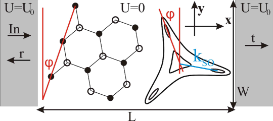
Figure 1: Geometry of a graphene device of length $L$ and width $W$ between two electrodes doped by potential $U_{0}$. Electrons incoming from the left lead are reflected with amplitudes $r$ and transmitted with amplitudes $t$. Between the two contacts we depict the real space structure of the monolayer graphene flake (left side) and the energy contours in reciprocal space around the $\mathbf{K}$ point. The zig-zag direction of the graphene flake makes an angle $\varphi$ with the electrode interface ($y$ direction).

2 Landauer–Büttiker formalism for calculating the conductivity

In the Landauer-Büttiker approach the conductance of a sample is given by the transmission probabilities of an electron passing through it:

$$G=\frac{e^{2}}{h}\sum\limits_{m,n}|t_{mn}|^{2},$$ (1)

where $t_{mn}$ are the transmission amplitudes between the propagating modes $n$ and $m$ of the left and right electrodes. In what follows, we calculate the minimal conductivity in the TB model (for finite $W$) and compare the results to that obtained in the continuous model (for $W\to\infty$). Both in TB and continuous model the transmission amplitudes $t_{mn}$ are calculated by solving the scattering problem of the system. Then the minimal conductivity is defined as $\sigma=\frac{L}{W}\,G$, with the conductance $G$ calculated from Eq. (1) at the charge neutral point of graphene, ie, at $E_{F}=0$.

2.1 Tight binding model of graphene including RSO coupling

In the TB model the Hamiltonian $H_{TB}$ of monolayer graphene with RSO coupling can be written as [22, 21]

$$H_{TB} =H_{0}+H_{R},\hskip 19.91692pt\text{where}$$ (2a)

$$H_{0} =-\gamma\sum\limits_{\left\langle i,j\right\rangle,\sigma}\left(a_{i\sigma}^{\dagger}b_{j\sigma}+{\rm h.c.}\right),$$ (2b)

$$H_{R} =i\,\lambda\sum\limits_{\left\langle i,j\right\rangle,\mu,\nu}\left[a_{i\mu}^{\dagger}\left(\boldsymbol{s}_{\mu\nu}\times\mathbf{\widehat{d}}_{\left\langle i,j\right\rangle}\right)_{z}b_{j\nu}-h.c.\right].$$ (2c)

Here $H_{0}$ is the Hamiltonian of bulk graphene sheet taking into account only nearest neighbor hopping, with hopping amplitude $\gamma$. The operator $a_{i\sigma}^{\dagger}$ ($a_{i\sigma}$) creates (annihilates) an electron in the $i$th unit cell with spin $\sigma$ on sublattice $A$, while $b_{j\sigma}^{\dagger}$ ($b_{j\sigma}$) has the same effect on sublattice $B$ and h.c. stands for hermitian conjugate. The unit cell is given by the unit vectors $\mathbf{a}_{1}$ and $\mathbf{a}_{2}$ as shown in Fig. 2. The Hamiltonian $H_{R}$ describes the Rashba spin-orbit interaction where $\boldsymbol{s}=(s_{x},s_{y},s_{z})$ are the Pauli matrices representing the electron spin, and $\mu,\nu=1,2$ denote the $\mu\nu$ matrix elements of the Pauli matrices. Here vectors $\mathbf{d}_{\left\langle i,j\right\rangle}$ connect the nearest neighbor atoms $\left\langle i,j\right\rangle$ pointing from $j$ to $i$ as shown in Fig. 2, and $d$ is the distance between them, and $\mathbf{\widehat{d}}_{\left\langle i,j\right\rangle}=\mathbf{d}_{\left\langle i,j\right\rangle}/d$ are unit vectors.

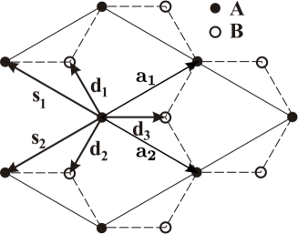
Figure 2: Geometry of a graphene sheet. The unit vectors of the hexagonal lattice are $\textbf{a}_{1}$ and $\textbf{a}_{2}$, while $\textbf{d}_{1}=(\textbf{a}_{2}-2\textbf{a}_{1})/3$, $\textbf{d}_{2}=(\textbf{a}_{1}-2\textbf{a}_{2})/3$ and $\textbf{d}_{3}=(\textbf{a}_{1}+\textbf{a}_{2})/3$ are vectors pointing to the neighboring atoms.

The strength of the spin-orbit coupling is denoted by $\lambda$ which may arise due to a perpendicular electric field or interaction with a substrate.

Using the standard Green’s function techniques [23, 24, 25] based on the Landauer–Büttiker approach we calculate the transmission amplitudes for armchair and zig-zag orientation of the sample.

2.2 Continuous model of graphene including RSO coupling

The Hamiltonian of the continuous model as a long wave approximation of the TB Hamiltonian $H_{TB}$ in Eq. (2) describes low energy excitations around the $\mathbf{K}$ and $\mathbf{K}^{\prime}$ points. In our previous publication [21] we showed that starting from the tight-binding Hamiltonian suggested in Ref. [22] to describe RSO coupling in monolayer graphene one can arrive at a form of the Hamiltonian that is unitary equivalent to that of bilayer graphene without RSO interaction but including the trigonal warping effect due to interlayer hopping [10, 15]. In the continuous model the Hamiltonian $H_{K}$ at the $\mathbf{K}$ point of the Brillouin zone (BZ) reads as:

$$H_{K}=\begin{pmatrix}0&v_{F}p_{-}&0&v_{\lambda}p_{+}\\ v_{F}p_{+}&0&-3i\lambda&0\\ 0&3i\lambda&0&v_{F}p_{-}\\ v_{\lambda}p_{-}&0&v_{F}p_{+}&0\end{pmatrix}$$ (3)

where $v_{F}=3\gamma d/(2\hbar)$, $v_{\lambda}=3\lambda d/(2\hbar)$, $p_{\pm}=p_{x}\pm ip_{y}$ and $p_{x},p_{y}$ are momentum operators. The Hamiltonian $H_{K}$ in Eq. (3) is written in the basis ${(|A\uparrow\rangle,|B\uparrow\rangle,|A\downarrow\rangle,|B\downarrow\rangle)}^{T}$ where $\{\uparrow,\downarrow\}$ refer to spin orientations. A unitary equivalent result can be obtained around the Dirac point $\mathbf{K}^{\prime}$. The four eigenvalues of the Hamiltonian (3) as a function of the wave number $\mathbf{k}=(k_{x},k_{y})=k(\cos\alpha,\sin\alpha)^{T}$ are given by

$$E_{n}^{\pm}(\mathbf{k}) =\pm\hbar v_{F}\,\sqrt{\frac{1}{2}\left[k_{\lambda}^{2}+k^{2}\left(2+\beta^{2}\right)+(-1)^{n}\sqrt{\Upsilon}\right]},\,\,\,\textrm{with}$$ (4a)

$$\Upsilon =k_{\lambda}^{4}+2k^{2}k_{\lambda}^{2}(2-\beta^{2})+k^{4}\beta^{2}(4+\beta^{2})-8k^{3}k_{\lambda}\beta\sin(3\alpha),$$ (4b)

where $$\beta=v_{\lambda}/v_{F}=\lambda/\gamma k_{\lambda}=2\beta/d n=1,2$$ is the dimensionless strength of the spin-orbit coupling, and .

Figure 3 shows the contour plot of the positive and low-energy band $E_{1}^{+}$ and the spectrum along the $k_{y}$ direction.

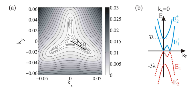
Figure 3: (a) Contour plot of the positive and low-energy band $E_{1}^{+}$ (in units of $\lambda$) around the $\mathbf{K}$ point for $\beta=0.034$. Wave vector components $k_{x}$, $k_{y}$ are in units of $3\lambda/(\hbar v_{F})$. The center of the pockets has a $2\pi/3$ rotational symmetry. The distance between the center of the pockets and the central Dirac points (points $\mathbf{K}$) is $k_{\textrm{SO}}$ given in the text. (b) The four energy bands along the direction $k_{y}$ with $k_{x}=0$.

The spectrum has a threefold symmetry similar to that of bilayer graphene. At moderate energy, direct hopping between $\Psi_{A\uparrow}$ and $\Psi_{B\downarrow}$ leads to trigonal warping of the constant energy lines about each valley, but at an energy $E$ less than the Lifshitz energy $E_{L}=\gamma\beta^{2}/(4+\beta^{2})$ the effect of trigonal warping is dramatic. It leads to a Lifshitz transition [26]: the constant energy line is broken into four pockets, which we refer to as central and three leg parts. The Fermi surface is approximately triangle like in the central part and each leg part it is elliptical. The distances of the center of the leg parts from the $\mathbf{K}$ point are $k_{\textrm{SO}}=2\beta^{2}/d$ (see Fig. 3).

As it has been shown in our previous work [15] the Lifshitz transition strongly affects the transport properties of monolayer graphene as well. The anisotropy of the minimal conductivity in bilayer graphene related to the interference effects between the leg parts was predicted by Moghaddam et al. [16]. Therefore, in monolayer graphene including the RSO interaction, we also expect a strong anisotropy in its conductivity depending on the orientation of the leg parts with respect to the electrodes. To see this we calculate the transmission probabilities $t_{mn}$ in Eq. (1) and the minimal conductivity by solving the scattering problem. If we consider the short and wide junction limit ($W\gg L$), then the electronic states can be specified by their energy $\varepsilon$ and the transverse wavenumber $q$ which are conserved during the scattering process. For a given $\varepsilon$ and $q$ there are four solutions for the longitudinal wave vector $k^{l}$ which satisfies the characteristic equation $\det\left[H_{K}(k^{(l)},q)-I_{4}\,\varepsilon\right]=0$, where $I_{4}$ is the $4\times 4$ identity matrix. Electronic states in the scattering region ($0\leq x\leq L$) are denoted by $\Psi_{\text{sc}}^{l}(q)=\Phi_{\text{sc}}^{l}e^{i(k^{l}x+qy)}$, where $\Phi_{\text{sc}}^{l}$ satisfy relation for all possible quantum numbers $l$:

$$H_{K}(k^{l},q)\,\Phi_{\text{sc}}^{l}=\varepsilon\,\Phi_{\text{sc}}^{l}.$$ (5)

The scattering state between the electrodes is then a linear combination of these four electronic states. The longitudinal wave numbers $k_{L/R}^{n}$ and the corresponding electronic states $\Psi_{L/R}^{n}(q)=\Phi_{L/R}^{n}\,e^{i(k_{L/R}^{n}x+qy)}$ in the left (L) and right (R) leads can be obtained analogously with a substitution $\varepsilon\rightarrow\varepsilon-U_{0}$ (here $U_{0}$ is the potential on the left and right electrodes as indicated in Fig. 1. If we assume an incident states in the L electrode, than the resulted scattering state can be written in the form:

$$\Psi^{n}(q)=\left\{\begin{array}[]{ll}\Psi_{L}^{n,\rightarrow}(q)+\sum\limits_{n^{\prime}=1}^{2}r_{n^{\prime}n}(q)\Psi_{L}^{n^{\prime},\leftarrow}(q),&x<0,\\ \sum\limits_{l=1}^{4}A_{p}\Psi_{\text{sc}}^{(l)}(q),&0\leq x\leq L,\\ \sum\limits_{m=1}^{2}t_{mn}(q)\Psi_{R}^{m,\rightarrow}(q),&L<x,\end{array}\right.$$ (6)

where $r_{n^{\prime}n}(q)$ and $t_{mn}(q)$ are the reflection and transmission amplitudes, and we introduced the arrow $\rightarrow$ ($\leftarrow$) to label the right (left) propagating electron states in the leads. The reflection and transmission amplitudes have to be determined (together with coefficients $A_{n}$) by imposing the continuity condition of the wave functions at the interfaces $x=0$ and $x=L$.

Finally, inserting the transmission probabilities $t_{mn}(q)$ into Eq. (1) we find the conductance $G$. The summation over the transverse wave numbers is replaced in a good approximation by the integration $\frac{W}{2\pi}\int\textrm{d}q$. Then the minimal conductivity reads:

$$\sigma=2\,\frac{L}{W}\,G=\frac{\sigma_{0}}{4}\,L\int\limits_{-\infty}^{\infty}{\rm d}q\sum\limits_{m,n}\left|t_{mn}(q)\right|^{2},$$ (7)

where in the first equation the factor 2 corresponds to the valley degeneracy.

3 Results: the minimal conductivity of monolayer graphene with RSO interaction

The minimal conductivity as function of $L$ obtained from the continuous model and from TB calculations for zig-zag and armchair orientation are shown in Fig. 4.

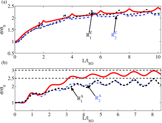
Figure 4: (Color online) The conductivity (in units of $\sigma_{0}$) of the junction as a function of length $L$ (in units of $l_{SO}$) for (a) zigzag and (b) armchair orientation in continuous model obtained from Eq. (7) (red solid lines) and from TB calculation (blue dash-dotted and black dashed lines) with two different aspect ratios $R_{1}^{Z}=W/L=4.71$ and $R_{2}^{Z}=W/L=6.74$ for zigzag orientation, and $R_{1}^{A}=W/L=3.12$ and $R_{2}^{A}=W/L=5.80$ for armchair orientation. The two horizontal dashed lines in Fig. b represent the upper limit of the conductivity calculated from the continuous ($3\sigma_{0}$) and TB model ($\frac{5}{2}\,\sigma_{0}$) as described in the text.

As described in Ref. [16] the RSO interaction can be characterized by a length scale $l_{SO}=\pi/k_{\textrm{SO}}\sim 1/\lambda^{2}$. For short junctions or at low RSO coupling $\lambda$, that is in the limit $L/l_{SO}\to 0$, the conductivity for both the armchair and zig-zag orientation starts with $\sigma(L/l_{SO}=0)=\sigma_{0}$. Increasing $L/l_{SO}$ the conductivity calculated from the continuous model tends to $\sigma=3\sigma_{0}$ and $\sigma=7/3\,\sigma_{0}$ for the armchair and zig-zag orientation, respectively.

In the TB calculation for zig-zag orientation, depicted in Fig. 4a, the conductivity closely follows that of the continuous model and tends towards $\sigma_{TB}=7/3\,\sigma_{0}$ for longer junctions. Increasing the $W/L$ ratio the subtle peaks of the TB and continuous models approach each other. On the other hand, for the armchair orientation, shown in Fig. 4b, the results of the TB calculation and the continuous model start to deviate for $L/l_{SO}\gtrapprox 1.1$, that is for increased RSO coupling $\lambda$, tending to a markedly lower value $\sigma_{TB}=5/2\,\sigma_{0}$. We also observe an enhanced oscillatory behavior as the function of $L/l_{SO}$ as compared to the calculation done in the zig-zag direction.

To understand this behavior of the conductivity it is instructive to consider the orientation of the Fermi surface around the $\mathbf{K}$ and $\mathbf{K}^{\prime}$points with respect to the direction of propagation as shown in Fig. 5. As noted before, trigonal warping due to the RSO interaction brakes the Fermi surface into a central pocket (dots in Figs. 5d and 5e at the $\mathbf{K}$ and $\mathbf{K}^{\prime}$points) and three extra leg pockets labeled by $P_{1}$, $P_{2}$ and $P_{3}$.

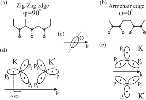
Figure 5: Schematic drawing of (a) zig-zag and (b) armchair edges. Empty circles and dashed lines correspond to the nearest missing sites and bonds to the edge of the ribbon. (c) The orientation of one pocket (an ellipse) is given by the angle $\Theta$ between the propagation direction ($k$ axis) and the semi-major axis of the ellipse. (d) Orientation of the pockets $P_{1}$, $P_{2}$, and $P_{3}$ for zig-zag and (e) for armchair edges in the Brillouin zone.

First we explain the oscillatory behavior of the conductivity shown in Fig. 4b for armchair orientation. In Fig. 5e the zero energy modes both around the $\mathbf{K}$ and $\mathbf{K}^{\prime}$ point are at the center of pocket $P_{1}$, $P_{2}$ and $P_{3}$, and at the center of the isotropic Dirac cone. Out of these four modes two (the central Dirac cone and pocket $P_{3}$) have a wave number $k=0$ (along the propagating direction) and for the other two modes the wave numbers are $k=\pm\frac{\sqrt{3}}{2}k_{\textrm{SO}}$ (the centers of pocket $P_{1}$ and $P_{2}$ in Fig. 5e. The latter two non-zero propagating modes explain the oscillatory behavior of the conductivity shown in Fig. 4b. The phase shift between the finite $k$ propagating modes (accumulated over one period) for an electron bouncing between the electrodes is $\Delta\Phi_{m}=\pm m\sqrt{3}k_{\textrm{SO}}L$, where $m=0,1,2$. Then the shortest period of the conductivity is given by $\Delta\Phi_{1}=2\pi$ from which one finds

$$\frac{L}{l_{SO}}=\frac{2}{\sqrt{3}}\approx 1.15.$$ (8)

This periodicity can be clearly seen in Fig. 4b for both TB and continuous cases.

In the case of the zig-zag orientation all pockets are centered at finite $k$. In both valleys the centers of the central pocket and pocket $P_{3}$ are separated by $k_{SO}$. this gives $L/l_{SO}=2$ as the shortest modulation period in agreement with our data presented in Fig. 4a.

Now we explain the marked discrepancy between the continuous model and the TB calculations performed in the armchair orientation. For strong RSO interaction the conductivity calculated in the tight binding approach can be estimated as follows. In general each pocket $P_{1},P_{2}$ and $P_{3}$ shown in Fig. 5 corresponds to one anisotropic Dirac cone and gives a separate contribution to the conductivity. The total conductivity is given by

$$\sigma =n_{C}\sigma_{C}+\sum_{i}n_{i}\sigma(\Theta_{i}),\,\,\,\text{where}$$ (9a)

$$\sigma(\Theta_{i}) =\frac{v_{a}^{2}\cos^{2}(\Theta_{i})+v_{b}^{2}\sin^{2}(\Theta_{i})}{v_{a}v_{b}}\frac{\sigma_{0}}{4},$$ (9b)

and $\sigma_{C}=\sigma_{0}/4$ is the contribution from the central Dirac cone [11] while $\sigma(\Theta_{i})$ is the minimal conductivity related to a single anisotropic Dirac cone. This result was first derived by Nilsson et al. in Ref. [27]. Note that the same result can be obtained by the general approach developed in Ref. [13]. Here $n_{C}$ and $n_{i}$ are the number of open channels for the central Dirac cone and the leg pocket $P_{i}$, respectively, and $v_{a}$ and $v_{b}$ are the Fermi velocities along the two principal axes of the ellipse corresponding to the pocket $P_{i}$ with $i=1,2,3$. For our case $v_{b}=3v_{a}$ [27] for the three legs. $\Theta_{i}$ is the angle of the direction of the semi-major axis of the ellipse with respect to the direction of propagation (see Fig. 5c). One can see from Fig. 5 that around the $\mathbf{K}$ point for armchair orientation $\Theta_{i}=7\pi/6;11\pi/6;\pi/2$ for pocket $P_{1}$, $P_{2}$ and $P_{3}$, respectively, while for zig-zag orientation $\Theta_{i}=5\pi/3;\pi/3;\pi$ around the $\mathbf{K}$ point, and $\Theta_{i}=4\pi/3;2\pi/3;0$ around the $\mathbf{K}^{\prime}$ point for the pocket $P_{1}$, $P_{2}$ and $P_{3}$, respectively (see Fig. 5).

We now determine the number of open channels $n_{C}$ and $n_{i}$ in Eq. (9). The boundary condition for the system demands that the wave function at the two edges of the ribbons should be zero at the empty sites shown schematically in Figs. 5a and 5b. Thus, including the spin we have four equations to satisfy the boundary conditions. For a given energy $\varepsilon$ and wave number $k$ corresponding to the propagating mode the possible transverse modes can be calculated from the dispersion relation. Graphically it means that these transverse modes can be obtained by drawing a vertical line at a given $k$ that intersects the given constant energy $\varepsilon$ contour. For example, for zig-zag orientation for wave number $k$ for which the vertical line passes through the center of pocket $P_{3}$ around the $\mathbf{K}$ point there are two transverse modes (the vertical line crosses the energy contour at two points in Fig. 5d, while for wave number $k$ for which the vertical line passes through the center of pockets $P_{1}$ and $P_{2}$ we have four transverse modes. Hence, it follows that in the first case the number of open channels $n_{1}=0$ since the four boundary conditions cannot be satisfied by two transverse modes. Similarly, for the central isotropic Dirac cone $n_{c}=0$. However, for the second case $n_{1}=n_{2}=1$ because we have four transverse modes. The same is true for the propagating mode $k$ around the $\mathbf{K}^{\prime}$ point (valley degeneracy). In summary, the open channels for zig-zag ribbons are $n_{C}=0$ and $n_{1}=n_{2}=2,n_{3}=0$. From a similar consideration we find that for armchair orientation $n_{C}=2$ and $n_{1}=n_{2}=1,n_{3}=2$. Thus the minimal conductivity of monolayer graphene with RSO coupling given by (9) is $\sigma=7/3\,\sigma_{0}$ for zig-zag and $\sigma=5/2\,\sigma_{0}$ for the armchair orientation, in very good agreement with the TB calculations.

4 Conclusions

We have investigated the minimal conductivity of monolayer graphene in the presence of Rashba spin-orbit interaction. We have employed tight binding calculations and a continuous model, to determine the interplay of the crystallographic orientation of the sample with the anisotropic nature of the minimal conductivity. Contrasting the results obtained for a graphene strip of finite width to that of an infinitely wide sample, we show that the boundary condition for a finite flake may, depending on the orientation, reduce the value of the minimal conductivity compared to that of the infinitely wide. All our calculations have been performed in the spirit of the Landauer-Büttiker approach. We hope our results are a tribute for the long lasting legacy of this simple yet powerful formalism and to the memory of Markus Büttiker.

References

References

- [1] R. Landauer, IBM J. Res. Dev. 1 (1957) 223.
- [2] M. Büttiker, Phys. Rev. Lett. 65 (1990) 2901–2904.
- [3] C. W. J. Beenakker, H. van Houten, Solid State Phys. 44 (1991) 1–228.
- [4] S. Datta, Electronic Transport in Mesoscopic Systems, Cambridge University Press, Cambridge, England, 1995.
- [5] T. Heinzel, Mesoscopic Electronics in Solid State Nanostructures, Wiley-VCH GmbH & Co. KGaA, Weinheim, 2003.
- [6] L. L. Sohn, L. P. Kouwenhoven, G. Schön (Eds.), Mesoscopic Electron Transport, Kluwer Academic Publishers, Dordrecht, The Netherlands, 1997.
- [7] K. Novoselov, A. Geim, S. Morozov, D. Jiang, Y. Zhang, S. Dubonos, I. Grigorieva, A. Firsov, Science 306 (2004) 666–669.
- [8] A. H. C. Neto, F. Guinea, N. M. R. Peres, K. S. Novoselov, A. K. Geim, Rev. Mod. Phys. 81 (2009) 109–162.
- [9] K. S. Novoselov, E. McCann, S. V. Morozov, V. I. Fal’ko, M. I. Katsnelson, U. Zeitler, D. Jiang, F. Schedin, A. K. Geim, Nature Physics 2 (2006) 177–180.
- [10] E. McCann, V. I. Fal’ko, Phys. Rev. Lett. 96 (2006) 086805.
- [11] J. Tworzydło, B. Trauzettel, M. Titov, A. Rycerz, C. W. J. Beenakker, Phys. Rev. Lett. 96 (2006) 246802.
- [12] M. I. Katsnelson, K. S. Novoselov, A. K. Geim, Nature Phys. 2 (2006) 620–625.
- [13] G. Dávid, P. Rakyta, L. Oroszlány, J. Cserti, Phys. Rev. B 85 (2012) 041402.
- [14] K. Ziegler, Phys. Rev. Lett. 97 (2006) 266802.
- [15] J. Cserti, A. Csordás, G. Dávid, Phys. Rev. Lett. 99 (2007) 066802.
- [16] A. G. Moghaddam, M. Zareyan, Phys. Rev. B 79 (2009) 073401.
- [17] A. Varykhalov, J. Sánchez-Barriga, A. M. Shikin, C. Biswas, E. Vescovo, A. Rybkin, D. Marchenko, O. Rader, Phys. Rev. Lett. 101 (2008) 157601.
- [18] private communication with Andrei Varykhalov.
- [19] K. Hasanirokh, H. Mohammadpour, A. Phirouznia, Physica E: Low-dimensional Systems and Nanostructures 56 (0) (2014) 227 – 230.
- [20] L. Razzaghi, M. V. Hosseini, Physica E: Low-dimensional Systems and Nanostructures 72 (2015) 89 – 94.
- [21] P. Rakyta, A. Kormányos, J. Cserti, Phys. Rev. B 82 (2010) 113405.
- [22] C. L. Kane, E. J. Mele, Phys. Rev. Lett. 95 (2005) 226801.
- [23] S. Sanvito, C. J. Lambert, J. H. Jefferson, A. M. Bratkovsky, Phys. Rev. B 59 (1999) 11936–11948.
- [24] I. Rungger, S. Sanvito, Phys. Rev. B 78 (2008) 035407.
- [25] P. Rakyta, E. Tóvári, M. Csontos, S. Csonka, A. Csordás, J. Cserti, Phys. Rev. B 90 (2014) 125428.
- [26] A. A. Abrikosov, Fundamentals of the Theory of Metals, Elsevier Science Publishers B. V., Amsterdam, North-Holland, 1988.
- [27] J. Nilsson, A. H. Castro Neto, F. Guinea, N. M. R. Peres, Phys. Rev. B 78 (2008) 045405.