A MUSE map of the central Orion Nebula (M 42) ^,

We present a new integral-field spectroscopic dataset of the central part of the Orion Nebula (M 42), observed with the MUSE instrument at the ESO VLT. We reduced the data with the public MUSE pipeline. The output products are two FITS cubes with a spatial size of $\sim 5\aas@@fstack{\prime}9\times 4\aas@@fstack{\prime}9$ (corresponding to $\sim 0.76\,\times\,0.63$ pc²) and a contiguous wavelength coverage of $4595\dots 9366$ Å, spatially sampled at $0\aas@@fstack{\prime\prime}2$. We provide two versions with a sampling of 1.25 Å and 0.85 Å in dispersion direction. Together with variance cubes these files have a size of 75 and 110 GiB on disk. They represent one of the largest integral field mosaics to date in terms of information content. We make them available for use in the community. To validate this dataset, we compare world coordinates, reconstructed magnitudes, velocities, and absolute and relative emission line fluxes to the literature and find excellent agreement. We derive a two-dimensional map of extinction and present de-reddened flux maps of several individual emission lines and of diagnostic line ratios. We estimate physical properties of the Orion Nebula, using the emission line ratios [N ii] and [S iii] (for the electron temperature $T_{\mathrm{e}}$) and [S ii] and [Cl iii] (for the electron density $N_{\mathrm{e}}$), and show two-dimensional images of the velocity measured from several bright emission lines.

1 Introduction

An H ii region is a diffuse nebula whose gas is heated and ionized by the ultraviolet radiation of early-type massive stars (see Shields, 1990; Osterbrock & Ferland, 2005). H ii regions are typically found in the arms of spiral galaxies and/or irregular galaxies and present spectra with strong emission lines visible even at cosmological distances. Galactic H ii regions in particular, can be seen as small-scale versions of the extreme events of star formation occurring in starburst galaxies (e. g. Weilbacher et al., 2003; Alonso-Herrero et al., 2009; García-Marín et al., 2009; Cairós et al., 2015). As such, they are laboratories offering an invaluable opportunity to study the interplay between recent and/or on-going star formation – in particular massive stars – and their surrounding interstellar medium, including gas and dust, at a high level of detail.

One of the best-studied Galactic H ii regions (and the closest) is the Orion Nebula (M 42), visible to the naked eye. It is often one of the first objects targeted with a new instrument; first, to see if something new can be discovered, and second, to use the plethora of existing observations for comparison, to validate a new system. A review about the nebula and its stellar content can be found in O’Dell (2001). Spectroscopic studies of the ionized gas, confined to one or several slit positions, have partially characterised the Orion’s emission spectrum (e. g. Baldwin et al., 1991; Pogge et al., 1992; Osterbrock et al., 1992; Mesa-Delgado et al., 2008; O’Dell & Harris, 2010).

However, H ii regions are rarely as simple as the textbook-like Strömgren (1939) spheres and Orion is no exception. Indeed, M 42 is thought to be only a thin blister of ionized gas at the near side of a giant molecular cloud (Zuckerman, 1973; Israel, 1978; van der Werf et al., 2013). To make most of the opportunity to observe an H ii region at the level of detail offered by Orion, spatially resolved maps with high-quality spectral information in terms of depth, spatial and spectral resolution are desirable.

Probably, the most efficient way to gather this information nowadays is the use of Integral Field Spectroscopy. Sánchez et al. (2007) released a first dataset based on this technique to the community (using the PPak-IFU of PMAS, Kelz et al., 2006), mapping most of the Huygens region – the central part of the nebula with the highest surface brightness. However, the data were taken under non-ideal weather conditions and hence, were poorly flux-calibrated. They were shallow due to very short exposure time and of low spatial and spectral resolution. Some of these aspects (depth and spectral resolution) were improved in a new mosaic mapping a similar area (Núñez-Díaz et al., 2013). However, the spatial resolution of these data were still relatively low. Also, at the moment, this improved dataset is not publicly available in reduced form. Additionally, there are several studies with very good data quality in terms of depth, spectral and spatial resolution, that were devoted to the study of invidiual targets within the Orion Nebula, and observed the interplay of gas and stars in proplyds and Herbig-Haro objects (e. g. Vasconcelos et al., 2005; Mesa-Delgado et al., 2011; Tsamis & Walsh, 2011; Mesa-Delgado et al., 2012; Tsamis et al., 2013; Núñez-Díaz et al., 2012). Therefore, they only mapped very small ($\sim$10″) rectangular areas. None of these currently existing datasets satisfy all of the following requirements: i) large mapped area, ii) depth, iii) ample spectral coverage, and iv) good spatial and spectral resolution.

Here, we present what we call true imaging spectroscopy of the Huygens region of the Orion Nebula, observed with the MUSE integral-field spectrograph mounted to VLT UT4 “Yepun”. MUSE comes close to producing the “perfect dataset” mentioned by O’Dell (2001): it samples the Huygens region with high spatial sampling (0$\aas@@fstack{\prime\prime}$2) and reasonable spectral resolution ($R\sim 3000$), and covers a large dynamic range.

Our aim in this work is twofold. On the one hand, from the technical point of view, this is one of the first sets of MUSE data and as such, it was taken with the main goal of testing offsets larger than the field of view and stress-test the data flow system related to the new instrument. On the other hand, from a scientific point of view, given the lack of a high-quality and science-ready set of spectrophotometric data of the whole Huygens region, we wanted to provide to the community with such data.

In this paper, we first describe the observations and the data reduction (Sect. 2), validate the new data against literature values (Sect. 3), describe a few unusual artifacts in the MUSE dataset (Sect. 4), and demonstrate how the MUSE datacube can be used for an analysis of both atomic and ionized gas (Sect. 5), before we conclude with a few general remarks (Sect. 6).

We assume a distance of $D=440$ pc (O’Dell & Henney, 2008) for the Orion nebula. This implies a linear scale of 0.0021 pc arcsec^-1. The field of view of the MUSE dataset then corresponds to $\sim 0.76\times 0.63$ pc².

2 Observations and Data Reduction

M 42 was observed as part of the first commissioning run (Bacon et al., 2014) of the MUSE instrument at the VLT. After some test exposures during the previous night, a uniform exposure time of 5 s per exposure was chosen as a compromise to not saturate the bright emission lines but give sufficient S/N in the outer regions. On 2014-02-16 between 01:02:59 and 03:34:31 (UTC), 60 exposures over a 6-by-5 mosaic were taken. Two exposures per position were observed, with the same center but alternating position angles of 0 and 90 degrees. The positions of the exposures are schematically shown in Fig. 1. To be able to create a contiguous grid, the positions were offset by 58″, which is somewhat smaller than the MUSE FOV.

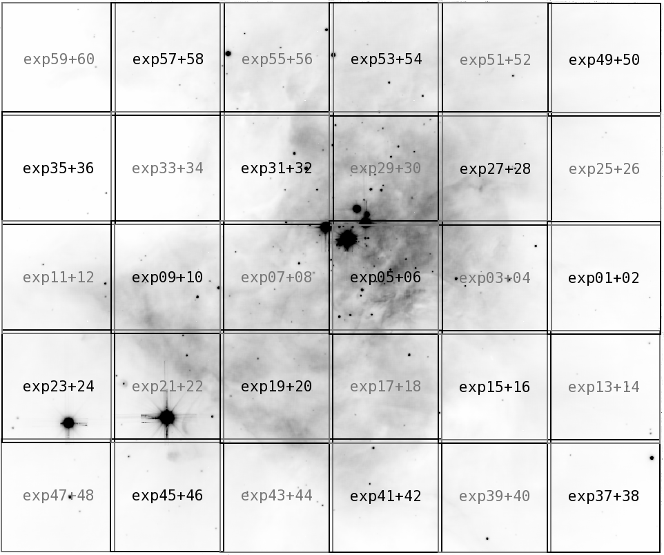
Figure 1: Inverse greyscale representation of the white-light image of the final mosaic. The positions of the observations are marked and annotated with the exposure numbers in the sequence from 1 to 60. Each box represents the approximate field of view of a single MUSE exposure, about $1\arcmin\times 1\arcmin$. The full field covered is $\sim 5\aas@@fstack{\prime}9\times 4\aas@@fstack{\prime}9$, centered on $\alpha=5^{\mathrm{h}}35^{\mathrm{m}}17\aas@@fstack{s}0$, $\delta=-5^{\circ}23\arcmin 43\arcsec$, with north to the top and east to the left.

Observation of the standard star GD 71 at 00:15:14 UTC and an airmass of 1.33 allowed a spectrophotometric calibration of the data. No sky exposures were taken. Daytime calibrations of the morning after the observing night were used.

The observing conditions were good, with photometric sky and DIMM seeing varying between 0$\aas@@fstack{\prime\prime}$67 and 1$\aas@@fstack{\prime\prime}$25. The M 42 mosaic was observed after transit, with airmass values ranging from 1.067 to 1.483. During the observations, the moon had an illumination of 95%, a distance of $\sim 87^{\circ}$ from the target, and rose from 10^∘ to 45^∘ in elevation.

The reduction used the dedicated MUSE pipeline (Weilbacher et al., 2012, Weilbacher et al. in prep.) through the EsoRex program. We used a development version of the pipeline, but the code was very close to the 1.0 release (patches are available on request).

For the basic calibration we followed the standard procedure to reduce MUSE data: combine 10 bias images to form a master bias, combine 5 lamp-flat exposures, and use one exposure of each arc lamp to derive the wavelength solution. 11 skyflats, taken during the evening twilight preceding the science exposures, were combined and used to create a 3D correction of the illumination in the range $\lambda=5000\dots 8000$ Å.

The geometry of the instrument was derived from a calibration sequence taken on 2014-02-05, the astrometric solution of the MUSE field of view was computed from an observation of a field in NGC 3201 on 2014-02-09. These calibrations were found to be valid for the full period of the first commissioning run of the instrument and were also shipped with the MUSE pipeline.

We then applied all calibrations to both the standard star exposure and all 60 science exposures, making use of a table of additional bad pixels of the CCDs that was created after the completion of MUSE commissioning runs, and which is shipped with the pipeline. For datasets with longer exposure time and lower contrast, the pipeline usually manages to correct the zero-order of the dispersion solution on a per-IFU basis using Gaussian fits as centroiding of bright sky emission lines. In the case of the M 42 mosaic, extreme contrast differences in some exposures and IFUs and the low sky emission background made this process unreliable. We therefore used the following procedure: we assume that the line [O i] 5577 is dominated by telluric emission (see e. g. Baldwin et al., 2000), so it was taken as baseline reference for each exposure and IFU. Since the shifts on the CCD are likely smoothly changing during the time of our observation, we iteratively fitted a linear relation to the MJD-OBS against the pipeline-computed wavelength offset, separately for each IFU. Deviant shifts were aggressively purged at the $2\sigma$ level. The wavelength zeropoint was then reset according to this linear relation with time.

Since the observations were done in extended mode, which incurs a 2nd order overlap at the red end of the wavelength coverage, the creation of the flux response curve needed extra care. We ran the pipeline recipe (muse_standard) with both circular flux integration and flux integration using Moffat profile fits. Circular apertures were used for wavelengths below 8334 Å, as they integrate slightly more flux than the Moffat fits and create a smoother response curve. Beyond 8430 Å, the circular aperture also integrates significant flux from the diffuse 2nd order, and the Moffat fit is a better representation of the total flux in the 1st order. At the transition wavelength, both curves have approximately the same slope and the curve from the Moffat fit was shifted slightly to account for the offset of both curves at this wavelength. The resulting merged response curve was again applied to the data of the standard star. A comparison of the reference spectrum with a spectrum extracted from that calibrated cube showed deviations typically below 5%.

The merged response and the astrometric calibration were then applied to each exposure individually. Creating and applying the response function used the average atmospheric extinction curve by Patat et al. (2011) as shipped with the MUSE pipeline. We let the pipeline automatically correct the atmospheric refraction (with the default method using the formula of Filippenko, 1982) and the barycentric velocity offset, but did not attempt to remove the sky background or the telluric absorption in the data. No attempts were made to homogenize the seeing along the wavelength direction, or between the 60 exposures.

All exposures were combined into a single cube. Since the observation strategy included rotation, the data were affected by the derotator wobble, so that each exposure had to be repositioned slightly. Luckily, each pointing contained at least one star that was also listed in the 2MASS catalog (Skrutskie et al., 2006), so we used the 2MASS positions as reference for the offsets that were applied when reconstructing the full cube. The effect is that the absolute astrometry of the final cube is tied to the 2MASS coordinates, similar to the HST mosaic of the Orion Nebula (Robberto et al., 2013).

We created a first full cube with the standard pipeline sampling of $0\aas@@fstack{\prime\prime}2\times 0\aas@@fstack{\prime\prime}2\times 1.25\,\AA$. However, as discussed below, we then chose a higher wavelength sampling for the final cube, to partially overcome the undersampling of MUSE data in the dispersion direction. Hence, a second cube was reconstructed with a sampling of $0\aas@@fstack{\prime\prime}2\times 0\aas@@fstack{\prime\prime}2$ spaxel^-1 in spatial and a linear step of $0.85$ Å pixel^-1 in wavelength direction. We call this cube the HR|0.85 cube while the cube with the standard sampling is the LR|1.25 cube. Both cubes have approximately the same wavelength coverage of $4595\dots 9366$ Å. The extent on the sky is exactly the same, $5\aas@@fstack{\prime}88\times 4\aas@@fstack{\prime}92$, but patches up to about 10 spaxels at the edge are not covered by data and filled with NaN values. The total size of the cubes is $1766\times 1476\times 3818$ voxels for LR|1.25 and $1766\times 1476\times 5614$ for HR|0.85 and they are stored in units of $10^{-20}\,\mathrm{erg}\,\mathrm{s}^{-1}\,\mathrm{cm}^{-2}\,$Å^-1 in the DATA extension of the FITS file. The MUSE pipeline also reconstructs a variance ($\sigma^{2}$) cube and stores it in the STAT extension in the same file. Several image extensions are available as well, averaging the cube either using known filter functions, or using constant weights across interesting wavelength ranges around some lines (see Table 1 for details). These image extensions are thought to be used only to locate interesting features in the cube, not for scientific analysis. The file size of the full dataset is 75 GiB (LR|1.25) and 110 GiB (HR|0.85).

For the purpose of the demonstration in this paper, we finally decided to use the LR|1.25 data for everything except the spatially resolved velocity analysis of the ionized gas, where HR|0.85 gives much lower systematic structures (see Sect. 3.4). However, the spatial calibration and the spectrophotometric accuracy is exactly the same for the HR|0.85 data, so the values quoted for the data quality in sections 3.1, 3.3, 3.5, and 3.6 refers to both datasets.

Table 1: FITS extensions in the provided files^a

EXTNAME	$\lambda$-range [Å]	comment
DATA	4595.00…9366.05	data values
STAT	4595.00…9366.05	data variance
white	4650.00…9300.00
Johnson_V		$V$-band filter
Cousins_R		$R$-band filter
Cousins_I		$I$-band filter
Halpha	6556.78…6568.78	H$\alpha$
NII_both	6542.06…6554.06,	both [N ii] lines…
	6577.39…6589.39	…(6548 and 6584)
Halpha_NII_OFF	6533.05…6538.05,	off-band for H$\alpha$ …
	6593.40…6598.40	…and [N ii]
OIII_both	4953.92…4965.92,	both [O iii] lines…
	5000.85…5012.85	…(4959 and 5007)
OIII_OFF	4969.92…4996.85	off-band for [O iii]
Hbeta	4855.32…4867.32	H$\beta$
Hbeta_OFF	4846.32…4851.31,	off-band…
	4871.33…4876.32	…for H$\beta$

^a the upper part of the table contains both data cubes, the middle part the images from standard pipeline filters, and the bottom images from specially created filters

3 Fidelity of the data

Since MUSE is a new instrument and the data reduction software is new, we have to carefully check the fidelity of the data to ensure its scientific usefulness.

3.1 Accuracy of the coordinate system

To verify the accuracy of the world coordinate system (WCS) in the MUSE cube, we determine positions in the reconstructed image integrated over the Johnson $V$ filter (extension Johnson_V in the FITS file). Applying daofind in IRAF to this image yields 259 detections, some of which are spurious sources.

Matching the list of point sources detected in MUSE to the 2MASS catalog (Skrutskie et al., 2006) results in 96 matches closer than 1″. After removing spurious sources, undetected double stars (listed as source in the 2MASS catalog), and stars saturated in the MUSE cube, we are left with 90 matched sources. Their separations are $0\aas@@fstack{\prime\prime}108\pm 0\aas@@fstack{\prime\prime}072$ (mean and standard deviation, or $0\aas@@fstack{\prime\prime}097\pm 0\aas@@fstack{\prime\prime}045$ using median and median absolute deviation). Using the same procedure, but matching MUSE detections against the HST ACS catalog of the Orion Nebula cluster as given by Robberto et al. (2013), we find 83 valid matches, giving an overall agreement of $0\aas@@fstack{\prime\prime}163\pm 0\aas@@fstack{\prime\prime}078$ (mean and standard deviation). This is in line with the accuracy of the HST catalog matched against 2MASS point sources (max. allowed separation 0$\aas@@fstack{\prime\prime}$5, resulting in $0\aas@@fstack{\prime\prime}138\pm 0\aas@@fstack{\prime\prime}085$) and comparable to the astrometric accuracy of the 2MASS point source catalog itself, $\lesssim 100$ mas given in Skrutskie et al. (2006).

3.2 Quality of the atmospheric refraction correction

Since the atmospheric refraction present in the raw MUSE data was corrected by the pipeline reduction, compact sources in the field do not show strong gradients across several spatial pixels. Nevertheless, the formula to compute the refractive index of air (taken from Filippenko, 1982) is imperfect, so some residuals are left in the data.

We test the residuals using the centers of four bright stars in the field. The centers of the stars were measured in each wavelength plane of the final cube by two methods: 1. by fitting a Moffat function and 2. by computing the marginal centroid as with imcentroid in IRAF. The results are shown in Fig. 2.

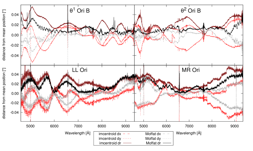
Figure 2: Centroiding residuals with wavelength for four bright stars in the field. Each panel shows horizontal and vertical distances to the mean center of the star in lighter dashed and dotted curves, and the radius as solid dark curve. Red curves are for imcentroid measurements, black lines for Moffat fits.

The strongest deviations from the mean centroid position of each star occur in regions of high background (strong nebular emission lines) and low throughput (telluric absorption). Ignoring these wavelength ranges, the typical deviations from the mean centroid position are smaller than 0$\aas@@fstack{\prime\prime}$05 or 1/4th of a spatial element of the cube.

3.3 Magnitudes and colors

We used the same stellar spectra already extracted using the Moffat fit in Sect. 3.2 to determine how well we can reproduce stellar magnitudes using the MUSE data.

Figure 3: Extracted spectra of four bright stars in the field; the flux is displayed in arbitrary logarithmic units, the individual spectra are scaled and offset for better visibility, and not in order of stellar magnitude.

The extracted spectra are shown in Fig. 3. The telluric absorption that is visible does not significantly affect measurement of the integrated magnitudes ($R$-band: 0.007 mag, $I$-band: 0.023 mag). Nevertheless, for this test, we replaced the absorbed regions in the spectrum with an average value before integrating the spectra over the filter functions (we used Johnson $V$, and Cousins $R$ and $I$).

The effect of nebular line emission that was not optimally subtracted by the Moffat fit is less certain. Indeed, LL Ori shows intrinsic Balmer and CaII-triplet emission that cannot be explained by residuals of nebular emission (see also Hillenbrand, 1997) whereas small residuals of [O iii] 5007 and [N ii] 6584 are very likely of nebular origin. Since the equivalent widths of the emission features are low – $\mathrm{EW}(\mathrm{H}\alpha)\approx-42.5$ Å for LL Ori – the influence on the broad-band magnitudes is rather low.

Table 2: Comparison of integrated magnitudes to the literature.

object	band	$m_{\mathrm{MUSE}}$ [mag]	$m_{\mathrm{lit}}-m_{\mathrm{MUSE}}$ [mag]
$θ^1$ Ori B	$V$	7.990	-0.031
	$R$	7.760
	$I$	7.422
$θ^2$ Ori B	$V$	6.389	0.0091, 0.0214
	$R$	6.403	-0.1041
	$I$	6.356	(4.6942,3), 0.0544
LL Ori	$V$	11.499	0.0182, 0.0214
	$R$	10.835
	$I$	10.218	-0.1842, -0.0384
MR Ori	$V$	10.551	0.0272
	$R$	10.286
	$I$	10.010	-0.1742

¹ compared to magnitude given by Ducati (2002)
² compared to magnitude given by Da Rio et al. (2009)
³ the value given by Da Rio et al. (2009) for $θ^2$ Ori B ($m_{I}=11.050$ mag) is clearly faulty
⁴ compared to magnitudes given by Hillenbrand (1997)

An agreement of a few hundreths of a magnitude in the $V$-band can be regarded as very satisfactory. The $V$-band differences quoted in Tab. 2 correspond to flux differences of up to 2.7%.

However, the comparison with $R$ and $I$ filters, where available, remains puzzling. Only the $I$-band magnitudes given in the table of Hillenbrand (1997) are close to our measurements, and these are only available for two of our four stars used for this experiment. As we have argued in Sect. 2 and checked in a different way in Sect. 3.6, differences of 0.1 to 0.18 mag or up to 18% in flux (as seen relative to the measurements of Ducati, 2002; Da Rio et al., 2009) are unlikely to be a problem with the relative flux calibration of the MUSE spectra, which is accurate to at least 5%.

To further investigate the difference, we also convolved our spectra with the filter plus CCD throughputs of the ESO WFI setup used by Da Rio et al. (2009). This made the agreement even worse. Since all stars in our field of view are likely variable at some level – of the four stars we analyzed here, all except $\theta^{2}$ Ori B are listed in the variable star catalog of (Samus et al., 2009) – one should not expect high precision of the comparison. But as variability likely affects observations in different filters in a similar way, this cannot explain the differences we see here. We therefore have to assume that the zeropoints applied by Da Rio et al. include an unknown component that causes a shift of the central effective wavelength of the red filters, but less of a shift for the green filter. Since the Orion Nebula is too bright for SDSS stellar photometry to work and all four stars are marked as saturated in the HST ACS catalog of Robberto et al. (2013), we cannot cross-check our reconstructed magnitudes with a better-studied photometric system.

3.4 Derived velocities

MUSE has a moderate velocity resolution (about 107 km s^-1 at 7000 Å), and the line spread function is slightly undersampled. As a consequence it is challenging to measure accurate velocity centroids for single narrow spectral features such as emission lines in HII regions. Nevertheless, we compare our derived velocities against the values given by Baldwin et al. (2000, hereafter B00).

The MUSE cube is corrected to barycentric velocities, so we can directly check our velocities against their heliocentric reference value of $+11.9$ km s^-1. If we extract a spectrum over the same aperture as the “blue” slit of B00, and fit all bright and a few fainter emission lines with Gaussian profiles, we can plot the resulting velocities for both of our cubes (LR|1.25 and HR|0.85) as well as the reference values from B00.

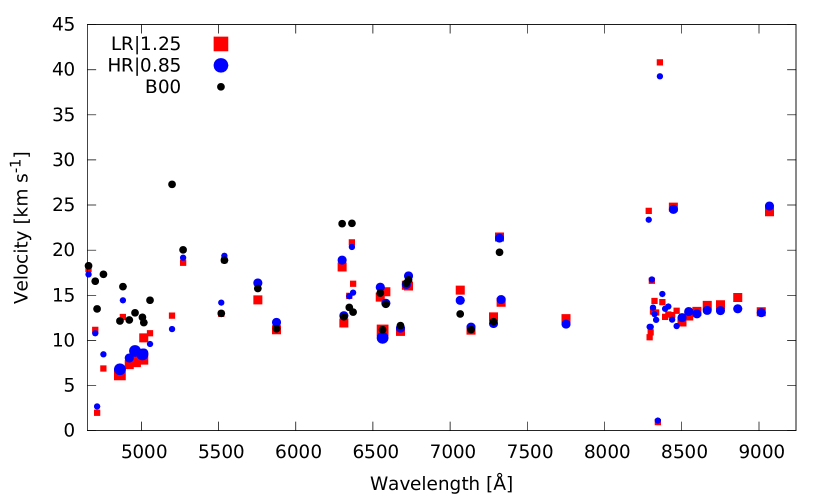
Figure 4: Velocities measured within the “blue” slit of Baldwin et al. (2000, B00). These are corrected to barycentric velocity for our data (red squares and blue circles) and to heliocentric for B00 (black circles). The point size of our measurements changes with the relative flux of the lines, such that the brightest lines have the largest symbols.

In Fig. 4 we show the result. We can reproduce the average velocity of about 12  km s^-1 reported by B00. This is seen for most of the Paschen lines in the very red (that were not measured in B00’s setup) and – with some scatter – for most other lines in the wavelength range $5250<\lambda<8000\,\AA$. The bright lines below 5250 Å, however, show a deviation from this mean velocity, in the sense that we measure velocities about 6  km s^-1 below those derived by B00. While the fainter lines at similar wavelengths do not all show this offset, they are partly blended with neighboring lines, and are therefore less trustworthy.

Several strong outliers are visible at the red end of the spectrum in Fig. 4. These are three of the fainter Paschen lines (Pa22, Pa23, and Pa30) and most likely due to blending with another unidentified weak line. However, the strong and relatively isolated lines OI 8446 and [S iii] 9069 also show a strong offset of $\sim 12$  km s^-1. Since the surrounding Paschen lines follow the normal trend very well, this casts doubts on the reliability of the reference wavelengths (we used 8446.462 and 9068.6 from the NIST database Kramida et al., 2014). Indeed, taking the reference value of 9068.9 Å as quoted by Osterbrock et al. (1992) for [S iii], we find a velocity of 14.35 and 14.97  km s^-1 for our LR|1.25 and HR|0.85 data, respectively, perfectly in line with the general trend.

We therefore conclude that in the range $\lambda<5250\,\AA$ the MUSE data likely shows a problem with the wavelength calibration, on the level of up to 0.1 Å (less than 1/10th of a MUSE pixel), while no systematic deviations larger than $\sim 3$  km s^-1 were found for wavelengths $\lambda>5250\,\AA$.

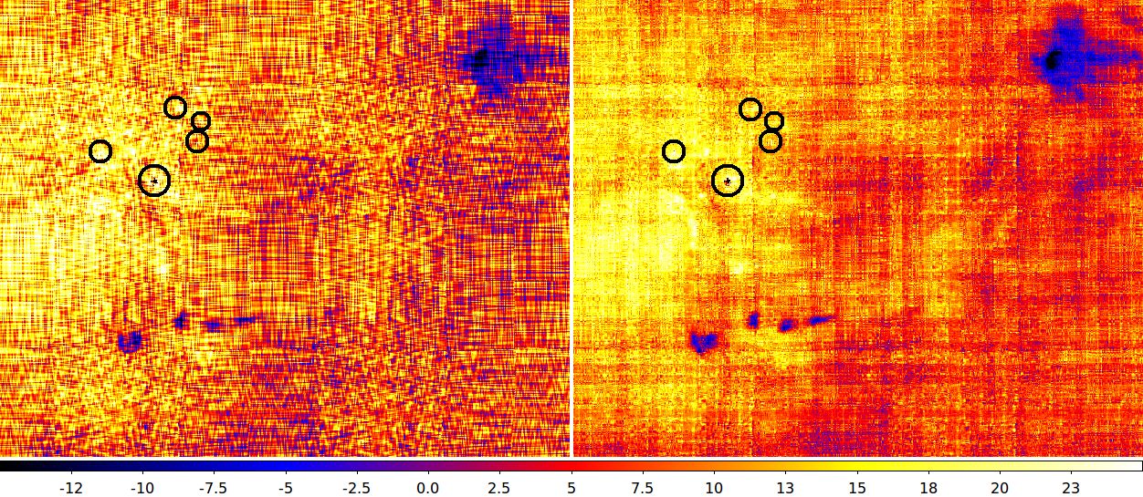
Figure 5: Velocity field as traced by the line [O iii] 5007, in part of the MUSE field of view. Left: using the LR|1.25 cube; right: using the HR|0.85 cube. The linear color scale is $v_{\mathrm{bary}}=-15\dots 25$ km s^-1, the brightest stars of the Trapezium cluster are marked as black circles.

We then compare maps of emission line velocities over the full field. These velocities were derived using single Gaussian profile fits to individual lines, and the maps show systematic patterns. These systematics are much more pronounced in the LR|1.25 cube than in the HR|0.85 data. This is demonstrated in Fig. 5, which shows the two-dimensional velocity field recovered from Gaussian centroids of the [O iii] 5007 emission line, for a part of the field around the Trapezium stars. The strong horizontal and vertical stripes show the influence of the per-slice sampling in the MUSE field of view on the derived velocity field. This effect is much reduced in the HR|0.85 cube, where the higher sampling of the line profile allows for more stable line fits. Only a residual pattern of the IFU structure is still visible (about 12 pixel wide stripes). For derivation of spatial velocity fields, it is therefore recommended to use the HR|0.85 cube.

To determine if the blue wavelength calibration problem discussed above is an absolute offset with wavelength or has gradients across the field, we also compute average and standard deviation of velocity difference maps for a few lines: we find $v(\mathrm{H}\alpha)=14.5\pm 5.9$ km s^-1 (LR|1.25) and $14.4\pm 4.5$ km s^-1 (HR|0.85), so that the overall velocity field in H$\alpha$ is very comparable between both datacubes. Taking the statistics from the difference map of H$\alpha$ and Pa$\zeta$, we find $v(\mathrm{H}\alpha)-v(\mathrm{Pa}\zeta)=-1.1\pm 9.6$ km s^-1 (LR|1.25) and $-1.0\pm 8.3$ km s^-1 (HR|0.85), i. e. a very good agreement between velocities derived from H$\alpha$ and the Paschen lines across the whole field of view. Comparing H$\alpha$ and H$\beta$ in the same way, we find a similar offset as discussed above for one slit position: $v(\mathrm{H}\alpha)-v(\mathrm{H}\beta)=4.9\pm 10.5$ km s^-1 (LR|1.25) and $4.9\pm 9.4$ km s^-1 (HR|0.85). We therefore conclude that the relative wavelength calibration across the field is very stable when measuring each emission line individually.

We also briefly compare the map shown in Fig. 5 with the literature. The velocities we measure are at odds with those measured by Rosado et al. (2001) using an optical Fabry-Pérot instrument, who find strongly blueshifted velocites (up to and around $-100$ km s^-1) over much of the nebula, in the H$\alpha$ line. In the vicinity of HH 203 they also find velocities of around $-75$ km s^-1 in the H$\alpha$ line, whereas we see $v\approx-20$ km s^-1 at the most blueshifted part of the same jet (also see Fig. 28). Our measurements are more comparable to the velocities measured in the near-infrared by Takami et al. (2002, with a different instrument also called MUSE), who see approximately $0$ km s^-1 in the region around the Trapezium stars, and $\sim-20$ km s^-1 in HH 203 in He i  10830 and approximately $-15$ km s^-1 in Pa$\beta$.

Since our data are of lower spectral resolution than some other studies, we should be sensitive only to high-velocity features in the primary component of each emission line. Since strong bipolarities as reported by e. g. Doi et al. (2004) around some proplyds are only detectable in fainter components – which in our data are blended with the main line profile – we cannot detect such features.

3.5 Absolute fluxes

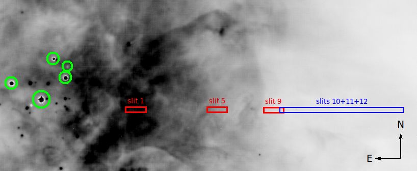
Figure 6: Literature slit positions taken from Baldwin et al. (1991) on top of a H$\beta$ flux map. The compass has an extent of 10″, the Trapezium stars are marked with green circles.

There are only few publications on the Orion Nebula which also quote absolute emission line fluxes; most rely on flux ratios. To check the flux calibration of our data, we extracted spectra at positions given in the literature. For this purpose, we used the regions functionality of DS9 which allowed easy, interactive placement of rectangular boxes onto the WCS positions, approximating the given slit lengths and widths. Then, the “3D plot” function was used to create spectra summed over these regions.

Following the example of O’Dell & Harris (2010, hereafter ODH10), we first extracted a 96$\aas@@fstack{\prime\prime}$8 box corresponding to the corrected position (4″ south of $\theta^{1}$ Ori C as described in ODH10) for slits 10+11+12 of Baldwin et al. (1991, hereafter B91). The positions of the slits reproduced on top of the MUSE data are displayed in Fig. 6. We then measured the principal emission lines for comparison using Gaussian fits with splot in IRAF We find $F_{\mathrm{H\beta}}=1.623\times 10^{-13}\,\mathrm{erg}\,\mathrm{s}^{-1}\,\mathrm{cm}^{-2}\,\mathrm{arcsec}^{-2}$, i.e. a 6% difference to B91 ($1.73\times 10^{-13}$ but 14.6% difference to the measurement of $1.90\times 10^{-13}$ by ODH10).

Table 3: Comparison of H$\beta$ flux measurements with the literature.

slit	$F_{\mathrm{H\beta,literature}}$	$F_{\mathrm{H\beta,MUSE}}$	rel. change
B91a slit 10+11+12	$1.73\times 10^{-13}$	$1.623\times 10^{-13}$	6.2%
c.f. ODH10b	$1.90\times 10^{-13}$	$1.623\times 10^{-13}$	14.6%
B91 slit 1	$9.99\times 10^{-13}$	$1.229\times 10^{-12}$	-23.0%
B91 slit 5	$7.39\times 10^{-13}$	$5.314\times 10^{-13}$	28.1%
B91 slit 9	$2.22\times 10^{-13}$	$2.210\times 10^{-13}$	0.5%
B91 slit 9, 2″ E c	$2.22\times 10^{-13}$	$2.532\times 10^{-13}$	-14.1%
B91 slit 9, 2″ W c	$2.22\times 10^{-13}$	$2.064\times 10^{-13}$	7.0%
B91 slit 9, 2″ N c	$2.22\times 10^{-13}$	$2.136\times 10^{-13}$	3.8%
B91 slit 9, 2″ S c	$2.22\times 10^{-13}$	$2.273\times 10^{-13}$	-2.4%

^a B91 = Baldwin et al. (1991)
^b observations by O’Dell & Harris (2010) at position of B91
^c value measured by B91 in their slit 5 as reference

We carried out the same comparison for slits 1, 5, and 9 of B91, similarly correcting the position in declination. The results can be found in Tab. 3. The differences in absolute flux measurement are up to 28%, unexpectedly high, if the positions would be recovered perfectly. However, the discussion in ODH10 shows that the positions and widths used during longslit spectroscopic observations are rather uncertain, errors up to a few arc seconds may occur. We therefore briefly investigate what the effect of small shifts applied to the best recovered position have on the absolute fluxes of the H$\beta$ line. Applying 2″ (the width of the B91 slit) offsets to the position of slit 9 (the one that best recovers the flux determined by B91) in all 4 directions shows that flux difference of up to $\sim$15% can easily occur.

We therefore conclude that the main cause of the differences in absolute H$\beta$ flux with respect to literature values are likely caused by uncertainties in the slit positions we can recover.

3.6 Flux ratios

Flux ratios, relative to H$\beta$ or He i 6678 are given in many publications on the Orion Nebula. However, it is not always straightforward to reproduce the slit placement accurately enough to derive a meaningful comparison. E. g. the observations carried out by Osterbrock et al. (1992) and Baldwin et al. (2000) were located in regions of strong emission-line gradients. Additional problems, like the unknown effect of atmospheric refraction on the literature line ratios make the comparison even more difficult.

Table 4: Comparison of emission line ratios to the literature.

$\lambda$	ID		$F/F_{\mathrm{H\beta}}$		rel.	change
[Å]		B91a	ODH10b	MUSEc	$\frac{\mathrm{B91}}{\mathrm{MUSE}}$	$\frac{\mathrm{ODH10}}{\mathrm{MUSE}}$
4861.48	H$\beta$	1.00	1.00	1.000	0.0%	0.0%
4959.09	[O iii]	0.92	0.93	0.934	-1.5%	-0.4%
5007.03	[O iii]	2.76	2.75	2.813	-1.9%	-2.3%
6563.08	H$\alpha$	3.34	3.20	3.358	-0.5%	-4.9%
6716.81	[S ii]	0.061	0.058	0.057	5.9%	1.0%
6731.23	[S ii]	0.076	0.068	0.071	6.5%	-4.5%
7065.56	He i	0.047	0.048	0.049	-4.8%	-2.6%

^a flux ratio from Baldwin et al. (1991) as quoted by ODH10
^b flux ratio from O’Dell & Harris (2010) (their Tab. 1)
^c flux measured in MUSE data in the same area using Gaussian line fits

Finally, we reproduced the approach and slit placement of O’Dell & Harris (2010, ODH10), which has the advantage of being located in an area with shallower gradients. This also lets us compare again the relevant lines with Baldwin et al. (1991, B91).

We used our extracted spectrum and the measurement procedure that we already discussed in Sect. 3.5. The result is presented in Tab. 4, as fluxes relative to the H$\beta$ line. The MUSE result lies approximately between the measurements of B91 and ODH10, with maximum deviations of up to 6.5% to one of the references, with a maximum deviation of 3.7% to the mean of both reference measurements. This is the deviation expected given the flux calibration accuracy quoted in Sect. 2.

Since the night was photometric, we make no attempts to check other regions of our cube, but assume that the relative fluxes are accurate to $\sim 5$% over the full field.

4 Artifacts visible in the data

Potential users of the data should be aware of a few artifacts present in the data. Some of them are due to the imperfect calibrations taken at the time of the first commissioning with the MUSE instrument, others are instrumental features that are hard to model and hence cannot be removed. These effects will be described in detail by Bacon et al. (in prep.).

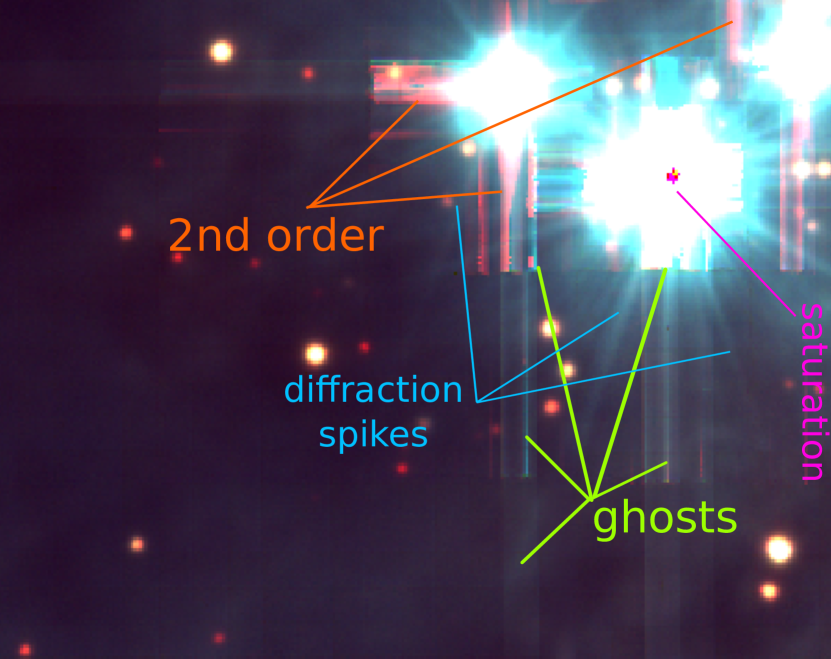
Figure 7: Color composite of the region near the Trapezium stars. The colors are created from continuum regions of the spectrum, with blue: 4600…4800 Å, green: 5300…5500 Å, and red: 9100…9200 Å. Ghosts are visible as blueish vertical and horizontal stripes, second order as reddish striping, and saturation as magenta pixels.

The brightest part of the data, the region around the Trapezium is particularly affected. Fig. 7 shows this region in a color composite, highlighting the continuum in three wavelength bands.

At all wavelengths, ghosts around bright objects are visible as vertical and horizontal stripes. These are likely due to internal reflections in the spectrographs, resulting in a faint background (at the level of $6\times 10^{-6}$, Bacon et al. in prep.) across the CCD, mostly affecting the slice in which the bright object is located but also neighboring slices. The cross-pattern this creates is due to the observations with the two position angles of 0 and 90 degree. Note that these ghosts are not the same as the usual diffraction spikes seen in pure imaging data. These exist in the MUSE data as well (see Fig. 7), but are fainter than the ghosts, and smoothly decrease with radial distance from the star.

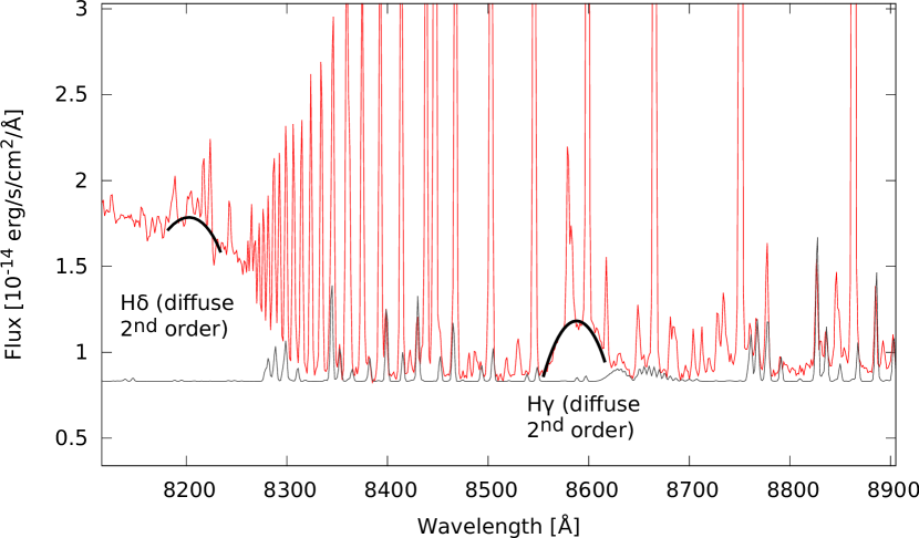
Figure 8: Spectral region around the Paschen limit. The red spectrum was extracted from the MUSE cube at the approximate position of slit1 of Baldwin et al. (1991). In grey, a typical Paranal sky spectrum is shown. Broad second order contamination by prominent blue Balmer emission lines is marked in black.

In the very red part of the spectrum, the second spectral order also becomes apparent. Since this order is unfocused in MUSE, it appears broadened compared to real features in the data. In Fig. 7 the 2nd order can be seen spatially, as red striping, again in horizontal and vertical directions. The second order is also visible in spectral direction, as displayed in Fig. 8. The nebular continuum is almost featureless, so this merely creates an additional offset, but strong emission lines in the blue can create broad bumps in the spectrum. However, if care is taken to locally fit or subtract the background when integrating line fluxes, these broad bumps should not cause any problems when extracting signal from the cube.

The brightest stars are also saturated near their peak. Part of this saturation appears as magenta pixels in Fig. 7. However, around the strongly saturated pixels, a few more pixels may be strongly negative, or have positive values below the real value. No attempts were made to mask these out.

Since neither telluric emission (Fig. 8) nor absorption (Fig. 14) were treated in our reduction, both still show up in extracted spectra. The nebular emission towards the Huygens region is very bright compared to the sky, most measurements are unaffected by more than a few percent. Notable exceptions are emission lines that are of comparable brightness to the sky background, such as [O i] 5577 or – in a few places where the nebula is faint – [O i] 6300.

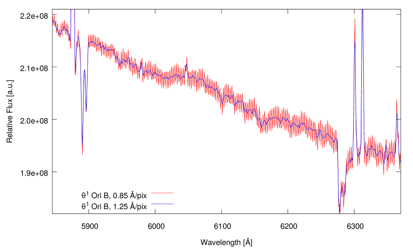
Figure 9: “Wiggles” in the extracted HR|0.85 spectrum of $\theta^{1}$ Ori B, compared with normal LR|1.25 spectrum.

When extracting spectra of (bright) point sources from the HR|0.85 MUSE cube, wiggles in the continuum can be seen (Fig. 9). The origin of this feature is not fully understood, but it is likely caused by a change of the spatial point-spread function (PSF), i. e. variations in seeing between exposures. Since the two exposures per position are interleaved in the final HR|0.85 cube and – depending on the exact sampling in the cube – often contribute to alternating wavelength planes, any variations in seeing between exposures effectively causes the PSF to also vary between adjacent planes in the cube. When integrating the flux of a star in an aperture that is too small to integrate the whole flux in both seeing conditions, the output spectrum looks particularly ‘wiggly’, as displayed in Fig. 9. The problem is mitigated when using PSF-matched spectral extraction (Kamann et al., 2013) where the PSF is fitted to each wavelength plane separately instead of using simple aperture extraction. We confirmed this by testing extraction strategies in a different MUSE two-exposure dataset (of a globular cluster, Kamann et al., in prep.) at LR|1.25 and HR|0.85 output sampling. However, since the PSF fit is imperfect, even then the wiggles do not completely disappear from HR|0.85 data. For stellar work, we therefore recommend use of the LR|1.25 cube where this problem does not occur at all. We were unable to detect this problem in the ionized gas. Since the spatial changes in the gaseous nebula are smoother, this problem only affects point sources but not the gas continuum or the emission lines.

5 Analysis of the ionized gas

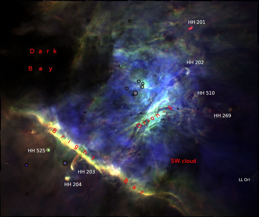
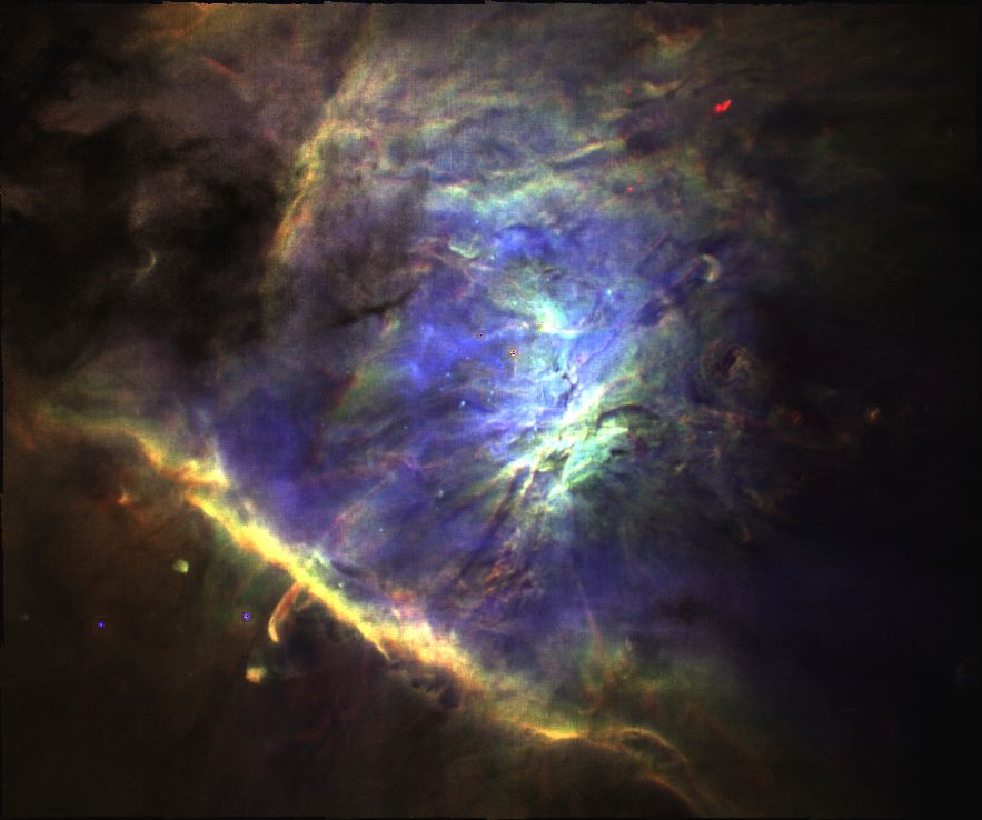
Figure 10: Color composite using fluxes of three emission lines, with blue: H$\beta$, green: [N ii] 6584, and red: [S ii] 6731. The brightest stars in the field are marked with black circles, large features are annotated in red text, other prominent features in white.

Figure 11: Color composite, created from the same emission lines as Fig. 13 but using the reddening-corrected fluxes, using the extinction estimate from the Balmer decrement.

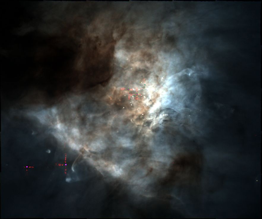
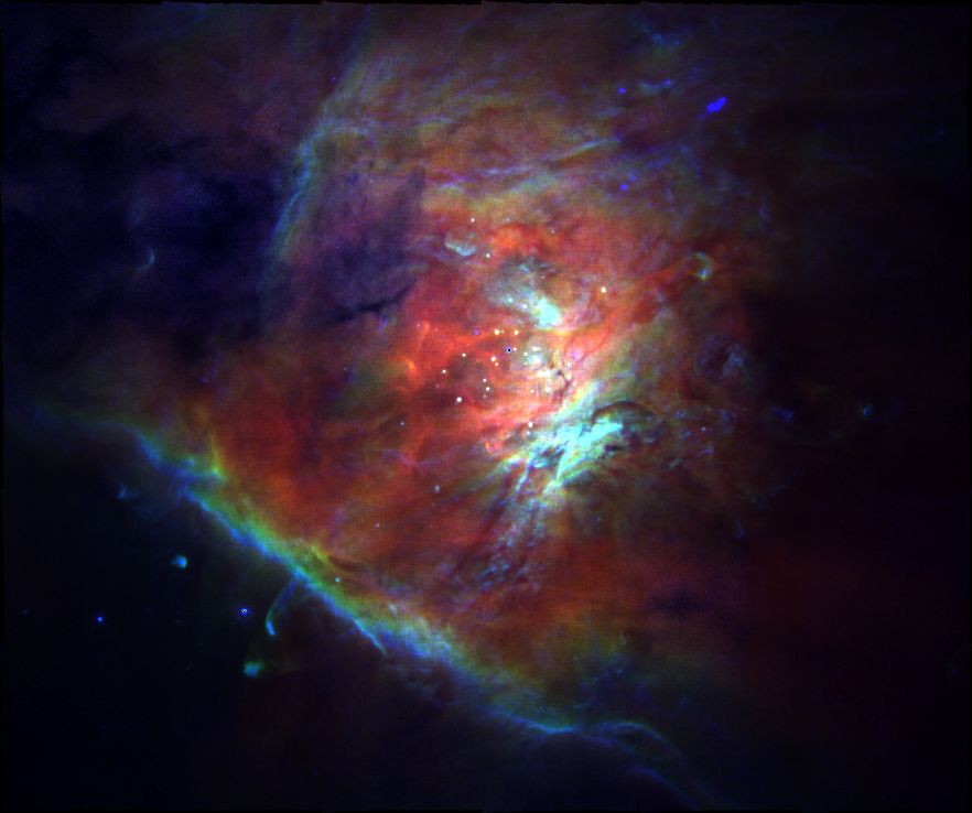
Figure 12: Color composite, using emission line fluxes of red: Paschen 9, green: H$\alpha$, blue: H$\beta$. In the red band, the effect of ghosts around bright stars is visible (cf. Fig. 7).

Figure 13: False color image, using the three ionization levels of oxygen detectable with the MUSE data: red: [O iii] 5007, green: [O ii] 7320, blue: [O i] 6300, all corrected for extinction using the Balmer decrement. [O i] is partially corrected for sky-line contribution. This representation shows the stratification of the nebula even more clearly than Fig. 13.

This section is devoted to show-case analysis methods that are possible with the MUSE data. All maps we show here were created using Gaussian fits to single emission lines. The fit was carried out on the LR|1.25 data, separately in each spaxel (using the HR|0.85 data gives almost identical results). We allowed variations in the flux of the line, its width, and the central position (restricted to be within 5 Å of the expected zero-redshift center). The fit also included a constant background offset. Since we did not attempt to mask stars before the fit, these show up as artifacts in some of the maps, especially for Balmer lines.

At the spectral resolution of MUSE, the line [O i] 6300 cannot be separated from the sky line at the same wavelength. We therefore assumed that the nebular line dominates the emission, but in the region of the Dark Bay (where the nebular line is weak) and especially in MUSE exposures 31 to 36, the sky line was stronger, leading to increased flux in the area covered by these exposures. We modeled this as a linear multiplicative gradient, decreasing from 1.34 at the left edge of the field to 1.0 at the approximate right edge of exposure 31+32 (cf. Fig. 1), and divided it out. Since we ignored other lines that coincide with telluric features, [O i] 6300 is the only line that was treated in this special way.

In Figures 13 to 13 we show different color representations, using the fluxes of three emission lines at a time, extracted from the MUSE data.

In Fig. 13, the selected lines trace different ionization states in the main ionization front and hence different distances from $\theta^{1}$ Ori C (O’Dell, 2001): [S ii] emission is produced in the layer of the main ionization front on top of the molecular cloud, [N ii] at intermediate distances, and H$\beta$ directly around the Trapezium cluster. The most striking features are the Bright Bar that runs across the image at the bottom left, and the Orion-S region – the brightest part of the nebula close to the main ionizing source – in the center. Since the stars are visible only as small and faint artifacts in this image, in the region to the SE of the Bright Bar, only a few Herbig-Haro objects are prominently visible: the jets of HH 203 and HH 204 (O’Dell & Wen, 1994) next to each other and the more roundish blob of HH 524 (Bally et al., 2000). In this image, we also note a spot with strongly enhanced [S ii] emission in the upper right that appears as a red clump in Fig. 13. This is HH 201, one of the “bullets” from the wide-angle Orion outflow (Graham et al., 2003; Bally et al., 2015). Compared to the surrounding material, it is similarly bright in [O i] 6300. In the MUSE data, we detect a secondary (blueshifted) component in the velocity field of these emission lines in this region.

Fig. 13 shows the same image but corrected for extinction using the Balmer decrement (see Sect. 5.1). Fig. 13 combines the emission line fluxes of three hydrogen lines spread over almost the full MUSE wavelength range: Paschen9 (= Pa$\zeta$) at 9229.7 Å, H$\alpha$ 6562.8 Å, and H$\beta$ 4861.3 Å. This is the image before correcting for extinction, the reddening-corrected version (not shown) is devoid of color.

Fig. 13 shows three oxygen ions accessible using the MUSE data: [O iii] 5007 represents the highest ionization state, the hottest region of the nebula and is colored red, [O ii] 7320 appears for the intermediate ionization state, and [O i] 6300 for the coldest gas. For this image we used the extinction-corrected fluxes measured for the emission lines. The different extent of the three states and the diversity in structure visible are both due to the stratification of the nebula. This is especially visible at the Bright Bar.

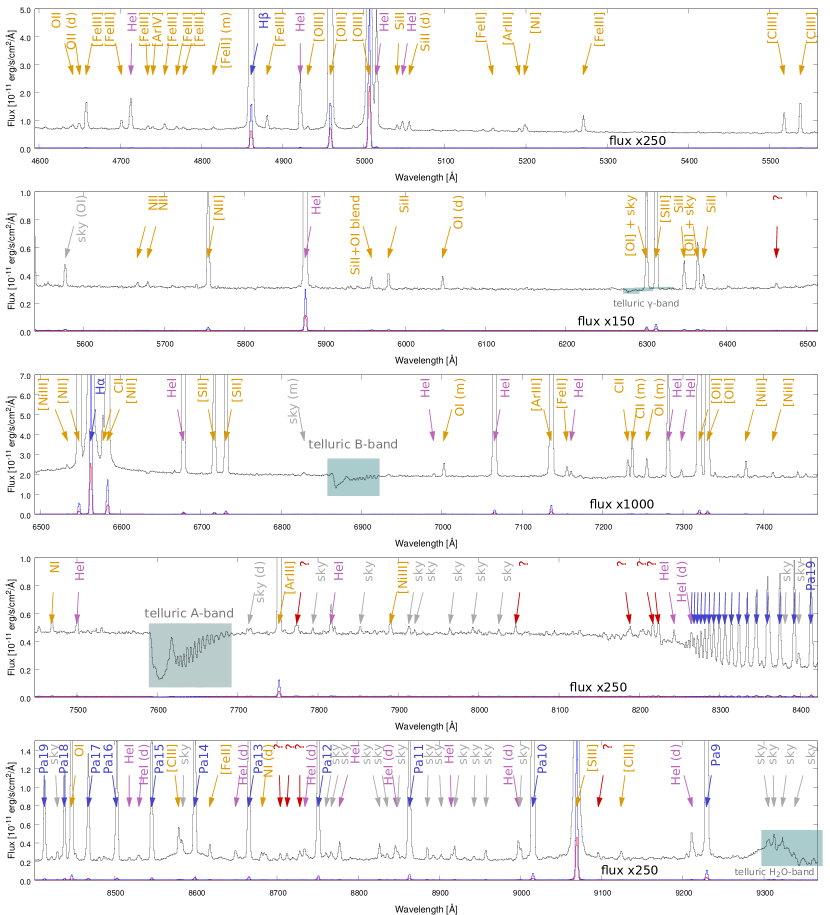
Figure 14: Full spectrum of the MUSE dataset, extracted at the approximate positions of slit1 of Baldwin et al. (1991) (red) and at the optical slit of Osterbrock et al. (1992) (blue). The “slit1”-spectrum is shown again in black, multiplied with the factor at the bottom of each panel, to highlight fainter lines. Note that the different panels have different absolute scales. Line identifications from the same two references are shown, hydrogen lines are in blue (lines Pa20 to Pa35 are marked but not annotated), helium lines in violet, metal lines in orange, and lines where the sky contribution dominates are grey. Unresolved line doublets and multiplets are marked with ’(d)’ and ’(m)’, respectively. A few faint lines without identification are marked in red.

Fig. 14 presents two nebular spectra over the full wavelength range extracted from the MUSE data. At the blue end of the spectrum, the first visible emission line is O ii 4642, but in the cube, several other, even fainter lines are detected. Hydrogen Paschen lines can be discriminated from Pa9 to Pa35 at the red end.

Like the extraction regions from the cube, the line identification in Fig. 14 were taken from Baldwin et al. (1991) and Osterbrock et al. (1992). We can identify lines down to a flux of about $0.005\times F_{\mathrm{{He\textsc{i}}6678}}$ listed in their reference tables. However, a few lines visible in our spectrum are not listed in these reference sources and are not known sky emission lines. They remain unidentified and are specially marked in our figure.

As a first demonstration of what is possible with this new dataset, we analyze the nebular emission in a spatially resolved (pixel by pixel) manner.

5.1 Extinction

We follow O’Dell & Harris (2010) by selecting an intrinsic H$\alpha$ to H$\beta$ flux ratio of 2.89, for case B and $T_{e}=9000$ K (see Storey & Hummer, 1995; Osterbrock & Ferland, 2005). We interpolate the flux measurement of the Balmer lines at the positions of bright stars (where the Balmer decrement could not be measured reliably), and then input them as well as the reference value into the PyNeb software (v1.0.9, Luridiana et al., 2013, 2015), and derive a reddening map using the extinction curve of Cardelli et al. (1989) as refined for the Orion Nebula by Blagrave et al. (2007) with $R_{V}=5.5$. This map is displayed in Fig. 15 as $c_{\mathrm{H\beta}}$. The contour levels displayed there correspond to $0.9\lesssim A_{V}\lesssim 2.7$ mag or – when applying the relation of Bohlin et al. (1978) – to column densities of $9.6\times 10^{20}\lesssim N(\mathrm{HI}+\mathrm{H}_{2})\lesssim 2.9\times 10^{21}\,\mathrm{cm}^{-2}$. As expected, the regions of the “Dark Bay” and the SW cloud (O’Dell et al., 2009) show the strongest extinction while e. g. the region south-east of the “Bright Bar” as well as the western arc-minute of our field exhibit very moderate reddening. By contrast with (sub)millimeter emission maps (e. g. Johnstone & Bally, 1999), the foreground dust structure appears smooth and devoid of significant substructure. Such substructure is most commonly seen in self-gravitating gas clouds that form filamentary and clumpy structures on scales from the parent cloud down to individual protostars (e. g. Johnstone & Bally, 2006; Takahashi et al., 2013). The lack of this clumping in our extinction map suggests that this foreground material is not self-gravitating.

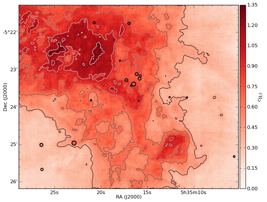
Figure 15: Extinction map of the central Orion Nebula, as derived from the H$\alpha$ to H$\beta$ flux ratio, displayed as $c_{\mathrm{H\beta}}$. Bright stars are marked again with black circles, the smoothed contours are $0.4\leq c_{\mathrm{H\beta}}\leq 1.2$ in steps of 0.2.

While qualitatively similar to the reddening map derived by O’Dell & Yusef-Zadeh (2000) from a radio-to-optical surface brightness comparison we note that we only reach peak values of $c_{\mathrm{H\beta}}=1.35$ in the Dark Bay, whereas O’Dell & Yusef-Zadeh found values up to 2.0. The comparison to their Balmer decrement-derived map, however, shows very similar absolute trends over the smaller area covered by them, such that in the vicinity of the Trapezium $c_{\mathrm{H\beta}}$ reaches 0.8 but is only about 0.5 between the SW cloud and the Trapezium.

We use this map to correct all measured emission line fluxes for reddening. We then also use the extinction-corrected flux maps to recreate a ”dust-free” version of Fig. 13 in Fig. 13 as well as Fig. 13 (for which no uncorrected counterpart is shown). It is apparent from the latter image that the reddening correction based on the Balmer-decrement is imperfect, since the Dark Bay and the SW cloud get more transparent but do not disappear.

5.2 Emission line maps

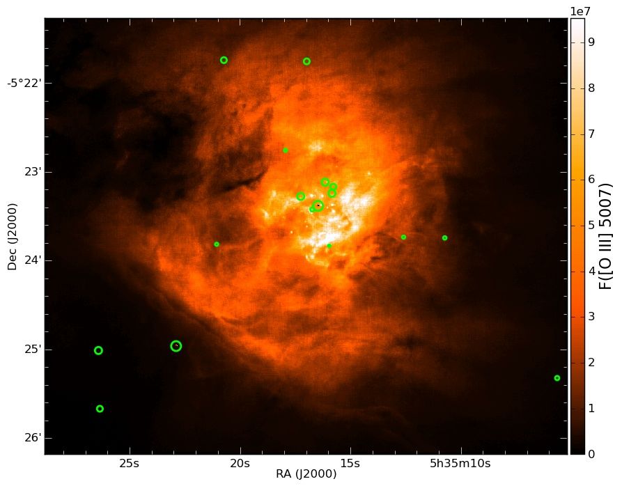
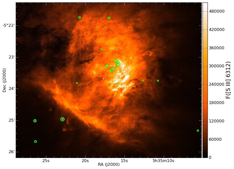
Figure 16: Reddening-corrected flux map of [O iii] 5007.

Figure 17: Reddening-corrected flux map of [S iii] 6312.

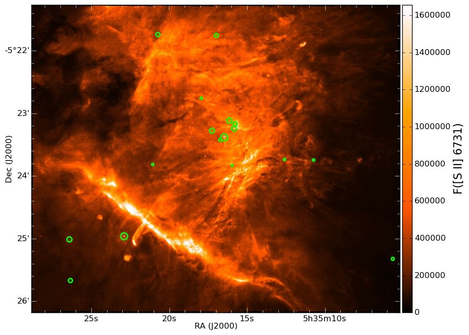
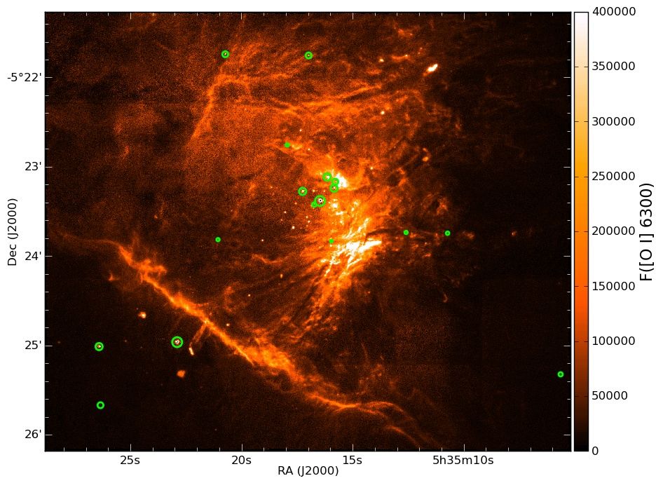
Figure 18: Reddening-corrected flux map of [S ii] 6731.

Figure 19: Reddening-corrected flux map of [O i] 6300, partially corrected for sky-line contribution.

Figures 19 to 19 show the Orion Nebula in dedicated emission lines as representatives of different ionization stages. The images of the Orion Nebula are more compact and diffuse in the higher ionized lines [O iii] 5007 and [S iii] 6312 than in the lower ionized lines [S ii] 6731 and [O i] 6300.

The fact that the images in the low ionization lines such as [O i] are much more structured than in the higher ionization lines is caused by the fact that the low ionization lines only form over a very narrow range of physical conditions in the nebula in comparison to the high ionization lines. Such effects are known e. g. from images of planetary nebulae taken in the light of different emission lines (Osterbrock & Ferland, 2005). Neutral gas is also often intrinsically more structured as the lower temperature, and therefore pressure, means that the neutral gas is more easily compressed.

5.3 Diagnostic maps

With the amount of emission lines present in the MUSE data and the reddening correction derived in Sect. 5.1, we can easily create flux ratio images, i. e. diagnostic maps.

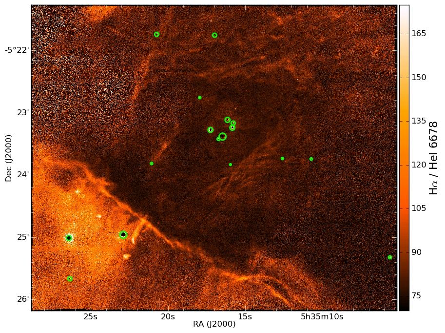
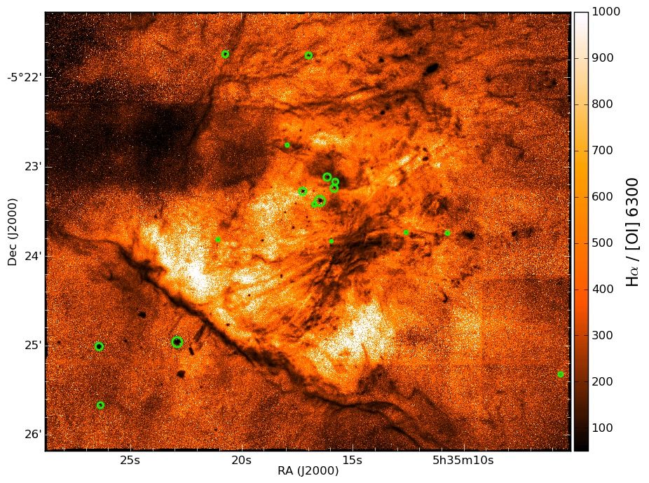
Figure 20: Reddening-corrected emission line ratio map of H$\alpha$/He i 6678.

Figure 21: Reddening-corrected emission line ratio map of H$\alpha$/[O i] 6300, partially corrected for sky-line contribution to [O i] 6300.

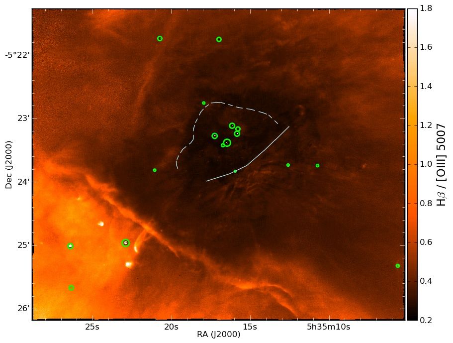
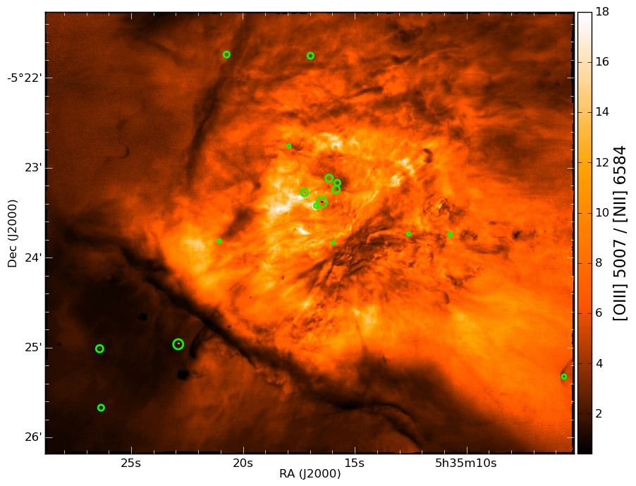
Figure 22: Reddening-corrected emission line ratio map of H$\beta$/[O iii] 5007. The [O iii] shell and the SE-NW ionization boundary discussed by O’Dell et al. (2009) are marked.

Figure 23: Reddening-corrected emission line ratio map of [O iii] 5007/[N ii] 6584.

The diagnostic images (Fig. 23 to 23) – based on different line intensity ratios – highlight different regions in the Orion nebula. The figures based on the H$\alpha$/He i 6678 (Fig. 23) and H$\beta$/[O iii] 5007 (Fig. 23) line ratios highlight the innermost and most strongly ionized structures of the nebula surrounding the central Trapezium stars. These line ratios are mainly indicators of the mean level of ionization and temperature (Osterbrock & Ferland, 2005). The discovery of a central [O iii] shell surrounding the Trapezium stars has been reported by O’Dell et al. (2009), indicating a stationary high-ionization structure. We also see hints of this structure in our H$\beta$/[O iii] 5007 image (Fig. 23, cf. Fig. 3 of O’Dell et al. 2009) and may even detect this H$\alpha$/He i 6678 map (Fig. 23). Furthermore, extended shell structures are clearly visible towards the north.

In the [O iii] 5007/[N ii] 6584 image (Fig. 23) the darker Orion-S region stands out south-west of the Trapezium. This foreground Orion-S complex hosts embedded stars that are sources of many large-scale optical outflows (O’Dell et al., 2009). The bright elongated region towards the outer south-west highlights the shocked wind region. Here the gas flows towards the low-density end in a so-called champagne flow (Arthur & Hoare, 2006). In addition, the bow shock connected to the T-Tauri star LL Ori (see spectrum in Fig. 3) sticks out to the outermost southwest. Furthermore, towards the west a loop structure pops up. Similar structures can be recognized as well in highly processed 20 cm-continuum images taken with the VLA (Yusef-Zadeh, 1990).

The H$\alpha$/[O i] 6300 image (Fig. 23) shows sharp extended structures in the outer (cooler) regions of the Orion Nebula.

5.4 Electron temperature / density

We again use PyNeb to cross-iterate electron density ($N_{\mathrm{e}}$) and electron temparature ($T_{\mathrm{e}}$) of the ionized gas, using extinction-corrected line ratios. We use the temperature sensitive line ratios [N ii] 5755/6548, [N ii] 5755/6584, and [S iii] 6312/9069 together with the density sensitive ratios [S ii] 6731/6716 and [Cl iii] 5538/5518, and let the iteration start at $T_{\mathrm{e}}=10000$ K. The assumptions for using PyNeb are, that the $n$-level approximation that this tool is based on (also see De Robertis et al., 1987, for a 5-level precursor) can describe the ionized states of the gas involved, and that the gas along the line of sight is sufficiently homogeneous for the emission lines to represent the luninosity-weighted physical state of the ionized gas in each spatial element.

We derive maps of $T_{\mathrm{e}}$ from [N ii] (averaged from 5755/6548 and 5755/6584, cross-iterated with [S ii]) and [S iii] 6312/9069 (cross-iterated with [S ii] ), and $N_{\mathrm{e}}$ from [S ii] 6731/6716 and [Cl iii] 5538/5518.

Since we did not attempt to disentangle stellar continuum and gas or mask positions of stars, many strong small-scale features in these maps may be artifacts. This can be easily verified using a continuum part of the spectral range. The brightest stars are therefore marked on the corresponding maps.

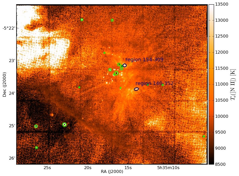
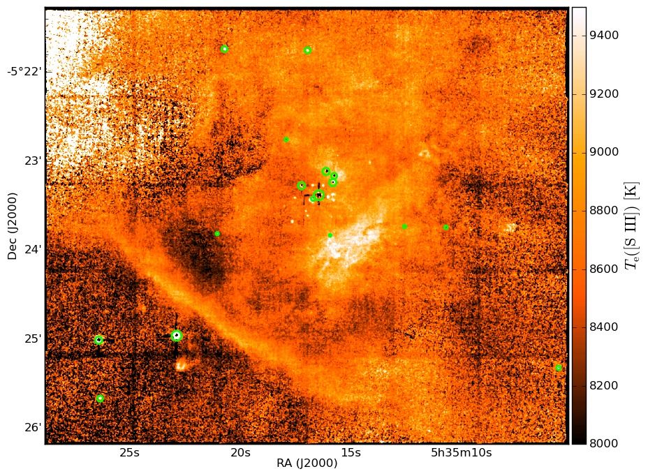
Figure 24: [N ii]-derived $T_{\mathrm{e}}$-map of the central Orion Nebula, smoothed by a median filter of 5$\times$5 pixels box width, displayed in linear scaling. See text for more details.

Figure 25: [S iii]-derived $T_{\mathrm{e}}$-map of the central Orion Nebula, smoothed by a median filter of 5$\times$5 pixels box width, displayed in linear scaling. See text for more details.

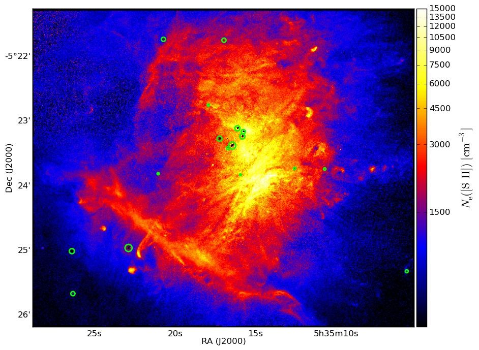
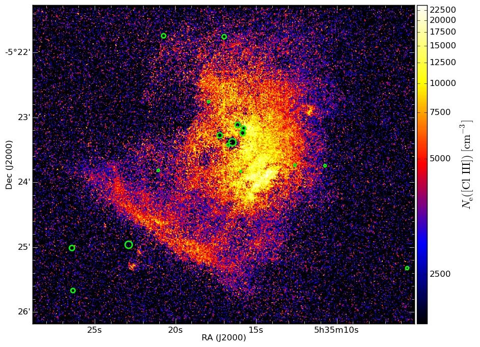
Figure 26: [S ii]-derived $N_{\mathrm{e}}$-map of the central Orion Nebula, smoothed by a median filter of 3$\times$3 pixels box width, displayed in asinh scaling. See text for more details.

Figure 27: [Cl iii]-derived $N_{\mathrm{e}}$-map of the central Orion Nebula, smoothed by a median filter of 5$\times$5 pixels box width, displayed in asinh scaling. See text for more details.

In the [N ii]-derived $T_{\mathrm{e}}$-map in Fig. 27, the hottest regions are 154-309 (in the coordinate system of O’Dell & Wen, 1994), about 21″ NW from $\theta^{1}$ Ori C (marked in Fig. 27), and 140-352, 47″ SW of $\theta^{1}$ Ori C, both reaching $\sim$13000 K. The coldest region appears to be beyond the Bright Bar, around $\theta^{2}$ Ori A and $\theta^{2}$ Ori B, with $T_{\mathrm{e}}\sim 8500$ K. That $T_{\mathrm{e}}$ is found to be high in the Dark Bay may be a problem of imperfect extinction correction. A grid-like pattern is visible in this map, caused by the $T_{\mathrm{e}}$ estimate to be about 200-300 K lower in the regions where multiple exposures overlap with adjacent pointings. This is caused by a slight systematic bias of the weaker line [N ii] 5755 and can be viewed as a represention the systematic uncertainty of these maps.

The [S iii]-derived $T_{\mathrm{e}}$-map in Fig. 27 shows a different behavior in comparison to the [N ii]-derived map. The hottest regions are some of the Herbig-Haro shocks, e. g. HH 204 reaching $\sim$9200 K, and the Bright Bar and the region SW (called the “Orion-S” feature by O’Dell et al., 2009) of the Trapezium are hotter than the surrounding nebula. The coldest regions in this ionization layer with about 7800 K are between the Bright Bar and the Dark Bay and between the Trapezium and the Dark Bay.

[S iii] was previously used by Foukal (1974) to derive $T_{\mathrm{e}}=9700\pm 1000$ K in a slit of $150\arcsec\times 15\arcsec$ in an unspecified location. Assuming that they pointed within the brightest part of the nebula but not on the Trapezium stars, their result agrees with ours. Again, the extremely high $T_{\mathrm{e}}$ values derived in the Dark Bay may be an artifact. Similar to $T_{\mathrm{e}}([{N\textsc{ii}}])$, the grid-like structure originates in the flux measurement of the fainter line [S iii] 6312.

Due to the density of known sources in the Orion Nebula and changes of the absolute world coordinate systems used in the literature, it is not always clear which known objects are related to features in our data. However, at least a few of the compact high-$T_{\mathrm{e}}$ peaks visible in Fig. 27 and 27 around the location of the Trapezium cluster can be identified with known young stellar objects and proplyds, e. g. 170-337 (O’Dell & Wen, 1994), d141-301 and j177-341 (Bally et al., 2000).

The electron density as derived using the [S ii] doublet (see Fig. 27) is consistent with the map derived by Pogge et al. (1992), but shows features with higher spatial resolution. $N_{\mathrm{e}}$ varies between $\sim 500\,\mathrm{cm}^{-3}$ at the edge of the field and densities in excess of $10\,000\,\mathrm{cm}^{-3}$ in the Orion-S region.

The layer of the ionization front showing [Cl iii] emission has an even higher density, reaching up to $N_{\mathrm{e}}\approx 25\,000\,\mathrm{cm}^{-3}$ in parts of the Orion-S region, as shown on Fig. 27. The lowest values derived from the [Cl iii] doublet give $N_{\mathrm{e}}\approx 4000\,\mathrm{cm}^{-3}$, just north of the Bright Bar. That $N_{\mathrm{e}}$ estimated from [Cl iii] gives higher densities than derived from [S ii] was qualitatively already presented by Núñez-Díaz et al. (2013). However, their scale does not allow a direct comparison to our map. For most of the field of view, the densities from [Cl iii] are too noisy to distinguish more than genereral trends with position.

The range in derived electron temperatures and densities prompted Sánchez et al. (2007) to compute the extinction values at each position using the physical gas conditions inferred by them. However, the dependency of the Case B Balmer decrement on the densities is weak (for the values derived here, it only changes by 1%). Since the temperature estimate is not independent of the reddening correction, we would need to add another layer of iterations. The expected changes are small (changes of the derived Balmer decrement reference value are at most 3%), we therefore prefer to not carry the analysis beyond this point.

5.5 Velocity field

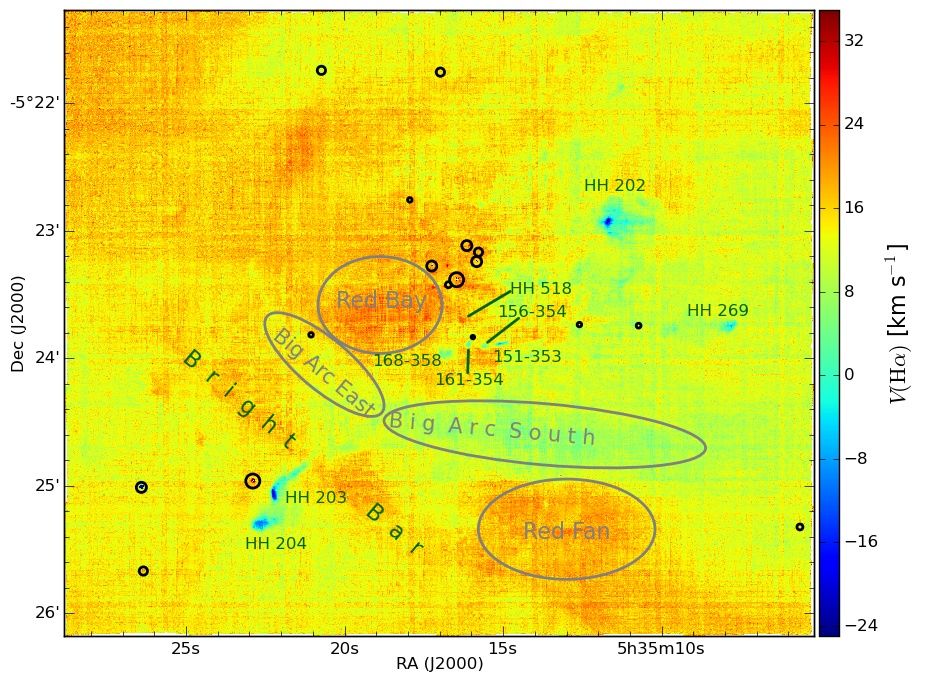
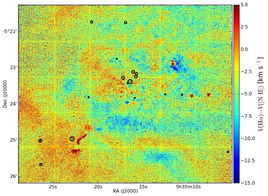
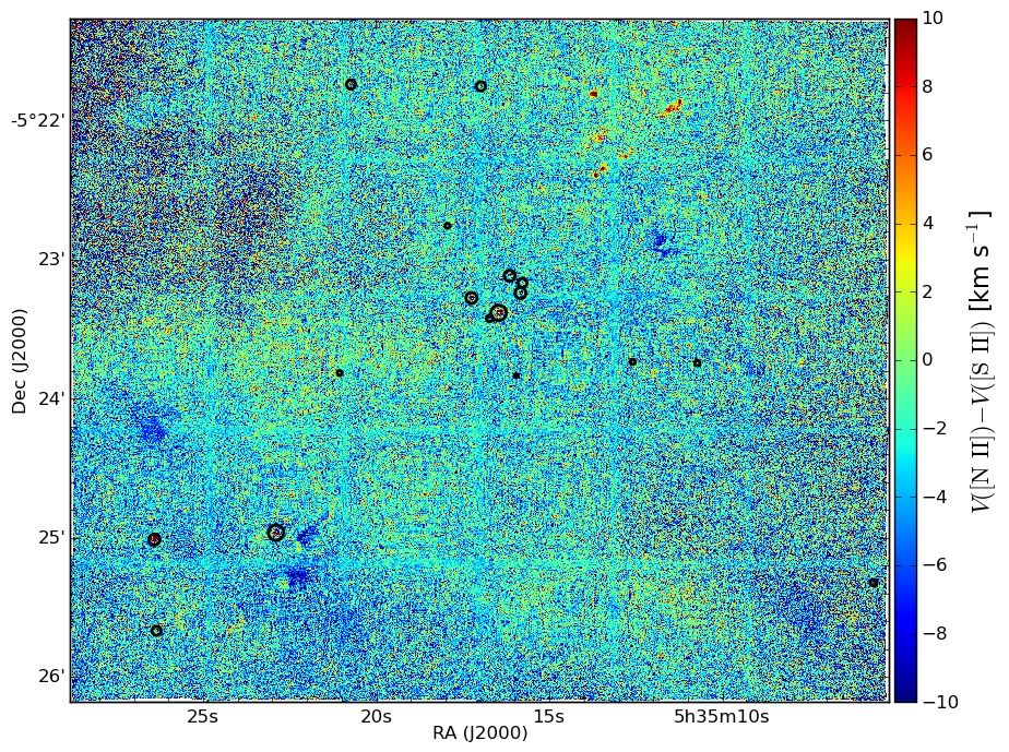
Figure 28: Velocity field as traced by the lines H$\alpha$ (top, with respect to barycentric velocity), [N ii] 6584 relative to H$\alpha$ (middle), and [S ii] 6731 relative to [N ii] 6584 (bottom). Note that the linear color scales are different for all these plots and that the range of the middle plot is asymmetric. The locations of the brighter stars in the field are marked as black circles, further noticeable features are annotated or marked in green or gray on the H$\alpha$ velocity map.

Fig. 28 shows the velocity field recovered from Gaussian centroids of the emission lines H$\alpha$ (absolute velocities against barycentric zeropoint), [N ii] 6584 (relative to H$\alpha$), and [S ii] 6731 (relative to [N ii]) for the full field mapped by MUSE.

The strongest features in velocity space for H$\alpha$ are the Herbig-Haro jets, especially the blueshifted objects HH 202, HH 269, HH 203, and HH 204 (marked on the H$\alpha$ velocity image in Fig. 28, top panel). A few more small-scale features are visible just south of the Trapezium stars, using the coordinate-based designation system for M 42 as invented by O’Dell & Wen (1994). The Bright Bar is visible as region of slightly enhanced velocity; more regions of visibly different redshift are marked with annotated grey ellipses on the H$\alpha$ velocity map of Fig. 28. The two higher velocity ($17\lesssim v_{\mathrm{H\alpha}}\lesssim 21$ km s^-1) regions were discussed by García-Díaz & Henney (2007), they were named ”Red Bay” for the region east of the Trapezium, and ”Red Fan” for the part just north of the western end of the Bright Bar. The elongated structure of lower velocities between Red Bay, Bright Bar, and Red Fan was discussed before in Doi et al. (2004) and named ”Big Arc” with a less pronounced eastern component ($11\lesssim v_{\mathrm{H\alpha}}\lesssim 14$ km s^-1 in our data) and a stronger and longer southern part ($3\lesssim v_{\mathrm{H\alpha}}\lesssim 14$ km s^-1 in the MUSE data). This map can be compared to the H$\alpha$ velocity map shown by García-Díaz et al. (2008, their Fig. 13). In both datasets, the large scale features show up in a very similar way. Even smaller features, like the velocity dips south of the Trapezium (especially at 168-358 and 161-354) are visibly similar. The absolute velocity values are slightly different between our data and theirs, with their value $\sim 2.5$ km s^-1 higher. This difference is within the combined error estimates of both datasets.

To highlight differences in velocity derived from our data for different ions, we also show the velocities derived for [N ii] 6584, subtracted from the H$\alpha$ velocity field (Fig. 28, middle panel). The velocity offset shown in this map is around $-3.5\pm 4.8$  km s^-1. Prominent features in this map are HH 202 to the west of the Trapezium and HH 203 and HH 204 beyond the Bright Bar, but on careful investigation it shows a plethora of other features, like blueshifted compact features not related to prominent Herbig-Haro objects, fainter filamentary structures around the Orion-S region and smoother large-scale changes. The Big Arc again shows up prominently, as blue region. Constructing the same velocity difference map from the data of García-Díaz et al. (2008) shows a very close match (W. Henney, priv. comm.). Their average velocity difference is $-3.7$ km s^-1 (their Table 2), very close to the value computed here, even though the area covered by their data is not identical.

The bottom panel of Fig. 28 shows the velocity difference map of [S ii] 6731 compared to [N ii] 6584. The velocity offset between these lines is much smaller, $-2.5\pm 4.8$  km s^-1. Large-scale features are less pronounced than in the previous velocity maps, and when interpreting them one should keep in mind that the scale shown is far below the velocity resolution achievable with MUSE. Nevertheless, the velocity differences beyond the Bright Bar, i. e. in the region around HH 203 and 204, seem systematically negative. We measure mean values of about $-4\,$ km s^-1 in that part of the nebula, so that the velocity of the [S ii] line is higher in that region than [N ii], in contrast to the central part where both lines appear to have similar velocities. Another possible velocity difference occurs within the Dark Bay, but the noise in that region is too large to be certain. This map can again be compared to the measurements of García-Díaz et al. (2008). Although their area is slightly smaller, they also find a comparable mean velocity difference of $-0.7$ km s^-1. In the velocity difference map created from their data, one can also determine values of zero in the Red Bay and the Red Fan, like in the MUSE data, but a slightly smaller difference beyond the Bright Bar ($-1.3$ km s^-1, W. Henney, priv. comm.). Small-scale features are again the well-known jets of HH 203 and HH 204 as well as HH 202. But here, some of the outflows from Orion-BN/KL as recently observed in the near-infrared by Bally et al. (2015) show up prominently as red patches to the north-west of the Trapezium, especially HH 201, HH 209, and features near HH 208.

6 Conclusions

We successfully demonstrated the capabilities of the integral-field spectrograph MUSE instrument with a new dataset representing imaging spectroscopy of the Huygens region of the Orion Nebula. The cubes we provide are among the largest 3D spectroscopic mosaics created so far. We showed that the MUSE data are of high quality in terms of positional accuracy, atmospheric refraction correction, $V$-band magnitude reconstruction, velocities, and flux calibration. We also pointed out artifacts in and imperfections of the data, and explained why two representations in cube form are necessary to cover all possible investigations.

The ensemble of data presented here already allows to investigate a variety of science topics. In this paper, we restricted ourselved to only give a demonstration, with a simple analysis of the ionized gas in the nebula. We derived the extinction towards the ionization front, and the electron temperature and density using two different emission line ratios, showing the physical properties in different layers of the warm gas around $\theta^{1}$ Ori C and the Trapezium cluster. Further analysis of this data will be presented in McLeod et al. (in prep.) where we will analyze structures and kinematics in the Orion Nebula.

Note that smart spatial binning of the existing MUSE data would enable detection weaker spectral features that in our pixel-by-pixel analysis are detected with sufficient S/N only in the central part. In the long term it might prove useful to re-observe the field with MUSE, with possibly a longer exposure time and/or more exposures per pointing, maybe mapping an even larger field. This would allow to estimate physical properties from fainter emission lines, and to map properties with even lower systematic effects to the outskirts of M 42.

Until that time, the current dataset is of high quality and already maps the most interesting area of the Orion Nebula in the optical wavelength range. It can serve as reference for many follow-up studies. To enable the widest possible use of these exceptional legacy data for science questions from members of the community, we publicly release the complete, reduced cubes as well as the inferred reddening, density, and temperature maps on http://muse-vlt.eu/science.