Strong three-meson couplings of $J/\psi$ and $\eta_{c}$

Abstract

We discuss the strong couplings $g_{PPV}$ and $g_{VVP}$ for vector ($V$) and pseudoscalar ($P$) mesons, at least one of which is a charmonium state $J/\psi$ or $\eta_{c}$. The strong couplings are obtained as residues at the poles of suitable form factors, calculated in a broad range of momentum transfers using a dispersion formulation of the relativistic constituent quark model. The form factors obtained in this approach satisfy all constraints known for these quantities in the heavy-quark limit. Our results suggest sizably higher values for the strong meson couplings than those reported in the literature from QCD sum rules.

1 Introduction

Strong couplings involving three mesons are complicated objects posing a great challenge for their theoretical study. The $D^{*}D\pi$ coupling, for which most theoretical analyses predicted values sizably smaller than the one later measured by CLEO cleo , illustrates this statement very well. In this letter, we address the strong three-meson couplings involving $J/\psi$ and $\eta_{c}$ states. These quantities cannot be measured directly in strong $J/\psi$ and $\eta_{c}$ decays, but they are important for our understanding of the $J/\psi$ and $\eta_{c}$ properties in a hadronic medium lin2000 .

Most results for charmonium couplings arose from rather detailed QCD sum-rule calculations bracco2005 ; matheus2005 ; bracco2014 ; bracco2015 . In the past, however, the application of QCD sum rules to three-meson couplings faced a great problem: QCD sum rules strongly underestimated the $D^{*}D\pi$ coupling (see, e.g., braun ) and the origin of this discrepancy has not been fully clarified. We thus present an alternative analysis of the family of $J/\psi$ and $\eta_{c}$ couplings using the relativistic dispersion approach da , one of the approaches which managed to predict correctly the $D^{*}D\pi$ coupling mb ; ms before the CLEO measurement.

The strong couplings in the focus of our interest, $g_{PV^{\prime}V}$ and $g_{PP^{\prime}V},$ are defined by

$$\langle P^{\prime}(p_{2})V(q)|P(p_{1})\rangle =-\mbox{$\frac{1}{2}$}g_{PP^{\prime}V}(p_{1}+p_{2})^{\mu}\varepsilon^{*}_{\mu}(q),$$

$$\langle V^{\prime}(p_{2})V(q)|P(p_{1})\rangle =-\epsilon_{\varepsilon^{*}(q)\varepsilon^{*}(p_{2})p_{1}p_{2}}g_{PV^{\prime}V},$$ (1.1)

with momentum transfer $q=p_{1}-p_{2}$. Accordingly, $g_{PP^{\prime}V}$ is dimensionless whereas $g_{PV^{\prime}V}$ has inverse mass dimension.

These strong couplings are related to the residues of the poles in the transition form factors at time-like momentum transfer arising from contributions of intermediate meson states in the transition amplitudes’ $q^{2}$ channel. We study the form factors $F_{+}^{P\to P^{\prime}}(q^{2})$, $V^{P\to V}(q^{2})$, and $A_{0}^{P\to V}(q^{2}),$ related to the transition amplitudes induced by vector quark currents $\bar{q}_{2}\gamma_{\mu}q_{1}$ or axial-vector quark currents $\bar{q}_{2}\gamma_{\mu}\gamma_{5}q_{1}$:

$$\langle P^{\prime}(p_{2})|\bar{q}_{2}\gamma_{\mu}q_{1}|P(p_{1})\rangle =F_{+}^{P\to P^{\prime}}(q^{2})(p_{1}+p_{2})_{\mu}+\cdots,$$

$$\langle V(p_{2})|\bar{q}_{2}\gamma_{\mu}q_{1}|P(p_{1})\rangle =\frac{2V^{P\to V}(q^{2})}{M_{P}+M_{V}}\epsilon_{\mu\varepsilon^{*}(p_{2})p_{1}p_{2}},$$

$$\langle V(p_{2})|\bar{q}_{2}\gamma_{\mu}\gamma_{5}q_{1}|P(p_{1})\rangle ={\rm i}q_{\mu}(\varepsilon^{*}(p_{2})p_{1})\frac{2M_{V}}{q^{2}}A_{0}^{P\to V}(q^{2})+\cdots,$$

where dots stand for other Lorentz structures. The poles in the above form factors are of the form

$$F_{+}^{P\to P^{\prime}}(q^{2}) = \frac{g_{PP^{\prime}V_{R}}f_{V_{R}}}{2M_{V_{R}}}\frac{1}{1-q^{2}/M_{V_{R}}^{2}}+\cdots,$$

$$V^{P\to V}(q^{2}) = \frac{(M_{V}+M_{P})g_{PVV_{R}}f_{V_{R}}}{2M_{V_{R}}}\frac{1}{1-q^{2}/M^{2}_{V_{R}}}+\cdots,$$

$$A_{0}^{P\to V}(q^{2}) = \frac{g_{PP_{R}V}f_{P_{R}}}{2M_{V}}\frac{1}{1-q^{2}/M^{2}_{P_{R}}}+\cdots.$$ (1.2)

In these relations, $P_{R}$ and $V_{R}$ label pseudoscalar and vector resonances with appropriate quantum numbers; $f_{P}$ and $f_{V}$ are the leptonic decay constants of the pseudoscalar and vector mesons, respectively, defined in terms of the amplitude of the meson-to-vacuum transition induced by the axial-vector or vector quark currents according to

$$\langle 0|\bar{q}_{1}\gamma_{\mu}\gamma_{5}q_{2}|P(p)\rangle ={\rm i}f_{P}p_{\mu},$$

$$\langle 0|\bar{q}_{1}\gamma_{\mu}q_{2}|V(p)\rangle =f_{V}M_{V}\varepsilon_{\mu}(p).$$

2 Dispersion formulation of the relativistic constituent quark model

Relativistic constituent quark models cqm proved to constitute an efficient tool for the study of hadron properties, in particular of meson decay constants and transition form factors. An essential feature of the constituent quark picture is the appropriate matching of the quark currents in QCD ($\bar{q}\gamma_{\mu}q$, $\bar{q}\gamma_{\mu}\gamma_{5}q$, etc.) and the associated currents formulated in terms of constituent quarks ($\bar{Q}\gamma_{\mu}Q$, $\bar{Q}\gamma_{\mu}\gamma_{5}Q$, etc.). For light quarks, for instance, partial conservation of the axial-vector current requires the appearance of the pseudoscalar structure in the axial-vector current of the constituent quarks, similar to the case of the axial-vector current of the nucleon gv . For the currents containing heavy quarks, the matching conditions are simpler:

$$\bar{q}_{1}\gamma_{\mu}q_{2} =g_{V}\bar{Q}_{1}\gamma_{\mu}Q_{2}+\cdots,$$

$$\bar{q}_{1}\gamma_{\mu}\gamma_{5}q_{2} =g_{A}\bar{Q}_{1}\gamma_{\mu}\gamma_{5}Q_{2}+\cdots,$$

where the dots indicate contributions of other possible Lorentz structures gv . Constituent quarks $Q_{1}$ and $Q_{2}$ have masses $m_{1}$ and $m_{2}$, respectively. In general, the form factors $g_{V}$ and $g_{A}$ depend on the momentum transfer. Vector current conservation requires $g_{V}=1$ at zero momentum transfer for the elastic current and at zero recoil for the heavy-to-heavy quark transition. The specific values of the form factors $g_{V}$ and $g_{A}$ and their momentum dependences belong to the parameters of the model, as well as the quark masses and the wave functions of mesons regarded as relativistic quark–antiquark bound states. A relativistic treatment of two-particle contributions to the bound-state structure may be consistently formulated within a relativistic dispersion approach which takes into account only two-particle intermediate quark-antiquark states in Feynman diagrams anis . Such a formulation is explicitly relativistic-invariant: hadron observables like form factors or decay constants are given by spectral representations over the invariant masses of the quark-antiquark intermediate states. Application of the dispersion formulation of the constituent quark picture to heavy-to-light meson form factors has convincingly demonstrated the reliability of this approach ms .

2.1 Meson decay constants and form factors as spectral integrals

Within the dispersion formulation of the constituent quark model, the decay constants $f_{P}$ and $f_{V}$ of pseudoscalar and vector mesons are expressed in the form of relativistic spectral representations, over the invariant masses of the intermediate quark–antiquark states, of the spectral densities involving the nonperturbative meson wave functions $\phi_{P}(s)$ and $\phi_{V}(s),$ respectively da :

$$f_{P} = \sqrt{N_{c}}\int\limits_{(m_{1}+m)^{2}}^{\infty}{\rm d}s\,\phi_{P}(s)\,(m_{1}+m)\frac{\lambda^{1/2}(s,m_{1}^{2},m^{2})}{8\pi^{2}s}\frac{s-(m_{1}-m)^{2}}{s},$$

$$f_{V} = \sqrt{N_{c}}\int\limits_{(m_{1}+m)^{2}}^{\infty}{\rm d}s\,\phi_{V}(s)\,\frac{2\sqrt{s}+m_{1}+m}{3}\frac{\lambda^{1/2}(s,m_{1}^{2},m^{2})}{8\pi^{2}s}\frac{s-(m_{1}-m)^{2}}{s},$$ (2.3)

with $\lambda(a,b,c)\equiv(a+b-c)^{2}-4ab$. The wave functions $\phi_{i}(s)$, $i=P,V,$ can be written as

$$\phi_{i}(s)=\frac{\pi}{\sqrt{2}}\frac{\sqrt{s^{2}-(m_{1}^{2}-m^{2})^{2}}}{\sqrt{s-(m_{1}-m)^{2}}}\frac{w_{i}(k^{2})}{s^{3/4}},\qquad k^{2}=\frac{\lambda(s,m_{1}^{2},m^{2})}{4s},$$ (2.4)

with $w_{i}(k^{2})$ normalized according to

$$\int{\rm d}k\,k^{2}w^{2}_{i}(k^{2})=1.$$ (2.5)

Notice that Eqs. (2.1) may be rewritten as the Fourier transform of the meson relativistic wave function at the origin.

Similarly, the $M_{1}(p_{1})\to M_{2}(p_{2})$ transition form factors induced by the constituent-quark transition current $\bar{Q}_{1}\hat{O}Q_{2}$ in the kinematical region $-\infty<q^{2}\leq(m_{2}-m_{1})^{2}$ is given by the double spectral representation

$$F_{i}(q^{2})=\int{\rm d}s_{1}\,\phi_{1}(s_{1})\int{\rm d}s_{2}\,\phi_{2}(s_{2})\,\Delta_{i}(s_{1},s_{2},q^{2}).$$ (2.6)

The function $\Delta_{i}(s_{1},s_{2},q^{2})$ is the double spectral density of the relevant Feynman diagrams with constituent quarks in the loop (Fig. 1). It contains the $\theta$-functions corresponding to the quark-antiquark thresholds and a specific constraint coming form the triangle Feynman diagram. The explicit expressions for $\Delta_{i}(s_{1},s_{2},q^{2})$ are given in Sect. 3.2 of da and will not be reproduced here. We point out that at $q^{2}<0$, the form factors obtained within the dispersion formulation are equal to the form factors of the light-front relativistic constituent quark model (Ref. 3 in cqm ). Correspondingly, the double spectral representation (2.6) at $q^{2}<0$ may be rewritten as the convolution of the light-cone wave functions of the initial and the final hadrons (see Eq. (2.86) of da ), or, equivalently, as the Fourier transform in the transverse variables of the overlap of these wave functions. The merit of having explicitly relativistic-invariant spectral representations compared to other formulations is the possibility to obtain the form factors in the decay region $0<q^{2}\leq(m_{2}-m_{1})^{2}$ by the analytic continuation in $q^{2}$ which was shown to lead to the appearance of the anomalous cut melikhov . Noteworthy, both the normal and the anomalous contributions involve the $s_{1}$ and $s_{2}$ integrations over the corresponding two-particle cuts, i.e. for $k_{1}^{2}>0$ and $k_{2}^{2}>0$ with $k_{{}_{1},2}$ given by (2.4). As the result, the form factors in a broad kinematical region $-\infty<q^{2}\leq(m_{2}-m_{1})^{2}$ are expressed in terms of the relativistic wave functions of the participating mesons $w_{1}(k_{1}^{2})$ and $w_{2}(k_{2}^{2})$ with $k_{1}^{2}>0$ and $k_{2}^{2}>0$. In this region, the precise form of the wave functions $w(k_{i}^{2})$ is not crucial; essential is only that the confinement effects have been taken into account. That is why, as shown in the applications to meson transition form factors ms , a simple Gaussian parameterization can be adopted:

$$w_{i}(k^{2})\propto\exp(-k^{2}/2\beta_{i}^{2}).$$ (2.7)

The spectral representation (2.6) is based on constituent-quark degrees of freedom and we apply it to calculate the form factors in the region $q^{2}<(m_{2}-m_{1})^{2}$. We then numerically interpolate the results of our calculations and use the obtained parameterizations to study the form factors at $q^{2}>(m_{1}-m_{2})^{2}$, where one expects the appearance of meson resonance at $q^{2}=M_{R}^{2}$.

The use of the dispersion formulation of the constituent quark model allows us to reveal the intimate connection between different decay modes and to perform the calculations in the broad range of $q^{2}$ which includes the scattering region $q^{2}<0$ and the physical region of the quark weak decay $0<q^{2}<(m_{2}-m_{1})^{2}$. In fact, quark models are the only approach that leads to relations between the decays of different mesons through the meson wave functions and provides the form factors in the $q^{2}$-range indicated above. It is important to emphasize that the form factors (2.6) reproduce correctly the structure of the heavy-quark expansion in QCD for heavy-to-heavy and heavy-to-light transitions if the radial wave functions $w_{i}(k^{2})$ are localized in a region of the order of the confinement scale $\Lambda,$ i.e., $k^{2}\leq\Lambda^{2}$ melikhov .

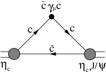
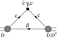
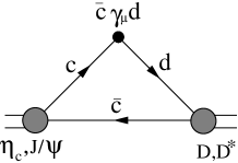
(a)	(b)	(c)

Fig. 1: Feynman diagrams for the transitions under consideration induced by the quark vector currents $\bar{Q}\gamma_{\mu}Q$: (a) $\eta_{c}\to\eta_{c},J/\psi$ induced by the current $\bar{c}\gamma_{\mu}c,$ (b) $D\to D,D^{*}$ induced by the current $\bar{c}\gamma_{\mu}c,$ and (c) $\eta_{c},J/\psi\to D,D^{*}$ induced by the current $\bar{c}\gamma_{\mu}d.$

2.2 Parameters of the model

For the wave functions, we make use of the simple Gaussian wave-function Ansatz which satisfies the localization requirement for $\beta\simeq\Lambda_{\rm QCD}$ and proved to provide a reliable picture of a large class of transition form factors ms .

Noteworthy, the quark-model double spectral representations take into account long-range QCD effects but not the short-range perturbative corrections. However, the parameters of the model (quark masses and nonperturbative meson wave functions corresponding to the choice of the constituent-quark couplings $g_{V}=1$ and $g_{A}=1$) are assumed such that our dispersion approach reproduces the observables (decay constants and some “well-measured” form factors from lattice QCD); therefore, radiative corrections to the quark propagators and to the vertices at the moderate momentum transfers considered are effectively taken care of by the use of constituent quark masses and the meson wave functions.

We employ the same values of the constituent quark masses and the quark couplings that have been obtained in ms :

$$g_{V}=g_{A}=1,\qquad m_{d}=m_{u}=0.23\;{\rm GeV},\qquad m_{s}=0.35\;{\rm GeV},\qquad m_{c}=1.45\;{\rm GeV}.$$ (2.8)

With the above quark couplings and masses, and the meson wave-function parameters $\beta$ collected in Table 1, the decay constants from our dispersion approach reproduce the best-known decay constants of pseudoscalar and vector mesons, also summarized in Table 1.

Table 1: Masses pdg , leptonic decay constants and corresponding wave-function parameters $\beta$ of charmed mesons and charmonia.

	$D$	$D^{*}$	$D_{s}$	$D_{s}^{*}$	$\eta_{c}$	$J/\psi$
$M$ (GeV)	$1.87$	$2.010$	$1.97$	$2.11$	$2.980$	$3.097$
$f$ (MeV)	$206\pm 8$ lmsfD ; pdg	$260\pm 10$ lmsfD* ; fDDs*lat	$248\pm 2.5$ fetac_lat	$311\pm 9$ fpsi_lat	$394.7\pm 2.4$ fetac_lat	$405\pm 7$ fpsi_lat ; pdg
$\beta$ (GeV)	$0.475$	$0.48$	$0.545$	$0.54$	$0.77$	$0.68$

Using the parameter values (2.8) and Table 1, the spectral representations (2.6) yield the form factors numerically. We then interpolate our numerical results by a simple physically motivated formula

$$F(q^{2})=\frac{F(0)}{\left(1-q^{2}/M_{R}^{2}\right)\left(1-\sigma_{1}q^{2}/M_{R}^{2}+\sigma_{2}q^{4}/M_{R}^{4}\right)},$$ (2.9)

where $M_{R}=M_{V}$ for $F_{+}$ and $V,$ and $M_{R}=M_{P}$ for $A_{0}$. We may use the parameters $F(0)$, $\sigma_{1,2}$ and $M_{R}$ as parameters of our fitting procedures. It turns out that for all form factors considered in this work, the value of $M_{R}$ obtained by the fit turns out to be very close (within few percent accuracy) to the mass of the resonance with the appropriate quantum numbers. This property opens the possibility to use the obtained parameterization (2.9) up to $q^{2}=M_{R}^{2}$ and to estimate the pole residues. In what follows we set $M_{R}$ equal to the known mass of the physical resonance and use the remaining parameters $F(0)$ and $\sigma_{1,2}$ as parameters of the fit. The parameters in (2.9) are related to the pole residue via

$${\rm Res}\,F(q^{2}=M_{R}^{2})=\frac{F(0)}{1-\sigma_{1}+\sigma_{2}}.$$ (2.10)

The residue is given by products of the (known) weak and the strong couplings $g$ to be determined. Finally, our fit parameters are $F(0)$, $\sigma_{1},$ and the strong coupling $g$ related to ${\rm Res}\,F(q^{2}=M_{R}^{2})$. In some cases, the residues of different form factors involve the same strong coupling; for such form-factor sets a constrained interpolation will be done.

3 The $\eta_{c}\eta_{c}J/\psi$ and $\eta_{c}J/\psi J/\psi$ strong couplings

The double spectral representations enable us to calculate the necessary form factors as soon as the vertex functions of the $\eta_{c}$ and $J/\psi$ are given. We fix the wave-function slope parameters $\beta_{i}$ such that the decay constants of $\eta_{c}$ and $J/\psi$ are reproduced by the spectral representations (2.1). Using for $\eta_{c}$ the lattice finding $f_{\eta_{c}}=(394.7\pm 2.4)\;\mbox{MeV}$ fetac_lat and for $J/\psi$ the experimental result $f_{\psi}=(407\pm 5)\;\mbox{MeV}$ pdg — which agrees excellently with the lattice determination $f_{\psi}=(405\pm 6\pm 2)\;\mbox{MeV}$ fpsi_lat — yields the wave-function parameters $\beta_{\eta_{c}}=0.77$ GeV and $\beta_{\psi}=0.68$ GeV. As soon as these are fixed, we calculate the form factors $F_{+}(\eta_{c}\to\eta_{c}),$ $V(\eta_{c}\to\psi),$ and $A_{0}(\eta_{c}\to\psi)$ in the kinematical region $q^{2}<0$ by using the dispersion representations (2.6).

The $\eta_{c}$ elastic form factor is normalized to $F^{\eta_{c}\to\eta_{c}}_{+}(0)=1$ by elastic vector-current conservation. Our determination of the $\psi\to\eta_{c}$ transition form factor $V^{\eta_{c}\to\psi}(0)=1.80$, describing the $\psi\to\eta_{c}\gamma$ radiative transition, is in reasonable agreement with both the data V(0)exp and the lattice-QCD result V(0)lat , in spite of some tension between these two findings: $V^{\rm exp}(0)=1.68\pm 0.14$ vs. $V^{\rm lat}(0)=1.92\pm 0.03\pm 0.02$. N.B.: In the limit $m_{c}\to\infty$, the heavy-quarkonium transition form factor approaches the value $V(0)=2$.

Next, we interpolate the results of our form-factor calculations performed for $-M^{2}_{\psi}<q^{2}<0$, by the fit formula (2.9). The residues of the form factors $F_{+}(\eta_{c}\to\eta_{c})$ and $A_{0}(\eta_{c}\to\psi)$ are given in terms of one and the same coupling $g_{\eta_{c}\eta_{c}\psi}$:

$${\rm Res}\;F_{+}(q^{2}=M_{\psi}^{2})=g_{\eta_{c}\eta_{c}\psi}f_{\psi}/2M_{\psi},\qquad{\rm Res}\;A_{0}(q^{2}=M_{\eta_{c}}^{2})=g_{\eta_{c}\eta_{c}\psi}f_{\eta_{c}}/2M_{\psi}.$$

Hence, we perform a combined fit to the two form factors $F_{+}(\eta_{c}\to\eta_{c})$ and $A_{0}(\eta_{c}\to\psi)$, regarding $g_{\eta_{c}\eta_{c}\psi}$, $A_{0}^{\eta_{c}\to\psi}(0)$ and the parameters $\sigma_{1}$ for $F_{+}(\eta_{c}\to\eta_{c})$ and $A_{0}(\eta_{c}\to\psi)$ as the fit parameters (recall that $F_{+}^{\eta_{c}\to\eta_{c}}(0)=1$ due to current conservation). The corresponding results are given in Table 2. These fits represent the numerical outcomes with a fantastic accuracy — better than 0.2% — in the full $q^{2}$ range considered. This lends strong support to the reliability of our approach to charmonia, in spite of the approximate form of our wave-function model.

The excellent description of our calculated form factors by the interpolation formula (2.9) suggests that this parameterization may be extended up to $q^{2}=M_{R}^{2}$ and used to calculate the strong couplings from the residue of the pole at $q^{2}=M_{R}^{2}$ in (2.9).

Table 2: Form factors describing the $\eta_{c}\to\eta_{c}$ and $\eta_{c}\to J/\psi$ transitions and corresponding strong couplings.

Amplitude	$\langle\eta_{c}|\bar{c}\gamma_{\mu}c|\eta_{c}\rangle$	$\langle J/\psi|\bar{c}\gamma_{\mu}\gamma_{5}c|\eta_{c}\rangle$	$\langle J/\psi|\bar{c}\gamma_{\mu}c|\eta_{c}\rangle$
Form factor	$F_{+}(\eta_{c}\to\eta_{c})$	$A_{0}(\eta_{c}\to J/\psi)$	$V(\eta_{c}\to J/\psi)$
$F(0)$	$1$	$0.900\pm 0.004$	$1.80\pm 0.01$
$M_{R}$	$M_{\psi}$	$M_{\eta_{c}}$	$M_{\psi}$
$\sigma_{1}$	$0.60\pm 0.01$	$0.77\pm 0.02$	$0.73\pm 0.04$
Strong coupling	$g_{\eta_{c}\eta_{c}\psi}=25.8\pm 1.7$		$g_{\eta_{c}\psi\psi}=(10.6\pm 1.5)\,{\rm GeV}^{-1}$

The statistical uncertainty reflects merely the accuracy of the description of the calculation outcomes by the fit formula, but does not take into account the systematic uncertainties related to the approximate character of the model and the specific form of the interpolating formula. The latter cannot be probed unambiguously. However, comparison with the results of the experiment or lattice QCD in those cases where these results are available, shows that the systematic uncertainty does not exceed the 10–15% level.

In the limit $m_{c}\to\infty$, we have $F_{+}(0)=1$ and $V(0)=2.$ Consequently, the strong couplings of heavy quarkonia satisfy $g_{\eta_{c}\eta_{c}\psi}=M_{\psi}g_{\eta_{c}\psi\psi},$ which is fulfilled with 20% accuracy for the charmonium couplings.

4 Strong couplings of $\eta_{c}$ and $J/\psi$ to $D$ and $D^{*}$

Here, the couplings of interest may be extracted from the residues of poles in form factors that describe two different kinds of transitions: transitions between the charmed mesons, induced by the currents $\bar{c}\gamma_{\mu}c$ and $\bar{c}\gamma_{\mu}\gamma_{5}c$ (Fig. 1b), and transitions between the charmonia and the charmed mesons, induced by the currents $\bar{c}\gamma_{\mu}d$ and $\bar{c}\gamma_{\mu}\gamma_{5}d$ (Fig. 1c). Our results for the form factors and the corresponding couplings are presented in Tables 4 and 4. Again, the small uncertainties of the obtained couplings do not reflect possible systematic errors related to the approximate nature of the dispersion approach.

Table 3: Strong couplings of $J/\psi$ to $D$ and $D^{*}$.

Amplitude	$\langle D|\bar{c}\gamma_{\mu}c|D\rangle$	$\langle J/\psi|\bar{c}\gamma_{\mu}\gamma_{5}d|D\rangle$	$\langle D^{*}|\bar{c}\gamma_{\mu}c|D\rangle$	$\langle J/\psi|\bar{c}\gamma_{\mu}d|D\rangle$
Form factor	$F_{+}(D\to D)$	$A_{0}(D\to\psi)$	$V(D\to D^{*})$	$V(D\to\psi)$
$F(0)$	$1$	$0.545\pm 0.003$	$1.186\pm 0.003$	$1.517\pm 0.003$
$M_{R}$	$M_{\psi}$	$M_{D}$	$M_{\psi}$	$M_{D^{*}}$
$\sigma_{1}$	$0.453\pm 0.017$	$0.58\pm 0.02$	$0.453\pm 0.013$	$0.59\pm 0.01$
Strong coupling	$g_{DD\psi}=26.04\pm 1.43$		$g_{DD^{*}\psi}=(10.71\pm 0.39)\;{\rm GeV}^{-1}$

Table 4: Strong couplings of $\eta_{c}$ to $D$ and $D^{*}$.

Amplitude	$\langle D|\bar{d}\gamma_{\mu}c|\eta_{c}\rangle$	$\langle D^{*}|\bar{d}\gamma_{\mu}\gamma_{5}c|\eta_{c}\rangle$	$\langle D^{*}|\bar{c}\gamma_{\mu}\gamma_{5}c|D\rangle$	$\langle D^{*}|\bar{d}\gamma_{\mu}c|\eta_{c}\rangle$
Form factor	$F_{+}(\eta_{c}\to D)$	$A_{0}(\eta_{c}\to D^{*})$	$A_{0}(D\to D^{*})$	$V(\eta_{c}\to D^{*})$
$F(0)$	$0.643\pm 0.002$	$0.491\pm 0.002$	$0.966\pm 0.004$	$1.503\pm 0.003$
$M_{R}$	$M_{D^{*}}$	$M_{D}$	$M_{\eta_{c}}$	$M_{D^{*}}$
$\sigma_{1}$	$0.466\pm 0.008$	$0.71\pm 0.01$	$0.39\pm 0.01$	$0.491\pm 0.008$
Strong coupling	$g_{DD^{*}\eta_{c}}=15.51\pm 0.45$			$g_{D^{*}D^{*}\eta_{c}}=(9.76\pm 0.32)\;{\rm GeV}^{-1}$

We emphasize that the excellent combined description of the sets of form factors involving the same strong coupling in their pole residues (with $\chi^{2}/{\rm DOF}\leq 0.1$ assigning a 1% error to our form-factor results) lends strong support to the reliability of our results. This is actually a highly nontrivial feature: for instance, the coupling $g_{DD^{*}\psi}$ is obtained from a combined description of $V(D\to D^{*})$ and $V(D\to\psi)$: the vector states here have completely different structure and properties and are described by rather different wave functions. Also the vector resonances that appear in the form factors at time-like momentum transfers differ: $J/\psi$ in $V(D\to D^{*})$ and $D^{*}$ in $V(D\to\psi)$. The excellent description of all sets of form factors strongly increases the reliability of our findings. The behavior of the “off-shell couplings” (viz., the suitably rescaled form factors equaling the strong couplings at $q^{2}=M_{R}^{2}$) is depicted in Fig. 2.

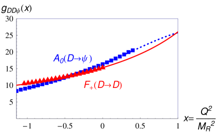
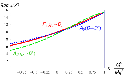
Fig. 2: The “off-shell” strong couplings. Left: $g_{D\hat{D}\psi}(x)=\frac{2M_{\psi}}{f_{D}}(1-x)A^{D\to\psi}_{0}(q^{2})$, $x=q^{2}/M_{D}^{2}$ (blue squares and blue dotted line), and $g_{DD\hat{\psi}}(x)=\frac{2M_{\psi}}{f_{\psi}}(1-x)F_{+}^{D\to D}(q^{2})$, $x=q^{2}/M^{2}_{\psi}$ (red triangles and red solid line), extracted from the form factors $A^{D\to\psi}_{0}(q^{2})$ and $F_{+}^{D\to D}(q^{2})$, respectively. Triangles and squares indicate the results computed numerically from the spectral representations, the dotted and solid lines the fits interpolating the results and then used for extrapolation to the pole regions. Right: $g_{D\hat{D^{*}}\psi}(x)$ obtained from $F_{+}^{\eta_{c}\to D}$ (red solid line); $g_{DD^{*}\hat{\psi}}(x)$ obtained from $A_{0}^{D\to D^{*}}$ (blue dotted line); $g_{\hat{D}D^{*}\psi}(x)$ obtained from $A_{0}^{D\to D^{*}}$ (green dashed line).

In the limit $m_{Q}\to\infty$, the form factors $F_{+}^{D\to D}(q^{2})$ and $V^{D\to D^{*}}(q^{2})$ are equal to each other. From (1), the coupling constants thus satisfy the heavy-quark symmetry relation $g_{DD\psi}=(M_{D}+M_{D}^{*})g_{DD^{*}\psi}$ — fulfilled with 30% accuracy.

5 Strong couplings of $\eta_{c}$ and $J/\psi$ to $D_{s}$ and $D_{s}^{*}$

The couplings of $J/\psi$ and $\eta_{c}$ to the charmed strange mesons $D_{s}$ and $D_{s}^{*}$ may be found from the residues of the form factors entering the transition amplitudes induced by the currents $\bar{c}\gamma_{\mu}c$, $\bar{c}\gamma_{\mu}\gamma_{5}c$, $\bar{d}\gamma_{\mu}c$ or $\bar{d}\gamma_{\mu}\gamma_{5}c$. The relevant Feynman diagrams may be inferred from those shown in Fig. 1a and Fig. 1b by replacing the $d$ quark by the $s$ quark. Tables 6 and 6 summarize the results of our analysis. Again, we emphasize the excellent simultaneous description of the sets of the form factors involving the same strong coupling in the pole residues.

Table 5: Strong couplings of $J/\psi$ to $D_{s}$ and $D_{s}^{*}$.

Amplitude	$\langle D_{s}|\bar{c}\gamma_{\mu}c|D_{s}\rangle$	$\langle J/\psi|\bar{c}\gamma_{\mu}\gamma_{5}s|D_{s}\rangle$	$\langle D_{s}^{*}|\bar{c}\gamma_{\mu}c|D_{s}\rangle$	$\langle J/\psi|\bar{c}\gamma_{\mu}s|D_{s}\rangle$
Form factor	$F_{+}(D_{s}\to D_{s})$	$A_{0}(D_{s}\to\psi)$	$V(D_{s}\to D_{s}^{*})$	$V(D_{s}\to\psi)$
$F(0)$	$1$	$0.630\pm 0.004$	$1.23\pm 0.01$	$1.67\pm 0.01$
$M_{R}$	$M_{\psi}$	$M_{D_{s}^{*}}$	$M_{\psi}$	$M_{D_{s}^{*}}$
$\sigma_{1}$	$0.39\pm 0.01$	$0.53\pm 0.01$	$0.39\pm 0.03$	$0.55\pm 0.02$
Strong coupling	$g_{D_{s}D_{s}\psi}=23.83\pm 0.78$		$g_{D_{s}D_{s}^{*}\psi}=(9.60\pm 0.80)\;{\rm GeV}^{-1}$

Table 6: Strong couplings of $\eta_{c}$ to $D_{s}$ and $D_{s}^{*}$.

Amplitude	$\langle D_{s}|\bar{s}\gamma_{\mu}c|\eta_{c}\rangle$	$\langle D_{s}^{*}|\bar{c}\gamma_{\mu}\gamma_{5}s|\eta_{c}\rangle$	$\langle D_{s}^{*}|\bar{c}\gamma_{\mu}\gamma_{5}c|D_{s}\rangle$	$\langle D_{s}^{*}|\bar{c}\gamma_{\mu}s|\eta_{c}\rangle$
Form factor	$F_{+}(\eta_{c}\to D_{s})$	$A_{0}(\eta_{c}\to D_{s}^{*})$	$A_{0}(D_{s}\to D_{s}^{*})$	$V(\eta_{c}\to D_{s}^{*})$
$F(0)$	$0.746\pm 0.002$	$0.576\pm 0.002$	$0.953\pm 0.004$	$1.66\pm 0.004$
$M_{R}$	$M_{D_{s}^{*}}$	$M_{D_{s}}$	$M_{\eta_{c}}$	$M_{D_{s}^{*}}$
$\sigma_{1}$	$0.42\pm 0.01$	$0.61\pm 0.01$	$0.35\pm 0.01$	$0.45\pm 0.01$
Strong coupling	$g_{D_{s}D_{s}^{*}\eta_{c}}=14.15\pm 0.52$			$g_{D_{s}^{*}D_{s}^{*}\eta_{c}}=(8.27\pm 0.37)\;{\rm GeV}^{-1}$

6 Summary and conclusions

We revisited the three-meson strong couplings involving $J/\psi$ and $\eta_{c}$ within the dispersion formulation of the relativistic constituent quark model. In this approach, various hadron observables are given by relativistic spectral integrals in terms of spectral densities of the relevant Feynman diagrams and of relativistic hadron wave functions. The hadron observables from this approach satisfy all rigorous constraints emerging in QCD in the heavy-quark limit if the hadron wave functions are localized in a region of the order of the confinement radius. The basic parameters of the model, such as the effective constituent quark masses, have been determined before in a study ms of heavy-meson transition form factors. Following ms , we fix the wave-function parameters of $J/\psi$, $\eta_{c}$, and the charmed and charmed strange mesons using the known results for the leptonic decay constants of these mesons. With these parameters at hand, the form factors of interest are calculated in the space-like region and the weak-decay region using relativistic dispersion integrals.

Our results may be summarized as follows:

1. As the dispersion integrals (2.6) are based on quark degrees of freedom, all our calculations are carried out far from the pole at $q^{2}=M_{R}^{2}$. However, the numerical interpolation formulas turn out to be excellently compatible with the pole at $q^{2}=M_{R}^{2}$ and therefore can be used up to $q^{2}=M_{R}^{2}$. This feature allows us to extract the residues of these form factors at $q^{2}=M_{R}^{2}$ and to derive in this way the three-meson couplings. We perform a combined analysis of groups of form factors involving the same strong couplings in the pole residues. In all cases we arrive at an excellent combined description of these form factors (that is, with $\chi^{2}/{\rm DOF}\leq 0.1$, assigning just a 1% error to our form-factor results). This is a highly nontrivial feature, as the same value of the strong coupling is extracted from form factors involving mesons which have entirely different wave functions. Such excellent description of all sets of form factors gives strong support to the credibility of our findings.

As summary of our predictions, we report,

• for the couplings involving $J/\psi$ and $\eta_{c}$ mesons,

  $$g_{\eta_{c}\eta_{c}\psi}=25.8\pm 1.7,$$

  $$g_{\eta_{c}\psi\psi}=(10.6\pm 1.5)\;{\rm GeV}^{-1},$$

• for the $J/\psi$ and $\eta_{c}$ couplings to charmed mesons,

  $$g_{DD\psi}=26.04\pm 1.43,$$

  $$g_{DD^{*}\psi}=(10.7\pm 0.4)\;{\rm GeV}^{-1},$$

  $$g_{DD^{*}\eta_{c}}=15.51\pm 0.45,$$

  $$g_{D^{*}D^{*}\eta_{c}}=(9.76\pm 0.32)\;{\rm GeV}^{-1},$$

• and, for the $J/\psi$ and $\eta_{c}$ couplings to charmed strange mesons,

  $$g_{D_{s}D_{s}\psi}=23.83\pm 0.78,$$

  $$g_{D_{s}D_{s}^{*}\psi}=(9.6\pm 0.8)\;{\rm GeV}^{-1},$$

  $$g_{D_{s}D_{s}^{*}\eta_{c}}=14.15\pm 0.52,$$

  $$g_{D_{s}^{*}D_{s}^{*}\eta_{c}}=(8.27\pm 0.37)\;{\rm GeV}^{-1}.$$

The uncertainties quoted in these results are merely the statistical uncertainties related to the accuracy of the description of our results by the fit formulas. There are, of course, also systematic uncertainties related to the approximate nature of the dispersion approach to the form factors; these uncertainties are very difficult to estimate unambiguously. Comparison of the couplings predicted by the dispersion approach mb ; ms with the results from experiment cleo ; BaBar and lattice QCD g_lat in those cases where such results are available, allows us to expect the accuracy of our predictions to be not worse than 15–20%.

2. Our results considerably exceed the ones from QCD sum rules (see the comparison in Table 7). Both approaches follow the same strategy for extracting the strong couplings: the form factors are calculated in a kinematical region far away from the pole and are then extrapolated to the pole region in order to isolate the residue. The advantage of the dispersion approach for the problem under consideration is twofold: we predict the form factor in a broader range of $q^{2}$ and we consider $q^{2}$ values closer to the pole region than the region where QCD sum rules may be applied. Therefore, we need to extrapolate the form factors over much narrower regions of the momentum transfer and thus believe that the results of the dispersion approach are more reliable.

Table 7: Comparison of our strong-coupling predictions with earlier results from QCD sum rules. For consistency with definition (1), the $PPV$ couplings from matheus2005 and bracco2014 have been multiplied by a factor 2.

	$g_{DD\psi}$	$g_{DD^{*}\psi}$ (GeV-1)	$g_{D_{s}D_{s}\psi}$	$g_{D_{s}D_{s}^{*}\psi}$ (GeV-1)
This work	$26.04\pm 1.43$	$10.7\pm 0.4$	$23.83\pm 0.78$	$9.6\pm 0.8$
QCD sum rules	$11.6\pm 1.8$ matheus2005	$4.0\pm 0.6$ matheus2005	$11.96\pm 1.34$ bracco2014	$4.30\pm 1.53$ bracco2015

3. We also investigated the $SU(3)$-breaking effects in the strong couplings. The replacement of the light quark by the strange quark leads to the increase of the considered transition form factors and of the corresponding residues. At the same time, however, also the leptonic decay constants of the charmed strange mesons considerably exceed those of their non-strange counterparts. The three-meson strong couplings are derived as ratios of the form-factor residues and the leptonic decay constants, and, eventually, the replacement of the non-strange quark by the strange quark leads to a reduction of the three-meson couplings at the level of some $10\%.$ In contrast, QCD sum rules observe an enhancement of the three-meson couplings when the light quark is replaced by the strange one.

Acknowledgements. D. M. is grateful to Berthold Stech for interesting and stimulating discussions. S. S. thanks MIUR (Italy) for partial support under Contract No. PRIN 2010–2011.

References

- (1) S. Ahmed et al. (CLEO Collaboration), Phys. Rev. Lett. 87, 251801 (2001).
- (2) Z. Lin and C. M. Ko, Phys. Rev. C 62, 034903 (2000).
- (3) M. E. Bracco, M. Chiapparini, F. S. Navarra, and M. Nielsen, Phys. Lett. B 605, 326 (2005).
- (4) R. Mattheus et al., Int. J. Mod. Phys. E 14, 555 (2005).
- (5) B. Osorio Rodriguez, M. E. Bracco, and M. Chiapparini, Nucl. Phys. A 929, 143 (2014).
- (6) B. Osorio Rodriguez et al., Eur. Phys. J. A 51, 28 (2015).
- (7) V. M. Belyaev, V. M. Braun, A. Khodjamirian, and R. Rückl, Phys. Rev. D 51, 6177 (1995).
- (8) D. Melikhov, Eur. Phys. J. direct C4, 2 (2002) [arXiv:hep-ph/0110087].
- (9) D. Melikhov and M. Beyer, Phys. Lett. B 452, 121 (1999).
- (10) D. Melikhov and B. Stech, Phys. Rev. D 62, 014006 (2000).
- (11) A. Le Yaouanc, L. Oliver, S. Ono, O. Pene, and J.-C. Raynal, Phys. Rev. D 31, 137 (1985); Phys. Rev. Lett. 54, 506 (1985); W. Lucha, F. Schöberl, and D. Gromes, Phys. Rep. 200, 127 (1991); F. Cardarelli, E. Pace, G. Salmè, and S. Simula, Phys. Lett. B 357, 267 (1995); R. N. Faustov and V. O. Galkin, Z. Phys. C 66, 119 (1995); D. Ebert, R. N. Faustov, and V. O. Galkin, Phys. Lett. B 635, 93 (2006).
- (12) D. Melikhov and B. Stech, Phys. Rev. D 74, 034022 (2006); W. Lucha, D. Melikhov, and S. Simula, Phys. Rev. D 74, 054004 (2006).
- (13) V. V. Anisovich, D. I. Melikhov, and V. A. Nikonov, Phys. Rev. D 55, 2918 (1997); A. F. Krutov and V. E. Troitsky, JHEP 9910, 028 (1999).
- (14) D. Melikhov, Phys. Rev. D 53, 2460 (1996); 56, 7089 (1997).
- (15) M. S. Bhagwat, M. A. Pichowsky, C. D. Roberts, and P. C. Tandy, Phys. Rev. C 68, 015203 (2003); G. Eichmann, R. Alkofer, I. C. Clöet, A. Krassnigg, and C. D. Roberts, Phys. Rev. C 77, 042202 (2008); D. Melikhov and S. Simula, Eur. Phys. J. C 37, 437 (2004).
- (16) K. A. Olive et al. (Particle Data Group), Chin. Phys. C 38, 090001 (2014).
- (17) W. Lucha, D. Melikhov, and S. Simula, Phys. Lett. B 701, 82 (2011).
- (18) W. Lucha, D. Melikhov, and S. Simula, Phys. Lett. B 735, 12 (2014).
- (19) D. Bečirević et al., JHEP 1202, 042 (2012).
- (20) C. T. H. Davies, C. McNeile, E. Follana, G. P. Lepage, H. Na, and J. Shigemitsu, Phys. Rev. D 82, 114504 (2010).
- (21) G. C. Donald, C. T. H. Davies, R. J. Dowdall, E. Follana, K. Hornbostel, J. Koponen, G. P. Lepage, C. McNeile, Phys. Rev. D 86, 094501 (2012).
- (22) R. E. Mitchell et al. (CLEO Collaboration), Phys. Rev. Lett. 102, 011801 (2009).
- (23) D. Bečirević and F. Sanfilippo, JHEP 1301, 028 (2013).
- (24) J. P. Lees et al. (BaBar Collaboration), Phys. Rev. Lett. 111, 111801 (2013).
- (25) D. Bečirević and F. Sanfilippo, Phys. Lett. B 721, 94 (2013); J. M. Flynn et al., arXiv:1506.06413 [hep-lat].