Irreversibility and small-scale generation in 3D turbulent flows

Abstract

In three-dimensional turbulent flows energy is supplied at large scales and cascades down to the smallest scales where viscosity dominates. The flux of energy through scales implies the generation of small scales from larger ones, which is the fundamental reason for the irreversibility of the dynamics of turbulent flows. As we showed recently, this irreversibility manifests itself by an asymmetry of the probability distribution of the instantaneous power $p$ of the forces acting on fluid elements. In particular, the third moment of $p$ was found to be negative. Yet, a physical connection between the irreversibility manifested in the distribution of $p$ and the energy flux or small-scale generation in turbulence has not been established. Here, with analytical calculations and support from numerical simulations of fully developed turbulence, we connect the asymmetry in the power distribution, i.e., the negative value of $\langle p^{3}\rangle$, to the generation of small scales, or more precisely, to the amplification (stretching) of vorticity in turbulent flows. Our result is the first step towards a quantitative understanding of the origin of the irreversibility observed at the level of individual Lagrangian trajectories in turbulent flows.

I Introduction

The generation of small scales, or large velocity gradients, is one of the most striking physical phenomenon of 3-dimensional (3D) turbulent fluid flows, and is responsible for a flux of energy $\varepsilon$ from large to small scales. Remarkably, in the limit of very small viscosity or very large Reynolds number, the third moment of the longitudinal velocity difference between two points separated by a distance $x$, $\langle\Delta u(x)^{3}\rangle$, is related to the energy flux by the relation $\langle\Delta u(x)^{3}\rangle=-\frac{4}{5}\varepsilon x$, which is one of the very few exact results in turbulence theory Kolmogorov (1941). In elementary terms, two points are more likely to be pushed closer together (repelled) when their relative energy is large (small) Falkovich et al. (2001). This fundamental asymmetry persists all the way down to very small distances so the third moment of the velocity derivative $\partial_{x}u_{x}$ is negative: $\langle(\partial_{x}u_{x})^{3}\rangle\leq 0$. In fact, available data from experiments using hot-wire anemometry Batchelor and Townsend (1947); Townsend (1951) and from direct numerical simulations (DNS) have led to the conclusion that the normalized third moment of $\partial_{x}u_{x}$, i.e., the skewness, $S_{\partial_{x}u_{x}}\equiv\langle(\partial_{x}u_{x})^{3}\rangle/\langle(\partial_{x}u_{x})^{2}\rangle^{3/2}$, is negative and approximately $-0.5$, with at most a weak dependence on the Reynolds number Sreenivasan and Antonia (1997); Ishihara et al. (2007). In homogeneous isotropic flows, the seminal work of Betchov Betchov (1956) shows that the third moment of $\partial_{x}u_{x}$ is related to the generation of small scales in turbulence, through amplification of vorticity by vortex stretching.

Because of the existence of an energy flux from large to small scales, turbulence is a non-equilibrium phenomenon, thus intrinsically irreversible. The possibility to probe turbulence by following the motion of individual particles in both numerical and laboratory high-Reynolds-number flows Yeung and Pope (1989); La Porta et al. (2001); Mordant et al. (2001), leads to new insights on irreversibility and offers new opportunities for quantitatively understanding turbulence Bourgoin et al. (2006); Sawford and Yeung (2011); Falkovich et al. (2012).

Recently, we observed that the energy differences along particle trajectories present an intriguing asymmetry: kinetic energy grows more slowly than it drops along a trajectory Xu et al. (2014). The consequence of this asymmetry is that the third moment of the power $p=\mathbf{a}\cdot\mathbf{u}$ is negative, where $\mathbf{u}$ and $\mathbf{a}$ are the velocity and acceleration of the fluid (see Leveque and Naso (2014) for a related discussion). As a possible explanation, one may expect the pressure gradient, which dominates the fluctuations of the power, to provide an explanation for the negative sign of the third moment of $p$ Pumir et al. (2014); Obukhov and Yaglom (1951); Vedula and Yeung (2001). Unexpectedly, however, in 3D, the contribution of the pressure gradient to the third moment of power is very small Pumir et al. (2014).

Here, we provide a physical relation between the negative third moment of $p$ and the generation of small scales by turbulence, i.e., vortex stretching. In the following, it is convenient to decompose the power as

$$p=p_{L}+p_{C}$$ (1)

where $p_{L}=\mathbf{u}\cdot\mathbf{a}_{L}=\mathbf{u}\cdot\partial_{t}\mathbf{u}$ and $p_{C}=\mathbf{u}\cdot\mathbf{a}_{C}=\mathbf{u}\cdot(\mathbf{u}\cdot\nabla)\mathbf{u}$ are the local and convective parts, respectively. We find that the magnitude of $p=p_{L}+p_{C}$ is much smaller than the magnitudes of its components $p_{L}$ and $p_{C}$, which implies significant cancellation between $p_{C}$ and $p_{L}$. On average, the magnitude of $p_{C}$ is larger than that of $p_{L}$. Note however that the cancellation between $p_{L}$ and $p_{C}$ does not automatically follow from the well-known cancellation between $\mathbf{a}_{L}$ and $\mathbf{a}_{C}$  Tennekes (1971); Tsinober et al. (2001); Gulitski et al. (2007), since $p_{L}$, $p_{C}$ involve only one component of $\mathbf{a}_{L}$, $\mathbf{a}_{C}$. We demonstrate that the moments of $p$, up to the third order, are dominated by the moments of $p_{C}$. In particular, the third moment $\langle p^{3}\rangle$ has the same sign as $\langle p_{C}^{3}\rangle$. We show analytically that $\langle p_{C}^{3}\rangle$ is a surrogate for vorticity amplification. This, together with the observation that $\langle p_{C}^{3}\rangle$ determines the sign of $\langle p^{3}\rangle$, leads us to the conclusion that the origin of the negative sign of the third moment $\langle p^{3}\rangle$ comes in fact from small scale generation, thus clearly establishing a relation between the generation of small scales and the observed irreversibility in the flow.

II Numerical methods

II.1 Direct Numerical Simulation of Navier-Stokes Turbulence

We investigated numerically turbulent flows, obtained by solving directly the Navier–Stokes equations:

$$\partial_{t}\mathbf{u}(\mathbf{x},t) + (\mathbf{u}(\mathbf{x},t)\cdot\nabla)\mathbf{u}(\mathbf{x},t)$$ (2)

$$= -\nabla P(\mathbf{x},t)+\nu\nabla^{2}\mathbf{u}(\mathbf{x},t)+\mathbf{f}(\mathbf{x},t)$$

$$\nabla\cdot\mathbf{u}(\mathbf{x},t) = 0$$ (3)

where $\mathbf{u}(\mathbf{x},t)$ denotes the Eulerian velocity field, $P$ is the pressure, $\nu$ is the viscosity, and $\mathbf{f}(\mathbf{x},t)$ is a forcing term; the mass density is arbitrarily set to unity. Solving the equations in a simple cubic box of size $(2\pi)^{3}$ with periodic boundary conditions allows us to use efficient pseudo-spectral methods.

The forcing term acts at large scales, or equivalently, on Fourier modes at low wavenumbers, $|\mathbf{k}|\leq K_{f}$. It is adjusted according to a method proposed in Lamorgese et al. (2005), in such a way that the injection rate of energy, $\varepsilon_{i}$, remains constant:

$$\mathbf{f}_{\mathbf{k}}=\varepsilon_{i}~{}\frac{\mathbf{u}_{\mathbf{k}}}{\sum_{|\mathbf{k}|\leq K_{f}}|\mathbf{u}_{\mathbf{k}}|^{2}}\quad\mathrm{if}\quad|\mathbf{k}|\leq K_{f}\ ,$$ (4)

with $K_{f}=1.5$. In the code units, the energy injection rate $\varepsilon_{i}$ has been set to $\varepsilon_{i}=10^{-3}$. Note that in stationary turbulent flows, the energy injection rate equals the energy dissipation rate, $\varepsilon_{i}=\varepsilon$.

The code is fully dealiased, using the $2/3$-rule method Orszag (1971). We have chosen two different resolutions, corresponding to the highest resolved wavenumber of $k_{\max}=256$ and $k_{\max}=384$ (effectively equivalent to $768$ and $1152$ grid points in each spatial direction), with the corresponding values of the viscosity $\nu=1.6\times 10^{-4}$ and $9.0\times 10^{-5}$, respectively. With these values, the Kolmogorov scale $\eta=(\nu^{3}/\varepsilon)^{1/4}$ is such that the product $k_{\max}\times\eta$ is very close to $2$ in both cases, ensuring adequate spatial resolution. The corresponding Reynolds numbers are $R_{\lambda}\approx 193$ and $275$, respectively.

Once expressed in terms of spatial modes, Eq. (2) reduces to a large set of ordinary differential equations, which were integrated using the second-order Adams-Bashforth scheme. The time step $\delta t$ has been chosen so that the Courant number $\mathrm{Co}=u_{\mathrm{rms}}\cdot k_{\mathrm{max}}\delta t\lesssim 0.1$, where $u_{\mathrm{rms}}$ is the root mean square value of one component of velocity.

II.2 Data from the Johns Hopkins University Database

We also used additional numerical simulation data at $R_{\lambda}=430$ from the Turbulence Database of the Johns Hopkins University. The flow is documented in Li et al. (2008). We computed the statistics presented here with at the minimum $2\times 10^{8}$ points.

$R_{\lambda}$	$193$	$275$	$430$
$\langle p^{2}\rangle/\varepsilon^{2}$	$3.83\times 10^{2}$	$7.36\times 10^{2}$	$1.32\times 10^{3}$
$\langle p_{C}^{2}\rangle/\varepsilon^{2}$	$2.15\times 10^{3}$	$5.00\times 10^{3}$	$1.20\times 10^{4}$
$\langle p_{L}^{2}\rangle/\varepsilon^{2}$	$1.78\times 10^{3}$	$4.25\times 10^{3}$	$1.07\times 10^{4}$
$-\langle p_{L}~{}p_{C}\rangle/\varepsilon^{2}$	$1.77\times 10^{3}$	$4.26\times 10^{3}$	$1.07\times 10^{4}$
$15\langle p_{C}^{2}\rangle/(\varepsilon^{2}R_{\lambda}^{2})$	$0.87$	$0.99$	$0.96$
$\beta$	$0.83$	$0.86$	$0.90$

Table 1: Second moments of the distributions of $p/\varepsilon$, $p_{C}/\varepsilon$ and $p_{L}/\varepsilon$ at the three Reynolds numbers studied in this article. The correlation coefficient between $p_{C}$ and $p_{L}$ is approaching $-1$ as Reynolds number increases. The values of $\beta$ are measured from fitting the conditional averages $\langle p_{L}|p_{C}\rangle=-\beta p_{C}$.

$R_{\lambda}$	$193$	$275$	$430$
$-\langle p^{3}\rangle/\varepsilon^{3}$	$3.87\times 10^{3}$	$1.23\times 10^{4}$	$3.21\times 10^{4}$
$-\langle p_{C}^{3}\rangle/\varepsilon^{3}$	$5.39\times 10^{4}$	$2.40\times 10^{5}$	$1.00\times 10^{6}$
$\langle p_{C}^{2}\,p_{L}\rangle/\varepsilon^{3}$	$4.54\times 10^{4}$	$2.05\times 10^{5}$	$8.99\times 10^{5}$
$-\langle p_{C}\,p_{L}^{2}\rangle/\varepsilon^{3}$	$4.02\times 10^{4}$	$1.84\times 10^{5}$	$8.29\times 10^{5}$
$\langle p_{L}^{3}\rangle/\varepsilon^{3}$	$3.44\times 10^{4}$	$1.63\times 10^{5}$	$7.63\times 10^{5}$
$\zeta=\langle p_{L}^{2}p\rangle/\langle p_{C}^{3}\rangle$	$0.108$	$0.088$	$0.066$
$1-\beta$	$0.17$	$0.14$	$0.11$
$\langle p^{3}\rangle/\langle p_{C}^{3}\rangle$	$0.072$	$0.051$	$0.032$
$1-\beta-\zeta$	$0.061$	$0.052$	$0.037$
$-\langle p_{L}^{3}\rangle/\langle p_{C}^{3}\rangle$	$0.64$	$0.68$	$0.76$
$\beta-2\zeta$	$0.62$	$0.69$	$0.77$
$\langle p_{C}\,p_{L}^{2}\rangle/\langle p_{C}^{3}\rangle$	$0.75$	$0.77$	$0.83$
$\beta-\zeta$	$0.72$	$0.77$	$0.83$
$-\langle p_{C}^{2}\,p_{L}\rangle/\langle p_{C}^{3}\rangle$	$0.84$	$0.85$	$0.90$
$\beta$	$0.83$	$0.86$	$0.90$

Table 2: Third moments of the distributions of $p/\varepsilon$, $p_{C}/\varepsilon$ and $p_{L}/\varepsilon$ at the three Reynolds numbers studied in this article. The last 8 rows compare the normalized moments with our predictions.

III Theoretical background

III.1 Elementary relations

To investigate the moments of $p$, $p_{C}$ and $p_{L}$, we first note that $p_{C}$ reduces to a simple form that is particularly useful, namely:

$$p_{C}=\mathbf{u}\cdot(\mathbf{u}\cdot\nabla)\mathbf{u}=\mathbf{u}\cdot\mathbf{S}\cdot\mathbf{u}\,,$$ (5)

where the rate of strain tensor $\mathbf{S}$ is the symmetric part of the velocity gradient tensor $\nabla\mathbf{u}$: $\mathbf{S}=[\nabla\mathbf{u}+(\nabla\mathbf{u})^{T}]/2$ or $S_{ij}=(\partial_{i}u_{j}+\partial_{j}u_{i})/2$. Geometrically, the straining motion decomposes into a superposition of compression or stretching along three orthogonal directions, denoted by $\mathbf{e}_{i}$, with three straining rates, $\lambda_{i}$. The vectors $\mathbf{e}_{i}$ and the straining rates $\lambda_{i}$ are the eigenvectors and eigenvalues of $\mathbf{S}$. A positive (respectively negative) value of $\lambda_{i}$ corresponds to stretching (respectively compression) in the direction $\mathbf{e}_{i}$. Volume conservation (incompressibility) imposes that $\lambda_{1}+\lambda_{2}+\lambda_{3}=0$, i.e., the amount of stretching and compression along the three directions $\mathbf{e}_{i}$ sums up to $0$.

Equation (5) shows that in a steady (frozen) flow, the kinetic energy of a fluid element changes only through the action of the rate of strain. The antisymmetric part of the velocity gradient tensor expresses the local rotation rate in the fluid, and is characterized by the vorticity $\mathbf{\omega}$. The expression for the amplification (stretching) of vorticity in the flow is given by $\langle\omega\cdot\mathbf{S}\cdot\omega\rangle$ Tennekes and Lumley (1972); Frisch (1995). In a statistically homogeneous flow, the following identity holds: $\langle\omega\cdot\mathbf{S}\cdot\omega\rangle=-\frac{4}{3}\langle\textrm{tr}(\mathbf{S}^{3})\rangle$ Betchov (1956). Last, we note that in a homogeneous isotropic flow, the second and third moments of $\partial_{x}u_{x}$ can be simply expressed in terms of the moments of $\textrm{tr}(\mathbf{S}^{2})$: $\langle(\partial_{x}u_{x})^{2}\rangle=\frac{2}{15}\langle\textrm{tr}(\mathbf{S}^{2})\rangle$, and $\textrm{tr}(\mathbf{S}^{3})$: $\langle(\partial_{x}u_{x})^{3}\rangle=\frac{8}{35}\langle\textrm{tr}(\mathbf{S}^{3})\rangle$ Betchov (1956).

III.2 Decomposition of power $p$: order of magnitudes

The magnitudes of the fluctuations of the convective and local components of $p$ may be estimated from simple dimensional arguments: $|p_{C}|\sim|p_{L}|\sim U^{2}/\tau_{K}$, where $U$ is the typical size of the velocity fluctuations, and $\tau_{K}$ is the fastest time scales of the turbulent eddies. Using the known relation $\tau_{K}\sim(U^{2}/\varepsilon)/R_{\lambda}$ Tennekes and Lumley (1972); Frisch (1995), one finds $|p_{C}|\sim|p_{L}|\sim\varepsilon R_{\lambda}$, where $R_{\lambda}$ is the Reynolds number based on the Taylor microscale, and characterizes the intensity of turbulence. The growth of the variances of $p_{C}/\varepsilon$ and $p_{L}/\varepsilon$ as $R_{\lambda}^{2}$, as predicted by this simple dimensional argument, is found to be consistent with our DNS results, see Table 1. This result sharply contrasts with the fact that the variance of $p$ is known to grow more slowly with the Reynolds number, as $R_{\lambda}^{4/3}$ Xu et al. (2014). This difference in the observed scalings as a function of the Reynolds number is due to a very strong cancellation between $p_{L}$ and $p_{C}$, see Table 1. We observe that the magnitudes of the third moments $\langle p_{C}^{m}p_{L}^{n}\rangle$, with $m+n=3$, are found to increase with $m$, see Table 2, signaling that the contribution of $p_{C}$ to the third moments is more significant than that of $p_{L}$. In fact, as we will show, the sign of $\langle p^{3}\rangle$ is dominated by $\langle p_{C}^{3}\rangle$.

Although the cancellation between $p_{C}$ and $p_{L}$ is reminiscent of the well-documented cancellation between $\mathbf{a}_{C}$ and $\mathbf{a}_{L}$ Tennekes (1971); Tsinober et al. (2001); Gulitski et al. (2007), we stress that it cannot be deduced from the results of Tsinober et al. (2001); Gulitski et al. (2007). In fact, $p_{C}$ and $p_{L}$ involve the projections along the direction of the velocity $\mathbf{u}$, of $\mathbf{a}_{C}$ and $\mathbf{a}_{L}$, respectively. Our results therefore show that the cancellation between $\mathbf{a}_{C}$ and $\mathbf{a}_{L}$ affects their components along the velocity direction, which does not result automatically from  Tsinober et al. (2001); Gulitski et al. (2007).

In the following subsections, we begin by expressing $\langle p_{C}^{3}\rangle$ in terms of vortex stretching, before establishing the prevalence of $p_{C}$ on $\langle p^{3}\rangle$.

IV Results

IV.1 Vortex stretching and moments of $p_{C}$

It is convenient to express $p_{C}$ (Eq. (5)) by projecting the velocity $\mathbf{u}$ and the rate of strain $\mathbf{S}$ in the basis of the three perpendicular unit vectors $\mathbf{e}_{i}$ characterizing the straining motion. In this basis, the velocity $\mathbf{u}$ is decomposed as: $\mathbf{u}=\sum_{i=1}^{3}u_{i}\mathbf{e}_{i}$, where $u_{i}=\mathbf{u}\cdot\mathbf{e}_{i}$ is the coordinate of $\mathbf{u}$ along the direction $\mathbf{e}_{i}$, and the rate of strain tensor is expressed as $\mathbf{S}=\sum_{i=1}^{3}\lambda_{i}\mathbf{e}_{i}\mathbf{e}_{i}$. Denoting $\hat{x}_{i}$ the cosines of the angles between the velocity $\mathbf{u}$ and the unit vectors $\mathbf{e}_{i}$: $\hat{x}_{i}\equiv\mathbf{u}\cdot\mathbf{e}_{i}/|\mathbf{u}|=u_{i}/|\mathbf{u}|$, the expression of $p_{C}$ reduces to:

$$p_{C}=\sum_{i=1}^{3}\lambda_{i}u_{i}^{2}=\mathbf{u}^{2}~{}\sum_{i=1}^{3}\lambda_{i}\hat{x}_{i}^{2}.$$ (6)

In a turbulent velocity field, small wave numbers (or large scales) provide the main contribution to the velocity field, $\mathbf{u}$, whereas the rate of strain $\mathbf{S}$ is determined by the large wave numbers (or small scales). The two fields $\mathbf{u}$ and $\mathbf{S}$ are therefore expected to be only weakly correlated. Let us now assume that $\mathbf{S}$ and $\mathbf{u}$ are uncorrelated. This approximation implies that the three cosines, $\hat{x}_{i}$, are uniformly distributed between $-1$ and $1$. Geometrically, the three cosines are the coordinates of a point that is uniformly distributed on the unit sphere in 3D. This assumption allows us to compute the averages necessary to evaluate explicitly the third moment of $p_{C}$.

Namely, Eq. (6) leads to:

$$\langle p_{C}^{3}\rangle = \left\langle\left(|\mathbf{u}|^{2}\sum_{i=1}^{3}\lambda_{i}\hat{x}_{i}^{2}\right)^{3}\right\rangle$$ (7)

$$= \left\langle|\mathbf{u}|^{6}\right\rangle\left\langle\left(\sum_{i=1}^{3}\lambda_{i}\hat{x}_{i}^{2}\right)^{3}\right\rangle.$$

The assumption that $\mathbf{u}$ and $\mathbf{S}$ are uncorrelated also implies that all the cosines $\hat{x}_{i}$, ($i=1\ldots 3$), are independent of the eigenvalues of $\mathbf{S}$. As a consequence, $\langle\lambda_{i}^{m}\hat{x}_{i}^{n}\rangle=\langle\lambda_{i}^{m}\rangle\langle\hat{x}_{i}^{n}\rangle$ for any $m$ and $n$. Using the observation that $(\hat{x}_{1},\hat{x}_{2},\hat{x}_{3})$ represents the coordinates of a point that is uniformly distributed on the unit sphere, which gives the symmetry relations such as $\langle\hat{x}_{1}^{6}\rangle=\langle\hat{x}_{2}^{6}\rangle=\langle\hat{x}_{3}^{6}\rangle$, $\langle\hat{x}_{1}^{4}\hat{x}_{2}^{2}\rangle=\langle\hat{x}_{2}^{4}\hat{x}_{3}^{2}\rangle=\langle\hat{x}_{3}^{4}\hat{x}_{1}^{2}\rangle$, etc, we therefore obtain

$$\left\langle\left(\sum_{i=1}^{3}\lambda_{i}\hat{x}_{i}^{2}\right)^{3}\right\rangle = \left\langle\hat{x}_{1}^{6}\right\rangle\left\langle\sum_{i=1}^{3}\lambda_{i}^{3}\right\rangle$$ (8)

$$+3\left\langle\hat{x}_{1}^{4}\hat{x}_{2}^{2}\right\rangle\left\langle\sum_{i,j=1,i\neq j}^{3}\lambda_{i}^{2}\lambda_{j}\right\rangle$$

$$+6\left\langle\hat{x}_{1}^{2}\hat{x}_{2}^{2}\hat{x}_{3}^{2}\right\rangle\left\langle\lambda_{1}\lambda_{2}\lambda_{3}\right\rangle.$$

The averages of the products of $\hat{x}_{i}$ in Eq. (8) can be calculated by using elementary geometrical considerations Betchov (1956) and the results are:

$$\langle{\hat{x}}_{1}^{6}\rangle=\frac{1}{7}~{},~{}~{}~{}\langle{\hat{x}}_{1}^{4}{\hat{x}}_{2}^{2}\rangle=\frac{1}{35}~{},~{}~{}~{}\langle{\hat{x}}_{1}^{2}{\hat{x}}_{2}^{2}{\hat{x}}_{3}^{2}\rangle=\frac{1}{105}.$$ (9)

Substituting Eqs. (9) and (8) into Eq. (7), and using the incompressibility of the flow, $\lambda_{1}+\lambda_{2}+\lambda_{3}=0$, leads to the following expression for the third moment of $p_{C}$:

$$\langle p_{C}^{3}\rangle = \frac{8}{35}\langle|\mathbf{u}|^{6}\rangle\langle\lambda_{1}\lambda_{2}\lambda_{3}\rangle.$$ (10)

Using the relation $\langle\lambda_{1}\lambda_{2}\lambda_{3}\rangle=(1/3)\langle\textrm{tr}(\mathbf{S}^{3})\rangle=-(1/4)\langle\mathbf{\omega}\cdot\mathbf{S}\cdot\mathbf{\omega}\rangle$ Betchov (1956); Siggia (1981), one finally obtains:

$$\langle p_{C}^{3}\rangle=\frac{8}{105}\langle|\mathbf{u}|^{6}\rangle\langle\textrm{tr}(\mathbf{S}^{3})\rangle=-\frac{2}{35}\langle|\mathbf{u}|^{6}\rangle\langle\mathbf{\omega}\cdot\mathbf{S}\cdot\mathbf{\omega}\rangle.$$ (11)

Thus, Equation (11) relates the third moment of $p_{C}$ to vortex stretching in such a way that positive vortex stretching ($\langle\mathbf{\omega}\cdot\mathbf{S}\cdot\mathbf{\omega}\rangle>0$) gives rise to a negative value of $\langle p_{C}^{3}\rangle$.

Furthermore, many experimental and numerical studies show that the probability distributions of individual components of velocity $\mathbf{u}$ are close to Gaussian, with small deviations that can be quantitatively explained (see e.g., Falkovich and Lebedev (1997); Wilczek et al. (2011)). Assuming a Gaussian distribution of $\mathbf{u}$ allows us to express the $6^{th}$ moment of velocity in Eq. (11) in terms of the velocity variance $\langle\mathbf{u}^{2}\rangle$. Using other known identities, in particular concerning the relation between $\langle\textrm{tr}(\mathbf{S}^{3})\rangle$ and the skewness of the velocity derivative $S_{\partial_{x}u_{x}}$, as explained in Appendix A, Eq. (11) can be written as:

$$\langle p_{C}^{3}\rangle=\frac{7}{225}S_{\partial_{x}u_{x}}R_{\lambda}^{3}\varepsilon^{3}.$$ (12)

The weak dependence of the velocity derivative skewness on the Reynolds number, $S_{\partial_{x}u_{x}}\propto R_{\lambda}^{\delta}$ Sreenivasan and Antonia (1997); Ishihara et al. (2007) in Eq. (12) suggests a small correction to the simple order of magnitude analysis for the third moment: $\langle p_{C}^{3}\rangle\propto R_{\lambda}^{3+\delta}$ with $\delta\approx 0.1$.

The assumptions of lack of correlation between $\mathbf{u}$ and $\mathbf{S}$, and of a Gaussian distribution of the velocity $\mathbf{u}$, also lead to an exact determination of the variance of $p_{C}$: $\langle p_{C}^{2}\rangle=\frac{1}{15}R_{\lambda}^{2}\varepsilon^{2}$, see Appendix A. This expression for the second moments of $p_{C}$ provides further justification for the dimensional estimate of the variance of $p_{C}$, and is found to be in very good agreement with our DNS results (see Table 1).

Having established the relation between the third moment $\langle p_{C}^{3}\rangle$ and vortex stretching, we now establish that the third moment $\langle p^{3}\rangle$ is dominated by $\langle p_{C}^{3}\rangle$. To this end, we first consider the cancellation between $p_{C}$ and $p_{L}$.

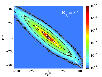
Figure 1: The joint probability density function (PDF) between $p_{C}/\varepsilon$ (horizontal) and $p_{L}/\varepsilon$ (vertical) at $R_{\lambda}=275$, color-coded in a logarithmic scale (see color-bar). Equal-probability contours, separated by factors of $10$, are shown. The PDF is concentrated close to the $p_{C}+p_{L}=0$ line, indicating that the two quantities $p_{C}$ and $p_{L}$ are nearly anti-correlated with each other. The black dashed line shows $\langle p_{L}|p_{C}\rangle/\varepsilon$, which is approximately $-0.86\times p_{C}/\varepsilon$. The white dashed line shows $\langle p_{C}|p_{L}\rangle/\varepsilon$, which is approximately $-p_{L}/\varepsilon$.

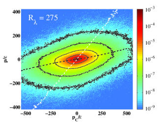
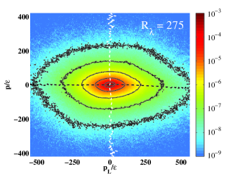
Figure 2: (a) The joint PDF between $p_{C}/\varepsilon$ (horizontal) and $p/\varepsilon$ (vertical), and (b) The joint PDF between $p_{L}/\varepsilon$ (horizontal) and $p/\varepsilon$ (vertical), all at $R_{\lambda}=275$, color-coded in a logarithmic scale (see color-bar). The equal-probability contours shown are separated by factors of $10$. Note that the ranges of values of $p/\varepsilon$ shown are smaller than those of $p_{C}/\varepsilon$ and $p_{L}/\varepsilon$. In (a), the black dashed line represents the conditional average of $p/\varepsilon$ on $p_{C}/\varepsilon$, and is very close to $\langle p|p_{C}\rangle/\varepsilon\approx 0.14\times p_{C}/\varepsilon$. The white dashed line corresponds to the averaged of $p_{C}/\varepsilon$, conditioned on $p/\varepsilon$, and is well approximated by $\langle p_{C}|p\rangle/\varepsilon\approx p/\varepsilon$. In (b), the black dashed line represents the conditional average of $p/\varepsilon$ on $p_{L}/\varepsilon$, and is very close to $\langle p|p_{L}\rangle/\varepsilon\approx 0$. The white dashed line indicates to the average of $p_{L}/\varepsilon$, conditioned on $p/\varepsilon$, and is also very well approximated by $\langle p_{L}|p\rangle/\varepsilon\approx 0$.

IV.2 Cancellation between $p_{L}$ and $p_{C}$

We note that in homogeneous and stationary flows, the first moments of $p$, $p_{C}$ and $p_{L}$ are all exactly $0$. Table 1 shows that the correlation coefficient between $p_{L}$ and $p_{C}$: $\langle p_{C}p_{L}\rangle/(\langle p_{C}^{2}\rangle\langle p_{L}^{2}\rangle)^{1/2}$, is approximately $-0.9$ and seems to approach $-1$ as the Reynolds number increases. This strong anti-correlation results in significant cancellation between $p_{C}$ and $p_{L}$, so the variance of $p$ is much smaller than those of $p_{C}$ and $p_{L}$.

Although the range of values of $R_{\lambda}$ covered by the present study is not sufficient to reach unambiguous conclusions, our results are generally consistent with the expected scalings: $\langle p_{L}^{2}\rangle\sim\langle p_{C}^{2}\rangle\propto R_{\lambda}^{2}$, and $\langle p^{2}\rangle\propto R_{\lambda}^{4/3}$ Xu et al. (2014).

Further insight into the strong cancellation between $p_{C}$ and $p_{L}$ can be gained by studying the joint probability density function (PDF) of $p_{C}$ and $p_{L}$, shown in Fig. 1 for our flow at $R_{\lambda}=275$. Fig. 1 clearly indicates that with a high probability, the values of $p_{C}$ and $p_{L}$ are concentrated close to the line $p_{C}+p_{L}=0$, thus implying a significant cancellation between the two quantities. The observed tendency of the correlation coefficient between $p_{C}$ and $p_{L}$ to approach $-1$ as the Reynolds number increases implies that the joint PDF of $p_{C}$ and $p_{L}$ becomes increasingly concentrated around the line $p_{L}+p_{C}=0$ at higher Reynolds numbers. In all our numerical simulations, we find an approximately linear relation between the conditional average $\langle p_{L}|p_{C}\rangle$ and $p_{C}$ (shown as the black dashed line in Fig. 1): $\langle p_{L}|p_{C}\rangle\approx-\beta(R_{\lambda})p_{C}$, where the dimensionless coefficient $\beta(R_{\lambda})$ depends weakly on $R_{\lambda}$. In agreement with the observed tendency of $p_{L}$ and $p_{C}$ to become increasingly anti-correlated as $R_{\lambda}$ increases, we find that $\beta(R_{\lambda})$ slightly increases with the Reynolds number, see Table 1. This implies that $\langle p|p_{C}\rangle\approx(1-\beta)p_{C}$, where the coefficient $1-\beta$ decreases as $R_{\lambda}$ increases, from $\approx 0.17$ at $R_{\lambda}=193$ to $\approx 0.10$ at $R_{\lambda}=430$. We also observe that the average of $p_{C}$ conditioned on $p_{L}$, shown as the white dashed line in Fig. 1 is almost exactly equal to $-p_{L}$, which implies that $\langle p|p_{L}\rangle\approx 0$.

Fig. 2 shows the joint PDFs of $p_{C}$ and $p$ (a) and of $p_{L}$ and $p$ (b). The conditional averages $\langle p|p_{C}\rangle$ and $\langle p|p_{L}\rangle$ are shown as black dashed lines, whereas the conditional averages $\langle p_{C}|p\rangle$ and $\langle p_{L}|p\rangle$ are shown as white dashed lines. The conditional averages of $p_{C}$ and $p_{L}$ on $p$ have the particularly simple forms: $\langle p_{C}|p\rangle\approx p$ and $\langle p_{L}|p\rangle\approx 0$. In addition, the joint PDF of $p$ and $p_{L}$ is almost symmetrical to both $p=0$ and $p_{L}=0$. The power $p$ is therefore well correlated with $p_{C}$, but not with $p_{L}$.

IV.3 Prevalence of $p_{C}$ on the moments of $p$

IV.3.1 General assumptions

The prevalence of $p_{C}$ on the statistical properties of $p$ shown by our numerical results leads to the conclusion that the second and third moment of $p$ are expressible in terms of the corresponding moments of $p_{C}$. To justify this claim, we use the two following results.

A The numerical results shown in Fig. 1 demonstrate that at a fixed value of $p_{C}$, $p_{L}|p_{C}$ fluctuates around the mean value $\langle p_{L}|p_{C}\rangle\approx-\beta p_{C}$. This immediately implies the following relations:

$$\langle p_{L}p_{C}\rangle=-\beta\langle p_{C}^{2}\rangle\mbox{ and }\langle p_{L}p_{C}^{2}\rangle=-\beta\langle p_{C}^{3}\rangle,$$ (13)

which can be easily justified by writing $p_{L}$ conditioned on a value of $p_{C}$ as:

$$p_{L}|p_{C}=-\beta p_{C}+\xi|p_{C},$$ (14)

where $\xi|p_{C}$ is a random variable with zero mean and its distribution depends on $p_{C}$. Eq. (13) is found to be numerically extremely well satisfied, see Table 2, as a direct consequence of the quality of the linear dependence between $\langle p_{L}|p_{C}\rangle$ and $p_{C}$.

B The lack of correlation between $p$ on $p_{L}$, demonstrated in Fig. 2 and manifested by the two relations $\langle p_{L}|p\rangle\approx 0$ and $\langle p|p_{L}\rangle\approx 0$, implies that:

$$\langle pp_{L}\rangle\approx\langle p^{2}p_{L}\rangle\approx\langle pp_{L}^{2}\rangle\approx 0.$$ (15)

The equalities shown in Eq. (15) are only approximate. In the following, we explore the consequences of the independence between $p$ and $p_{L}$ by assuming for now that these equalities are exactly satisfied, leaving for later a discussion of the errors made.

As we show below the approximations A and B above lead to a very accurate prediction of all the second moments of $p_{C}$, $p_{L}$ and $p$, in terms of $\langle p_{C}^{2}\rangle$ and $\beta$. The predictions concerning the third moments, however, are not as accurate as those concerning the second moments, as a consequence of quantitative deviations from the symmetry assumption B.

IV.3.2 Second moments

Using Eq. (13), $\langle p_{L}p_{C}\rangle=-\beta\langle p_{C}^{2}\rangle$, and Eq. (15), $\langle pp_{L}\rangle=0$, we determine the second moment of $p_{L}$ as a function of $\langle p_{C}^{2}\rangle$: $\langle p_{L}^{2}\rangle=\beta\langle p_{C}^{2}\rangle$, from which we obtain:

$$\langle p^{2}\rangle=(1-\beta)\langle p_{C}^{2}\rangle.$$ (16)

We find that the condition of independence $\langle pp_{L}\rangle=0$ is very well satisfied, which implies that Eq. (16) is numerically very accurately satisfied (see Appendix B and Table 4).

IV.3.3 Third moments

The results from Eq. (12), showing that $\langle p_{C}^{3}\rangle\approx-\varepsilon^{3}R_{\lambda}^{3}$, together with the observation that $\langle p^{3}\rangle\approx-\varepsilon^{2}R_{\lambda}^{2}$ Xu et al. (2014), also point to a strong cancellation between $p_{C}$ and $p_{L}$ in the third moment $\langle p^{3}\rangle$. To relate the properties of the third moments of $p$ to $\langle p_{C}^{3}\rangle$, we begin by noting that Eq. (15) leads to the following expressions for the third order moments: $\langle p_{L}^{3}\rangle=-\beta\langle p_{C}^{3}\rangle$ and $\langle p_{L}^{2}p_{C}\rangle=\beta\langle p_{C}^{3}\rangle$, and hence to the expression $\langle p^{3}\rangle=(1-\beta)\langle p_{C}^{3}\rangle$. These expressions predict simple relations between the various moments $\langle p_{C}^{m}p_{L}^{n}\rangle$ with $m+n=3$ and $\langle p_{C}^{3}\rangle$, and lead to the correct sign of $\langle p^{3}\rangle$, thus justifying our claim that the assumption of independence beween $p$ and $p_{L}$ imposes that the sign of $\langle p^{3}\rangle$ is given by $\langle p_{C}^{3}\rangle$.

The expressions obtained above, however, are quantitatively not accurate. The reason is that while $\langle p_{L}p^{2}\rangle$ is found to be very small (of the order of $1\%$ of $|\langle p_{C}^{3}\rangle|$), the numerical values of $\langle p_{L}^{2}p\rangle$ are found to be much larger, of the order of $10\%$ of $|\langle p_{C}^{3}\rangle|$. The small, but significant error in $\langle p_{L}^{2}p\rangle=0$ therefore leads to a significant reduction of the numerical value of $\langle p^{3}\rangle$, consistent with the numerical values shown in Table 2. To take the effect of non-zero $\langle p_{L}^{2}p\rangle$ into account, we denote $\zeta=\langle p_{L}^{2}p\rangle/\langle p_{C}^{3}\rangle$, where $\zeta$ is a positive number of order $\sim 0.1$ (see Table 2). and decreases when $R_{\lambda}$ increases. This then leads to $\langle p_{L}^{2}p_{C}\rangle=(\beta-\zeta)\langle p_{C}^{3}\rangle$ and $\langle p_{L}^{3}\rangle=-(\beta-2\zeta)\langle p_{C}^{3}\rangle$, and consequently:

$$\langle p^{3}\rangle=(1-\beta-\zeta)\langle p_{C}^{3}\rangle.$$ (17)

Using Eq. (17) and the relation between $\langle p_{C}^{3}\rangle$ and vortex stretching, Eq. (11), we obtain:

$$\langle p^{3}\rangle=-\frac{2}{35}(1-\beta-\zeta)\langle|\mathbf{u}|^{6}\rangle\langle\mathbf{\omega}\cdot\mathbf{S}\cdot\mathbf{\omega}\rangle,$$ (18)

which establishes a quantitative relation between the time irreversibility, as measured by $\langle p^{3}\rangle$, and vortex stretching, a small-scale generation mechanism in 3D turbulence.

We note that Eq. (16), together with the observed scaling $\langle p^{2}\rangle\propto R_{\lambda}^{4/3}$ and $\langle p_{C}^{2}\rangle\propto R_{\lambda}^{2}$, suggests that $(1-\beta)\propto R_{\lambda}^{-2/3}$. Similarly, the dependence $\langle p_{C}^{3}\rangle\propto R_{\lambda}^{3}$, together with the observation of Xu et al. (2014) that $\langle p^{3}\rangle\approx-\varepsilon^{3}R_{\lambda}^{2}$, imply, using Eq. (17), that $(1-\beta-\zeta)\propto R_{\lambda}^{-1}$ or $1-\zeta/(1-\beta)\propto R_{\lambda}^{-1/3}$. These are consistent with the values obtained numerically. As shown in Table 2, the value of $1-\zeta/(1-\beta)$ decreases slightly, from $0.36$ to $0.34$, when the Reynolds number increases from $R_{\lambda}=193$ to $430$.

The results presented here thus show that, while the statement of independence between $p$ and $p_{L}$ is merely an enticing approximation, taking quantitatively into account the deviations from Eq. (15) does not affect our main conclusion: the third moment of $p$ is controlled by the third moment of $p_{C}$.

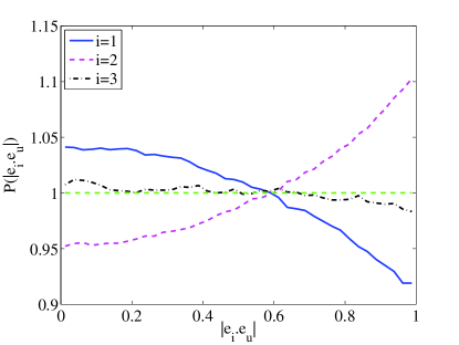
Figure 3: The PDFs of the cosines of the angles between the direction of the velocity $\mathbf{u}$, and the eigenvectors $\mathbf{e}_{i}$ of $\mathbf{S}$ at $R_{\lambda}=275$. The cosine of the angles is given by the inner product of the two unit vectors: $\hat{x}_{i}=\mathbf{e}_{i}\cdot\mathbf{e}_{u}$, where $\mathbf{e}_{u}=\mathbf{u}/|\mathbf{u}|$. A lack of correlation between $\mathbf{u}$ and $\mathbf{S}$ would lead to a flat PDF of $\mathbf{e}_{i}\cdot\mathbf{e}_{u}$: ${\cal P}(|\mathbf{e}_{i}\cdot\mathbf{e}_{u}|)=1$, which are supported by the data to a good degree. The small departure from this expectation points to a weak correlation between $\mathbf{u}$ and $\mathbf{S}$.

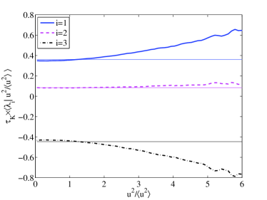
Figure 4: The thick lines show the conditional averages of the eigenvalues of $\mathbf{S}$, $\langle\lambda_{i}|\mathbf{u}^{2}\rangle$, made dimensionless by $\tau_{K}=1/(2\langle\mathbf{S}^{2}\rangle)^{1/2}=1/(2\sum\lambda_{i}^{2})$. The thin lines with the same color are the corresponding unconditional averages $\langle\lambda_{i}\rangle$, all at $R_{\lambda}=275$. For small values of $\mathbf{u}^{2}$, the conditional averages are nearly the same as the corresponding unconditional averages, consistent with the assumption that $\mathbf{u}$ and $\mathbf{S}$ are uncorrelated. For large $\mathbf{u}^{2}$, the magnitudes of the conditional averages increase with $\mathbf{u}^{2}$, indicating a deviation from the assumption. Note that because the probability of having large values of $\mathbf{u}^{2}$ decreases very rapidly with $\mathbf{u}^{2}$, the increases of $\langle\lambda_{i}|\mathbf{u}^{2}\rangle$ at large $\mathbf{u}^{2}$ have only very small effects on the unconditional averages $\lambda_{i}$.

IV.4 Lack of correlation between $\mathbf{u}$ and $\mathbf{S}$

We return here briefly to discuss the essential assumption that $\mathbf{u}$ and $\mathbf{S}$ are uncorrelated. Specifically, we examine in this subsection the correlation between the angles of $\mathbf{u}$ and the eigenvectors $\mathbf{e}_{i}$ and between the magnitude of $\mathbf{u}$ and the eigenvalues $\lambda_{i}$. In the following, the values $\lambda_{i}$ are sorted in decreasing order: $\lambda_{1}\geq\lambda_{2}\geq\lambda_{3}$.

Fig. 3 shows the PDFs of $|\hat{x}_{i}|=|\mathbf{e}_{i}\cdot\mathbf{e}_{u}|$, the absolute value of the cosine of the angle between the eigenvector $\mathbf{e}_{i}$ and the unit vector in the direction of the velocity $\mathbf{e}_{u}=\mathbf{u}/|\mathbf{u}|$ (the sign of this cosine is immaterial) at $R_{\lambda}=275$. A complete lack of correlation between $\mathbf{u}$ and $\mathbf{S}$ implies that the PDFs of $|\mathbf{e}_{i}\cdot\mathbf{e}_{u}|$ are constant and equal to $1$. Fig. 3 shows that this is close to be true. Namely, the probability of alignment between $\mathbf{e}_{1}$ and $\mathbf{u}$, i.e., of $|\mathbf{e}_{u}\cdot\mathbf{e}_{1}|$ being close to $1$, is slightly reduced. On the contrary, the probability of alignment between $\mathbf{e}_{u}$ and $\mathbf{e}_{2}$ is slightly increased. The deviations observed numerically are weak, less than $\sim 10\%$, compared to the uniform distribution. The cosine between $\mathbf{e}_{u}$ and $\mathbf{e}_{3}$, is very close to being uniformly distributed. The nearly uniform PDF of $|\mathbf{e}_{i}\cdot\mathbf{e}_{u}|$ indicate that the assumption that $\mathbf{S}$ and $\mathbf{u}$ are uncorrelated, explicitly used in the determination of $\langle p_{C}^{3}\rangle$, provides a very good first order approximation.

The assumption that $\mathbf{u}$ and $\mathbf{S}$ are uncorrelated also implies that the conditional averages of the properties of $\mathbf{S}$ should be independent of the magnitude of $\mathbf{u}$.

Fig. 4 shows that the dependence of the conditional average of the eigenvalues of $\mathbf{S}$ on $\mathbf{u}^{2}$, $\langle\lambda_{i}|\mathbf{u}^{2}\rangle$, is weak. Systematic deviations are visible at large values of $\mathbf{u}^{2}$, where the magnitudes of the averaged conditional eigenvalues are larger. The probability of large values of $\mathbf{u}^{2}$, however, drops very rapidly when $\mathbf{u}^{2}$ increases Falkovich and Lebedev (1997); Gotoh et al. (2002); Wilczek et al. (2011), so the effect of this weak dependence of $\lambda_{i}$ on $\mathbf{u}^{2}$ has only a small effect on the low-order moments of $p_{C}$ studied here.

In summary, the results presented here and in the Appendix C show that the assumption of a lack of correlation between $\mathbf{u}$ and $\mathbf{S}$ provides a very good first-order approximation to describe the third moment of $p_{C}$.

V Discussion and Conclusion

Our work, aimed at understanding the third moment of the power $p$ acting on fluid particles $\langle p^{3}\rangle\approx-\varepsilon^{3}R_{\lambda}^{2}$, and its implication for the physics of turbulent flows Xu et al. (2014), rests on decomposing $p$ into two parts: a local part, $p_{L}=\mathbf{u}\cdot\partial_{t}\mathbf{u}$, induced by the change of the kinetic energy at a fixed spatial point, and a convective part, $p_{C}=\mathbf{u}\cdot\nabla(\mathbf{u}^{2}/2)$, due to the change in kinetic energy along particle trajectories, assuming the velocity field is frozen. We observe that the two terms $p_{C}$ and $p_{L}$ cancel each other to a large extent, resulting in a much smaller variance of $p$ compared to those of either $p_{C}$ or $p_{L}$. This cancellation may be qualitatively explained by invoking a fast sweeping of the small scales of the flow by the large scales Tennekes (1971). In physical words, kinetic energy along particle trajectories, is mostly carried (swept) by the flow, and changes far less than it would change by keeping the flow fixed, or by varying the flow with the same position in time. This fact has been documented in a slightly different context Kamps et al. (2009). Our results provide a quantitative characterization of how much sweeping reduce the individual contributions of $p_{L}$ and $p_{C}$.

One of the two main results of our work is that the third moment of $p_{C}$, expressed in terms of the rate of strain, $\mathbf{S}$, and the velocity, $\mathbf{u}$, as: $p_{C}=\mathbf{u}\cdot\mathbf{S}\cdot\mathbf{u}$, can be exactly determined, by using the physically justified approximation that $\mathbf{u}$ and $\mathbf{S}$ are uncorrelated. Remarkably, we find that $\langle p_{C}^{3}\rangle$ is directly related to vortex stretching, $\langle\mathbf{\omega}\cdot\mathbf{S}\cdot\mathbf{\omega}\rangle$. In particular, the negative sign of $\langle p_{C}^{3}\rangle$ originates from the positive sign of the vortex stretching, due to small-scale generation by turbulence. This observation provides the first basis for our claim that the third moment of $p$ is related to the generation of small scales in 3D turbulent flows.

The other main observation of our work is that, despite the strong cancellation between $p_{L}$ and $p_{C}$, the power $p$ correlates with $p_{C}$, but not with $p_{L}$, as revealed by the nearly vanishing conditional averages $\langle p|p_{L}\rangle\approx 0$ and $\langle p_{L}|p\rangle\approx 0$. Assuming these conditional averages are exactly zero leads to a simple relation between $\langle p^{3}\rangle$ and $\langle p_{C}^{3}\rangle$. The (weak) corrections to this simple assumption modify only quantitatively the results.

Taken together, these two observations, namely that $\langle p^{3}\rangle$ is controlled by $\langle p_{C}^{3}\rangle$ and that $\langle p_{C}^{3}\rangle$ is directly linked to vortex stretching, $\langle\mathbf{\omega}\cdot\mathbf{S}\cdot\mathbf{\omega}\rangle>0$, allow us to establish a relation between the third moment of power, $\langle p^{3}\rangle$, and vortex stretching. Thus, the recently observed manifestation of irreversibility in studying the statistics of individual Lagrangian trajectories can be understood as resulting from small-scale generation in 3D turbulent flow.

For lack of essential information concerning the quantities investigated here, our work rests on several assumptions supported by numerical observations. The well-known fact that velocity, $\mathbf{u}$, and the rate of strain, $\mathbf{S}$, are dominated by large- and small-scales, respectively, makes it plausible that these two quantities are mostly uncorrelated. Our numerical results confirm this expectation. Although small, and of little relevance for the low-order moments studied here, the deviations observed suggest an interesting structure, which would be worth elucidating. The observation that $p$ and $p_{L}$ are not correlated, in the sense that the conditional averages $\langle p|p_{L}\rangle$ and $\langle p_{L}|p\rangle$ are both very close to zero, rests only on numerical observations, and requires a proper explanation. Understanding and quantifying the weakness of the correlation between $p$ and $p_{L}$ in 3D turbulent flows may provide important hints not only on higher moments of $p$, but more importantly, on the structure of the flow itself.

We note that studying the cancellation between $p_{C}$ and $p_{L}$ by directly focusing on the effect of the pressure gradient, $-\mathbf{u}\cdot\nabla P$ is likely to lead to satisfactory results when studying the second moments of $p$, as the pressure term has been documented to provide the largest contribution to the variance $\langle p^{2}\rangle$ Pumir et al. (2014). In 3D, however, the third moment $-\langle(\mathbf{u}\cdot\nabla P)^{3}\rangle$ has been shown to contribute negligibly to $\langle p^{3}\rangle$, whose understanding requires the investigation of other correlations Pumir et al. (2014).

Finally, the arguments provided here to explain the negative third moments of power fluctuations of particles in 3D turbulent flows should not be applied to 2D turbulence, in which the third moment of $p$ is also negative, and grows with a similar power of the Reynolds number Xu et al. (2014), but the amplification of large velocity gradients is due to entirely different physical processes Boffetta and Ecke (2012). Still, one may expect that the manifestations of irreversibility, in 2D turbulence as well as in a broad class of non-equilibrium systems, to be fundamentally related to a flux in the system.

Appendix A: Alternative expressions of the third moment of $p_{C}$

$R_{\lambda}$	$193$	$275$	$430$
$225\langle p_{C}^{3}\rangle/(7\varepsilon^{3}R_{\lambda}^{3})$	$-0.24$	$-0.37$	$-0.40$
$\frac{\sqrt{15}}{7}\times S_{p_{C}}$	$-0.30$	$-0.38$	$-0.42$
$S_{p}\equiv\langle p^{3}\rangle/\langle p^{2}\rangle^{3/2}$	$-0.52$	$-0.62$	$-0.67$

Table 3: Third moments of the distributions of $p_{C}/\varepsilon$ and $p/\varepsilon$ at the three Reynolds numbers studied in this article.

In many experiments and numerical simulations, the probability distributions of individual components of velocity $\mathbf{u}$ are close to Gaussian Wilczek et al. (2011). That observation allows us to estimate explicitly the $6^{th}$ moment of $|\mathbf{u}|$ in terms of the second moment:

$$\langle|\mathbf{u}|^{4}\rangle=\frac{5}{3}\langle|\mathbf{u}|^{2}\rangle^{2}~{},~{}~{}\langle|\mathbf{u}|^{6}\rangle=\frac{35}{9}\langle|\mathbf{u}|^{2}\rangle^{3},$$ (19)

which, when substituted into Eq. (11), gives an expression for $\langle p_{C}^{3}\rangle$ as:

$$\langle p_{C}^{3}\rangle=\frac{8}{27}\langle|\mathbf{u}|^{2}\rangle^{3}\langle\textrm{tr}(\mathbf{S}^{3})\rangle.$$ (20)

The same assumptions and similar elementary algebraic manipulations as those used to establish Eq. (20), lead to an exact expression for the second moment of $p_{C}$:

$$\langle p_{C}^{2}\rangle=\frac{2}{15}\langle|\mathbf{u}|^{4}\rangle\langle\textrm{tr}(\mathbf{S}^{2})\rangle=\frac{1}{15}R_{\lambda}^{2}\varepsilon^{2},$$ (21)

This relation is found to be in very good agreement with our numerical results, see Table 1.

The known relation between $\textrm{tr}(\mathbf{S}^{3})$ and the experimentally accessible moments of $\partial_{x}u_{x}$ Betchov (1956):

$$\langle\textrm{tr}(\mathbf{S}^{3})\rangle=\frac{105}{8}\langle(\partial_{x}u_{x})^{3}\rangle,$$ (22)

together with the expression for the second moment of $\partial_{x}u_{x}$: $\langle(\partial_{x}u_{x})^{2}\rangle=\varepsilon/(15\nu)$ Tennekes and Lumley (1972); Frisch (1995), leads to the following expression for the third moment of $p_{C}$:

$$\langle p_{C}^{3}\rangle=\frac{7}{225}S_{\partial_{x}u_{x}}R_{\lambda}^{3}\varepsilon^{3},$$ (23)

where $S_{\partial_{x}u_{x}}\equiv\langle(\partial_{x}u_{x})^{3}\rangle/\langle(\partial_{x}u_{x})^{2}\rangle^{3/2}$ is the skewness of the velocity derivative.

Combining Eq. (21) and (23) gives the following relation between the skewness of $\partial_{x}u_{x}$ and the skewness of $p_{C}$:

$$S_{\partial_{x}u_{x}}=\frac{\sqrt{15}}{7}S_{p_{C}}.$$ (24)

The values of $\frac{\sqrt{15}}{7}S_{p_{C}}$, as well as the ratio $225\langle p_{C}^{3}\rangle/(7\varepsilon^{3}R_{\lambda}^{3})$, determined from our numerical simulations, are shown in Table 3. The correponding value of the skewness of $\partial_{x}u_{x}$, $S_{\partial_{x}u_{x}}$ is found to be approximately $\approx-0.4$, which is well within the range of values of $S_{\partial_{x}u_{x}}$ reported from experiments and simulations at comparable Reynolds numbers Sreenivasan and Antonia (1997); Ishihara et al. (2007).

Appendix B: Prevalence of $p_{C}$ on the moments of $p$

$R_{\lambda}$	$193$	$275$	$430$
$\langle p_{L}~{}p_{C}\rangle/\langle p_{L}^{2}\rangle^{1/2}\langle p_{C}^{2}\rangle^{1/2}$	$-0.907$	$-0.923$	$-0.944$
$-\beta^{1/2}$	$-0.912$	$-0.928$	$-0.947$
$\langle p^{2}\rangle/\langle p_{C}^{2}\rangle$	$0.178$	$0.147$	$0.110$
$1-\beta$	$0.17$	$0.14$	$0.10$
$\langle p_{L}^{2}\rangle/\langle p_{C}^{2}\rangle$	$0.823$	$0.851$	$0.892$
$\beta$	$0.83$	$0.86$	$0.90$

Table 4: Parametrisation of the second moments of $p_{C}/\varepsilon$, $p_{L}/\varepsilon$ and $p/\varepsilon$, compared to the expression in terms of $\beta$ given by Eq. 25,26 and 27, at the three Reynolds numbers studied in this article.

V.1 Second moments of $p$

The decomposition of the distribution of $p_{L}$ conditioned on $p_{C}$, see Eq. (14), involving a random variable $\xi|p_{C}$ with a zero mean, together with the assumption of independence between $p$ and $p_{L}$, $\langle pp_{L}\rangle=0$ (see Eq. (15)), leads to a full description of the second moments of $p_{C}$, $p_{L}$ in terms of $\beta$ only:

$$\langle p_{L}^{2}\rangle =\beta\langle p_{C}^{2}\rangle$$ (25)

$$\langle p_{L}p_{C}\rangle =-\beta\langle p_{C}^{2}\rangle=-\beta^{1/2}(\langle p_{C}^{2}\rangle\langle p_{L}^{2}\rangle)^{1/2}$$ (26)

$$\langle p^{2}\rangle =(1-\beta)\langle p_{C}^{2}\rangle$$ (27)

The values of $\beta$ are measured from the conditional average $\langle p_{L}|p_{C}\rangle=-\beta p_{C}$, Eq. (14). This allows us to check how accurately are Eqs. (25) to (27) satisfied. The numerical results are shown in Table 4. The relations given by Eqs. (25) to (27) are found to be very well satisfied, with very small errors, thus demonstrating that the proposed parametrization in terms of $\langle p_{C}^{2}\rangle$ and $\beta$ provides a very good description of the second moments of $p$.

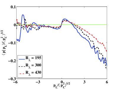
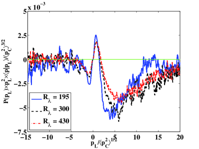
Figure 5: The conditional average of $p$ on $p_{L}$: (a) raw data $\langle p|p_{L}\rangle/\langle p_{C}^{2}\rangle^{1/2}$ vs. $p_{L}/\langle p_{C}^{2}\rangle^{1/2}$ and (b) $\mathcal{P}(p_{L})\langle p|p_{L}\rangle p_{L}^{2}/\langle p_{C}^{2}\rangle^{3/2}$, which provides the integrand in Eq. (28) to calculate the normalized third moment $\langle p_{L}^{2}p\rangle/\langle p_{C}^{2}\rangle^{3/2}=\zeta S_{p_{C}}$. The conditional average $\langle p|p_{L}\rangle$ differs weakly, but consistently from being $0$, especially for $p_{L}>0$, where the conditional average $\langle p|p_{L}\rangle$ decreases approximately linearly. This leads to an appreciable negative contribution to $\langle p_{L}^{2}p\rangle$: $\zeta=\langle p_{L}^{2}p\rangle/\langle p_{C}^{3}\rangle\lesssim 10$% in the range of Reynolds number studied.

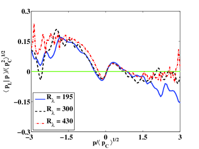
Figure 6: The conditional PDF of $p_{L}$ on $p$: (a) $\langle p_{L}|p\rangle/\langle p_{C}^{2}\rangle^{1/2}$ vs. $p/\langle p_{C}^{2}\rangle^{1/2}$, and (b) $\mathcal{P}(p)\langle p_{L}|p\rangle p^{2}/\langle p_{C}^{2}\rangle^{3/2}$. The areas under the curves in panel (b) give the normalized third moment $\langle p^{2}p_{L}\rangle/\langle p_{C}^{2}\rangle^{3/2}$, which are much smaller than those for $\langle p_{L}^{2}p\rangle/\langle p_{C}^{2}\rangle^{3/2}$ in Fig. 5(b).

V.2 Conditional averages $\langle p|p_{C}\rangle$ and $\langle p_{C}|p\rangle$

Crucial to the argument relating the third moment $\langle p^{3}\rangle$ to the third moment of $p_{C}$ is the observation that the conditional averages $\langle p|p_{L}\rangle$ and $\langle p_{L}|p\rangle$ are close to $0$. Figure 2b of the main text shows these averages $(p_{L},\langle p|p_{L}\rangle)$ and $(\langle p_{L}|p\rangle,p)$, which appear as horizontal and vertical straight lines respectively on the scale of the figure. Our argument is then based on identities such as:

$$\langle p_{L}^{2}p\rangle=\int_{-\infty}^{\infty}\mathcal{P}(p_{L})\langle p|p_{L}\rangle p_{L}^{2}dp_{L},$$ (28)

where $\mathcal{P}(p_{L})$ is the PDF of $p_{L}$. Equation (28) shows that if $\langle p_{L}|p\rangle=\langle p|p_{L}\rangle=0$, then, $\langle p^{2}p_{L}\rangle=\langle p_{L}^{2}p\rangle=0$.

Possible deviations from zero of the moments $\langle p_{L}^{2}p\rangle$ and $\langle p^{2}p_{L}\rangle$ therefore indicate that the conditional averages $\langle p|p_{L}\rangle$ and $\langle p_{L}|p\rangle$ are not exactly zero. These moments can be readily estimated from the various third moments $\langle p_{C}^{m}p_{L}^{n}\rangle$ with $m+n=3$ shown in Table 2 of the main text:

$$\langle p^{2}p_{L}\rangle=\langle p_{C}^{2}p_{L}\rangle+2\langle p_{C}p_{L}^{2}\rangle+\langle p_{L}^{3}\rangle$$ (29)

and

$$\langle p_{L}^{2}p\rangle=\langle p_{L}^{3}\rangle+\langle p_{L}^{2}p_{C}\rangle.$$ (30)

When compared to $\langle p_{C}^{3}\rangle$, the value of $\langle p^{2}p_{L}\rangle$ is approximately zero ( $|\langle p^{2}p_{L}\rangle/\langle p_{C}^{3}\rangle|\lesssim 2$%), but $\langle p_{L}^{2}p\rangle/\langle p_{C}^{3}\rangle\lesssim 10$%. This points to a departure of $\langle p|p_{L}\rangle$ from being $0$, which we explore here.

Figure 5 shows the conditional averages of $\langle p|p_{L}\rangle$ for the three direct numerical simulation (DNS) runs discussed in this article, and also the integrand in Eq. (28). For all three cases, the curves differ weakly but consistently from $0$. While for $p_{L}<0$, the values of $\langle p|p_{L}\rangle$ are very small, they differ noticeably from $0$ on the positive $p_{L}$ side, with an approximately linear dependence on $p_{L}$. In order to examine the effect of this deviation of $\langle p|p_{L}\rangle$ on $\zeta=\langle p_{L}^{2}p\rangle/\langle p_{C}^{3}\rangle$, we non-dimensionalize the variables $p_{L}$ and $p$ in Fig. 5 by $\langle p_{C}^{2}\rangle^{1/2}$. In particular, in Fig. 5(b), we plot $\mathcal{P}(p_{L})\langle p|p_{L}\rangle p_{L}^{2}/\langle p_{C}^{2}\rangle^{3/2}$. In this way, the areas under the curves in Fig. 5(b) give $\langle p_{L}^{2}p\rangle/\langle p_{C}^{2}\rangle^{3/2}=\zeta S_{p_{C}}$, where $S_{p_{C}}=\langle p_{C}^{3}\rangle/\langle p_{C}^{2}\rangle^{3/2}$ is the skewness of $p_{C}$, which depends weakly on the Reynolds number as shown in Table 2 of the main text. Fig. 5(b) shows that $\langle p_{L}^{2}p\rangle/\langle p_{C}^{2}\rangle^{3/2}$ decreases when the Reynolds number increases. This is consistent with the observed decrease of the value of $\zeta$ with the Reynolds number.

As shown in Table 2 of the main text, $\zeta=0.11$, $0.088$ and $0.066$ at $R_{\lambda}=193$, $275$, and $430$, respectively. In fact, over the limited range of Reynolds number that we studied here, we observed that $\zeta/(1-\beta)$ remains well below unity: $\zeta/(1-\beta)\approx 0.64$, which ensures that the third moment of $p$, as given by Eq. [12] in the main text, is determined by $\langle p_{C}^{3}\rangle$:

$$\langle p^{3}\rangle=(1-\beta-\zeta)\langle p_{C}^{3}\rangle=(1-\beta)\left(1-\frac{\zeta}{1-\beta}\right)\langle p_{C}^{3}\rangle.$$ (31)

We note that the scaling of $\langle p^{3}\rangle\sim R_{\lambda}^{2}$ reported before Xu et al. (2014), together with the scalings $\langle p_{C}^{3}\rangle\sim R_{\lambda}^{3}$ and $(1-\beta)\sim R_{\lambda}^{-2/3}$ obtained in this work, implies that $1-[\zeta/(1-\beta)]\sim R_{\lambda}^{-1/3}$. These predictions can only be checked by using DNS at much higher Reynolds numbers, and with adequate statistical resolution.

For comparison, Fig. 6 shows the conditional average of $p_{L}$ on $p$: $\langle p_{L}|p\rangle$ and the integrand of $\langle p^{2}p_{L}\rangle$. As it was the case in Fig. 5, the two quantities $p$ and $p_{L}$ are normalized by $\langle p_{C}^{2}\rangle^{1/2}$ in the way such that the areas under the curves in Fig. 6(b) represent the normalized moment $\langle p^{2}p_{L}\rangle/\langle p_{C}^{2}\rangle^{3/2}=(\langle p^{2}p_{L}\rangle/\langle p_{C}^{3}\rangle)S_{p_{C}}$. A systematic deviation of $\langle p_{L}|p\rangle$ from being $0$ is visible in Fig. 6(a). On the other hand, the integrand $\mathcal{P}(p)p^{2}\langle p_{L}|p\rangle$ is noticeably non-zero only in a small range of $p$, which results in a much smaller value of $\langle p^{2}p_{L}\rangle$ compared to $\langle p_{L}^{2}p\rangle$.

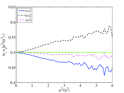
Figure 7: Dependence of the alignment between $\mathbf{e}_{i}$ and $\mathbf{e}_{u}$ on $\mathbf{u}^{2}$ at $R_{\lambda}=275$. Panels (a) (respectively (b) and (c)) show $\mathcal{P}(\mathbf{u}^{2},|\mathbf{e}_{u}\cdot\mathbf{e}_{i}|)$, the joint PDF of $\mathbf{u}^{2}$ and $|\mathbf{e}_{u}\cdot\mathbf{e}_{i}|$ for $i=1$ (respectively $i=2$ and $i=3$). The indicated colour coding refers to the decimal logarithm of the PDF, i.e., $\log_{10}\mathcal{P}(\mathbf{u}^{2},|\mathbf{e}_{u}\cdot\mathbf{e}_{i}|)$. The equal-probability contours, shown as dashed lines, are close to, but deviate from being vertical, which indicates a systematic dependence on $\mathbf{u}^{2}$, especially for $i=1$ and $i=2$. Panel (d) shows the conditional average $\langle|\mathbf{e}_{i}\cdot\mathbf{e}_{u}||\mathbf{u}^{2}\rangle$ vs. $\mathbf{u}^{2}$ (also shown as dash-dotted lines in Panels a-c), which weakly deviates from being constant as implied by the assumption of lack of correlation between $\mathbf{S}$ and $\mathbf{u}$.

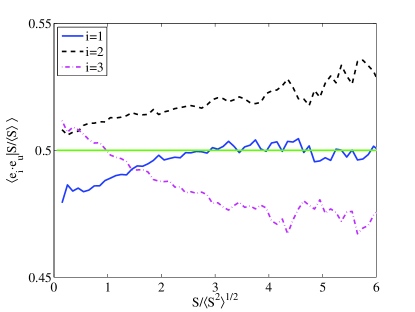
Figure 8: Dependence of the alignment between $\mathbf{e}_{i}$ and $\mathbf{e}_{u}$ on $|\mathbf{S}|$ for $i=1$ (full line), $i=2$ (dashed line) and $i=3$ (dash-dotted line) at $R_{\lambda}=275$. The variation of the conditional average of $|\mathbf{e}_{i}\cdot\mathbf{e}_{u}|$ on $|\mathbf{S}|$ is much weaker than the dependence on $\mathbf{u}^{2}$ shown in Fig. 7.

Appendix C: Lack of correlation between $\mathbf{u}$ and $\mathbf{S}$

The results presented in the main text give a good indication that assuming $\mathbf{u}$ and $\mathbf{S}$ are uncorrelated provides an appropriate first-order approximation. This is in fact corroborated by the quantitative agreement between the numerical results and the predictions. Here we present further information concerning the correlations between $\mathbf{u}$ and $\mathbf{S}$.

The first hint of a correlation between the velocity and strain was provided by Fig. 3 of the main text, which showed weak, but noticeable deviations from a uniform distribution for PDFs of the cosines of the angles between the direction of velocity, $\mathbf{e}_{u}$, and the eigenvectors of strain, especially between $\mathbf{e}_{u}$ and $\mathbf{e}_{1}$ and between $\mathbf{e}_{u}$ and $\mathbf{e}_{2}$.

It may be expected that the alignment between $\mathbf{u}$ and the eigenvectors of $\mathbf{S}$ depends on the magnitude of $\mathbf{u}$. Figure 7 shows the joint probability distribution function between $\mathbf{u}^{2}$ and $|\mathbf{e}_{u}\cdot\mathbf{e}_{i}|$ for $i=1$ (a), $i=2$ (b) and $i=3$ (c). The bending of the equal-probability contours, shown as dashed lines in Fig. 7(a-c) reveals a weak, but systematic dependence of the alignment between $\mathbf{u}$ and $\mathbf{e}_{i}$ as a function of $\mathbf{u}^{2}$. Fig. 7(c) shows that the effect is considerably weaker for $i=3$ than it is for $i=1$ and $i=2$. We observe that the average of $|\mathbf{e}_{i}\cdot\mathbf{e}_{u}|$ conditioned on $\mathbf{u}^{2}$, plotted as the dash-dotted lines in Fig. 7(a-c) and separately in Fig. 7(d), shows clear variations as a function of $\mathbf{u}^{2}$, especially for $i=1$ and $i=2$. The information presented in Fig. 7 thus reveals that $\mathbf{u}^{2}$ influences not only the eigenvalues of strain, as shown in Figure 4 of the main text, but also the statistical properties concerning the orientation of $\mathbf{u}$ with respect to the eigenvectors of $\mathbf{S}$. This in turn induces a dependence of the third and fifth moments of $p_{C}$ on $\mathbf{u}^{2}$ that is more complicated than the expectation based on the lack of correlation between $\mathbf{u}$ and $\mathbf{S}$.

The results shown by Fig. 7 thus show small, but systematic deviations of the statistical quantities relevant to $p_{C}$ from the expected dependence on $\mathbf{u}^{2}$. In comparison, the dependence on the magnitude of $\mathbf{S}$ seems to be much weaker. Figure 8 shows that the value of the average of the cosines of the angles, $|\mathbf{e}_{u}\cdot\mathbf{e}_{i}|$, conditioned on $|\mathbf{S}|$, depends significantly less on $|\mathbf{S}|$: the variations shown in Fig. 8 are of the order of $\sim 5\%$, whereas the ones shown in Fig. 7d are of the order of $\sim 20\%$. This difference points to a stronger dependence of the alignment properties on the large scale features of the flow, than on the small scales.

The results presented in this section thus demonstrate that, while the results obtained in this work by assuming that $\mathbf{u}$ and $\mathbf{S}$ are uncorrelated do provide a good approximation to the third moment of $p_{C}$, small, but systematic deviations from this assumption are visible. Judging from the present results, the dependence on $|\mathbf{u}|$ seems to be generally more important than the dependence on $|\mathbf{S}|$.

References

- Kolmogorov (1941) A. N. Kolmogorov, “The local structure of turbulence in incompressible viscous fluid for very large reynolds number,” Dokl. Akad. Nauk SSSR 30, 301–305 (1941).
- Falkovich et al. (2001) G. Falkovich, K Gawedzki, and M. Vergassola, “Particles and fields in fluid turbulence,” Rev. Mod. Phys. 73, 913–975 (2001).
- Batchelor and Townsend (1947) G. K. Batchelor and A. A. Townsend, “Decay of vorticity in isotropic turbulence,” Proc. R. Soc. Lond. A 190, 534–550 (1947).
- Townsend (1951) A. A. Townsend, “On the fine-scale structure of turbulence,” Proc. R. Soc. Lond. A 208, 534–542 (1951).
- Sreenivasan and Antonia (1997) K. R. Sreenivasan and R. A. Antonia, “The phenomenology of small-scale turbulence,” Annu. Rev. Fluid Mech. 29, 435–472 (1997).
- Ishihara et al. (2007) T. Ishihara, Y. Kaneda, M. Yokokawa, K. Itakura, and A. Uno, “Small-scale statistics in high-resolution direct numerical simulation of turbulence: Reynolds number dependence of one-point velocity gradient statistics,” J. Fluid Mech. 592, 335–366 (2007).
- Betchov (1956) R. Betchov, “An inequality concerning the production of vorticity in isotropic turbulence,” J. Fluid Mech. 1, 497–504 (1956).
- Yeung and Pope (1989) P. K. Yeung and S. B. Pope, “Lagrangian statistics from direct numerical simulations of isotropic turbulence,” J. Fluid Mech. 207, 531–586 (1989).
- La Porta et al. (2001) A. La Porta, G. A. Voth, A. M. Crawford, J. Alexander, and E. Bodenschatz, “Fluid particle accelerations in fully developed turbulence,” Nature 409, 1017–1019 (2001).
- Mordant et al. (2001) N. Mordant, P. Metz, O. Michel, and J.-F. Pinton, “Measurement of Lagrangian velocity in fully developed turbulence,” Phys. Rev. Lett. 87, 214501 (2001).
- Bourgoin et al. (2006) M. Bourgoin, N. T. Ouellette, H. Xu, J. Berg, and E. Bodenschatz, “The role of pair dispersion in turbulent flow,” Science 311, 835–838 (2006).
- Sawford and Yeung (2011) B. L. Sawford and P. K. Yeung, “Kolmogorov similarity scaling for one-particle Lagrangian statistics,” Phys. Fluids 23, 091704 (2011).
- Falkovich et al. (2012) G. Falkovich, H. Xu, A. Pumir, E. Bodenschatz, L. Biferale, G. Boffetta, A. S. Lanotte, and F. Toschi, “On lagrangian single-particle statistics,” Phys. Fluids 24, 055102 (2012).
- Xu et al. (2014) H. Xu, A. Pumir, G. Falkovich, E. Bodenschatz, M. Shats, H. Xia, N. Francois, and G. Boffetta, “Flight-crash events in turbulence,” Proc. Nat. Acad. Sci. USA 111, 7558–7563 (2014).
- Leveque and Naso (2014) E. Leveque and A. Naso, “Introduction of longitudinal and transverse lagrangian velocity increments in homogeneous and isotropic turbulence,” Europhy. Lett. 108, 379–385 (2014).
- Pumir et al. (2014) A. Pumir, H. Xu, G. Boffetta, G. Falkovich, and E. Bodenschatz, “Redistribution of kinetic energy in turbulent flows,” Phys. Rev. X 4, 041006 (2014).
- Obukhov and Yaglom (1951) A. M. Obukhov and A. M. Yaglom, “The microstructure of turbulent flow,” Prikl. Mat. Mekh. 15, 3–26 (1951), English Trans. as NACA TM 1350, 1953.
- Vedula and Yeung (2001) P. Vedula and P. K. Yeung, “Similarity scaling of acceleration and pressure statistics in simulations of isotropic turbulence,” Phys. Fluids 11, 1208–1220 (2001).
- Tennekes (1971) H. Tennekes, “Eulerian and lagrangian time microscales in isotropic turbulence,” J. Fluid Mech. , 561–567 (1971).
- Tsinober et al. (2001) A. Tsinober, P. Vedula, and P. K. Yeung, “Random taylor hypothesis and the behavior of local and convective accelerations in isotropic turbulence,” Phys. Fluids 13, 1974–1984 (2001).
- Gulitski et al. (2007) G. Gulitski, M. Kholmyansky, W. Kinzelbach, B. Lüthi, A. Tsinober, and S. Yorish, “Velocity and temperature derivatives in high-Reynolds-number turbulent flows in the atmospheric surface layer. part 2. accelerations and related matters,” J. Fluid Mech. 589, 83–102 (2007).
- Lamorgese et al. (2005) A. G. Lamorgese, D. A. Caughey, and S. B. Pope, “Direct numerical simulation of homogeneous turbulence with hyperviscosity,” Phys. Fluids 17, 05106 (2005).
- Orszag (1971) S. A. Orszag, “On the elimination of aliasing in finite-difference schemes by filtering high-wavenumber components,” J. Atmos. Sci. 28, 1074 (1971).
- Li et al. (2008) Y. Li, E. Perelman, M. Yuan, Y. Yang, et al., “A public turbulence database cluster and applications to study lagrangian evolution of velocity increments in turbulence,” J. Turbulence 9, N31 (2008).
- Tennekes and Lumley (1972) H. Tennekes and J. L. Lumley, A First Course in Turbulence (The MIT Press, Cambridge, Massachusetts and London, England, 1972).
- Frisch (1995) U. Frisch, Turbulence: The Legacy of A. N. Kolmogorov (Cambridge University Press, Cambridge, England, 1995).
- Siggia (1981) E. D. Siggia, “Invariants for the one-point vorticity and strain rate correlation functions,” Phys. Fluids 24, 1934–1936 (1981).
- Falkovich and Lebedev (1997) G. Falkovich and V. Lebedev, “Single-point velocity distribution in turbulence,” Phys. Rev. Lett. 79, 4159–4161 (1997).
- Wilczek et al. (2011) M. Wilczek, A. Daitche, and R. Friedrich, “On the velocity distribution in homogeneous isotropic turbulence: correlations and deviations from gaussianity,” J. Fluid Mech. 676, 191–217 (2011).
- Gotoh et al. (2002) T. Gotoh, D. Fukayama, and T. Nakano, “Velocity field statistics in homogeneous steady turbulence obtained using a high-resolution direct numerical simulation,” Phys. Fluids 14, 1065–1081 (2002).
- Kamps et al. (2009) O. Kamps, R. Friedrich, and R. Grauer, “Exact relation between eulerian and lagrangian velocity increment statistics,” Phys. Rev. E 79, 066301 (2009).
- Boffetta and Ecke (2012) G. Boffetta and R. E. Ecke, “Two-dimensional turbulence,” Annu. Rev. Fluid Mech. 44, 427–451 (2012).