Tachyon inflation in the large-$N$ formalism

Abstract

We study tachyon inflation within the large-$N$ formalism, which takes a prescription for the small Hubble flow slow–roll parameter $\epsilon_{1}$ as a function of the large number of $e$-folds $N$. This leads to a classification of models through their behaviour at large $N$. In addition to the perturbative $N$ class, we introduce the polynomial and exponential classes for the $\epsilon_{1}$ parameter. With this formalism we reconstruct a large number of potentials used previously in the literature for Tachyon Inflation. We also obtain new families of potentials form the polynomial class. We characterize the realizations of Tachyon Inflation by computing the usual cosmological observables up to second order in the Hubble flow slow–roll parameters. This allows us to look at observable differences between tachyon and canonical single field inflation. The analysis of observables in light of the Planck 2015 data shows the viability of some of these models, mostly for certain realization of the polynomial and exponential classes.

1 Introduction

From its inception, inflation has been a extremely useful mechanism to address several issues which the old cosmology was unable to explain [1]. The inflationary paradigm has involved a vast effort in model building and the variety of models is huge. The nature of the inlfationary field is not yet determined and in principle the tachyon can be responsible for inflation. The tachyon field was brought up to prominence by A. Sen [2, 3] who studied type II string theory and the tachyon instability signals on D-branes. In the context of the brane wold paradigm the tachyon field as also been a subject of study (see for instance [4]) and references there in. The cosmological relevance of the tachyon was first explored in [5, 6, 7], where the expansion of the universe was studied for various initial conditions (see also [9, 10, 8, 11]). Independently of its possible origin in string theory one can simply take the tachyon field as another inflaton candidate and study its implications without trying in a first approximation to understand its origin and theoretical implications.

In the present article we study tachyon inflation in the so called large-$N$ formalism [12, 13, 14], where relevant quantities are functions of the number of $e$-folds $N$, taken as an evolution variable instead of the usual inflaton field $\phi$, or cosmic time. The large-$N$ formalism has been successfully applied to obtain model–independent predictions for the scalar spectral index [15] as well as for the running [14] in the canonical single-field inflation scenario. Interesting results for the excursion $\Delta\phi$ of the inflaton have obtained in [16] within this formalism.

In practice, the large-$N$ formalism is employed to obtain universal classes of inflationary models from the mathematical relations that hold between two general physical conditions, namely a large number of $e$-folds and the smallness of the slow–roll parameters. In the large-$N$ formalism these two requirements are linked in a single prescription to guarantee a long period of inflation. Concretely, these two conditions are linked through an explicit function of the Hubble flow slow–roll parameter $\epsilon_{1}$. An explicit form of $\epsilon_{1}(N)$ allows one to group families of potentials in a single prescription with common functional forms for the observables. The large-$N$ formalism represents a powerful method of extracting important information about complete classes of inflationary models in a condensed way; as opposed to the usual treatment of individual models starting from an explicit potential.

In this paper we describe the large-$N$ formalism in the context of Tachyon Inflation (Sec. 2). In Sec. 3 we consider three different prescriptions of the $\epsilon_{1}(N)$ function which cover most of the models considered so far in tachyon inflation. We also find new classes of potentials, to our knowledge not previously published. We also address in two important questions regarding this model: First a check for stability of the model keeping control over the propagation speed for perturbations $c_{s}$ and the validity of the fluid description by computing the size of entropy perturbations (App. A). The second important question is the non-Gaussianity of the different realizations of the model, which we evaluate in Sec. 3 following previous works [9]. The large-$N$ formalism also works to directly derive the sets of observables in the tachyon. We contrast the cosmological parameters with the recent observations by the joint PLANCK-KECK-BICEP analysis [17], and the BAO-PLANCK data [18], at second order in the slow–roll parameters (see Sec. 4). We use the derived values to demonstrate the relevance of our work for a specific model derived from string theory (Sec. 4.2). Finally, Section 5 contains a discussion of our results and concluding remarks.

2 Tachyon Inflation and the large-$N$ Formalism

The scenario of inflation driven by a tachyon field is described by the action

$$S=\int d^{4}x\sqrt{-g}\left[\frac{1}{16\pi}R-V(T)\left(1+g^{\mu\nu}\partial_{\mu}T\partial_{\nu}T\right)^{1/2}\right]\,.$$ (2.1)

Our background spacetime is the usual homogeneous and isotropic Friedmann-Lemaitre-Robertson-Walker (FLRW) with a metric given by $ds^{2}=-dt^{2}+a(t)^{2}d\bf x^{2}$. Thus, in what follows a prime denotes a derivative with respect to the scalar field and a dot represents a derivative with respect to cosmic time. The relevant equations for this scenario are the Klein-Gordon that encodes the dynamics of the field and the Friedmann equation, given in the background by

$$\ddot{T}+3H\dot{T}(1-\dot{T}^{2})+({\ln V})^{\prime}(1-\dot{T}^{2})=0\,,$$ (2.2)

$$H^{2}=\frac{8\pi}{3}\frac{V}{(1-\dot{T}^{2})^{1/2}}\,,$$ (2.3)

where the units employed are such that $M_{\rm Pl}=(8\pi)^{-1/2}$. The Hubble parameter introduced here is defined as $H=d\ln[a]/dt$. It is natural to introduce the definition of the number of $e$-foldings as a parametrization of the amount of expansion in the inflationary period:

$$N=\int_{t}^{t_{\rm eoi}}H(\tilde{t})\,d\tilde{t}\,,$$ (2.4)

where the subindex _eoi denotes the end of inflation.

The accelerated expansion is usually characterized by a set of slow–roll parameters which directly control the steepness of the inflationary potential. For our purposes we find convenient to introduce the alternative Hubble flow slow–roll parameters, as introduced in Ref. [19]:

$$\epsilon_{0} \equiv H_{*}/H,$$ (2.5)

$$\epsilon_{i+1} \equiv \frac{d\ln|\epsilon_{i}|}{dN},\ \ \ i\geq 0.$$ (2.6)

Here $H_{*}$ is the Hubble parameter at some chosen time, and $\dot{\epsilon}_{i}=H\epsilon_{i}\epsilon_{i+1}$. Inflation is guaranteed if $\epsilon_{1}<1$. The Hubble flow functions $\epsilon_{i}$ are defined in terms of derivatives of $H$ with respect to the number of $e$-folds $N$, and in particular we can write

$$N(T)=\sqrt{\frac{3}{2}}\int_{T}^{{T}_{\rm eoi}}\frac{H}{\sqrt{\epsilon_{1}}}d\tilde{T}\,.$$ (2.7)

This integral is useful in the application of the large-$N$ formalism. To first order in slow–roll, these parameters can be related to derivatives of the potential as it is shown in [8], thus a relation between the usual slow roll parameters and the Hubble flow slow–roll parameter is easily obtained if we consider that, within a slow–roll regime, $3H^{2}\approx V(\phi)$, see reference [20] for a detailed explanation.

In order to solve the system of the Klein-Gordon equation (2.2) plus the Friedmann equation (2.3), one must provide an explicit form of the potential $V(T)$. An alternative set of evolution equations to the Fiedmann/Klein-Gordon set is the following Hamilton-Jacobi system

$$H^{\prime 2} = \frac{9}{4}H^{4}T-16\pi^{2}V^{2},$$ (2.8)

$$H^{\prime} = -\frac{3}{2}H^{2}\dot{T}.$$ (2.9)

This and Eq. (2.6) imply that a form for the first slow–roll parameter is $\epsilon_{1}(N)=\frac{3}{2}\dot{T}^{2}$.

It is thus clear that in this formulation one can specify a function $\epsilon_{1}(N)$ to fully determine the inflationary observables.

The cosmological observables can be written in terms of the $\epsilon_{1}(N)$ parameter as shown in the equations below

$$H(N) = H_{0}\exp\left[\int^{0}_{N}\epsilon_{1}(N)dN\right]\,,$$ (2.10)

$$\epsilon_{2} = -\frac{1}{\epsilon_{1}}\frac{d\epsilon_{1}}{dN}\,,$$ (2.11)

$$\epsilon_{3}\epsilon_{2} = \frac{1}{\epsilon_{1}}\frac{d^{2}\epsilon_{1}}{dN^{2}}-\left(\frac{1}{\epsilon_{1}}\frac{d\epsilon_{1}}{dN}\right)^{2}\,.$$ (2.12)

This last equation shows that the explicit function $\epsilon_{1}(N)$ and the integration of the Hubble parameter in Eq. (2.10) completely determine the evolution of the tachyon field.

A reparametrization of observables may seem unnecessary at first sight. However, there are two main advantages of determining the evolution of fields via $\epsilon_{1}(N)$: Firstly, a more general description of the dynamics is obtained without appealing to a particular form of the potential. This leads to classes of the tachyon model grouped in a single description. A second feature is the more accurate description achieved by employing the Hubble flow slow–roll parameters in terms of $\epsilon_{1}(N)$. This is achieved because, as opposed to the standard slow–roll treatment, in the present formalism the scalar kinetic term is encoded within the Hubble flow parameters.

To completely define the inflationary models at hand, it is desirable to specify the explicit form of the potential $V(T)$. The reconstruction for the dependence $V(N)$ is made after imposing the slow–roll approximation. Then $H^{2}\simeq V$ implies the form for our potential in concordance with Eq. (2.10), that is,

$$V=V_{0}\exp\left[\int 2\epsilon_{1}(N)dN\right].$$ (2.13)

To establish the dependence $V(T)$ we use (2.7) and the chain rule.

Finally, we can express observables as functions of the number of $e$-folds $N$, as calculated in [8]. The Hubble slow–roll parameters are,

$$r = 16\epsilon_{1}+16\epsilon_{1}\left(C\epsilon_{2}-\frac{2}{3}\epsilon_{1}\right)+\mathcal{O}(\epsilon_{i}^{3}),$$ (2.14)

$$n_{s} = 1-2\epsilon_{1}-\epsilon_{2}-\left[2\epsilon_{1}^{2}+\left(2C+\frac{4}{3}\right)\epsilon_{1}\epsilon_{2}+C\epsilon_{2}\epsilon_{3}\right]+\mathcal{O}(\epsilon_{i}^{3}),$$ (2.15)

$$n_{t} = -2\epsilon_{1}-2\epsilon_{1}\left[\epsilon_{1}+(1+C)\epsilon_{2}\right]+\mathcal{O}(\epsilon_{i}^{3}).$$ (2.16)

where $n_{s}$ is the scalar spectral index, $n_{sk}$ its running and $n_{t}$ the tensor spectral index. All these quantities are evaluated at the scale at which the perturbations are produced, some $50-60$ $e$-folds before the end of inflation. Here the constant $C=-2+\ln 2+\gamma\simeq-0.72$ and $\gamma$ is the Euler constant.

A final but important observable of tachyon inflation is the non-Gaussianity of the model. This has been an important aspect of non-canonical models of inflation as it is pointed out in Refs. [21, 22]. According to the latest observations [23], a model of single field inflation can be ruled out if the primordial non-Gaussianity parameter exceeds $|f_{\rm NL}-0.8|>5.0$ in the local limit configuration. The prescription for adiabatic perturbations within the tachyon inflationary models is [9]

$$f_{\rm NL}=-\frac{2}{3}\frac{\dot{T}}{H}\left[\frac{1}{H}\ln\left(\frac{k_{f}}{H}\right)\left(\frac{2V^{\prime\prime\prime}}{3HV}-\frac{2V^{\prime}V^{\prime\prime}}{HV^{2}}+\frac{4V^{\prime 3}}{3HV^{3}}\right)\right],$$ (2.17)

where $k_{F}^{2}=\frac{3H^{2}V^{2}-V^{\prime\prime}V+V^{\prime 2}}{V^{2}},$ is the freeze-out momentum scale, which indicates a regime of non-linear self-interaction of the scalar field. We shall use this expression to evaluate the non-Gaussianity in the cases of study. As in that reference, we assume adiabatic perturbations, which dominate the power spectrum as shown in the appendix A.

Aiming to observationally distinguish our model from the canonical single field inflation, we compute the well known consistency relation, which links the tensor-to-scalar ratio, the scalar spectral index $n_{s}$, and the tensor spectral index $n_{t}$ [see 24, 8, 19]. These relations could in principle be tested when observables are determined with enough accuracy. The difference between the canonical scalar field inflation (CSFI) and the tachyon field inflation (TSFI) can be appreciated only at quadratic order in slow–roll as mentioned in Ref. [8]. That is,

$$\mathrm{CSFI} \mathrm{consistency\;relation}\qquad\longrightarrow\qquad n_{t}=-\frac{r}{8}[1-\frac{r}{16}+(1-n_{s})]+\mathcal{O}(\epsilon_{i}^{3}),\qquad\qquad\qquad\qquad$$ (2.18)

$$\mathrm{TSFI} \mathrm{consistency\;relation}\qquad\longrightarrow\qquad n_{t}=-\frac{r}{8}[1-\frac{r}{24}+(1-n_{s})]+\mathcal{O}(\epsilon_{i}^{3}).$$ (2.19)

In the first part of the following Section 3, we compare both the CSFI and TSFI scenarios within the perturbative class of models (where the slow–roll function takes the form $\epsilon_{1}\sim\frac{1}{N}$).

3 Universality Classes for Tachyon Inflation

In this section we present a classification of the potentials for the tachyon field according to the function $\epsilon_{1}(N)$. Aside from a smooth function, this parameter must vanish asymptotically for large $N$. With the aid of the large-$N$ formalism it is possible to characterize, for large values of $N$, different models at once in terms of a single form of the function $\epsilon_{1}$. Here we propose three classes of models, which stem from three different prescriptions for the $\epsilon_{1}(N)$ function: a perturbative of the form $\epsilon\simeq\frac{1}{N}$ (Sec. 3.1), an inverted polynomial function (Sec. 3.2) and finally an exponential correspondence (Sec. 3.1). For each class of models we obtain a explicit expressions for the potential and test the cosmological observable parameters up to second order looking at constrains from the observables of tachyonic inflation. For all these classes we are able to obtain reasonable values and, in all of them, a red-tilted spectrum in accordance with observations and a small amplitude for the non-Gaussianity parameter.

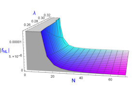
(a)

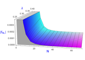
(b)

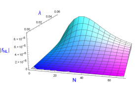
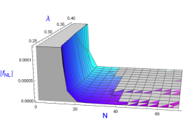
Figure 1: We show the behavior of the $f_{\rm NL}$ parameter for the perturbative, polynomial and exponential clases respectively, all of them showing a small value for the non-Gaussianity parameter

In all cases we calculate the value for the speed of sound, as a propagating speed for the scalar perturbations as discussed in Appendix A. The condition $c_{s}^{2}>0$ is fulfilled in all cases, showing that the model is free of pathologies.

3.1 Perturbative class

The most direct way to write a small parameter $\epsilon_{1}$ as a function of the large number of $e$-folds $N$, is the inverse relation, also called the perturbative class, is

$$\epsilon_{1}=\frac{\lambda}{N}.$$ (3.1)

The family of inflationary potentials in this class is recovered from integrating Eq. (2.13); that is, $V=V_{0}N^{2\lambda}$. The potential with the usual $T$ dependence and parametrized depending on the value of $\lambda$ reads:

$$V(T)=\widehat{V_{0}}T^{\frac{4\lambda}{1-2\lambda}}=\begin{cases}\quad\widehat{V_{0}}T^{n}&\quad 0<\lambda<\frac{1}{2},\\ \\ \quad V_{0}\exp\left(\sqrt{8\pi V_{0}}T\right)&\quad\lambda=\frac{1}{2},\\ \\ \quad\widehat{V_{0}}T^{-n}&\quad\frac{1}{2}<\lambda<\frac{3N}{2},\end{cases}$$ (3.2)

where $\widehat{V_{0}}=V_{0}\left[\frac{\pi\left(1-2\lambda\right)^{2}}{\lambda}\right]^{{\frac{2\lambda}{\left(1-2\lambda\right)}}}$ and $n=\mid\frac{4\lambda}{1-2\lambda}\mid$. We immediately see that from this perturbative class the monomial power law potential is recovered for $\lambda<\frac{1}{2}$. In particular, the quadratic and quartic forms, widely analyzed in the literature (e.g. [9, 11] and references therein), are recovered in this class of the large-$N$ formalism. The upper bound $\lambda=\frac{3}{2}N$ in the third family of potentials is set to guarantee that the effective sound speed $c_{s}$ be well defined. Indeed, for this class of models is given by

$$c_{s}^{2}={1-\frac{2\lambda}{3N}},$$ (3.3)

which limits the range of values of $\lambda$ in Eq. (3.2).

$V(T)\sim$	$\lambda$	$n_{s}$	$n_{t}$	$r$	$c_{s}$	$\mid{f_{\rm NL}}\mid$
$T^{2}$	$0.25$	$0.9699$	$-0.0101$	$0.0787$	$0.9983$	$1.6\times 10^{-7}$
$T^{4}$	$0.3333$	$0.9665$	$-0.0134$	$0.1048$	$0.9977$	$4.9\times 10^{-8}$
$T^{6}$	$0.375$	$0.9648$	$-0.0151$	$0.1179$	$0.9974$	$2\times 10^{-8}$
$T^{8}$	$0.4$	$0.9637$	$-0.0162$	$0.1258$	$0.9973$	$1\times 10^{-8}$
$\exp\left(\sqrt{8\pi V_{0}}T\right)$	$.05$	$0.9595$	$-0.0203$	$0.1571$	$0.9966$	$0$

Table 1: Values of the observables are here given for potentials determined by the parameter $\lambda$ in the perturbative class, up to second order in the Hubble flow parameters and at $N=50$ $e$-folds of inflation.

The spectral index, the tensor-to-scalar ratio, as well as the scalar and tensor runnings to second order in slow–roll can be derived from Eqs. (2.14) to (2.16). Explicitly,

$$r=\frac{16\lambda}{N}+\frac{\left(C-\frac{1}{3}\lambda\right)}{N^{2}},\qquad n_{s}=1-\frac{1+2\lambda}{N}-\frac{2\lambda(\lambda+2C+\frac{8}{3})}{N^{2}},\qquad n_{t}=-\frac{2\lambda}{N}-\frac{2\lambda(\lambda+2C+1)}{N^{2}}.$$ (3.4)

When evaluating the observables at $N=50$ we obtain the cosmological parameters values given in Table 1. Note that for the perturbative class we obtain values for $r$ small enough to meet the Bicep2/Keck/Planck constraints. The numerical values of cosmological parameters will appreciably change when varying $N$, an shown in Section 4.

In a rough comparison between the CSFI and TSFI scenarios within the perturbative class, we note that even at first order there are differences between the numerical values of the cosmological parameters between both models (see Table 2). On the other hand, the difference between the consistency relations of Eqs. (2.18) and (2.19) shows that

$$\Delta n_{t}\equiv n^{CSFI}_{t}-n^{TSFI}_{t}=-\frac{r}{48}$$ (3.5)

If future experiments measure the tensor-to-scalar ratio and the tensor index, a precision of order $1/50$ is required in the latter with respect to the face value of $r$ in order to distinguish between the CSFI and TSFI scenarios. Regarding the differences kept in other observables, we show in the next section that TSFI provides a better fit to the current data than the CSFI.

$V(T)$ vs $V(\phi)$	$n_{s\,{1}}(T)$	$n_{s\,{1}}(\phi)$	$\mid{n_{s\,{1}}(T)-n_{s\,{1}}(\phi)}\mid$	$r_{1}(T)$	$r_{1}(\phi)$	$\mid{r_{1}(T)-r_{1}(\phi)}\mid$
$T^{2}~{}~{}\text{vs}~{}~{}\phi^{2}$	$0.97$	$0.96$	$0.01$	$0.08$	$0.16$	$0.08$
$T^{4}~{}~{}\text{vs}~{}~{}\phi^{4}$	$0.9666$	$0.94$	$0.02668$	$0.10656$	$0.32$	$0.21344$
$T^{6}~{}~{}\text{vs}~{}~{}\phi^{6}$	$0.965$	$0.92$	$0.045$	$0.12$	$0.48$	$0.36$
$T^{8}~{}~{}\text{vs}~{}~{}\phi^{8}$	$0.964$	$0.9$	$0.064$	$0.128$	$0.64$	$0.512$

Table 2: Comparison between the canonical single field (CSFI) and the tachyonic (TSFI) inflationary scenarios. Cosmological parameters at first order are evaluated for $N=50$ $e$-folds of inflation.

The non-Gaussianity parameter for the perturbative class of models is given in the local limit by

$$f_{\rm NL}=\frac{\left(1-2\lambda\right)^{2}}{3N^{2}}\ln\left(\frac{1-2\lambda+2N}{2N}\right).$$ (3.6)

The amplitude of non-Gaussianity is plotted in Figure 1(a). As the equation above shows, $f_{\rm NL}$ is small since it behaves like $\frac{1}{N^{2}}$, regardless of the value of $\lambda$. Thus, for large-$N$, $f_{\rm NL}$ will always present negligible values.

3.2 Polynomial class

The polynomial class is characterized by an equation of state parameter given by

$$\epsilon_{1}=\frac{\lambda}{N(N^{2\lambda}+1)}.$$ (3.7)

While previous works have dismissed this class of models, arguing that sub-leading terms in the denominator provide a negligible contribution, here we show sensible differences can be distinguished between this and the previous perturbative class.

The family of inflationary potentials in this class is takes the form $V=V_{0}\frac{N^{2\lambda}}{N^{2\lambda}+1}$. Consequently, the potential as a function of $T$ is shown in the equation below depending on the value of $\lambda$

$$V(T)=\left[V_{0}-\frac{1}{\left(\frac{\pi V_{0}\left(1-2\lambda\right)^{2}}{\lambda}\right)^{{\frac{2\lambda}{\left(1-2\lambda\right)}}}T^{\frac{4\lambda}{1-2\lambda}}+1}\right]=\begin{cases}V_{0}\frac{AT^{n}}{AT^{n}+1}&\!\!\!\!\!\!\!\!\!\!\!\!\quad 0<\lambda<\frac{1}{2},\\ \\ \small{\frac{1}{2}V_{0}\left[1+\tanh\left(\sqrt{2\pi V_{0}}T\right)\right]}&\!\quad\lambda=\frac{1}{2},\\ \\ V_{0}\frac{A}{A+T^{n}}&\!\quad\lambda>\frac{1}{2},\end{cases}$$ (3.8)

where $A=\left[\frac{V_{0}\pi\left(1-2\lambda\right)^{2}}{\lambda}\right]^{{\frac{2\lambda}{\left(1-2\lambda\right)}}}$ and $n=\mid\frac{4\lambda}{1-2\lambda}\mid$. To our knowledge, this class of potentials has not been explored in previous studies of Tachyonic Inflation. While the effective sound speed $c^{2}_{s}=1-\frac{2}{3}\epsilon_{1}$ is a real number regardless of values for $\lambda$ in a realistic model. Computed up to second order in the Hubble flow parameters (up to $\mathcal{O}(\epsilon_{i}^{3})$), the values for the spectral and tensor indices and the tensor to scalar ratio are

$$n_{s} = -\left[\frac{3(C+N-N^{2})(1+N^{2\lambda})^{2}+2\lambda^{2}\left[3+2N^{2\lambda}\left(8+3C-2\right)\right]}{N^{2}\left(1+N^{2\lambda}\right)^{2}}\right]$$

$$- \left[\frac{2\lambda\left(1+N^{2\lambda}\right)\left[8+6C+3N+3N^{2\lambda}(C+N)\right]}{N^{2}\left(1+N^{2\lambda}\right)^{2}}\right],$$

$$n_{t} = \frac{-2\lambda\left(1+\lambda+C+N\right)-2\lambda N^{2\lambda}\left[1+C+2\lambda(1+C)+N\right]}{N^{2}\left(1+N^{2\lambda}\right)^{2}},$$

$$r = \frac{16\lambda\left[-\lambda+3(N+C)+3N^{2\lambda}\left(C+2\lambda C+N\right)\right]}{3N^{2}\left(1+N^{2\lambda}\right)^{2}}.$$ (3.9)

$V(T)\sim$	$\lambda$	$n_{s}$	$n_{t}$	$r$	$c_{s}$	$\mid{f_{\rm NL}}\mid$
$\frac{AT^{2}}{AT^{2}+1}$	$0.25$	$0.9703$	$-0.0012$	$0.0097$	$0.9997$	$2.2\times 10^{-6}$
$\frac{AT^{4}}{AT^{4}+1}$	$0.3333$	$0.967$	$-0.0009$	$0.0071$	$0.9998$	$3\times 10^{-6}$
$\frac{AT^{6}}{AT^{6}+1}$	$0.375$	$0.9654$	$-0.0007$	$0.0059$	$0.9998$	$3.4\times 10^{-6}$
$\frac{AT^{8}}{AT^{8}+1}$	$0.4$	$0.9644$	$-0.0006$	$0.0052$	$0.9998$	$3.7\times 10^{-6}$
$\!\!\!\!\!\!1\!\!\!~{}+\!\tanh\!\left(\!\sqrt{2\pi V_{0}}T\right)$	$0.5$	$0.9605$	$-0.0003$	$0.003$	$0.9999$	$4.8\times 10^{-6}$

Table 3: Values for observables in the polynomial class at second order in the Hubble flow parameters for the some $\lambda$ values for $N=50$ $e$-folds of inflation.

Numerical results for observables for $N=50$ are given in Table 3. Finally, the non-Gaussianity parameter for this class is

$$f_{\rm NL}=\left[\frac{(1-2\lambda)^{2}+N^{4}\lambda(1+2\lambda)-2N^{2\lambda}\left(\lambda+6\lambda^{2}-1\right)}{3N^{2}\left(1+N^{2\lambda}\right)^{2}}\right]\ln\left(1-\frac{2\lambda}{N(1+N^{2\lambda})}+\frac{1+2\lambda}{2N}\right).$$ (3.10)

As in the case of the perturbative class, Figure 1(b) shows that $f_{\rm NL}$ is small and asymptotically vanishing like $\frac{\lambda}{N(N^{2\lambda}+1)}$.

3.3 Exponential class

As a final example of the versatility of the large-$N$ formalism, we present two specific cases where the explicit form of the potential in terms of the field can be obtained. From the first case we recover a potential previously found in Refs. [25, 3, 8] for a tachyon inflationary model. The results obtained here complement those studies and provide important constraints on their parameters. In the second case we find a potential of the eternal inflation type. In both cases all the observable parameters are computed explicitly.

3.3.1 First exponential case

The first class is characterized by an equation of the state parameter given by

$$\epsilon_{1}=\frac{\lambda}{2\left(e^{\lambda N}+1\right)}.$$ (3.11)

The family of inflationary potentials in this class is integrated as $V=V_{0}\frac{e^{\lambda N}}{e^{\lambda N}+1}$, and the explicit form as a function of the tachyon field reads

$$V=\frac{V_{0}}{2\pi\lambda V_{0}T^{2}+1}.$$ (3.12)

The effective speed of sound and the values for the observables up to order $\mathcal{O}(\epsilon_{i}^{3})$ in the Hubble flow parameters are given by

$$c_{s}^{2} = {1-\frac{\lambda}{3\left(e^{\lambda N}+1\right)}},$$ (3.13)

$$n_{s} = 1-\lambda-\frac{\lambda^{2}\left[-3-2e^{\lambda N}(8+3C)\right]}{6(1+e^{\lambda N})^{2}}+\mathcal{O}(\epsilon_{i}^{3}),$$

$$n_{t} = -\frac{\lambda\left[2+\lambda+2(1+\lambda+\lambda C)e^{\lambda N}\right]}{(1+e^{\lambda N})^{2}}+\mathcal{O}(\epsilon_{i}^{3}),$$

$$r = \frac{4\lambda\left[6-\lambda+6(1+\lambda C)e^{\lambda N}\right]}{3\left(1+e^{\lambda N}\right)^{2}}+\mathcal{O}(\epsilon_{i}^{3}).$$

From plotting the non-Gaussianity parameter,

$$f_{\rm NL}=\frac{\lambda^{2}(1-3e^{\lambda N})\text{log}\left(1+\frac{\lambda}{2}\text{tanh}\left(\frac{\lambda N}{2}\right)\right)}{3\left(1+e^{\lambda N}\right)^{2}},$$ (3.14)

we note that the $f_{\rm NL}$ shows a peak for $N\sim 30$ and then vanishes asymptotically (Figure 1), while the value for the first non-Gaussianity parameter is again small, this might be a feature worth exploring for the cases where $f_{\rm NL}$ could be large.

3.3.2 Second exponential case

The second class is characterized by the following equation of the state parameter

$$\epsilon_{1}=\frac{2\lambda}{e^{2\lambda N}-e^{-2\lambda N}}.$$ (3.15)

The family of potentials $V=V_{0}\tanh(\lambda N)$, given in terms of $V(T)$ is

$$V=V_{0}\,\frac{1}{\cosh\left(\sqrt{8\pi\lambda V_{0}}T\right)}.$$ (3.16)

This is one of the most popular models in the literature, [e.g. 6, 7]. While our approach derives potentials from expressions of $\epsilon_{1}$, we show below that our analysis and subsequent fit to observations can contribute to constrain models inspired in string theory [7].

In this class the effective sound speed and observables up to order $\mathcal{O}(\epsilon_{i}^{3})$ in the Hubble parameter are

$$c_{s}^{2} = {1-\frac{2}{3}\lambda\,\text{csch}(2\lambda N)},$$ (3.17)

$$n_{s} = 1-\lambda\,\text{csch}^{2}(2\lambda N)\left[\frac{4}{3}\lambda(8+6C)\cosh(2\lambda N)+2(\lambda+2\lambda C+\sinh(2\lambda N))+\sinh(4\lambda N)\right],$$

$$n_{t} = -2\lambda\,\text{csch}(2\lambda N)\left[1+2\lambda(1+C)\coth(2\lambda N)+\lambda\,\text{csch}(2\lambda N)\right],$$

$$r = 16\lambda\,\text{csch}(2\lambda N)\left[1+2\lambda\coth(2\lambda N)-\frac{1}{3}\lambda\,\text{csch}(2\lambda N)\right].$$

If we take this results and evaluate for $N=50$ we obtain the cosmological parameters values given in Table 4. The non-Gaussianity for this class is

$$f_{\rm NL}=-\frac{4}{3}\lambda^{2}\,\text{sech}^{2}(\lambda N)\ln\left[1+\lambda\tanh(\lambda N)\right],$$ (3.18)

with $f_{\rm NL}$ again small as shown in Figure 1.

$V(T)\sim$	$\lambda$	$n_{s}$	$n_{t}$	$r$	$c_{s}$	$\mid{f_{\rm NL}}\mid$
$\!\!\!\,\frac{1}{\cosh\left(\sqrt{8\pi\lambda V_{0}}T\right)}$	$1\times 10^{-7}$	$0.9595$	$-0.0203$	$0.1571$	$0.9966$	$6.6\times 10^{-27}$
$\frac{1}{2\pi\lambda V_{0}T^{2}+1}$	$.04$	$0.9596$	$-0.0048$	$0.0371$	$0.9992$	$2.4\times 10^{-6}$

Table 4: Observables in both cases of the exponential class of models, at second order in the Hubble flow parameters, for $N=50$ $e$-folds of inflation.

4 Cosmological Parameters Vs Observations

4.1 Parameter fitting

We have used a suite of cosmological data to compare different models with observations. In Figure 2 we present the marginalized confidence regions at 68% and 95% on the pair of parameters $(n_{s},\,r)$ from two sets of observations. The red contours correspond to the confidence regions obtained from CMB data from the Planck satellite [26] plus BAO data from different observations at redshifts $z=0.106,0.15,0.57$ and $0.32$. We employed the 2015 Planck data release including TT, TE, EE, low P and lensing data. On the other hand, the blue contours correspond to baseline and lensing Planck data combined with Bicep2/Keck/Planck joint constraints on B-mode polarization [17].

For both datasets we used the publicly available Markov chains from Planck, analyzed by using python scripts from CosmoMC [27]. These chains were produced considering $n_{s}$, $n_{sk}$ and $r$ as free parameters. The primordial scalar power spectrum is determined by $A_{s}$, $n_{s}$ and $n_{sk}$, while the primordial tensor power spectrum will have an amplitude determined by $r$, with $n_{t}$ satisfying the consistency relation (2.19) at first order.

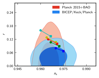
(a) The inflation models correspond to the perturbative class with potentials $V\propto T^{2}$ (blue), $T^{4}$ (green), $T^{6}$ (red), $T^{8}$ (yellow), and $e^{\sqrt{8\pi V_{0}}T}$ (cyan).

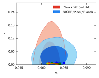
(b) The inflation models correspond to the polynomial class with potentials $V\propto~{}AT^{n}/(AT^{n}+1)$ for $n=2$ (blue), $n=4$ (green), $n=6$ (red), and $n=8$ (yellow).

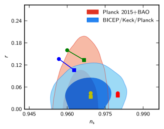
(c) Inflation models corresponding to the exponential classes. The potentials are $V\propto 1/\cosh(\sqrt{8\pi\lambda}T)$ for $\lambda=0.01$ (blue), and $\lambda=10^{-7}$ (green). Also $V=V_{0}/(2\pi\lambda V_{0}T^{2}+1)$ for $\lambda=0.02$ (red), and $\lambda=0.0307$ (yellow), see Table 4.

Figure 2: Marginalized confidence regions at $68\%$ and $95\%$ for $n_{s}$ and $r$ for the different classes of potentials in tachyon inflation. The blue region corresponds to Planck 2015 TT, low P and lensing data [26] plus the BICEP2/Keck/Planck collaboration data [17]. The red region represents Planck 2015 TT, TE, EE, low P and lensing confidence regions [26] including BAO from ref. [18]. $\blacksquare$ indicates evaluation of models at $N=60$ and thick coloured lines denote intermediate values up to the lower value $N=50$, represented by $\bullet$.

The results of our parameter analysis are condensed in Figure 2. From the Markov chains we obtain the primordial power spectrum parameters to have values of $n_{s}=0.966\pm 0.008$, $n_{sk}=-0.008\pm 0.015$ and $r<0.17$ at 95% confidence for the Planck 2015 plus BAO data and $n_{s}=0.968\pm 0.008$, $n_{sk}=-0.007\pm 0.015$ and $r<0.11$ at 95% confidence for the BICEP2/Keck/Planck data. In the leftmost panel, Figure 2(a), the perturbative class is reported. The model with exponential potential $e^{\sqrt{8\pi\lambda V_{0}}T}$ (corresponding to $\lambda=1/2$) is excluded at 95% confidence for the BICEP2/Keck/Planck data. In the same panel, the models corresponding to potentials of the form $V(T)\propto T^{4}$, $T^{6}$ and $T^{8}$ fall outside the 68% confidence region of both data sets. Such tension might increase with future CMB polarization observations. In the rightmost panel, Figure 2(b), we see that all the polynomial models studied fall inside the 68% confidence region of both datasets, at least for some values of $N$. This is thanks to the small amplitude of the tensor perturbations, generic in this class of models. In the bottom panel, Figure 2(c), we note that for the exponential models, and depending on the number of $e$-folds, a single potential can generate values that fall outside the 95% confidence region (for $N=50$) and values that almost reach the 68% confidence region for the Planck 2015 + BAO data (for $N=60$). The model with potential $V=V_{0}/(2\pi\lambda V_{0}T^{2}+1)$ lies precisely at the centre of both confidence regions if $\lambda=0.0307$.

4.2 An example from String Theory

As mentioned earlier, a popular model of Tachyon Inflation is that of Eq. (3.16), with its observational parameters constrained in Figure 2(c). Now we show that our results may serve to constrain also specific models derived from string theory. As a particular example, we look at the action (with restored Natural units for clarity)[7],

$$S=\int d^{4}x\sqrt{-g}\left[\frac{M_{\rm Pl}^{2}}{2}R-\mathcal{A}\tilde{V}(\tilde{T})\left(1+\mathcal{B}g^{\mu\nu}\partial_{\mu}\tilde{T}\partial_{\nu}\tilde{T}\right)^{1/2}\right],$$ (4.1)

where the potential of Eq. (3.16) written in terms of the fundamental string length $l_{s}=\sqrt{\alpha^{\prime}}$:

$$\tilde{V}(T)=\frac{\tilde{V}_{0}}{\cosh\left(\tilde{T}/\sqrt{2\alpha^{\prime}}\right)},$$ (4.2)

The extra parameters $\mathcal{A}$ and $\mathcal{B}$ are dimensionless numbers coming from the dimensional reduction of the action for the unstable brane system in string theory [7]. We note that our approach can constrain such numbers if we equate $V_{0}=\mathcal{A}\tilde{V}_{0}$, $T=\sqrt{\mathcal{B}}\tilde{T}$ and our parameter $\lambda=\tilde{\lambda}/(\mathcal{AB})$, when we express (4.2) in the form of (3.16) by writing,

$$x=\frac{\tilde{T}}{\sqrt{2\alpha^{\prime}}}={\tilde{T}\sqrt{\tilde{\lambda}\tilde{V}_{0}/M_{\rm Pl}^{2}}}=T\sqrt{\lambda{V}_{0}/M_{\rm Pl}^{2}}.$$ (4.3)

After these substitutions, the model in (4.1), (4.2) recovers the expressions in Eqs. (2.1) and (3.16). Our fit to observables yields parameter values derived from the set $[V_{0},\,\lambda,\,T(N=60)]=[3.37\times 10^{-9}M_{\rm Pl}^{4},0.01,2.12\times 10^{5}/M_{\rm Pl}]$, which consequently constrain the product

$$\alpha^{\prime}\mathcal{B}=\frac{M_{\rm Pl}^{2}}{2V_{0}\lambda}=1.48\times 10^{10}/M_{\rm Pl}^{2}.$$ (4.4)

Thus a given choice of the fundamental string length $\alpha^{\prime}$ is bound to generate a specific value of $\mathcal{B}$. In turn, this would set the value of the tachyon field of the string-inspired model with $\tilde{T}(N={60})=T(N={60})/\sqrt{\mathcal{B}}$. This would aid to reduce the value of the field trajectory during the inflationary stage; a desirable property to be explored in a follow-up paper [28]. Further constraints to this particular model involve values for the radius of compactification (see [29, 7]), a subject to be explored elsewhere. For now, this example demonstrates that our analysis can constrain models motivated by high energy physics, with the bonus of a physical interpretation for our auxiliary parameter $\lambda$.

5 Discussion and Concluding Remarks

We have studied the tachyon field inflationary scenario by means of the large-$N$ formalism. We propose three universal classes of models for this scenario; namely the perturbative, polynomial and exponential classes, presented in Section 3. Such classification is naturally derived within the large-$N$ formalism and allows us to organize different models for the tachyon field inflation scenario in terms of their cosmological predictions, in the large-$N$ limit. A family of potentials is obtained for each one of the classes, with every realization corresponding to a numerical value of the parameter $\lambda$. We calculate for all the classes the form of the cosmological parameters in terms of the number of $e$-folds.

In the first case of study, the perturbative class, we recover the well known family of power-law potentials. We report on constraints to some of the most important realizations of the model through up-to-date observations. This first class of models is particularly important since we can directly compare the models of Tachyon Scalar Field Inflation (TSFI) with those reconstructed for the Canonical Scalar Field Inflation (CSFI) scenario by means of their respective consistency relations, Eqs. (2.19) and (2.18), respectively. We find sensible differences in the results for the tensor-to-scalar ratio (see Eq. (3.5)). We conclude that a precision of order one in $50$ in the detection of the tensor index with respect to a hypothetically observed value of the tensor-to scalar ratio is required in order to distinguish both scenarios.

For the second class of models, the polynomial class, we have derived a novel family of potentials within the tachyon inflationary scenario (see Eq. (3.8)). The corresponding results in Figure 2(b) show that the polynomial class accommodates models that better fit the data, and mostly prefer a very small value of the tensor-to-scalar ratio.

For the exponential class, we focus on two specific cases for which we can derive an explicit function of the potential $V(T)$. From both cases we find cases theoretically motivated in previous studies [25, 3, 8, 6, 7]. The results obtained here complement previous analyses and provide a method to constrain those models.

We estimate higher order contributions of the inflationary perturbations by computing the non-Gaussianity parameter $f_{\rm NL}$ for the perturbations of the tachyon field model. In all cases this parameter in the local configuration approaches asymptotically to zero for large $N$, leading to a Gaussian distribution in the large-$N$ limit.

As argued in previous studies, high precision will be required in observations to distinguish tachyon inflation from its canonical counterpart. In particular, we note that the main differences arise for the cosmological parameters at second order in slow–roll. This is the main motivation to report the expressions of cosmological parameters at this order for each class. However, the difference between both scenarios at large $N$, where the featured formalism is valid, shows to be negligible.

The main feature of our study is the possibility of determining the observable parameters for several classes of potentials within the Tachyon inflationary scenario, by exploiting the large-$N$ formalism. The results in Figure 2 display important differences between the various realizations of the models in three classes of potentials. We conclude that the large-$N$ formalism is a powerful method to explore the richness of inflationary scenarios and to address their viability with enough precision for present and future observations.

Appendix A The Fluid Approximation

The fluid description of the tachyon field is valid as long as its evolution follows an adiabatic path. In the background such trajectory is derived from the first law of thermodynamics and implies the continuity equation. The stability of the adiabatic description is tested through perturbations and we show here that the non-adiabatic perturbations are suppressed in the inflationary stage.

The density and pressure of the tachyon field can be read from the matter action as

$$\rho_{T}=\frac{V(T)}{\sqrt{1-\dot{T}^{2}}},\quad P_{T}=-{V(T)}{\sqrt{1-\dot{T}^{2}}}.$$ (A.1)

The adiabatic trajectory is one where the pressure and density change proportionally, according to the equation of state

$$w\equiv\frac{P}{\rho}=-1+\dot{T}^{2},$$ (A.2)

which can be written in terms of the first Hubble flow parameter,

$$\epsilon_{1}(N)=-\frac{\dot{H}}{H^{2}}=\frac{3}{2}\left(1+\frac{P}{\rho}\right)=\frac{3}{2}\left(1+\omega\right).$$ (A.3)

It is because of this last equivalence that the first Hubble flow slow–roll parameter $\epsilon_{1}(N)$ has been dubbed the equation of state parameter. Yet the trajectories of the tachyon field may deviate from adiabaticity, which would break the fluid approximation for the tachyon perturbations. Here we show that this is not the case by looking at the adiabatic sound speed. This is the speed of perturbations along the adiabatic trajectory, and is given by

$$c_{s}^{2}\equiv\frac{\dot{P_{T}}}{\dot{\rho}_{T}}=-w\left(1+\frac{2}{3}\frac{(\ln{V})^{\prime}}{H\dot{T}}\right).$$ (A.4)

This is easily derived from the continuity equation and the Hamilton-Jacobi Eq. (2.9). For matter perturbations, the departure from adiabaticity is denoted by the entropy perturbation $\delta P_{\rm nad}$:

$$\delta P_{T}=c_{s}^{2}\delta\rho_{T}+\delta P_{\rm nad}=c_{s}^{2}\delta\rho_{T}+P_{T}\Gamma.$$ (A.5)

Here $\Gamma$, the entropy perturbation, parametrizes the difference between uniform density and uniform pressure slices. That is,

$$P_{T}\Gamma\equiv(c_{\rm eff}^{2}-c_{s}^{2})\delta\rho_{\rm com}=\frac{2}{3}\frac{(\ln{V})^{\prime}}{H\dot{T}}\delta\rho_{\rm com}\,,\qquad\quad\mathrm{with}\quad c_{\rm eff}\equiv\frac{\partial P_{T}}{\partial\dot{T}}/\frac{\partial\rho_{T}}{\partial\dot{T}}=w.$$ (A.6)

Here we introduced the effective sound speed $c_{\rm eff}=w$, and note that the sub-index _com indicates that the matter density is measured in hypersurfaces orthogonal to world lines comoving with the fluid (comoving gauge). The comoving energy density perturbation is related to the gauge-invariant Bardeen metric potential $\Psi_{B}$ through the Poisson equation [30, 31],

$$4\pi Ga^{2}\delta\rho_{\rm com}=\nabla^{2}\Psi_{B}.$$ (A.7)

a field equation valid even in a fluid with non-vanishing pressure [32]. On the other hand, the difference in sound speeds can be written in terms of the slow–roll parameters defined in (2.6),

$$c_{\rm eff}^{2}-c_{s}^{2}=\frac{2}{3}\frac{(\ln{V})^{\prime}}{H\dot{T}}=-2-\frac{2}{3}\frac{\epsilon_{2}}{(1+\frac{2}{3}\epsilon_{1})}.$$ (A.8)

Combining the last two expressions we can write

$$\Gamma=-\frac{1}{w\rho_{T}}\left(2+\frac{2}{3}\frac{\epsilon_{2}}{(1+\frac{2}{3}\epsilon_{1})}\right)\frac{\nabla^{2}\Psi_{B}}{4\pi Ga^{2}}=\frac{4}{3}\left(1+\frac{1}{3}\frac{\epsilon_{2}}{(1+\frac{2}{3}\epsilon_{1})}\right)\frac{\nabla^{2}\Psi_{B}}{a^{2}H^{2}}.$$ (A.9)

The factor in large brackets is of order one in a slow–roll inflationary regime. However, inflationary perturbations are generated at horizon exit and subsequently expand to scales well above the Hubble horizon $r_{H}=1/H$, which implies that $\nabla^{2}/(aH)^{2}\ll 1$. The entropy perturbations are thus suppressed in the usual inflationary picture. This result agrees with that found in [8] and justifies our assumption of adiabatic fluctuations when computing spectra and the bispectrum of the tachyon field.

References

- [1] A.H. Guth, “The Inflationary Universe: A possible solution to the horizon and flatness problems,”Phys. Rev. D23 (1981) 347. A.D Linde, “A New Inflationary Universe Scenario: A Possible Solution of the Horizon, Flatness, Homogeneity, Isotropy and Primordial Monopole Problems,” Phys. Lett. B108 (1982) 389. A. Albrecht and P.J. Steinhardt, “ Cosmology for Grand Unified Theories with Radiatively Induced Symmetry Breaking,” Phys. Rev. Lett. 48 (1982) 1220. D. H. Lyth and A. Riotto, “Particle physics models of inflation and the cosmological density perturbation,” Phys. Rept. 314 (1999) 1 [hep-ph/9807278]. D. H. Lyth and A. R. Liddle, “The primordial density perturbation: Cosmology, inflation and the origin of structure,” Cambridge, UK: Cambridge Univ. Pr. (2009) 497 p. D. Baumann, “TASI Lectures on Inflation,” [arXiv:0907.5424 [hep-th]].
- [2] A. Sen, “BPS D-branes on nonsupersymmetric cycles,” JHEP 9812 (1998) 021 [hep-th/9812031]. A. Sen, “Supersymmetric world volume action for nonBPS D-branes,” JHEP 9910 (1999) 008 [hep-th/9909062]. A. Sen, “Tachyon condensation on the brane anti-brane system,” JHEP 9808 (1998) 012 [hep-th/9805170]. A. Sen, “Tachyon matter,” JHEP 0207 (2002) 065 [hep-th/0203265]. A. Sen, “Rolling tachyon,” JHEP 0204 (2002) 048 [hep-th/0203211].
- [3] A. Sen, “Field theory of tachyon matter,” Mod. Phys. Lett. A 17 (2002) 1797 [hep-th/0204143].
- [4] G. German, A. Herrera-Aguilar, D. Malagon-Morejon, R. R. Mora-Luna and R. da Rocha, “A de Sitter tachyon thick braneworld and gravity localization,” JCAP 1302 (2013) 035 [arXiv:1210.0721 [hep-th]].
- [5] G. W. Gibbons, “Cosmological evolution of the rolling tachyon,” Phys. Lett. B 537 (2002) 1 [hep-th/0204008].
- [6] F. Leblond and A. W. Peet, JHEP 0304 (2003) 048 [hep-th/0303035]. C. j. Kim, H. B. Kim, Y. b. Kim and O. K. Kwon, JHEP 0303 (2003) 008 [hep-th/0301076]. N. D. Lambert, H. Liu and J. M. Maldacena, JHEP 0703 (2007) 014 [hep-th/0303139].
- [7] D. Cremades, F. Quevedo and A. Sinha, “Warped tachyonic inflation in type IIB flux compactifications and the open-string completeness conjecture,” JHEP 0510 (2005) 106 [hep-th/0505252].
- [8] D. A. Steer and F. Vernizzi, “Tachyon inflation: Tests and comparison with single scalar field inflation,” Phys. Rev. D 70, 043527 (2004) [hep-th/0310139].
- [9] K. Nozari and N. Rashidi, “Some Aspects of Tachyon Field Cosmology,” Phys. Rev. D 88 (2013) 2, 023519 [arXiv:1306.5853 [gr-qc]].
- [10] S. Li and A. R. Liddle, “Observational constraints on tachyon and DBI inflation,” JCAP 1403, 044 (2014) [arXiv:1311.4664 [astro-ph.CO]].
- [11] K. Nozari and N. Rashidi, “Tachyon field inflation in light of BICEP2,” Phys. Rev. D 90, no. 4, 043522 (2014) [arXiv:1408.3192 [astro-ph.CO]].
- [12] D. Boyanovsky, H. J. de Vega and N. G. Sanchez, “Clarifying Inflation Models: Slow-roll as an expansion in ” Phys. Rev. D 73 (2006) 023008 [astro-ph/0507595].
- [13] D. Roest, “Universality classes of inflation,” JCAP 1401 (2014) 01, 007 [arXiv:1309.1285 [hep-th]].
- [14] J. Garcia-Bellido and D. Roest, “Large- running of the spectral index of inflation,” Phys. Rev. D 89 (2014) 10, 103527 [arXiv:1402.2059 [astro-ph.CO]].
- [15] V. Mukhanov, “Quantum Cosmological Perturbations: Predictions and Observations,” Eur. Phys. J. C 73 (2013) 2486 [arXiv:1303.3925 [astro-ph.CO]].
- [16] J. Garcia-Bellido, D. Roest, M. Scalisi and I. Zavala, “Can CMB data constrain the inflationary field range?,” JCAP 1409 (2014) 006 [arXiv:1405.7399 [hep-th]].
- [17] P. A. R. Ade et al. [BICEP2 and Planck Collaborations], “A Joint Analysis of BICEP2/Keck Array and Planck Data,” Phys. Rev. Lett. 114, no. 10, 101301 (2015) [arXiv:1502.00612 [astro-ph.CO]].
- [18] F. Beutler, C. Blake, M. Colless, D. H. Jones, L. Staveley-Smith, L. Campbell, Q. Parker and W. Saunders et al., “The 6dF Galaxy Survey: Baryon Acoustic Oscillations and the Local Hubble Constant,” Mon. Not. Roy. Astron. Soc. 416, 3017 (2011) [arXiv:1106.3366 [astro-ph.CO]]. A. J. Ross, L. Samushia, C. Howlett, W. J. Percival, A. Burden and M. Manera, “The Clustering of the SDSS DR7 Main Galaxy Sample I: A 4 per cent Distance Measure at z=0.15,” arXiv:1409.3242 [astro-ph.CO]. L. Anderson et al. [BOSS Collaboration], “The clustering of galaxies in the SDSS-III Baryon Oscillation Spectroscopic Survey: Baryon Acoustic Oscillations in the Data Release 10 and 11 galaxy samples,” Mon. Not. Roy. Astron. Soc. 441, 24 (2014); [arXiv:1312.4877 [astro-ph.CO]].
- [19] D. J. Schwarz, C. A. Terrero-Escalante and A. A. Garcia, “Higher order corrections to primordial spectra from cosmological inflation,” Phys. Lett. B 517 (2001) 243; [astro-ph/0106020].
- [20] M. Sasaki and E. D. Stewart, “A General analytic formula for the spectral index of the density perturbations produced during inflation,” Prog. Theor. Phys. 95, 71 (1996) [astro-ph/9507001].
- [21] P. Creminelli, A. Nicolis, L. Senatore, M. Tegmark and M. Zaldarriaga, “Limits on non-gaussianities from wmap data,” JCAP 0605 (2006) 004 [astro-ph/0509029].
- [22] E. Komatsu, “Hunting for Primordial Non-Gaussianity in the Cosmic Microwave Background,” Class. Quant. Grav. 27 (2010) 124010 [arXiv:1003.6097 [astro-ph.CO]].
- [23] P. A. R. Ade et al. [Planck Collaboration], “Planck 2015 results. XVII. Constraints on primordial non-Gaussianity,” arXiv:1502.01592 [astro-ph.CO].
- [24] J. E. Lidsey, A. R. Liddle, E. W. Kolb, E. J. Copeland, T. Barreiro and M. Abney, “Reconstructing the inflation potential : An overview,” Rev. Mod. Phys. 69 (1997) 373 [astro-ph/9508078].
- [25] M. Sami, P. Chingangbam and T. Qureshi, “Aspects of tachyonic inflation with exponential potential,” Phys. Rev. D 66 (2002) 043530 [hep-th/0205179].
- [26] R. Adam et al. [Planck Collaboration], “Planck 2015 results. I. Overview of products and scientific results,” [arXiv:1502.01582 [astro-ph.CO]].
- [27] A. Lewis and S. Bridle, “Cosmological parameters from CMB and other data: A Monte Carlo approach,” Phys. Rev. D 66, 103511 (2002) [astro-ph/0205436].
- [28] N. Barbosa-Cendejas, et al. In Preparation, 2015.
- [29] L. Kofman and A. D. Linde, “Problems with tachyon inflation,” JHEP 0207 (2002) 004 [hep-th/0205121].
- [30] J. M. Bardeen, “Gauge Invariant Cosmological Perturbations,” Phys. Rev. D 22 (1980) 1882.
- [31] D. Wands and A. Slosar, “Scale-dependent bias from primordial non-Gaussianity in general relativity,” Phys. Rev. D 79 (2009) 123507 [arXiv:0902.1084 [astro-ph.CO]].
- [32] A. J. Christopherson, J. C. Hidalgo and K. A. Malik, “Modelling non-dust fluids in cosmology,” JCAP 1301, 002 (2013) [arXiv:1207.1870 [astro-ph.CO]]