Framework for Multi-task Multiple Kernel Learning and Applications in Genome Analysis

Abstract

We present a general regularization-based framework for Multi-task learning (MTL), in which the similarity between tasks can be learned or refined using $\ell_{p}$-norm Multiple Kernel learning (MKL). Based on this very general formulation (including a general loss function), we derive the corresponding dual formulation using Fenchel duality applied to Hermitian matrices. We show that numerous established MTL methods can be derived as special cases from both, the primal and dual of our formulation. Furthermore, we derive a modern dual-coordinate descend optimization strategy for the hinge-loss variant of our formulation and provide convergence bounds for our algorithm. As a special case, we implement in C++ a fast LibLinear-style solver for $\ell_{p}$-norm MKL. In the experimental section, we analyze various aspects of our algorithm such as predictive performance and ability to reconstruct task relationships on biologically inspired synthetic data, where we have full control over the underlying ground truth. We also experiment on a new dataset from the domain of computational biology that we collected for the purpose of this paper. It concerns the prediction of transcription start sites (TSS) over nine organisms, which is a crucial task in gene finding. Our solvers including all discussed special cases are made available as open-source software as part of the SHOGUN machine learning toolbox (available at http://shogun.ml).

1 Introduction

One of the key challenges in computational biology is to build effective and efficient statistical models that learn from data to predict, analyze, and ultimately understand biological systems. Regardless of the problem at hand, however, be it the recognition of sequence signals such as splice sites, the prediction of protein-protein interactions, or the modeling of metabolic networks, we frequently have access to data sets for multiple organisms, tissues or cell-lines. Can we develop methods that optimally combine such multi-domain data?

While the field of Transfer or Multitask Learning enjoys a growing interest in the Machine Learning community in recent years, it can be traced back to ideas from the mid 90’s. During that time Thrun (1996) asked the provocative question ”Is Learning the $n$-th Thing any Easier Than Learning the First?”, effectively laying the ground for the field of Transfer Learning. Their work was motivated by findings in human psychology, where humans were found to be capable of learning based on as few as a single example (Ahn and Brewer, 1993). The key insight was that humans build upon previously learned related concepts, when learning new tasks, something Thrun (1996) call lifelong learning. Around the same time, Caruana (1993, 1997) coined the term Multitask Learning. Rather than formalizing the idea of learning a sequence of tasks, they propose machinery to learn multiple related tasks in parallel.

While most of the early work on Multitask Learning was carried out in the context of learning a shared representation for neural networks (Caruana, 1997; Baxter, 2000), Evgeniou and Pontil (2004) adapted this concept in the context of kernel machines. At first, they assumed that the models of all tasks are close to each other (Evgeniou and Pontil, 2004) and later generalized their framework to non-uniform relations, allowing to couple some tasks more strongly than others (Evgeniou et al., 2005), according to some externally defined task structure. In recent years, there has been an increased interest in learning the structure potentially underlying the tasks. Ando and Zhang (2005) proposed a non-convex method based on Alternating Structure Optimization (ASO) for identifying the task structure. A convex relaxation of their approach was developed by Chen et al. (2009). Zhou et al. (2011) showed the equivalence between ASO and Clustered Multitask Learning (Jacob et al., 2008; Obozinski et al., 2010) and their convex relaxations. While the structure between tasks is defined by assigning tasks to clusters in the above approaches, Zhang and Yeung (2010) propose to learn a constrained task covariance matrix directly and show the relationship to Multitask Feature Learning (Argyriou et al., 2007, 2008a, 2008b; Liu et al., 2009). Here, the basic idea is to use a LASSO-inspired (Tibshirani, 1996) $\ell_{2,1}$-norm to identify a subset of features that is relevant to all tasks.

A challenge remains to find an adequate task similarity measure to compare the multiple domains and tasks. While existing parameter-free approaches such as Romera-Paredes et al. (2013) ignore biological background knowledge about the relatedness of the tasks, in this paper, we present a parametric framework for regularization-based multitask learning that subsumes several approaches and automatically learns the task similarity from a set of candidates measures using $\ell_{p}$-norm Multiple Kernel learning (MKL) see, for instance, Kloft et al. (2011). We thus provide a middle ground between assuming known task relationships and learning the entire task structure from scratch. We propose a general unifying framework of MT-MKL, including a thorough dualization analysis using Fenchel duality, based on which we derive an efficient linear solver that combines our general framework with advances in linear SVM solvers and evaluate our approach on several datasets from Computational Biology.

This paper is based on preliminary material shown in several conference papers and workshop contributions (Widmer et al., 2010a, c, b, 2012; Widmer and Rätsch, 2012), which contained preliminary aspects of the framework presented here. This version additionally includes a unifying framework including Fenchel duality analysis, more complete derivations and theoretical analysis as well as a comparative study in multitask learning and genomics, where we brought together genomic data for a wide range of biological organisms in a multitask learning setting. This dataset will be made freely available and may serve as a benchmark in the domain of multitask learning. Our experiments show that combining data via multitask learning can outperform learning each task independently. In particular, we find that it can be crucial to further refine a given task similarity measure using multitask multiple kernel learning.

The paper is structured as follows: In Section 2 we introduce a unifying view of multitask multiple kernel learning that covers a wide range loss functions and regularizers. We give a general Fenchel dual representation and a representer theorem, and show that the formulation contains several existing formulations as special cases. In Section 3 we propose two optimization strategies: one that can be applied out of the box with any custom set of kernels and another one that is specifically tailored to linear kernels as well as string kernels. Both algorithms were implemented into the Shogun machine learning toolbox. In Section 4 we present results of empirical experiments on artificial data as well as a large biological multi-organism dataset curated for the purpose of this paper.

2 A Unifying View of Regularized Multi-Task Learning

In this section, we present a novel multi-task framework comprising many existing formulations, allowing us to view prevalent approaches from a unifying perspective, yielding new insights. We can also derive new learning machines as special instantiations of the general model. Our approach is embedded into the general framework of regularization-based supervised learning methods, where we minimize a functional

$${\mathfrak{R}}(\boldsymbol{w})+C\thinspace{\mathfrak{L}}(\boldsymbol{w})\thinspace,$$

which consists of a loss-term ${\mathfrak{L}}(\boldsymbol{w})$ measuring the training error and a regularizer ${\mathfrak{R}}(\boldsymbol{w})$ penalizing the complexity of the model $\boldsymbol{w}$. The positive constant $C>0$ controls the trade-off of the criterion. The formulation can easily be generalized to the multi-task setting, where we are interested in obtaining several models parametrized by $\boldsymbol{w}_{1},\ldots,\boldsymbol{w}_{T}$, where $T$ is the number of tasks.

In the past, this has been achieved by employing a joint regularization term ${\mathfrak{R}}(\boldsymbol{w}_{1},\ldots,\boldsymbol{w}_{T})$ that penalizes the discrepancy between the individual models (Evgeniou et al., 2005; Agarwal et al., 2010),

$${\mathfrak{R}}(\boldsymbol{w}_{1},\ldots,\boldsymbol{w}_{T})+C\thinspace{\mathfrak{L}}(\boldsymbol{w}_{1},\ldots,\boldsymbol{w}_{t})\thinspace.$$

A common approach is, for example, to set ${\mathfrak{R}}(\boldsymbol{w}_{1},\ldots,\boldsymbol{w}_{T})=\frac{1}{2}\sum\nolimits_{s,t=1}^{T}q_{st}\left\|\boldsymbol{w}_{s}-\boldsymbol{w}_{t}\right\|^{2}\thinspace,$ where $Q=\left(q_{st}\right)_{a\leq s,t\leq T}$ is a task similarity matrix. In this paper, we develop a novel, general framework for multi-task learning of the form

$$\min_{\boldsymbol{W},\theta}~{}{\mathfrak{R}}(\boldsymbol{W},{\boldsymbol{\theta}})+C{\mathfrak{L}}(\boldsymbol{W})\thinspace,$$

where $\boldsymbol{W}=(W_{m})_{1\leq m\leq M}$, $W_{m}=(\boldsymbol{w}_{m1},\ldots,\boldsymbol{w}_{mT})$. This approach has the additional flexibility of allowing us to incorporate multiple task similarity matrices into the learning problem, each equipped with a weighting factor. Instead of specifying the weighting factor a priori, we will automatically determine optimal weights from the data as part of the learning problem. We show that the above formulation comprises many existing lines of research in the area; this not only includes very recent lines but also seemingly different ones. The unifying framework allows us to analyze a large variety of MTL methods jointly, as exemplified by deriving a general dual representation of the criterion, without making assumptions on the employed norms and losses, besides the latter being convex. This delivers insights into connections between existing MTL formulations and, even more importantly, can be used to derive novel MTL formulations as special cases of our framework, as done in a later section of this paper.

2.1 Problem Setting and Notation

Let $D=\{(x_{1},y_{1}),\ldots,(x_{n},y_{n})\}$ be a set of training pattern/label pairs. In multitask learning, each training example $(x_{i},y_{i})$ is associated with a task $\tau(i)\in\{1,\ldots,T\}$. Furthermore, we assume that for each $t\in\{1,\ldots,T\}$ the instances associated with task $t$ are independently drawn from a probability distribution $P_{t}$ over a measurable space $\mathcal{X}_{t}\times\mathcal{Y}_{t}$. We denote the set of indices of training points of the $t$th task by $I_{t}:=\{i\in\{1,\ldots,n\}:\tau(i)=t\}$. The goal is to find, for each task $t\in\{1,\ldots,T\}$, a prediction function $f_{t}:\mathcal{X}\rightarrow{\mathbb{R}}$. In this paper, we consider composite functions of the form $f_{t}:x\mapsto\sum_{m=1}^{M}\langle\boldsymbol{w}_{mt},\varphi_{m}(x)\rangle$, $1\leq t\leq T$, where $\varphi_{m}:\mathcal{X}\rightarrow{\mathcal{H}}_{m}$, $1\leq m\leq M$, are mappings into reproducing Hilbert spaces ${\mathcal{H}}_{1},\ldots,{\mathcal{H}}_{M}$, encoding multiple views of the multi-task learning problem via kernels $k_{m}(x,\tilde{x})=\langle\varphi_{m}(x),\varphi_{m}(\tilde{x})\rangle$, and $\boldsymbol{W}:=(\boldsymbol{w}_{mt})_{1\leq m\leq M,\thinspace 1\leq t\leq T}$, $w_{mt}\in{\mathcal{H}}_{m}$ are parameter vectors of the prediction function.

For simplicity of notation, we concentrate on binary prediction, i.e., $\mathcal{Y}=\{-1,1\}$, and encode the loss of the prediction problem as a loss term ${\mathfrak{L}}(\boldsymbol{W}):=\sum_{i=1}^{n}l(y_{i}f_{\tau(i)}(x_{i}))$, where $l:\mathbb{R}\rightarrow{\mathbb{R}}\cup\{\infty\}$ is a loss function, assumed to be closed convex, lower bounded and finite at $0$. To consider sophisticated couplings between the tasks, we introduce so-called task-similarity matrices $Q_{1},\ldots,Q_{M}\in\textrm{GL}_{n}({\mathbb{R}})$ with $Q_{m}=(q_{mst})_{1\leq s,t\leq T}$,  $Q^{-1}_{m}=\big{(}q_{mst}^{(-1)}\big{)}_{1\leq s,t\leq T}$ and consider the regularizer ${\mathfrak{R}}_{{\boldsymbol{\theta}}}(\boldsymbol{W})=\frac{1}{2}\sum_{m=1}^{M}\|W_{m}\|^{2}_{Q_{m}}/\theta_{m}$ (setting $1/0:=\infty$, $0/0:=0$) with $\left\|W_{m}\right\|_{Q_{m}}:=\operatorname*{tr}(W_{m}Q_{m}W_{m}^{*})=\sqrt{\sum_{s,t=1}^{T}q_{mst}\left\langle\boldsymbol{w}_{ms},\boldsymbol{w}_{mt}\right\rangle}$, where $W_{m}=(\boldsymbol{w}_{m1},\ldots,\boldsymbol{w}_{mT})\in\bigoplus_{t=1}^{T}{\mathcal{H}}_{m}=:{\mathcal{H}}_{m}^{T}$ with adjoint $W_{m}^{*}$ and $\operatorname*{tr}(\cdot)$ denotes the trace class operator of the tensor Hilbert space ${\mathcal{H}}_{m}\otimes{\mathcal{H}}_{m}$. Note that also the direct sum ${\mathcal{H}}:=\bigoplus_{m=1}^{M}{\mathcal{H}}_{m}^{T}$ is a Hilbert space, which will allow us to view $\boldsymbol{W}\in{\mathcal{H}}$ as an element in a Hilbert space. The parameters ${\boldsymbol{\theta}}=(\theta_{m})_{1\leq m\leq M}\in\Theta_{p}$, $\Theta_{p}:=\{{\boldsymbol{\theta}}\in{\mathbb{R}}^{M}:\theta_{m}\geq 0,1\leq m\leq M,\left\|{\boldsymbol{\theta}}\right\|_{p}\leq 1\}$, are adaptive weights of the views, where $\left\|{\boldsymbol{\theta}}\right\|_{p}=\sqrt[p]{\sum_{m=1}^{M}|\theta_{m}|^{p}}$ denotes the $\ell_{p}$-norm. Here ${\boldsymbol{\theta}}\succeq\mathbf{0}$ denotes $\theta_{m}\geq 0$, $m=1,\ldots,M$.

Using the above specification of the regularizer and the loss term, we study the following unifying primal optimization problem.

Problem 1 (Primal problem).

Solve

$$\inf_{{\boldsymbol{\theta}}\in\Theta_{p},\boldsymbol{W}\in{\mathcal{H}}}\quad{\mathfrak{R}}_{{\boldsymbol{\theta}}}(\boldsymbol{W})~{}+~{}C\thinspace{\mathfrak{L}}\big{(}A(\boldsymbol{W})\big{)}\thinspace,$$

where

$${\mathfrak{R}}_{{\boldsymbol{\theta}}}(\boldsymbol{W}):=\frac{1}{2}\sum_{m=1}^{M}\frac{\|W_{m}\|^{2}_{Q_{m}}}{\theta_{m}}\thinspace,\quad\|W_{m}\|^{2}_{Q_{m}}:=\operatorname*{tr}(W_{m}Q_{m}W_{m}^{*})$$

$${\mathfrak{L}}(A(\boldsymbol{W})):=\sum_{i=1}^{n}l\big{(}A_{i}(\boldsymbol{W})\big{)}\thinspace,~{}~{}A(\boldsymbol{W}):=\left(A_{i}(\boldsymbol{W})\right)_{1\leq i\leq n}\thinspace,~{}~{}A_{i}(\boldsymbol{W}):=y_{i}\sum_{m=1}^{M}\big{\langle}\boldsymbol{w}_{m\tau(i)},\varphi_{m}(x_{i})\big{\rangle}\thinspace.$$

2.2 Dualization

Dual representations of optimization problems deliver insight into the problem, which can be used in practice to, for example, develop optimization algorithms (so done in Section 3 of this paper). In this section, we derive a dual representation of our unifying primal optimization problem, i.e., Problem 1. Our dualization approach is based on Fenchel-Rockafellar duality theory. The basic results of Fenchel-Rockafellar duality theory for Hilbert spaces are reviewed in Appendix A. We present two dual optimization problems: one that is dualized with respect to $\boldsymbol{W}$ only (i.e., considering ${\boldsymbol{\theta}}$ as being fixed) and one that completely removes the dependency on ${\boldsymbol{\theta}}$.

2.2.1 Computation of Conjugates and Adjoint Map

To apply Fenchel’s duality theorem, we need to compute the adjoint map $A^{*}$ of the linear map $A:{\mathcal{H}}\rightarrow{\mathbb{R}}^{n}$, $A(\boldsymbol{W})=\big{(}A_{i}(\boldsymbol{W})\big{)}_{1\leq i\leq n}$, as well as the convex conjugates of ${\mathfrak{R}}$ and ${\mathfrak{L}}$. See Appendix A for a review of the definitions of the convex conjugate and the adjoint map. First, we notice that, by the basic identities for convex conjugates of Prop. 10 in Appendix A, we have that

$$\big{(}C{\mathfrak{L}}({\boldsymbol{\alpha}})\big{)}^{*}~{}=~{}C{\mathfrak{L}}^{*}({\boldsymbol{\alpha}}/C)~{}=~{}C\Big{(}\sum\nolimits_{i=1}^{n}l(\alpha_{i}/C)\Big{)}^{*}~{}=~{}C\sum\nolimits_{i=1}^{n}l^{*}(\alpha_{i}/C)\thinspace.$$

Next, we define $A^{*}:{\mathbb{R}}^{n}\rightarrow{\mathcal{H}}$ by $A^{*}({\boldsymbol{\alpha}})=\big{(}\sum_{i\in I_{t}}\alpha_{i}y_{i}\varphi_{m}(x_{i})\big{)}_{1\leq m\leq M,1\leq t\leq T}$ . Recall that the mapping between tasks and examples may be expressed in one of two ways. We may use index set $I_{t}$ to retrieve the indices of training examples associated with task $t$. Alternatively, we may use task indicator $\tau(i)\in\{1,\dots,T\}$ to obtain the task index $\tau(i)$ associated with $i$th training example. Using this notation, we verify that, for any $\boldsymbol{W}\in{\mathcal{H}}$ and ${\boldsymbol{\alpha}}\in{\mathbb{R}}^{n}$, it holds

$$\left\langle\boldsymbol{W},A^{*}({\boldsymbol{\alpha}})\right\rangle = \Big{\langle}\big{(}w_{mt}\big{)}_{1\leq m\leq M,1\leq t\leq T}~{},\Big{(}\sum\nolimits_{i\in I_{t}}\alpha_{i}y_{i}\varphi_{m}(x_{i})\Big{)}_{1\leq m\leq M,1\leq t\leq T}\Big{\rangle}$$

$$= \sum_{m=1}^{M}\sum_{t=1}^{T}\sum_{i\in I_{t}}\alpha_{i}y_{i}\left\langle w_{mt},\varphi_{m}(x_{i})\right\rangle$$

$$= \sum_{i=1}^{n}\sum_{m=1}^{M}\alpha_{i}y_{i}\left\langle w_{m\tau(i)},\varphi_{m}(x_{i})\right\rangle$$

$$= \left\langle A(\boldsymbol{W}),{\boldsymbol{\alpha}}\right\rangle\thinspace.$$

Thus, $A^{*}$ as defined above is indeed the adjoint map. Finally, we compute the conjugate of ${\mathfrak{R}}$ with respect to $\boldsymbol{W}$, where we consider ${\boldsymbol{\theta}}$ as a constant (be reminded that $Q_{m}$ are given). We write $r_{m}(W_{m}):=\frac{1}{2}\left\|W_{m}\right\|_{Q_{m}}^{2}$ and note that, by Prop. 10,

$${\mathfrak{R}}_{{\boldsymbol{\theta}}}^{*}(\boldsymbol{W}) = \left(\sum_{m=1}^{M}\theta_{m}^{-1}r_{m}(W_{m})\right)^{*}~{}=~{}\sum_{m=1}^{M}\theta_{m}^{-1}r_{m}^{*}(\theta_{m}W_{m})\thinspace.$$

Furthermore,

$$r^{*}_{m}(W_{m})=\sup_{V_{m}\in{\mathcal{H}}_{m}^{T}}\underbrace{\langle V_{m},W_{m}\rangle-\frac{1}{2}\operatorname*{tr}(V_{m}Q_{m}V_{m})}_{=:\psi(V_{m})}\thinspace.$$ (1)

The supremum is attained when $\nabla_{V_{m}}\psi(V_{m})=0$ so that in the optimum $V_{m}=Q_{m}^{-1}W_{m}$. Resubstitution into (1) gives $r_{m}^{*}(W_{m})=\frac{1}{2}\operatorname*{tr}(W_{m}Q_{m}^{-1}W_{m})=\frac{1}{2}\left\|W_{m}\right\|_{Q^{-1}_{m}}^{2}$, so that we have

$${\mathfrak{R}}_{{\boldsymbol{\theta}}}^{*}(\boldsymbol{W})=\frac{1}{2}\sum_{m=1}^{M}\theta_{m}\left\|W_{m}\right\|_{Q_{m}^{-1}}^{2}\thinspace.$$

2.2.2 Dual Optimization Problems

We may now apply Fenchel’s duality theorem (cf. Theorem 9 in Appendix A), which gives the following dual MTL problem:

Problem 2 (Dual problem—partially dualized minimax formulation).

Solve

$$\inf_{{\boldsymbol{\theta}}\in\Theta_{p}}~{}\sup_{{\boldsymbol{\alpha}}\in{\mathbb{R}}^{n}}~{}\thinspace-{\mathfrak{R}}_{{\boldsymbol{\theta}}}^{*}(A^{*}({\boldsymbol{\alpha}}))~{}-~{}C\thinspace{\mathfrak{L}}^{*}(-{\boldsymbol{\alpha}}/C)\thinspace,$$ (2)

where

$$\begin{split}&{\mathfrak{R}}_{{\boldsymbol{\theta}}}^{*}(A^{*}({\boldsymbol{\alpha}}))=\frac{1}{2}\sum_{m=1}^{M}\theta_{m}\left\|A^{*}_{m}({\boldsymbol{\alpha}})\right\|_{Q_{m}^{-1}}^{2}\thinspace,\quad{\mathfrak{L}}^{*}({\boldsymbol{\alpha}})=\sum_{i=1}^{n}l^{*}(\alpha_{i})\thinspace,\\ &A^{*}({\boldsymbol{\alpha}}):=\left(A^{*}_{m}({\boldsymbol{\alpha}})\right)_{1\leq m\leq M}\thinspace,\quad A^{*}_{m}({\boldsymbol{\alpha}})=\Big{(}\sum\nolimits_{i\in I_{t}}\alpha_{i}y_{i}\varphi_{m}(x_{i})\Big{)}_{1\leq t\leq T}\thinspace.\end{split}$$ (3)

The above problem involves minimization with respect to (the primal variable) ${\boldsymbol{\theta}}$ and maximization with respect to (the dual variable) ${\boldsymbol{\alpha}}$. The optimization algorithm presented later in this paper will optimize is based on this minimax formulation. However, we may completely remove the dependency on ${\boldsymbol{\theta}}$, which sheds further insights into the problem, which will later be exploited for optimization, i.e., to control the duality gap of the computed solutions.

To remove the dependency on ${\boldsymbol{\theta}}$, we first note that Problem 2 is convex (even affine) in ${\boldsymbol{\theta}}$ and concave in ${\boldsymbol{\alpha}}$ and thus, by Sion’s minimax theorem, we may exchange the order of minimization and maximization:

$$\textrm{Eq.}\medspace\eqref{eq:partial_dual_prob} = \inf_{{\boldsymbol{\theta}}\in\Theta_{p}}~{}\sup_{{\boldsymbol{\alpha}}\in{\mathbb{R}}^{n}}~{}\thinspace-\frac{1}{2}\sum_{m=1}^{M}\theta_{m}\left\|A^{*}_{m}({\boldsymbol{\alpha}})\right\|_{Q_{m}^{-1}}^{2}~{}-~{}C\thinspace{\mathfrak{L}}^{*}(-{\boldsymbol{\alpha}}/C)$$

$$= \sup_{{\boldsymbol{\alpha}}\in{\mathbb{R}}^{n}}~{}-\sup_{{\boldsymbol{\theta}}\in\Theta_{p}}~{}\thinspace\frac{1}{2}\sum_{m=1}^{M}\theta_{m}\left\|A^{*}_{m}({\boldsymbol{\alpha}})\right\|_{Q_{m}^{-1}}^{2}~{}+~{}C\thinspace{\mathfrak{L}}^{*}(-{\boldsymbol{\alpha}}/C)$$

$$= \sup_{{\boldsymbol{\alpha}}\in{\mathbb{R}}^{n}}~{}-\frac{1}{2}\bigg{\|}\left(\left\|A^{*}_{m}({\boldsymbol{\alpha}})\right\|_{Q_{m}^{-1}}^{2}\right)_{1\leq m\leq M}\bigg{\|}_{p^{*}}~{}+~{}C\thinspace{\mathfrak{L}}^{*}(-{\boldsymbol{\alpha}}/C)$$

where the last step is by the definition of the dual norm, i.e., $\sup_{{\boldsymbol{\theta}}\in\Theta_{p}}\big{\langle}{\boldsymbol{\theta}},\widetilde{{\boldsymbol{\theta}}}\big{\rangle}=\big{\|}\widetilde{{\boldsymbol{\theta}}}\big{\|}_{p^{*}}$ and $p^{*}:=p/(p-1)$ denotes the conjugated exponent. We thus have the following alternative dual problem.

Problem 3 (Dual problem—completely dualized formulation).

Solve

$$\sup_{{\boldsymbol{\alpha}}\in{\mathbb{R}}^{n}}~{}-\frac{1}{2}\bigg{\|}\left(\left\|A^{*}_{m}({\boldsymbol{\alpha}})\right\|_{Q_{m}^{-1}}^{2}\right)_{1\leq m\leq M}\bigg{\|}_{p^{*}}~{}+~{}C\thinspace{\mathfrak{L}}^{*}(-{\boldsymbol{\alpha}}/C)$$

where

$${\mathfrak{L}}^{*}({\boldsymbol{\alpha}})=\sum_{i=1}^{n}l^{*}(\alpha_{i})\thinspace,\quad A^{*}_{m}({\boldsymbol{\alpha}})=\Big{(}\sum\nolimits_{i\in I_{t}}\alpha_{i}y_{i}\varphi_{m}(x_{i})\Big{)}_{1\leq t\leq T}\thinspace.$$

2.3 Representer Theorem

Fenchel’s duality theorem (Theorem 9 in Appendix A) yields a useful optimality condition, that is,

$$(\boldsymbol{W}^{\star},{\boldsymbol{\alpha}}^{\star})\text{ \thinspace optimal}~{}~{}\Leftrightarrow~{}~{}\boldsymbol{W}^{\star}=\nabla g^{*}(A^{*}({\boldsymbol{\alpha}}^{\star}))\thinspace,$$

under the minimal assumption that $g\circ A^{*}$ is differentiable in ${\boldsymbol{\alpha}}^{\star}$. The above requirement can be thought of as an analog to the KKT condition stationarity in Lagrangian duality. Note that we can rewrite the above equation by inserting the definitions of $g$ and $A$ from the previous subsection; this gives, for any $m=1,\ldots,M$,

$$\forall m=1,\ldots,M:\quad W_{m}^{\star}=\theta_{m}Q_{m}^{-1}\left(\sum\nolimits_{i\in I_{t}}\alpha_{i}^{\star}y_{i}\varphi_{m}(x_{i})\right)_{1\leq t\leq T}\thinspace,$$

which we may rewrite as

$$\forall\thinspace m=1,\ldots,M,\thinspace t=1,\ldots,T:\quad\boldsymbol{w}_{mt}^{\star}=\theta_{m}\sum_{i=1}^{n}q^{(-1)}_{m\tau(i)t}\alpha^{\star}_{i}y_{i}\varphi_{m}(x_{i})\thinspace.$$ (4)

The above equation gives us a representer theorem (Argyriou et al., 2009) for the optimal $\boldsymbol{W}^{\star}$, which we will exploit later in this paper for deriving an efficient optimization algorithm to solve Problem 1.

2.4 Relation to Multiple Kernel Learning

Evgeniou et al. (2005) introduce the notion of a multi-task kernel. We can generalize this framework by defining multiple multi-task kernels

$$\tilde{k}_{m}(x_{i},x_{j}):=q^{(-1)}_{m\tau(i)\tau(j)}k_{m}(x_{i},x_{j})\thinspace,~{}~{}m=1,\ldots,M\thinspace.$$ (5)

To see this, first note that the term $\left\|A^{*}_{m}({\boldsymbol{\alpha}})\right\|^{2}_{Q^{-1}}$ can alternatively be written as

$$\begin{split}\left\|A^{*}_{m}({\boldsymbol{\alpha}})\right\|^{2}_{Q_{m}^{-1}}&=\operatorname*{tr}\left(A^{*}_{m}({\boldsymbol{\alpha}})\thinspace Q_{m}^{-1}\thinspace A^{*}_{m}({\boldsymbol{\alpha}})^{*}\right)\\ &=\operatorname*{tr}\left(\left(\sum\nolimits_{i\in I_{s}}\alpha_{i}y_{i}\varphi_{m}(x_{i})\right)_{1\leq s\leq T}Q_{m}^{-1}\left(\sum\nolimits_{i\in I_{t}}\alpha_{i}y_{i}\varphi_{m}(x_{i})\right)_{1\leq t\leq T}^{*}\right)\\ &=\sum_{s,t=1}^{T}q_{mst}^{(-1)}\left\langle\sum\nolimits_{i\in I_{s}}\alpha_{i}y_{i}\varphi_{m}(x_{i}),\sum\nolimits_{i\in I_{t}}\alpha_{i}y_{i}\varphi_{m}(x_{i})\right\rangle\\ &=\sum_{s,t=1}^{T}q_{mst}^{(-1)}\sum\nolimits_{i\in I_{s},j\in I_{t}}\alpha_{i}\alpha_{j}y_{i}y_{j}\underbrace{\varphi_{m}(x_{i})\varphi_{m}(x_{j})}_{=\thinspace k_{m}(x_{i},x_{j})}\\ &=\sum_{i,j=1}^{n}\alpha_{i}\alpha_{j}y_{i}y_{j}\underbrace{q_{m\tau(i)\tau(j)}^{(-1)}k_{m}(x_{i},x_{j})}_{\tilde{k}_{m}(x_{i},x_{j})}\thinspace.\end{split}$$ (6)

so it follows

$${\mathfrak{R}}_{{\boldsymbol{\theta}}}^{*}(A^{*}({\boldsymbol{\alpha}}))~{}=~{}\frac{1}{2}\sum_{i,j=1}^{n}\alpha_{i}\alpha_{j}y_{i}y_{j}\sum_{m=1}^{M}\theta_{m}\tilde{k}_{m}(x_{i},x_{j})$$

and thus Problem 2 becomes

$$\inf_{{\boldsymbol{\theta}}\in\Theta_{p}}~{}\sup_{{\boldsymbol{\alpha}}\in{\mathbb{R}}^{n}}~{}\thinspace-\frac{1}{2}\sum_{i,j=1}^{n}\alpha_{i}\alpha_{j}y_{i}y_{j}\sum_{m=1}^{M}\theta_{m}\tilde{k}_{m}(x_{i},x_{j})~{}-~{}C\thinspace{\mathfrak{L}}^{*}(-{\boldsymbol{\alpha}}/C)\thinspace,$$ (7)

which is an $\ell_{p}$-regularized multiple-kernel-learning problem over the kernels $\tilde{k}_{1},\ldots,\tilde{k}_{M}$ (Kloft et al., 2008b, 2011).

	loss $l(a),a\in{\mathbb{R}}$	dual loss $l^{*}(a)$
hinge loss	$\max(0,1-a)$	$\begin{cases}a\text{, \thinspace if }-1\leq a\leq 0\\ \infty\text{, \thinspace elsewise}\end{cases}$
logistic loss	$\log(1+\exp(-a)$	$\begin{cases}-a\log(-a)+(1+a)\log(1+a)\text{, \thinspace if }-1\leq a\leq 0\\ \infty\text{, \thinspace elsewise}\end{cases}$

Table 1: Examples of loss functions and corresponding conjugate functions. See Appendix B.

2.5 Specific Instantiations of the Framework

In this section, we show that several regularization-based multi-task learning machines are subsumed by the generalized primal and dual formulations of Problems 1–2. As a first step, we will specialize our general framework to the hinge-loss, and show its primal and dual form. Based on this, we then instantiate our framework further to known methods in increasing complexity, starting with single-task learning (standard SVM) and working towards graph-regularized multitask learning and its relation to multitask kernels. Finally, we derive several novel methods from our general framework.

2.5.1 Hinge Loss

Many existing multi-task learning machines utilize the hinge loss $l(a)=\max(0,1-a)$. Employing the hinge loss in Problem 1, yields the loss term

$${\mathfrak{L}}(A(\boldsymbol{W}))=\sum_{i=1}^{n}\max\left(0,1-y_{i}\sum\nolimits_{m=1}^{M}\big{\langle}\boldsymbol{w}_{m\tau(i)},\varphi_{m}(x_{i})\big{\rangle}\right)\thinspace.$$

Furthermore, as shown in Table 1, the conjugate of the hinge loss is $l^{*}(a)=a$, if $-1\leq a\leq 0$ and $\infty$ elsewise, which is readily verified by elementary calculus. Thus, we have

$$-C\thinspace{\mathfrak{L}}^{*}(-{\boldsymbol{\alpha}}/C)=-C\sum_{i=1}^{n}l^{*}(-\alpha_{i}/C)=\sum_{i=1}^{n}\alpha_{i},$$ (8)

provided that $\forall i=1,\ldots,n:0\leq\alpha_{i}\leq C$; otherwise we have $-C\thinspace{\mathfrak{L}}^{*}(-{\boldsymbol{\alpha}}/C)=-\infty$. Hence, for the hinge-loss, we obtain the following pair of primal and dual problem.

Primal:

$$\inf_{\begin{subarray}{c}{\boldsymbol{\theta}}\in\Theta_{p}\\ \boldsymbol{W}\in{\mathcal{H}}\end{subarray}}\quad\frac{1}{2}\sum_{m=1}^{M}\frac{\|W_{m}\|^{2}_{Q_{m}}}{\theta_{m}}~{}+~{}C\thinspace\sum_{i=1}^{n}\max\left(0,1-y_{i}\sum\nolimits_{m=1}^{M}\big{\langle}\boldsymbol{w}_{m\tau(i)},\varphi_{m}(x_{i})\big{\rangle}\right)\thinspace$$ (9)

Dual:

$$\inf_{{\boldsymbol{\theta}}\in\Theta_{p}}~{}\sup_{\mathbf{0}\preceq{\boldsymbol{\alpha}}\preceq\bf{C}}~{}\thinspace-\frac{1}{2}\sum_{i,j=1}^{n}\alpha_{i}\alpha_{j}y_{i}y_{j}\sum_{m=1}^{M}\theta_{m}\tilde{k}_{m}(x_{i},x_{j})~{}+~{}\sum_{i=1}^{n}\alpha_{i}\thinspace.$$ (10)

2.5.2 Single Task Learning

Starting from the simplest special case, we briefly show how single-task learning methods may be recovered from our general framework. By mapping well understood single-task methods onto our framework, we hope to achieve two things. First, we believe this will greatly facilitate understanding for the reader who is familiar with standard methods like the SVM. Second, we pave the way for applying efficient training algorithms developed in Section 3 to these single-task formulations, for example yielding a new linear solver for non-sparse Multiple Kernel Learning as a corollary.

Support Vector Machine

In the case of the single-task ($\boldsymbol{W}=\boldsymbol{w}$, $Q=1$), single kernel SVM ($M=1$), the primal from Equation 9 and dual from Equation 10 can be greatly simplified:

$$\inf_{\boldsymbol{w}\in{\mathcal{H}}}\quad\frac{1}{2}\|\boldsymbol{w}\|^{2}~{}+~{}C\thinspace\sum_{i=1}^{n}\max\left(0,1-y_{i}\big{\langle}\boldsymbol{w},\varphi(x_{i})\big{\rangle}\right)\thinspace,$$

which corresponds to the well-established linear SVM formulation (without bias). Similarly, the dual is readily obtained from Equation 10 and is given by

$$\sup_{\mathbf{0}\preceq{\boldsymbol{\alpha}}\preceq\bf{C}}~{}\thinspace-\frac{1}{2}\sum_{i,j=1}^{n}\alpha_{i}\alpha_{j}y_{i}y_{j}k(x_{i},x_{j})~{}+~{}\sum_{i=1}^{n}\alpha_{i}\thinspace.$$

MKL

$\ell_{p}$-norm MKL (Kloft et al., 2011) is obtained as a special case of our framework. This case is of particular interest, as it allows to obtain a linear solver for $\ell_{p}$-norm MKL, as a corollary. By restricting the number of tasks to one (i.e., $T=1$), $\boldsymbol{W}_{m}$ becomes $\boldsymbol{w}_{m}$ and $Q=1$. Equation (9) reduces to:

$$\inf_{{\boldsymbol{\theta}}\in\Theta_{p},\boldsymbol{W}\in{\mathcal{H}}}\quad\frac{1}{2}\sum_{m=1}^{M}\frac{\|\boldsymbol{w}_{m}\|^{2}}{\theta_{m}}~{}+~{}C\thinspace\sum_{i=1}^{n}\max\left(0,1-y_{i}\sum\nolimits_{m=1}^{M}\big{\langle}\boldsymbol{w}_{m},\varphi_{m}(x_{i})\big{\rangle}\right)\thinspace\thinspace.$$

In agreement with Kloft et al. (2009a), we recover the dual formulation from Equation 10.

$$\inf_{{\boldsymbol{\theta}}\in\Theta_{p}}~{}\sup_{\mathbf{0}\preceq{\boldsymbol{\alpha}}\preceq\bf{C}}~{}\thinspace-\frac{1}{2}\sum_{i,j=1}^{n}\alpha_{i}\alpha_{j}y_{i}y_{j}\sum_{m=1}^{M}\theta_{m}k_{m}(x_{i},x_{j})~{}+~{}\sum_{i=1}^{n}\alpha_{i}\thinspace.$$

2.5.3 Multitask Learning

Here, we first derive the primal and dual formulations of regularization-based multitask learning as a special case of our framework and then give an overview of existing variants that can be mapped onto this formulation as a precursor to novel instantiations in Section 2.6. In this setting, we deal with multiple tasks $t$, but only a single kernel or task similarity measure $Q$ (i.e., $M=1$). The primal thus becomes:

$$\inf_{\boldsymbol{W}\in{\mathcal{H}}}\quad\frac{1}{2}\|W\|^{2}_{Q}~{}+~{}C\thinspace\sum_{i=1}^{n}\max\left(0,1-y_{i}\big{\langle}\boldsymbol{w}_{\tau(i)},\varphi(x_{i})\big{\rangle}\right)\thinspace\thinspace,$$ (11)

with corresponding dual

$$\sup_{\mathbf{0}\preceq{\boldsymbol{\alpha}}\preceq\bf{C}}~{}\thinspace-\frac{1}{2}\sum_{i,j=1}^{n}\alpha_{i}\alpha_{j}y_{i}y_{j}\tilde{k}(x_{i},x_{j})~{}+~{}\sum_{i=1}^{n}\alpha_{i}\thinspace,$$ (12)

where the definition of $\tilde{k}$ is given in Equation 5. As we will see in the following, the above formulation captures several existing MTL approaches, which can be expressed by choosing different encodings $Q$ for task similarity.

Frustratingly Easy Domain Adaptation

An appealing special case of Graph-regularized MTL was presented by Daumé (2007). They considered the setting of only two tasks (source task and target task), with a fix task relationship. Their frustratingly easy idea was to assign a higher similarity to pairs of examples from the same task than between examples from different tasks. In a publication titled Frustratingly Easy Domain Adaptation, Daumé (2007) present a simple, yet appealing special case of graph-regularized MTL. They considered the setting of only two tasks (source task and target task), with a fix task relationship (i.e., the influence of the two tasks on each other was not determined by their actual similarity). Their idea was to assign a higher base-similarity to pairs of examples from the same task than between examples from different tasks. This may be expressed by the following multitask kernel:

$$\tilde{k}(x,z)=\begin{cases}2k(x,z)\quad\tau(x)=\tau(z)\\ k(x,z)\quad\text{ else}\thinspace.\end{cases}$$

From the above, we can readily read off the corresponding $Q^{-1}$ (and compute $Q$).

$$Q^{-1}=\left(\begin{array}[]{cc}2&1\\ 1&2\end{array}\right),\quad\quad Q=\left(\begin{array}[]{cc}\frac{2}{3}&-\frac{1}{3}\\ -\frac{1}{3}&\frac{2}{3}\end{array}\right).$$

Given the above, we can express this special case in terms of Equation (11) and (12). With some elementary algebra, this method can be viewed as pulling weight vectors of source $\boldsymbol{w}_{s}$ and target $\boldsymbol{w}_{t}$ towards a common mean vector $\bar{\boldsymbol{w}}$ by means of a regularization term. If we generalize this idea to allow for multiple cluster centers, we arrive at task clustering, which is described in the following.

Task Clustering Regularization

Here, tasks are grouped into $M$ clusters, whereas parameter vectors of tasks within each cluster are pulled towards the respective cluster center $\bar{\boldsymbol{w}}_{m}=\frac{1}{T_{m}}\sum_{t=1}^{T_{m}}\boldsymbol{w}_{t},$ where $T_{m}$ is the number of tasks in cluster $m$ (Evgeniou et al., 2005). To understand what $Q$ and $Q^{-1}$ correspond to in terms of Equations 11 and 12, consider the definition of the multitask regularizer ${\mathfrak{R}}$ for task clustering.

$$R(\boldsymbol{w}_{1},\ldots,\boldsymbol{w}_{T}) =\frac{1}{2}\left(\sum_{t=1}^{T}\lambda\left\|\boldsymbol{w}_{t}\right\|^{2}+\sum_{m=1}^{M}\left(\rho\left\|\bar{\boldsymbol{w}}_{m}\right\|^{2}+\sum_{t=1}^{T}\rho_{m}^{t}\left\|\boldsymbol{w}_{t}-\bar{\boldsymbol{w}}_{m}\right\|^{2}\right)\right)$$ (13)

$$=\frac{1}{2}\left(\sum_{t=1}^{T}\lambda\left\|\boldsymbol{w}_{t}\right\|^{2}+\sum_{s,t=1}^{T}G_{s,t}\langle\boldsymbol{w}_{s},\boldsymbol{w}_{t}\rangle\right)$$ (14)

$$=\frac{1}{2}\operatorname*{tr}\left(W(\lambda I+G)W^{\top}\right)\thinspace,$$ (15)

where $M$ is the number of clusters, $\rho_{m}^{t}\geq 0$ encodes assignment of task $t$ to cluster $m$, $\rho$ controls regularization of cluster centers $\bar{\boldsymbol{w}}_{m}$ and $G$ are given by

$$G_{s,t}=\sum_{m=1}^{M}\left(\rho_{m}^{t}\delta_{st}-\frac{\rho_{m}^{s}\rho_{m}^{t}}{\rho+\sum_{r=1}^{T}\rho_{m}^{r}}\right).$$

If any task $t$ is assigned to at least one cluster $m$ (i.e., $\forall t\exists m:\rho_{m}^{t}>0$) $G$ is positive definite (Evgeniou et al., 2005) and we can express the above in terms of our primal formulation in Equation 11 as $Q=(\lambda I+G)$ and the corresponding dual as $Q^{-1}=(\lambda I+G)^{-1}$, even for $\lambda=0$. We note that the formulation given in Section 2.5.3 may by expressed via task clustering regularization, by choosing only one cluster (i.e., $M=1$) and setting $\lambda=0$, $\rho=1$ and $\rho_{1}^{\text{source}}=\rho_{1}^{\text{target}}=1$, we get $G_{s,t}=\delta_{s,t}-\frac{1}{3}$, equating to the task similarity matrix $Q$ from the previous section.

Graph-regularized MTL

Graph-regularized MTL was established by Evgeniou et al. (2005) and constitutes one of the most influential MTL approaches to date. Their method is based on the following multi-task regularizer, which also forms one of the main inspirations for our framework:

$$R(\boldsymbol{w}_{1},...,\boldsymbol{w}_{T}) =\frac{1}{2}\left(\sum\nolimits_{t=1}^{T}\left\|\boldsymbol{w}_{t}\right\|^{2}+\sum\nolimits_{s,t=1}^{T}a_{st}\left\|\boldsymbol{w}_{s}-\boldsymbol{w}_{t}\right\|^{2}\right)$$ (16)

$$=\frac{1}{2}\left(\sum\nolimits_{t=1}^{T}\left\|\boldsymbol{w}_{t}\right\|^{2}+\sum\nolimits_{s,t=1}^{T}l_{s,t}\langle\boldsymbol{w}_{s},\boldsymbol{w}_{t}\rangle\right)$$ (17)

$$=\frac{1}{2}\operatorname*{tr}\left(W(I+L)W^{\top}\right)\thinspace,$$ (18)

where $A=(a_{st})_{1\leq s,t\leq T}\in\mathbb{R}^{T\times T}$ is a given graph adjacency matrix encoding the pairwise similarities of the tasks, $L=D-A$ denotes the corresponding graph Laplacian, where $D_{i,j}:=\delta_{i,j}\sum_{k}A_{i,k}$, and $I$ is a ${T\times T}$ identity matrix. Note that the number of zero eigenvalues of the graph Laplacian corresponds to the number of connected components. We may view graph-regularized MTL as an instantiation of our general primal problem, Problem 1, where we have only one task similarity measure $Q_{1}=I+L$ (i.e., $M=1$). As the graph Laplacian $L$ is not invertible in general, we use its pseudo-inverse $L^{\dagger}$ to express the dual formulation of the above MTL regularizer.

$$Q_{s,t}^{-1}=L_{s,t}^{\dagger}=\sum_{i=1}^{r}\sigma_{i}\boldsymbol{v}_{is}^{T}\boldsymbol{v}_{it},$$ (19)

where $r$ is the rank of $L$, $\sigma_{i}$ are the eigenvalues of $L$ and $V=(\boldsymbol{v}_{s,t})$ is the orthogonal matrix of eigenvectors.

Multi-task Kernels

In contrast to graph-regularized MTL, where task relations are captured by an adjacency matrix or graph Laplacian as discussed in the previous paragraph, task relationships may directly be expressed in terms of a kernel on tasks $K_{\textnormal{tasks}}$. This relationship has been illuminated in Section 2.4, where we have seen that the kernel on tasks corresponds to $Q^{-1}$ in our dual MTL formulation. A formulation involving a combination of several MTL kernels with a fix weighting was explored by Jacob and Vert (2008) in the context of Bioinformatics. In its most basic form, the authors considered a multitask kernel of the form

$$K((x,t),(z,s))=K_{\textnormal{base}}(x,z)\cdot K_{\textnormal{tasks}}(t,s).$$

Furthermore, the authors considered a sum of different multi-task kernels, among them the corner cases $K_{\textnormal{Dirac}}(t,s)=\delta_{s,t}$ (independent tasks) and the uniform kernel $K_{\textnormal{Uni}}(t,s)=1$ (uniformly related tasks). In general, their dual formulation is given by

$$K((x,t),(z,s))=\sum_{m=1}^{M}K_{\textnormal{base}}(x,z)\cdot K_{\textnormal{tasks}}^{(m)}(t,s).$$

The above is a very interesting special case and can easily be expressed within our general framework. For this, consider the dual formulation given in Equation 10 for $Q^{(m)-1}=K_{\textnormal{tasks}}^{(m)}$ and $\theta_{1}=\ldots=\theta_{M}=1$. In other words, the above also constitutes a form of multitask multiple kernel learning, however, without actually learning the kernel weights $\Theta_{m}$. Nevertheless, the choice and discussion of different multitask kernels $K_{\textnormal{tasks}}^{(m)}$ in Jacob and Vert (2008) is of high relevance with respect to the family of methods explored in this work.

2.6 Proposing Novel Instances of Multi-task Learning Machines

We now move ahead and derive novel instantiations from our general framework. Most importantly, we go beyond previous formulations by learning or refining task similarities from data using MKL as an engine.

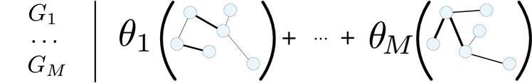
(a) Multigraph MT-MKL

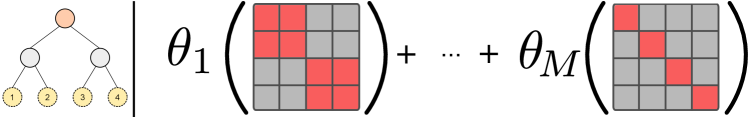
(b) Hierarchical MT-MKL

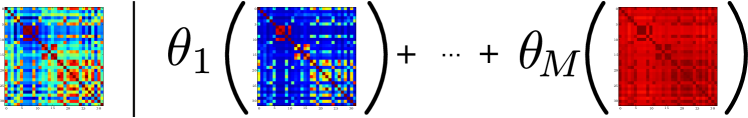
(c) Smooth MT-MKL

Figure 1: Learning additive transformations of task similarities: (a) Multigraph MT-MKL where one combines similarities from multiple independent graphs (which includes the approaches proposed in Widmer et al. (2010c); Jacob and Vert (2008)); (b) Hierarchical MT-MKL where one uses a tree to generate specific similarity matrices (as proposed in Widmer et al. (2010a, c); Görnitz et al. (2011); Widmer et al. (2012)); and (c) Smooth MT-MKL where one uses multiple transformations of an existing similarity matrix for linear combination.

2.6.1 Multi-graph MT-MKL

One of the most popular MTL approaches is graph-regularized MTL by Evgeniou and Pontil (2004). We have seen in Section 2.5.3, that such a graph is expressed as a adjacency matrix $A$ and may alternatively be expressed in terms of its graph Laplacian $L$. Our extension readily deals with multiple graphs encoding task similarity $A_{m}=(a_{mst})_{1\leq s,t\leq T}\in\mathbb{R}^{T\times T}$, which is of interest in cases where - as in Multiple kernel learning - we have access to alternative sources of task similarity and it is unclear which one is best suited. This concept gives rise to the multi-graph MTL regularizer

$$R(\boldsymbol{W})=\frac{1}{2}\operatorname*{tr}\left(\sum\nolimits_{m=1}^{M}W_{m}(I+L_{m})W_{m}^{\top}\right)\thinspace,$$

where $L_{m}$ denotes the graph Laplacian corresponding to $A_{m}$. As before, we learn a weighting of the given graphs, therefore determining which measures are best suited to maximize prediction accuracy.

2.6.2 Hierarchical MT-MKL

Recall that in task clustering, parameter vectors of tasks within the same cluster are coupled (Equation 13). The strength of that coupling, however, has be be chosen in advance and remains fixed throughout the learning procedure. We extend the formulation of task clustering by introducing a weighting $\theta_{m}$ to task cluster $m$ and tuning this weighting using our framework. We decompose $G$ over clusters and arrive at the following MTL regularizer

$$R(\boldsymbol{w}_{1},\ldots,\boldsymbol{w}_{T}) =\frac{1}{2}\left(\sum\nolimits_{m=1}^{M}\left\|\boldsymbol{w}_{m}\right\|^{2}+\sum\nolimits_{m=1}^{M}\theta_{m}\sum\nolimits_{s,t=1}^{T}G_{s,t}^{m}\langle\boldsymbol{w}_{s},\boldsymbol{w}_{t}\rangle\right)$$ (20)

$$=\frac{1}{2}\sum\nolimits_{m=1}^{M}\operatorname*{tr}\left(\theta_{m}W(I+G^{m})W^{\top}\right)\thinspace,$$ (21)

where $G^{m}$ is given by

$$G_{s,t}^{m}=\rho_{m}^{t}\delta_{st}-\frac{\rho_{m}^{s}\rho_{m}^{t}}{\rho+\sum_{r=1}^{T}\rho_{m}^{r}}.$$

Note that, if not all tasks belong to the same cluster, $G^{m}$ will not be invertible. Therefore, we need to express the mapping onto the dual of our general framework from Equation 10 in terms of the pseudo-inverse (see Equation 19) of $G_{m}$: $Q_{m}^{-1}=G_{m}^{\dagger}$.

An important special case of the above is given by a scenario where task relationships are described by a hierarchical structure $\mathcal{G}$ (see Figure 1(b)), such as a tree or a directed acyclic graph. Assuming hierarchical relations between tasks is particularly relevant to Computational Biology where often different tasks correspond to different organisms. In this context, we expect that the longer the common evolutionary history between two organisms, the more beneficial it is to share information between these organisms in a MTL setting. The tasks correspond to the leaves or terminal nodes and each inner node $n_{m}$ defines a cluster $m$, by grouping tasks of all terminal nodes that are descendants of the current node $n_{m}$. As before, task clusters $G$ can be used in the way discussed in the previous section.

2.6.3 Smooth hierarchical MT-MKL

Finally, we present a variant that may be regarded as a smooth version of the hierarchical MT-MKL approach presented above. Here, however, we require access to a given task similarity matrix, which is then subsequently transformed by squared exponentials with different length scales, for instance, $\mathbf{Q}^{(m)}_{st}=exp(A_{st}/\sigma_{m})$. We use MT-MKL to learn a weighting of the kernels associated with the different length scales, which corresponds to finding the right level in the hierarchy to trade off information between tasks. As an example, consider Figure 1(c), where we show the original task similarity matrix and the transformed matrices at different length scales.

3 Algorithms

In this section, we present efficient optimization algorithms to solve the primal and dual problems, i.e., Problems 1 and 2, respectively. We distinguish the cases of linear and non-linear kernel matrices. For non-linear kernels, we can simply use existing MKL implementations, while, for linear kernels, we develop a specifically tailored large-scale algorithm that allows us to train on problems with a large number of data points and dimensions, as demonstrated on several data sets. We can even employ this algorithm for non-linear kernels, if the kernel admits a sparse, efficiently computable feature representation. For example, this is the case for certain string kernels and polynomial kernels of degree 2 or 3. Our algorithms are embedded into the COFFIN framework (Sonnenburg and Franc, 2010) and integrated into the SHOGUN large-scale machine learning toolbox (Sonnenburg et al., 2010).

3.1 General Algorithms for Non-linear Kernels

A very convenient way to numerically solve the proposed framework is to simply exploit existing MKL implementations. To see this, recall from Section 2.4 that if we use the multi-task kernels $\tilde{k}_{1},\ldots,\tilde{k}_{M}$ as defined in (5) as the set of multiple kernels, the completely dualized MKL formulation (see Problem 3) is given by,

$$\inf_{{\boldsymbol{\theta}}\in\Theta_{p}}~{}\sup_{{\boldsymbol{\alpha}}\in{\mathbb{R}}^{n}:\sum_{i=1}^{n}\alpha_{i}y_{i}=0}~{}\thinspace-\frac{1}{2}\Bigg{\|}\Bigg{(}\sum_{i,j=1}^{n}\alpha_{i}\alpha_{j}y_{i}y_{j}\sum_{m=1}^{M}\theta_{m}\tilde{k}_{m}(x_{i},x_{j})\Bigg{)}_{1\leq m\leq M}\Bigg{\|}_{p^{*}}~{}-~{}C\thinspace{\mathfrak{L}}^{*}(-{\boldsymbol{\alpha}}/C)\thinspace.$$

An efficient optimization approach is by Vishwanathan et al. (2010), who optimize the completely dualized MKL formulation. This implementation comes along without a ${\boldsymbol{\theta}}$-step, but any of the $\alpha_{i}$-steps computations of the $\alpha_{i}$-steps are more costly as in the case of vanilla (MT-)SVMs.

Further, combining the partially dualized formulation in Problem 2 with the definition of multi-task kernels from (5), we arrive at an equivalent problem to (7), that is,

$$\inf_{{\boldsymbol{\theta}}\in\Theta_{p}}~{}\sup_{{\boldsymbol{\alpha}}\in{\mathbb{R}}^{n}}~{}\thinspace-\frac{1}{2}\sum_{i,j=1}^{n}\alpha_{i}\alpha_{j}y_{i}y_{j}\sum_{m=1}^{M}\tilde{k}_{m}(x_{i},x_{j})~{}-~{}C\thinspace{\mathfrak{L}}^{*}(-{\boldsymbol{\alpha}}/C)\thinspace,$$

which is exactly the optimization problem of $\ell_{p}$-norm multiple kernel learning as described in Kloft et al. (2011). We may thus build on existing research in the field of MKL and use one of the prevalent efficient implementations to solve $\ell_{p}$-norm MKL. Most of the $\ell_{p}$-norm MKL solvers are specifically tailored to the hinge loss. Proven implementations are, for example, the interleaved optimization method of Kloft et al. (2011), which is directly integrated into the SVMLight module (Joachims, 1999) of the SHOGUN toolbox such that the ${\boldsymbol{\theta}}$-step is performed after each decomposition step, i.e., after solving the small QP occurring in SVMLight, which allows very fast convergence (Sonnenburg et al., 2006).

For an overview of MKL algorithms and their implementations, see the survey paper by Gönen and Alpaydin (2011).

3.2 A Large-scale Algorithm for Linear or String Kernels and Beyond

For specific kernels such as linear kernels and string kernels—and, more generally, any kernel admitting an efficient feature space representation—, we can derive a specifically tailored large-scale algorithm. This requires considerably more work than the algorithm presented in the previous subsection.

3.2.1 Overview

From a top-level view, the upcoming algorithm underlies the core idea of alternating the following two steps:

1. the ${\boldsymbol{\theta}}$ step, where the kernel weights are improved

2. the $\boldsymbol{W}$ step, where the remaining primal variables are improved.

1:  input: data $x_{1},\ldots,x_{n}\in\mathcal{X}$ and labels  $y_{1},\ldots,y_{n}\in\{-1,1\}$ associated with tasks  $\tau(1),\ldots,\tau(n)\in\{1,\ldots,T\}$; feature vectors $\phi_{1}(x_{i}),\ldots,\phi_{M}(x_{i})$; task similarity matrices $Q_{1},\ldots,Q_{M}$; optimization precision $\varepsilon$

2:  initialize $\theta_{m}:=\sqrt[p]{1/M}$ for all $m=1,\ldots,M$, initialize $\boldsymbol{W}=\mathbf{0}$

3:  while optimality conditions are not satisfied within tolerance $\epsilon$ do

4:    $\boldsymbol{W}$ descent step: compute new $\boldsymbol{W}$ such that the obj. ${\mathfrak{R}}_{{\boldsymbol{\theta}}}(\boldsymbol{W})\thinspace+\thinspace C\thinspace{\mathfrak{L}}(\boldsymbol{W})$ decreases

5:              $\boldsymbol{W}:=\operatorname*{argmin}_{\widetilde{\boldsymbol{W}}}~{}{\mathfrak{R}}_{{\boldsymbol{\theta}}}(\widetilde{\boldsymbol{W}})\thinspace+\thinspace C\thinspace{\mathfrak{L}}(\widetilde{\boldsymbol{W}})$

6:    ${\boldsymbol{\theta}}$ step: compute minimizer ${\boldsymbol{\theta}}:=\operatorname*{argmin}_{\widetilde{{\boldsymbol{\theta}}}\in\Theta_{p}}~{}{\mathfrak{R}}_{\widetilde{{\boldsymbol{\theta}}}}(\boldsymbol{W})\thinspace+\thinspace C\thinspace{\mathfrak{L}}(\boldsymbol{W})$ according to (22)

7:  end while

8:  output: $\epsilon$-accurate optimal hypothesis $\boldsymbol{W}$ and kernel weights ${\boldsymbol{\theta}}$

Algorithm 1 (Blueprint of the large-scale optimization algorithm). The MKL module ($\theta$ step) is wrapped around the MTL module ($\boldsymbol{W}$ step).

These steps are illustrated in Algorithm Table 1. We observe from the table that the variables are split into the two sets $\left\{\theta_{m}|m=1,\ldots,M\right\}$ and $\left\{\boldsymbol{w}_{mt}|m=1,\ldots,M,t=1,\ldots,T\right\}$. The algorithm then alternatingly optimizes with respect to one or the other set until the optimality conditions are approximately satisfied. We will analyze convergence of this optimization scheme later in this section. Note that similar algorithms have been used in the context of the group lasso and multiple kernel learning by, for instance, Roth and Fischer (2008), Xu et al. (2010), and Kloft et al. (2011).

3.2.2 Solving the ${\boldsymbol{\theta}}$ Step

In this section, we discuss how to compute the update of the kernel weights ${\boldsymbol{\theta}}$ as carried out in Line 6 of Algorithm 1. Note that for fixed $\boldsymbol{W}\in{\mathcal{H}}$ it holds

$$\operatorname*{arginf}_{{\boldsymbol{\theta}}\in\Theta_{p}}\thinspace~{}{\mathfrak{R}}_{{\boldsymbol{\theta}}}(\boldsymbol{W})\thinspace+\thinspace C\thinspace{\mathfrak{L}}\big{(}A(\boldsymbol{W})\big{)}~{}\thinspace=~{}\thinspace\operatorname*{arginf}_{{\boldsymbol{\theta}}\in\Theta_{p}}\thinspace~{}{\mathfrak{R}}_{{\boldsymbol{\theta}}}(\boldsymbol{W})\thinspace,$$

where ${\mathfrak{R}}_{{\boldsymbol{\theta}}}(\boldsymbol{W})\thinspace=\thinspace\frac{1}{2}\sum_{m=1}^{M}\frac{\operatorname*{tr}(W_{m}Q_{m}W_{m})}{\theta_{m}}$. Furthermore, by Lagrangian duality,

$$\inf_{{\boldsymbol{\theta}}\in\Theta_{p}}~{}\frac{1}{2}\sum_{m=1}^{M}\frac{\operatorname*{tr}(W_{m}Q_{m}W_{m})}{\theta_{m}}\quad=\quad\max_{\lambda\geq 0}~{}~{}\inf_{{\boldsymbol{\theta}}\succeq\mathbf{0}}~{}\frac{1}{2}\sum_{m=1}^{M}\frac{\operatorname*{tr}(W_{m}Q_{m}W_{m})}{\theta_{m}}\thinspace+\thinspace\lambda\sum_{m=1}^{M}\theta_{m}^{p}$$

$$=~{}\inf_{{\boldsymbol{\theta}}\succeq\mathbf{0}}~{}\underbrace{\frac{1}{2}\sum_{m=1}^{M}\frac{\operatorname*{tr}(W_{m}Q_{m}W_{m})}{\theta_{m}}\thinspace+\thinspace\lambda^{*}\sum_{m=1}^{M}\theta_{m}^{p}}_{=:\psi({\boldsymbol{\theta}})}\thinspace,$$

where we denote the optimal $\lambda$ in the above maximization by $\lambda^{\star}$. The infimum is either attained at the boundary of the constraints or when $\nabla_{{\boldsymbol{\theta}}}\psi({\boldsymbol{\theta}})=0$, thus the optimal point ${\boldsymbol{\theta}}^{\star}$ satisfies $\theta_{m}^{\star}=\left(\operatorname*{tr}(W_{m}Q_{m}W_{m})/\lambda^{\star}\right)^{1/(p+1)}$ for any $m=1,\ldots,M$. Because ${\boldsymbol{\theta}}^{\star}\in\Theta_{p}$, i.e., $\left\|{\boldsymbol{\theta}}\right\|_{p}=1$, it follows $\lambda^{\star}=\left(\sum_{m=1}^{M}\operatorname*{tr}(W_{m}Q_{m}W_{m})^{p/(p+1)}\right)^{(p+1)/p}$, under the minimal assumption that $\boldsymbol{W}\neq\mathbf{0}$. Thus, because $\operatorname*{tr}(W_{m}Q_{m}W_{m})=\sum_{s,t=1}^{T}q_{mst}\left\langle\boldsymbol{w}_{ms},\boldsymbol{w}_{mt}\right\rangle$,

$$\forall m=1,\ldots,M:\quad\theta_{m}^{\star}=\frac{\sqrt[p+1]{\sum_{s,t=1}^{T}q_{mst}\left\langle\boldsymbol{w}_{ms},\boldsymbol{w}_{mt}\right\rangle}}{\left(\sum_{m=1}^{M}\sqrt[p+1]{\sum_{s,t=1}^{T}q_{mst}\left\langle\boldsymbol{w}_{ms},\boldsymbol{w}_{mt}\right\rangle}^{\thinspace p}\right)^{1/p}}\thinspace.$$ (22)

3.2.3 Solving the $\boldsymbol{W}$ Descent Step

To solve the $W$ step as carried out in Line 4 of Algorithm 1, we consider the kernel weights $\left\{\theta_{m}|m=1,\ldots,M\right\}$ as being fixed and optimize solely with respect to $\boldsymbol{W}$. In fact, we perform the $\boldsymbol{W}$ descent step in the dual, i.e., by optimizing the dual objective of Problem 2, i.e., solving

$$\sup_{{\boldsymbol{\alpha}}\in{\mathbb{R}}^{n}}~{}-{\mathfrak{R}}_{{\boldsymbol{\theta}}}^{*}(A^{*}({\boldsymbol{\alpha}}))\thinspace-\thinspace C\thinspace{\mathfrak{L}}^{*}(-({\boldsymbol{\alpha}})/C)\thinspace.$$

Although our framework is also valid for other loss functions, for the presentation of the algorithm, we make a specific choice of a proven loss function, that is, the hinge loss $l(a)=\max(0,1-a)$, so that by (8), the above task becomes

$$\sup_{{\boldsymbol{\alpha}}\in{\mathbb{R}}^{n}:\mathbf{0}\preceq{\boldsymbol{\alpha}}\preceq\bf{C}}~{}-{\mathfrak{R}}_{{\boldsymbol{\theta}}}^{*}(A^{*}({\boldsymbol{\alpha}}))\thinspace+\thinspace\sum_{i=1}^{n}\alpha_{i}\thinspace.$$ (23)

Our algorithm optimizes (23) by dual coordinate ascent, i.e., by optimizing the dual variables $\alpha_{i}$ one after another (i.e., only a single dual variable $\alpha_{i}$ is optimized at a time),

$$\sup_{d\in{\mathbb{R}}:\thinspace 0\leq\alpha_{i}+d\leq C}~{}~{}-{\mathfrak{R}}_{{\boldsymbol{\theta}}}^{*}(A^{*}({\boldsymbol{\alpha}}+d\boldsymbol{e}_{i}))\thinspace+\thinspace\sum_{i=1}^{n}\alpha_{i}+d\thinspace,$$

where we denote the unit vector of $i$th coordinate in ${\mathbb{R}}^{n}$ by $\boldsymbol{e}_{i}$. As we will see, this task can be performed analytically; however, performed purely in the dual involves computing a sum over all support vectors which is infeasible for large $n$. Our proposed algorithm is, instead, based on the application of the representer theorem carried out in Section 2.3: recall from (4) that, for all $m=1,\ldots,M$ and $t=1,\ldots,T$, it holds

$$\boldsymbol{w}_{mt}=\theta_{m}\sum_{i=1}^{n}q^{(-1)}_{m\tau(i)t}\alpha_{i}y_{i}\varphi_{m}(x_{i})\thinspace.$$

The core idea is to express the update of the $\alpha_{i}$ in the coordinate ascent procedure solely in terms of the vectors $\boldsymbol{w}_{mt}$. While optimizing the variables $\alpha_{i}$ one after another, we keep track of the changes in the vectors $\boldsymbol{w}_{mt}$. This procedure is reminiscent of the dual coordinate ascent method, but differs in the way the objective is computed. Of course, this implies that we need to manipulate feature vectors, which explains why our approach relies on efficient infrastructure of storing and computing feature vectors and their inner products. If the infrastructure is adequate so that computing inner products in the feature space is more efficient than computing a row of the kernel matrix, our algorithm will have a substantial gain.

Expressing the update of a single variable $\alpha_{i}$ in terms of the vectors $\boldsymbol{w}_{mt}$

As argued above, our aim is to express the (analytical) computation of

$$\sup_{d\in{\mathbb{R}}:\thinspace 0\leq\alpha_{i}+d\leq C}~{}~{}-{\mathfrak{R}}_{{\boldsymbol{\theta}}}^{*}(A^{*}({\boldsymbol{\alpha}}+d\boldsymbol{e}_{i}))\thinspace+\thinspace\sum_{i=1}^{n}\alpha_{i}+d\thinspace.$$

solely in terms of the vectors $\boldsymbol{w}_{mt}$. To start the derivation, note that, by (3),

$${\mathfrak{R}}_{{\boldsymbol{\theta}}}^{*}(A^{*}({\boldsymbol{\alpha}}+d\boldsymbol{e}_{i}))~{}=~{}\frac{1}{2}\sum_{m=1}^{M}\theta_{m}\left\|A^{*}({\boldsymbol{\alpha}}+d\boldsymbol{e}_{i})\right\|^{2}_{Q_{m}^{-1}}$$

with, by (6),

$$\left\|A^{*}({\boldsymbol{\alpha}}+d\boldsymbol{e}_{i})\right\|^{2}_{Q_{m}^{-1}}~{}=~{}\sum_{j,\tilde{j}=1}^{n}\alpha_{j}\alpha_{\tilde{j}}y_{j}y_{\tilde{j}}\tilde{k}_{m}(x_{j},x_{\tilde{j}})\thinspace+\thinspace 2dy_{i}\sum_{j=1}^{n}\alpha_{j}y_{j}\tilde{k}_{m}(x_{i},x_{j})\thinspace+\thinspace d^{2}k_{m}(x_{i},x_{i})\thinspace,$$

where

$$\tilde{k}_{m}(x_{i},x_{j})\thinspace=\thinspace q^{(-1)}_{m\tau(i)\tau(j)}k_{m}(x_{i},x_{j})$$

is the $m$th multi-task kernel as defined in (5). Thus,

$$\operatorname*{argsup}_{d\in{\mathbb{R}}:\thinspace 0\leq\alpha_{i}+d\leq C}~{}-{\mathfrak{R}}_{{\boldsymbol{\theta}}}^{*}(A^{*}({\boldsymbol{\alpha}}+d\boldsymbol{e}_{i}))\thinspace+\thinspace\sum_{i=1}^{n}\alpha_{i}+d$$

$$= \operatorname*{argsup}_{d\in{\mathbb{R}}:\thinspace 0\leq\alpha_{i}+d\leq C}~{}~{}d\thinspace-\thinspace dy_{i}\sum_{j=1}^{n}\alpha_{j}y_{j}\left(\sum\nolimits_{m=1}^{M}\theta_{m}\tilde{k}_{m}(x_{i},x_{j})\right)\thinspace-\thinspace\frac{1}{2}d^{2}\left(\sum\nolimits_{m=1}^{M}\theta_{m}\tilde{k}_{m}(x_{i},x_{i})\right)$$

$$= \operatorname*{argsup}_{d\in{\mathbb{R}}:\thinspace 0\leq\alpha_{i}+d\leq C}~{}~{}d\thinspace-\thinspace\underbrace{dy_{i}\left(\sum\nolimits_{m=1}^{M}\left\langle\boldsymbol{w}_{m\tau(i)},\varphi_{m}(x_{i})\right\rangle\right)\thinspace-\thinspace\frac{1}{2}d^{2}\left(\sum\nolimits_{m=1}^{M}\theta_{m}\tilde{k}_{m}(x_{i},x_{i})\right)}_{=:\psi(d)}\thinspace.$$

The optimum of $\psi(d)$ is either attained at the boundaries of the constraint $0\leq\alpha_{i}+d\leq C$ or when $\psi^{\prime}(d)=0$. Hence, the optimal $d^{\star}$ can be expressed analytically as

$$d^{\star}=\max\left(-\alpha_{i}\thinspace,~{}\min\left(C-\alpha_{i}\thinspace,\medspace\frac{1-y_{i}\sum\nolimits_{m=1}^{M}\theta_{m}\left\langle\boldsymbol{w}_{m\tau(i)},\varphi_{m}(x_{i})\right\rangle}{\sum\nolimits_{m=1}^{M}\theta_{m}\tilde{k}_{m}(x_{i},x_{i})}\right)\right)\thinspace.$$ (24)

Whenever we update an $\alpha_{i}$ according to

$$\alpha_{i}^{\rm new}:=\alpha_{i}^{\rm old}+d^{\star}$$

with $d$ computed as in (24), we need to also update the vectors $\boldsymbol{w}_{mt}$, $m=1,\ldots,M$, $t=1,\ldots,T$, according to

$$\boldsymbol{w}_{mt}^{\rm new}:=\boldsymbol{w}_{mt}^{\rm old}+d\theta_{m}q^{(-1)}_{m\tau(i)t}y_{i}\varphi_{m}(x_{i})\thinspace,$$ (25)

to be consistent with (4). Similarly, we need to update the vectors $\boldsymbol{w}_{mt}$ after each $\theta$ step according to

$$\boldsymbol{w}_{mt}^{\rm new}:=\left(\theta_{m}^{\rm new}/\theta_{m}^{\rm old}\right)\boldsymbol{w}_{mt}^{\rm old}\thinspace.$$ (26)

To avoid recurrences in the iterates, a ${\boldsymbol{\theta}}$-step should only be performed if the primal objective has decreased between subsequent ${\boldsymbol{\theta}}$-steps. Thus, after each ${\boldsymbol{\alpha}}$ epoch, the primal objective needs to be computed in terms of $\boldsymbol{W}$. As described above, the algorithm keeps $\boldsymbol{W}$ up to date when ${\boldsymbol{\alpha}}$ changes, which makes this task particular simple.

The resulting large-scale algorithm is summarized in Algorithm Table 2. Data and the labels are input to the algorithm as well as a sub-procedure for efficient computation of feature maps (cf. Section 3.2.4). Lines 2 and 3 initialize the optimization variables. In Line 4 the inverses of the task similarity matrices are pre-computed. Algorithm 2 iterates over Lines 7–16 until the stopping criterion falls under a pre-defined accuracy threshold $\varepsilon$. In Lines 7–11 the line search is computed for all dual variables. Lines 14 and 15 update the primal variables and kernel weights to be consistent with the representer theorem, only if the primal objective has decreased since the last ${\boldsymbol{\theta}}$-step. We stop Algorithm 2 when the relative change in the objective $o$ is less than $\epsilon$. Notice that we do not optimize the $W$ step to full precision, but instead alternate between one pass over the $\alpha_{i}$ and a ${\boldsymbol{\theta}}$ step.

1:  input: data $x_{1},\ldots,x_{n}\in\mathcal{X}$ and labels  $y_{1},\ldots,y_{n}\in\{-1,1\}$ associated with tasks  $\tau(1),\ldots,\tau(n)\in\{1,\ldots,T\}$; efficiently computable feature maps $\varphi_{1},\ldots,\varphi_{M}$; task similarity matrices $Q_{1},\ldots,Q_{M}$; optimization precision $\varepsilon$

2:  for all $i\in\{1,\ldots,n\}$ initialize $\alpha_{i}=0$

3:  for all $m\in\{1,\ldots,M\}$ and $t\in\{1,\ldots,T\}$, initialize $\boldsymbol{w}_{mt}$ according to (4)

4:  for all $m\in\{1,\ldots,M\}$, compute inverse $Q_{m}^{-1}=\big{(}q_{mst}^{(-1)}\big{)}_{1\leq s,t\leq T}$

5:  initialize primal objective $o=nC$

6:  while optimality conditions are not satisfied do

7:    for all $i\in\{1,\ldots,n\}$

8:      compute $d$ according to (24)

9:      update $\alpha_{i}:=\alpha_{i}+d$

10:      for all $m\in\{1,\ldots,M\}$ and $t\in\{1,\ldots,T\}$, update $\boldsymbol{w}_{mt}$ according to (25)

11:    end for

12:    store primal objective $o^{\rm old}=o$ and compute new primal objective $o$

13:    if primal objective has decreased, i.e., $o<o^{\rm old}$

14:      for all $m\in\{1,\ldots,M\}$, compute $\theta_{m}$ from $\boldsymbol{w}_{m1},\ldots,\boldsymbol{w}_{mT}$ according to (22)

15:      for all $m\in\{1,\ldots,M\}$ and $t\in\{1,\ldots,T\}$, update $\boldsymbol{w}_{mt}$ according to (26)

16:    end if

17:  end while

18:  output: $\epsilon$-accurate optimal hypothesis $\boldsymbol{W}=(\boldsymbol{w}_{mt})_{1\leq m\leq M,1\leq t\leq T}$ and kernel weights ${\boldsymbol{\theta}}=(\theta_{m})_{1\leq m\leq M}$

Algorithm 2 (Dual-coordinate-ascent-based MTL training algorithm). Generalization of the LibLinear training algorithm to multiple tasks and multiple linear kernels.

3.2.4 Details on the Implementation

We have implemented the optimization algorithms described in the previous section into the general framework of the SHOGUN machine learning toolbox (Sonnenburg et al., 2010). Besides the described implementations for binary classification, we also provide implementations for novelty detection and regression. Furthermore, the user may choose an optimization scheme, that is, decide whether one of the classic, non-linear MKL solvers shall be used (either the analytic optimization algorithm of Kloft et al. (2011), the cutting plane method of Sonnenburg et al. (2006), or the Newton algorithm by Kloft et al. (2009a)), or the novel implementation for efficiently computable feature maps. Our implementation can be downloaded from http://www.shogun-toolbox.org.

In the more conventional family of approaches, the wrapper algorithms, an optimization scheme on ${\boldsymbol{\theta}}$ wraps around a conventional SVM solver (for instance, LIBSVM and SVMLIGHT are integrated into SHOGUN) using a single multi-task kernel. Effectively, this results in alternatingly solving for ${\boldsymbol{\alpha}}$ and ${\boldsymbol{\theta}}$. For the ${\boldsymbol{\theta}}$-step, SHOGUN offers the three choices listed above. The second, much faster approach performs interleaved optimization and thus requires modification of the core SVM optimization algorithm. This is currently either integrated into the chunking-based SVRlight and SVMlight module. Lastly, the completely new optimization scheme as described in Algorithm Table 2 is implemented and connected with the module for computing the ${\boldsymbol{\theta}}$-step.

Note that the implementations for non-linear kernels come with the option of either pre-computing the kernel or computing the kernel on the fly for large-scale data sets. For truly large-scale MT-MKL, a linear or string kernel should be used. This is implemented as an internal interface the COFFIN module of SHOGUN (Sonnenburg and Franc, 2010).

3.3 Convergence Analysis

In this section, we establish convergence of Algorithm 1 under mild assumptions. To this end, we build on the existing theory of convergence of the block coordinate descent method. Classical results usually assume that the function to be optimized is strictly convex and continuously differentiable. This assertion is frequently violated in machine learning when, for instance, the hinge loss is employed. In contrast, we base our convergence analysis on the work of Tseng (2001) concerning the convergence of the block coordinate descent method. The following proposition is a direct consequence of Lemma 3.1 and Theorem 4.1 in Tseng (2001).

Proposition 4.

Let $f:\mathbb{R}^{d_{1}+\cdots+d_{R}}\rightarrow\mathbb{R}\cup\{\infty\}$ be a function. Put $d=d_{1}+\cdots+d_{R}$. Suppose that $f$ can be decomposed into $f({\boldsymbol{a}}_{1},\ldots,{\boldsymbol{a}}_{r})=f_{0}({\boldsymbol{a}}_{1},\ldots,{\boldsymbol{a}}_{r})+\sum_{r=1}^{R}f_{r}({\boldsymbol{a}}_{r})$ for some $f_{0}:\mathbb{R}^{d}\rightarrow\mathbb{R}\cup\{\infty\}$ and $f_{r}:\mathbb{R}^{d_{r}}\rightarrow\mathbb{R}\cup\{\infty\}$, $r=1,\ldots,R$. Initialize the block coordinate descent method by ${\boldsymbol{a}}^{0}=({\boldsymbol{a}}^{0}_{1},\ldots,{\boldsymbol{a}}^{0}_{R})$. Let $(r_{k})_{k\in\mathbb{N}}\subset\{1,\ldots,R\}$ be a sequence of coordinate blocks. Define the iterates ${\boldsymbol{a}}^{k}=({\boldsymbol{a}}^{k}_{1},\ldots,{\boldsymbol{a}}^{k}_{R})$, $k>0$, by

$${\boldsymbol{a}}_{r_{k}}^{k+1}\in\operatorname*{argmin}_{\mathfrak{A}\in\mathbb{R}^{d_{r_{k}}}}f\big{(}{\boldsymbol{a}}_{1}^{k+1},\cdots,{\boldsymbol{a}}_{r_{k}-1}^{k+1},\mathfrak{A},{\boldsymbol{a}}_{r_{k}+1}^{k},\cdots,{\boldsymbol{a}}_{R}^{k}\big{)}\thinspace,~{}~{}{\boldsymbol{a}}_{r}^{k+1}:={\boldsymbol{a}}_{r}^{k}\thinspace,~{}~{}r\neq r_{k}\thinspace,~{}~{}k\in\mathbb{N}_{0}\thinspace.$$ (27)

Assume that

• $f$ is convex and proper (i.e., $f\not\equiv\infty$)

• the sublevel set $\mathcal{A}^{0}:=\{{\boldsymbol{a}}\in\mathbb{R}^{d}:f({\boldsymbol{a}})\leq f({\boldsymbol{a}}^{0})\}$ is compact and $f$ is continuous on $\mathcal{A}^{0}$
  (assures existence of minimizer in (27))

• $\text{\rm dom}(f_{0}):=\{a\in\mathbb{R}^{d}:f_{0}({\boldsymbol{a}})<\infty\}$ is open and $f_{0}$ is Gâteaux differentiable (for instance, continuously differentiable) on $\text{\rm dom}(f_{0})$
  (yields regularity—i.e., any coordinate-wise minimum is a minimum of $f$)

• it exists a number $T\in\mathbb{N}$ so that, for each $k\in\mathbb{N}$ and $r\in\{1,\ldots,R\}$, there is $\tilde{k}\in\{k,\ldots,k+T\}$ with $r_{\tilde{k}}=r$ .
  (ensures that each coordinate block is optimized “sufficiently often”)

Then the minimizer in (27) exists and any cluster point of the sequence $({\boldsymbol{a}}^{k})_{k\in\mathbb{N}}$ minimizes $f$ over $\mathcal{A}$.

Corollary 5.

Assume that

• the data is represented by $\phi_{m}(x_{i})\in{\mathbb{R}}^{e_{m}}$, $i=1,\ldots,n$, $e_{m}<\infty$, $m=1,\ldots,M$.

• the loss function $l$ is convex, finite in 0, and continuous on its domain $\text{\rm dom}(l)$

• the task similarity matrices $Q_{1},\ldots,Q_{T}$ are positive definite

• any iterate ${\boldsymbol{\theta}}=(\theta_{1},\ldots,\theta_{M})$ traversed by Algorithm 1 has $\theta_{m}>0$, $m=1,\ldots,M$

• the exact search specified in Line 5 of Algorithm 1 is performed

Then Algorithm 1 is well-defined and any cluster point of the sequence traversed by the Algorithm 1 is a minimal point of Problem 1.

Proof.

The corollary is obtained by applying Proposition 4 to Problem 1, that is,

$$\inf_{\boldsymbol{W},\thinspace{\boldsymbol{\theta}}:~{}{\boldsymbol{\theta}}\in\Theta_{p}}~{}\frac{1}{2}\sum_{m=1}^{M}\frac{\|W_{m}\|^{2}_{Q_{m}}}{\theta_{m}}\thinspace+\thinspace C\sum_{i=1}^{n}l\bigg{(}y_{i}\sum_{m=1}^{M}\big{\langle}\boldsymbol{w}_{m\tau(i)},\varphi_{m}(x_{i})\big{\rangle}\bigg{)}\thinspace,$$ (28)

where $\Theta_{p}=\{{\boldsymbol{\theta}}\in\mathbb{R}^{M}:\theta_{m}\geq 0,m=1,\ldots,M,\left\|{\boldsymbol{\theta}}\right\|_{p}\leq 1\}$ and, by (B1), $\boldsymbol{W}\in\mathbb{R}^{eT}$, $e=e_{1}+\cdots+e_{M}$. Note that (28) can be written unconstrained as

$$\inf_{\boldsymbol{W},\thinspace{\boldsymbol{\theta}}}~{}f(\boldsymbol{W},{\boldsymbol{\theta}})\thinspace,\quad\text{\rm where}~{}~{}f(\boldsymbol{W},{\boldsymbol{\theta}})~{}:=~{}f_{0}(\boldsymbol{W},{\boldsymbol{\theta}})+f_{1}(\boldsymbol{W})+f_{2}({\boldsymbol{\theta}})\thinspace,$$ (29)

by putting

$$f_{0}(\boldsymbol{W},{\boldsymbol{\theta}})~{}:=~{}\frac{1}{2}\sum_{m=1}^{M}\frac{\|W_{m}\|^{2}_{Q_{m}}}{\theta_{m}}\thinspace+\thinspace I_{\{{\boldsymbol{\theta}}\succ\mathbf{0}\}}({\boldsymbol{\theta}})$$

as well as

$$f_{1}(\boldsymbol{W})~{}:=~{}C\sum_{i=1}^{n}l\bigg{(}y_{i}\sum_{m=1}^{M}\big{\langle}\boldsymbol{w}_{m\tau(i)},\varphi_{m}(x_{i})\big{\rangle}\bigg{)}\thinspace,\quad f_{2}({\boldsymbol{\theta}})~{}:=~{}I_{\{\left\|{\boldsymbol{\theta}}\right\|_{p}\leq 1\}}({\boldsymbol{\theta}})\thinspace,$$ (30)

where $I$ is the indicator function, $I_{S}(s)=0$ if $s\in S$ and $I_{S}(s)=\infty$ elsewise. Note that we use the shorthand ${\boldsymbol{\theta}}\succ\mathbf{0}$ for $\theta_{m}>0$, $m=1,\ldots,M$.

Assumption (B4) ensures that applying the block coordinate descent method to (28) and (29) problems yields precisely the sequence of iterates. Thus, in order to prove the corollary, it suffices to validate that (29) fulfills Assumptions (A1)–(A4) in Proposition 4.

Validity of (A1)   Recall that Algorithm 1 is initialized with $\boldsymbol{W}^{0}=\mathbf{0}$ and $\theta_{m}^{0}=\sqrt[p]{1/M}$, $m=1,\ldots,M$, so it holds

$$f(\boldsymbol{W}^{0},{\boldsymbol{\theta}}^{0})~{}=~{}\underbrace{f_{0}(\boldsymbol{W}^{0},{\boldsymbol{\theta}}^{0})}_{=0}~{}+\underbrace{f_{1}(\boldsymbol{W}^{0})}_{=Cn\thinspace l(0)}+~{}\underbrace{f_{2}({\boldsymbol{\theta}}^{0})}_{=0}~{}=~{}Cn\thinspace l(0)~{}<~{}\infty\thinspace,$$ (31)

hence $f\not\equiv\infty$, so $f$ is proper. Furthermore, $\text{\rm dom}(f_{0})=\{(\boldsymbol{W},{\boldsymbol{\theta}}):{\boldsymbol{\theta}}\succ\mathbf{0}\}$ is convex, and $f_{0}$ is convex on $\text{\rm dom}(f_{0})$, so $f_{0}$ is a convex function. By (B2), the loss function $l$ is convex, so $f_{1}$ is a convex function. The domain $\text{\rm dom}(f_{2})=\{{\boldsymbol{\theta}}:\left\|{\boldsymbol{\theta}}\right\|_{p}\leq 1\}$ is convex, and $f_{2}\equiv 0$ on its domain, so $f_{2}$ is a convex function. Thus the sum $f=f_{0}+f_{1}+f_{2}$ is a convex function, which shows (A1).

Validity of (A2)   Let $(\widetilde{\boldsymbol{W}},\widetilde{{\boldsymbol{\theta}}})\in\mathcal{A}^{0}:=\{(\boldsymbol{W},{\boldsymbol{\theta}}):f(\boldsymbol{W},{\boldsymbol{\theta}})\leq f(\boldsymbol{W}^{0},{\boldsymbol{\theta}}^{0})\}$. We have $f_{0},f_{1},f_{2}\geq 0$, so, for all $m=1,\ldots,M$,

$$\begin{split}\frac{\|\widetilde{W}_{m}\|_{Q_{m}}}{2\theta_{m}}&~{}\leq~{}f_{0}(\widetilde{\boldsymbol{W}},\widetilde{{\boldsymbol{\theta}}})~{}\leq~{}f_{0}(\widetilde{\boldsymbol{W}},\widetilde{{\boldsymbol{\theta}}})+\underbrace{f_{1}(\widetilde{\boldsymbol{W}})}_{\geq 0}+\underbrace{f_{2}(\widetilde{{\boldsymbol{\theta}}})}_{\geq 0}\thinspace\stackrel{{\scriptstyle\rm by\thinspace\eqref{eq:prob2}}}{{=}}\thinspace f(\widetilde{\boldsymbol{W}},\widetilde{{\boldsymbol{\theta}}})\\ &~{}\leq~{}f(\boldsymbol{W}^{0},{\boldsymbol{\theta}}^{0})\thinspace\stackrel{{\scriptstyle\rm by\thinspace\eqref{eq:finite}}}{{\leq}}\thinspace Cn\thinspace l(0)\thinspace,\end{split}$$ (32)

which implies $\|\widetilde{W}_{m}\|^{2}_{Q_{m}}\leq 2\theta_{m}Cn\thinspace l(0)$. Similar, because $f_{0}\geq 0$, we have $f_{2}(\widetilde{\boldsymbol{W}},\widetilde{{\boldsymbol{\theta}}})\leq Cn\thinspace l(0)<\infty$, which, by (30), implies $\|\widetilde{{\boldsymbol{\theta}}}\|_{p}\leq 1$ and thus $\widetilde{\theta}_{m}\leq 1$, $m=1,\ldots,M$. Hence, by (32), $\|\widetilde{W}_{m}\|^{2}_{Q_{m}}\leq\thinspace 2Cn\thinspace l(0)$, $m=1,\ldots,M$. Because $Q_{1},\ldots,Q_{M}$ are positive definite, $\nu:=\min_{m=1,\ldots,M}\operatorname*{tr}(Q_{m})>0$. Thus, for any $m=1,\ldots,M$,

$$\|\widetilde{W}_{m}\|^{2} = \operatorname*{tr}(\widetilde{W}_{m}^{*}\widetilde{W}_{m})~{}=~{}\operatorname*{tr}(\widetilde{W}_{m}^{*}\widetilde{W}_{m})\operatorname*{tr}(Q_{m})/\operatorname*{tr}(Q_{m})~{}\leq~{}\operatorname*{tr}(\widetilde{W}_{m}^{*}W_{m}Q_{m})/\operatorname*{tr}(Q_{m})$$

$$\leq \nu^{-1}\thinspace\operatorname*{tr}(\widetilde{W}_{m}^{*}\widetilde{W}_{m}Q_{m})~{}=~{}\nu^{-1}\thinspace\operatorname*{tr}(\widetilde{W}_{m}Q_{m}\widetilde{W}_{m}^{*})~{}=~{}\nu^{-1}\thinspace\|\widetilde{W}_{m}\|_{Q_{m}}^{2}~{}\leq~{}2\nu^{-1}Cn\thinspace l(0)\thinspace.$$

Thus

$$\|(\widetilde{\boldsymbol{W}},\widetilde{{\boldsymbol{\theta}}})\|^{2}~{}=~{}\|\widetilde{\boldsymbol{W}}\|^{2}+\|\widetilde{{\boldsymbol{\theta}}}\|^{2}~{}\leq~{}2\nu^{-1}CMn\thinspace l(0)+M~{}<~{}\infty\thinspace.$$

Thus $\sup_{(\widetilde{W},\widetilde{{\boldsymbol{\theta}}})\in\mathcal{A}^{0}}\|(\widetilde{W},\widetilde{{\boldsymbol{\theta}}})\|<\infty$, which shows that $\mathcal{A}^{0}$ is bounded. Furthermore, $\mathcal{A}^{0}\subset\text{\rm dom}(f)=\text{\rm dom}(f_{0})\cap\text{\rm dom}(f_{1})\cap\text{\rm dom}(f_{2})$ and $f_{0},f_{1},f_{2}$ are continuous on their respective domains. Thus $f$ is continuous on $\text{\rm dom}(f)$ and thus also on its subset $\mathcal{A}^{0}$. It holds $\mathcal{A}^{0}=f^{-1}\big{(}]-\infty,f(\boldsymbol{W}^{0},{\boldsymbol{\theta}}^{0})]\big{)}$, i.e., $\mathcal{A}^{0}$ is the preimage of closed set under a continuous function; thus $\mathcal{A}^{0}$ is closed. Any closed and bounded subset of $\mathbb{R}^{d}$ is compact. Thus $\mathcal{A}^{0}$ is compact, which was to show.

Validity of (A3) and (A4)   Clearly, $\text{\rm dom}(f_{0})=\{(\boldsymbol{W},{\boldsymbol{\theta}}):{\boldsymbol{\theta}}\succ\mathbf{0}\}$ is open and $f_{0}$ is continuously differentiable on $\text{\rm dom}(f_{0})$. Thus it is Gâteaux differentiable on $\text{\rm dom}(f_{0})$. Finally, assumption (A4) is trivially fulfilled as Algorithm 1 employs a simple alternating rule for traversing the blocks of coordinates.

In summary, Proposition 4 can thus be applied to Problem 1, which yields the claim of the corollary. ∎

Remark 6.

In this paper, we experiment on finite-dimensional string kernels, so Assumption (B1) is naturally fulfilled. Note that, more generally, $\phi(x_{i})\in{\mathbb{R}}^{d_{m}}$ for all $i=1,\ldots,n$, $m=1,\ldots,M$, can be enforced also for infinite-dimensional kernels, as, for any finite sample $x_{1},\ldots,x_{n}$, there exists a $n$-dimensional feature representation of the sample that can be explicitly computed in terms of the empirical kernel map (Schölkopf et al., 1999).

4 Applications

We demonstrate the performance of different facets of our framework with several experiments ranging from well-controlled toy data to a large scale experiment on a highly relevant genomes data set, where we combine data from a diverse set of organisms using multitask learning. We start with a review of our prior experimental work based on algorithms that are closely related to the ones described in this work.

4.1 Previous work

The theoretical framework presented in this paper is a generalization of the methods successfully used in our previous work. Special cases of the above framework were investigated in the context of genomic signal prediction (Schweikert et al., 2008; Widmer et al., 2010a), sequence segmentation with structured output learning (Görnitz et al., 2011), computational immunology (Widmer et al., 2010b, c; Toussaint et al., 2010) and problems from biological imaging (Lou et al., 2012; Widmer et al., 2014; Lou et al., 2014). Further, we have investigated an efficient algorithm to solve special cases of our method on a large number of machine learning data sets in Widmer et al. (2012). We have previously summarized some of our earlier work in (Widmer and Rätsch, 2012; Widmer et al., 2013a, b).

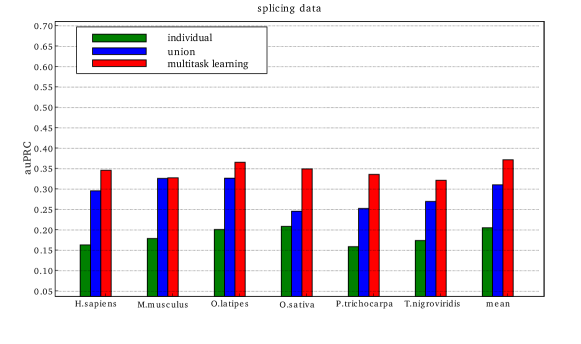
Figure 2: Results from multitask learning on several organisms. Shown is a subset of the results reported in Widmer et al. (2010a), where we combined splice site data from $15$ organisms. We compared a multitask learning approach to baseline methods individual (each task is learned independently) and union (all data is simply pooled). As for multitask learning, we used only a single, fix similarity measure, which we inferred from the evolutionary history of the organisms at hand. These and other results in Schweikert et al. (2008); Widmer et al. (2010a); Görnitz et al. (2011); Widmer et al. (2010b, c); Toussaint et al. (2010); Lou et al. (2012); Widmer et al. (2014); Lou et al. (2014) illustrate the power multitask learning in related tasks in computational biology.

An example of earlier results from Widmer et al. (2010a) is given in Figure 2. It illustrates an application of the MTL algorithm to a case where we have multiple datasets associated with 15 organisms. Their evolutionary relationship is assumed to be known and is used for informing task relatedness in the algorithm that is described in Section 2.5.3 and Widmer et al. (2010a). This experiment exemplifies the successful application of MTL to applications in computational biology for the joint-analysis of multiple related problems.

In the two experiments that will be described in the sequel, we will go beyond our previous work by investigating our framework in its full generality.

4.2 Experiments on Biologically Motivated Controlled Data

In this section, we evaluate Hierarchical MT-MKL as described in Section 2.6.2 on an artificial data set motivated by biological evolution. At the core of this example is the binary classification of examples generated from two $100$-dimensional isotropic Gaussian distributions with a standard deviation of $\sigma=20$. The difference of the mean vectors $\mu_{pos}$ and $\mu_{neg}$ is captured by a difference vector $\mu_{d}$. We set $\mu_{pos}=0.5\mu_{d}$ and $\mu_{neg}=-0.5\mu_{d}$. To turn this into a MTL setting, we start with a single $\mu_{d}=(1,\dots,1)^{T}$ and apply mutations to it. These mutations correspond to flipping the sign of $m$ dimensions in $\mu_{d}$, where $m=5$. Inspired by biological evolution, mutations are then applied in a hierarchical fashion according to a binary tree of depth $4$ (corresponding to $2^{4}=32$ leaves). Starting at the root node, we apply subsequent mutations to the $\mu_{d}$ at the inner nodes of the hierarchy and work down the tree until each leaf carries its own $\mu_{d}$. We sample $10$ training points and $1,000$ test points for each class and for each of the $32$ tasks. The similarity between the $\mu_{d}$ at the leaves is computed by taking the dot product between all pairs and is shown in Figure 3(a). Clearly, this information is valuable when deciding which tasks (corresponding to leaves in this context) should be coupled and will be referred to as the true task similarity matrix in the following. We use Hierarchical MT-MKL as described in Section 2.6.2 by creating adjacency matrices for each inner node and subsequently learning a weighting using MT-MKL.

We compare MT-MKL with $p={1,2,3}$ to the following baseline methods: Union that combines data from all tasks into a single group, Individual that treats each task separately and Vanilla MTL that uses MTL with the same weight for all matrices. We report the mean (averaged over tasks) ROC curve for each of the above methods in Figure 3(b).

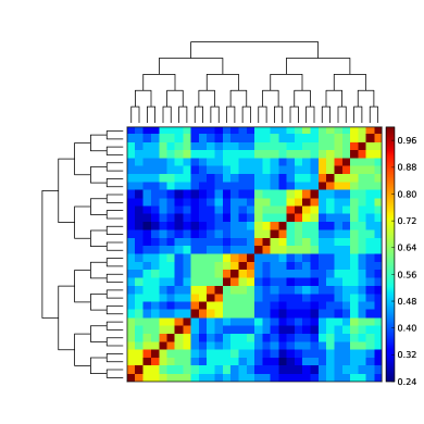
(a) True Task similarity matrix (see main text)

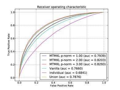
(b) Performance of Hierarchical MT-MKL vs. Baseline methods

Figure 3: Illustration of Hierarchical MT-MKL on an artificial dataset: In 3(a), we show the similarity matrix between all $32$ tasks as generated by a biologically inspired scheme, where generating parameters are mutated according to a given tree structure (see main text for details). Comparison of MT-MKL to baselines Vanilla MTL, Union, Individual is shown in 3(b), where ROC curves are averaged over the $32$ tasks for each method. MT-MKL with $p=2$ and $p=3$ perform best for this task.

From Figure 3(b) we observe that the baseline Individual performs worst by a large margin, suggesting that combining information from several tasks is clearly beneficial for this data set. Next, we observe that a simple way of combining tasks (i.e., Union) already considerably improves performance. Furthermore, we observe that learning weights of hierarchically inferred task grouping in fact improves performance compared to Vanilla for non-sparse MT-MKL (i.e., $p=2,3$). Of all methods, non-sparse MT-MKL is most accurate for all recall values.

4.3 Genomic Signal - Transcription Start Site (TSS) Prediction

In this experiment, we consider an application from genome sequence analysis. The goal is to accurately identify the genomic signal called transcription start site (TSS) based on the surrounding genomic sequence. TSS is the genomic location where transcription, the process whereby the RNA copies are made from regions of the genome, is initiated at the genome sequences. We have obtained genomic data from ENSEMBL (Hubbard et al., 2002), a community resource that brings together genomic sequences and their annotations. From this, we compiled a data set for nine organisms (E. caballus, C. briggsae, M. musculus, C. elegans, D. rerio, D. simulans, V. vinifera, A. thaliana, and H. sapiens), where we took annotated instances of transcription starts as positive examples and sequences around randomly selected positions in the genome as background. We use our framework to jointly learn models for different organisms, treating different organisms as different tasks.

Task similarity

To generate an initial task similarity matrix, we extracted the phylogenetic similarity between different organisms based on their genomic sequences. In particular, we computed the Hamming distance between well-conserved 16S ribosomal RNA regions (i.e., stretches of genomic sequence with low degree of change during evolution) between different classes of organisms (Isenbarger et al., 2008). Subsequently, we either used this similarity directly in our multitask learning algorithms (MTL) or attempted to refine it further using MT-MKL. To create a set of task similarities to be weighted by MT-MKL, we applied exponential transformations to the base task similarity at different length-scales ($\sigma=\{0.1,7.55,15.0\}$; see Section 2.6.3).

Experimental Setup and Results

We have collected 4,000 TSS signal sequences for each organism, which includes 1,000 positive and 3,000 negative label sequences for training and testing. Both ends of the TSS signal label sequence consist of $1,200$ flanking nucleotides. On this data set, we evaluated the two baseline methods, MTL and MT-MKL. In the used evaluation scheme, we split the data in training set, validation set and testing set for each organism. We use ten splits. The best regularization constant is selected on the validation split for each organism. In Figure 4 we report the average area under the ROC curve (AUC) over the ten test sets, for each of which the best regularization parameter was chosen on a separate evaluation set.

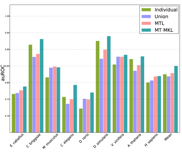
Figure 4: Average AUC achieved by the proposed MT-MKL as well as the baseline methods, on the gene-start dataset (TSS). MT-MKL improves the mean accuracy considerably. In addition, the accuracy of MT-MKL is best in eight out of the nine organisms.

From Figure 4, we observe that four out of nine organisms the single-task SVM (individual) outperforms the SVM that is trained on training instances from all organisms pooled (union). From which we conclude that the learning tasks are substantially dissimilar. On the other hand, we observe that for some organisms (M. musculus, D. rerio, V. vinifera, and H. sapiens), there is an improvement by union over individual, which indicates that these tasks are more similar than the remaining tasks. This is an indicator that MTL may be beneficial for this data. See also discussion in Widmer et al. (2013b). Indeed, MTL improves (at least marginally) over Union and Individual in seven and five out of nine organisms, respectively. But it is surpassed by Individual for three organisms (A. thaliana, C. briggsae, C. elegans, and D. simulans). While the overall performance of of MTL is slightly better than Union and Individual, the differences are minor which we attribute a possibly suboptimally chosen task similarity matrix. (In fact, practically speaking, we find that selecting a good task similarity matrix is the most difficult aspect of Multitask learning.)

The proposed MT-MKL on the other hand, improves over individual on eight out of nine organisms (and is not much worse on the nineth task). It improves over MTL by close to $5\%$ AUC for some organisms. On average, it performs about $2.5\%$ better than any other considered algorithm. MT-MKL achieves this by refining task similarities and thus is able to improve classification performance.

In summary, we are able to demonstrate that multitask learning and MT-MKL strategies are beneficial when combining information from several organisms and we believe that this setting has potential for tackling future prediction problems in computational biology, and potentially also to other application domains of multitask and multiple kernel learning such as computer vision (Lou et al., 2012; Kloft et al., 2009b; Binder et al., 2012; Widmer et al., 2014; Lou et al., 2014) and computer security (Kloft et al., 2008a; Kloft and Laskov, 2012; Görnitz et al., 2013).

5 Conclusion

We presented a general regularization-based framework for Multi-task learning (MTL), in which the similarity between tasks can be learned or refined using $\ell_{p}$-norm Multiple Kernel learning (MKL). Based on this very general formulation (including a general loss function), we derived the corresponding dual formulation using Fenchel duality applied to Hermitian matrices. We showed that numerous established MTL methods can be derived as special cases from both, the primal and dual of our formulation. Furthermore, we derived an efficient dual-coordinate descend optimization strategy for the hinge-loss variant of our formulation and provide convergence bounds for our algorithm. Combined with our efficient integration into the SHOGUN toolbox using the COFFIN feature hashing framework, the approach could be used to process a large number of training points. The solver can also be used to solve the vanilla $\ell_{p}$-norm MKL problem in the primal very efficiently, and potentially extended to more recent MKL approaches (Cortes et al., 2013). Our solvers including all discussed special cases are made available as open-source software as part of the SHOGUN machine learning toolbox.

In the experimental part of this paper, we analyzed our algorithm in terms of predictive performance and ability to reconstruct task relationships on toy data, as well as on problems from computational biology. This includes a study at the intersection of multitask learning and genomics, where we analyzed $9$ organisms jointly. In summary, we were able to demonstrate that the proposed learning algorithm can outperform baseline methods by combining information from several organisms.

In the future we would investigate the theoretical foundations of the approach (a good starting point to this end is the work by Kloft and Blanchard (2011, 2012)), extensions to structured output prediction (Görnitz et al., 2011), and to apply the method to further problems from computational biology and the biomedical domain. These settings have great potential; for instance, a Bayesian adaption of our approach was very recently shown to be the leading model in an international comparison of $44$ drug prediction methods for breast cancer (Costello et al., 2014).

Acknowledgements

We thank thank Bernhard Schölkopf, Gabriele Schweikert, Alexander Zien and Sören Sonnenburg for early contributions and helpful discussions and Klaus-Robert Müller and Mehryar Mohri for helpful discussions. This work was supported by the German Research Foundation (DFG) under MU 987/6-1 and RA 1894/1-1 as well as by the European Community’s 7th Framework Programme under the PASCAL2 Network of Excellence (ICT-216886). Marius Kloft acknowledges support by the German Research Foundation through the grants KL 2698/1-1 and 2698/2-1. Gunnar Rätsch acknowledges additional support from the Sloan Kettering Institute.

Appendix A Fenchel Duality in Hilbert Spaces

In this section, we review Fenchel duality theory for convex functions over real Hilbert spaces. The results presented in this appendix are taken from Chapters 15 and 19 in Bauschke and Combettes (2011). For complementary reading, we refer to the excellent introduction of Bauschke and Lucet (2012). Fenchel duality for machine learning has also been discussed in Rifkin and Lippert (2007) assuming Euclidean spaces. We start the presentation with the definition of the convex conjugate function.

Definition 7 (Convex conjugate).

Let ${\mathcal{H}}$ be a real Hilbert space and let $g:{\mathcal{H}}\rightarrow{\mathbb{R}}\cup\{\infty\}$ be a convex function. We assume in the whole section that $g$ is proper, that is, $\{\boldsymbol{w}\in{\mathcal{H}}\thinspace|\thinspace g(\boldsymbol{w})\in{\mathbb{R}}\}\neq\emptyset$. Then the convex conjugate $g^{*}:{\mathcal{H}}\rightarrow{\mathbb{R}}\cup\{\infty\}$ is defined by $g^{*}(\boldsymbol{w})=\sup_{\boldsymbol{v}\in{\mathcal{H}}}\langle\boldsymbol{v},\boldsymbol{w}\rangle-g(\boldsymbol{v})$.

As the convex conjugate is a supremum over affine functions, it is convex and lower semi-continuous. We have the beautiful duality

$$g=g^{**}\thinspace\Leftrightarrow\thinspace\begin{cases}g\text{ is convex and}\\ \text{lower semi-continuous}\thinspace.\end{cases}$$

This indicates that the “right domain” to study conjugate functions is the set of convex, lower semi-continuous, and proper (“ccp”) functions. In order to present the main result of this appendix, we need the following standard result from operator theory.

Proposition 8 (Definition and uniqueness of the adjoint map).

Let ${\mathcal{H}}$ be a real Hilbert space and let $A:{\mathcal{H}}\rightarrow\widetilde{{\mathcal{H}}}$ be a continuous linear map. Then there exists a unique continuous linear map $A^{*}:\widetilde{{\mathcal{H}}}\rightarrow{\mathcal{H}}$ with $\langle A(\boldsymbol{w}),{\boldsymbol{\alpha}}\rangle=\langle\boldsymbol{w},A^{*}{\boldsymbol{\alpha}}\rangle$, which is called adjoint map of $A$.

For example, in the Euclidean case, we have ${\mathcal{H}}={\mathbb{R}}^{m}$, $\widetilde{{\mathcal{H}}}={\mathbb{R}}^{n}$, and $A\in\mathbb{{\mathbb{R}}}^{m\times n}$ so that simply the transpose $A^{*}=A^{\top}\in\mathbb{{\mathbb{R}}}^{n\times m}$. We now present the main result of this appendix, which is known as Fenchel’s duality theorem:

Theorem 9 (Fenchel’s duality theorem).

Let ${\mathcal{H}},\widetilde{{\mathcal{H}}}$ be real Hilbert spaces and let $g:{\mathcal{H}}\rightarrow{\mathbb{R}}\cup\left\{\infty\right\}$ and $h:\widetilde{{\mathcal{H}}}\rightarrow{\mathbb{R}}\cup\left\{\infty\right\}$ be ccp. Let $A:{\mathcal{H}}\rightarrow\widetilde{{\mathcal{H}}}$ be a continuous linear map. Then the primal and dual problems,

$$p^{*}=\inf_{\boldsymbol{w}\in{\mathcal{H}}}~{}g(\boldsymbol{w})+h(A(\boldsymbol{w}))$$

$$d^{*}=\thinspace\sup_{{\boldsymbol{\alpha}}\in\widetilde{{\mathcal{H}}}}\thinspace-g^{*}(A^{*}({\boldsymbol{\alpha}}))-h^{*}(-{\boldsymbol{\alpha}})\thinspace,$$

satisfy weak duality (i.e., $d^{*}\leq p^{*}$). Assume, furthermore, that $A(\textrm{dom}(g))\cap\textrm{cont}(h)\neq\emptyset$, where $\text{\rm dom}(f):=\{\boldsymbol{w}\in{\mathcal{H}}:g(\boldsymbol{w})<\infty\}$ and $\text{\rm cont(h)}:=\{{\boldsymbol{\alpha}}\in\widetilde{{\mathcal{H}}}:h~{}\textrm{continuous~{}in}~{}{\boldsymbol{\alpha}}\}$. Then we even have strong duality (i.e., $d^{*}=p^{*}$) and any optimal solution $(\boldsymbol{w}^{\star},{\boldsymbol{\alpha}}^{\star})$ satisfies

$$\boldsymbol{w}^{\star}=\nabla g^{*}(A^{*}({\boldsymbol{\alpha}}^{\star}))\thinspace,$$

if $g^{*}\circ A^{*}$ is (Gâteaux) differentiable in ${\boldsymbol{\alpha}}^{\star}$.

When applying Fenchel duality theory, we frequently need to compute the convex conjugates of certain functions. To this end, the following computation rules are helpful.

Proposition 10.

The following computation rules hold for the convex conjugate:

1. Let $g:{\mathcal{H}}\rightarrow{\mathbb{R}}\cup\left\{\infty\right\}$ be a proper convex function on a real Hilbert space ${\mathcal{H}}$. Then, for any $\lambda>0$ and $\boldsymbol{w}\in{\mathcal{H}}$, we have $(\lambda g)^{*}(\boldsymbol{w})=\lambda h^{*}(\boldsymbol{w}/\lambda)$.

2. Furthermore, assume that ${\mathcal{H}}={\mathcal{H}}_{1}\bigoplus{\mathcal{H}}_{2}$ and $g(\boldsymbol{w})=g_{1}(\boldsymbol{w}_{1})+g_{2}(\boldsymbol{w}_{2})$, where $g_{1}:{\mathcal{H}}_{1}\rightarrow{\mathbb{R}}\cup\left\{\infty\right\}$ and $g_{2}:{\mathcal{H}}_{2}\rightarrow{\mathbb{R}}\cup\left\{\infty\right\}$, are proper convex functions on Hilbert spaces ${\mathcal{H}}_{1}$ and ${\mathcal{H}}_{2}$, respectively. Then, for any $\boldsymbol{w}=(\boldsymbol{w}_{1},\boldsymbol{w}_{2})\in{\mathcal{H}}_{1}\bigoplus{\mathcal{H}}_{2}$, we have $g^{*}(\boldsymbol{w})=g_{1}^{*}(\boldsymbol{w}_{1})+g^{*}_{2}(\boldsymbol{w}_{2})$.

Appendix B Conjugate of the Logistic Loss

The following lemma gives the convex conjugate of the logistic loss.

Lemma 11 (Conjugate of Logistic Loss).

The conjugate of the logistic loss, defined as $l(a)=\log(1+\exp(-a)$, is given by

$$l^{*}(a)=-t\log(-a)+(1+a)\log(1+a)\thinspace.$$

Proof.

By definition of the conjugate,

$$l^{*}(a)~{}=~{}\sup_{b\in{\mathbb{R}}}~{}\underbrace{ab\thinspace-\thinspace\log(1+\exp(-b))}_{=:\psi(b)}\thinspace.$$

Note that the problem is unbounded for $a<-1$ and $a>0$. For $a\in]-1,0[$, the supremum is attained when $\psi^{\prime}(b)=0$, which translates into $b=-\log(-a/(1+a))$ and $1+\exp(-b)=1/(1+a)$. Thus

$$l^{*}(a)\thinspace=\thinspace-a\log(-a/(1+a))-\log(1/(1+a))\thinspace=\thinspace-a\log(-a)+(1+a)\log(1+a)\thinspace,$$

which was to show ∎

References

- Agarwal et al. (2010) A. Agarwal, H. Daumé III, and S. Gerber. Learning Multiple Tasks using Manifold Regularization. In Advances in Neural Information Processing Systems 23, 2010.
- Ahn and Brewer (1993) W.-K. Ahn and W. F. Brewer. Psychological studies of explanation—based learning. In Investigating explanation-based learning, pages 295–316. Springer, 1993.
- Ando and Zhang (2005) R. K. Ando and T. Zhang. A Framework for Learning Predictive Structures from Multiple Tasks and Unlabeled Data. Journal of Machine Learning Research, 6(6):1817–1853, 2005. ISSN 15324435.
- Argyriou et al. (2007) A. Argyriou, T. Evgeniou, and M. Pontil. Multi-task feature learning. NIPS 2007, 2007.
- Argyriou et al. (2008a) A. Argyriou, T. Evgeniou, and M. Pontil. Convex multi-task feature learning. Machine Learning, 73(3):243–272, 2008a. ISSN 0885-6125.
- Argyriou et al. (2008b) A. Argyriou, C. Micchelli, M. Pontil, and Y. Ying. A spectral regularization framework for multi-task structure learning. Advances in Neural Information Processing Systems, 20:25–32, 2008b.
- Argyriou et al. (2009) A. Argyriou, C. Micchelli, and M. Pontil. When is there a representer theorem? Vector versus matrix regularizers. The Journal of Machine Learning Research, 10:2507–2529, 2009. ISSN 1532-4435.
- Bauschke and Lucet (2012) H. Bauschke and Y. Lucet. What is a fenchel conjugate? Notices of the AMS, 59:44–46, 2012.
- Bauschke and Combettes (2011) H. H. Bauschke and P. L. Combettes. Convex analysis and monotone operator theory in Hilbert spaces. CMS Books in mathematics. Springer, New York, 2011. ISBN 1441994661.
- Baxter (2000) J. Baxter. A model of inductive bias learning. Journal of Artificial Intelligence Research, 12(1):149–198, Feb. 2000. ISSN 1076-9757.
- Binder et al. (2012) A. Binder, S. Nakajima, M. Kloft, C. Müller, W. Samek, U. Brefeld, K.-R. Müller, and M. Kawanabe. Insights from classifying visual concepts with multiple kernel learning. PloS one, 7(8):e38897, 2012.
- Caruana (1993) R. Caruana. Multitask learning: A knowledge-based source of inductive bias. In ICML, pages 41–48. Morgan Kaufmann, 1993. ISBN 1-55860-307-7.
- Caruana (1997) R. Caruana. Multitask Learning. Machine Learning, 28(1):41 – 75, 1997. ISSN 08856125. doi: 10.1023/A:1007379606734.
- Chen et al. (2009) J. Chen, L. Tang, J. Liu, and J. Ye. A convex formulation for learning shared structures from multiple tasks. In Proceedings of the 26th Annual International Conference on Machine Learning - ICML ’09, pages 1–8, New York, New York, USA, June 2009. ACM Press. ISBN 9781605585161. doi: 10.1145/1553374.1553392.
- Cortes et al. (2013) C. Cortes, M. Kloft, and M. Mohri. Learning kernels using local rademacher complexity. In Advances in Neural Information Processing Systems, pages 2760–2768, 2013.
- Costello et al. (2014) J. C. Costello, L. M. Heiser, E. Georgii, M. Gönen, M. P. Menden, N. J. Wang, M. Bansal, P. Hintsanen, S. A. Khan, J.-P. Mpindi, et al. A community effort to assess and improve drug sensitivity prediction algorithms. Nature Biotechnology, 2014. doi:10.1038/nbt.2877, to appear.
- Daumé (2007) H. Daumé. Frustratingly easy domain adaptation. In Annual meeting-association for computational linguistics, volume 45, page 256, 2007.
- Evgeniou and Pontil (2004) T. Evgeniou and M. Pontil. Regularized multi-task learning. In International Conference on Knowledge Discovery and Data Mining, pages 109–117, 2004.
- Evgeniou et al. (2005) T. Evgeniou, C. Micchelli, and M. Pontil. Learning multiple tasks with kernel methods. Journal of Machine Learning Research, 6(1):615–637, 2005. ISSN 1532-4435.
- Gönen and Alpaydin (2011) M. Gönen and E. Alpaydin. Multiple kernel learning algorithms. Journal of Machine Learning Research, 12:2211–2268, 2011.
- Görnitz et al. (2011) N. Görnitz, C. Widmer, G. Zeller, A. Kahles, S. Sonnenburg, and G. Rätsch. Hierarchical Multitask Structured Output Learning for Large-scale Sequence Segmentation. In Advances in Neural Information Processing Systems 24, 2011.
- Görnitz et al. (2013) N. Görnitz, M. Kloft, K. Rieck, and U. Brefeld. Toward supervised anomaly detection. Journal of Artificial Intelligence Research, 46:1–15, 2013.
- Hubbard et al. (2002) T. Hubbard, D. Barker, E. Birney, G. Cameron, Y. Chen, L. Clark, T. Cox, J. Cuff, V. Curwen, T. Down, R. Durbin, E. Eyras, J. Gilbert, M. Hammond, L. Huminiecki, A. Kasprzyk, H. Lehvaslaiho, P. Lijnzaad, C. Melsopp, E. Mongin, R. Pettett, M. Pocock, S. Potter, A. Rust, E. Schmidt, S. Searle, G. Slater, J. Smith, W. Spooner, A. Stabenau, J. Stalker, E. Stupka, A. Ureta-Vidal, I. Vastrik, and C. M. The ensembl genome database project. Nucleic Acids Research, 30(1):38–41, 2002. doi: doi:10.1093/nar/30.1.38.
- Isenbarger et al. (2008) T. Isenbarger, C. Carr, S. Johnson, M. Finney, G. Church, W. Gilbert, M. Zuber, and G. Ruvkun. The most conserved genome segments for life detection on earth and other planets. Orig Life Evol Biosph, ASTROBIOLGY, 2008. doi: doi:10.1007/s11084-008-9148-z.
- Jacob and Vert (2008) L. Jacob and J. Vert. Efficient peptide-MHC-I binding prediction for alleles with few known binders. Bioinformatics (Oxford, England), 24(3):358–66, Feb. 2008. ISSN 1367-4811. doi: 10.1093/bioinformatics/btm611.
- Jacob et al. (2008) L. Jacob, F. Bach, and J. Vert. Clustered multi-task learning: A convex formulation. Arxiv preprint arXiv:0809.2085, 2008.
- Joachims (1999) T. Joachims. Making large–scale SVM learning practical. In B. Schölkopf, C. Burges, and A. Smola, editors, Advances in Kernel Methods — Support Vector Learning, pages 169–184, Cambridge, MA, 1999. MIT Press.
- Kloft and Blanchard (2011) M. Kloft and G. Blanchard. The local rademacher complexity of lp-norm multiple kernel learning. In Advances in Neural Information Processing Systems, pages 2438–2446, 2011.
- Kloft and Blanchard (2012) M. Kloft and G. Blanchard. On the convergence rate of lp-norm multiple kernel learning. The Journal of Machine Learning Research, 13(1):2465–2502, 2012.
- Kloft and Laskov (2012) M. Kloft and P. Laskov. Security analysis of online centroid anomaly detection. The Journal of Machine Learning Research, 13(1):3681–3724, 2012.
- Kloft et al. (2008a) M. Kloft, U. Brefeld, P. Düessel, C. Gehl, and P. Laskov. Automatic feature selection for anomaly detection. In Proceedings of the 1st ACM workshop on Workshop on AISec, pages 71–76. ACM, 2008a.
- Kloft et al. (2008b) M. Kloft, U. Brefeld, P. Laskov, and S. Sonnenburg. Non-sparse multiple kernel learning. In Proc. of the NIPS Workshop on Kernel Learning: Automatic Selection of Kernels, dec 2008b.
- Kloft et al. (2009a) M. Kloft, U. Brefeld, S. Sonnenburg, P. Laskov, K.-R. Müller, and A. Zien. Efficient and accurate lp-norm multiple kernel learning. In Advances in Neural Information Processing Systems 22, pages 997–1005. MIT Press, 2009a.
- Kloft et al. (2009b) M. Kloft, S. Nakajima, and U. Brefeld. Feature selection for density level-sets. In Machine Learning and Knowledge Discovery in Databases, pages 692–704. Springer, 2009b.
- Kloft et al. (2011) M. Kloft, U. Brefeld, S. Sonnenburg, and A. Zien. Lp-norm multiple kernel learning. Journal of Machine Learning Research, 12:953–997, Mar 2011.
- Liu et al. (2009) J. Liu, S. Ji, and J. Ye. Multi-Task Feature Learning Via Efficient L2,1-Norm Minimization. In UAI 2009, UAI ’09, pages 339–348. AUAI Press, 2009. ISBN 9780974903958.
- Lou et al. (2012) X. Lou, C. Widmer, M. Kang, G. Rätsch, and A. Hadjantonakis. Structured Domain Adaptation Across Imaging Modality: How 2D Data Helps 3D Inference. In NIPS Machine Learning in Computational Biology (NIPS-MLCB), 2012.
- Lou et al. (2014) X. Lou, M. Kloft, G. Rätsch, and F. A. Hamprecht. Structured Learning from Cheap Data, chapter 12, page 281ff. MIT Press, 2014.
- Obozinski et al. (2010) G. Obozinski, B. Taskar, and M. Jordan. Joint covariate selection and joint subspace selection for multiple classification problems. Statistics and Computing, 20(2):231–252, 2010.
- Rifkin and Lippert (2007) R. M. Rifkin and R. A. Lippert. Value Regularization and Fenchel Duality. Journal of Machine Learning Research, 8:441–479, 2007. ISSN 15324435.
- Romera-Paredes et al. (2013) B. Romera-Paredes, H. Aung, N. Bianchi-Berthouze, and M. Pontil. Multilinear multitask learning. In Proceedings of The 30th International Conference on Machine Learning, pages 1444–1452, 2013.
- Roth and Fischer (2008) V. Roth and B. Fischer. The group-lasso for generalized linear models: uniqueness of solutions and efficient algorithms. In Proceedings of the Twenty-Fifth International Conference on Machine Learning (ICML 2008), volume 307, pages 848–855. ACM, 2008.
- Schölkopf et al. (1999) B. Schölkopf, S. Mika, C. J. C. Burges, P. Knirsch, K. R. Müller, G. Rätsch, and A. J. Smola. Input space versus feature space in kernel-based methods. IEEE Transactions on Neural Networks, 10(5):1000–1017, 1999.
- Schweikert et al. (2008) G. Schweikert, C. Widmer, B. Schölkopf, and G. Rätsch. An Empirical Analysis of Domain Adaptation Algorithms for Genomic Sequence Analysis. In D. Koller, D. Schuurmans, Y. Bengio, and L. Bottou, editors, Advances in Neural Information Processing Systems 21, pages 1433–1440, 2008.
- Sonnenburg and Franc (2010) S. Sonnenburg and V. Franc. Coffin: A computational framework for linear SVMs. In J. Fürnkranz and T. Joachims, editors, ICML, pages 999–1006. Omnipress, 2010. ISBN 978-1-60558-907-7.
- Sonnenburg et al. (2006) S. Sonnenburg, G. Rätsch, C. Schäfer, and B. Schölkopf. Large scale multiple kernel learning. Journal of Machine Learning Research, 7:1531–1565, July 2006.
- Sonnenburg et al. (2010) S. Sonnenburg, G. Rätsch, S. Henschel, C. Widmer, J. Behr, A. Zien, F. d. deBona, A. Binder, C. Gehl, and V. Franc. The shogun machine learning toolbox. The Journal of Machine Learning Research, 99:1799–1802, 2010.
- Thrun (1996) S. Thrun. Is learning the n-th thing any easier than learning the first? Advances in neural information processing systems, pages 640–646, 1996.
- Tibshirani (1996) R. Tibshirani. Regression shrinkage and selection via the lasso. Journal of the Royal Statistical Society Series B Methodological, 58(1):267–288, 1996. ISSN 00359246. doi: 10.1111/j.1553-2712.2009.0451c.x.
- Toussaint et al. (2010) N. Toussaint, C. Widmer, O. Kohlbacher, and G. Rätsch. Exploiting physico-chemical properties in string kernels. BMC bioinformatics, 11 Suppl 8(Suppl 8):S7, Jan. 2010. ISSN 1471-2105. doi: 10.1186/1471-2105-11-S8-S7. URL http://www.biomedcentral.com/1471-2105/11/S8/S7.
- Tseng (2001) P. Tseng. Convergence of a block coordinate descent method for nondifferentiable minimization. J. Optim. Theory Appl., 109(3):475–494, June 2001. ISSN 0022-3239. doi: 10.1023/A:1017501703105.
- Vishwanathan et al. (2010) S. V. N. Vishwanathan, Z. sun, N. Ampornpunt, and M. Varma. Multiple kernel learning and the smo algorithm. In Advances in Neural Information Processing Systems 23, pages 2361–2369, 2010.
- Widmer and Rätsch (2012) C. Widmer and G. Rätsch. Multitask Learning in Computational Biology. JMLR W&CP. ICML 2011 Unsupervised and Transfer Learning Workshop., 27:207–216, 2012.
- Widmer et al. (2010a) C. Widmer, J. Leiva, Y. Altun, and G. Rätsch. Leveraging Sequence Classification by Taxonomy-based Multitask Learning. In B. Berger, editor, Research in Computational Molecular Biology, pages 522–534. Springer, 2010a.
- Widmer et al. (2010b) C. Widmer, N. Toussaint, Y. Altun, O. Kohlbacher, and G. Rätsch. Novel machine learning methods for MHC Class I binding prediction. In Pattern Recognition in Bioinformatics, pages 98–109. Springer, 2010b.
- Widmer et al. (2010c) C. Widmer, N. Toussaint, Y. Altun, and G. Rätsch. Inferring latent task structure for Multitask Learning by Multiple Kernel Learning. BMC bioinformatics, 11 Suppl 8(Suppl 8):S5, Jan. 2010c. ISSN 1471-2105. doi: 10.1186/1471-2105-11-S8-S5.
- Widmer et al. (2012) C. Widmer, M. Kloft, N. Görnitz, and G. Rätsch. Efficient Training of Graph-Regularized Multitask SVMs. In ECML 2012, 2012.
- Widmer et al. (2013a) C. Widmer, M. Kloft, X. Lou, and G. Rätsch. Regularization-based Multitask Learning With applications to Genome Biology and Biomedical Imaging. Künstliche Intelligenz, 2013a.
- Widmer et al. (2013b) C. Widmer, M. Kloft, and G. Rätsch. Multi-task learning for computational biology: Overview and outlook. In B. Schölkopf, Z. Luo, and V. Vovk, editors, Empirical Inference - Festschrift in Honor of Vladimir N. Vapnik, pages 117–127. Springer, 2013b.
- Widmer et al. (2014) C. Widmer, S. Heinrich, P. Drewe, X. Lou, S. Umrania, and G. Rätsch. Graph-regularized 3d shape reconstruction from highly anisotropic and noisy images. Signal Image Video Process, 8(1 Suppl):41–48, Dec 2014. doi: 10.1007/s11760-014-0694-8.
- Xu et al. (2010) Z. Xu, R. Jin, H. Yang, I. King, and M. Lyu. Simple and efficient multiple kernel learning by group lasso. In Proceedings of the 27th Conference on Machine Learning (ICML 2010), 2010.
- Zhang and Yeung (2010) Y. Zhang and D. Yeung. A convex formulation for learning task relationships in multi-task learning. arXiv preprint arXiv:1203.3536, 2010.
- Zhou et al. (2011) J. Zhou, J. Chen, and J. Ye. Clustered Multi-Task Learning Via Alternating Structure Optimization. Advances in Neural Information Processing Systems 24, pages 1–9, 2011.