Enhanced acoustic transmission through a slanted grating

Abstract

It is known that an acoustic wave incident on an infinite array of aligned rectangular blocks of a different acoustic material exhibits total transmission if certain conditions are met [1] which relate the unique ”intromission” angle of incidence with geometric and material properties of the slab. This extraordinary acoustic transmission phenomenon holds for any slab thickness, making it analogous to a Brewster effect in optics, and is independent of frequency as long as the slab microstructure is sub-wavelength in the length-wise direction. Here we show that the enhanced transmission effect is obtained in a slab with grating elements oriented obliquely to the slab normal. The dependence of the intromission angle $\theta_{i}$ is given explicitly in terms of the orientation angle. Total transmission is achieved at incidence angles $\pm\theta_{i}$, with a relative phase shift between the transmitted amplitudes of the $+\theta_{i}$ and $-\theta_{i}$ cases. These effects are shown to follow from explicit formulas for the transmission coefficient. In the case of grating elements that are rigid the results have direct physical interpretation. The analytical findings are illustrated with full wave simulations.

,

1 Introduction

Consider a slab comprised of rigid rectangles arranged periodically to form a comb-like grating of infinite extent as depicted in Figure 1. D’Aguanno et al. [2] showed that such a ”single layer grating” (SLG) with rigid filling fraction $f$ exhibits total transmission for an acoustic plane wave incident at intromission angle $\theta_{i}$ satisfying $\cos\theta_{i}=1-f$. The angle is defined relative to the slab normal. For instance, the intromission angle is zero for a grating of vanishingly thin rigid plates, $f=0+$; this limiting case of $\theta_{i}=0$ is intuitively obvious because the acoustic wave does not interact with an infinitesimally thin rigid plate aligned with the acoustic particle motion (even the diffraction effects vanish because the diffraction coefficient for parallel incidence on a semi-infinite rigid strip is zero [3]). Now consider the same thin rigid plates rotated through angle $\phi$ as shown in Figure 2(a). This oblique grating again ”obviously” has intromission angle $\theta_{i}=\phi$, just like the orthogonal grating.

Figure 1: A section of an infinite single-layer grating of rigid blocks in a fluid.

Now consider the same grating but with the orientation of the plates in the grating reversed while the incident wave remains the same, Figure 2(b). Remarkably, the two gratings in Figure 2 are identical in terms of the magnitudes of the reflection and transmission coefficients for all angles of incidence and for all frequencies for which the homogenization approximations apply. This equivalence becomes apparent when one realizes that the two gratings present the same effective acoustic impedance in the homogenization limit. There is, however, a phase difference between the transmitted waves for the two cases in Figures 2 (a) and (b). These effects, including the cases in Figure 2, are derived in this paper in the context of a general SLG composed of rotated elements.

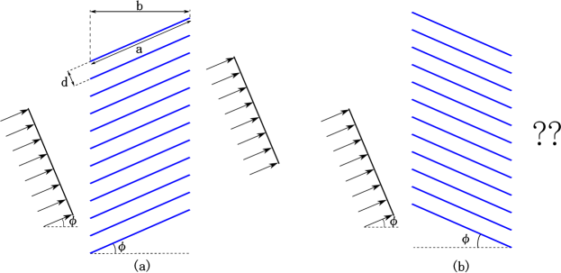
Figure 2: Figure (a) shows a grating of thin rigid strips aligned with the incident plane wave, resulting in perfect transmission. What will happen if we reverse the orientation of the slab elements as in (b)?

Extraordinary optical transmission (EOT) through metallic gratings can occur when the openings resonate in Fabry-Perot mode, which is well established although very narrow band effect. Broadband EOT, spanning from DC upwards, has been recently proposed [4] and realized [5] based on a Brewster angle effect that results from the equivalent long-wavelength properties of the grating. Aközbek et al. [6] demonstrated Brewster-like broadband extraordinary optical transmission in a thick metal plate with slits as narrow as $\lambda$/750. They showed that an order of magnitude larger transmission is obtained for very narrow slits compared to the normal-incidence Fabry-Pérot resonance transmission peaks. EOT has also been confirmed experimentally for TE and TM waves through subwavelength dielectric gratings in the microwave regime [7].

Figure 3: The single-layer grating of Fig. 1 rotated through angle $\phi$ to make a slab that is non-symmetric with respect to the incident angle.

Brewster angle total transmission is rarely observed for acoustic waves in homogeneous materials. The successful demonstration of EOT therefore raised the question of whether the same subwavelength effect can be achieved in acoustics. D’Aguanno et al. [2] answered the question in the affirmative, demonstrating theoretically and experimentally an acoustic grating that is completely transparent to sound waves. The Brewster-like effect was explained via surface impedance matching between the exterior air and the effectively rigid grating. The gaps presented by the spaces between the grating elements allows the effective impedance to be designed to produce arbitrary Brewster angle. Subsequent demonstrations of extraordinary acoustic transmission (EAT) include Qiu et al. [8] who considered a hybrid grating composed of two dissimilar grating elements different from the exterior air. Higher frequency properties of EAT gratings are discussed by Qi et al. [9], while Aközbek et al. [10] examine pass and stop-band effects for 1D phononic crystals made from repeated EAT slabs.

The mechanism behind EAT is, as noted by D’Aguanno et al. [2], impedance matching. The grating displays effective long-wavelength properties easily estimated for rigid grating elements, which allows tuning the grating porosity to achieve the desired intromission angle [2]. Maurel et al. [1] also provide a clear explanation of the phenomenon as impedance matching but in the context of acoustics of fluids with anisotropic inertia. They considered more complicated gratings comprising fluid elements and geometrical substructure, such as double layer gratings. They showed that the anisotropic effective properties of the grating can be accurately predicted using homogenization theory. This opens the door to the design of EAT gratings by varying the material properties and the geometrical details. No matter how complicated the design, homogenization theory will predict the EAT properties as long as the horizontal substructure periodicity is subwavelength. At shorter wavelength the present approach breaks down as dispersive effects come into play. Interesting nonlocal effects may be expected, as has been demonstrated for electromagnetic metamaterials comprising slanted inclusions [11]. While the geometries considered here involve waveguides of uniform width, tapered waveguides could be considered, as in [12], introducing gradients in the effective properties. However, these possibilities are beyond the scope of this paper and remain as future areas of study.

The purpose of this paper is to demonstrate EAT effects in non-symmetric gratings, of the type depicted in Fig. 3. We consider the general case in which the grating material is an acoustic fluid, the rigid SLG being a limiting case. We use homogenization theory to replace the grating by an equivalent effective medium with anisotropic density. The transmission coefficient of the equivalent uniform slab can then be obtained in closed form in terms of the original parameters, including the orientation angle of the oblique grating. Prior to this work EAT has only been considered in the context of symmetric gratings, such as in Fig. 1. While Qi et al. [13] provide experimental measurements of the effective index and effective impedance of obliquely oriented SLGs as function of wavelength, they do not report EAT effects nor do they provide analytical results for the effective properties. Based on the results of this paper it would be straightforward to estimate the effective index and effective impedance of SLGs as shown in Fig. 3.

The outline of the paper is as follows. We begin in §2 with a homogeneous model of an acoustic slab with anisotropic density, and derive explicit expressions for plane wave reflection and transmission, eqs. (5) and (6). The effective anisotropic properties are then derived in §3 using standard long-wavelength homogenization methods. Several limiting cases, including the rigid grating, are discussed in §4. Numerical examples illustrating the dependence of intromission angle and transmittivity on the slant angle $\phi$ are given in §5. Conclusions are presented in §6.

2 Acoustic transmission through a slab with anisotropic inertia

The exterior acoustic medium has density $\rho$ and sound speed $c$, with bulk modulus $K=\rho c^{2}$. The governing acoustic equations for the acoustic pressure $p$ and velocity ${\bf v}$ are

$${\bf v}=(i\omega\rho)^{-1}\nabla p,\ \ \ p=(i\omega)^{-1}K\operatorname{div}{\bf v}.$$ (1)

Time harmonic dependence $e^{-i\omega t}$ is assumed. The acoustic pressure comprises incident, reflected and transmitted plane waves as shown in Fig. 4,

$$p=p_{0}\,e^{ik\sin\theta\,x_{2}}\times\begin{cases}\big{(}e^{ik\cos\theta\,x_{1}}+Re^{-ik\cos\theta\,x_{1}}\big{)}&x_{1}\leq 0,\\ Te^{ik\cos\theta(x_{1}-b)}&x_{1}\geq b,\end{cases}$$ (2)

where $k=\frac{\omega}{c}$ and $p_{0}$ is a constant. Define for later use the acoustic impedance

$$Z_{\theta}=\frac{\rho c}{\cos\theta}.$$ (3)

We are interested in conditions for which $|T|=1$.

Figure 4: Two-dimensional configuration for the equivalent uniform slab with anisotropic density.

Consider a uniform slab of thickness $b$, bulk modulus $K_{s}$ and inertia tensor which is represented by a 2$\times$2 symmetric matrix $(\boldsymbol{\rho}=\boldsymbol{\rho}^{T})$ with elements $\rho_{ij}$, $i,j=1,2$. Specific models for anisotropic non-diagonal density tensors are discussed in §3. The equations of motion within the slab are

$${\bf v}=(i\omega\boldsymbol{\rho})^{-1}\nabla p,\ \ \ p=(i\omega)^{-1}K_{s}\operatorname{div}{\bf v}.$$ (4)

The transmission and reflection coefficients follow from Appendix A as

$$T =e^{-ikb\frac{\rho_{12}}{\rho_{22}}\sin\theta}\Big{(}\cos\frac{\omega b}{c_{\theta}}-\frac{i}{2}\Big{(}\frac{Z_{\theta}}{Z_{\theta}^{\prime}}+\frac{Z_{\theta}^{\prime}}{Z_{\theta}}\Big{)}\sin\frac{\omega b}{c_{\theta}}\Big{)}^{-1},$$ (5a)

$$R =\frac{i}{2}\Big{(}\frac{Z_{\theta}}{Z_{\theta}^{\prime}}-\frac{Z_{\theta}^{\prime}}{Z_{\theta}}\Big{)}\sin\frac{\omega b}{c_{\theta}}\Big{(}\cos\frac{\omega b}{c_{\theta}}-\frac{i}{2}\Big{(}\frac{Z_{\theta}}{Z_{\theta}^{\prime}}+\frac{Z_{\theta}^{\prime}}{Z_{\theta}}\Big{)}\sin\frac{\omega b}{c_{\theta}}\Big{)}^{-1},$$ (5b)

where

$$c_{\theta}=\Big{(}\frac{\rho_{22}}{\operatorname{det}\boldsymbol{\rho}}\Big{)}^{\frac{1}{2}}\Big{(}\frac{1}{K_{s}}-\frac{\sin^{2}\theta}{c^{2}\rho_{22}}\Big{)}^{-\frac{1}{2}},\quad Z_{\theta}^{\prime}=\Big{(}\frac{\operatorname{det}\boldsymbol{\rho}}{\rho_{22}}\Big{)}c_{\theta}.$$ (6)

The results (5)-(6) have not been previously published. Maurel et al. [1] consider the particular case of aligned inertial and slab axes $(\rho_{12}=0)$. The case of a normal acoustic fluid in the slab corresponds to $\rho_{11}=\rho_{22}$, $\rho_{12}=0$. Note that

$$R(-\theta)=R(\theta),\quad|T(-\theta)|=|T(\theta)|$$ (7)

Thus, as a function of incident angle the reflection coefficient is symmetric about $\theta=0$, but only the magnitude of the transmission coefficient is symmetric. The asymmetry as a function of $\theta$ is evident from the relation

$$\frac{T(-\theta)}{T(\theta)}=e^{i2kb\frac{\rho_{12}}{\rho_{22}}\sin\theta}.$$ (8)

A similar expression for the ratio of transmission coefficients for transmission through an anisotropic dielectric slab was derived by Castanié et al. [14, Eqs. (18) to (21)], who also considered propagation through layered anisotropic dielectric media. Note that the identity (7)₁ for the reflection coefficient is expected based on reciprocity [15].

Equation (5a) implies $|T|=1$ when the impedances match,

$$|T(\theta_{i})|=1\ \ \Leftrightarrow\ \ Z_{\theta}=Z_{\theta}^{\prime}.$$ (9)

Hence, enhanced acoustic transmittivity occurs if

$$\rho^{2}\sin^{2}\theta_{i}+(\operatorname{det}\boldsymbol{\rho})\cos^{2}\theta_{i}=\frac{K}{K_{s}}\rho\rho_{22}.$$ (10)

The value of $\theta_{i}$ satisfying this relation is the intromission angle. It is clear from $\eqref{6-56}_{2}$ that the intromission effect is symmetric in the incident angle, i.e. $|T(\pm\theta_{i})|=1$.

3 Single-layer gratings as anisotropic inertial slabs

Figure 5: A single-layer grating. The grating material is an acoustic fluid of bulk modulus $K_{0}$, density $\rho_{0}$ and volume fraction $f$. A symmetric gratings is shown on the left. On the right, the elements of the grating are rotated through angle $\phi$ to make a slab that is non-symmetric with respect to the incident angle $\theta$ of Fig. 4.

Consider first the symmetric single-layer grating (SLG) of Fig. 5 for which the grating fluid has properties $K_{0}$, $\rho_{0}$, and volume fraction $f\in[0,1]$. The effective bulk modulus $K_{s}$ and density tensor $\boldsymbol{\rho}$ of the slab follow from standard quasi-static homogenization, e.g.  [1, eq. (3)], as

$$\frac{1}{K_{s}}=\frac{f}{K_{0}}+\frac{1-f}{K},\ \ \boldsymbol{\rho}=\begin{pmatrix}\rho_{1}&0\\ 0&\rho_{2}\end{pmatrix},\ \ \frac{1}{\rho_{1}}=\frac{f}{\rho_{0}}+\frac{1-f}{\rho},\ \ \rho_{2}=f\rho_{0}+(1-f)\rho.$$ (11)

The SLG rotated through angle $\phi$ relative to the $x_{1}x_{2}$ directions as in Fig. 5 has the same effective bulk modulus $K_{s}$ while the inertia tensor becomes non-diagonal and symmetric, with

$$\boldsymbol{\rho}=\begin{pmatrix}\rho_{11}&\rho_{12}\\ \rho_{21}&\rho_{22}\end{pmatrix},\ \ \ \begin{aligned} \rho_{11}&=\rho_{1}\cos^{2}\phi+\rho_{2}\sin^{2}\phi,\\ \rho_{22}&=\rho_{1}\sin^{2}\phi+\rho_{2}\cos^{2}\phi,\\ \rho_{12}&=(\rho_{1}-\rho_{2})\sin\phi\cos\phi\ \big{(}=\rho_{21}\big{)}.\end{aligned}$$ (12)

Note that $\rho_{11},\rho_{22}>0$,

$$\rho_{12}=-\,\frac{f(1-f)(\rho-\rho_{0})^{2}}{f\rho+(1-f)\rho_{0}}\sin\phi\cos\phi\ \ \Rightarrow\ \ \begin{cases}\rho_{12}<0&\text{if}\ \phi>0,\\ \rho_{12}>0&\text{if}\ \phi<0,\\ \rho_{12}=0&\text{if}\ \phi=0,\end{cases}$$ (13)

while $\operatorname{det}\boldsymbol{\rho}=\rho_{1}\rho_{2}$ and $\operatorname{tr}\boldsymbol{\rho}=\rho_{1}+\rho_{2}$ are independent of $\phi$. The relative phase of the transmitted wave for incidence at $\pm\theta$, eq. (8), becomes, using $b=a\cos\phi$,

$$\frac{T(-\theta)}{T(\theta)}=e^{-i2ka\sin\phi\sin\theta\,\big{(}\frac{\rho_{2}-\rho_{1}}{\rho_{2}+\rho_{1}\tan^{2}\phi}\big{)}}.$$ (14)

The phase difference in (14) between $T(\theta)$ and $T(-\theta)$ can be understood as follows. First, the term $-2ka\sin\phi\sin\theta$ has clear geometrical meaning. Referring to Figure 6, note that $k\sin\theta$ is the conserved horizontal wavenumber, while $a\sin\phi$ is the horizontal path length, resulting in the phase advance/delay of $\pm ka\sin\phi\sin\theta$ for incidence at $\pm\theta$. The additional factor, $\frac{\rho_{2}-\rho_{1}}{\rho_{2}+\rho_{1}\tan^{2}\phi}$, which is positive but less than unity on account of the fact that $\rho_{2}>\rho_{1}$, arises from acoustic propagation in the grating elements. This results in a smaller phase effect than that of the rigid limit $(\rho_{2}\gg\rho_{1})$. The phase term obviously becomes zero in the symmetric limit $\phi=0$. Note, however, that for the fluid grating the phase also tends to zero as $\phi\to\frac{\pi}{2}$.

Figure 6: Relative phase of the transmission coefficients for $\pm\theta$.

Using the explicit formulae for the anisotropic density tensor, the impedance matching condition (10) becomes

$$|T(\theta_{i})|=1\ \ \Leftrightarrow\ \ \boxed{\cos^{2}\theta_{i}=\frac{\big{(}\frac{\rho_{2}-\rho_{1}}{\rho}\cos^{2}\phi+\frac{\rho_{1}}{\rho}\big{)}\frac{K}{K_{s}}-1}{\frac{\rho_{1}\rho_{2}}{\rho^{2}}-1}}$$ (15)

This shows the explicit dependence on the orientation angle $\phi$. In particular, it implies that $\partial\theta_{i}/\partial\phi>0$ since $\rho_{2}-\rho_{1}>0$ and $\rho_{1}\rho_{2}>\rho^{2}$ for $\rho_{0}\neq\rho$.

4 Limiting cases and generalizations

The intromission angle for the single-layer grating of Fig. 4 is given by eq. (15). Here we consider its behavior for some limits of the parameters, such as rigid grating elements. The limiting case of $\phi=0$ was considered by [1], although they do not provide a simple full-transmission condition analogous to (15) with $\phi=0$.

4.1 Rigid grating elements

If the grating element is much stiffer than the background fluid, then in the limit $K/K_{0}\to 0$ (15) becomes

$$|T(\theta_{i})|=1,\ \frac{K}{K_{0}}=0,\ \ \Leftrightarrow\ \ {\cos^{2}\theta_{i}=\frac{(1-f)\frac{\rho_{22}}{\rho}-1}{\frac{\rho_{1}\rho_{2}}{\rho^{2}}-1}}.$$ (16)

The case of a fixed rigid grating is obtained in the dual limit of large stiffness and density, i.e.

$$|T(\theta_{i})|=1,\ \frac{K}{K_{0}}=0,\ \frac{\rho}{\rho_{0}}=0,\ \ \Leftrightarrow\ \ \boxed{\cos\theta_{i}=(1-f)\cos\phi}$$ (17)

This case, which we call the rigid limit, is of particular interest. It is easily realized if the background acoustic medium is air.

In the rigid limit (17) we have (see eq. (6)) $c_{\theta}=c\cos\phi$, and the transmission coefficient of (5a) simplifies to

$$T(\theta)=e^{ika\sin\phi\sin\theta}/\Big{(}\cos ka-\frac{i}{2}\big{(}\frac{\cos\theta}{\cos\theta_{i}}+\frac{\cos\theta_{i}}{\cos\theta}\big{)}\sin ka\Big{)}.$$ (18)

Hence,

$$|T(\theta)|=\cos\gamma,\ \ |R(\theta)|=\sin\gamma,\ \ \gamma=\tan^{-1}\Big{(}\frac{1}{2}\big{(}\frac{\cos\theta}{\cos\theta_{i}}-\frac{\cos\theta_{i}}{\cos\theta}\big{)}\sin ka\Big{)}$$ (19)

and the relative phase of the transmission coefficients for $\pm\theta$ is

$$\frac{T(-\theta)}{T(\theta)}=e^{-i2ka\sin\phi\sin\theta}.$$ (20)

The reason for the phase difference $-2ka\sin\phi\sin\theta$ is evident from Fig. 6.

4.2 Transmission at normal incidence: $\theta_{i}=0$

The intromission angle is identically zero if

$$|T(0)|=1\ \ \Leftrightarrow\ \ \boxed{\frac{K}{K_{0}}=\frac{\rho_{0}^{2}-(1-f)^{2}(\rho_{0}-\rho)^{2}\cos^{2}\phi}{\rho\rho_{0}+f(1-f)(\rho_{0}-\rho)^{2}\cos^{2}\phi}\leq\frac{\rho_{0}}{\rho}}$$ (21)

This is a rather interesting identity: it indicates that the required impedance ratio $\sqrt{K\rho/K_{0}\rho_{0}}$ depends on the density ratio and the ”‘environmental” parameters $f$ and $\phi$ but not on the relative bulk moduli. If any one of the three conditions $f=1$, $\phi=\frac{\pi}{2}$ or $\rho_{0}=\rho$ holds then (21) reduces to the expected one-dimensional impedance matching condition $K_{0}\rho_{0}=K\rho$. However, when $f\neq 1$ and $\rho_{0}\neq\rho$ eq. (21) implies that the grating material must have higher impedance than the background fluid.

Assume further that full transmission at $\theta_{i}=0$ corresponds to $\phi=0$, then (15) (or (21)) requires

$$\left.\begin{aligned} |T(0)|&=1,\\ \phi&=0,\end{aligned}\right\}\ \ \Leftrightarrow\ \ \frac{K}{K_{0}}=\frac{\rho_{0}^{2}-(1-f)^{2}(\rho_{0}-\rho)^{2}}{\rho\rho_{0}+f(1-f)(\rho_{0}-\rho)^{2}}.$$ (22)

Now vary $\phi$, with (22) satisfied, then eq. (15) becomes

$$|T(\theta_{i})|=1\ \ \Leftrightarrow\ \ \sin\theta_{i}=\sqrt{\frac{(1-f)\rho_{0}}{f\rho+(1-f)\rho_{0}}\Big{(}\frac{\rho_{0}-\rho}{\rho_{0}+\rho}\Big{)}}\,\sin\phi.$$ (23)

This provides a possible active model for changing the angular receptivity of the slab by rotating the elements of the single-layer grating.

4.3 Zigzag structures

A zigzag structure, as shown in Fig. 7, here means one that is made from layers in series, each layer being a SLG with grating elements oriented at $\phi$ or $-\phi$. The only difference between adjacent layers is that the effective density $\rho_{12}$ changes sign. Let $b_{+}$ $(b_{-})$ be the combined thickness of the layers with orientation $+\phi$ $(-\phi)$, so that the total thickness is $b=b_{+}+b_{-}$.

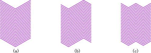
Figure 7: Zigzag structures are SLGs in series with alternating orientations $\pm\phi$.

The transmission coefficient is

$$T(\theta)=e^{-ik(b_{+}-b_{-})\frac{\rho_{12}}{\rho_{22}}\sin\theta}\Big{(}\cos\frac{\omega b}{c_{\theta}}-\frac{i}{2}\Big{(}\frac{Z_{\theta}}{Z_{\theta}^{\prime}}+\frac{Z_{\theta}^{\prime}}{Z_{\theta}}\Big{)}\sin\frac{\omega b}{c_{\theta}}\Big{)}^{-1},$$ (24)

the reflection coefficient is given by eq. (5b), and the other parameters in (24) are as before. The three examples of zigzag structures in Fig. 7 all have $b_{+}=b_{-}$ and therefore $T(-\theta)=T(\theta)$ in each case.

5 Numerical examples

The examples presented use non-dimensional parameters as far as possible; in particular the frequency is defined by $kd$. The length of the grating elements is $a=20d$, see Fig. 5, and the total slab thickness $b$ depends on the orientation angle through $b=a\cos\phi$. All results shown were generated with COMSOL using periodic boundary conditions to simulate wave transmission through an infinitely periodic structure.

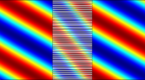
(a) $f=0.5$, $kd=0.25$

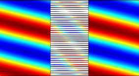
(e) $f=0.75$, $kd=0.25$

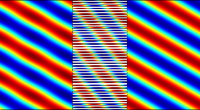
(b) $f=0.5$, $kd=0.5$

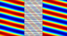
(f) $f=0.75$, $kd=0.5$

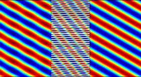
(c) $f=0.5$, $kd=0.75$

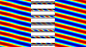
(g) $f=0.75$, $kd=0.75$

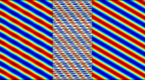
(d) $f=0.5$, $kd=1$

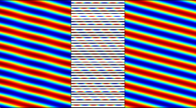
(h) $f=0.75$, $kd=1$

Figure 8: Total pressure plots at different frequencies for a symmetric $(\phi=0)$ slab of rigid elements. The incident angle is taken to be the intromission angle $\theta_{i}=\cos^{-1}(1-f)$, where $f=0.5$ $\Rightarrow\theta_{i}=60^{\circ}$ in (a) through (d) while $f=0.75$ $\Rightarrow\theta_{i}=41.4^{\circ}$ in (e) through (h). The values of $kd$ range from $0.25$ to $1.0$, as indicated.

5.0.1 Rigid grating elements

We begin with a symmetric slab of rigid elements, $\phi=0$, in Figure 8. The plots show total pressure for waves incident at the intromission angle for two different values of the filling fraction, $f=0.5$ and $f=0.75$, at four frequencies at or below $kd=1$. The plots clearly show total transmission for frequencies $kd\ll 1$.

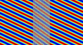
(a) $\phi=30^{\circ}$, $f=0.5$

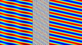
(c) $\phi=30^{\circ}$, $f=0.75$

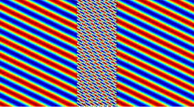
(b) $\phi=-30^{\circ}$, $f=0.5$

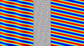
(d) $\phi=-30^{\circ}$, $f=0.75$

Figure 9: Total pressure plots for incidence at the intromission angle of a slanted grating of rigid elements, $\theta_{i}=\cos^{-1}\big{(}(1-f)\cos\phi\big{)}$, $\phi=\pm 30^{\circ}$, at frequency $kd=1$. Plots (a) and (b) show the full pressure field for filling fraction $f=0.5$, while (c) and (d) are for higher filling fraction $f=0.75$.

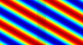
(a) $\phi=60^{\circ}$, $kd=0.25$

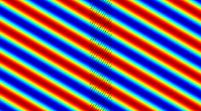
(c) $\phi=60^{\circ}$, $kd=0.5$

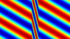
(b) $\phi=-60^{\circ}$, $kd=0.25$

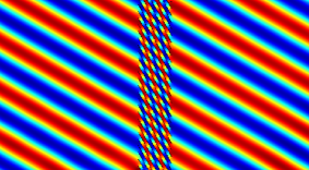
(d) $\phi=-60^{\circ}$, $kd=0.5$

Figure 10: Wave transmission through a SLG of thin rigid elements (volume fraction $f=0+$) oriented at $\phi=\pm 60^{\circ}$ for incidence at the intromission angle $\theta_{i}=60^{\circ}$.

As noted above, full transmission through an asymmetric grating of elements oriented at angle $\phi$ can be obtained at both $\theta_{i}$ and $-\theta_{i}$. In the numerical experiments shown in Fig.  9 we change the direction of rotation of slab elements instead of changing the incident direction, i.e., using $\pm\phi$ instead of $\pm\theta$. Figure 9 shows that the pressure amplitude transmitted through the slab for $\phi$ is the same as for $-\phi$. The transmitted phases are clearly different; the phase effect is easier to see in Fig.  9 for the example with lower filling fraction. In the limit of zero but still finite filling fraction, $f=0+$, the rigid element SLG acts like a comb, totally transparent for incidence at $\theta_{i}=\pm\phi$, as illustrated in Figure 10 with a zoom-in shown in Fig.  11. The phase difference between incidence at $\theta_{i}=+\phi$ and $\-\phi$ is most dramatic in this limit of thin rigid grating elements. This proves the original assertion about what happens in Fig.  2(b).

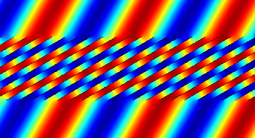
Figure 11: Zoomed-in view of the phase difference in plot (b) of Figure 10.

As a final example of a grating with rigid elements, Fig. 12 shows the computed reflection and transmission coefficients for three different slanted gratings. The intromission angle in each case was chosen to be $\theta_{i}=60^{\circ}$ which constrains the orientation angle $\phi$ and the volume fraction $f$ to satisfy $(1-f)\cos\phi=\frac{1}{2}$, see eq.  (17). Figure 12 indicates that the transmission spectrum does not change significantly as long as the relation between $\theta_{i}$, $\phi$ and $f$ is obeyed.

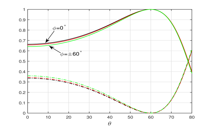
Figure 12: Full transmission at $\theta_{i}=60^{\circ}$ for three different rigid SLGs with elements oriented at $\phi=0^{\circ}$, $30^{\circ}$ and $60^{\circ}$. The solid and dashed curves show $|T|^{2}$ and $|R|^{2}$, respectively. The black, red, and green curves are for the cases $\phi=0^{\circ}$, $\pm 30^{\circ}$ and $\pm 60^{\circ}$, respectively. The frequency is $kd=0.25$.

5.0.2 Acoustic grating elements

The material properties of the gratings are selected so that the intromission angle is zero when the grating elements are symmetric, i.e. $\theta_{0}=0$ for $\phi=0$, and we consider the change in properties as the elements are subsequently rotated to $\phi>0$. The background acoustic medium is assumed to be water, $\rho=1000$ kg/m³, $c=1500$ m/s, and $K=2.25$ GPa. We first consider a denser fluid, $\rho_{0}=10\rho$, at volume fraction $f=0.3$, then equation (22) yields $K_{0}=1.008$ GPa, guaranteeing that a wave of normal incidence has full transmission for $\phi=0^{\circ}$. We then vary $\phi$, with all other material parameters fixed, to calculate the intromission angle for each $\phi$ according to eq. (23). Figure 13 shows how the intromission angle changes with $\phi$. Notice that $\phi$ can be positive or negative so that the gratings can rotate in two directions. The full field shown in Fig.  14 illustrates the phase transfer across the SLG. This is clearly more complicated than in the rigid case, where the acoustic propagation is along parallel waveguides. The interaction of the two fluids in the SLG is particularly evident in Fig. 14(c).

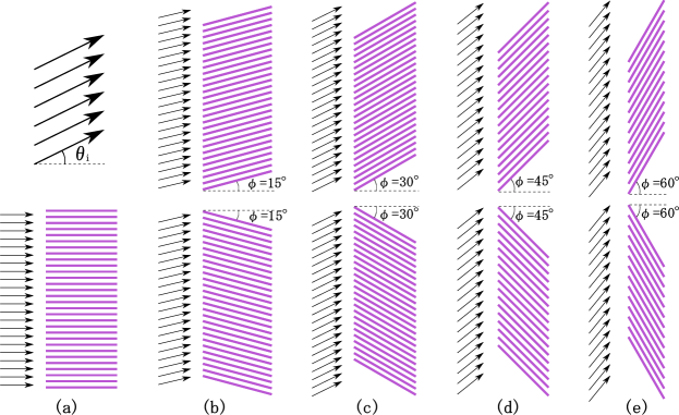
Figure 13: The intromission angle changes with $\pm\phi$ for an acoustic grating with filling fraction $f=0.3$ subject to the constraint that (a) $\theta_{i}=0^{\circ}$ for $\phi=0$. The intromission angle $\theta_{i}$ in the other cases is: (b) $13.3^{\circ}$, (c) $26.3^{\circ}$, (d) $38.8^{\circ}$, (e) $50.1^{\circ}$.

In the previous example the grating elements were chosen as denser than the background (water) and it was found that the grating had to be less stiff (lower bulk modulus) than water. Conversely, if we consider a SLG using a fluid that is lighter than the background, the same constraint that the intromission angle is zero for symmetric alignment, $\theta_{i}=0$ at $\phi=0$, requires that the fluid is stiffer than water. For instance, eq.  (22) is satisfied with $f=0.3$, $\rho_{0}=0.45\rho$ and $K_{0}=21.29$ GPa, so that the intromission angle is zero for the symmetric configuration $\phi=0$. Figure 15 shows how the intromission angle changes with $\phi$ for this grating. Figure 16 show the full field for $\phi=\pm 30^{\circ}$ and $\phi=\pm 60^{\circ}$. It is instructive to compare these results with those for the other fluid in Fig. 14.

It is possible, in principle, to design materials with low density $\rho_{0}<\rho$ and high stiffness $K_{0}>K$. Metal foams, e.g. Duocel®aluminum foam, can have very low density $\rho_{0}\ll\rho$ and relatively high stiffness, however, the random structure usually limits the effective bulk modulus to be less than that of water. Simultaneously ultra-light and ultra-stiff materials are obtained using thin lattice structures with ordered periodicity [16]. These materials possess significant shear modulus, i.e. the Poisson’s ratio is not close to $\frac{1}{2}$, which implies they support both shear and longitudinal waves. By carefully selecting the unit cell one can achieve a one-wave fluid like material with properties $\rho_{0}=\rho$ and $K_{0}=K$ of water, specifically known as Metal Water [17]. The low shear rigidity is ensured by using very thin members with large flexural compliance. The metal water structure, designed to have quasistatic properties of water, also exhibits interesting band structure which makes it a narrow-band negative index material [18]. The generalization of the metal water structure is a class of metallic pentamode materials with low-shear and design specific density and stiffness, which could in principle achieve desired values of $\rho_{0}$, $K_{0}$.

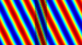
(a) $\phi=30^{\circ}$

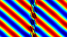
(c) $\phi=60^{\circ}$

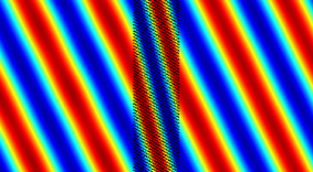
(b) $\phi=-30^{\circ}$

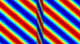
(d) $\phi=-60^{\circ}$

Figure 14: Total pressure plots for some configurations from Fig.  13 at frequency $kd=0.25$.

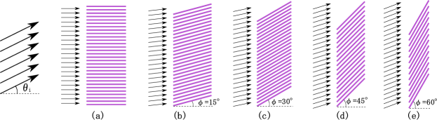
Figure 15: The intromission angle is constrained to be zero for symmetric alignment $(\phi=0)$ for a grating with fluid less dense and stiffer than the background, (a). For filling fraction $f=0.3$, the grating elements are rotated by angle $\phi$ and the intromission angle $\theta_{i}$ becomes (b) $6.5^{\circ}$, (c) $12.5^{\circ}$, (d) $17.6^{\circ}$, (e) $21.4^{\circ}$.

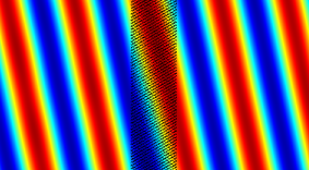
(a) $\phi=30^{\circ}$

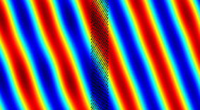
(c) $\phi=60^{\circ}$

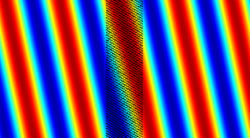
(b) $\phi=-30^{\circ}$

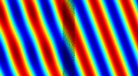
(d) $\phi=-60^{\circ}$

Figure 16: Total pressure plots for some configurations from Fig.  15 at frequency $kd=0.25$.

6 Conclusions

Our main result is eq. (15) which gives the intromission angle for the single-layer grating of Fig. 3. While it is known that EAT can be understood as impedance matching in the context of acoustics of fluids with anisotropic inertia [1] the present results show that this analogy extends further to include asymmetric gratings. The principal axes of the anisotropic inertia are not necessarily aligned with the slab axes (Fig. 5) which introduces asymmetry in the phase of the transmitted wave as a function of incidence angle $\pm\theta$. These seemingly unusual results for total transmission can be easily understood when the grating elements are rigid. Thus, any angle of intromission can be obtained with thin rigid elements by orienting them to the desired value of $\theta_{i}$, a simple comb-like effect. Surprisingly, full transmission is also achieved at incident angle $-\theta_{i}$, see Fig. 10.

The rigid grating with thin slanted elements illustrates the geometrical acoustics nature of the EAT phenomenon. However, the simultaneous EAT effect at orientations $\pm\phi$ emphasizes that the underlying phenomenon is “geometrical impedance matching”. The term geometrical impedance matching is introduced to signify the flux condition across the interface, as compared with the phase matching (Snell’s or Descartes’ law) in the transverse direction. Thus, geometrical impedance matching leads directly to the identity (17) for the rigid grating. However, one needs a full wave approach in order to arrive at the more general result of eq. (15) for the intromission angle in the presence of an acoustic fluid grating. Despite this, the simplicity of the identity eq. (15) for the intromission angle is remarkable.

Appendix

A Solution for an anisotropic inertial slab

The slab properties are bulk modulus $K_{s}$ and 2$\times$2 inertia matrix $\boldsymbol{\rho}=\boldsymbol{\rho}^{T}$. Define the state vector

$${\bf u}=\begin{pmatrix}v_{1}\\ -p\end{pmatrix},$$ (A.1)

and consider solutions with constant horizontal phase such that ${\bf u}$ has the form

$${\bf u}(x_{1},x_{2})={\bf U}(x_{1})e^{ik\sin\theta\,x_{2}}.$$ (A.2)

Then ${\bf U}(x_{1})$ satisfies

$$\frac{\operatorname{d}{\bf U}}{\operatorname{d}x_{1}} =i\omega{\bf A}{\bf U}\ \ \text{where}$$ (A.3)

$${\bf A} =\frac{\sin\theta}{c}\frac{\rho_{12}}{\rho_{22}}{\bf I}-{\bf B},\quad{\bf B}=\begin{pmatrix}0&\frac{1}{K_{s}}-\frac{\sin^{2}\theta}{c^{2}\rho_{22}}\\ \frac{\operatorname{det}\boldsymbol{\rho}}{\rho_{22}}&0\end{pmatrix}$$ (A.4)

and ${\bf I}$ is the identity matrix. Note that the matrix ${\bf A}$ is independent of the frequency $\omega$.

Define the propagator matrix, ${\bf M}(x)$, as the solution of

$$\frac{\operatorname{d}{\bf M}(x)}{\operatorname{d}x}={i\omega}{\bf A}{\bf M}\ \ \text{with}\ {\bf M}(0)={\bf I}.$$ (A.5)

Note that $\operatorname{det}{\bf M}=1$ [19]. The property ${\bf A}^{T}={\bf J}{\bf A}{\bf J}$ where the 2$\times$2 matrix ${\bf J}$ has zeroes on the diagonal and unity off diagonal, implies that the Hermitian conjugate satisfies ${\bf M}^{\dagger}={\bf J}{\bf M}^{-1}{\bf J}$ and hence ${\bf M}^{-1}(x)={\bf J}{\bf M}^{\dagger}(x){\bf J}={\bf M}(-x)$.

We consider slabs with uniform properties in $x\in[0,b]$, so that

$${\bf M}(b)=e^{{i\omega}b{\bf A}}.$$ (A.6)

This explicit form of the propagator matrix simplifies, using eqs. (A.4) and (A.6) and the property that $c_{\theta}^{-1}{\bf B}$ is a square root of the identity, to give

$${\bf M}(b)=\Big{(}\cos\frac{\omega b}{c_{\theta}}\,{\bf I}-\frac{i}{c_{\theta}}\sin\frac{\omega b}{c_{\theta}}\,{\bf B}\Big{)}\,e^{ikb\frac{\rho_{12}}{\rho_{22}}\sin\theta},$$ (A.7)

where

$$c_{\theta}=\big{(}-\operatorname{det}{\bf B}\big{)}^{-1/2}.$$ (A.8)

Based on eqs. (2) and (A.2),

$${\bf U}(0-)=p_{0}\begin{pmatrix}Z_{\theta}^{-1}(1-R)\\ -1-R\end{pmatrix},\quad{\bf U}(b+0)=p_{0}T\begin{pmatrix}Z_{\theta}^{-1}\\ -1\end{pmatrix},$$ (A.9)

The continuity conditions at $x_{1}=0$ and $x_{1}=b$ require the normal velocity $v_{1}$ and the pressure $p$ to be continuous, that is ${\bf U}(0+)={\bf U}(0-)$ and ${\bf U}(b-0)={\bf U}(b+0)$. Hence, with $M_{ij}=M_{ij}(b)$,

$$T\begin{pmatrix}Z_{\theta}^{-1}\\ -1\end{pmatrix}=\begin{pmatrix}M_{11}&M_{12}\\ M_{21}&M_{22}\end{pmatrix}\begin{pmatrix}Z_{\theta}^{-1}(1-R)\\ -1-R\end{pmatrix}$$ (A.10)

The transmission and reflection coefficients follow from (A.10) as

$$T =2\big{(}M_{11}+M_{22}+Z_{\theta}M_{12}+Z_{\theta}^{-1}M_{21}\big{)}^{-1},$$ (A.11a)

$$R =1-\big{(}M_{22}+Z_{\theta}M_{12}\big{)}\ T.$$ (A.11b)

Using the explicit solution for ${\bf M}(b)$ from (A.7) and (A.8) yields (5).

—————————————–