Measurement of the cosmic-ray energy spectrum above $10^{16}$ eV with the LOFAR Radboud Air Shower Array

Abstract

The energy reconstruction of extensive air showers measured with the LOFAR Radboud Air Shower Array (LORA) is presented in detail. LORA is a particle detector array located in the center of the LOFAR radio telescope in the Netherlands. The aim of this work is to provide an accurate and independent energy measurement for the air showers measured through their radio signal with the LOFAR antennas. The energy reconstruction is performed using a parameterized relation between the measured shower size and the cosmic-ray energy obtained from air shower simulations. In order to illustrate the capabilities of LORA, the all-particle cosmic-ray energy spectrum has been reconstructed, assuming that cosmic rays are composed only of protons or iron nuclei in the energy range between $\sim 2\times 10^{16}$ and $2\times 10^{18}$ eV. The results are compatible with literature values and a changing mass composition in the transition region from a galactic to an extragalactic origin of cosmic rays.

1 Introduction

The quest for the origin of cosmic rays is one of the most fundamental problems in Astroparticle Physics [1, 2, 3]. Since the discovery of these highly energetic particles more than a century ago, numerous measurements of several of their properties have been made, using sophisticated instruments (see e.g. Ref. [4] for a review). However, the exact nature of their sources still remains an open question. The search is mainly hindered due to the fact that cosmic rays, being charged particles, are scattered or deflected by the Galactic and inter-galactic magnetic fields during their propagation to the Earth, making it extremely difficult to reconstruct the direction of their sources. Nevertheless, observed cosmic-ray properties like the energy spectrum and composition have been used to understand and characterize the properties of the sources such as their Galactic or extragalactic nature, the cosmic-ray production spectrum and the power injected into cosmic rays (see e.g. Refs. [5, 6, 7, 8, 9, 10, 11] for recent reviews).

LOFAR, the LOw Frequency ARray, is an astronomical radio telescope [12]. It has been designed to measure the properties of cosmic rays above $\sim 10^{16}$ eV by detecting radio emission from extensive air showers in the frequency range of $10-240$ MHz [13]. One of the main goals of the LOFAR key science project Cosmic Rays is to provide an accurate measurement of the mass composition of cosmic rays in the energy range between $\sim 10^{16}$ and $\sim 10^{18}$ eV, a region where the transition from Galactic to extragalactic cosmic rays is expected. This is being carried out by measuring the depth of the shower maximum ($X_{\mathrm{max}}$), using a technique based on the reconstruction of the two-dimensional radio intensity profile on the ground [14, 15]. Another focus of the LOFAR cosmic-ray measurements is to understand the nature and production mechanisms of the radio emission from air showers. This is done by measuring various properties of the radio signals in great detail such as their polarization properties, the radio wave front and relativistic time compression effects on the emission profile [16, 17, 18].

In order to assist the radio measurement of air showers with LOFAR, we have built a particle detector array LORA (LOFAR Radboud Air Shower Array) in the center of LOFAR [19]. Its main objectives are to trigger the read-out of the LOFAR radio antennas to register radio signals from air showers, and to provide basic air shower parameters such as the position of the shower axis as well as the energy and the arrival direction of the incoming cosmic-ray. These parameters are used to cross-check the reconstruction of air shower properties, based on the measured radio signals. Currently, given the lack of an absolute calibration of the radio signals, the cosmic-ray energy is estimated through the reconstruction of the particle data. Therefore, an accurate energy reconstruction with LORA is essential for a proper understanding of the air showers measured with LOFAR.

In this article, we describe in detail the various steps of the energy reconstruction and present the cosmic-ray energy spectrum above $\sim 10^{16}$ eV as measured with LORA. The article is organized as follows. A short description of the set-up will be given in Section 2 followed by a description of the data analysis technique in Section 2. The various steps involved in the Monte-Carlo simulation studies of the array will be described in Section 4, and a comparison between measurements and simulations for some of the air shower properties will be given in Section 5. In Sections 6 and 7, the energy calibration, the uncertainties in the reconstructed energies, and reconstructed cosmic-ray intensity will be described. The measured cosmic-ray spectrum and a comparison with the measurements of other experiments will be presented in Section 8, followed by a short conclusion and a future outlook.

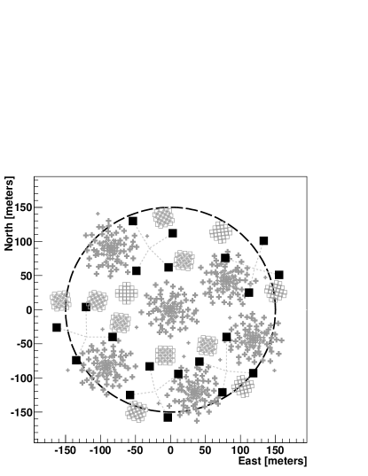
Figure 1: Layout of the LORA array in the LOFAR core. The filled black squares represent the LORA detectors, the crosses the LOFAR low-band antennas and the empty squares the high-band antennas. The dashed circle in the figure illustrates the fiducial area of a radius of $150$ m, which is used in the analysis.

2 LORA experimental set-up and operation

LORA (the LOFAR Radboud Air Shower Array) consists of an array of 20 plastic scintillation detectors of size $\sim 0.95~{}\mathrm{m}\times~{}0.95$ m each, distributed over a circular area with a diameter of $\sim 320$ m in the center of LOFAR [19]. The array is subdivided into $5$ units, each comprising of 4 detectors. The detectors have a spacing between $50-100$ m, and have been designed to measure cosmic rays with energies above $\sim 10^{16}$ eV. The array is co-located with six LOFAR stations. The layout of the array is shown in Figure 1. The data acquisition in each unit is controlled locally. A local trigger condition of 3 out of 4 detectors is set for each unit, and an event is accepted for a read-out of the full array when at least one unit has been triggered. A high-level trigger for the LOFAR radio antennas is formed when at least 13 out of the 20 detectors have measured a signal above threshold. More technical details can be found in Ref. [19].

3 Data selection and analysis

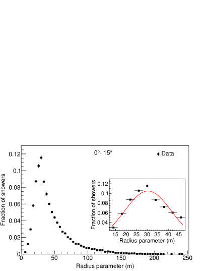
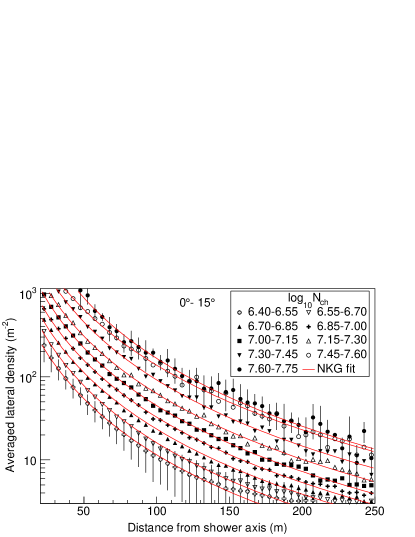
Figure 2: Left: Normalized distribution of radius parameter, $r_{\mathrm{M}}$, for the measured showers with reconstructed size $\log_{10}N_{\mathrm{ch}}>6.40$ and zenith angles in the range $0^{\circ}-15^{\circ}$. The inset shows a Gaussian fit (represented by the line) to the distribution around the maximum. Right: Averaged lateral distribution of measured showers with a reconstructed size in the range of $6.40<\log_{10}N_{\mathrm{ch}}<7.75$. Only uncertainties for the uppermost and the lower-most distribution are shown. The lines represent fits of an NKG function, keeping the shower age parameter fixed at $s=1.7$.

Data collected with the LORA array since its first science operation in June 2011 until October 2014 are used. Only data collected in periods with all 20 detectors in operation will be considered. This amounts to a total of $706.9$ days of data. For the analysis, only showers that trigger a minimum of $5$ detectors will be considered, which corresponds to a total of $1,861,045$ air showers.

For every measured shower, the signal arrival time and the energy deposit in each detector are recorded. The relative signal arrival times between the detectors are used to reconstruct the arrival direction of the primary cosmic ray. The energy deposits are used to reconstruct the position of the shower axis and the shower size (the effective number of charged particles at the ground). The latter is determined in terms of the number of vertical equivalent charged particles, which may also include converted photons in addition to the dominant charged particles - electrons and muons. The shower axis position and the shower size are determined simultaneously by fitting a lateral density distribution function to the measured two-dimensional distribution of particle densities, projected into the shower plane. The particle density in each detector is obtained by first dividing the track-length-corrected energy deposition by the energy deposition of a single particle obtained from calibration, and then by further dividing by the projected area of the detector in the shower plane. The lateral density distribution of an air shower is generally described by the Nishimura-Kamata-Greisen (NKG) function which is given by [20, 21]

$$\centering\rho(r)=N_{\mathrm{ch}}C(s)\left(\frac{r}{r_{\mathrm{M}}}\right)^{s-2}\left(1+\frac{r}{r_{\mathrm{M}}}\right)^{s-4.5},\@add@centering$$ (1)

where $\rho(r)$ represents the particle density in the shower plane at a radial distance $r$ from the shower axis, $N_{\mathrm{ch}}$ is the shower size, $s$ is shower age or lateral shape parameter and $r_{\mathrm{M}}$ is the radius parameter which is basically a measure of the lateral spread of the shower. The function $C(s)$ is given by

$$\centering C(s)=\frac{\Gamma(4.5-s)}{2\pi r_{\mathrm{M}}^{2}\Gamma(s)\Gamma(4.5-2s)}.\@add@centering$$ (2)

In the case of LORA, the value of $r_{\mathrm{M}}$ is determined from the fit along with $N_{\mathrm{ch}}$ and the position of the shower axis. The parameter $s$ is kept constant at a value of $1.7$ throughout the fitting process. Simultaneous fitting of both $r_{\mathrm{M}}$ and $s$ results in fits of poorer quality. Simulation studies have shown that keeping $s$ constant gives better results than keeping $r_{\mathrm{M}}$ constant [22]. The fitting procedure is repeated three times with the output of each fit taken as starting values for the next iteration. Details about the minimization procedure and the choice of starting values, as well as the reconstruction of the arrival direction of the primary particle are described in Ref. [19].

All showers that trigger at least $5$ detectors with a minimum of $1$ particle m^-2 are allowed to pass through the reconstruction algorithm, and their shower parameters are calculated. Furthermore, only showers whose reconstructed position of the shower axis falls within $150$ m from the center of the array are selected. The normalized distribution of $r_{\mathrm{M}}$ values for the selected showers with reconstructed sizes $\log_{10}N_{\mathrm{ch}}>6.40$ and reconstructed zenith angles in the range of $0^{\circ}-15^{\circ}$ are shown in Figure 2 (left panel). The inset shows a closer view of the distribution around the maximum value between $12$ and $48$ m, and a Gaussian fit to the distribution. The fit gives a peak value of $r_{\mathrm{M}}=30.33\pm 0.13$ m. Figure 2 (right panel) shows the averaged lateral distributions of the measured showers for different reconstructed size bins in the range of $6.40<\log_{10}N_{\mathrm{ch}}<7.75$ for zenith angle between $0^{\circ}$ and $15^{\circ}$. The distributions include events that passed through the same selection cuts applied in the left panel of Figure 2 and have $r_{\mathrm{M}}$ values in the range of $10-200$ m. The averaged distributions are obtained by stacking together the lateral distributions of all individual showers contained in each size bin. The lines in the plot represent the fits to the data using (1). To avoid clumsiness of the plots, uncertainties are shown only for the size bins of $\log_{10}N_{\mathrm{ch}}=6.40-6.55$ and $\log_{10}N_{\mathrm{ch}}=7.60-7.75$. However, all the respective uncertainties are taken into account in the fitting procedure. The values of $r_{\mathrm{M}}$ obtained from the fits are in the range of $23-31$ m.

The shower size gives a good measure of the energy of the primary cosmic-ray particle, initiating the air shower. Therefore, the shower size distribution should reflect the energy distribution of the cosmic rays at size values where the primary energy is above the detector threshold. Figure 3 shows the distribution of reconstructed shower sizes for all the measured showers that passed through the various trigger and quality cuts applied in the analysis. This corresponds to a total of $322,664$ air showers. The distribution shows a steep rise as $N_{\mathrm{ch}}$ increases which is due to the sharp increase in the detector acceptance (see section 4) as function of the primary energy. After reaching a maximum, the distribution falls off steeply which is due to the power-law behavior of the cosmic-ray spectrum. The peak of the total distribution gives the shower size threshold of the detector array. Fitting a Gaussian function around the peak gives a value of $\log_{10}N_{\mathrm{ch}}=5.92$. Also shown in Figure 3 are the reconstructed size distributions for four zenith angle bins: $0^{\circ}-15^{\circ}$, $15^{\circ}-24^{\circ}$, $24^{\circ}-30^{\circ}$, and $30^{\circ}-35^{\circ}$. The parameterization of the cosmic-ray energy will be determined separately for each zenith angle bin (see Section 6). All cuts applied in this analysis are summarized in Table 1.

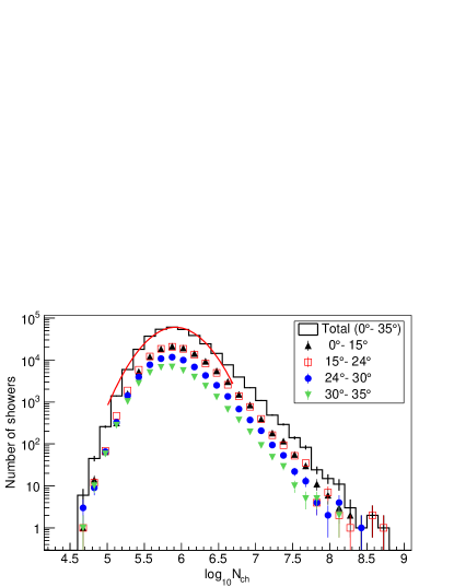
Figure 3: Measured size distribution of the air showers that have passed the quality cuts given in Table 1. The line represents a Gaussian fit to the total distribution around the peak, giving a shower size threshold of $\log_{10}N_{\mathrm{ch}}=5.92$ for the array.

Table 1: Selection cuts applied in the analysis of both the measurements and the air shower simulations.

Trigger condition:
Single unit trigger:	3/4 detectors
Analysis:	5 detectors with $\geq 1$ particle m-2
Number of leftover showers:	$1,861,045$
Quality cuts:
Zenith angle:	$\theta<35^{\circ}$
Position of the shower axis:	$<150$ m from array center
Radius parameter:	$10~{}\mbox{m}<r_{\mathrm{M}}<200~{}\mbox{m}$
Number of leftover showers:	$322,664$

4 Simulations

Detailed simulation studies have been carried out in order to understand the performance of the array and to determine various characteristics of the array, such as the trigger and reconstruction efficiencies, the reconstruction accuracies of shower parameters, the relation between reconstructed size and primary energy, and the accuracy in the energy reconstruction. In this section, the various steps involved in the simulations will be described.

4.1 Air shower simulations

Air showers are simulated using the CORSIKA simulation package (version $7.4387$) [23]. The interactions of hadronic particles in the Earth’s atmosphere are treated using QGSJET-II-04 [24] at high energies and FLUKA [25] for energies below $200$ GeV. The electromagnetic interactions are treated with EGS4 [26]. The observation level of the LORA array is set to $7.6$ m above sea level. Air showers are simulated for protons and iron nuclei in the energy range of $10^{15}-10^{19}$ eV, assuming a differential energy spectrum with an index $-2$. The showers are weighted to generate a distribution with a spectral index $-3$. Zenith angles are considered in the range $0^{\circ}-45^{\circ}$. In order to reduce the excessive computing times involved in generating the showers, ‘thinning’ is applied at a level of $10^{-6}$ with optimized weight limitation [27].

4.2 Detector simulation

The generated air shower particles are fed into a detector simulation code, based on the GEANT4 package [28], which allows to calculate the total energy deposition in each detector. All properties of the detector, such as the type and the density of the scintillator material, the detector geometry as well as the effect of the aluminum plates covering the scintillator plates are included in the simulation. In order to avoid air showers not creating a trigger in the detectors due to the large detector spacing of the LORA array, an additional step is applied to each simulated shower before feeding the particles into GEANT4. Concentric rings with a radial bin size of 2 m centered around the shower axis are constructed, and the total number of particles contained in each projected ring on the ground is calculated. All particles in a ring are then distributed uniformly in a small square region of area $A_{\mathrm{s}}=(1.5\times 1.5)$ m² with a LORA detector in its center. Depending on the arrival direction of the particles, those that hit the detector are allowed to pass through GEANT4 and the total energy deposition $E_{\mathrm{dep}}$ in the detector is obtained. In the final step, the actual amount of energy that would have been deposited in the detector is obtained by applying a correction $E^{\prime}_{\mathrm{dep}}=E_{\mathrm{dep}}A_{\mathrm{s}}\cos\theta/A_{\mathrm{R}}$, where $\theta$ is the zenith angle of the shower and $A_{\mathrm{R}}/\cos\theta$ is the projected area of the ring on the ground. The somewhat larger area of $A_{\mathrm{s}}$ than the actual detector area is used to accommodate particles hitting the detector at larger zenith angles. For each simulated shower, the radial distribution of the energy deposition in the detector, averaged over the azimuthal direction in the shower plane, is constructed as a function of the distance to the shower axis. This method also automatically allows to correct for the effect of the shower thinning applied in CORSIKA as the calculation takes into account all the particles arriving at the ground.

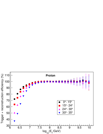
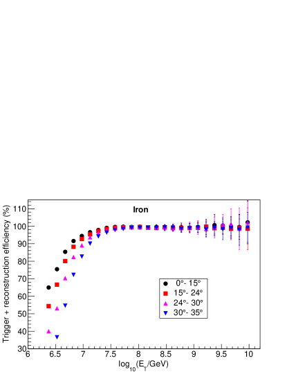
Figure 4: Combined trigger and reconstruction efficiencies obtained from the simulation of showers induced by protons (left) and iron nuclei (right) as a function of the true energy. Different symbols represent different zenith angle bins. See Section 4.4 for details.

Simulations have also been performed to calculate the energy deposition of singly charged particles in the detector. For that, muons of an energy of 4 GeV are considered. Energy depositions for vertical incident muons and for muons following a realistic (observed) arrival direction distribution are obtained. The energy deposition distribution for vertical muons gives a most probable value of $E_{\mathrm{VEM}}=5.3$ MeV, while the all-sky distribution gives $6.67$ MeV. The latter is obtained by also taking into account a noise level of $\sigma=1$ MeV, which includes a contribution from statistical noise, generated by the low number of scintillation photons producing a signal and the electronic noise. The energy deposition for the all-sky distribution is used to calibrate the distribution of the total energy deposition by single particles measured with the experiment. Details about the calibration are described in Ref. [19].

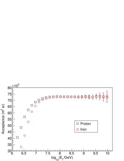
Figure 5: Total acceptance for showers induced by protons (squares) and iron nuclei (circles) obtained from simulations as function of the true energy. The acceptance is calculated for solid angles subtended within $0^{\circ}-35^{\circ}$. See Section 4.4 for details.

4.3 Reconstruction of shower parameters

Every simulated shower is assigned a random position on the ground. The position of the shower axis, and also the detector coordinates, are then projected in the shower plane. Based on the distance of the detector from the position of the shower axis in the shower plane, the amount of energy deposited in the detector is calculated from the radial distribution of energy deposition given by the simulation. To make the simulation study consistent with the analysis of the measured data, the number of particles hitting the detectors is obtained in units of VEM (vertical equivalent muons). This is done by first dividing the track-length-corrected energy deposition $E^{\prime}_{\mathrm{dep}}\cos\theta$ by $E_{\mathrm{VEM}}$ to obtain the mean number of VEM particles $\bar{n}$, hitting the detector. To obtain a realistic value, the detector is assigned a number, drawn randomly from a Poisson distribution with mean $\bar{n}$. This last step is necessary to correct for the azimuthal averaging of the energy depositions around the shower axis, applied in the simulation. The final value $n_{\mathrm{f}}$ for the number of VEM particles is obtained by adding a random noise, drawn from a Gaussian distribution with a standard deviation $\sigma/E_{\mathrm{VEM}}$. The particle density in each detector is obtained by dividing $n_{\mathrm{f}}$ by the projected area of the detector $A_{\mathrm{d}}\cos\theta$, where $A_{\mathrm{d}}$ is the actual geometrical area of the detector. After obtaining the particle densities in the detectors, the reconstruction of air shower parameters is performed similar to the reconstruction of the measured air shower data.

4.4 Trigger and reconstruction efficiencies

In order to improve the statistics, each simulated shower is processed $100$ times with the position of the shower axis selected randomly within a circle with a radius of 160 m from the center of the array. The fiducial cut of 150 m applied in the data analysis is also applied in the calculation of the detector efficiency. A larger radius of 160 m with respect to the fiducial cut is necessary to take into account the spillover of reconstructed showers across the fiducial boundary due to the limited reconstruction accuracy in the position of the shower axis which reaches $\sim 10$ m at a distance of 150 m from the array center. Only showers with zenith angles within $0^{\circ}-35^{\circ}$ are considered, and are divided into four different zenith angle bins as in the data analysis. For each energy and zenith angle bin, the trigger efficiency, $\epsilon_{\mathrm{t}}$, is determined by taking the ratio of the number of showers that pass through the trigger condition listed in Table 1 to the total number of showers generated with true shower axis position within the fiducial area. The reconstruction efficiency, $\epsilon_{\mathrm{r}}$, is calculated as the ratio of the number of showers that pass through both the trigger and the quality cuts to the total number of triggered showers. Then, the total efficiency is obtained as, $\epsilon_{\mathrm{tot}}=\epsilon_{\mathrm{t}}~{}\epsilon_{\mathrm{r}}$. Figure 4 shows the total efficiency for protons (left panel) and iron nuclei (right panel) as a function of the true energy $E_{\mathrm{T}}$ for the four zenith angle bins: $0^{\circ}-15^{\circ}$, $15^{\circ}-24^{\circ}$, $24^{\circ}-30^{\circ}$, and $30^{\circ}-35^{\circ}$. The full efficiency of $100\%$ is reached at $\log_{10}(E_{\mathrm{T}}/\mathrm{GeV})\approx 7.6$ for protons and at $\approx 7.7$ for iron nuclei.

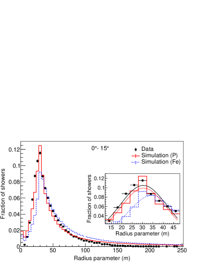
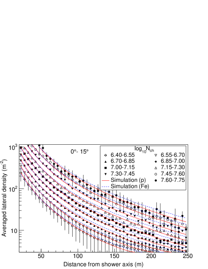
Figure 6: Left: Comparison of normalized distributions of radius parameter obtained from the measurements (points) and simulations (thick-solid line: protons and thin-dashed line: iron nuclei) for showers with reconstructed sizes $\log_{10}N_{\mathrm{ch}}>6.40$ and reconstructed zenith angles between $0^{\circ}$ and $15^{\circ}$. The inset shows Gaussian fits (thin lines) to the distributions around the maximum. Right: Comparison of the averaged lateral distributions between measurements and simulations. The measurements (symbols) are the same as shown in Figure 2 right panel and the lines (solid: protons and dashed: iron nuclei) are the simulation results for the same shower size bin.

Figure 5 shows the total acceptance of the array for primary protons and iron nuclei as a function of the true energy. The detector acceptance $A_{\mathrm{acc}}$ is defined as the total effective area of the array multiplied by the effective viewing angle, and it is calculated as,

$$A_{\mathrm{acc}}(E_{\mathrm{T}})=\int^{\Omega_{c}}_{0}A_{\mathrm{proj}}(\theta)\epsilon_{\mathrm{tot}}(E_{\mathrm{T}},\theta,\phi)d\Omega,$$ (3)

where $d\Omega=\sin\theta~{}d\theta~{}d\phi$ is the solid angle subtended by an element of opening angle between $\theta$ and $\theta+d\theta$ and an azimuthal width of $d\phi$. $\Omega_{c}$ is the maximum solid angle corresponding to the zenith angle cut of $\theta_{c}=35^{\circ}$, $A_{\mathrm{proj}}=\pi~{}R_{\mathrm{c}}^{2}~{}\cos\theta$ is the projected geometrical area of the array at an inclination $\theta$ with $R_{\mathrm{c}}=150$ m representing the fiducial radial cut applied in the analysis, and the total efficiency, $\epsilon_{\mathrm{tot}}$, is given as a function of $(E_{\mathrm{T}},\theta,\phi)$. Assuming azimuthal symmetry of $\epsilon_{\mathrm{t}}$, the integral in Equation 3 is discretized in zenith angle bins and can be rewritten as,

$$A_{\mathrm{acc}}(E_{\mathrm{T}})=\frac{\pi^{2}R^{2}_{\mathrm{c}}}{2}\sum\limits_{k=1}^{n_{\theta}}\epsilon_{\mathrm{t}}(E_{\mathrm{T}},\theta_{\mathrm{k}})\\ \left(\cos 2\theta_{\mathrm{k}}-\cos 2\theta_{\mathrm{k+1}}\right),$$ (4)

where $k$ denotes the zenith angle bins, $n_{\theta}=4$ is the number of zenith angle bins considered, and $\theta_{\mathrm{k}}$ and $\theta_{\mathrm{k+1}}$ represent the low-bin and high-bin edges of each zenith angle bin respectively.

5 Comparison between simulations and measurements

In Figure 6 (left panel), the normalized distribution of radius parameters for the simulated showers with reconstructed sizes $\log_{10}N_{\mathrm{ch}}>6.40$ is compared with the measurements for the zenith angle range of $0^{\circ}-15^{\circ}$. The points in the figure represent the measurements and they are the same as shown in Figure 2 (left panel). The distribution for iron nuclei (thick-dashed line) shows a systematic shift towards larger $r_{\mathrm{M}}$ with respect to the proton showers (thick-solid line) which is expected due to the difference in the shower development between proton and iron primaries. Showers induced by iron nuclei are generated higher up in the atmosphere, resulting in a larger spread (which implies larger $r_{\mathrm{M}}$ values) on the ground, relative to the proton showers. Although both the simulated distributions follow a similar shape as the measured distribution, they are not in full agreement with the data. But, overall, the proton distribution seems to be relatively closer to the data. The inset shows a closer view for the region around the maximum between 12 and 48 m. The lines represent fits to the distributions using a Gaussian function. The Gaussian peaks for the simulated distributions obtained from the fits are $(30.51\pm 0.01)$ m for the proton distribution and $(34.38\pm 0.02)$ m for the iron distribution. The value for the proton distribution is found to be quite close to the peak value of $(30.33\pm 0.13)$ m obtained for the data.

Figure 6 (right panel) shows a comparison of the averaged lateral distribution between simulations and measurements for a reconstructed shower size in the range of $6.40<\log_{10}N_{\mathrm{ch}}<7.75$. The measurements (points) are the same as already shown in Figure 2 (right panel). The iron distributions (dashed lines) are found to be slightly flatter than the proton distributions (solid lines), which is expected due to the larger $r_{\mathrm{M}}$ values for iron showers as explained above. Although both the simulated proton and iron distributions are consistent with the data within the experimental uncertainties, the proton distributions seem to agree better as the iron distributions tend to show some systematic deviation from the measurements above a distance of $\sim 70$ m from the shower axis. A $\chi^{2}$ test of the comparison between the simulations and the measurements gives reduced $\chi^{2}$ values within the range of $\sim 1.15-1.26$ for protons and $\sim 1.33-1.86$ for the case of iron nuclei. The better agreement of the measurements with the proton distributions is expected because the air shower particles measured by LORA are mostly dominated by electrons rather than muons, which makes the measurements biased towards protons.

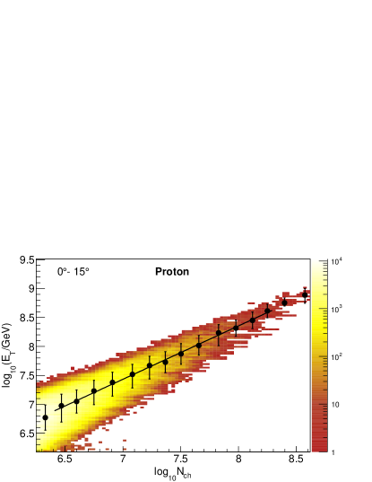
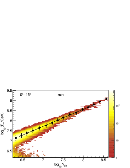
Figure 7: Two-dimensional histogram for the reconstructed shower size $N_{\mathrm{ch}}$ and true energy $E_{\mathrm{T}}$, obtained from simulations for showers induced by protons (left) and iron nuclei (right) for a zenith angle bin of $0^{\circ}-15^{\circ}$. The distributions are weighted to an energy spectrum of index -3. Each point represents the peak in the true energy distribution for a $\log_{10}N_{\mathrm{ch}}$ bin width of 0.15 (see Section 6 for details). The lines represent fits to the points using Equation 6 in the range of $6.4<\mathrm{log}_{10}N_{\mathrm{ch}}<8.3$ for protons and $6.3<\mathrm{log}_{10}N_{\mathrm{ch}}<8.3$ for iron nuclei. The fit parameters are listed in Table 2.

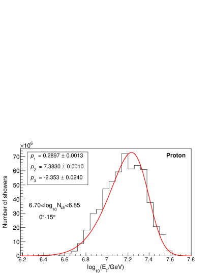
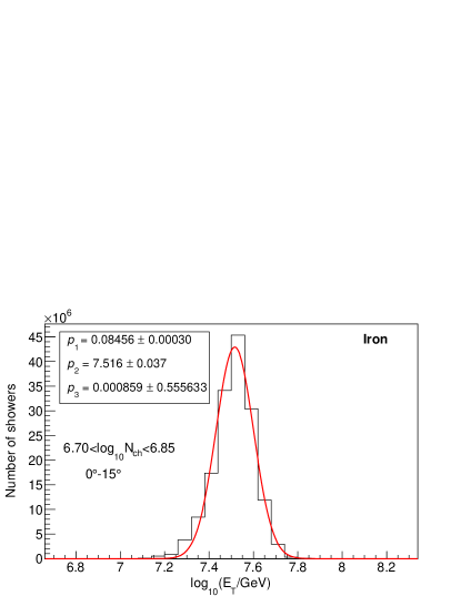
Figure 8: True energy distribution for the reconstructed size bin of $6.70<\mathrm{log}_{10}N_{\mathrm{ch}}<6.85$ for protons (left panel) and iron nuclei (right panel) for the zenith range $0^{\circ}-15^{\circ}$. The distributions are weighted to an energy spectrum of index -3. The lines represent fits using a skewed Gaussian function given by Equation 5 which involves four parameters (see Section 6 for details). Main fit parameters $(p_{1},p_{2},p_{3})$ are shown.

Table 2: Fit parameters for showers induced by protons and iron nuclei obtained by fitting Equation 6 to the size-energy profile plots for different zenith angle bins between $0^{\circ}$ and $35^{\circ}$. A slope $\gamma_{\mathrm{s}}=-3$ of the differential cosmic-ray energy spectrum has been adopted in the simulations.

Zenith angle	Protons			Iron nuclei
$\theta$	a	b		a	b
$0^{\circ}-15^{\circ}$	$0.980\pm 0.683$	$0.922\pm 0.089$		$1.747\pm 0.361$	$0.853\pm 0.048$
$15^{\circ}-24^{\circ}$	$1.234\pm 0.766$	$0.898\pm 0.099$		$1.801\pm 0.370$	$0.858\pm 0.049$
$24^{\circ}-30^{\circ}$	$1.315\pm 0.815$	$0.901\pm 0.101$		$1.726\pm 0.319$	$0.885\pm 0.041$
$30^{\circ}-35^{\circ}$	$1.667\pm 0.692$	$0.873\pm 0.091$		$1.982\pm 0.366$	$0.866\pm 0.048$

6 Energy calibration

The measured shower size can be converted into the energy of the primary particle using a conversion relation obtained from simulations. Simulated showers are stored in a two dimensional log-log histogram in reconstructed size and true energy. Such a histogram is shown in Figure 7 for showers induced by protons (left panel) and iron nuclei (right panel) for the zenith angle range of $0^{\circ}-15^{\circ}$. The color profile represents the weight of the distribution. The distribution is broader for proton showers, which is mainly due to the large intrinsic fluctuations of proton showers. From simulations, the fluctuations in the true shower size for proton showers within the $0^{\circ}-15^{\circ}$ zenith angle bin are found to be $\sim(30-45)\%$ while the uncertainty due to the reconstruction is in the range of $\sim(12-19)\%$ for the energy region of our interest. For iron induced showers, the intrinsic size fluctuation is only $\sim(17-22)\%$, while the reconstruction accuracy remains almost the same as that of the proton induced showers. Another major difference is that for the same reconstructed shower size, iron showers have higher energies than the protons. This is related to the shallower penetration depth of iron induced showers in the atmosphere, which leads to an increased attenuation of electrons before they can reach the ground.

The distributions in Figure 7 are binned in $N_{\mathrm{ch}}$, taking a logarithmic bin size of $0.15$, and profile plots of the true energy as function of $N_{\mathrm{ch}}$ are generated. The profile plots are represented by the solid points in Figure 7. Each point in the plots represents the peak of the energy distribution for each size bin, and the uncertainty on each point corresponds to the spread of the energy distribution which is described in detail in the following. Figure 8 shows the energy distribution for the bin slice of $\log_{10}N_{\mathrm{ch}}=6.70-6.85$ for both, showers induced by protons (left panel) and iron nuclei (right panel). The distribution for protons is not symmetric about its mean and is found to be more extended to lower energies. This can be understood as more contamination from low-energy showers in a given size bin than from higher energies which is caused by the larger intrinsic fluctuations of low-energy showers. The level of contamination depends on the assumed slope of the primary cosmic-ray spectrum in the simulation. The peaks of the distributions are obtained by fitting with a skewed Gaussian function. The skewed Gaussian distribution function used in the present analysis is given by,

$$f(x)=\frac{p_{0}}{p_{1}}\exp\left(-\frac{\left(x-p_{2}\right)^{2}}{2p_{1}^{2}}\right)\left[1+\mathrm{erf}\left(\frac{p_{3}(x-p_{2})}{\sqrt{2p_{1}^{2}}}\right)\right],$$ (5)

where $x=\log_{10}\left(E_{\mathrm{T}}/\mathrm{GeV}\right)$, $p_{0}$ is the normalisation constant, $p_{1}$ and $p_{2}$ represent measures of the spread and the position of the distribution respectively, and $p_{3}$ is the skewness parameter of the distribution function.

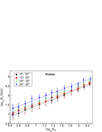
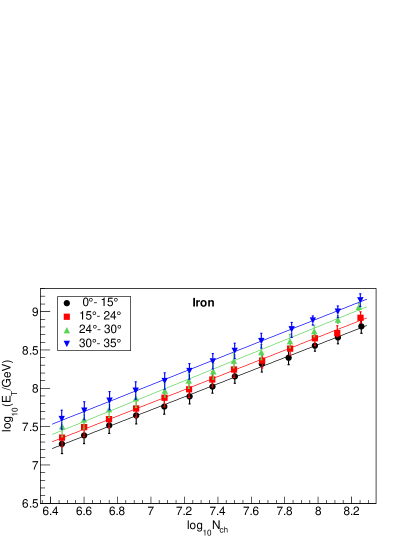
Figure 9: Reconstructed size ($N_{\mathrm{ch}}$) and true energy ($E_{\mathrm{T}}$) relation for proton (left) and iron (right) showers for all zenith angle ranges up to $35^{\circ}$.

The lines in Figure 8 represent the fitted functions. The important fit parameters $(p_{1},p_{2},p_{3})$ are also shown. For the distribution of iron-induced showers, it can be noticed that the value of $p_{3}$ is close to zero, indicating that the distribution closely resembles a normal Gaussian distribution. The uncertainties in the profile plots shown in Figure 7 are obtained by taking the difference between the energies corresponding to the full width at half maximum (FWHM) and the peak energy of the energy distribution for each size bin. The uncertainties obtained are asymmetric for the proton distribution while for iron induced showers, they are almost symmetric. The $N_{\mathrm{ch}}$ values of the profile plots shown in Figure 7 are calculated as the weighted mean of the size distribution within each size bin. These size values are found to be slightly smaller than the bin centers.

To obtain the size-energy relation, each profile plot is fitted using the following function,

$$\centering\log_{10}E_{\mathrm{T}}=a+b\log_{10}N_{\mathrm{ch}}\@add@centering$$ (6)

where $E_{\mathrm{T}}$ denotes the true energy, and $a$ and $b$ are the fit parameters. The fit is performed only in the size region where a reliable fit of the true energy distribution, as shown in Figure 8, could be performed. This corresponds to a size region of $\log_{10}N_{\mathrm{ch}}=6.4-8.3$ for both the type of particles. The profile plots as well as the fitted functions for all the zenith angle ranges are shown in Figure 9 for protons (left panel) and iron nuclei (right panel).

From these figures, it can be noticed that for the same shower size, primary energies at larger zenith angles are larger than at smaller angles. In other words, it requires a higher energy at larger zenith angles to generate the same number of particles on the ground as at lower zenith angles. This is due to higher attenuation of air shower particles at larger zenith angles as the showers pass through a longer column depth of air in the atmosphere. The values of the $a$ and $b$ parameters obtained from the fits for the four zenith angle ranges are listed in Table 2. Using these values, for any simulated or measured shower for which the reconstructed arrival direction and the reconstructed size are known, the primary cosmic-ray energy can be reconstructed using the relation

$$\centering\log_{10}E_{\mathrm{R}}=a+b\log_{10}N_{\mathrm{ch}},\@add@centering$$ (7)

where $E_{\mathrm{R}}$ denotes the reconstructed energy.

7 Energy resolution and systematic uncertainties

In this section, we present details about the accuracy of the reconstructed energies and the uncertainties that have to be considered for the reconstruction of the cosmic-ray intensity. The accuracy depends on the variation of the true shower size caused by the intrinsic shower-to-shower fluctuations in the atmosphere and also on the accuracy in the reconstruction of the shower size.

7.1 Energy resolution

For each size bin in the $E_{\mathrm{T}}-N_{\mathrm{ch}}$ profile plot, reconstructed energies $(E_{\mathrm{R}})$ are obtained for every simulated shower, and a distribution of the differences between the true energies and the reconstructed energies $(E_{\mathrm{T}}-E_{\mathrm{R}})$ is generated. The distribution obtained is similar to the one shown in Figure 8, except for a shift in the peak position to the left by an interval equal to the value of the reconstructed energy. The peak position and the spread of these distributions are obtained correspondingly. The peak represents the systematic uncertainty due to energy calibration, while the spread corresponds to the energy resolution. Their values expressed as fraction of the reconstructed energies are shown in Figure 10 as function of the shower size for the zenith angle range of $\theta=0^{\circ}-15^{\circ}$. The resolution is in the range of $\sim 28\%-48\%$ for proton induced showers and $\sim 12\%-32\%$ for showers induced by iron nuclei. The systematics are within 12% for protons and within 8% for iron nuclei. At $\theta=30^{\circ}-35^{\circ}$, the uncertainty in energy for protons increases to the range of $\sim 37\%-65\%$ in resolution and to $\sim 20\%$ in systematics. For iron nuclei, the uncertainty remains almost the same up to $\theta=35^{\circ}$.

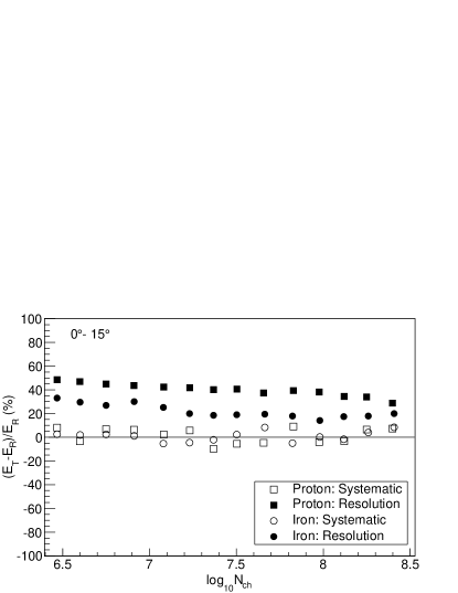
Figure 10: Accuracy in the reconstructed energies ($E_{\mathrm{R}}$) for showers induced by protons (squares) and iron nuclei (circles) as a function of the reconstructed size $N_{\mathrm{ch}}$ for the zenith angle bin of $0^{\circ}-15^{\circ}$. The filled points represent the energy resolution and the the empty points are the systematic uncertainties resulting from the energy calibration. See Section 7.1 for details.

7.2 Systematic uncertainty in energy

The systematic uncertainty in energy shown in Figure 10 is associated with the energy calibration performed using Equation 7. Other main sources of systematic uncertainty in energy include the assumed slope of the primary cosmic-ray spectrum in the CORSIKA simulation, the VEM peak obtained from the detector simulation and the hadronic interaction models. Thus, the calibration parameters, listed in Table 2, also depend on the choice of simulation parameters.

A part of the systematic uncertainties are obtained by changing the values of the slope and the VEM peak in the simulations within reasonable limits, and by comparing the newly reconstructed energies with the energies obtained using the fixed parameters given in Table 2. For the slope of the energy spectrum, simulated showers with an original slope $\gamma_{\mathrm{s}}=-2$ are weighted to generate distributions for $\gamma_{\mathrm{s}}=-2.5$ and $\gamma_{\mathrm{s}}=-3.5$. Then, following the same procedure as described in Section 6, energy calibrations are performed separately for the two different slopes and calibration parameters are obtained. The differences between the energies reconstructed with the new parameters and the ones reconstructed using the parameters given in Table 2 gives the systematic uncertainty due to the spectral slope. The uncertainties are found to be within $(+6\%,-9\%)$ for protons and within $\pm 2\%$ for iron nuclei.

From the detector simulation, it has been observed that adding noise to the deposited energy in the detector at the level of $1$ MeV (see Section 4.2) leads to around $10\%$ positive shift in the value of the most probable energy deposition $E_{\mathrm{VEM}}$ in the detector for vertical incident muons. The 10% increase in $E_{\mathrm{VEM}}$ will lead to a decrease in the shower size and subsequently to an increase in the reconstructed energy by $\sim 10\%$. The average systematic shift in the reconstructed energy due to this uncertainty in VEM calibration is obtained to be $\sim+10\%$ for showers induced by either protons or iron nuclei. The different systematic uncertainties obtained are shown in Figure 11 as a function of the reconstructed energy for showers induced by protons (left panel) and iron nuclei (right panel). For proton showers, the total systematic uncertainty, obtained by adding the individual systematic components in quadrature, is found to be within $\sim(+20\%,-10\%)$ and for iron showers, the total systematic is within $(+10\%,-5\%)$. At larger zenith angles, the total systematic for protons increases slightly, reaching $\sim(+22\%,-15\%)$ at $\theta=30^{\circ}-35^{\circ}$, while for iron nuclei, the uncertainty remains almost unchanged.

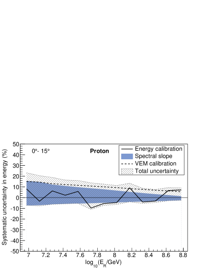
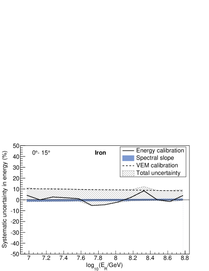
Figure 11: Systematic uncertainties in the reconstructed energy $(E_{\mathrm{R}})$ for showers induced by protons (left panel) and iron nuclei (right) for the zenith angle bin of $0^{\circ}-15^{\circ}$ as a function of $E_{\mathrm{R}}$. The systematic uncertainties due to the energy calibration (thick solid lines) are the same as shown in Figure 10 but plotted as function of $E_{\mathrm{R}}$. They are calculated using the parameters set given in Table 2 for $\gamma_{\mathrm{s}}=-3$. The blue band represents the uncertainty resulting from changing the spectral slope from $-2.5$ to $-3.5$. The dashed line is due to the uncertainty involved in the VEM calibration and the shaded-striped region is the total uncertainty.

7.3 Systematic uncertainty in intensity

Any systematic uncertainty in energy results in a systematic shift in the reconstructed cosmic-ray flux intensity. To estimate the systematic uncertainty in intensity due to the energy calibration, the reconstructed energies are determined using Equation 7 for all simulated showers with $\gamma_{\mathrm{s}}=-3$ that pass through all selection and quality cuts as listed in Table 1. The distribution of the reconstructed energies is compared to the distribution of the true energies, and the systematic uncertainty in intensity is calculated as $(I_{\mathrm{T}}-I_{\mathrm{R}})/I_{\mathrm{R}}$ for each energy bin, where $I_{\mathrm{T}}$ and $I_{\mathrm{R}}$ represent the number of showers per bin in the true and reconstructed energy distributions respectively.

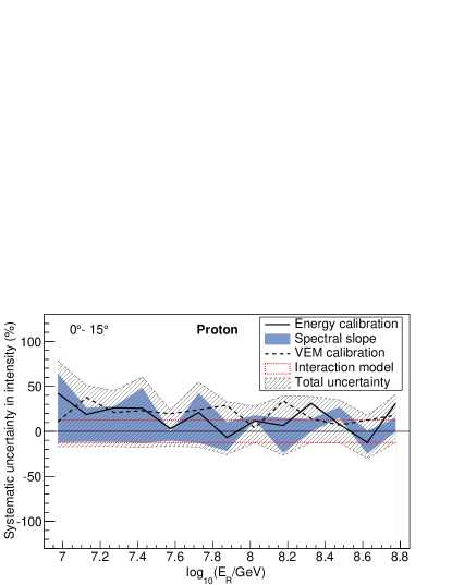
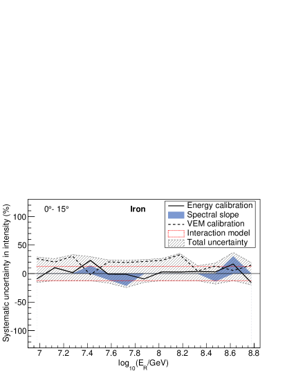
Figure 12: Systematic uncertainties in intensity obtained from simulations of showers induced by protons (left panel) and iron nuclei (right panel) for the zenith angle bin of $0^{\circ}-15^{\circ}$. All lines/bands (except the dotted band) have the same representation as in Figure 11. The dotted band represents the uncertainty expected due to the hadronic interaction model which is taken as $12.5\%$.

For the systematic effect due to the uncertainties in the spectral slope and the VEM calibration, the energy calibration determined in their respective cases are applied to the simulated showers for $\gamma_{\mathrm{s}}=-3$ and the distributions of the newly reconstructed energies are compared with the old distribution obtained using the parameters given in Table 2.

Figure 12 shows the different systematic uncertainties in intensity that have been obtained for protons (left panel) and iron nuclei (right panel). The thick solid line represents the systematic uncertainty due to the energy calibration, the blue band represents the contribution due to the spectral slope, the dashed line is the VEM contribution, and the shaded-striped region represents the total systematic uncertainty. For energies above $\log_{10}(E_{\mathrm{R}}/\mathrm{GeV})\sim 7.2$, the systematic uncertainty due to the energy calibration is found to be within $\sim(+30\%,-10\%)$ for proton showers and within $\sim(+20\%,-10\%)$ for showers induced by iron nuclei. The systematic uncertainty due to the spectral slope is within $\sim(+40\%,-15\%)$ for protons, and within $\sim(+12\%,-18\%)$ for iron nuclei except at $\log_{10}(E/\mathrm{GeV})\sim 8.6$ where the uncertainty reaches $\sim 30\%$. The systematic uncertainty associated with the VEM calibration is found to be within $+30\%$ for both types of nuclei. A contribution of $12.5\%$ due to the uncertainty in the hadronic interaction model [30, 31] is also included in Figure 12. For protons, the total systematic uncertainty above $\log_{10}(E_{\mathrm{R}}/\mathrm{GeV})\sim 7.2$ is within $\sim(+60\%,-25\%)$, and for iron nuclei, the total uncertainty is within $\sim(+38\%,-20\%)$.

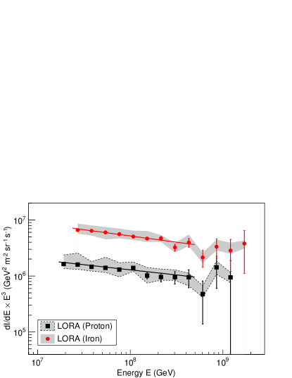
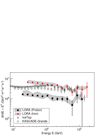
Figure 13: Left: All-particle cosmic-ray energy spectrum measured with LORA, assuming that cosmic rays are only protons (squares) and iron nuclei (filled circles). The error bars represent statistical uncertainties and the shaded areas represent systematic uncertainties. The lines represent single power law fits to the measurements, excluding the highest three energy bins. Right: LORA measurements compared to the all-particle energy spectrum from IceTop (crosses) and KASCADE-Grande (empty circles) measurements.

8 Measured cosmic-ray energy spectrum

For all high-quality LORA data, reconstructed energies are determined on shower-by-shower basis, and a distribution of reconstructed energies is built taking a logarithmic bin size of 0.15. From the distribution, the differential cosmic-ray spectrum $(dI/dE)$ is obtained by folding in the total acceptance of the LORA array $A_{\mathrm{acc}}$ (Figure 5) and the total observation time $T_{\mathrm{obs}}$ as follows,

$$\centering\left(\frac{dI}{dE}\right)_{i}=\left(\frac{\Delta n}{\Delta E}\right)_{i}\times\frac{1}{A_{\mathrm{acc}}T_{\mathrm{obs}}}\@add@centering$$ (8)

where the subscript $i$ denotes the $i^{\mathrm{th}}$ energy bin and $\Delta n$ is the number of showers in an energy bin of width $\Delta E$. For constructing the spectrum, only the energy region that has a total (trigger and reconstruction) efficiency greater than $98\%$ is used. This corresponds to an energy of $1.9\times 10^{7}$ GeV for protons and $2.7\times 10^{7}$ GeV for iron nuclei (see Figure 4).

Figure 13 (left panel) shows the reconstructed energy spectrum multiplied by $E^{3}$, assuming that cosmic rays are only protons or iron nuclei. The spectrum is given in the energy range of $(1.9\times 10^{7}-1.2\times 10^{9})$ GeV for protons, and in the range of $(2.7\times 10^{7}-1.7\times 10^{9})$ GeV for iron nuclei. The measured values along with the uncertainties are listed in Table 3. The measured spectra cannot be described by single power laws over the full energy range because of the structures present in the spectra, particularly the dip at $\sim 6\times 10^{8}$ GeV. A power law fit to the measured spectra data below $5\times 10^{8}$ GeV gives spectral index values of $\gamma_{\mathrm{P}}=-3.18\pm 0.13$ for protons and $\gamma_{\mathrm{Fe}}=-3.22\pm 0.08$ for iron nuclei.

In Figure 13 (right panel), our measured spectra are compared with the all-particle spectra measured with the IceTop [29] and KASCADE-Grande [30] experiments. Both their spectra lie between our reconstructed spectra, which is expected in the case of a mixed cosmic-ray composition. They are close to our proton spectrum at $\sim 2\times 10^{7}$ GeV, and become closer to our iron spectrum as the energy increases. This might be an indication of a change in the mass composition of cosmic rays in the energy region between $10^{7}$ and $10^{9}$ GeV, which is expected as due to a transition from a Galactic to an extragalactic origin of cosmic rays.

9 Conclusion and outlook

We have conducted a detailed energy reconstruction study for the extensive air showers measured with the LORA particle detector array. Important parameters such as the energy resolution of the array and the systematic uncertainty of the reconstructed energy have been obtained. The energy resolution is found to be in the range of $\sim 28-48\%$ for showers induced by protons and $\sim 12-32\%$ for iron nuclei. The total systematic uncertainty of the reconstructed energy is within $\sim(+20\%,-10\%)$ for protons and within $\sim(+10\%,-5\%)$ for iron nuclei. Applying the reconstruction method to the measured data, the all-particle cosmic-ray energy spectrum has been obtained, assuming that cosmic rays are only constituted of protons or iron nuclei for energies above $\sim 10^{16}$ eV with a systematic uncertainty in intensity of $\sim 20-60\%$. Our future effort will concentrate on combining the energy measurement of LORA with the composition measurement from the LOFAR radio antennas to determine an all-particle energy spectrum, taking into account the actual cosmic-ray composition.

Especially the primary energy determined using the energy calibration given here is being used in the reconstruction of air shower properties with the radio data from LOFAR. Calculation of energy calibration parameters for higher zenith angles above $\sim 40^{\circ}$ is underway. This is particularly important for the LOFAR radio measurements where a significant fraction of showers have been observed at larger zenith angles. At present, the small size of the LORA array effectively limits the effective area of LOFAR. Efforts are ongoing to expand the size of the array to exploit the full potential of LOFAR.

Table 3: Values of the measured cosmic-ray spectrum, assuming that cosmic rays are only protons or iron nuclei. The energies are given in GeV and the intensities along with the statistical and the systematic uncertainties are given in units of 1/(m² sr s GeV).

Energy	Intensity $\pm$ stat. $\pm$ sys. uncertainties [1/(m2 sr s GeV)]
(GeV)	Protons	Iron nuclei
$1.91\times 10^{7}$	$(2.34\pm 0.02$ ${}^{+1.05}_{-0.39})\times 10^{-16}$	$-$
$2.70\times 10^{7}$	$(8.13\pm 0.14$ ${}^{+4.91}_{-1.45})\times 10^{-17}$	$(3.35\pm 0.02$ ${}^{+0.99}_{-0.42})\times 10^{-16}$
$3.81\times 10^{7}$	$(2.63\pm 0.06$ ${}^{+0.61}_{-0.42})\times 10^{-17}$	$(1.15\pm 0.01$ ${}^{+0.27}_{-0.19})\times 10^{-16}$
$5.39\times 10^{7}$	$(8.97\pm 0.33$ ${}^{+4.48}_{-1.58})\times 10^{-18}$	$(3.84\pm 0.06$ ${}^{+0.88}_{-0.94})\times 10^{-17}$
$7.61\times 10^{7}$	$(2.94\pm 0.15$ ${}^{+0.97}_{-0.76})\times 10^{-18}$	$(1.26\pm 0.03$ ${}^{+0.31}_{-0.19})\times 10^{-17}$
$1.07\times 10^{8}$	$(1.11\pm 0.08$ ${}^{+0.31}_{-0.14})\times 10^{-18}$	$(4.08\pm 0.15$ ${}^{+1.07}_{-0.51})\times 10^{-18}$
$1.52\times 10^{8}$	$(2.91\pm 0.35$ ${}^{+1.15}_{-0.77})\times 10^{-19}$	$(1.32\pm 0.07$ ${}^{+0.47}_{-0.16})\times 10^{-18}$
$2.14\times 10^{8}$	$(9.71\pm 1.71$ ${}^{+3.77}_{-1.21})\times 10^{-20}$	$(4.75\pm 0.38$ ${}^{+0.65}_{-0.59})\times 10^{-19}$
$3.03\times 10^{8}$	$(3.43\pm 0.86$ ${}^{+1.20}_{-0.43})\times 10^{-20}$	$(1.16\pm 0.15$ ${}^{+0.21}_{-0.21})\times 10^{-19}$
$4.28\times 10^{8}$	$(1.21\pm 0.43$ ${}^{+0.21}_{-0.36})\times 10^{-20}$	$(5.06\pm 0.88$ ${}^{+1.87}_{-0.63})\times 10^{-20}$
$6.04\times 10^{8}$	$(2.15\pm 1.52$ ${}^{+0.87}_{-0.27})\times 10^{-21}$	$(9.72\pm 3.24$ ${}^{+1.87}_{-1.95})\times 10^{-21}$
$8.54\times 10^{8}$	$(2.28\pm 1.32$ ${}^{+0.66}_{-0.56})\times 10^{-21}$	$(5.34\pm 2.02$ ${}^{+1.74}_{-0.66})\times 10^{-21}$
$1.20\times 10^{9}$	$(5.38\pm 5.38$ ${}^{+1.18}_{-1.05})\times 10^{-22}$	$(1.62\pm 0.94$ ${}^{+0.59}_{-0.20})\times 10^{-21}$
$1.70\times 10^{9}$	$-$	$(7.66\pm 5.42$ ${}^{+0.97}_{-1.33})\times 10^{-22}$

References

- [1] Nagano, M., Watson, A. A, 2000, Rev. Mod. Phys., 72, 689
- [2] Blümer, J., Engel, R., Hörandel, J, 2009, Prog. Part. Nucl. Phys. 63, 293
- [3] Hörandel, J. R., 2008, Rev. Mod. Astron. 20, 203
- [4] Hörandel, J. R., 2006, JPhCS, 47, 41
- [5] Thoudam & Hörandel, J. R., 2014, A&A, 567, A33
- [6] Hörandel, J. R., 2004, APh, 21, 241
- [7] Hillas, A.M., J. Phys. G: Nucl. Part. Phys., 2005, 31, R95
- [8] Berezhko, E. G., 2009, ApJ, 698, L138
- [9] Hörandel, J. R., 2008, AdSpR, 2008, 41, 442
- [10] Blasi, P., 2013, A&ARv, 21, 70
- [11] Blasi, P., 2014, BrJPh, 44, 426
- [12] van Haarlem, M., 2013, A&A, 556, A2
- [13] Schellart, P. et al., 2013, A&A, 560, A98
- [14] Buitink, S. et al., 2014, PRD, 90, 082003
- [15] Nelles, A. et al., 2015, JCAP, 05, 018
- [16] Schellart, P. et al., 2014, JCAP, 10, 014
- [17] Corstanje, A. et al., 2015, APh, 61, 22
- [18] Nelles, A. et al., 2015, APh, 65, 11
- [19] Thoudam, S. et al., 2014, NIMPA, 767, 339
- [20] Kamata, K., & Nishimura, J., 1958, Prog. Theoret. Phys. Suppl., 6, 93
- [21] Greisen, K., 1960, Ann. rev. Nucl. Sci., 10, 63
- [22] Antoni, T., et al. 2001, APh, 14, 245
- [23] Heck, D., 1998, Report FZKA, 6019
- [24] Ostapchenko, S. S., 2011, PRD, 83, 014018.
- [25] Fassò, A., et al., 2005, CERN-2005-10, INFN/TC-05/11, SLAC-R-773
- [26] Nelson, W. R., Hirayama, H. & Rogers, D. W. O, 1985, SLAC-0265
- [27] Kobal, M. et al., 2001, APh, 15, 259
- [28] Agostinelli, S. et al., 2003, NIMPA, 506, 250
- [29] Aartsen, M. G. et al, 2013, PRD, 88, 042004
- [30] Apel, W. D. et al., 2012, APh, 36, 183
- [31] Kang, D. et al., 2013, JPhCS, 409, 012101