Thermodynamics of anisotropic triangular magnets with ferro- and antiferromagnetic exchange

Abstract

We investigate thermodynamic properties like specific heat $c_{V}$ and susceptibility $\chi$ in anisotropic $J_{1}$-$J_{2}$ triangular quantum spin systems ($S=1/2$). As a universal tool we apply the finite temperature Lanczos method (FTLM) based on exact diagonalization of finite clusters with periodic boundary conditions. We use clusters up to $N=28$ sites where the thermodynamic limit behavior is already stably reproduced. As a reference we also present the full diagonalization of a small eight-site cluster. After introducing model and method we discuss our main results on $c_{V}(T)$ and $\chi(T)$. We show the variation of peak position and peak height of these quantities as function of control parameter $J_{2}/J_{1}$. We demonstrate that maximum peak positions and heights in Néel phase and spiral phases are strongly asymmetric, much more than in the square lattice $J_{1}$-$J_{2}$ model. Our results also suggest a tendency to a second side maximum or shoulder formation at lower temperature for certain ranges of the control parameter. We finally explicitly determine the exchange model of the prominent triangular magnets Cs₂CuCl₄ and Cs${}_{\text{2}}$CuBr${}_{\text{4}}$ from our FTLM results.

I Introduction

The 2D triangular $S=1/2$ Heisenberg antiferromagnet (HAF) is the archetypical geometrically frustrated quantum magnet Nakatsuji et al. (2010). Therefore it has been studied in countless investigations. Although there is no pure physical realization due to in-plane symmetry breaking and inter-plane coupling several compounds fall into the wider class of anisotropic triangular magnets where the exchange coupling $J_{2}$ along one of the triangle sides is different from $J_{1}$ along the other two sides Schmidt and Thalmeier (2014). In fact this generalization is not a drawback but opens interesting possibilities. It allows to consider a smooth interpolation between square lattice HAF to isotropic triangular magnet to quasi-1D chain compounds as function of a single tuning parameter $J_{2}/J_{1}$.

Most of the work on this magnetic system was focused on the zero temperature phase diagram as function of anisotropy ratio, spin wave excitations and influence of quantum fluctuations as well as effects of external fields like plateau formation in the magnetization. We will not touch these fundamental topics but refer to Ref. Schmidt and Thalmeier (2014) and references cited therein. Here we will focus on a more practical issue, namely the determination of the exchange constant or at least their anisotropy ratio from thermodynamic quantities of triangular magnets. This can be done by analyzing the experimental temperature dependence of specific heat and magnetic susceptibility where the former is less favorable due to lattice contributions Kini et al. (2006). A simplified but not unambiguous determination of exchange constants is possible by identifying position and height of the maximum in thermodynamic quantities and comparing with theoretical predictions. Further useful tools of diagnosing the exchange model are magnetothermal, e.g. magnetocaloric properties as well as high field magnetization and saturation field. This program has sofar mainly been carried out for frustrated $J_{1}$-$J_{2}$ square lattice magnets Shannon et al. (2004); Schmidt et al. (2007, 2010).

Here we focus on the numerical investigation of much less studied finite temperature properties of anisotropic triangular quantum spin systems. Previous investigations used variants of Monte Carlo methods for the quantum case Kawamura and Miyashita (1984); Suzuki and Matsubara (1998); Kulagin et al. (2013), also for the classical case Melchy and Zhitomirsky (2009); Tamura and Tanaka (2013) or analytical methods for the low temperature regime Mezio et al. (2012) and high temperature series expansion Zheng et al. (2005). In the present work we use the finite temperature Lanczos method (FTLM) based on the exact diagonalization (ED) of finite lattice tiles for this purpose. The method is based on evaluating the partition function by averaging over random starting vectors in the ED procedure. Using periodic boundary conditions and discrete symmetries we can go up to largest cluster size of $N=28$ sites for thermodynamic averages. We also consider smaller clusters of size $N=16,20,24$ by FTLM. Furthermore we present the full analytical solution of the spectrum for the smallest $N=8$ cluster as a reference point. However, we note that unlike zero temperature ED results for finite clusters the FTL method cannot be used for finite size scaling analysis of thermodynamic quantities. Nonetheless in the special case of the 1D chain system ($J_{1}=0$) we can compare to exact results which are in excellent agreement with the $N=28$ cluster results. This indicates that our FTLM results are trustworthy to use as a representation for the thermodynamic limit.

Our main emphasis is the calculation of peak position $T_{\text{max}}$ and height $C_{V}(T_{\text{max}})$ and $\chi(T_{\text{max}})$ in the temperature dependence of specific heat and susceptibility, respectively. We investigate its systematic variation with anisotropy control parameter $J_{2}/J_{1}$ or $\phi=\tan^{-1}(J_{2}/J_{1})$, in particular when it is tuned between the simple special cases mentioned above. This information is of great importance for the analysis of thermodynamic data of triangular magnets. The $T_{\text{max}}(\phi)$ dependence turns out to be considerably more asymmetric than for the related square lattice model Shannon et al. (2004). We show that in certain ranges of the control parameter an indication of second maximum or shoulder in these quantities appears. Furthermore as an example we discuss the analysis of the full temperature dependence of $\chi(T)$ for the most prominent triangular quantum spin systems Cs₂CuCl₄ and the isostructural Cs${}_{\text{2}}$CuBr${}_{\text{4}}$ using FTLM results. We demonstrate that the derived exchange model is in excellent agreement with the one obtained from direct spectroscopic methods like inelastic neutron scattering (INS, Cs${}_{\text{2}}$CuCl${}_{\text{4}}$ only) spin wave results and electron spin resonance (ESR) experiments, both in high fields.

In Sec. II we define the model and its parametrization. The reference of the full solution for the eight-site cluster is discussed in Sec. III. The FTL method and its technical implementation are discussed to some extent in Sec. IV. Our main results on specific heat and susceptibility are presented in Secs. V and VI, respectively and the explicit comparison to Cs₂CuCl₄ and Cs₂CuBr₄ is discussed in Sec. VII. Finally Sec. VIII gives the conclusion and outlook.

II Anisotropic triangular exchange model and its parametrization

Figure 1: Schematic view of anisotropic triangular exchange models. For $J_{1}=0$ ($\phi=\pm\pi/2$) this reduces to 1D $J_{2}$-spin chains ($\parallel$), for $J_{2}=0$ ($\phi=0$) to the square lattice $J_{1}$- HAF ($\square$) and for $J_{1}=J_{2}$ ($\phi=\pi/4$) to the isotropic triangular system ($\triangle$).

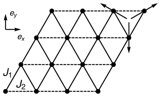
The anisotropic $J_{1}-J_{2}$ exchange model on the triangular lattice (Fig. 1) is given by

$${\cal H}=\sum_{\left\langle ij\right\rangle}J_{ij}{\bf S}_{i}\cdot{\bf S}_{j}$$ (1)

with

$$J_{ij}=\left\{\begin{array}[]{l@{\mbox{ if }}l}J_{1}&{\bf R}_{j}={\bf R}_{i}\pm\frac{1}{2}\left({\bf e}_{x}\pm\sqrt{3}{\bf e}_{y}\right)\\ J_{2}&{\bf R}_{j}={\bf R}_{i}\pm{\bf e}_{x}\end{array}\right.,$$ (2)

where ${\bf e}_{x},{\bf e}_{y}$ are unit vectors along cartesian directions. Figure 1 may also be interpreted as tilted square lattice model with one diagonal $J_{2}$ bond cut out Schmidt and Thalmeier (2014). For the anisotropic triangular-lattice model, different parametrizations of the exchange energies are customary. As introduced in Ref. Shannon et al. (2004) and used subsequently we prefer the polar representation defined by

$$J_{1}=J_{\text{c}}\cos\phi, J_{2}=J_{\text{c}}\sin\phi,$$ (3)

$$J_{\text{c}}=\sqrt{J_{1}^{2}+J_{2}^{2}}, \phi=\tan^{-1}\left(\frac{J_{2}}{J_{1}}\right)$$

where $J_{\text{c}}$ gives the overall energy scale and $\phi$ is the anisotropy control parameter. This parametrization allows for an easy interpolation between important geometrical limiting cases, namely the square-lattice Néel antiferromagnet with $J_{2}=0$ ($\phi=0$), the isotropic $120^{\circ}$ triangular antiferromagnet with $J_{2}=J_{1}$ ($\phi=\pi/4$), the antiferromagnetic chain with $J_{1}=0$ ($\phi=\pi/2$), and their ferromagnetic counterparts. However, there are alternative possibilities in the literature which we briefly mention here for ease of comparison (Fig. 2). Many authors regard the model as an extension to the one-dimensional spin chain, therefore they use the exchange $J_{2}$ along these chains as the overall energy unit and parametrize their results in terms of $\alpha:=J_{1}/J_{2}$ with $J_{1}$ being the interchain coupling. From a square-lattice perspective in turn, the exchange parameter $J_{1}$ appears to be the natural energy unit, and correspondingly $1/\alpha:=J_{2}/J_{1}$ is used as well.

Figure 2: Different exchange parametrizations used for the anisotropic triangular Heisenberg model and their dependence on the anisotropy parameter $\phi$. The left and right branch for $J_{2}/J_{1}$ corresponds to $J_{2}<0$ or $J_{2}>0$, respectively.

Both model parameters $\alpha$ and $1/\alpha$ however are problematic when trying to describe the full phase diagram, in particular the interpolation between the square-lattice antiferromagnet ($\alpha\to\infty$) and the one-dimensional chain ($1/\alpha\to\infty$). To overcome this, the function $f:=J_{2}/(J_{1}+J_{2})=1/(1+\alpha)$ has been introduced in Ref. Zheng et al. (1999), which remains finite in both limits and between these.

However the latter parametrization also does not cover the full phase diagram unambiguously, which is why we have introduced the universal energy scale $J_{\text{c}}$ and the anisotropy angle $\phi$. In the square-lattice case, this has the additional advantage that $J_{\text{c}}$, apart from a global factor $\sqrt{2}$, denotes the magnetocaloric energy scale $J_{\text{mc}}$ as well Shannon et al. (2004). To facilitate the comparison of our results with the literature, Fig. 2 displays the dependence of the quantities introduced here on the anisotropy control parameter $\phi$.

Figure 3: Degree of frustration in per cent in the triangular HAF as function of exchange anisotropy parameter. It vanishes identical in the unfrustrated regime $\phi<0\;(J_{2}<0)$. The dotted lines are the classical phase boundaries Schmidt and Thalmeier (2014).

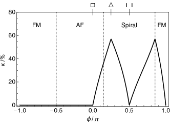
The nearest neighbor (n.n.) HAF model on the triangular lattice is the generic ‘geometrically frustrated’ spin system where the exchange energy of n.n. bonds cannot be minimized simultaneously for all bonds (see upper corner of Fig. 1). It is worthwhile to quantify this intuitive notion of ‘frustration’. A measure for it is the total loss of exchange energy due to frustration relative to the exchange energy without it. For the basic triangular (three-site) plaquette in Fig. 1 the degree of frustration is then given by

$$\kappa(\phi):=1-\frac{E_{\triangle}}{E_{\text{t}}+E_{\text{d}}}$$ (4)

Here $E_{\triangle}$ is the ground state energy of the frustrated triangle. $E_{\text{t}}:=E_{\triangle}(J_{2}=0)$ and $E_{\text{d}}:=E_{\triangle}(J_{1}=0)$ are the ground state energies of its unfrustrated trimer and dimer parts, respectively with

$$E_{\triangle}(\phi):=\min\left(-\frac{3}{4}J_{2},-J_{1}+\frac{1}{4}J_{2},\frac{1}{2}J_{1}+\frac{1}{4}J_{2}\right),$$ (5)

where the minimum is taken from the three different energy eigenvalues of the triangle. Using these expressions in Eq. (4) the degree of frustration (in per cent) in the triangular HAF as function of control parameter is shown in Fig. 3. There the dotted lines indicate the classical boundaries between FM, AF and spiral phases as discussed in Ref. Schmidt and Thalmeier (2014). $\kappa(\phi)$ vanishes identically in the unfrustrated ($J_{2}<0$ or $\phi<0$) case. In the frustrated regime ($J_{2}>0$ or $\phi>0$) it achieves its maximum values of $\kappa=4/7$ corresponding to $57\,\%$ frustration at the isotropic point ($\triangle$) and the Spiral/FM phase boundary while it vanishes for the 1D chain case ($\parallel$) where $J_{1}=0$. We note that the reduction in the ordered ground state moment in the frustrated regime does not directly follow the degree of frustration but is the result of the subtle interplay of the latter with quantum fluctuations Schmidt and Thalmeier (2014).

III Precursor: classical phase diagram and eight-site full solution

Within the finite temperature Lanczos method the thermodynamic quantities will be computed directly using an averaging procedure over the low energy spectrum only. To obtain a better intuition for the triangular Heisenberg model it is useful to calculate also the full spectrum by direct diagonalization of small clusters. We will demonstrate that it develops characteristic signatures at the classical phase boundaries and special symmetry points as function of control parameter using the eight-site cluster.

III.1 Spectrum and classical phase diagram

Figure 4: Sketch of the tile 8:2-2. The edge vectors are ${\bf a}_{1}$ and ${\bf a}_{2}$, the numbers label the individual sites.

As discussed in Ref. Shannon et al. (2004) for the square-lattice model, we can express the spectrum of the triangular eight-site cluster on tile 8:2-2 with periodic boundary conditions as a sum over Hamiltonians on complete graphs. We define

$${\cal H}_{\cal L}^{\text{CG}}:=\sum_{i<j\in{\cal L}}{\bf S}_{i}\cdot{\bf S}_{j}=\frac{1}{2}\left[\left(\sum_{i\in\cal L}{\bf S}_{i}\right)^{2}-\sum_{i\in\cal L}{\bf S}_{i}^{2}\right]$$ (6)

where ${\cal L}$ denotes an ordered list of lattice sites. In our case it has either two elements (a bond), four elements (a square or tetrahedron), or eight elements (a cube). We then can write

$${\cal H}_{8} = J_{1}\left[{\cal H}_{\{1,2,3,4,5,6,7,8\}}^{\text{CG}}-\left({\cal H}_{\{1,3,4,5\}}^{\text{CG}}+{\cal H}_{\{2,6,7,8\}}^{\text{CG}}\right)\right]$$ (7)

$${}+2J_{2}\left[{\cal H}_{\{1,5\}}^{\text{CG}}+{\cal H}_{\{3,4\}}^{\text{CG}}+{\cal H}_{\{2,8\}}^{\text{CG}}+{\cal H}_{\{6,7\}}^{\text{CG}}\right]$$

for the Hamiltonian. The tile and its labelling is illustrated in Fig. 4. From Eq. (7) with $S=1/2$ being the maximum expectation value for each local spin ${\bf S}_{i}$, we get the corresponding list of eigenvalues by hierarchically constructing all possible multiple-spin configurations starting with the basic two-spin singlets and triplets on the pairs $\{1,5\}$, $\{3,4\}$, $\{2,8\}$, and $\{6,7\}$: From all pairs of two-spin states, we can construct the four-spin states with total spin $S=0,1,2$, each possible pair of these four-spin states in turn can be combined to an eight-spin state with total spin $S=0,1,2,3,4$ and spin degeneracy $(2S+1)$ . Because the total spin may be composed in several ways by the spins of sub-clusters there exist additional degeneracies. In this way, we can construct a total of ${N\choose N/2}=70$ states for the eight-site cluster.

Table 1: All energy levels of the eight-site cluster. $S_{1-8}$ is the total cluster spin and the next six columns give the sub-cluster spins. The last column denotes the additional degeneracy of levels on top of the $(2S_{1-8}+1)$-fold spin degeneracy.

$$\begin{array}[]{c|cccccc|c|c}S_{1-8}&S_{1345}&S_{15}&S_{34}&S_{2678}&S_{28}&S_{67}&\text{energy}&\text{deg.}\\ \hline\cr 0&0&0&0&0&0&0&-6J_{2}&\;\;1*\\ 0&0&0&0&0&1&1&-2J_{2}&2\\ 0&0&1&1&0&1&1&2J_{2}&1\\ 0&1&0&1&1&0&1&-2\left(J_{1}+J_{2}\right)&4\\ 0&1&0&1&1&1&1&-2J_{1}&4\\ 0&1&1&1&1&1&1&2J_{2}-2J_{1}&1\\ 0&2&1&1&2&1&1&2J_{2}-6J_{1}&\;\;1*\\ 1&0&0&0&1&0&1&-4J_{2}&4\\ 1&0&0&0&1&1&1&-2J_{2}&2\\ 1&0&1&1&1&0&1&0&4\\ 1&0&1&1&1&1&1&2J_{2}&2\\ 1&1&0&1&1&0&1&-J_{1}-2J_{2}&4\\ 1&1&0&1&1&1&1&-J_{1}&4\\ 1&1&1&1&1&1&1&2J_{2}-J_{1}&1\\ 1&1&0&1&2&1&1&-3J_{1}&4\\ 1&1&1&1&2&1&1&2J_{2}-3J_{1}&2\\ 1&2&1&1&2&1&1&2J_{2}-5J_{1}&1\\ 2&0&0&0&2&1&1&-2J_{2}&2\\ 2&0&1&1&2&1&1&2J_{2}&2\\ 2&1&0&1&1&0&1&J_{1}-2J_{2}&4\\ 2&1&0&1&1&1&1&J_{1}&4\\ 2&1&1&1&1&1&1&J_{1}+2J_{2}&1\\ 2&1&0&1&2&1&1&-J_{1}&4\\ 2&1&1&1&2&1&1&2J_{2}-J_{1}&2\\ 2&2&1&1&2&1&1&2J_{2}-3J_{1}&1\\ 3&1&0&1&2&1&1&2J_{1}&4\\ 3&1&1&1&2&1&1&2\left(J_{1}+J_{2}\right)&2\\ 3&2&1&1&2&1&1&2J_{2}&1\\ 4&2&1&1&2&1&1&2\left(2J_{1}+J_{2}\right)&\;\;1*\\ \end{array}$$

Figure 5: Energy spectrum of the eight-site cluster, classified according to total spin $S$. Solid lines: $S=0$, short-dashed lines: $S=1$, dotted lines: $S=2$, dash-dotted lines: $S=3$, long-dashed lines: $S=4$. The line thickness indicates the degeneracy of the corresponding energy level, see Table 1. The thin vertical lines denote the classical phase boundaries between ferromagnet (FM), Néel antiferromagnet (AF), and spiral structure. The dotted vertical lines denote the three special cases square-lattice Néel antiferromagnet ($J_{1}>0$, $J_{2}=0$), isotropic triangular lattice ($J_{2}\equiv J_{1}>0$), and one-dimensional antiferromagnetic chains ($J_{1}=0$, $J_{2}>0$).

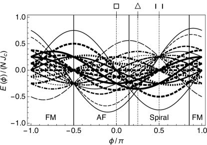
Table 1 displays the complete set of eigenvalues, together with their (additional) degeneracies, total spins, and total spins on the sub-lattices. Of particular interest are those states corresponding to classical ground states (marked by an asterisk in the last column): the columnar antiferromagnet (first state in the table, energy $-6J_{2}$), the Néel antiferromagnet (seventh state, energy $2J_{2}-6J_{1}$), and the ferromagnet (last state, energy $2(2J_{1}+J_{2})$. These three states replace each other as ground states as a function of the anisotropy ratio $\phi$, see Fig. 5. Fig. 5 displays the full spectrum of the tile 8:2-2 as a function of the anisotropy angle. The thicknesses of the lines indicate the degeneracies of the corresponding states as listed in Table 1. Solid lines denote singlet states, the long-dashed line denotes the ferromagnet, for further line types see the figure caption.

We overlay this spectrum to the classical phase diagram of the model discussed in detail in Ref. Schmidt and Thalmeier (2014). The classical FM, AF and spiral phases are separated by the thin vertical lines. The thin dotted lines indicate as special cases the square-lattice Néel antiferromagnet ($\square$, $\phi=0$ or $J_{1}>0$, $J_{2}=0$), isotropic antiferromagnetic triangular lattice ($\triangle$, $\phi=\pi/4$ or $J_{2}\equiv J_{1}>0$) corresponding to the non-collinear $120^{\circ}$ commensurate spiral structure and one-dimensional antiferromagnetic chains ($\parallel$, $\phi=\pi/2$ or $J_{1}=0$, $J_{2}>0$).

Characteristic for the spectrum at these six special points is the high number of degenerate excited states with different total spin. At the borders of the classical ferromagnetic phase also the ground state changes from the fully polarized state to a singlet. However the classical phase boundary between the antiferromagnet and the spiral phase does not correspond to an equivalent change of (in this case nonmagnetic) ground states. This is due to the fact that with our eight-site tile we cannot approximate any incommensurate state at all, therefore the “best” approximation to the “true” ground state remains the Néel state for $1/2\leq J_{2}/J_{1}\leq 3/4$ (equivalent to $0.148\leq\phi/\pi\leq 0.205$), and the columnar antiferromagnetic state for larger values of $J_{2}/J_{1}$.

Similar to the square-lattice case Shannon et al. (2004), we observe level crossings near the classical phase boundary between AF and spiral phase. For the square lattice, we took this as an indication for the appearance of a nonmagnetic phase, coinciding with the suppression of the ordered moment in a region around the classical transition observed within linear spin-wave theory Schmidt and Thalmeier (2014). Qualitatively the same happens here, however this analogy should not be taken too far, because no indication of that kind exists for the classically invisible crossover to one-dimensional chains at $\phi=\pi/2$, which is in reality surrounded by a large nonmagnetic region. And empirically we know that linear spin-wave theory rather underestimates the size of these nonmagnetic regions. At the crossover from the spiral to the ferromagnetic phase for $\phi/\pi\approx 0.852$, a similar type of pattern of level crossings exists. Linear spin-wave theory gives inconsistent results in this case.

III.2 Thermodynamics of the eight-site cluster

Given the eigenvalue $E_{I}$ with degeneracy $d_{I}$ and total spin $S_{I}$ for each state $I$ listed in Table 1, we can easily evaluate the partition function ${\cal Z}=\sum_{I}d_{I}\left(2S_{I}+1\right){\rm e}^{-\beta E_{I}}$ to calculate the magnetic susceptibility $\chi$ and the specific heat $c_{V}$ according to

$$\chi = \frac{\beta J_{\text{c}}}{N}\frac{1}{\cal Z}\sum_{I}d_{I}(2S_{I}+1)\frac{S_{I}(S_{I}+1)}{3}{\rm e}^{-\beta E_{I}},$$ (8)

$$c_{V} = \frac{\beta^{2}}{N}\left[\frac{1}{\cal Z}\sum_{I}d_{I}(2S_{I}+1)E_{I}^{2}{\rm e}^{-\beta E_{I}}\right.$$ (9)

$$\hphantom{\frac{\beta^{2}}{N}}\left.{}-\left(\frac{1}{\cal Z}\sum_{I}d_{I}(2S_{I}+1)E_{I}{\rm e}^{-\beta E_{I}}\right)^{2}\right]$$

where $\beta=1/(k_{\text{B}}T)$ with $k_{\text{B}}$ being the Boltzmann constant. Here and in the following, we express the molar susceptibility in units of $N_{\text{L}}\mu_{0}\left(g\mu_{\text{B}}\right)^{2}J_{\text{c}}^{-1}$, where $N_{\text{L}}$ is the Loschmid constant, $\mu_{0}$ the magnetic permeability constant, $g$ the gyromagnetic ratio, and $\mu_{\text{B}}$ the Bohr magneton. For the dimension of the specific heat $c_{V}$, we use the universal gas constant $R=N_{\text{L}}k_{\text{B}}$.

IV General remarks on finite temperature methods

The finite temperature properties of spin systems can be treated with analytical high temperature expansions Zheng et al. (2005); Oitmaa et al. (2006); Rosner et al. (2003); Nath et al. (2008); Schmidt et al. (2011a) or with the numerical FTL method Jaklič and Prelovšek (2000) which will be employed in this work. As a reference we first discuss briefly the single first order term of the expansion method.

IV.1 High temperature approximation

The high-temperature behavior of the susceptibility $\chi$ and the specific heat $c_{V}$ to quadratic order in $\beta$ is determined by the Curie-Weiss energy $\Theta$ and the magnetocaloric energy scale $J_{\text{mc}}$, which are defined through

$$\Theta := \frac{S(S+1)}{3}\sum_{n}J_{ii+n}=J_{1}+\frac{J_{2}}{2},$$ (10)

$$J_{\text{mc}}^{2} := \frac{1}{2}\sum_{n}J_{ii+n}^{2}=2J_{1}^{2}+J_{2}^{2}.$$ (11)

The sums run over all bonds $n$ connecting an arbitrary but fixed site $i$ with its (not necessarily nearest) neighbors at sites $\{i+n\}$. We then have Schmidt et al. (2011a)

$$\chi = \frac{S(S+1)}{3}\beta J_{\text{c}}\left(1-\beta\Theta\right),$$ (12)

$$c_{V} = \frac{1}{3}\left[S(S+1)\right]^{2}\beta^{2}J_{\text{mc}}^{2}.$$ (13)

In principle we should be able to determine the exchange parameters $J_{1}$ and $J_{2}$ already from high-temperature fits of the experimental results to the expressions above. However having fixed $J_{\text{mc}}^{2}$ and $\Theta$ determines $2J_{1}+J_{2}$ and $|J_{1}-4J_{2}|$ but leaves the sign of the latter undetermined. When expressed with the parameters $J_{\text{c}}$ and $\phi$, this is equivalent to the fact that there are, apart from special cases, always two possible values $\phi_{\pm}$ for the anisotropy parameter. These two values $\phi_{\pm}$, however, can lie in two different thermodynamic phases with completely different properties. This ambiguity is similar to the one in the square lattice $J_{1}-J_{2}$ model and its implications there were discussed in Refs. Misguich et al., 2003; Shannon et al., 2004.

Although the coefficients of the high-temperature expansions for $\chi(T)$ and $c_{V}(T)$, being polynomial functions of $J_{1}$ and $J_{2}$, are known up to at least eighth order Schmidt et al. (2011a), this situation essentially will not change by including further higher-order terms in a high-temperature expansion Misguich et al. (2003), and it remains difficult to determine $J_{1}$ and $J_{2}$ unambiguously solely from fits to the high temperature dependence of $\chi$ and $c_{V}$. One powerful further diagnostic is the investigation of saturation fields Schmidt et al. (2009, 2010) provided that they are in an accessible range.

Figure 6: Tiles used in the finite-temperature Lanczos calculations. From left to right: 16:4-0, 20:2-4, 24:4-0, 28:2-4. The numbers label the lattice sites, ${\bf a}_{1}$ and ${\bf a}_{2}$ are the edge vectors.

IV.2 Finite-temperature Lanczos method

To overcome this ambiguity, we use the finite-temperature Lanczos method Hanebaum and Schnack (2014); Schmidt et al. (2007); Jaklič and Prelovšek (2000) to evaluate the thermodynamic functions directly and compare specific heat and susceptibility temperature dependence over the whole temperature range above the finite size gap region. The method is based on the evaluation of thermodynamic traces using the eigenvalues and many-particle wave functions determined by numerical exact diagonalization of the Hamiltonian matrix on finite tiles. After mapping the Hamiltonian onto a sparse matrix, we use the iterative Lanczos algorithm Lanczos (1950) to generate the first few (between $1$ and $100$) extremal eigenvalues and the corresponding wave functions. Due to the Boltzmann weight, these are the most important eigenvalues contributing to the partition function.

We classify our wave functions according to the expectation value of the $z$ component $\Omega_{z}=\sum_{i=1}^{N}S_{i}^{z}$ of the total spin ${\bf\Omega}$, the crystal momenta ${\bf k}$ and the point group symmetries of the tile. This brings the Hamiltonian matrix into block diagonal form, allowing us to go to tile sizes up to $N=28$ in our finite-temperature calculations. In this way we can evaluate thermodynamic traces on industry standard computer hardware.

The tiles we are using for the diagonalization procedures are illustrated in Fig. 6. We apply the same labelling as described in Ref. Schmidt et al. (2011b) for the square-lattice case, adapted to the triangular lattice. There are two important differences: At finite temperatures we cannot easily perform any kind of finite-size scaling analysis of the partition function, therefore we directly take the results of the different lattice tilings. In addition there exists at least one phase corresponding to a classical phase with an incommensurate ordering vector. Due to the finiteness of our ${\bf k}$ space grid, we cannot model this closely. However for thermodynamic properties like susceptibility and heat capacity all thermally populated states contribute, and the exact modeling of the ground state as a function of our parameters is of secondary importance. For zero temperature ED approach the introduction of twisted boundary conditions may provide a way to circumvent this problem Thesberg and Sørensen (2014).

We attempt to determine the thermal expectation value of an arbitrary static operator $A$ by the fundamental traces over the statistical operator,

$$\left\langle A\right\rangle_{\beta} = \frac{1}{\cal Z}\sum_{n=1}^{N_{\text{st}}}\left\langle n\left|{\rm e}^{-\beta{\cal H}}A\right|n\right\rangle,$$ (14)

$${\cal Z} = \sum_{n=1}^{N_{\text{st}}}\left\langle n\left|{\rm e}^{-\beta{\cal H}}\right|n\right\rangle,$$ (15)

where $\cal Z$ is the partition function and $N_{\text{st}}$ is the dimension of the Hilbert space spanned by the basis $\left\{\left|n\right\rangle:n=1\ldots N_{\text{st}}\right\}$ ($N_{\text{st}}\approx 2.7\cdot 10^{8}$ for $N=28$). In each symmetry-invariant subspace of the full Hilbert space, the Lanczos algorithm in principle is a sophisticated iterative basis change transforming the original Hamiltonian $\cal H$ to an equivalent one for an open one-dimensional chain (not ring) problem with complex on-site potentials and nearest-neighbor interactions. Each iteration step corresponds to adding an additional site to this chain. After $M$ steps, the resulting equivalent tridiagonal Hamiltonian matrix ${\cal H}_{M}$ can be diagonalized easily to get the eigenvalues $\left\{\epsilon_{j}:j=1\ldots M\right\}$ and normalized wave functions $\left\{\left|\psi_{j}\right\rangle:j=1\ldots M\right\}$ such that we can, in principle, evaluate Eq. (14). The moduli of the additional matrix elements of ${\cal H}_{M}$ rapidly decrease with increasing number of iterations $M$, a property which we use as a convergence criterion. Furthermore the difference in ground-state energy for iteration $M$ and $M-1$ is used as a second convergence criterion. Typical values such that machine precision is reached for the ground state energy are $10\leq M\leq 100$, which is vanishingly small compared to the original dimension $N_{\text{st}}={\cal O}\left(10^{8}\right)$ of the Hilbert space. To sample an as large as possible part of the Hilbert space, we start $N_{\text{R}}={\cal O}(100)$ iterations with different random wave functions or starting vectors $|r\rangle$, such that eventually we use no more than ${\cal O}\left(10^{4}\right)$ eigenvalues and wave functions per Hamiltonian block. It may be shown Jaklič and Prelovšek (2000) that this procedure yields an asymptotically exact result. In summary, the thermal expectation value of $A$ is approximated by

$$\langle A\rangle_{\beta} \approx \frac{1}{\cal Z}\sum_{s}\frac{N_{\rm st}^{s}}{N_{\text{R}}^{s}}\sum_{r=1}^{N_{\text{R}}^{s}}\sum_{j=0}^{M_{\text{R}}^{s}}e^{-\beta\epsilon_{j}^{r}}\langle r_{s}|\psi_{j}^{r}\rangle\langle\psi_{j}^{r}|A|r_{s}\rangle,$$ (16)

$${\cal Z} \approx \sum_{s}\frac{N_{\rm st}^{s}}{N_{\text{R}}^{s}}\sum_{r=1}^{N_{\text{R}}^{s}}\sum_{j=0}^{M_{\text{R}}^{s}}e^{-\beta\epsilon_{j}^{r}}\left|\langle r_{s}|\psi_{j}^{r}\rangle\right|^{2},$$ (17)

where the index $s$ denotes the summation over all symmetry sectors of the Hilbert space with dimension $N_{\text{st}}^{s}$. If the operator $A$ is a conserved quantity with $\left[{\cal H},A\right]=0$, we can replace $A$ by its quantum numbers $A_{j}^{r,s}$, and Eq. (16) further simplifies to

$$\langle A\rangle_{\beta}\approx\frac{1}{\cal Z}\sum_{s}\frac{N_{\rm st}^{s}}{N_{\text{R}}^{s}}\sum_{r=1}^{N_{\text{R}}^{s}}\sum_{j=0}^{M_{\text{R}}^{s}}e^{-\beta\epsilon_{j}^{r}}A_{j}^{r,s}\left|\langle r_{s}|\psi_{j}^{r}\rangle\right|^{2}.$$ (18)

The general definitions of the volume magnetic susceptibility and the heat capacity are

$$\chi_{V}=\mu_{0}\lim_{B_{\text{a}}\to 0}\frac{\partial^{2}F}{\partial B_{\text{a}}^{2}},\quad C_{V}=-\frac{k_{\text{B}}}{\beta}\left(\beta^{2}\frac{\partial}{\partial_{\beta}}\right)^{2}F,$$ (19)

where ${\bf H}={\bf B}_{\text{a}}/\mu_{0}$ is the external magnetic field defining the $z$ direction and $F=(-1/\beta)\ln{\cal Z}$ is the canonical free energy. Written in terms of the expectation values defined above, we get the cumulants

$$\chi = \frac{\beta J_{\text{c}}}{N}\left(\left\langle\Omega_{z}^{2}\right\rangle_{\beta}-\left\langle\Omega_{z}\right\rangle_{\beta}^{2}\right),$$ (20)

$$c_{V} = \frac{\beta^{2}}{N}\left(\left\langle{\cal H}^{2}\right\rangle_{\beta}-\left\langle{\cal H}\right\rangle_{\beta}^{2}\right)$$ (21)

for the molar susceptibility and the specific heat of a tile with $N$ sites, respectively. In our case, both $\Omega_{z}$ and trivially $\cal H$ commute with $\cal H$, allowing us to use Eq. (18) to determine the thermal expectation values. Furthermore spontaneous magnetic order is absent because our tiles are finite and we do not include an external magnetic field, therefore we can safely set $\left\langle\Omega_{z}\right\rangle_{\beta}=0$.

As mentioned before, in the comparison of calculated values and experimental results two strategies are possible. One can identify the maximum position and value of thermodynamic quantities or perform a fit over the whole temperature range to extract the exchange model parameters. We will discuss both approaches.

Figure 7: Temperature dependence of the specific heat $c_{V}(T)$ of the anisotropic triangular lattice according to Eq. (21) for anisotropy parameters $\phi$ in the antiferromagnetic phase ranging between $\phi/\pi=-0.4$ and $\phi/\pi=-0.21$, see legend. We used tile 28:2-4 for the numerical evaluation of Eq. (21), the grey-shaded area at low temperatures illustrates the finite-size gap of order ${\cal O}(J_{\text{c}}/N)$. The characteristic maxima of $c_{V}(T)$ are indicated by the small black dots.

Figure 8: Temperature dependence of the specific heat $c_{V}(T)$ of the anisotropic triangular lattice according to Eq. (21) for anisotropy parameters $\phi$ in the spiral phase ranging between $\phi/\pi=0.25$ (isotropic triangular lattice) and $\phi/\pi=0.44$ (crossover to one-dimensional chains), see legend. We used tile 28:2-4 for the numerical evaluation of Eq. (21), the grey-shaded area at low temperatures illustrates the finite-size gap of order ${\cal O}(J_{\text{c}}/N)$. The characteristic maxima of $c_{V}(T)$ are indicated by the small black dots.

V Heat capacity

First we discuss the heat capacity which requires only the cluster eigenvalues for its evaluation. A comparison of the theoretical temperature dependence to experiments is, however, not straightforward due to the lattice contribution to the heat capacity Kini et al. (2006).

V.1 Temperature dependence

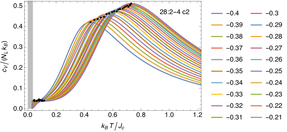
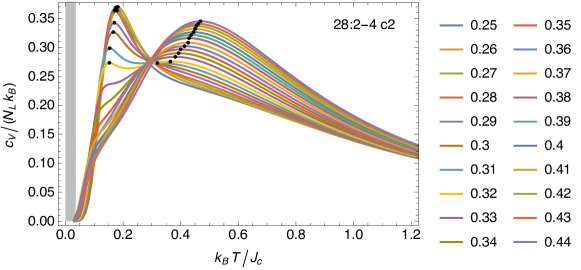
To demonstrate characteristic features, Figs. 7 and 8 show the temperature dependence of the specific heat $c_{V}(T)$ according to Eq. (21) for a selected range of anisotropy parameters $\phi$ in the antiferromagnetic (Fig. 7) and the spiral phase (Fig. 8). The FTLM calculations are trustworthy only down to a temperature range of $T\approx J_{\text{c}}/(Nk_{\text{B}})$. For lower temperatures they are dominated by the artificial finite size gaps. This excluded region is indicated by grey bars in the figures.

For the AF phase with values $-0.4\leq\phi/\pi\leq-0.21$ a single peak indicated by dots that shifts continuously to higher values with increasing $\phi$ is observed. This is qualitatively clear already from the eight-site spectrum (Fig.5) which shows an increasing average excitation gap from the ground state in that range of $\phi$. Furthermore a plateau (or very flat second maximum) at the lowest temperatures close to the finite size gap region is visible.

For the spiral phase the values $0.25\leq\phi/\pi\leq 0.44$, correspond to the region between the isotropic triangular lattice with $J_{2}/J_{1}=1$ and deep inside the disordered phase with quasi-one-dimensional chains ($J_{2}/J_{1}\approx 5$). The tile 28:2-4 was used for the numerical calculations in both cases.

In Fig. 8, the characteristic maxima of $c_{V}(T)$, indicated by the small black dots in the figure, have positions which fall into two different temperature ranges: For the isotropic triangular case with $\phi/\pi=0.25$, the maximum sits at $T_{\triangle}\approx 0.18J_{\text{c}}/k_{\text{B}}$, reducing in magnitude and shifting slightly to lower temperatures $T_{\triangle}\approx 0.15J_{\text{c}}/k_{\text{B}}$ upon increasing $\phi$ from its isotropic value to $\phi/\pi\approx 0.31$ or $J_{2}/J_{1}\approx 1.5$. At this point, a second maximum develops starting at $T_{\parallel}\approx 0.32J_{\text{c}}/k_{\text{B}}$, shifting to higher temperatures as $\phi$ is increased towards the disordered region. Furthermore, the maximum $T_{\triangle}$ characteristic for the triangular lattice rapidly disappears with increasing $\phi$. Only the $C_{V}(T)$ curves for $\phi/\pi=0.31$ and $\phi/\pi=0.32$ show both maxima simultaneously. At high temperatures $T\gg J_{\text{c}}/k_{\text{B}}$, all the curves show the $(1/T)^{2}$ temperature dependence expected from Eq. (13).

V.2 Exchange anisotropy dependence of peak position and value

Figure 9: Maximum positions (top) and values (bottom) of the specific heat $c_{V}(T)$ as a function of the anisotropy parameter $\phi$. Solid lines: exact solution for tile 8:2-2, squares: tile 16:4-0, triangles: tile 20:2-4, diamonds: tile 24:4-0, filled circles: tile 28:2-4. The white rings mark the corresponding exact values for the one-dimensional chain Bonner and Fisher (1964).

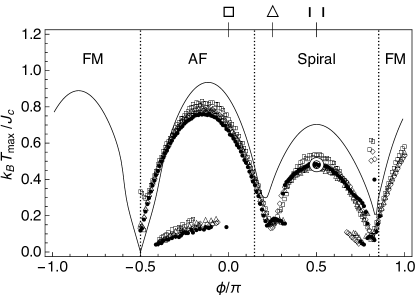
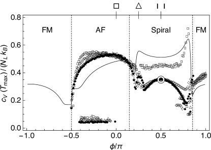
Fig. 9 shows a compilation of the maximum positions and values of $c_{V}(T)$ for the five different tiles we have used as a function of the anisotropy parameter $\phi$. The solid lines denote the exact solution for the tile 8:2-2, see Eq. (9) and Table 1. The black dots denote the maxima for the tile 16:4-0, the open triangles for the tile 20:2-4, the solid diamonds for the tile 24:4-0, the open squares for the tile 28:2-4. Furthermore, the exact results taken from Ref. Bonner and Fisher (1964) for the one-dimensional chain, $c_{V}(T_{\text{max}})/(N_{\text{L}}k_{\text{B}})=0.35$ and $k_{\text{B}}T_{\text{max}}/J_{\text{c}}=0.481$, are marked with the white circles and serve as a gauge to judge how close a cluster of given size approaches the thermodynamic limit.

The eight-site cluster, introduced as an illustration of the model and its overall spectrum, clearly is not very useful quantitatively to discuss the heat capacity in the thermodynamic limit. Only the overall behavior of the maximum temperature is qualitatively similar to our findings for the larger tilings, however the two minima in the spiral phase are shifted towards the classical phase borders. The values $c_{V}(T_{\text{max}})$ for the eight-site cluster are monotonically increasing in the antiferromagnetic phase, followed by a minimum at $\phi/\pi\approx 0.1$ and a maximum at the isotropic point, $\phi/\pi=0.25$. On the ferromagnetic-$J_{1}$ side for $1/2<\phi/\pi\leq 1$, $c_{V}(T_{\text{max}})$ increases again to a second maximum, followed by a minimum at the crossover to the ferromagnet at $J_{2}/|J_{1}|=1/2$. At the one-dimensional point $J_{1}=0$, naturally both $T_{\text{max}}$ and $c_{V}(T_{\text{max}})$ differ strongly from the exact values.

Also the 16-site tiling shows similar features. For the larger clusters of size $N=20$ and more, both maximum temperature positions and maximum values of the specific heat clearly show a double-peak structure as function of $\phi$. The positions $T_{\text{max}}$ decrease with increasing cluster size, apart from the regions around the isotropic point and in the spiral phase near the ferromagnet. At the one-dimensional point, agreement with the infinite-chain result Bonner and Fisher (1964) (white circles) is achieved already with $N=20$ tiling. And therefore results for the $N=28$ tile represent well the thermodynamic limit as far as peak position and height is concerned. Denoting the largest value in each sector of Fig. 9 by $T^{*}_{\text{max}}$ we observe that $T^{*}_{\text{max}}(\text{AF})/T^{*}_{\text{max}}(\text{spiral})=1.58$. This asymmetry in $T_{\text{max}}(\phi)$ is considerably larger than the corresponding one in the square lattice $J_{1}$-$J_{2}$ model where $T^{*}_{\text{max}}(\text{AF})/T^{*}_{\text{max}}(\text{CAF})=1.26$. (The columnar AF (CAF) phase replaces the spiral phase in this model.) Similarly for the asymmetry ratios of peak values in the triangular case we get $c_{V}[T^{*}_{\text{max}}](AF)/c_{V}[T^{*}_{\text{max}}](\text{spiral})=1.51$ much larger than $c_{V}[T^{*}_{\text{max}}](AF)/c_{V}[T^{*}_{\text{max}}](\text{CAF})=1.10$ in the square lattice. Inside the AF and spiral sectors the lowest $T_{\text{max}}$ is reached close to the isotropic triangular point with $T^{\triangle}_{\text{max}}\approx 0.18J_{\text{c}}/k_{\text{B}}$ because there exchange frustration is most pronounced (Fig. 3). This leads to a high density of low energy excitations (c.f. Fig. 5) and therefore a low $T^{\triangle}_{\text{max}}$.

Furthermore, in parts of the antiferromagnetic as well as the spiral phase, a second maximum $c_{V}(T_{\text{max}2})$ at very low temperatures appears. $T_{\text{max}2}$ depends roughly linearly on $\phi$ while $c_{V}\left(T_{\text{max}2}\right)$ remains constant and small, see also Fig. 7. With the 28-site tiling being the largest possible, we cannot judge whether this second-low temperature maximum in the antiferromagnetic phase merely is a finite-size effect. This is different from the situation in the spiral phase, where the partially observed second maximum is at temperatures $T_{\text{max}2}$ far larger than the finite-size gap, see also Fig. 8.

Similar to the behavior around the isotropic point, at the crossover to the ferromagnetic region a second maximum gradually appears in $c_{V}(T)$ which then evolves to the “ferromagnetic” maximum while the “spiral” maximum disappears. This also happens at comparatively low temperatures with an irregular behavior of the maximum values as function of $\phi$. We attribute this irregularity to the fact that in particular near the borders of the spiral phase the ground state and possible low-lying excited states have incommensurate ordering vectors ${\bf Q}={\bf Q}_{\text{AF}}+\delta{\bf Q}$ and ${\bf Q}_{\text{FM}}+\delta{\bf Q}$ respectively with $|\delta{\bf Q}|\ll 1$. These are not contained in the coarse grid of crystal momenta of our finite tiles.

VI Susceptibility

Figure 10: Maximum positions (top) and values (bottom) of the static susceptibility $\chi(T)$ as a function of the anisotropy parameter $\phi$. Solid lines: exact solution for tile 8:2-2, squares: tile 16:4-0, triangles: tile 20:2-4, diamonds: tile 24:4-0, filled circles: tile 28:2-4. The white rings mark the corresponding exact values for the one-dimensional chain Bonner and Fisher (1964).

Figure 11: Temperature dependence of the static susceptibility $\chi(T)$ of the anisotropic triangular lattice according to Eq. (20) for anisotropy parameters $\phi$ in the spiral phase ranging between $\phi/\pi=0.57$ and $\phi/\pi=0.86$, see legend. We used tile 28:2-4 for the numerical evaluation of Eq. (20), the gray-shaded area at low temperatures illustrates the finite-size gap of order ${\cal O}(J_{\text{c}}/N)$. The characteristic maxima of $\chi(T)$ are indicated by the small black dots.

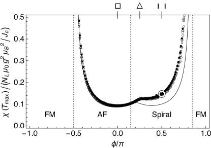
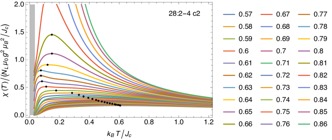
Evaluation of the susceptibility with FTLM is more involved because it requires the calculation of magnetic moment matrix elements. On the other hand this quantity can be more easily compared to experimental results. Most known exchange parameters for spin systems are due to the application of this method.

VI.1 Temperature dependence

Similar to the specific heat, we have calculated the temperature dependence of the static magnetic susceptibility $\chi(T)$ according to Eq. (20) with the tilings shown in Fig. 6. Fig. 11 shows the results in a selected range of the anisotropy parameter, $0.57\leq\phi/\pi\leq 0.86$, calculated with tiling 28:2-4. This parameter range corresponds to the interpolation between ferromagnetically coupled ($J_{1}<0$) quasi-one-dimensional antiferromagnetic chains with $J_{2}/J_{1}\approx-4.5$ and the crossover to the ferromagnet at the classical boundary $J_{2}/J_{1}=-1/2$. For the former, a very broad maximum is characteristic which gradually evolves into the $T=0$ divergence of $\chi(T)$ in the ferromagnetic phase, which is the expected behavior.

VI.2 Exchange anisotropy dependence

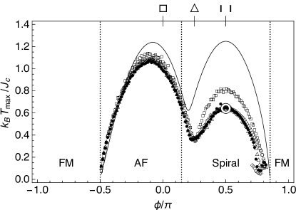
In the same way as for the specific heat, we follow the positions and values of the characteristic maxima of $\chi(T)$ as a function of the anisotropy parameter, using the tiles displayed in Fig. 6 again. This is shown in Fig. 10. The solid lines denote the eight-site results according to Eq. (8). For the same reasons as discussed for the heat capacity, strong deviations from the larger tilings occur in particular in the spiral phase. In contrast to $c_{V}(T)$, the maximum positions and values of $\chi(T)$ are already converged for tilings of size $N=20$ and larger, apart from the crossover to the ferromagnetic phase, where a tile-dependence of the maximum temperatures clearly can be observed.

Similar as for the specific heat the $T_{\text{max}}(\phi)$ dependence has a pronounced asymmetry in AF and spiral sectors. Denoting again the largest value in each sector by $T^{*}_{\text{max}}$ we obtain for the triangular lattice $T^{*}_{\text{max}}(\text{AF})/T^{*}_{\text{max}}(\text{spiral})=1.58$ which is much larger than the asymmetry value $T^{*}_{\text{max}}(\text{AF})/T^{*}_{\text{max}}(\text{CAF})=1.11$ for the square lattice case. Similar to specific heat behavior the $T_{\text{max}}(\phi)$ minimum inside AF and spiral sectors is reached around the most frustrated isotropic triangular position $T^{\triangle}_{\text{max}}\approx 0.35J_{\text{c}}/k_{\text{B}}$.

At the one-dimensional point, as for the heat capacity, the results from Ref. Bonner and Fisher (1964), $k_{\text{B}}T_{\text{max}}/J_{\text{c}}=0.641$ and $\chi(T_{\text{max}})/(N_{\text{L}}\mu_{0}(g\mu_{\text{B}})^{2}/J_{\text{c}})=0.147$ are accurately reproduced with our method. In general we think that in particular our results on the magnetic susceptibility can be used to accurately determine both exchange constants $J_{1}$ and $J_{2}$ individually, which we show in the following section.

VII Application to Cs${}_{\text{2}}$CuCl${}_{\text{4}}$ and Cs${}_{\text{2}}$CuBr${}_{\text{4}}$

Figure 12: Temperature dependence of the magnetic susceptibility $\chi(T)$ of Cs${}_{\text{2}}$CuCl${}_{\text{4}}$ (dots and solid line) and Cs${}_{\text{2}}$CuBr${}_{\text{4}}$ (open circles and dashed line). The top plot displays the experimental data (symbols, taken from Ref. Cong et al. (2011)) together with the fits of our FTLM data (lines, fitted values see Table 2). The bottom plot displays exactly the same data, this time in dimensionless units using $J_{\text{c}}$, $\phi$, and $g$ for the two compounds from Table 2.

Table 2: Comparison of exchange parameters for Cs${}_{\text{2}}$CuCl${}_{\text{4}}$ and Cs${}_{\text{2}}$CuBr${}_{\text{4}}$ as determined from thermodynamic FTLM-fit and direct spectroscopic INS (Cs${}_{\text{2}}$CuCl${}_{\text{4}}$ only) and ESR methods at $H>H_{\text{sat}}$. Exchange constant $J_{2}$ corresponds to the crystallographic $b$ direction and $J_{1}$ to the zigzag bonds in the $bc$ plane.

compound	method	$J_{1}/\text{meV}$	$J_{2}/\text{meV}$	$J_{\text{c}}/\text{meV}$	$J_{2}/J_{1}$	$\phi/\pi$	$g$	Ref.
Cs${}_{\text{2}}$CuCl${}_{\text{4}}$	FTLM	$0.11$	$0.38$	$0.40$	$3.45$	$0.41$	$2.06$	this work
	INS	$0.128$	$0.374$	$0.40$	$2.92$	$0.40$	$2.19$	Coldea et al. (2002)
	ESR	$0.12$	$0.41$	$0.43$	$3.42$	$0.41$	$2.08$	Zvyagin et al. (2014)
Cs${}_{\text{2}}$CuBr${}_{\text{4}}$	FTLM	$0.5$	$1.26$	$1.35$	$2.52$	$0.38$	$2.04$	this work
	ESR	$0.53$	$1.28$	$1.38$	$2.44$	$0.38$	$2.09$	Zvyagin et al. (2014)

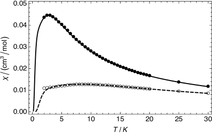
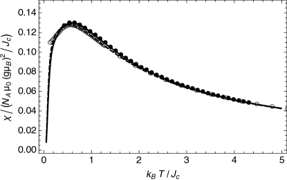
As a demonstration of the usefulness of the method, we apply our findings to the compounds Cs${}_{\text{2}}$CuCl${}_{\text{4}}$ and Cs${}_{\text{2}}$CuBr${}_{\text{4}}$. Fig. 12 shows the temperature dependence of the magnetic susceptibility. The dots and the open circles denote the experimental data taken from Ref. Cong et al. (2011), the solid and dashed lines denote the corresponding fits with our FTLM data. In order to avoid misunderstandings, we have plotted the data and the curves in two different ways: The top plot in Fig. 12 displays $\chi(T)$ in electromagnetic (CGS) units from where we have determined the values for our model parameters reproduced in Table 2. Using these fitted values for $J_{\text{c}}$, $\phi$, and $g$, we have plotted the same data again in dimensionless units in the bottom plot of Fig. 12. The main effect of replacing Cl with Br is an increase of the overall energy scale $J_{\text{c}}$ by a factor $3.4$, whereas the anisotropy angle $\phi$ changes only by about $5\,\%$. Thus only this large change in $J_{\text{c}}$ is responsible for the decrease of the maximum in $\chi(T)$, the broadening of the maximum, and the shift of the maximum towards higher temperatures. The anisotropy ratio and therefore the position of Cs${}_{\text{2}}$CuBr${}_{\text{4}}$ in the phase diagram remains essentially the same as for Cs${}_{\text{2}}$CuCl${}_{\text{4}}$, it is only slightly moved away from the quasi-one-dimensional regime. Historically the first measurement of $\chi(T)$ of Cs${}_{\text{2}}$CuCl${}_{\text{4}}$ yielded slightly different values Carlin et al. (1985), however the data analysis was performed over a limited temperature range assuming weakly coupled one-dimensional chains.

As pointed out in Sec. V.1, the steep decrease of $\chi(T)$ for $T\to 0$ in both cases is an artifact of the finiteness of the tiling used for the FTLM calculations. Assuming a finite-size gap $\Delta\approx J_{\text{c}}/N$, the corresponding temperatures where we expect finite-size effects to dominate are $T_{\Delta}\approx 0.2\,\text{K}$ for Cs${}_{\text{2}}$CuCl${}_{\text{4}}$ and $T_{\Delta}\approx 0.6\,\text{K}$ for Cs${}_{\text{2}}$CuBr${}_{\text{4}}$. Experimentally, the lowest temperature was $T_{\text{min}}\approx 2\,\text{K}$, well above the finite-size gaps.

Our result from the FTLM fit to thermodynamic data are compared in Table 2 to results from direct spectroscopic methods: Inelastic neutron scattering (INS) Coldea et al. (2002) (Cs${}_{\text{2}}$CuCl${}_{\text{4}}$ only) and electron spin resonance (ESR) Zvyagin et al. (2014), both in fields above the saturation field Schmidt and Thalmeier (2014)

$$\mu_{0}H_{\text{sat}}=\frac{2S}{g\mu_{\text{B}}}\frac{(J_{1}+2J_{2})^{2}}{2J_{2}},$$ (22)

which is $\mu_{0}H_{\text{sat}}\approx 8.4\,\text{T}$ for Cs${}_{\text{2}}$CuCl${}_{\text{4}}$ and $\mu_{0}H_{\text{sat}}\approx 30\,\text{T}$ for Cs${}_{\text{2}}$CuBr${}_{\text{4}}$. Taking the spectroscopic data at high fields has the advantage that the ground state is fully polarized, corresponding to a single “all spins up” spinor product state $|\text{FM}\rangle$. The excitations on top of this are the $N$ orthonormal single-particle excitations $|\psi_{i}\rangle=(1/\sqrt{2S})S_{i}^{-}|\text{FM}\rangle$, $i=1\ldots N$ with $N={\cal O}(N_{\text{L}})$. Because $\left[{\cal H},\Omega_{z}\right]=0$, the Hamiltonian can not generate more than these one-spin-flip states, and its spectrum can be determined exactly by Fourier transform.

The agreement between the different methods is almost perfect, for exchange parameters as well as g-factors. As already mentioned in Ref. Schmidt and Thalmeier (2014) if Cs${}_{\text{2}}$CuCl${}_{\text{4}}$ is interpreted as a purely 2D system this set of exchange parameters puts the compound very close to the quasi-1D spin liquid regime centered at $\phi=0.5\pi$. In reality, however, the magnetic order is stabilized below $T_{\text{N}}=0.62$ K by a finite inter-plane coupling of the order $J_{\perp}\approx 0.017\,\text{meV}$ along the crystallographic $a$ direction Coldea et al. (2003).

For Cs${}_{\text{2}}$CuBr${}_{\text{4}}$, we see deviations of the experimental data from our result at the lowest temperatures. These are not due to impurities Cong et al. (2011, 2014), but can be regarded as an indication for a tendency towards magnetic order in this compound. The overall energy scale $J_{\text{c}}$ is more than three times larger than for Cs${}_{\text{2}}$CuCl${}_{\text{4}}$, however the estimate for the anisotropy angle $\phi$ is essentially the same. We therefore expect that Cs${}_{\text{2}}$CuBr${}_{\text{4}}$ orders magnetically as well, possibly at a higher temperature than its Cl counterpart.

The agreement of our thermodynamic analysis with direct spectroscopic results gives us confidence that the FTL method may be applied to the analysis of the whole Cs${}_{\text{2}}$CuCl${}_{\text{4}-x}$Br${}_{\text{x}}$ substitutional series Cong et al. (2011, 2014).

VIII Conclusion and Outlook

In this work we have shown that finite temperature Lanczos method for finite clusters is a versatile tool to investigate the little known finite temperature properties of frustrated triangular quantum magnets, in contrast to QMC approach which is not suitable in this case. The FTL method complements the analytical spin wave approach which is useful only for the very low temperature regime and is a more straightforward alternative to the high temperate series expansion method.

For this quantum spin model one can use a single control parameter and tune the system through the phase diagram where several special cases with very different frustration degree like frustrated Néel, unfrustrated HAF, frustrated spiral and isotropic triangular $120^{\circ}$ phase as well as unfrustrated spin chains and frustrated FM may be realized.

For the largest investigated cluster with $N=28$ sites we obtain a trustworthy representation of the thermodynamic limit behavior since the exact known result for the spin chain case is produced very well and shows little difference to the $N=24$ cluster. As a main result we gave the systematic variation of peak position and peak height of specific heat and susceptibility as function of $J_{2}/J_{1}$. Both values are strongly suppressed for the most frustrated isotropic triangular magnet (Figs. 9 and 10). Furthermore a surprisingly large asymmetry in particular for the maximum position exists between the AF and spiral phase region. It is considerably larger than between the AF and CAF regions in the square lattice $J_{1}$-$J_{2}$ model. In addition we found that the simple single peak shape of $c_{V}(T)$ and $\chi(T)$ may be distorted due to smaller side maxima or shoulders at lower temperature for some ranges of the control parameter.

The most reliable method to extract the exchange parameters is the fitting of $\chi(T)$ over the whole temperature range (above the finite size gap) using FTLM results. We have demonstrated this for two of the most typical 2D triangular magnets, Cs${}_{\text{2}}$CuCl${}_{\text{4}}$ and Cs${}_{\text{2}}$CuBr${}_{\text{4}}$. We have obtained excellent agreement with results from the INS investigation and with ESR results in the fully polarized state. Our method has the additional advantage that it can easily be extended to the whole substitutional series Cs${}_{\text{2}}$CuCl${}_{\text{4}-x}$Br${}_{\text{x}}$ ($0\leq x\leq 4$) Cong et al. (2011) to extract the systematic variation of frustration anisotropy control parameter $\phi$ and energy scale $J_{\text{c}}$ as a function of Br concentration sch . We note that our method can also be applied to magnetocaloric measurements of the organic charge-transfer salts where localized $S=1/2$ magnetic moments are residing on a possibly distorted triangular lattice as well. This includes the Et_xMe_4-xZ$[$Pd$($dmit$)_{2}]_{2}$ ($x=0,1,2$) family of compounds Itou et al. (2008); Tamura et al. (2006) as well as $\kappa$-$($ET$)_{2}$B$($CN$)_{4}$ and $\kappa$-$($ET$)_{2}$Cu${}_{2}($CN$)_{3}$ Yoshida et al. (2015) and $\kappa$-$($BEDT-TTF$)_{2}$Cu$[$N$($CN$)_{2}]$Cl Hamad et al. (2005).