Total, inelastic and (quasi-)elastic cross sections of high energy $\mathrm{p}A$ and $\gamma^{\star}A$ reactions with the dipole formalism

Abstract:

In order to understand the initial partonic state in proton–nucleus and electron–nucleus collisions, we investigate the total, inelastic, and (quasi-)elastic cross sections in $\mathrm{p}A$ and $\gamma^{\star}A$ collisions, as these observables are insensitive to possible collective effects in the final state interactions. We used as a tool the DIPSY dipole model, which is based on BFKL dynamics including non-leading effects, saturation, and colour interference, which we have extended to describe collisions of protons and virtual photons with nuclei. We present results for collisions with O, Cu, and Pb nuclei, and reproduce preliminary data on the pPb inelastic cross section at LHC by CMS and LHCb. The large $NN$ cross section results in $\mathrm{p}A$ scattering that scales approximately with the area. The results are compared with conventional Glauber model calculations, and we note that the more subtle dynamical effects are more easily studied in the ratios between the total, inelastic and (quasi-)elastic cross sections. The smaller photon interaction makes the $\gamma^{\star}A$ collisions more closely proportional to $A$, and we see here that future electron–ion colliders would be valuable complements to the $\mathrm{p}A$ collisions in studies of dynamical effects from correlations, coherence and fluctuations in the initial state in high energy nuclear collisions.

1 Introduction

An important question in the understanding of the strong force is the behaviour of a hot and dense plasma, and properties of the QCD phase diagram, with a possible critical point. We note that it is here very difficult to get definitive answers from ab initio lattice simulations [1, 2]. Results from RHIC, summarised in the “White Papers” by the four collaborations [3, 4, 5, 6], have been interpreted as indicating the dynamics of a nearly perfect fluid. These results were subsequently extended to higher energies and investigated in a broader kinematic range with improved precision by the LHC experiments that have heavy ion programmes. These experiments include ALICE, ATLAS and CMS, and their status during 2014 were summarised for example by references [7, 8, 9]. The $\mathrm{pPb}$ program at the LHC turned out to be very surprising, culminating in observation of signals of collectivity not only in $\mathrm{PbPb}$, but also in $\mathrm{pPb}$ reactions. Recent results from the Beam Energy Scan program at RHIC [10] are adding important elements to the picture in the energy range where many observables change together. These observations have also been interpreted as a signal for a critical point in the theory of strong interactions, QCD, in the vicinity of $(T_{E},\mu_{B,E})=(165,95)$ MeV [11].

It has often been suggested that studies of $\mathrm{p}A$ or $\mathrm{e}A$ scattering can play an important rôle in studies of the transition between the “simpler” $\mathrm{pp}$ or $\mathrm{ep}$ collisions and the more complicated $AA$ collisions. A recent review [12] on $\mathrm{dAu}$ and $\mathrm{pPb}$ collisions at RHIC and LHC, respectively, indicates that many of the signatures of nearly perfect fluid dynamics considered for $\mathrm{AuAu}$ or $\mathrm{PbPb}$ collisions appear also in $\mathrm{d}A$ and $\mathrm{p}A$ collisions at RHIC and LHC energies, thus suggesting that similar perfectly flowing quark matter may be created also in these collisions, although its volume and its lifetime must be smaller than in the corresponding heavy ion collisions. The similarity between $\mathrm{pPb}$ and $\mathrm{PbPb}$ collisions is also emphasised in the CMS overview in ref. [9].

We also note that even high energy $\mathrm{pp}$ collisions exhibit many features interpreted as signals for collective behaviour, such as systematics of single-particle spectra and Bose–Einstein correlation radii [13], the increased production of strange particles and baryons (not least of strange baryons) [14, 15, 16], and signatures expected from hydrodynamic flow like the p$/\pi$ ratio [17] and a near side ”ridge” [18].

Model predictions for final states in $AA$ or $\mathrm{p}A$ collisions depend strongly on the initial conditions obtained from parton–parton sub-collisions. In many analyses the initial conditions are estimated using the Glauber model [19, 20]. Based on multiple diffractive sub-collisions, it automatically satisfies unitarity. It was early pointed out by Gribov [21], that diffractive excitation of the intermediate nucleons gives a significant contribution (on the 10-15% level) to Glauber’s original model. Within the Good–Walker formalism [22] diffractive excitation can be interpreted as a result of fluctuations in the nucleon’s partonic substructure [23]. It was also pointed out by Białas, Bleszyński and Czyż [24] that fluctuations and correlations in the positions of the individual nucleons within a nucleus has an important effect. Such fluctuations also lead to so called quasi-elastic collisions, where the nucleus is diffractively excited. These effects of fluctuations are most easily taken into account in a Monte Carlo (MC) simulation, where it is also easy to account for a realistic nucleon distribution within the nucleus, including correlations from a hard core in the $NN$ interaction (see e.g. refs. [25, 26, 27]).

However, based on independent nucleon–nucleon collisions the Glauber model does not naturally include possible interference effects between partons in different nucleons, and it is also difficult to include uncorrelated fluctuations between the nucleons in a target nucleus. We also note that although Monte Carlos including diffractive excitation are available, see e.g. ref. [28] and further references therein, lacking good experimental data for inelastic diffraction, these corrections are frequently neglected, and the calculations and implementations of the Glauber model are typically based on either the total $NN$ cross section or the inelastic cross section.

The high parton densities at high energy imply, however, that saturation and interference effects ought to be important. To draw firm conclusions about a collective behaviour in the final state interaction, it is therefore crucial to be able to separate features of the initial state from the dynamics of final state interactions. The aim of this paper is to investigate the initial state of a colliding nucleus in greater detail, and to isolate it from effects of final state interactions. To this end we focus on total, elastic, and quasi-elastic cross sections in $\mathrm{p}A$ and $\mathrm{e}A$ collisions, which are insensitive to effects of final state interactions.

Going beyond the standard Monte Carlo implementations of the Glauber model, we are in particular interested in the following features:

• Effects of the partonic substructure in individual nucleons within a nucleus.

• Interference between partons located in different nucleons, but having the same colour.

• Diffractive excitation including high mass diffraction and quasi-elastic scattering.

Saturation and correlation effects are most easily treated in transverse coordinate space. For our analysis we will use the so-called DIPSY model [29, 30, 31, 32], which is based on BFKL evolution but includes essential non-leading-log effects, confinement, and saturation within the evolution. DIPSY was originally developed for $\gamma^{\star}\mathrm{p}$ and $\mathrm{pp}$ collisions, but can be directly extended to model collisions with nuclei [33]. Besides making it easier to include correlations, fluctuations, and diffraction, the formulation in transverse coordinate space also makes the extension to model realistic nuclei fairly straight-forward. However, as the gluons from different nucleons can interfere, the individual nucleons are not quite independent, and we therefore expect non-trivial effects of shadowing.

The outline of the paper is as follows. First, we will in section 2 briefly go through the theoretical foundation of the dipole formalism and its implementation in the DIPSY Monte Carlo. Section 3 deals with the modifications introduced in DIPSY to simulate collisions including heavy ions, and the way we distribute the nucleons inside a nucleus. In section 4 we first demonstrate that DIPSY reproduces total $\mathrm{pp}$ and preliminary $\mathrm{p}A$ cross sections from RHIC to LHC energies ($\sqrt{s_{(NN)}}=200$ GeV to 8 TeV), before we describe our results and predictions for the total, inelastic, and (quasi-)elastic $\mathrm{p}A$ and $\gamma^{\star}A$ cross sections. In section 5 we discuss the interpretation of the results, and end the paper with a conclusion and outlook in section 6.

2 The Lund Dipole Cascade Model DIPSY

Most event generator models of hadronic interactions at high energies are based on multi-parton interactions, some examples are PYTHIA [34], HERWIG [35], DTUJET [36] and EPOS-LHC [37]. The strongly rising parton distributions for small $x$, consistent with BFKL evolution (albeit with important non-leading effects), make the parton–parton cross sections very large. At higher energies, non-linear effects therefore become increasingly important, and these effects are further enhanced in collisions with nuclei. The non-linear effects depend on the extension of the cascades in transverse space (see the pioneering work by Gribov, Levin, and Ryskin (GLR) [38]). While models for hadronic collisions generally are formulated in momentum space, analyses of saturation and non-linear effects are therefore more easily treated in transverse coordinate space and rapidity.

Formalisms for interactions with high density targets often assume a homogenous target with no boundary effects (which facilitates the calculation of analytic results), and many applications are based on the Color Glass Condensate (CGC) [39] or the BK equation [40, 41]. Here also effects of correlations and fluctuations are frequently neglected.

The DIPSY model was first developed for hadronic collisions and DIS, but could also be directly applied to collisions with nuclei [42]. Implemented in the form of a Monte Carlo event generator, it can easily take into account effects of correlations, fluctuations, and finite nuclear geometry. When modelling $\mathrm{p}A$ or $AB$ nuclear reactions with DIPSY it is assumed that these interactions are dominated by absorption into inelastic channels. Thus the imaginary part of the $S$-matrix is neglected, and the total, elastic, and quasi-elastic cross sections are directly obtained via the optical theorem. The assumed reality of the $S$-matrix also implies that it is possible to take the Fourier transform of the amplitude in $b$-space. This method was applied to obtain the differential elastic cross section $d\sigma/dt$ of $\mathrm{pp}$ collisions from DIPSY in ref. [42].

2.1 Dipole evolution in transverse coordinate space

The DIPSY model is based on Mueller’s dipole cascade model [43, 44, 45], which is a formulation of leading-log BFKL evolution[46, 47] in transverse coordinate space. Mueller’s model relies on the fact that initial-state radiation from a colour charge (in a quark or a gluon) within a hadron is screened at large transverse distances by an accompanying anti-charge, and that gluon emissions therefore can be described in terms of colour-dipole radiation. Thus the partonic state is described in terms of dipoles in impact-parameter space, evolved in rapidity when a dipole is split into two dipoles by gluon emission. The screening implies a suppression of large dipoles in transverse coordinate space, which is equivalent to the suppression of small $k_{\perp}$ in the conventional BFKL evolution in momentum space.

For a dipole with charges at the transverse points $\mathbf{x}$ and $\mathbf{y}$, the probability per unit rapidity ($Y$) to emit a gluon at $\mathbf{z}$ is given by

$$\frac{d\mathcal{P}_{g}}{dY}=\frac{\bar{\alpha}}{2\pi}d^{2}{\mbox{\boldmath$z$}}\frac{({\mbox{\boldmath$x$}}-{\mbox{\boldmath$y$}})^{2}}{({\mbox{\boldmath$x$}}-{\mbox{\boldmath$z$}})^{2}({\mbox{\boldmath$z$}}-{\mbox{\boldmath$y$}})^{2}}\,,\,\,\,\,\,\,\,\mathrm{with}\,\,\,\bar{\alpha}=\frac{N_{c}\alpha_{s}}{\pi}.$$ (1)

The emission produces two new dipoles, $({\mbox{\boldmath$x$}},{\mbox{\boldmath$z$}})$ and $({\mbox{\boldmath$z$}},{\mbox{\boldmath$y$}})$, which can split independently by further gluon emissions. Repeated emissions form a cascade, with dipoles connected in a chain. The chain can be thought of as dipoles connected by gluons, or gluons connected by dipoles [48]. When two cascades collide, a dipole $({\mbox{\boldmath$x$}}_{1},{\mbox{\boldmath$y$}}_{1})$ in a right-moving cascade can interact with a left-moving dipole $({\mbox{\boldmath$x$}}_{2},{\mbox{\boldmath$y$}}_{2})$, with probability (in Born approximation)

$$P_{12}=\frac{\alpha_{s}^{2}}{4}\left[\ln\left(\frac{({\mbox{\boldmath$x$}}_{1}-{\mbox{\boldmath$y$}}_{2})^{2}({\mbox{\boldmath$y$}}_{1}-{\mbox{\boldmath$x$}}_{2})^{2}}{({\mbox{\boldmath$x$}}_{1}-{\mbox{\boldmath$x$}}_{2})^{2}({\mbox{\boldmath$y$}}_{1}-{\mbox{\boldmath$y$}}_{2})^{2}}\right)\right]^{2}.$$ (2)

We note that in this leading log approximation, the probability for dipole emission in eq. (1) diverges for small dipole sizes $({\mbox{\boldmath$x$}}-{\mbox{\boldmath$z$}})$ or $({\mbox{\boldmath$z$}}-{\mbox{\boldmath$y$}})$, but as the interaction probability in eq. (2) then goes to zero, the total cross section is finite. (This is naturally related to colour transparency.) Although the final result is finite, the divergence causes numerical problems in a leading log Monte Carlo simulation [49]. This problem is removed by the non-leading effects included in DIPSY, which suppress very small dipoles.

Via the optical theorem the expression in eq. (2) also equals twice the elastic dipole–dipole scattering amplitude. (As mentioned above we assume that the interaction is driven by the inelastic absorption.) Denoting the right-moving dipoles $i$ and the left-moving $j$, the total elastic scattering amplitude is in the Born approximation given by $F=\sum_{ij}P_{ij}/2$. Multiple scatterings are taken into account in the eikonal approximation via the unitarized elastic amplitude (defined by the relation $S\equiv 1-T$, which makes $T$ real)

$$T=1-\exp{(-F)}=1-\exp{(-\sum P_{ij}/2)}.$$ (3)

To get the full elastic amplitude we also have take the average over all possible cascades. In impact parameter space, the differential total and elastic cross sections are then, via the optical theorem, given by

$$d\sigma_{\mathrm{tot}}/d^{2}b = 2\langle T\rangle,$$

$$d\sigma_{\mathrm{el}}/d^{2}b = \langle T\rangle^{2}.$$ (4)

The cross section for diffractive excitation can be obtained in the Good–Walker [22] formalism, which is described in appendix A. (Diffractive excitation is usually described in either the Good–Walker or the triple-reggeon formalism, but as demonstrated in ref. [50], for high mass diffraction these are just different sides of the same BFKL evolution dynamics.) Diffractive excitation is here determined by the fluctuations in the scattering process. A proton is a linear combination of all possible parton cascades, and as discussed in refs. [31, 51], we assume that these cascades represent the diffractive eigenstates, which thus can come on shell in the interaction. The cross section for diffractive excitation is thus described by the fluctuations among the possible parton cascades in the projectile and the target.

As described in the Appendix, the total diffractive cross section, including elastic scattering, is obtained by summing over all possible diffractive states, and given by $\langle T^{2}\rangle$. This is the sum of elastic scattering, single diffraction of the projectile or the target, and double diffraction. Single diffraction of the projectile with an elastic target is similarly obtained by summing over all projectile states but keeping the target intact, and then subtract the elastic scattering (which is still given by $\langle T\rangle^{2}$). The result is

$$d\sigma_{\mathrm{SD,p}}/d^{2}b=\langle\langle T\rangle_{t}^{2}\rangle_{p}-\langle T\rangle_{p,t}^{2}.$$ (5)

The averages are here taken over all possible cascades for the projectile ($P$) and the target ($T$), for a fixed impact parameter $b$. (Note again that the amplitude T, given by eq. (3), is a real quantity.)

We note that summing over projectile cascades gives production of all possible cascades limited by the rapidity determined by the Lorentz frame used in the analysis. This gives also the possibility to calculate the differential single diffractive cross section $d\sigma_{\mathrm{SD}}/dM_{X}^{2}$.

Double diffraction is similarly given by total diffraction minus single diffraction and minus elastic scattering, which gives the result

$$d\sigma_{\mathrm{DD}}/d^{2}b=\langle T^{2}\rangle_{P,T}-\langle\langle T\rangle_{T}^{2}\rangle_{P}-\langle\langle T\rangle_{P}^{2}\rangle_{T}+\langle T\rangle_{P,T}^{2}.$$ (6)

2.2 Beyond leading log

In a series of papers [29, 30, 31, 32] a generalisation of Mueller’s model, implemented in the Monte Carlo event generator DIPSY, has been described in detail. Here we will only discuss the main points. The basic idea behind the model is to include important non-leading effects in the BFKL evolution, saturation effects within the evolution, and confinement.

The full next-to-leading logarithmic corrections to BFKL have been calculated and have been found to be very large [52, 53]. A physical interpretation of these corrections has been presented by Salam [54], and a dominant part is related to energy-momentum conservation. In the DIPSY model this is achieved by equating the emission of a gluon at small transverse distances with high transverse momenta for the emitted and recoiling gluons. Thus the conservation of energy and momentum implies a dynamic cutoff for very small dipoles with correspondingly high transverse momenta. This constraint has also important computational advantages, removing the divergence in the dipole splitting probability in eq. (1). Other important non-leading effects are the running coupling, $\alpha_{s}(p_{\perp}^{2})$, and the “consistency constraint” or “the energy scale terms”, which implies that the emissions are ordered in both the positive and negative light-cone components [55, 56, 57].

2.3 Nonlinear effects

Besides these perturbative corrections, confinement effects are included via a small gluon mass, and non-linear saturation effects through the so-called swing mechanism, which is a colour suppressed correction to the cascade evolution. Mueller’s dipole evolution is derived in the large $N_{c}$ limit, where each colour charge is uniquely connected to an anti-charge within a dipole. Saturation effects are here included as a result of multiple dipole interactions, in the frame used for the analysis. Such multiple interactions give dipole chains forming loops (see ref. [30]), and are related to multiple pomeron exchange. When multiple interactions can be neglected, Mueller’s model gives a result, which is independent of the Lorentz frame used for the calculation  [58]. Loops formed within the evolution are, however, not included. This means that when multiple interactions cannot be neglected, the result is no longer frame independent. (Loops within the evolution are also neglected e.g. in the non-linear BK equation [40, 41].)

The dipole interaction in eq. (2) is proportional to $\alpha_{s}$, and thus colour suppressed compared to the dipole splitting in eq. (1). Loop formation is therefore related to the possibility that two dipoles have identical colours. For two dipoles with the same colour, we have actually a colour quadrupole, where a colour charge is effectively screened by the nearest anti-colour charge. Thus approximating the field by a sum of two dipoles, one should preferentially combine a colour charge with a nearby anti-charge. This interference effect is taken into account in DIPSY in an approximate way, by allowing two dipoles with the same colour to recouple forming new dipoles, in a way favouring small dipoles. This mechanism, called a swing, is illustrated in figure 1; see further ref. [30].

Figure 1: Two dipoles with the same colour, forming a colour quadrupole, may be better approximated by two dipoles formed when the colour charges are recoupled, as illustrated here.

Although this recipe is an approximation, the dependence on the Lorentz frame used for calculating the cross section is significantly reduced, as demonstrated and detailed in  section 5.2.

In the simulation the swing is handled by assigning all dipoles a colour index running from 1 to $N_{c}^{2}$, not allowing two dipoles connected to the same gluon to have the same index. A pair of two dipoles, $({\mbox{\boldmath$x$}}_{1},{\mbox{\boldmath$y$}}_{1})$ and $({\mbox{\boldmath$x$}}_{2},{\mbox{\boldmath$y$}}_{2})$, having the same colour, may be better approximated by the combination $({\mbox{\boldmath$x$}}_{1},{\mbox{\boldmath$y$}}_{2})$ and $({\mbox{\boldmath$x$}}_{2},{\mbox{\boldmath$y$}}_{1})$, if these dipoles are smaller. In the evolution the pair is allowed to “swing” back and forth between the two possible configurations shown in figure 1. The swing mechanism is adjusted to give the relative probabilities $({\mbox{\boldmath$x$}}_{1}-{\mbox{\boldmath$y$}}_{2})^{2}({\mbox{\boldmath$x$}}_{2}-{\mbox{\boldmath$y$}}_{1})^{2}:({\mbox{\boldmath$x$}}_{1}-{\mbox{\boldmath$y$}}_{1})^{2}({\mbox{\boldmath$x$}}_{2}-{\mbox{\boldmath$y$}}_{2})^{2}$, thus favouring the configuration with smallest dipoles. In the evolution in rapidity, the swing is competing with the gluon emission in eq. (1), where a Sudakov-veto algorithm [59] can be used to choose which of the two happens first.

The non-linear GLR [38] and BK [40, 41] equations are formulated in a way where the number of dipoles can be reduced, via a $(2\rightarrow 1)$ vertex. What is calculated in these formalisms is actually the interaction probability. With the swing mechanism the number of dipoles is unchanged. However, as the dipole swing leads to smaller average dipole sizes, the interaction probability in eq. (2) is also reduced in accordance with colour transparency. Thus the swing represents a similar kind of physics as these evolution equations. An advantage with the DIPSY formalism is that it is possible to also take into account correlations [60], fluctuations, and effects of the nuclear size and shape.

2.4 Final states

The BFKL equation and Mueller’s model describe the inclusive cross section, but as seen from the CCFM formalism [55, 61] it is possible to include softer gluon emissions to form exclusive final states. As described in ref. [56] in the Linked Dipole Chain model (LDC), these softer gluons can be added as final state radiation from an initial BFKL ladder. When the two evolved systems collide, some of the dipoles in the right-moving system interact with some in the left-moving one, and the cross sections are calculated via eqs. (1) - (4). The interaction enables the gluons in the interacting dipoles to come on-shell, together with all parent dipoles, while non-interacting dipoles must be regarded as virtual and thus be reabsorbed. In a situation, where saturation is important, it is also necessary to include possible swings in the final state [30, 62]. In the DIPSY MC the gluons are traced in both momentum and coordinate space, and therefore the model also allows us to generate the final-state momentum distribution of gluons and, after hadronization, final hadronic states [32, 62]. In the present paper we restrict our study to inclusive total and inelastic cross sections, while final states will be studied in future work on $\mathrm{p}A$ and $\mathrm{e}A$ collisions.

The stochastic nature of BFKL evolution also implies, that the exclusive final states obtained in an event generator like DIPSY, includes fluctuations and correlations which are essential for many observables. As an example, we note that the fluctuations in the scattering amplitude determines the cross section for diffractive excitation in eq. (4).

2.5 The Monte Carlo event generator DIPSY

The Lund Dipole Cascade Model has been implemented in the Monte Carlo event generator called DIPSY, with applications mainly to $\mathrm{pp}$ collisions and DIS. In a high energy collision, two hadrons are evolved from their respective rest frames to a Lorentz frame in which they collide. In its own rest system a proton is currently modelled by a simple triangle of gluons connected by dipoles, and the gluonic Fock state is built by successive dipole emissions of virtual gluons. The small-$x$ partons are dominated by gluons, and the result for small $x$ is rather insensitive to the choice of initial parton configuration, apart from its overall size. We also note that the proton structure functions are well reproduced by the DIPSY model [63]. (Quarks are important for the final state, and here valence quarks are later introduced by hand).

The parameters of the MC model have been tuned to the energy dependence of the total and elastic $\mathrm{pp}$ scattering cross sections. The best values of the tune parameters that govern the calculations will be shown and discussed in section 4.1. Since the system at very large energies is dominated by gluons, the model may use the same parameters later on for all kinds of reactions and observables.

Here, we show the list of the parameters whose values substantially influence the final results. They are described in more detail for example in ref. [42].

• $R_{max}$: Non-perturbative regularisation scale, this corresponds to the maximum dipole size in a given simulation, above which emissions and interactions are exponentially suppressed [31]. Its typical value is $\approx 3$ GeV^-1.

• $R_{p}$: The average size of the proton at rest. Its typical value is $\approx 3$ GeV^-1.

• $w_{p}$: The width of the Gaussian fluctuations in proton size around $R_{p}$. As in ref. [42] this value was set to 0.1 GeV^-1.

• $\Lambda_{QCD}$: This is the scale parameter of $\alpha_{s}$, the running coupling constant of QCD, and its default value in the present calculations was 0.23 GeV.

• $\lambda_{r}$: This parameter controls the swing effect, its default value in the presented calculations was 1. Dipoles with the same colour are allowed to swing back and forth, which results in an equilibrium, where the smaller dipoles have a larger weight. $\lambda_{r}=1$ has previously [32] been shown to be large enough to reach the equilibrium.

3 Treatment of nuclei in DIPSY

The DIPSY model, initially developed for $\mathrm{ep}$ and $\mathrm{pp}$ collisions, can be directly generalised to simulate collisions with nuclei. We just have to generate random positions for all the nucleons within a target nucleus, and let them collide with a projectile proton, a virtual photon, or a similarly generated projectile nucleus. In the present paper we will focus on high energy $\mathrm{p}A$ and $\gamma^{\star}A$ scattering, and of particular interest will here be effects of colour interference between different nucleons in a nucleus, and effects of fluctuations, both in the distribution of nucleons in a nucleus, and in the parton evolution inside individual nucleons.

High energy nuclear collisions are usually analysed within the Glauber formalism [64, 19]. Here it is assumed that the projectile nucleon(s) travel along straight lines and undergo multiple diffractive sub-collisions. Inspite of its pure geometric approach, it has been quite successful in describing many characteristics of reactions with nuclei, and has been widely used in experiments at RHIC and LHC, e.g. to estimate the number of binary nucleon–nucleon collisions and the number of participant nucleons as a function of centrality. In order to illustrate some features of our results, we will below also make comparisons with Glauber simulations.

Concerning fluctuations we note that there are two different origins for fluctuations i collisions with nuclei. The first is due to fluctuations in the position of the nucleons in a nucleus, while the second is related to diffractive excitation of the wounded nucleons. As described in section 2.1, diffractive excitation of a proton is determined by fluctuations in the internal proton substructure, as given by the Good–Walker formalism. The two effects, and their relation to the Glauber formalism, will be described in sections 3.1 and 3.2. The Good–Walker formalism can also be directly applied to calculate quasi-elastic scattering, where the nucleus is breaking up. This is also discussed in section 3.2.

A very interesting question is also to what extent colour charges in one nucleon can screen charges in other nucleons. In DIPSY this interference effect is described by the swing mechanism, discussed in section 2.3, and in a nucleus we also allow dipoles in different nucleons to swing. The result is a kind of colour reconnection, and in the analysis of our results we will compare the outcome with and without this inter-nucleon swing. Such possible interference effects between the different nucleons are not taken into account in the Glauber approach.

3.1 Distribution of nucleons in a nucleus

It was early pointed out by Białas, Bleszyński and Czyż [24] that fluctuations and correlations in the positions of the individual nucleons within a nucleus has an important effect. This effect, which is most easily taken into account using MC simulation techniques (not easily available at the time) has been studied by several authors, see e.g. refs. [27, 65]. The nucleon positions are typically generated so as to reproduce the charge density observed in $\mathrm{e}A$ scattering, and the hard core in the $NN$ interaction has an important effect reducing the fluctuations in the distributions.

The GLISSANDO method

We will in our simulations follow the method in the GLISSANDO MC [25, 26], to generate the nucleon distributions. The nucleon positions are generated according to a Wood–Saxon distribution for the nucleons, with the following form:

$$\rho(r)=\frac{\rho_{0}(1+wr^{2}/R^{2})}{1+\exp((r-R)/a)}.$$ (7)

Here $R$ is the nuclear radius, $a$ is “skin width”, and $\rho_{0}$ is the central density. The parameter $w$ describes a possible non-constant density, but is zero in the fits to nuclei used in this paper.

The nucleon centres are randomly generated in such a way that the charge distribution determined in ref. [66] is recovered, when the result is convoluted with the charge distribution within nucleons. The nucleons are also generated with a hard-core, which thus introduces short range correlations among the nucleons. As shown by Rybczynski and Broniowski [67], the correct two-particle correlation can be obtained if the nucleons are generated with a minimum distance equal to $2r_{core}$.

We note that if the nucleons are generated within a specific volume, the resulting distribution will (for a finite nucleus) be confined within a smaller volume, and its centre will be shifted. According to ref. [26], the correct charge distribution is, for mass numbers $A>16$, obtained using randomly generated nucleon centres described by the Wood–Saxon form in eq. (7) with the following parameters:

$$R_{NC}=(1.1A^{1/3}-0.656A^{-1/3})\,\,{\rm fm},\,\,\,\,a=0.459\,\,{\rm fm},\,\,\,\,w=0,$$ (8)

together with a hard core with radius $r_{core}=0.45$ fm.

Currently the DIPSY MC includes parametrisations for He, O, Cu, Au, and Pb. (Thus we use the same spherical form also for the light nuclei He and O.) For the nuclei studied in this paper this corresponds to the following radii: $R^{\mathrm{Pb}}_{NC}=6.406$ fm, $R^{\mathrm{Au}}_{NC}=6.288$ fm, $R^{\mathrm{Cu}}_{NC}=4.236$ fm, and $R^{\mathrm{O}}_{NC}=2.511$ fm.

3.2 Diffractive excitation of wounded nucleons

In Glauber’s initial formulation the nucleus was described by a smooth distribution determining the absorption probability, but it was early pointed out by Gribov [21], that effects of diffractive excitation of the wounded nucleons are quite significant. Diffractive excitation occurs when the projectile is a linear combination of states with different absorption probabilities. Diffractive excitation is here determined by the fluctuations in the scattering amplitude, as seen in eq. (23). At lower energies this could be well approximated by a single diffractive state, but it is now well known that diffractive excitation in $\mathrm{pp}$ collisions or DIS is not limited to low masses, and has a high cross section $\sim 10-15\%$ of the total [68, 69, 70]. An important point is here that, due to time dilation, in a $\mathrm{p}A$ collision the state of the projectile is frozen between the sub-collisions, while the target nucleons may all be in different states [71].

As mentioned in the introduction, this effect has been studied in several analyses and, as an example, a model by Strikman and coworkers [72, 28] has been applied by the Atlas collaboration [73]. However, lacking good experimental data for inelastic diffraction, these corrections are frequently neglected, with calculations based on either the total $NN$ cross section or the inelastic cross section (including or excluding diffraction).

In the simplest form of the Glauber Model, the target in a $NN$ collision acts as a black absorber. The projectile nucleon travels along a straight line and interacts inelastically if the transverse distance to a nucleon in the target is smaller than a distance $R$, with

$$\pi R^{2}=\sigma_{\mathrm{in,ND}}^{NN}.$$ (9)

Here $\sigma_{\mathrm{in,ND}}^{NN}$ is the inelastic, non-diffractive nucleon–nucleon cross section. This black-disc approximation implies the following cross sections for nucleon–nucleon collisions (see eqs. (4), (23)):

$$\sigma_{\mathrm{tot}} = 2\int d^{2}b\langle T(b)\rangle=2\pi R^{2}$$

$$\sigma_{\mathrm{el}} = \int d^{2}b\langle T(b)\rangle^{2}=\pi R^{2}$$

$$\sigma_{\mathrm{D}} = \int d^{2}b(\langle T(b)^{2}\rangle-\langle T(b)\rangle^{2})=0$$

$$\sigma_{\mathrm{in,ND}} = \int d^{2}b\langle 1-(1-T(b))^{2}\rangle=\pi R^{2}.$$ (10)

These relations demonstrate, that in a black-disc approximation the diffractive part of the cross section vanishes, and that the elastic and inelastic cross sections are equal, both given by half the total.

The most simple model accounting for diffractive excitation is the so called grey disc model. Here it is assumed that within a radius $R$ the projectile is absorbed with probability $a$, with $0<a<1$. The resulting $\mathrm{pp}$ cross sections are here

$$\sigma_{\mathrm{tot}} = 2\int d^{2}b\langle T(b)\rangle=2\pi R^{2}a$$

$$\sigma_{\mathrm{el}} = \int d^{2}b\langle T(b)\rangle^{2}=\pi R^{2}a^{2}$$

$$\sigma_{\mathrm{D}} = \int d^{2}b(\langle T(b)^{2}\rangle-\langle T(b)\rangle^{2})=\pi R^{2}a(1-a)$$

$$\sigma_{\mathrm{in,ND}} = \int d^{2}b\langle 1-(1-T(b))^{2}\rangle=\pi R^{2}a.$$ (11)

The parameters $R$ and $a$ can now be adjusted to reproduce e.g. the total and the elastic $\mathrm{pp}$ cross sections. It is interesting to note that even in this gray disc limit, $\sigma_{\mathrm{el}}+\sigma_{\mathrm{D}}=\sigma_{\mathrm{in,ND}}=\sigma_{\mathrm{tot}}/2.$ We also note that in the LHC energy region $\sigma_{\mathrm{el}}\approx 0.25\,\sigma_{\mathrm{tot}}$, which in this grey disc model gives $\sigma_{\mathrm{D}}\approx\sigma_{\mathrm{el}}$ and $\sigma_{\mathrm{in,ND}}\approx 0.5\,\sigma_{\mathrm{tot}}$. Also other forms for the $\mathrm{pp}$ interaction have been considered in the literature, e.g. a Gaussian interaction profile [74, 75, 64].

In the black disc approximation the fluctuations are totally neglected. As mentioned above, in a $\mathrm{p}A$ collision the state of the projectile is frozen between the sub-collisions, while the target nucleons may all be in different states. Averaging over different colliding target nucleons therefore tends to reduce the fluctuations. Consequently, if the parameters in the grey disc approximation are adjusted to the total and elastic $\mathrm{pp}$ cross sections, the effects of fluctuations are instead overestimated. The averaging over different states for the target nucleons is properly taken into account in DIPSY, and when comparing the DIPSY results with Glauber calculations we therefore expect the DIPSY to lie in between the black and grey disc results .

As the main difference in $\mathrm{p}A$ collisions between the DIPSY model and Glauber-based models is the treatment of fluctuations inside nucleons, it is interesting to study the diffractive dissociation of the nucleus. From the single diffraction cross section in eq. (5) we immediately get that this is given by

$$d\sigma_{\mathrm{SD,A}}/d^{2}b=\langle\langle T\rangle_{p}^{2}\rangle_{A}-\langle T\rangle_{p,A}^{2}\,\,.$$ (12)

Experimentally this means that we must detect an elastically scattered proton in one direction, and a dissociated nucleus in the other. In DIPSY there is in this case a dependence on the frame in which the collision is studied. Typically the proton–nucleon rest frame is used, which means that we only consider the case where the diffractively dissociated nucleus does not produce particles in the proton hemisphere of the detector.

It should be noted that even if the grey- and black-disc Glauber calculations do not model the single diffractive components for $\mathrm{pp}$ collisions, they will give diffractively dissociated nuclei due to the fluctuations in the distribution of nucleons. This can be thought of as elastic scattering of the proton with one of the nucleons, causing the nucleus to break up.

Experimentally it may be difficult to measure low-mass diffraction in the nucleus direction, and below we will also study what we call quasi-elastic scattering, where again the proton is scattered elastically, but the only other requirement is that the proton hemisphere of the detector is empty. This corresponds to adding the single diffractive and elastic cross sections, resulting in

$$d\sigma_{\mathrm{el*}}/d^{2}b=\langle\langle T\rangle_{p}^{2}\rangle_{A}\,\,.$$ (13)

4 Monte Carlo cross section results

In this section we present various Monte Carlo simulation results for high energy proton–proton, proton–ion, photon–proton and photon–ion reaction cross sections performed by DIPSY. In order to show that these numbers are reasonable, they are compared to (preliminary) data, where these data are already available. Most of the (heavy) ion results ($\mathrm{p}A$ and $\gamma^{\star}A$) are in fact predictions, given that the corresponding experimental values are not yet measured and many of these determinations are not even foreseen at present.

As discussed in section 1, our calculations are based on the evolution and interaction of virtual gluons whose number is increasing with the increase of $\sqrt{s}$ and the size of the nuclei involved. As a practical consequence, the simulations for more energetic reactions and higher values of A are limited by the available computational power to achieve reasonable statistics in reasonable time. The scope of this paper, due to this practical consideration, covers ranges of centre-of-mass energies from the upper range of RHIC energies of $\sqrt{s_{NN}}=200$ GeV up to the LHC energies of 8 TeV, selecting a few typical points in between. The RHIC energy $\sqrt{s_{NN}}=200$ GeV for colliding nuclei provides partons with about $x=0.01$, which is the lowest limit for an acceptable precision with the event generator. At lower energies the contribution of the previously neglected quark degrees of freedom may play quite a significant role. The upper range of the energy scale was chosen to be 8 TeV so that the simulations could be completed with the available computing power in the timescale of this project. For the particular case of the $\mathrm{pPb}$ reactions, we have evaluated the total cross section and its decomposition also for the expected, future LHC energy of $\sqrt{s_{NN}}=10$ TeV.

In the figures, as a general rule, DIPSY results are shown for eight different nucleon–nucleon centre-of-mass energies chosen appropriately from RHIC to LHC energies in case of $\mathrm{pp}$ and $\mathrm{p}A$ reactions. To help the visualisation of the results, the simulated points were connected by simple straight lines to guide the eye. For $\gamma^{\star}A$simulations, one more simulation point was added at $\sqrt{s_{\gamma^{\star}N}}=100$ GeV for the sake of possible $\mathrm{e}A$ experiments at RHIC where, in the current planning phase, the $\sqrt{s}=20-90$ GeV centre of mass energy range is considered for $\mathrm{e}A$ collisions with large $A$, and the 30 to 145 GeV energy range is considered for polarised $\mathrm{ep}$ collisions [76, 77].

4.1 Tuning and comparison to data

4.1.1 $\mathrm{pp}$ total and elastic cross sections

In figure 2, DIPSY results of pp total and elastic cross sections are shown after the most sensitive model parameters are tuned to data. The ball park values of these parameters are listed in section 2.5, and we give their actual values in this sub-section. with the help of these tunes. Subsequently, these parameters were fixed and utilised in the more complex simulations of proton–ion and photon–ion events. For comparisons they were also used to simulate photon–proton reactions.

Our plot in figure 2 follows the style of figure 1 of ref. [78], where the TOTEM collaboration compared its recently measured total and elastic $\mathrm{pp}$ cross sections at 7 and 8 TeV with earlier results, and low statistics cosmic ray experiments at very high energies, see refs. [79, 78] for further details. Cross sections measured at lower energies were taken from from the Particle Data Group [80] database. The best fits with a formula by the COMPETE Collaboration [81] are also compared to the data on the total and also on the elastic cross sections with coefficients shown for $\sigma_{\mathrm{el}}$ in the legend of the plot. The results of the simulations by DIPSY (shown by full dots) indicate that DIPSY simulations follow the trends of the cross-section data reasonably well.

To achieve this reasonably good level of description of the total and elastic cross sections, the QCD scale parameter $\Lambda_{QCD}$ in DIPSY was tuned to the value of 0.230 MeV. The effective size parameter of the proton was found to be $R_{p}=2.9$ GeV${}^{-1}\approx 0.57$ fm (which is different from 0.45 fm used for the hard-core radius mentioned above).

The successful reproduction of the experimental data on the total and elastic cross sections of $\mathrm{pp}$ reactions in the energy range of $\sqrt{s}=0.2-8$ TeV energy range, where DIPSY has valid approximate assumptions for the parton evolution within the nucleons, opens the way for Monte Carlo calculations of electron–ion ($\mathrm{e}A$) and proton–ion ($\mathrm{p}A$) reactions. Heavy ion ($AB$) collisions can be studied in a similar manner, but the investigation of these reactions goes beyond the scope of this article.

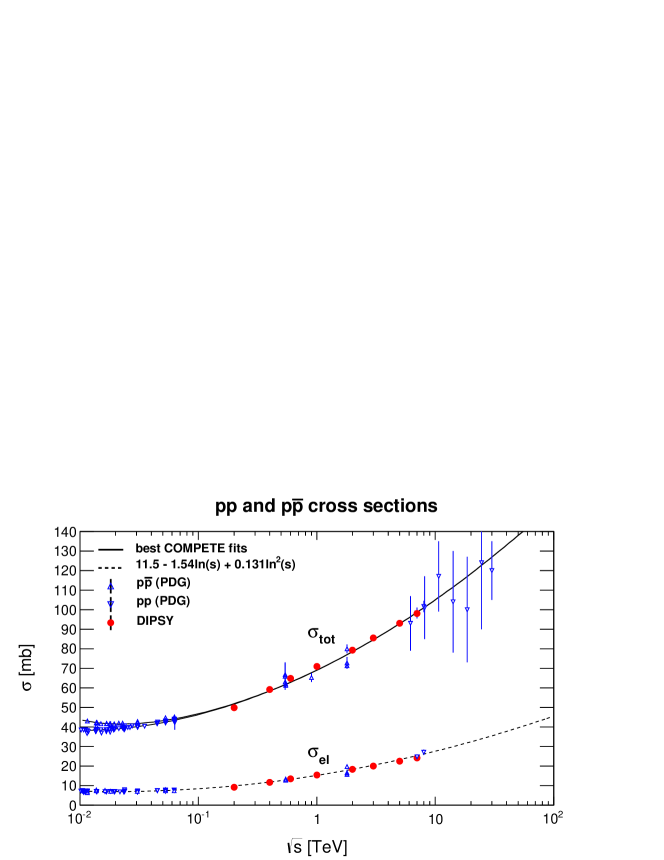
Figure 2: Total and elastic cross sections in $\mathrm{pp}$ and $\mathrm{p}\overline{\mathrm{p}}$ collisions plotted together with tuned DIPSY simulation results (red filled circles). The total cross section data (open triangles) are described by the best fit of the COMPETE collaboration [81] and the inelastic cross sections are also fitted by a phenomenological formula as shown in the figure.

4.1.2 $\mathrm{pPb}$ inelastic cross sections

Above the highest RHIC ion collision energy of $\sqrt{s_{NN}}=200$ GeV, in the region where DIPSY can be reliably applied, there are only a few heavy ion cross sections measured. One of them is the $\mathrm{pPb}$ total inelastic cross section for which the CMS [82] and LHCb [83] collaborations have presented preliminary results as shown in figure 3. The DIPSY results, shown by a solid line connecting the simulated points, agrees well with the data, as does the two additional theoretical calculations shown from the EPOS-LHC [85] and QGSJetII-04 [86] models.

The DIPSY results are mainly driven by the underlying geometrical description of the nucleus from the GLISSANDO parameterisation, as discussed in more detail in section 4.3.

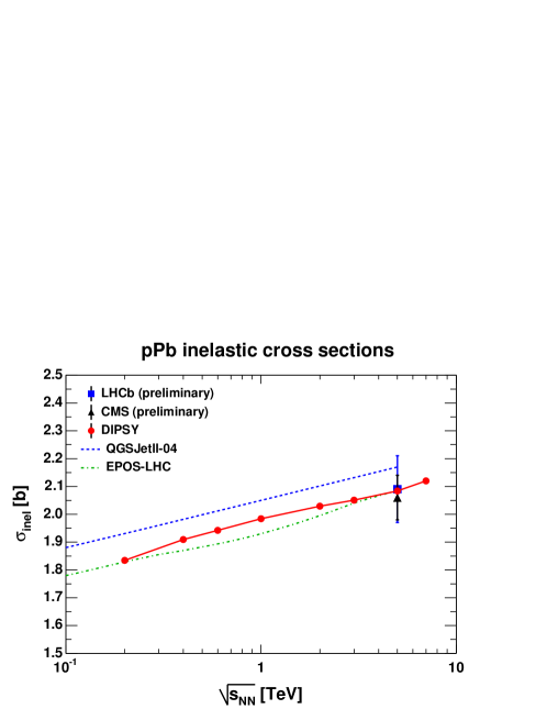
Figure 3: $\mathrm{pPb}$ inelastic cross sections recently measured by the CMS (black triangle) and the LHCb (blue square) collaborations. The solid line guides the eye for the DIPSY results starting from RHIC collision energies. The predictions of QGSJetII-04 [86] and EPOS-LHC [85] simulations are indicated by dotted and dashed lines, respectively.

4.2 Predictions for $\mathrm{p}A$ and $\gamma^{\star}A$ total cross sections

4.2.1 $\mathrm{p}A$ total cross sections

In figure 4 total cross sections calculated by DIPSY are shown for collisions of protons with different types of ions. Lead, copper and oxygen were selected to represent heavy, intermediate, and light ions to get an overview about the main characteristics of $\mathrm{p}A$ cross sections. We note that these cross sections grow more slowly with energy than the $\mathrm{pp}$ cross section in figure 2. This is more clearly seen in figure 5, where we show the ratio of the total $\mathrm{p}A$ cross section to the corresponding total $\mathrm{pp}$ cross section. For clarity, we here also normalise this ratio by the mass number, $A$, for the colliding ion. If the $NN$ cross section would be small, this ration should be one. The deviation from one, which is larger for the heavy lead nucleus and for higher energy, is thus a related to the average number of $NN$ collisions in a single $\mathrm{p}A$ event.

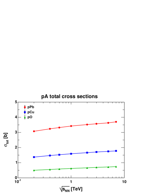
Figure 4: Total cross sections for $\mathrm{p}A$ collisions obtained from the DIPSY Monte Carlo model calculations. The results are shown as a function of the nucleon–nucleon centre-of-mass energy, covering a range from the upper RHIC energies to the available LHC energies.

For a completely black nucleus, the cross section is expected to scale with the area overlap for the two projectiles, i.e. $\propto(R_{A}+R_{p})^{2}$. Approximating $R_{A}\sim A^{1/3}R_{p}$ will thus lead to a scaling $\sim R_{p}^{2}(A^{1/3}+1)^{2}$. Figure 4 also shows the $\mathrm{p}A$ total cross sections scaled by $(A^{1/3}+1)^{2}$. We can here see that, as expected, this area scaling works better for heavy nuclei and high energy, when the black limit is approached. Analogously the contribution from volume effects $\propto A$ are more visible for smaller nuclei and lower energy.

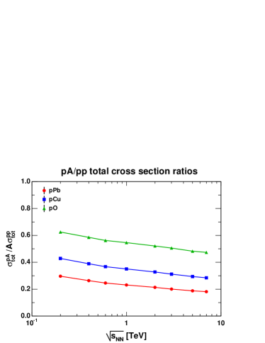
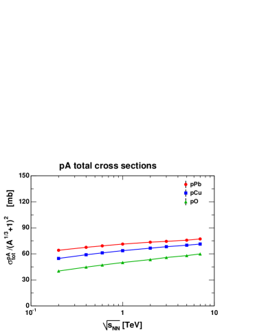
Figure 5: DIPSY predictions for the total $\mathrm{p}A$ cross sections scaled by $A\sigma_{\mathrm{tot}}^{pp}$ (left), and by $(A^{1/3}+1)^{2}$ (right). For the mass-number scaling the ratio for $\mathrm{pO}$ collisions closer to 1 than for $\mathrm{pPb}$ collisions, indicating, that volume effects are more important for lighter nuclei and at lower colliding energies, as far as the non-linear nuclear effects implemented in DIPSY are considered, while the opposite is found for the surface scaling.

4.2.2 $\gamma^{\star}A$ total cross sections

When a (virtual) photon fluctuates into a $q\bar{q}$ pair, it forms a colour dipole, which interacts with the nucleus in the same way as a dipole in a colliding proton. Thus it produces a dipole cascade, which is comparatively long-lived, and frozen during the interaction with the nucleus. In figures 6-8 we show the total cross section for $\gamma^{\star}A$ collisions in the energy range $\sqrt{s_{\gamma^{\star}A}}$ between 0.1 and 7 TeV, similar to the energy range studied above for $\mathrm{p}A$ collisions. Results are presented for photon virtualities $Q^{2}$ = 2.5, 5, 25 and 100 GeV² colliding with O, Cu, and Au nuclei. We also present the results after scaling with the $\gamma^{\star}\mathrm{p}$ cross section and the mass number $A$. We have used the parameters tuned to the $\mathrm{pp}$ cross sections in section 4.1, and we have checked that we reproduce data on $\gamma^{\star}\mathrm{p}$ cross sections to a reasonable degree. This means, however, that the $\gamma^{\star}A$ cross sections presented here should not be thought of as true precision predictions, and we will here only discuss the qualitative behavior of the cross sections and their ratios.

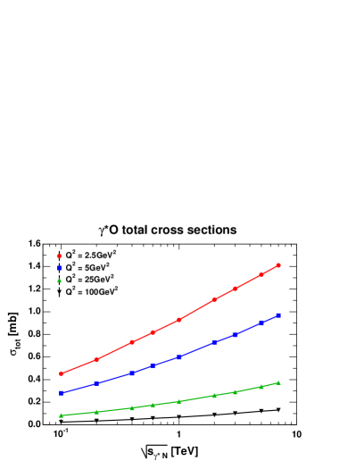
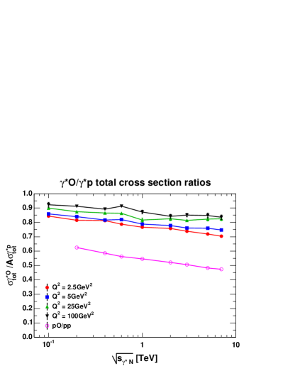
Figure 6: Left panel indicates DIPSY predictions for the total cross sections of $\gamma^{\star}\mathrm{O}$ reactions as a function of the photon virtuality $Q^{2}$ and the available energy $\sqrt{s_{\gamma^{\star}N}}$. The right panel compares these calculations to $\gamma^{\star}\mathrm{p}$ reactions, scaled also by the mass number $A$. For comparison we also show the ratio $\mathrm{pO}$/$\mathrm{pp}$.

We note that the dipole–nucleon cross section is suppressed compared to the $NN$ interaction, as an effect of colour transparency. Therefore the cross sections scale more closely with the volume $\sim A$ than with the area, as was the case for $\mathrm{p}A$ collisions. For the same reason it also grows with energy, approximately proportional to the $\gamma^{\star}\mathrm{p}$ cross section. As seen in the figures, this scaling is most clear for larger $Q^{2}$ and smaller $A$, while saturation effects become more noticeable for lower $Q^{2}$ and heavier nuclei.

The $\gamma^{\star}A$ cross section is also suppressed by the factor $\alpha_{EM}$ in the photon–quark coupling. Note that the cross sections are here measured in millibarn, instead of barn, which was used above for the $\mathrm{p}A$ cross sections. However, as the dipole state is frozen during the collision, this extra suppression has no effect on the scaling behaviour discussed here.

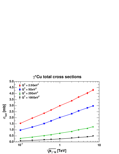
Figure 7: Same as figure 6 but for Cu nuclei.

Figure 7 indicates the results of a DIPSY simulation for the intermediately heavy Cu nuclei that can be compared in a straightforward way with the results shown on figure 6. From this comparison one can observe, that $\sigma_{\mathrm{tot}}^{\gamma^{\star}\mathrm{Cu}}/A\sigma_{\mathrm{tot}}^{\gamma^{\star}\mathrm{p}}<\sigma_{\mathrm{tot}}^{\gamma^{\star}\mathrm{O}}/A\sigma_{\mathrm{tot}}^{\gamma^{\star}\mathrm{p}}$ . This suggests that even for intermediately heavy nuclei such as Cu, it is more difficult for the dipoles to find a hole and to pass through these nuclei, as compared to lighter nuclei such as O.

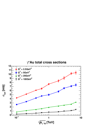
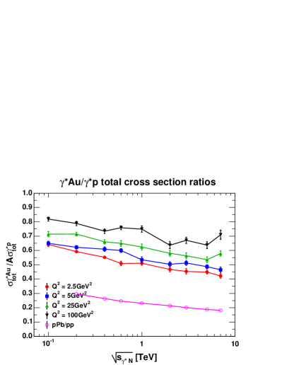
Figure 8: Same as figure 6 but for Au nuclei.

Figure 8 indicates that in $\gamma^{\star}\mathrm{Au}$ reactions the mass number or volume scaling is even worse approximation than in $\gamma^{\star}\mathrm{Cu}$ reactions. This indicates that for large nuclei and for large $\sqrt{s}$ the nuclei become asymptotically black even for a small dipole coming from a virtual photon, $\gamma^{\star}$. Nevertheless, when compared to calculations with similar centre-of-mass energies for $\mathrm{pPb}$ collisions, one can observe that virtual photons can pass through these large nuclei $\mathrm{Au}$ or $\mathrm{Pb}$ more easily as compared to the collision of protons with the same target.

4.3 Semi-inclusive $\mathrm{p}A$ cross sections and comparisons with Glauber models

Besides colour coherence effects, to be discussed in section 5.1, the most important feature of the DIPSY model for nucleus collisions is its treatment of correlations, and fluctuations, not only between the nucleons, but also inside the nucleons and between partons in different nucleons. To investigate the observable consequences of this we will in this section compare some results for semi-inclusive cross sections in DIPSY with those of standard Glauber calculations, where mainly fluctuations in the positions of nucleons and short range nuclear correlations between nucleons are considered.

In figure 9 we present DIPSY predictions for the inelastic, non-diffractive cross sections for $\mathrm{p}A$ collisions as a function of collision energy, comparing to a Glauber calculation using the black disc with the same nucleon distribution (see section 3.1) as input. Clearly the results are quite similar with differences only at the percent level. However, if we look at total $\mathrm{p}A$ cross sections in figure 10, the differences are much larger, almost up to 30% for small nuclei and lower energies. The differences here are mainly in the way how fluctuations are treated.

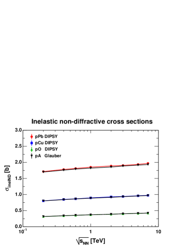
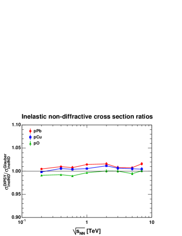
Figure 9: On the left panel Glauber Monte-Carlo and DIPSY calculations are compared for the $\sigma_{\mathrm{in,ND}}^{\mathrm{p}A}$ inelastic non-diffractive cross sections. In these calculations, the DIPSY results for $\sigma_{\mathrm{in,ND}}$ $\mathrm{pp}$ cross sections were used, as input, in the Glauber calculations. The Glauber Model MC results were obtained in the black-disc approach. The right panel shows the ratios of the DIPSY calculation to the Glauber Monte Carlo, indicating that the effects of correlations and fluctuations contribute to these variables on the typical 1% scale.

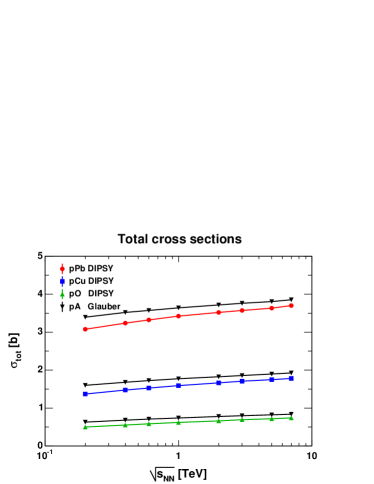
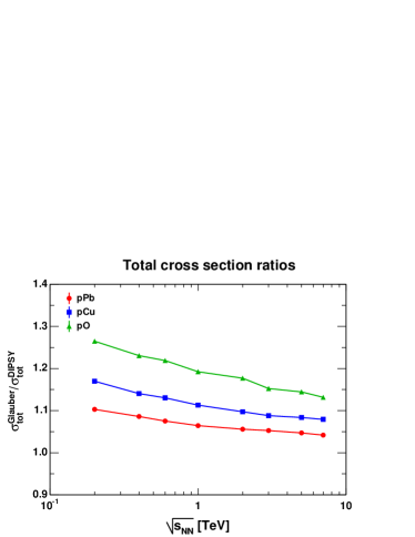
Figure 10: Left panel indicates a comparison of $\sigma_{\mathrm{tot}}^{\mathrm{p}A}$ total cross section calculations from DIPSY to the corresponding Glauber Model MC results, using the black-disc approach. For Glauber, the same $\sigma_{\mathrm{in,ND}}$ $\mathrm{pp}$ cross sections were used, as input, that DIPSY calculated. Right panel indicates the ratios of $\sigma_{\mathrm{tot}}^{\mathrm{p}A}$ total cross sections calculated by DIPSY to the Glauber Model MC in black-disc approach, indicating that although the inelastic cross sections are within 1% the same in the two approach, the predictions for the total cross section differ by a rather significant value that is about $20-30$% at RHIC energies and decreases to $10-15$% at LHC energies.

It should be noted that the input radius to the Glauber calculation is here taken from the inelastic, non-diffractive $\mathrm{pp}$ cross sections, c.f. eq. (9), using the value obtained from DIPSY. However, looking at eq. (10), it is clear that within the black disc approximation we could also have taken the total or elastic $\mathrm{pp}$ cross sections to define the input radius. In fact, if we had taken $\sigma^{\mathrm{pp}}_{\mathrm{tot}}=2\pi R^{2}$ to define the input radius, the difference w.r.t. DIPSY would be much smaller. On the other hand the differences for the inelastic, non-diffractive cross sections would then be larger.

As pointed out in section 3.2, the observables most sensitive to fluctuations are related to diffraction. For the black-disc Glauber calculations in eq. (10), the $\mathrm{pp}$ diffractive cross section is zero. For $\mathrm{p}A$ collisions, however, the Glauber calculation will result in a diffractive component, which is then entirely related to the fluctuations in the nucleon distribution within the nucleus. This can also be thought of as the elastic scattering of the proton projectile with one or more of the nucleons, resulting in a diffractive excitation of the nucleus. It is therefore interesting to compare this to DIPSY, where more fluctuations are taken into account.

Model	DIPSY		Black disc		Black disc		Black disc		Grey disc
			($\sigma_{\mathrm{tot}}$)		($\sigma_{\mathrm{in}}$)		($\sigma_{\mathrm{in,ND}}$)		($\sigma_{\mathrm{tot}},\sigma_{\mathrm{el}}$)
$\sqrt{s_{NN}}$ (TeV)	5	10	5	10	5	10	5	10	5	10
$\sigma_{\mathrm{tot}}$ (b)	$3.54$	$3.62$	$3.50$	$3.58$	$3.88$	$3.95$	$3.73$	$3.80$	$3.69$	$3.77$
$\sigma_{\mathrm{in}}$ (b)	$2.04$	$2.07$	$1.95$	$1.98$	$2.14$	$2.17$	$2.06$	$2.09$	$2.07$	$2.11$
$\sigma_{\mathrm{in,ND}}$ (b)	$1.89$	$1.92$	$1.75$	$1.79$	$1.94$	$1.98$	$1.86$	$1.90$	$1.84$	$1.89$
$\sigma_{\mathrm{el}}$ (b)	$1.51$	$1.55$	$1.55$	$1.60$	$1.73$	$1.78$	$1.66$	$1.70$	$1.62$	$1.66$
$\sigma_{\mathrm{SD,A}}$ (b)	$0.085$	$0.086$	$0.198$	$0.192$	$0.204$	$0.198$	$0.200$	$0.195$	$0.083$	$0.085$
$\sigma_{\mathrm{SD,p}}$ (b)	$0.023$	$0.024$	-	-	-	-	-	-	-	-
$\sigma_{\mathrm{DD}}$ (b)	$0.038$	$0.038$	-	-	-	-	-	-	$0.142$	$0.137$
$\sigma_{\mathrm{el*}}$ (b)	$1.59$	$1.64$	$1.75$	$1.79$	$1.94$	$1.98$	$1.86$	$1.90$	$1.70$	$1.75$
$\sigma_{\mathrm{el*}}/\sigma_{\mathrm{in}}$	$0.78$	$0.79$	$0.90$	$0.90$	$0.91$	$0.91$	$0.90$	$0.91$	$0.82$	$0.83$
$\sigma_{\mathrm{in,ND}}/\sigma_{\mathrm{tot}}$	$0.53$	$0.53$	$0.50$	$0.50$	$0.50$	$0.50$	$0.50$	$0.50$	$0.50$	$0.50$

Table 1: DIPSY predictions for different (semi-) inclusive $\mathrm{pPb}$ cross sections (given in units of barns) at LHC energies ($\sqrt{s^{NN}}=$ 5 and 10 TeV) compared to different Glauber calculations. The input radius to the black disc calculations were given by $\pi R^{2}=\sigma^{\mathrm{pp}}_{\mathrm{tot}}/2$, $\sigma^{\mathrm{pp}}_{\mathrm{in,ND}}$, and $\sigma^{\mathrm{pp}}_{\mathrm{in}}$. For the Grey disc both $\sigma^{\mathrm{pp}}_{\mathrm{tot}}$ and $\sigma^{\mathrm{pp}}_{\mathrm{el}}$ were used (see eq. (11)). In all cases using these $\mathrm{pp}$ cross sections obtained from DIPSY. The cross sections shown are the total ($\sigma_{\mathrm{tot}}$), the inelastic including diffractive excitation ($\sigma_{\mathrm{in}}$), the inelastic non-diffractive ($\sigma_{\mathrm{in,ND}}$), the elastic ($\sigma_{\mathrm{el}}$), the single diffractive excitation of the nucleus ($\sigma_{\mathrm{SD,A}}$) and proton ($\sigma_{\mathrm{SD,p}}$), the double diffractive excitation ($\sigma_{\mathrm{DD}}$), and the quasi-elastic scattering ($\sigma_{\mathrm{el*}}$ in eq. (13)). Also shown are the cross section ratios, $\sigma_{\mathrm{el*}}/\sigma_{\mathrm{in}}$ and $\sigma_{\mathrm{in,ND}}/\sigma_{\mathrm{tot}}$. The statistical uncertainty in the calculations are below a percent, except for the diffractive excitation cross sections, where the uncertainty is around 3%.

In table 1 we present predictions from DIPSY for different (semi-) inclusive $\mathrm{pPb}$ cross sections at LHC energies ($\sqrt{s^{NN}}\approx 5$ and 10 TeV) compared to different Glauber calculations. The input for the black disc radii were taken from the $\mathrm{pp}$ cross sections calculated by DIPSY, and for all cross sections we find a trivial increase as the radius becomes larger ($\sigma^{\mathrm{pp}}_{\mathrm{tot}}/2<\sigma^{\mathrm{pp}}_{\mathrm{in,ND}}<\sigma^{\mathrm{pp}}_{\mathrm{in}}$). As noted before the inelastic, non-diffractive cross section is close to DIPSY, when using the $\mathrm{pp}$ inelastic, non-diffractive cross section for the black-disc radius. We note, however, that the predicted cross sections for the diffractive dissociation of the nucleus are quite insensitive to the input radius, and are for a black disc in all three cases much larger than the predictions from DIPSY. This effect also shows up in the quasi-elastic cross sections (c.f. section 3.2). The reason for this can be found in the fact that all black-disc calculations over-estimate the elastic nucleon–nucleon cross section, resulting in a larger probability to quasi-elastically excite the nucleus.

It is therefore interesting to also compare with a grey-disc Glauber calculation (c.f. eq. (11)), where both the elastic and the total $NN$ cross sections are set to the same as in DIPSY. In table 1 we see that the nucleus dissociation cross section in this case is very close to DIPSY. However, since the elastic $\mathrm{pPb}$ cross section comes out slightly larger than in DIPSY, also the quasi-elastic cross section is larger.

The inelastic $\mathrm{pPb}$ cross section has already been measured at LHC [82, 83], and there is also a possibility to measure the quasi-elastic cross section using e.g. the TOTEM experiment. In table 1 we also present predictions for the ratio between these cross sections, as one may expect that some systematic uncertainties in the experimental measurements (e.g. uncertainties in luminosity) may cancel in such a ratio.

For completeness we also show in table 1 the DIPSY results for single diffractive excitation of the proton, which is absent in all the Glauber calculations, and the double diffraction cross section, which is zero in the black disc approximations. Finally, we note that the ratio $\sigma_{\mathrm{in,ND}}/\sigma_{\mathrm{tot}}$ by construction is one half in the Glauber calculations (see eqs. (10) and (11)), while in DIPSY, the ratio is slightly higher.

5 Discussion

5.1 Saturation effects

Colour reconnection (swing) is one of the nuclear effects introduced in the Lund Dipole Cascade Model DIPSY. Such a swing may take place if dipoles of the same colour are close enough in a longer chain of dipoles, or, if the colour configuration of two different chains allows for a colour reconnection. This reconnection may happen with certain probability discussed in section 2 in such a way that preferably smaller dipole chains are formed, possibly giving rise to chains forming small closed loops. Smaller dipoles reduce the interaction probability and hence result in smaller cross sections. This feature effectively corresponds to a gluon saturation effect, as mentioned already at the description of the DIPSY model in section 2.

In this section, we quantify the magnitude of the swing effect for electron–nucleus (more precisely virtual photon–nucleus) and proton–nucleus collisions. In particular, we switch on and off the inter-nucleon swings. However, it is important to note that we keep the intra-nucleon swings turned on so that the values of the total and elastic $\mathrm{pp}$ cross sections remain the same as indicated in figure 2.

It is well known that Gribov corrections to multiple diffractive scattering [21] are typically on the $10-15$% scale and in principle they take into account the fluctuating size of the projectile when evaluating, for example, the total cross section of proton–nucleus or deuteron–nucleus collisions. In this picture, it is important to consider that the projectile itself has a fluctuating size, and when it is in a small size configuration, it can pass through the nucleus easier. Hence the total $\mathrm{p}A$ cross section is typically reduced when the Gribov correction is taken into account. Intra-nucleon swings may increase the fluctuations in the size of the nucleon, and are hence related to these Gribov corrections. The inter-nucleon swing mechanism is an additional, new effect, that may decrease the probability of the interaction further, reducing the impact of large colour dipole configurations even further.

In figure 11 the total cross sections with and without inter-nucleon swing are compared for $\gamma^{\star}\mathrm{O}$, $\gamma^{\star}\mathrm{Au}$, $\mathrm{pO}$ and $\mathrm{pPb}$ reactions. As the number of possible swings will increase with the number of dipoles, and hence with the collision energy, one might assume that the effects of the inter-nucleon swing would also increase with energy, however from figure 11 it is clear that the energy dependence is practically flat. From this we can conclude that the main effect comes from reconnections related to the initial dipoles of the nucleons. For a virtual photon probe we find the largest effect for a heavy nucleus (over 10% for $\gamma^{\star}\mathrm{Au}$), which is natural, since here we have more nucleons overlapping in impact-parameter space. For a proton projectile, however, the effects overall as well as the differences between nuclei are smaller, since for central collisions (where the overlap is largest) at these energies, the nucleus is already effectively “black”, while the same nucleus is much more transparent for a virtual photon probe.

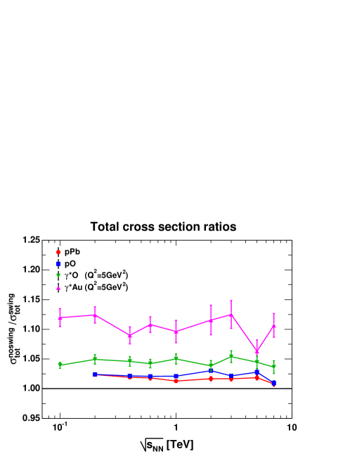
Figure 11: Total cross section ratios for $\mathrm{pPb}$ and $\mathrm{pO}$ reactions, as well as for $\gamma^{\star}\mathrm{O}$ and $\gamma^{\star}\mathrm{Au}$, with inter-nucleon of swing mechanism switched off as compared to on.

5.2 Frame (in)dependence as a function of $\sigma^{\mathrm{pp}}_{\mathrm{tot}}$

In this sub-section we demonstrate how can one minimise the dependence of the results of the DIPSY model on the frame chosen as reference frame for the simulation. The reason for this discussion is that the Lund Cascade Model DIPSY is not formulated in an entirely boost-invariant manner, yet, so the simulation results depend slightly on the Lorentz-frame chosen as a reference frame.

The results presented in section 4 are obtained using the $NN$ (or $\gamma^{\star}N$) centre-of-mass frame, with parameters tuned to $\mathrm{pp}$ total and elastic cross sections in this frame. The screening effects in interactions with nuclei are most sensitive to the cross section for the individual $NN$ collisions. Therefore, although the result depends on the frame used when the parameter values are fixed, as is shown in the left panel of figure 12, the result is insensitive to the frame if the parameters are tuned, in the same frame, to $\mathrm{pp}$ cross section data. This is illustrated on the right panel of figure 12, which shows $\sigma_{\mathrm{tot}}^{\mathrm{pPb}}/A\sigma_{\mathrm{tot}}^{\mathrm{pp}}$ as function of the $\mathrm{pp}$ total cross section.

This way the error due to the frame dependence is reduced to a level of about 1% or less, as illustrated in the right panel of figure 12, which negligible as compared to the $10-15$% size of the dynamical swing effect that we explored in the previous sub-section.

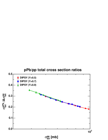
Figure 12: Left panel indicates the frame dependence of the normalised $\sigma_{\mathrm{tot}}^{\mathrm{pPb}}/A\sigma_{\mathrm{tot}}^{\mathrm{pp}}$ total cross section ratios calculated in three different frames,given by $y_{frame}=(1-Y)\cdot y_{p}+Y\cdot y_{A}$, with $Y=0.5,\,0.7$, and 0.9, as a function of the centre-of-mass energy. We see that even these normalised ratios have a frame dependence of about 25%. The right panel, however, illustrates that most of the frame dependence enters through the frame dependence of the total $\mathrm{pp}$ cross section: if these values are correctly tuned to the measurements in the frame of the calculation, the results (with less than 1% error) become approximately frame independent.

6 Conclusions

Analyses of collective behaviour from final state properties in $AA$ collisions depend crucially on the assumptions about the initial state, obtained from parton–parton interactions. This initial state is sensitive to all possible correlations, fluctuations, and colour interference effects between the partons within a nucleon as well as in different nucleons. To draw stable conclusions, it is therefore important to have a good understanding of this initial state. It has often been suggested that studies of $\mathrm{p}A$ collisions, as intermediate between $AA$ and $\mathrm{pp}$ collisions, will be of great help here.

In this paper we will investigate the properties of a high energy nucleus via studies of total, elastic, and quasi-elastic cross sections in $\mathrm{p}A$ and $\gamma^{\star}A$ collisions, as these observables depend only upon the initial states, but are insensitive to any collective effects in the final state interactions. The Lund Dipole Cascade model DIPSY offers special possibilities to study the evolution of gluons inside hadrons and nuclei, including effects of unitarization at small $x$, interference, correlations, and fluctuations. The model is based on BFKL evolution, including essential non-leading effects, saturation, and colour interference effects. It reproduces successfully total, elastic, and diffractive cross sections in $\mathrm{pp}$ collisions and DIS, within the energy range from RHIC to LHC for $\mathrm{pp}$ collisions and the HERA range for DIS, and it can be directly generalised to study collisions with nuclei.

The general features of the results are, as expected, that in $\mathrm{p}A$ interactions the centre is rather black, which means that the cross section approximately scales with the area $(R_{A}+R_{p})^{2}\sim R_{p}^{2}(A^{1/3}+1)^{2}$. In $\gamma^{\star}A$ collisions the nucleus is much more transparent, in particular for high $Q^{2}$ and lighter nuclei. The cross sections therefore here scale approximately with $A$, but behaves somewhat more similar to $\mathrm{p}A$ for smaller $Q^{2}$ and/or larger $A$ and higher energy. As a particularly interesting effect we note that colour coherence effects between gluons in different nucleons in the nucleus, can reduce the $\gamma^{\star}\mathrm{Au}$ cross section by about 10%. These results underline the importance of future electron–ion collider experiments to study the initial partonic state of highly energetic nuclei.

To study the more subtle effects related to colour coherence and fluctuations, we make comparisons with Glauber calculations. We here see that the interesting effects show up in the relative size of the total, elastic, diffractive, and quasi-elastic cross sections. We point out that both the experimental and the theoretical accuracy will be higher for these ratios than for the individual cross sections.

Finally we note that the DIPSY program is also able to produce exclusive hadronic final states in $\mathrm{pp}$ collisions [32]. The extension of this to also model final states of collisions involving heavy ions is certainly feasible, but the effects of the extremely crowded partonic environment in $\mathrm{p}A$ and $AA$ are not trivial and must be modelled with great care. Progress towards understanding string fragmentation in a dense environment has already been made in [87], but the full picture of the final states in the DIPSY dipole model is yet to come.

Appendix A Appendix. The Good–Walker formalism for diffractive excitation.

Diffraction is normally interpreted as elastic scattering driven by absorption. If the absorption probability in Born approximation is given by $2F$, then rescattering exponentiates in impact parameter space, giving the unitarized absorption probability

$$P_{abs}=d\sigma_{\mathrm{in}}/d^{2}b=1-e^{-2F}.$$ (14)

We define the elastic amplitude, $T$, via the relation $S\equiv 1-T$, which makes $T$ real. The optical theorem, $T=(1/2)(T^{2}+P_{abs})$, then gives the following result for the amplitude and the elastic and total cross sections:

$$T = 1-e^{-F}$$ (15)

$$d\sigma_{\mathrm{el}}/d^{2}b = (1-e^{-F})^{2}$$ (16)

$$d\sigma_{\mathrm{tot}}/d^{2}b = 2(1-e^{-F}).$$ (17)

For a projectile with a substructure, the mass eigenstates can differ from the eigenstates of diffraction, i.e. states with a specific absorption probability [22]. Call the diffractive eigenstates $\Phi_{n}$, with elastic scattering amplitudes $T_{n}$. The mass eigenstates $\Psi_{k}$ are linear combinations of the states $\Phi_{n}$:

$$\Psi_{k}=\sum_{n}c_{kn}\Phi_{n}\,\,\,\,\,\,(\mathrm{with}\,\,\Psi_{in}=\Psi_{1}).$$ (18)

The elastic scattering amplitude is given by

$$\langle\Psi_{1}|T|\Psi_{1}\rangle=\sum c_{1n}^{2}T_{n}=\langle T\rangle,$$ (19)

and the elastic cross section

$$d\sigma_{\mathrm{el}}/d^{2}b=(\sum c_{1n}^{2}T_{n})^{2}=\langle T\rangle^{2}.$$ (20)

The amplitude for diffractive transition to the mass eigenstate $\Psi_{k}$ is given by

$$\langle\Psi_{k}|T|\Psi_{1}\rangle=\sum_{n}c_{kn}T_{n}c_{1n},$$ (21)

which gives a total diffractive cross section (including elastic scattering)

$$d\sigma_{\mathrm{diff}}/d^{2}b=\sum_{k}\langle\Psi_{1}|T|\Psi_{k}\rangle\langle\Psi_{k}|T|\Psi_{1}\rangle=\langle T^{2}\rangle.$$ (22)

Consequently the cross section for diffractive excitation is given by the fluctuations:

$$d\sigma_{\mathrm{D}}/d^{2}b=d\sigma_{\mathrm{diff}}/d^{2}b-d\sigma_{\mathrm{el}}/d^{2}b=\langle T^{2}\rangle-\langle T\rangle^{2}.$$ (23)

If also the target has a substructure, it is possible to have either single excitation of the projectile, of the target, or double diffractive excitation, with cross sections given in section 2.1.

References

- [1] Z. Fodor and S. Katz, “Lattice determination of the critical point of QCD at finite T and mu,” JHEP 0203 (2002) 014, arXiv:hep-lat/0106002 [hep-lat].
- [2] Z. Fodor and S. Katz, “Critical point of QCD at finite T and mu, lattice results for physical quark masses,” JHEP 0404 (2004) 050, arXiv:hep-lat/0402006 [hep-lat].
- [3] BRAHMS Collaboration Collaboration, I. Arsene et al., “Quark gluon plasma and color glass condensate at RHIC? The Perspective from the BRAHMS experiment,” Nucl.Phys. A757 (2005) 1–27, arXiv:nucl-ex/0410020 [nucl-ex].
- [4] PHENIX Collaboration, K. Adcox et al., “Formation of dense partonic matter in relativistic nucleus-nucleus collisions at RHIC: Experimental evaluation by the PHENIX collaboration,” Nucl.Phys. A757 (2005) 184–283, arXiv:nucl-ex/0410003 [nucl-ex].
- [5] PHOBOS Collaboration, B. Back, M. Baker, M. Ballintijn, D. Barton, B. Becker, et al., “The PHOBOS perspective on discoveries at RHIC,” Nucl.Phys. A757 (2005) 28–101, arXiv:nucl-ex/0410022 [nucl-ex].
- [6] STAR Collaboration, J. Adams et al., “Experimental and theoretical challenges in the search for the quark gluon plasma: The STAR Collaboration’s critical assessment of the evidence from RHIC collisions,” Nucl.Phys. A757 (2005) 102–183, arXiv:nucl-ex/0501009 [nucl-ex].
- [7] ALICE Collaboration, J. F. Grosse-Oetringhaus, “Overview of ALICE Results at Quark Matter 2014,” Nucl.Phys. A931 (2014) 22–31, arXiv:1408.0414 [nucl-ex].
- [8] ATLAS Collaboration, A. Milov, “Particle production and long-range correlations in p+Pb collisions with the ATLAS detector,” arXiv:1403.5738 [nucl-ex].
- [9] CMS Collaboration, R. Granier de Cassagnac, “CMS heavy-ion overview,” Nucl.Phys. A931 (2014) 13–21.
- [10] PHENIX Collaboration, A. Adare et al., “Beam-energy and system-size dependence of the space-time extent of the pion emission source produced in heavy ion collisions,” arXiv:1410.2559 [nucl-ex].
- [11] R. A. Lacey, “Observation of the critical end point in the phase diagram for hot and dense nuclear matter,” arXiv:1411.7931 [nucl-ex].
- [12] A. M. Sickles, “Experimental Results on Collisions at RHIC and the LHC,” Nucl.Phys. A931 (2014) 63–72, arXiv:1408.0220 [nucl-ex].
- [13] EHS/NA22 Collaboration, N. Agababyan et al., “Estimation of hydrodynamical model parameters from the invariant spectrum and the Bose-Einstein correlations of pi- mesons produced in (pi+ / K+)p interactions at 250-G V/c,” Phys.Lett. B422 (1998) 359–368, arXiv:hep-ex/9711009 [hep-ex].
- [14] UA5 Collaboration, G. Alner et al., “Kaon Production in Reactions at a Center-of-mass Energy of 540-GeV,” Nucl.Phys. B258 (1985) 505.
- [15] CMS Collaboration, V. Khachatryan et al., “Strange Particle Production in Collisions at and 7 TeV,” JHEP 1105 (2011) 064, arXiv:1102.4282 [hep-ex].
- [16] STAR Collaboration, J. Adams et al., “Identified hadron spectra at large transverse momentum in p+p and d+Au collisions at s(NN)**(1/2) = 200-GeV,” Phys.Lett. B637 (2006) 161–169, arXiv:nucl-ex/0601033 [nucl-ex].
- [17] A. Ortiz Velasquez, P. Christiansen, E. Cuautle Flores, I. Maldonado Cervantes, and G. Paić, “Color Reconnection and Flowlike Patterns in Collisions,” Phys.Rev.Lett. 111 no.~4, (2013) 042001, arXiv:1303.6326 [hep-ph].
- [18] CMS Collaboration, V. Khachatryan et al., “Observation of Long-Range Near-Side Angular Correlations in Proton-Proton Collisions at the LHC,” JHEP 1009 (2010) 091, arXiv:1009.4122 [hep-ex].
- [19] R. Glauber, “Cross-sections in deuterium at high-energies,” Phys.Rev. 100 (1955) 242–248.
- [20] R. Glauber and G. Matthiae, “High-energy scattering of protons by nuclei,” Nucl.Phys. B21 (1970) 135–157.
- [21] V. Gribov, “Glauber corrections and the interaction between high-energy hadrons and nuclei,” Sov.Phys.JETP 29 (1969) 483–487.
- [22] M. Good and W. Walker, “Diffraction disssociation of beam particles,” Phys.Rev. 120 (1960) 1857–1860.
- [23] H. I. Miettinen and J. Pumplin, “Diffraction Scattering and the Parton Structure of Hadrons,” Phys.Rev. D18 (1978) 1696.
- [24] A. Bialas, M. Bleszynski, and W. Czyz, “Multiplicity Distributions in Nucleus-Nucleus Collisions at High-Energies,” Nucl.Phys. B111 (1976) 461.
- [25] W. Broniowski, M. Rybczynski, and P. Bozek, “GLISSANDO: Glauber initial-state simulation and more..,” Comput.Phys.Commun. 180 (2009) 69–83, arXiv:0710.5731 [nucl-th].
- [26] M. Rybczynski, G. Stefanek, W. Broniowski, and P. Bozek, “GLISSANDO 2: GLauber Initial-State Simulation AND mOre…, ver. 2,” Comput.Phys.Commun. 185 (2014) 1759–1772, arXiv:1310.5475 [nucl-th].
- [27] M. Alvioli, H.-J. Drescher, and M. Strikman, “A Monte Carlo generator of nucleon configurations in complex nuclei including Nucleon-Nucleon correlations,” Phys.Lett. B680 (2009) 225–230, arXiv:0905.2670 [nucl-th].
- [28] M. Alvioli and M. Strikman, “Color fluctuation effects in proton-nucleus collisions,” Phys.Lett. B722 (2013) 347–354, arXiv:1301.0728 [hep-ph].
- [29] E. Avsar, G. Gustafson, and L. Lönnblad, “Energy conservation and saturation in small-x evolution,” JHEP 07 (2005) 062, arXiv:hep-ph/0503181.
- [30] E. Avsar, G. Gustafson, and L. Lönnblad, “Small-x dipole evolution beyond the large-N(c) limit,” JHEP 01 (2007) 012, arXiv:hep-ph/0610157.
- [31] E. Avsar, G. Gustafson, and L. Lönnblad, “Diifractive excitation in DIS and collisions,” JHEP 12 (2007) 012, arXiv:0709.1368 [hep-ph].
- [32] C. Flensburg, G. Gustafson, and L. Lönnblad, “Inclusive and Exclusive observables from dipoles in high energy collisions,” arXiv:1103.4321 [hep-ph].
- [33] C. Flensburg, “Heavy ion inital states from DIPSY,” Prog.Theor.Phys.Suppl. 193 (2012) 172–175.
- [34] T. Sjöstrand, S. Ask, J. R. Christiansen, R. Corke, N. Desai, et al., “An Introduction to PYTHIA 8.2,” Comput.Phys.Commun. 191 (2015) 159–177, arXiv:1410.3012 [hep-ph].
- [35] M. Bahr, S. Gieseke, M. Gigg, D. Grellscheid, K. Hamilton, et al., “Herwig++ Physics and Manual,” Eur.Phys.J. C58 (2008) 639–707, arXiv:0803.0883 [hep-ph].
- [36] P. Aurenche, F. W. Bopp, R. Engel, D. Pertermann, J. Ranft, et al., “DTUJET-93: Sampling inelastic proton proton and anti-proton - proton collisions according to the two component dual parton model,” Comput.Phys.Commun. 83 (1994) 107–123, arXiv:hep-ph/9402351 [hep-ph].
- [37] T. Pierog, I. Karpenko, J. Katzy, E. Yatsenko, and K. Werner, “EPOS LHC : test of collective hadronization with LHC data,” arXiv:1306.0121 [hep-ph].
- [38] L. Gribov, E. Levin, and M. Ryskin, “Semihard Processes in QCD,” Phys.Rept. 100 (1983) 1–150.
- [39] L. D. McLerran and R. Venugopalan, “Computing quark and gluon distribution functions for very large nuclei,” Phys.Rev. D49 (1994) 2233–2241, arXiv:hep-ph/9309289 [hep-ph].
- [40] I. Balitsky, “Operator expansion for high-energy scattering,” Nucl.Phys. B463 (1996) 99–160, arXiv:hep-ph/9509348 [hep-ph].
- [41] Y. V. Kovchegov, “Small x F(2) structure function of a nucleus including multiple pomeron exchanges,” Phys.Rev. D60 (1999) 034008, arXiv:hep-ph/9901281 [hep-ph].
- [42] C. Flensburg, G. Gustafson, and L. Lönnblad, “Elastic and quasi-elastic and scattering in the Dipole Model,” Eur. Phys. J. C60 (2009) 233–247, arXiv:0807.0325 [hep-ph].
- [43] A. H. Mueller, “Soft gluons in the infinite momentum wave function and the BFKL pomeron,” Nucl. Phys. B415 (1994) 373–385.
- [44] A. H. Mueller and B. Patel, “Single and double BFKL pomeron exchange and a dipole picture of high-energy hard processes,” Nucl. Phys. B425 (1994) 471–488, arXiv:hep-ph/9403256.
- [45] A. H. Mueller, “Unitarity and the BFKL pomeron,” Nucl. Phys. B437 (1995) 107–126, arXiv:hep-ph/9408245.
- [46] E. A. Kuraev, L. N. Lipatov, and V. S. Fadin, “The Pomeranchuk Singularity in Nonabelian Gauge Theories,” Sov. Phys. JETP 45 (1977) 199–204.
- [47] I. Balitsky and L. Lipatov, “The Pomeranchuk Singularity in Quantum Chromodynamics,” Sov.J.Nucl.Phys. 28 (1978) 822–829.
- [48] G. Gustafson, L. Lönnblad, and G. Miu, “Hadronic collisions in the linked dipole chain model,” Phys.Rev. D67 (2003) 034020, arXiv:hep-ph/0209186 [hep-ph].
- [49] G. Salam, “OEDIPUS: Onium evolution, dipole interaction and perturbative unitarization simulation,” Comput.Phys.Commun. 105 (1997) 62–76, arXiv:hep-ph/9601220 [hep-ph].
- [50] G. Gustafson, “The Relation between the Good-Walker and Triple-Regge Formalisms for Diffractive Excitation,” Phys.Lett. B718 (2013) 1054–1057, arXiv:1206.1733 [hep-ph].
- [51] C. Flensburg and G. Gustafson, “Fluctuations, Saturation, and Diffractive Excitation in High Energy Collisions,” JHEP 1010 (2010) 014, arXiv:1004.5502 [hep-ph].
- [52] V. S. Fadin and L. N. Lipatov, “BFKL pomeron in the next-to-leading approximation,” Phys. Lett. B429 (1998) 127–134, hep-ph/9802290.
- [53] M. Ciafaloni and G. Camici, “Energy scale(s) and next-to-leading BFKL equation,” Phys. Lett. B430 (1998) 349–354, hep-ph/9803389.
- [54] G. P. Salam, “An introduction to leading and next-to-leading BFKL,” Acta Phys. Polon. B30 (1999) 3679–3705, arXiv:hep-ph/9910492.
- [55] M. Ciafaloni, “Coherence Effects in Initial Jets at Small q**2 / s,” Nucl.Phys. B296 (1988) 49.
- [56] B. Andersson, G. Gustafson, and J. Samuelsson, “The Linked dipole chain model for DIS,” Nucl.Phys. B467 (1996) 443–478.
- [57] J. Kwiecinski, A. D. Martin, and P. J. Sutton, “Constraints on gluon evolution at small x,” Z. Phys. C71 (1996) 585–594, arXiv:hep-ph/9602320.
- [58] A. H. Mueller and G. Salam, “Large multiplicity fluctuations and saturation effects in onium collisions,” Nucl.Phys. B475 (1996) 293–320, arXiv:hep-ph/9605302 [hep-ph].
- [59] T. Sjostrand, S. Mrenna, and P. Z. Skands, “PYTHIA 6.4 Physics and Manual,” JHEP 0605 (2006) 026, arXiv:hep-ph/0603175 [hep-ph].
- [60] C. Flensburg, G. Gustafson, L. Lönnblad, and A. Ster, “Correlations in double parton distributions at small x,” JHEP 1106 (2011) 066, arXiv:1103.4320 [hep-ph].
- [61] S. Catani, F. Fiorani, and G. Marchesini, “QCD Coherence in Initial State Radiation,” Phys.Lett. B234 (1990) 339.
- [62] C. Flensburg, G. Gustafson, and L. Lönnblad, “Exclusive final states in diffractive excitation,” JHEP 1212 (2012) 115, arXiv:1210.2407 [hep-ph].
- [63] E. Avsar and G. Gustafson, “Geometric scaling and QCD dynamics in DIS,” JHEP 0704 (2007) 067, arXiv:hep-ph/0702087 [HEP-PH].
- [64] M. L. Miller, K. Reygers, S. J. Sanders, and P. Steinberg, “Glauber modeling in high energy nuclear collisions,” Ann.Rev.Nucl.Part.Sci. 57 (2007) 205–243, arXiv:nucl-ex/0701025 [nucl-ex].
- [65] J.-P. Blaizot, W. Broniowski, and J.-Y. Ollitrault, “Correlations in the Monte Carlo Glauber model,” Phys.Rev. C90 no.~3, (2014) 034906, arXiv:1405.3274 [nucl-th].
- [66] H. De Vries, C. W. De Jager, and C. De Vries, “Nuclear charge-density-distribution parameters from elastic electron scattering,” Atom. Data Nucl. Data Tabl. 36 (1987) 495–536.
- [67] M. Rybczynski and W. Broniowski, “Two-body nucleon-nucleon correlations in Glauber-like models,” Phys.Part.Nucl.Lett. 8 (2011) 992–994, arXiv:1012.5607 [nucl-th].
- [68] CDF Collaboration, F. Abe et al., “Measurement of single diffraction dissociation at GeV and 1800 GeV,” Phys.Rev. D50 (1994) 5535–5549.
- [69] H1 Collaboration, C. Adloff et al., “Inclusive measurement of diffractive deep inelastic ep scattering,” Z.Phys. C76 (1997) 613–629, arXiv:hep-ex/9708016 [hep-ex].
- [70] ZEUS Collaboration, S. Chekanov et al., “Study of deep inelastic inclusive and diffractive scattering with the ZEUS forward plug calorimeter,” Nucl.Phys. B713 (2005) 3–80, arXiv:hep-ex/0501060 [hep-ex].
- [71] B. Blaettel, G. Baym, L. Frankfurt, H. Heiselberg, and M. Strikman, “Hadronic cross-section fluctuations,” Phys.Rev. D47 (1993) 2761–2772.
- [72] V. Guzey and M. Strikman, “Proton-nucleus scattering and cross section fluctuations at RHIC and LHC,” Phys.Lett. B633 (2006) 245–252, arXiv:hep-ph/0505088 [hep-ph].
- [73] The ATLAS collaboration, “Measurement of the centrality dependence of the charged particle pseudorapidity distribution in proton-lead collisions at TeV with the ATLAS detector,”.
- [74] L.-K. Ding and E. Stenlund, “A MONTE CARLO FOR NUCLEAR COLLISION GEOMETRY,” Comput.Phys.Commun. 59 (1990) 313–318.
- [75] H. Pi, “An Event generator for interactions between hadrons and nuclei: FRITIOF version 7.0,” Comput.Phys.Commun. 71 (1992) 173–192.
- [76] A. Accardi, J. Albacete, M. Anselmino, N. Armesto, E. Aschenauer, et al., “Electron Ion Collider: The Next QCD Frontier - Understanding the glue that binds us all,” arXiv:1212.1701 [nucl-ex].
- [77] T. Burton, “The eRHIC Project,” EPJ Web Conf. 70 (2014) 00064.
- [78] TOTEM Collaboration, G. Antchev et al., “Luminosity-Independent Measurement of the Proton-Proton Total Cross Section at TeV,” Phys.Rev.Lett. 111 no.~1, (2013) 012001.
- [79] TOTEM Collaboration, G. Antchev et al., “Measurement of proton-proton elastic scattering and total cross-section at S**(1/2) = 7-TeV,” Europhys.Lett. 101 (2013) 21002.
- [80] Particle Data Group Collaboration, J. Beringer et al., “Review of Particle Physics (RPP),” Phys.Rev. D86 (2012) 010001.
- [81] J. R. Cudell et al., “Benchmarks for the Forward Observables at RHIC, the Tevatron-Run II, and the LHC,” Phys. Rev. Lett. 89 (2002) 201801.
- [82] CMS Collaboration, C. Collaboration, “Measurement of the inelastic pPb cross section at 5.02 TeV,” CMS-PAS-FSQ-13-006 (2013) , CERN Document Server:1637959.
- [83] LHCb Collaboration, “First analysis of the Pb pilot run data with LHCb,” LHCb-CONF-2012-034, CERN-LHCb-CONF-2012-034 (2012) , CERN Document Server:1490049.
- [84] ALICE Collaboration, B. Abelev et al., “Pseudorapidity density of charged particles in + Pb collisions at TeV,” Phys.Rev.Lett. 110 no.~3, (2013) 032301, arXiv:1210.3615 [nucl-ex].
- [85] K. Werner, F. M. Liu, and T. Pierog, “Parton ladder splitting and the rapidity dependence of transverse momentum spectra in deuteron-gold collisions at RHIC,” Phys. Rev. C 74 (2006) 044902, arXiv:hep-ph/0506232.
- [86] S. Ostapchenko, “Air shower calculations with QGSJET-II: Effects of Pomeron loops,” Nucl. Phys. Proc. Suppl. 196 (2009) 90.
- [87] C. Bierlich, G. Gustafson, L. Lönnblad, and A. Tarasov, “Effects of Overlapping Strings in pp Collisions,” JHEP 1503 (2015) 148, arXiv:1412.6259 [hep-ph].