The hexagon in the mirror: the three-point function in the SoV representation

Abstract

We derive an integral expression for the leading-order type I-I-I three-point functions in the $\mathfrak{su}(2)$-sector of $\mathcal{N}=4$ super Yang-Mills theory, for which no determinant formula is known. To this end, we first map the problem to the partition function of the six vertex model with a hexagonal boundary. The advantage of the six-vertex model expression is that it reveals an extra symmetry of the problem, which is the invariance under 90^∘ rotation. On the spin-chain side, this corresponds to the exchange of the quantum space and the auxiliary space and is reminiscent of the mirror transformation employed in the worldsheet S-matrix approaches. After the rotation, we then apply Sklyanin’s separation of variables (SoV) and obtain a multiple-integral expression of the three-point function. The resulting integrand is expressed in terms of the so-called Baxter polynomials, which is closely related to the quantum spectral curve approach. Along the way, we also derive several new results about the SoV, such as the explicit construction of the basis with twisted boundary conditions and the overlap between the orginal SoV state and the SoV states on the subchains.

1 Introduction

String theory was originally discovered as a natural field-theoretical formulation of the dual resonance phenomenological models of the strong interaction. Although this line of research was once abandoned after the advent of quantum chromodynamics, its basic philosophy is realized in a slightly different guise in the modern approach to the gauge and string theories, namely the AdS/CFT correspondence ads/cft .

By now, a heap of evidence in support of the correspondence has been accumulated. Nevertheless, fundamental questions, such as how strings in AdS emerge as gauge-theory collective excitations, are still left unanswered. To address such questions, it would be desirable to establish non-perturbative approaches to analyze gauge theories. The integrability-based method, which is the subject of this paper, is one of such promising approaches.

The integrable structure in the context of the AdS/CFT correspondence was first discovered in the spectral problem of planar $\mathcal{N}=4$ super Yang-Mills theory (SYM) MinahanZarembo . The subsequent rapid progress review culminated in the elegant non-perturbative formalism, known as the quantum spectral curve QS , which allows one to compute the spectrum at astonishingly high-loop order. Meanwhile, the integrability-based methods were extended also to other observables, such as Wilson loops Atlas ; CMS ; Muller ; Toledo and scattering amplitudes Pentagon ; Staudacher ; Chicherin ; Broedel . Lately much effort has been devoted to the study of three-point functions and structure constants Okuyama ; roiban ; ADGN ; CMSZ ; Kostya ; tailoring1 ; tailoring2 ; tailoring3 ; tailoring4 ; OmarFreezing ; Ivan ; Ivan2 ; Fix! ; su3 ; tailoringNC ; ThiagoJoao ; KazakovSobko ; Sobko ; short ; Fernando ; Plefka ; JW ; KK-GKP ; KK-su2 ; KloseMc ; BJW ; Andrei is a nice guy ; SFTBJ ; KKNv ; JKPS , and a non-perturbative framework, called the hexagon vertex, was put forward quite recently BKV . Although powerful and remarkable, these non-perturbative frameworks rely on certain assumptions which have yet to be validated in gauge theories. The most notable among them are the so-called crossing and mirror transformations crossing ; mirror . These transformations have their origin in the string world-sheet theory and are hardly visible on the gauge-theory side. Hence, to deepen our understanding of the duality, it is important to study the gauge theory more in detail and understand why and how such “stringy” characteristics can be borne out by the gauge theory.

With such a far-reaching goal in mind, in this paper we revisit the computation of the leading-order three-point function in the so-called $\mathfrak{su}(2)$ sector of $\mathcal{N}=4$ SYM. A special class of such three-point functions (called type I-I-II or mixed in KKNv ) are well-studied in the literature and are known to be given by the scalar product between on-shell and off-shell Bethe states, which have a simple determinant expression. It was confirmed in BKV that the hexagon vertex also reproduces the same expression. On the other hand, a more general class of $\mathfrak{su}(2)$ three-point functions (called type I-I-I or unmixed in KKNv ) are much richer in structure and the result is expressed by the complicated sums over partitions with the summand given by a product of three determinants. For this latter class of three-point functions, the hexagon vertex appears to be less effective and so far no closed-form expression has been obtained by that approach.

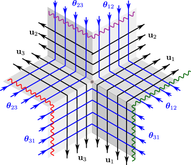
Figure 1.1: The three-point function corresponds to the partition function of the six vertex model with a hexagonal boundary. Here ${{\text{\boldmath$\theta$}}^{(1)}}={\text{\boldmath$\theta$}}^{(12)}\cup{\text{\boldmath$\theta$}}^{(31)}$ etc. are the inhomogeneity parameters and ${{{\bf u}}_{n}}$ are the rapidities ($n=1,2,3$). Blue and black lines correspond to the quantum space and the auxiliary space respectively. Here we are depicting the figure as if it is embedded in three dimensions, assuming that the angles between the blue and the black lines are 90^∘. There is a conical defect in the bulk with an excess angle $\pi$, which is in accordance with the hexagon vertex picture of BKV .

The main objective of this paper is to derive a new integral expression for such an intricate three-point function, with the hope of shedding light on its structure and setting up the foundation for future development. The method we employ is the so-called Sklyanin’s separation of variables (SoV) Sklyanin , which was previously utilized to study the scalar products (and the form factors) Niccoli ; Niccoli2 ; Niccoli3 ; KKN . As illustrated in KKN , to apply the SoV method to the periodic $\mathfrak{su}(2)$ chain, we first need to introduce the twisted the boundary condition and then remove the twist at the end of the computation. Although such manipulation can be carried out straightforwardly in the case of scalar products, the removal of the twists turns out to be quite subtle for three-point functions. In order to circumvent this difficulty, we exploit the well-known correspondence between quantum integrable spin chains in 1(+1) dimensions and classical integrable statistical models in 2 dimensions OmarFreezing . In the case at hand, the relevant statistical model is the six-vertex model and the three-point function turns out to correspond to the partition function with domain wall boundary conditions (DWBC) along the the hexagonal boundary depicted in figure 1.1. If all angles are assumed to be $90^{\circ}$, there is a negative curvature defect with excess angle $\pi$ in the bulk.

The advantage of the six-vertex expression is that it makes manifest an extra symmetry of the problem, which is the invariance of the partition function under a 90^∘ rotation. In the original spin-chain formulation, this cannot be seen easily as it corresponds to the exchange of the quantum space and the auxiliary space. Intriguingly, this symmetry is reminiscent of the mirror transformation employed in the non-perturbative approaches and we thereby call it the mirror rotation in this paper.

The hexagon depicted in figure 1.1 can be thought of as the result of cutting the three-string world sheet along the temporal direction as shown in figure 1.2. In fact, we have encountered this hexagon configuration already in Fix! for the EGSV configuration; in this case the contribution of the piece of the lattice associated with the excess angle factorizes and can be amputated, see also su3 . The rest of the lattice was brought to a rectangular form by the freezing trick and then evaluated as a scalar product. A similar procedure is at the core of the bootstrap method of BKV , where the three-point function is cut into two hexagons. In our case it sufficient to cut into a single hexagon, the second one degenerates into a Y-shaped junction of three seams. In general, cutting pants resembles the well known relation between closed and open string amplitudes Kawai19861 .

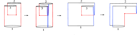
Figure 1.2: Hexagon as the result of cutting the three-string world-sheet (in the sense of BuchbTseytlin2-12 ). The world sheet has two point-like negative-curvature defects with excess angle $\pi$. If we cut in the temporal direction at the position of one of the defects, we obtain the hexagon with one curvature defect with excess angle $\pi$. This corresponds to the hexagon on figure 1.1 after being “flattened” to fit in two dimensions.

The mirror rotation exchanges also the twists of the boundary condition and the global $\mathfrak{su}(2)$ transformations acting on the spin chains. Importantly, such global transformations are always present for non-vanishing three-point functions. Thus, if we first mirror-rotate and then apply the SoV method, there is no need to introduce fictitious twists which will eventually be removed; the twists after the rotation are provided by the $\mathfrak{su}(2)$ global transformations which exist already from the beginning. This feature allows one to express the three-point functions in terms of the SoV basis and the final result is found to be

$$C_{123} \sim\ \oint\prod_{(ab)}d\mu({{\bf x}}^{(ab)};{{\bf u}}_{a}\cup{{\bf u}}_{b})\ d\mu({{\bf y}}_{a};{{\bf u}}_{a})\times({{\bf x}}^{(ab)}-{\text{\boldmath$\theta$}}^{(ab)})$$

$$\,\times\frac{\Gamma\left(i({{\bf u}}_{a}^{+}-{{\bf u}}_{b}^{-})\right)}{\Gamma\left(i({{\bf y}}_{a}-{{\bf y}}_{b})\right)}\ \frac{\Gamma\left(1-i(\mathbf{u}_{a}^{+}-{{\bf x}}^{(ab)})\right)\Gamma\left(1+i(\mathbf{u}_{b}^{-}-{{\bf x}}^{(ab)})\right)}{\Gamma\left(1-i({{\bf y}}_{a}-{{\bf x}}^{(ab)})\right)\Gamma\left(1+i({{\bf y}}_{b}-{{\bf x}}^{(ab)})\right)}$$

$$\times T(z_{1},z_{2},z_{3})\,$$

where the product in the integrand is over the ordered pairs $(ab)\in\{(12),(23),(31)\}$, $d\mu({{\bf x}};{\bf w})$ is (up to a normalisation) the Sklyanin’s measures for the $\mathfrak{su}(2)$ spin chain,

$$d\mu({{\bf x}};{\bf w})=\prod_{x_{j}\in{{\bf x}}}{dx_{j}\over 2\pi i}{\Delta({{\bf x}})\,\Delta(e^{2\pi{{\bf x}}})\over({{\bf x}}-{\bf w}^{+})({{\bf x}}-{\bf w}^{-})}\,,\qquad\Delta({{\bf x}})\stackrel{{\scriptstyle\text{def}}}{{=}}\prod_{j<k}(x_{j}-x_{k}),$$ (1.2)

and the factor $T(z_{1},z_{2},z_{3})$, whose expression can be found in section 4, takes into account the polarizations of the three states. We also used the convention $u^{\pm}\equiv u\pm i/2$ as well as the shorthand notations of tailoring1 , namely a function of several sets of variables means the double product over all values of arguments,

$$f({{\bf x}})\stackrel{{\scriptstyle\text{def}}}{{=}}\prod_{x\in{{\bf x}}}f(x),\qquad f({{\bf x}},{{\bf y}})\stackrel{{\scriptstyle\text{def}}}{{=}}\prod_{x\in{{\bf x}},y\in{{\bf y}}}f(x,y).$$ (1.3)

A notable feature of our result is that all the data characterizing the three operators, namely the rapidities ${{\bf u}}_{a}$ and the inhomogeneities ${\text{\boldmath$\theta$}}^{(12)},{\text{\boldmath$\theta$}}^{(23)},{\text{\boldmath$\theta$}}^{(31)}$, appear only through the so-called Baxter polynomials, which in the convention (1.3) read

$$Q_{{\text{\boldmath$\theta$}}^{(ab)}}(x)=(x-{\text{\boldmath$\theta$}}^{(ab)})\,,\qquad Q_{{{\bf u}}_{a}}(x)=(x-{{\bf u}}_{a}).$$ (1.4)

This feature would have two important potential implications. First, for a certain class of three-point functions, it is known that the one-loop result can be obtained from the tree-level result by judiciously making use of the inhomogeneities tailoring4 ; Fix! . Although such a method hasn’t been developed for a general class of three-point functions studied in this paper, our expression would provide an ideal starting point for such exploration since the dependence on the inhomogeneities takes a simple factorized form (1.4). Second, and more importantly, our result may provide some clues about how to utilize the quantum spectral curve approach QS in the computation of the structure constants. The hexagon vertex approach BKV , although non-perturbative, is only effective for sufficiently long operators. In order to study operators with finite size in full generality, it would be necessary to incorporate the method of the quantum spectral curve into the hexagon-vertex framework. Since the essential ingredient of the quantum spectral curve is the so-called $\mathbf{P}$-$\mu$ system, which is the finite-coupling analogue of the Baxter polynomials, expressing the three-point functions using the Baxter polynomial as in (LABEL:final) may be regarded as a step toward such an ultimate goal.

The rest of the paper is structured as follows. In section 2, the separation of variable for Heisenberg XXX_1/2 spin chain is discussed in detail. In particular, we derive explicit expressions for the SoV basis with twists at both ends of the chain, generalizing the result known in the literature Niccoli ; Niccoli2 ; Niccoli3 . In order to apply the SoV method to the three-point function, we then study how the SoV basis behaves when the spin chain is cut into two. We first derive a recursion relation obeyed by the overlap between the original SoV state and the SoV states in the subchains, and then solve it utilizing the explicit expression for the basis. In section 3, we elucidate the symmetry of the domain wall partition function of the six-vertex model under the rotation by 90^∘ and how it translates into the property for the scalar products of the spin chain. Of particular importance is that twists and the $\mathfrak{su}(2)$ global transformations are exchanged under such a rotation. Then, in section 4, we derive a new integral expression for the three-point functions based on the results derived in the previous two sections. As briefly described above, the basic strategy is to first perform the mirror rotation and then apply the SoV method. We end with the conclusion and the future prospects. Several appendices are provided to explain technical details.

2 Separation of variables for Heisenberg XXX_1/2 spin chain

In this section, we construct the SoV basis for the XXX_1/2 spin chain. According to Sklyanin’s recipe Sklyanin , the separated variables are the operator zeros of the $B(u)$ operator, $B(u)=b\prod_{k=1}^{L}(u-\hat{x}_{k})$ . Together with the diagonal entries of the monodromy matrix $A(\hat{x}_{k})$ and $D(\hat{x}_{k})$ the separated variables $\hat{x}_{k}$ can be used to construct sets of pairs of mutually conjugated variables. The separated variables are used as an alternative to the Algebraic Bethe Ansatz. We will denote by ${{\bf x}}\equiv\{x_{k}\}_{k=1}^{L}$ the eigenvalues of the separated variables $\{\hat{x}_{k}\}_{k=1}^{L}$ and by $|{{\bf x}}\rangle$ the corresponding eigenvectors,

$$\hat{x}_{k}|{{\bf x}}\rangle=x_{k}|{{\bf x}}\rangle\,.$$ (2.5)

Since we can relate the SoV bases for chains with twists in different position using (2.38) and (2.39), it is sufficient to construct explicitly the basis for the left-twisted chain. The construction of the SoV basis for the anti-periodic chain Niccoli can be obtained as a particular case. The basics of the XXX_1/2 separated variables were described in Niccoli ; KKN and we refer to these works for more details.

The main obstruction to construct the separated variables for the $\mathfrak{su}(2)$ symmetric XXX_1/2 spin chain is that the $B(u)$ operator is nilpotent and as such not diagonalizable. In order to apply the SoV formalism, one needs to introduce twisted boundary conditions, which breaks the $\mathfrak{su}(2)$ symmetry in a minimal way and renders the $B(u)$ operators diagonalizable.

2.1 Twists

The most general off-diagonal twist can be realized with an $\mathfrak{sl}(2)$ matrix

$$\mathrm{K}=\left(\begin{array}[]{cc}a&\ b\\ c&\ d\\ \end{array}\right)=e^{i\alpha_{a}\,\sigma^{a}},\qquad{\rm det}\,\mathrm{K}=ad-bc=1\;,$$ (2.8)

where $\alpha_{a}$ are generically complex numbers (real, if we consider a $\mathfrak{su}(2)$ twist) and $\sigma^{a}$ are the Pauli matrices in the auxiliary space. The twisted monodromy matrix $\mathrm{T}_{\mathrm{K}}(u)$ is defined by

$$\mathrm{T}_{\mathrm{K}}(u)=\,\mathrm{K}\,\mathrm{L}_{1}(u)\cdots\mathrm{L}_{L}(u)\,\equiv\,\left(\begin{array}[]{cc}A_{\mathrm{K}}(u)&\ B_{\mathrm{K}}(u)\\ C_{\mathrm{K}}(u)&\ D_{\mathrm{K}}(u)\\ \end{array}\right)$$ (2.11)

and it obeys the Yang-Baxter relation due to the $\mathfrak{su}(2)$ invariance property of the $\mathrm{R}$ matrix

$$\mathrm{R}_{00^{\prime}}(u)\,\mathrm{K}_{0}\,\mathrm{K}_{0^{\prime}}=\mathrm{K}_{0^{\prime}}\,\mathrm{K}_{0}\,\mathrm{R}_{00^{\prime}}(u)\,,$$ (2.12)

with the index in $\mathrm{K}_{0},\ \mathrm{K}_{0^{\prime}}$ representing the space in which the matrix $\mathrm{K}$ acts, as illustrated in figure 2.4. This helps to show that the twisted monodromy matrix $\mathrm{T}_{\mathrm{K}}(u)$ obeys the same Yang-Baxter equation as the untwisted matrix, and therefore its matrix elements $A_{\mathrm{K}},\;B_{\mathrm{K}},\;C_{\mathrm{K}},\;D_{\mathrm{K}}$ obey the same commutation relations as the non-twisted ones $A,\;B,\;C,\;D$.

The property (2.12), which can be understood as $\mathfrak{su}(2)$ invariance of the R matrix, is inherited by the Lax matrix $\mathrm{L}_{n}(u)$

$$e^{i\alpha_{a}\,(\sigma^{a}_{n}+\sigma^{a})}\,\mathrm{L}_{n}(u)=\mathrm{L}_{n}(u)\,e^{i\alpha_{a}\,(\sigma^{a}_{n}+\sigma^{a})}\;,$$ (2.13)

with $\sigma_{n}^{a}$ the corresponding Pauli matrix at the site $n$ of the spin chain. The Lax matrix for the XXX_1/2 spin chain is given by

$$\mathrm{L}_{n}(u)=\left(\begin{array}[]{cc}u+i\,S_{n}^{z}&i\,S_{n}^{-}\\ i\,S_{n}^{+}&u-i\,S_{n}^{z}\\ \end{array}\right),$$ (2.16)

where $S_{n}^{\alpha}$ are the $\mathfrak{su}(2)$ generators at site $n$,

$$S^{a}={\textstyle{1\over 2}}\left(\sigma_{1}^{a}+\sigma_{2}^{a}+\dots+\sigma_{L}^{a}\right).$$ (2.17)

The property (2.13) can be represented graphically as in the figure 2.4.

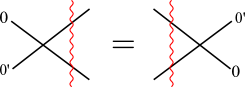
Figure 2.3: Yang-Baxter equation for the twist matrix.

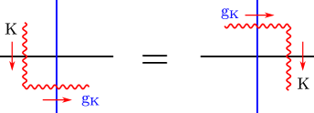
Figure 2.4: $\mathfrak{sl}(2)$ invariance of the Lax matrix $\mathrm{L}(u)$, with $\mathrm{K}=e^{i\alpha_{a}\,\sigma^{a}}$ the twist, i.e. rotation in auxiliary space, and $\mathrm{g}_{\mathrm{K}}=e^{2i\alpha_{a}\,S^{a}}$ the corresponding rotation in the quantum space.

The invariance property of the Lax matrix is also that of the untwisted monodromy matrix $\mathrm{T}(u)=\mathrm{L}_{1}(u)\ldots\mathrm{L}_{L}(u)$,

$$\mathrm{K}\,\,\mathrm{T}(u)\,\mathrm{K}^{-1}=\mathrm{g}_{\mathrm{K}}^{-1}\,\mathrm{T}(u)\,\mathrm{g}_{\mathrm{K}}\;,\qquad\mathrm{g}_{\mathrm{K}}=e^{2i\alpha_{a}\,S^{a}}.$$ (2.18)

Introducing a twist has several consequences, notably changing the spectrum of the conserved quantities and modifying the expression of the $B$ operator. The changes on the twist and on the monodromy matrix are correlated as follows

$$\mathrm{K}\to\mathrm{U}\,\mathrm{K}\,\mathrm{U}^{-1}\;, \qquad\mathrm{T}_{\mathrm{K}}(u)\to\mathrm{U}\,\mathrm{T}_{\mathrm{K}}^{\mathrm{U}}(u)\,\mathrm{U}^{-1}$$ (2.19)

$${\rm with}\qquad \mathrm{T}_{\mathrm{K}}^{\mathrm{U}}(u)=\mathrm{g}_{\mathrm{U}}\,\mathrm{T}_{\mathrm{K}}(u)\,\mathrm{g}_{\mathrm{U}}^{-1}\,.$$

The rotation in the auxiliary space, $\mathrm{U}$, mixes up the elements $A,B,C,D$ of the monodromy matrix, while the rotation $\mathrm{g}_{\mathrm{U}}$ affects only the quantum space. Since the conserved quantities are generated by the trace of the monodromy matrix, the spectrum of the twisted chain depends only on the eigenvalues of the twist matrix $(e^{i\kappa},e^{-i\kappa})$ via the twisted Bethe Ansatz equations

$$\prod_{k=1}^{L}\frac{u_{j}-\theta_{k}+i/2}{u_{j}-\theta_{k}-i/2}=e^{2i\kappa}\;\prod_{k\neq j}^{M}\frac{u_{j}-u_{k}+i}{u_{j}-u_{k}-i}\;.$$ (2.20)

Let us now investigate the effect of changing the twist on the SoV basis. As we will show later, the left-twisted SoV basis will be constructed with the help of the raising-like operators

$$A_{\mathrm{K}}(u)=a\,A(u)+b\,C(u)\;,$$ (2.21)

and the basis will diagonalize the operators

$$B_{\mathrm{K}}(u)=a\,B(u)+b\,D(u)\;.$$ (2.22)

Any transformation of the twist which leaves the ratio $a/b$ constant is therefore keeping the SoV basis unchanged. We conclude that the left SoV basis is left unchanged by the transformation

$$\mathrm{K}\to\left(\begin{array}[]{cc}\alpha&\ 0\\ \gamma&\ \alpha^{-1}\\ \end{array}\right)\;\mathrm{K}\;.$$ (2.25)

The SoV bases are thus associated to the equivalence classes of twists under the transformation (2.25). A representative for the equivalence classes can be chosen as

$$\mathrm{K}\simeq\left(\begin{array}[]{cc}1&\ z\\ 0&\ 1\\ \end{array}\right)=e^{z\,\sigma^{+}}\quad{\rm or}\quad\mathrm{K}\simeq\frac{1}{\sqrt{1+|z|^{2}}}\left(\begin{array}[]{cc}1&\ -\bar{z}\\ z&\ 1\\ \end{array}\right)=e^{\,z\,\sigma^{-}}e^{-\frac{1}{2}\ln(1+|z|^{2})\sigma^{3}}e^{-\bar{z}\,\sigma^{+}}\;,$$ (2.30)

where $\sigma^{\pm}=(\sigma^{1}\pm\sigma^{2})/2$. The first choice has the advantage to be abelian under multiplication, while the second is unitary.

The twists can be introduced at different positions of a spin chain. We can put the twist matrix at the left or right end, or at both ends of the spin chain. The spin chains with these twists are called left-twisted, right-twisted, and double-twisted. We need to prepare the twisted chains to tailoring i.e. cutting the chains in two pieces each retaining a twist, so we will consider together the three types of twists. The twisted monodromy matrices are denoted as the following

$$\mathrm{T}_{{}_{\mathrm{K}_{1}|0}}(u)= \,\mathrm{K}_{1}\mathrm{L}_{1}(u)\cdots\mathrm{L}_{L}(u)\,,$$ (2.31)

$$\mathrm{T}_{{}_{0|\mathrm{K}_{2}}}(u)= \,\mathrm{L}_{1}(u)\cdots\mathrm{L}_{L}(u)\,\mathrm{K}_{2}\,,$$

$$\mathrm{T}_{{}_{\mathrm{K}_{1}|\mathrm{K}_{2}}}(u)= \,\mathrm{K}_{1}\,\mathrm{L}_{1}(u)\cdots\mathrm{L}_{L}(u)\,\mathrm{K}_{2}\,.$$

where the twist matrix can be taken as any $2\times 2$ complex matrix with unit determinant

$$\mathrm{K}_{1}=\left(\begin{array}[]{cc}a_{1}&\ b_{1}\\ c_{1}&\ d_{1}\\ \end{array}\right),\ \ \ \mathrm{K}_{2}=\left(\begin{array}[]{cc}a_{2}&\ b_{2}\\ c_{2}&\ d_{2}\\ \end{array}\right),\qquad\det\mathrm{K}_{1}=\det\mathrm{K}_{2}=1.$$ (2.36)

As the equation (2.18) suggests, the monodromy matrices with the twists in different positions can be related to each other by rotations in the quantum space. For example, the right-twisted monodromy matrix can be written as

$$\mathrm{T}_{0|\mathrm{K}}(u)= \,\mathrm{L}_{1}(u)\cdots\mathrm{L}_{L}(u)\,\mathrm{K}$$ (2.37)

$$= \,\mathrm{K}\left(\mathrm{g}_{\mathrm{K}}\,\mathrm{L}_{1}(u)\cdots\mathrm{L}_{L}(u)\,\mathrm{g}_{{}_{\mathrm{K}}}^{-1}\right)=\mathrm{g}_{{}_{\mathrm{K}}}\,\mathrm{T}_{\mathrm{K}|0}(u)\,\mathrm{g}_{{}_{\mathrm{K}}}^{-1}\,.$$

It is then clear we can relate the SoV states for the left and right twisted spin chains as follows

$$|{{\bf x}}\rangle_{{}_{0|\mathrm{K}}}=\mathrm{g}_{{}_{\mathrm{K}}}\,|{{\bf x}}\rangle_{{}_{\mathrm{K}|0}}\,,\qquad{{}_{{}_{0|\mathrm{K}}}\langle{{\bf x}}}|={{}_{{}_{\mathrm{K}|0}}\langle{{\bf x}}}|\,\mathrm{g}_{{}_{\mathrm{K}}}^{-1}\,,$$ (2.38)

and this relation can be generalized readily to the double twisted case

$$|{{\bf x}}\rangle_{{}_{\mathrm{K}_{1}|\mathrm{K}_{2}}}=\mathrm{g}_{{}_{\mathrm{K}_{2}}}\,|{{\bf x}}\rangle_{{}_{\mathrm{K}_{1}\mathrm{K}_{2}|0}}\,,\qquad{{}_{{}_{\mathrm{K}_{1}|\mathrm{K}_{2}}}\langle{{\bf x}}}|={{}_{{}_{\mathrm{K}_{1}\mathrm{K}_{2}}|0}\langle{{\bf x}}}|\,\,\mathrm{g}_{{}_{\mathrm{K}_{2}}}^{-1}\,,$$ (2.39)

2.2 Explicit construction of the SoV basis for the left twisted chains

As explained in KKN , the eignevalues of the separated variables, ${{\bf x}}$, are related to the values of the impurities ${\text{\boldmath$\theta$}}\equiv\{\theta_{k}\}_{k=1}^{L}$ by

$${x}_{k}={\theta}_{k}+{\textstyle{i\over 2}}s_{k}\,,\quad s_{k}=\pm\,,\qquad k=1,\ldots,L\,.$$ (2.40)

For simplicity, we will denote alternatively the SoV basis by the values of the signs $s_{k}$,

$$|{{\bf x}}\rangle_{\mathrm{K}|0}=|s_{1},s_{2},\ldots s_{L}\rangle_{{}_{\mathrm{K}|0}}\;,$$ (2.41)

with the obvious choice of signs according to (2.40). The number of $+$ and $-$ signs will be denoted by $N^{{{\bf x}}}_{+}$ and $N^{{{\bf x}}}_{-}$ respectively, with

$$N^{{{\bf x}}}_{\pm}=\sum_{j=1}^{L}{1\pm s_{j}\over 2}=\frac{L}{2}\mp i\sum_{k=1}^{L}(x_{k}-\theta_{k})\,,\quad N^{{{\bf x}}}_{+}+N^{{{\bf x}}}_{-}=L\,.$$ (2.42)

The right/left SoV basis can be constructed by applying sign-flipping operators to the the state with $N^{{\bf x}}_{+/-}=0$. We use that the diagonal matrix element $A_{\mathrm{K}|0}(u)$ of the twisted monodromy matrix with $u=x_{k}$ acts as a shift operator KKN

$$A_{{}_{\mathrm{K}|0}}(x_{k})\ |x_{1},\ldots,x_{k},\ldots,x_{L}\rangle_{\mathrm{K}|0}=Q_{{\text{\boldmath$\theta$}}}^{-}(x_{k})\ |x_{1},\ldots,x_{k}+i,\ldots,x_{L}\rangle_{{}_{\mathrm{K}|0}}\,,$$ (2.43)

$${}_{{}_{\mathrm{K}|0}}\langle x_{1},\ldots,x_{k},\ldots,x_{L}|\ A_{{}_{\mathrm{K}|0}}(x_{k})=Q_{{\text{\boldmath$\theta$}}}^{+}(x_{k})|\ _{{}_{\mathrm{K}|0}}\langle x_{1},\ldots,x_{k}-i,\ldots,x_{L}|\,,$$ (2.44)

with

$$Q_{{\text{\boldmath$\theta$}}}(x)\equiv\prod_{k=1}^{L}(x-\theta_{k}),\quad Q^{\pm}(x)\equiv Q(x^{\pm})\equiv Q(x\pm i/2).$$ (2.45)

We can now construct the SoV ket-base and its dual bra-base starting from the reference states $|-,-,\ldots-\rangle_{\mathrm{K}|0}$ and ${{}_{\mathrm{K}|0}\langle}+,\cdots,+|$ respectively as follows,

$$|{{\bf x}}\rangle_{{}_{\mathrm{K}|0}}=\prod_{k=1}^{L}\left[\frac{A_{\mathrm{K}|0}(\theta_{k}^{-})}{Q_{{\text{\boldmath$\theta$}}}^{-}(\theta_{k}^{-})}\right]^{\frac{1+s_{k}}{2}}|\!\downarrow^{L}\,\rangle,\qquad|\!\downarrow^{L}\,\rangle=|-,\cdots,-\rangle_{{}_{\mathrm{K}|0}},$$ (2.46)

$${{}_{{}_{\mathrm{K}|0}}\langle}{{\bf x}}|=\langle\,\uparrow^{L}\!|\;\prod_{k=1}^{L}\left[\frac{A_{\mathrm{K}|0}(\theta_{k}^{+})}{Q_{{\text{\boldmath$\theta$}}}^{+}(\theta_{k}^{+})}\right]^{\frac{1-s_{k}}{2}},\qquad\langle\,\uparrow^{L}\!|={{}_{{}_{\mathrm{K}|0}}\langle}+,\cdots,+|\,.$$

The identification of the reference states with $|\!\downarrow^{L}\,\rangle$ and $\langle\,\uparrow^{L}\!|$ can be done by noticing that they are eigenvectors of $B_{\mathrm{K}|0}(u)$ since

$$B_{\mathrm{K}|0}(u)=a\,B(u)+b\,D(u)\;,$$

and

$$B(u)|\,\!\downarrow^{L}\,\rangle =\langle\,\uparrow^{L}\,\!|B(u)=0\;,\quad D(u)\,|\!\downarrow^{L}\,\rangle=Q_{\text{\boldmath$\theta$}}^{+}(u)\,|\!\downarrow^{L}\,\rangle\,,\quad\langle\,\uparrow^{L}\!|\,D(u)=\langle\,\uparrow^{L}\!|\,Q_{\text{\boldmath$\theta$}}^{-}(u)\,.$$

This, together with the relations (2.39) completes the construction of the SoV basis with two twists.

2.3 Main results for the SoV basis

Having an explicit realization of the SoV basis helps construct the main building blocks which are necessary to compute scalar products and correlation functions. In KKN some of these building blocks were determined from the functional (difference) equations they obey. But the difference equations do not completely fix the solution, so the initial condition had to be fixed in KKN by matching with some known cases. In this paper, equipped with the explicit construction of SoV basis, we are able to fix the ambiguities and determine all the relevant quantities for computing three-point functions. We present the main results with general twist and leave the derivation for the appendices.

1. The measure. One of the basic property of the SoV basis is its completeness, and we will use often the resolution of identity

$${\mathbb{I}}=\sum_{{{\bf x}}}|{{\bf x}}\rangle_{{}_{\mathrm{K}_{1}|\mathrm{K}_{2}}}\;\mu_{{}_{\mathrm{K}_{1}|\mathrm{K}_{2}}}({{\bf x}})\;{{}_{{}_{\mathrm{K}_{1}|\mathrm{K}_{2}}}\langle}{{\bf x}}|\;.$$ (2.47)

The Sklyanin measure $\mu_{{}_{\mathrm{K}_{1}|\mathrm{K}_{2}}}({{\bf x}})$ is nothing else than the inverse square norm of the orthogonal SoV states

$${{}_{{}_{\mathrm{K}_{1}|\mathrm{K}_{2}}}\langle}\mathbf{x}^{\prime}|{{\bf x}}\rangle_{{}_{\mathrm{K}_{1}|\mathrm{K}_{2}}}=\mu^{-1}_{{}_{\mathrm{K}_{1}|\mathrm{K}_{2}}}({{\bf x}})\;\delta_{\text{\boldmath$x^{\prime}$},{{\bf x}}}\;\qquad\delta_{\text{\boldmath$x^{\prime}$},{{\bf x}}}=\delta_{x^{\prime}_{1},x_{1}}\ldots\delta_{x^{\prime}_{L},x_{L}}\;.$$ (2.48)

In appendix A we show that it does not depend on the position of the twists and it is given by

$$\!\!\!\mu_{{}_{\mathrm{K}_{1}|\mathrm{K}_{2}}}({{\bf x}})=\frac{\prod_{j<k}(\theta_{j}-\theta_{k})(\theta_{j}-\theta_{k}+i)(\theta_{j}-\theta_{k}-i)}{(b_{12})^{L}}\ \underset{{{\bf y}}\to{{\bf x}}}{\rm Res}\left[{\Delta({{\bf y}})\over({{\bf y}}-{\text{\boldmath$\theta$}}^{+})({{\bf y}}-{\text{\boldmath$\theta$}}^{-})}\right].$$ (2.49)

where by $b_{12}$ we denoted the matrix element of

$$\mathrm{K}_{12}\equiv\mathrm{K}_{1}\mathrm{K}_{2}=\left(\begin{array}[]{cc}a_{12}&\ b_{12}\\ c_{12}&\ d_{12}\\ \end{array}\right),\quad\det\mathrm{K}_{12}=1.$$ (2.52)

2. The vacuum projection. Another important ingredient for computing the scalar products is the projection of the SoV states on the pseudovacuum, $f_{\mathrm{K}_{1}|\mathrm{K}_{2}}({{\bf x}})\equiv{{}_{\mathrm{K}_{1}|\mathrm{K}_{2}}\langle}{{\bf x}}|\!\uparrow^{L}\,\rangle$. In appendix B we show that in the double twisted case, it is given by

$$f_{{}_{\mathrm{K}_{1}|\mathrm{K}_{2}}}({{\bf x}})=(a_{1})^{N_{-}^{{{\bf x}}}}(d_{2})^{N_{+}^{{{\bf x}}}}\,.$$ (2.53)

The numbers $N_{\pm}^{{{\bf x}}}$ are the numbers of pluses and minuses in the state ${{}_{\mathrm{K}_{1}|\mathrm{K}_{2}}\langle}{{\bf x}}|$ and they are given explicitly in (2.42) in terms of the variables ${{\bf x}}$.

3. The splitting function. Let us consider a double twisted spin chain of length $L$. We cut the double twisted spin chain into one left twisted and one right twisted subchain, with length $L_{1}$ and $L_{2}$, respectively, $L_{1}+L_{2}=L$. The SoV basis for the double twisted spin chain can be related to the bases of the subchains as

$$|{{\bf x}}\rangle_{{}_{\mathrm{K}_{1}|\mathrm{K}_{2}}}=\sum_{{{\bf y}}_{1},{{\bf y}}_{2}}\mu_{{}_{\mathrm{K}_{1}|0}}({{\bf y}}_{1})\;\mu_{{}_{0|\mathrm{K}_{2}}}({{\bf y}}_{2})\;\Phi({{\bf y}}_{1};{{\bf y}}_{2}|{{\bf x}})\ |{{\bf y}}_{1}\rangle_{{}_{\mathrm{K}_{1}|0}}\otimes|{{\bf y}}_{2}\rangle_{{}_{0|\mathrm{K}_{2}}}.$$ (2.54)

The overlap of the bases, $\Phi({{\bf y}}_{1};{{\bf y}}_{2}|{{\bf x}})$, or splitting function, is thus defined by

$$\Phi({{\bf y}}_{1};{{\bf y}}_{2}|{{\bf x}})\equiv{{}_{{}_{\mathrm{K}_{1}|0}}\langle}{{\bf y}}_{1}|\otimes{{}_{{}_{0|\mathrm{K}_{2}}}\langle}{{\bf y}}_{2}|\ |{{\bf x}}\rangle_{{}_{\mathrm{K}_{1}|\mathrm{K}_{2}}}.$$ (2.55)

The splitting function obeys a set of difference equations for the variables on the subchains,

$$b_{12}\,Q_{{\bf x}}(y_{1,j})\,\Phi({{\bf y}}_{1};{{\bf y}}_{2}|{{\bf x}})=b_{1}\,Q_{{{\bf y}}_{2}}(y_{1,j})\,Q_{{\text{\boldmath$\theta$}}_{1}}^{+}(y_{1,j})\Phi(\cdots,y_{1,j}-i,\cdots;{{\bf y}}_{2}|{{\bf x}})$$ (2.56)

$$b_{12}\,Q_{{\bf x}}(y_{2,j})\,\Phi({{\bf y}}_{1};{{\bf y}}_{2}|{{\bf x}})=b_{2}\,Q_{{{\bf y}}_{2}}(y_{2,j})Q_{{\text{\boldmath$\theta$}}_{2}}^{-}(y_{2,j})\Phi({{\bf y}}_{1};\cdots,y_{2,j}+i,\cdots|{{\bf x}}).$$

Here ${\text{\boldmath$\theta$}}_{1}$ and ${\text{\boldmath$\theta$}}_{2}$ denote respectively the inhomogeneities of the left and the right subchains, ${\text{\boldmath$\theta$}}={\text{\boldmath$\theta$}}_{1}\cup{\text{\boldmath$\theta$}}_{2}$. These equations, derived in appendix C, have to be supplemented with an initial condition. Since the recurrence does not concern the variables ${{\bf x}}$, we need a separate initial condition for each ${{\bf x}}$. To this end, we consider a simple particular configuration and define

$$\!\!\!\phi({{\bf x}})\equiv{{}_{{}_{\mathrm{K}_{1}|0}}}\langle+,\!\cdots\!,+|\otimes{{}_{{}_{0|\mathrm{K}_{2}}}}\langle-,\!\cdots\!,-|{{\bf x}}\rangle_{{}_{\mathrm{K}_{1}|\mathrm{K}_{2}}}=\langle\uparrow^{L_{1}}|\otimes\langle\uparrow^{L_{2}}|{{\bf x}}\rangle_{{}_{\mathrm{K}_{1}|\mathrm{K}_{2}}}=\langle\,\uparrow^{L}\!|{{\bf x}}\rangle_{{}_{\mathrm{K}_{1}|\mathrm{K}_{2}}}.$$ (2.57)

In appendix B we show that

$$\phi({{\bf x}})=\left(-b_{1}\right)^{N_{+}^{{{\bf x}}}}\left(b_{2}\right)^{N_{-}^{{{\bf x}}}}.$$ (2.58)

The final result for $\Phi({{\bf y}}_{1};{{\bf y}}_{2}|{{\bf x}})$ after solving the difference equations (2.56) with the initial condition (2.58) is

$$\Phi({{\bf y}}_{1};{{\bf y}}_{2}|{{\bf x}})=\texttt{twist}\times\texttt{Gamma},$$ (2.59)

twist $$=\left(i{b_{12}/b_{1}}\right)^{N_{+}^{{{\bf y}}_{2}}}\left(-i{b_{12}/b_{2}}\right)^{N_{-}^{{{\bf y}}_{1}}}\,\left(-b_{1}\right)^{N_{+}^{{{\bf x}}}}\left(b_{2}\right)^{N_{-}^{{{\bf x}}}}$$ (2.60)

$$\text{with}\quad N_{\pm}^{{{\bf x}}}={\textstyle{1\over 2}}L\mp i\sum_{k=1}^{L}(x_{k}-\theta_{k})\,\quad N_{\pm}^{{{\bf y}}_{a}}={\textstyle{1\over 2}}L_{a}\mp i\sum_{k=1}^{L_{a}}(y_{a,k}-\theta_{a,k})\quad(a=1,2),$$

$$\texttt{Gamma}= \frac{\Gamma\left(i({\text{\boldmath$\theta$}}_{1}^{+}-{\text{\boldmath$\theta$}}_{2}^{-})\right)}{\Gamma\left(i({{\bf y}}_{1}-{{\bf y}}_{2})\right)}\frac{\Gamma\left(1-i({{\bf y}}_{1}-{\text{\boldmath$\theta$}}_{1}^{-})\right)}{\Gamma\left(1-i({{\bf y}}_{2}-{\text{\boldmath$\theta$}}_{2}^{-})\right)}\frac{\Gamma\left(1+i({{\bf x}}-{\text{\boldmath$\theta$}}_{1}^{+})\right)}{\Gamma\left(1+i({{\bf x}}-{{\bf y}}_{1})\right)}\,\frac{\Gamma\left(1-i({{\bf x}}-{\text{\boldmath$\theta$}}_{2}^{-})\right)}{\Gamma\left(1-i({{\bf x}}-{{\bf y}}_{2})\right)},$$ (2.61)

where we used the shorthand notation (1.3).

3 The scalar product as a six-vertex partition function: rectangle and rectangle in the mirror

In this section we show that the scalar product between Bethe states has a different representation where the roles of rapidities and inhomogeneities are exchanged. We call this representation the mirror representation. Upon this transformation, a global rotation is transformed into a twist and vice-versa.

Our analysis is based on the six-vertex representation of the scalar product in terms of the Gaudin-Izergin-Korepin type determinant Gaudin ; Izergin ; korepin-DWBC , found in sz . This representation has a remarkable symmetry under rotations with $90^{\circ}$. We can imagine the rectangular six-vertex lattice as a discrete world sheet of an open string, obtained by cutting the cylinder along the time direction. Exchanging the magnon rapidities and the inhomogeneities is like exchanging the space and time direction, hence the name we gave to this symmetry. Sewing the rectangle along the space direction, we obtain another with the space and time exchanged.

After reminding the mapping between the pairing of Bethe states and the Gaudin-Izergin-Korepin determinant, we work out the correspondence between the transformations of the six-vertex configurations and the transformations of the monodromy matrix. The next step is to introduce rotations in the quantum space and twists in the auxiliary space and to show that they transform into one another under the mirror transformation. The two representations of the same object lead to two integral representations of the scalar product based on separated variables, one of them which appeared in KKN and the second being new. In the next section, the same techniques are used to write the three-point function in the mirror representation.

3.1 The two-point function as (partial) domain wall partition function.

The off-shell/on-shell scalar product of Bethe states can be written sz in terms of a (partial) domain wall partition function, (p)DWPF korepin-DWBC ; FW3 , and as such it has a representation in terms of the Gaudin-Izergin-Korepin determinant. A straightforward way see this relation is to use the transformation property of the operators $B(u)$ to $C(u)$ which was proven in JKPS

$$B(u)=-\Sigma_{2}\;C(u)\;\Sigma_{2}^{-1}\;,$$ (3.62)

$$\quad{\rm with} \quad\Sigma_{2}=i^{L}\prod_{n=1}^{L}\sigma^{2}_{n}=e^{i\pi S^{2}}\;.$$ (3.63)

The off-shell/on-shell scalar product is then

$$\langle\mathbf{v}|\mathbf{u}\rangle =\langle\uparrow^{L}|C({v_{1}})\ldots C({v_{m}})B({u_{1}})\ldots B({u_{m}})|\uparrow^{L}\rangle$$ (3.64)

$$=(-1)^{m}\langle\downarrow^{L}|B({v_{1}})\ldots B({v_{m}})\,\Sigma_{2}\,B({u_{1}})\ldots B({u_{m}})|\uparrow^{L}\rangle$$

Using the Gauss decomposition in equation (3.67) below with $\zeta=\pi/2$, as well as the highest height condition $S^{+}|\mathbf{u}\rangle=0$ and the charge neutrality, one gets immediately

$$\langle\mathbf{v}|\mathbf{u}\rangle=(-1)^{m}\langle\downarrow^{L}|B({v_{1}})\ldots B({v_{m}})B({u_{1}})\ldots B({u_{m}})(S^{-})^{L-2m}|\uparrow^{L}\rangle\;.$$ (3.65)

Let us now consider two Bethe states with global rotations, at least one of them, say the first one, being on-shell

$$|\psi_{i}\rangle=\mathrm{g}_{i}|\mathbf{u}_{i}\rangle,\qquad i=1,2.$$ (3.66)

A Bethe state rotated with an $SU(2)$ element can be labeled, as pointed out in KKNv , by an element of the coset space $SU(2)/U(1)$. The coset structure appears because the rotations with $e^{i\alpha S^{3}}$ are acting trivially by multiplication with a phase. The generic element in $SU(2)/U(1)$ can be parameterized as

$$\mathrm{g}_{z}=e^{\,\zeta S^{-}-\bar{\zeta}S^{+}}=e^{\,z\,S^{-}}e^{-\ln(1+|z|^{2})S^{3}}e^{-\bar{z}\,S^{+}}\,,$$ (3.67)

with $z=\zeta/|\zeta|\tan|\zeta|$ and $S^{\pm}=S^{1}\pm iS^{2}$. When acting on an on-shell, highest weight Bethe state ($S^{+}|\mathbf{u}\rangle=0$) the rotation can be brought close to the vacuum where it becomes

$$\mathrm{g}_{z}\,|\mathbf{u}\rangle=(1+|z|^{2})^{m-L/2}\,e^{zS^{-}}|\mathbf{u}\rangle =(1+|z|^{2})^{m-L/2}B(u_{1})\ldots B(u_{m})\,e^{zS^{-}}|\!\uparrow^{L}\,\rangle$$ (3.68)

$$=(1+|z|^{2})^{m}B(u_{1})\ldots B(u_{m})\,\mathrm{g}_{z}|\!\uparrow^{L}\,\rangle.$$

Inspired from (3.64) we will represent the scalar products as pairings of ket states, $\langle\mathrm{V}_{2}||\psi_{1}\rangle|\psi_{2}\rangle$, using the $\mathfrak{su}(2)$ singlet state, or two-vertex $\langle\mathrm{V}_{2}|$ introduced in KKNv ; JKPS . The explicit expression of the two-vertex in the $\mathfrak{su}(2)$ sector is

$$\langle\mathrm{V}_{2}| =\sum_{\varepsilon_{1},\ldots,\varepsilon_{L}=\,\uparrow,\,\downarrow}\langle\varepsilon_{1},\ldots,\varepsilon_{L}|\otimes\langle\varepsilon_{L},\ldots,\varepsilon_{1}|\,\Sigma_{2}\,.$$ (3.69)

Using this formalism we get for the scalar product of two rotated states

$$\langle\mathrm{V}_{2}||\psi_{1}\rangle|\psi_{2}\rangle \equiv\langle\mathrm{V}_{2}|\,\mathrm{g}_{2}\,|\mathbf{u}_{2}\rangle\;\mathrm{g}_{1}\,|\mathbf{u}_{1}\rangle$$

$$=(-1)^{M_{2}}\langle\,\downarrow^{L}\!|\prod_{j=1}^{M_{2}}B(u_{2,j})\,\mathrm{g}_{2}^{-1}\mathrm{g}_{1}\,\prod_{i=1}^{M_{1}}B(u_{1,i})|\!\uparrow^{L}\,\rangle\,.$$ (3.70)

The vertex $\langle\mathrm{V}_{2}|$ helps to transfer spin chain operators from one chain into another following KKNv ; JKPS :

$$\,\langle{\mathrm{V}}_{2}|A^{(1)}(u)=\langle{\mathrm{V}}_{2}|D^{(2)}(u),\quad\langle{\mathrm{V}}_{2}|B^{(1)}(u)=-\langle{\mathrm{V}}_{2}|B^{(2)}(u),$$ (3.71)

$$\,\langle{\mathrm{V}}_{2}|D^{(1)}(u)=\langle{\mathrm{V}}_{2}|A^{(2)}(u),\quad\langle{\mathrm{V}}_{2}|C^{(1)}(u)=-\langle{\mathrm{V}}_{2}|C^{(2)}(u).$$

It can also be used to transfer the rotations from one chain to another

$$\,\langle{\mathrm{V}}_{2}|\,\mathrm{g}^{(1)}=\langle{\mathrm{V}}_{2}|\,(\mathrm{g}^{-1})^{(2)}\;.$$ (3.72)

This relation is a consequence of the singlet property of the vertex $\langle\mathrm{V}_{2}|(S^{(1)\alpha}+S^{(2)\alpha})=0$. Without loss of generality we can set in equation (3.1) $\mathrm{g}=\mathrm{g}_{2}^{-1}\mathrm{g}_{1}\simeq\mathrm{g}_{z}$

$$\langle\mathrm{V}_{2}|\,|\psi_{1}\rangle|\psi_{2}\rangle \simeq\langle\,\downarrow^{L}\!|\prod_{j=1}^{M_{2}}B(u_{2,j})\prod_{i=1}^{M_{1}}B(u_{1,i})\,e^{zS^{-}}\,|\!\uparrow^{L}\,\rangle$$ (3.73)

$$=\frac{z^{L-M}}{(L-M)!}\,\langle\,\downarrow^{L}\!|\prod_{j=1}^{M_{2}}B(u_{2,j})\prod_{i=1}^{M_{1}}B(u_{1,i})(S^{-})^{{L-M}}|\!\uparrow^{L}\,\rangle\;,$$

where in the first line we have neglected a factor which can be reconstituted from equation (3.68). The last line is, up to the prefactor, the partial domain wall boundary condition partition function, pDWPF, with $M\equiv M_{1}+M_{2}\leq L$. The dependence on the global rotations is through the factor $z^{L-M}$.

3.2 Direct and mirror representation for DWPF

The domain wall partition function computes the partition function of the six vertex model on an $L\times L$ grid with domain wall boundary condition, as is shown in figure  3.6.

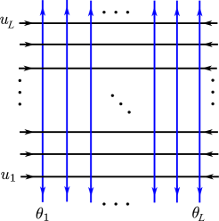
Figure 3.5: The domain wall partition function of six vertex model. Notice that the configurations at the four boundaries are fixed.

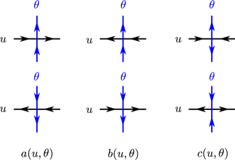
Figure 3.6: The six different vertex configuration, with their weights defined in equation (3.74).

The sum in the DWPF concernes all the configurations involving the six types of vertices shown in figure 3.6, the weight of each type of vertex being given by

$$a(u,\theta)=u-\theta+i/2\,,\qquad b(u,\theta)=u-\theta-i/2\,,\qquad c(u,\theta)=i\,.$$ (3.74)

The DWPF can be alternatively defined in the language of the algebraic Bethe Ansatz as

$$Z_{L}({{\bf u}}|{\text{\boldmath$\theta$}})\equiv\langle\,\downarrow^{L}\!|\prod_{k=1}^{L}B(u_{k};{\text{\boldmath$\theta$}})|\!\uparrow^{L}\,\rangle\,,$$ (3.75)

where ${\text{\boldmath$\theta$}}=\{\theta_{1},\cdots,\theta_{L}\}$ is the set of inhomogeneities and ${{\bf u}}=\{u_{1},\cdots,u_{L}\}$ are the magnon rapidities. The mapping from the six vertex configuration to the algebraic Bethe Ansatz language, explained at length in OmarFreezing , is based on the interpretation of the six non-trivial vertex configurations (3.74) as the non-zero elements of the Lax matrix $\mathrm{L}(u)$. The black, horizontal lines correspond to copies of the auxiliary space, while the blue vertical lines correspond to the quantum space. Conventionally, the Lax matrix acts from NE to SW. The DWBC configuration with all the arrows pointing upwards on the upper edge corresponds to the vacuum $|\!\uparrow^{L}\,\rangle$, the horizontal lines with incoming arrows correspond to operators $B(u)$ and the horizontal lines with outgoing arrows correspond to operators $C(u)$. The symmetry properties of the Lax matrix are inherited by the six-vertex configuration,

$$\mathrm{L}_{n}(u)=\mathrm{L}_{n}(u)^{t,t_{0}}=\sigma_{n}^{2}\sigma^{2}\,\mathrm{L}_{n}(u)\,(\sigma_{n}^{2}\sigma^{2})^{-1}\;,$$ (3.76)

where $t,t_{0}$ mean transposition in the quantum and in the auxiliary spaces respectively. The simultaneous transposition in the two spaces, followed by the conjugation with $\sigma^{2}$ in the two spaces, amounts to the rotation of the corresponding vertex by $180^{\circ}$. The conjugation is necessary to keep the orientation of the arrows unchanged.

When applied to the untwisted monodromy matrix, the simultaneous transposition reverses the order of the sites on the chain, as one can see as well from the graphical interpretation,

$$\mathrm{T}(u)^{t,t_{0}}=\mathrm{L}_{L}(u)^{t,t_{0}}\ldots\mathrm{L}_{1}(u)^{t,t_{0}}=\mathrm{L}_{L}(u)\ldots\mathrm{L}_{1}(u)\equiv\bar{\mathrm{T}}(u)\;.$$ (3.77)

In components, this means for example that $B^{t}(u)=\bar{C}(u)$, where the bar denotes the reversal of the order of the sites in the chain. Taking the transpose in the quantum space and using the fact that the DWPF is symmetric in the variables $\theta_{1},\ldots,\theta_{L}$, so that the order of the sites is irrelevant, one gets

$$Z_{L}({{\bf u}}|{\text{\boldmath$\theta$}})=\langle\,\uparrow^{L}\!|\prod_{k=1}^{L}B^{t}(u_{k};{\text{\boldmath$\theta$}})|\!\downarrow^{L}\,\rangle=\langle\,\uparrow^{L}\!|\prod_{k=1}^{L}C(u_{k};{\text{\boldmath$\theta$}})|\!\downarrow^{L}\,\rangle\,.$$ (3.78)

The second equality in (3.76) translates into the following equality for the monodromy matrix

$$\mathrm{T}(u)=\Sigma_{2}\sigma^{2}\;\mathrm{T}(u)\;(\Sigma_{2}\sigma^{2})^{-1}\;,$$ (3.79)

with $\Sigma_{2}$ defined in (3.63). Written in components, this gives the relation (3.62) between the $B(u)$ and $C(u)$ operators. Given that the action of $\Sigma_{2}$ on the vacua is $\Sigma_{2}\,|\!\uparrow^{L}\,\rangle=(-1)^{L}\,|\!\downarrow^{L}\,\rangle$ and $\Sigma_{2}\,|\!\downarrow^{L}\,\rangle=|\!\uparrow^{L}\,\rangle$ the DWPF can take the alternative form

$$Z_{L}(\mathbf{u}|{\text{\boldmath$\theta$}})=\langle\,\uparrow^{L}\!|\prod_{k=1}^{L}C(u_{k};{\text{\boldmath$\theta$}})|\!\downarrow^{L}\,\rangle\,.$$ (3.80)

The equality of (3.75), (3.78) and (3.80) expresses the invariance of the DWPF under reversal of the arrows. If one views the action of the monodromy matrix as an evolution in a (discrete) time, the rotation with $180^{\circ}$ clockwise can be viewed as a PT transformation, and the transformations properties above as a CPT invariance. It is instructive to go back and interpret equation (3.1) in terms of six-vertex configuration. The second line can be written in terms of a rectangular six-vertex configuration. Now we insert the resolution of identity between the two rotations and apply transposition and conjugation with $\Sigma_{2}$ in the first block,

$$(-1)^{L-M_{2}} \langle\,\downarrow^{L}\!|\prod_{j=1}^{M_{2}}B(u_{2,j})\,\mathrm{g}_{2}^{-1}\mathrm{g}_{1}\,\prod_{k=1}^{M_{1}}B(u_{1,k})|\!\uparrow^{L}\,\rangle\,=$$ (3.81)

$$=\!\!\!\!\sum_{\varepsilon_{1},\ldots,\varepsilon_{L}=\uparrow,\downarrow} \!\!\!\!\langle\varepsilon_{1},\ldots,\varepsilon_{L}|\,\Sigma_{2}\,\mathrm{g}_{2}\,\prod_{j=1}^{M_{2}}\bar{B}(u_{2,j})|\!\uparrow^{L}\,\rangle\,\langle\varepsilon_{1},\ldots,\varepsilon_{L}|\,\mathrm{g}_{1}\,\prod_{k=1}^{M_{1}}B(u_{1,k})|\!\uparrow^{L}\,\rangle\,.$$

In the six-vertex model picture, the first line corresponds to the ordinary domain wall partition (with the global rotations inserted in the middle) whereas the second line corresponds to the configuration where the lower half is rotated by 180^∘ (see figure 3.7). The action of the operator $\Sigma_{2}$ is symbolized by the blobs in the middle of the lines. The effect of such blob is a multiplication by a factor $(-1)$ if $\varepsilon=\uparrow$.

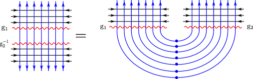
Figure 3.7: Relation between six vertex model configuration and the spin vertex formalism. The blobs symbolize the action of the operator $\Sigma_{2}$: an extra factor $(-1)$ if $\varepsilon=\uparrow$.

Less obvious are the transformation properties under rotation of the six-vertex configuration with $90^{\circ}$. By the space-time analogy above we can consider this transformation as an exchange of space and time, which in the context of integrable field theories goes under the name of mirror transformation. We are using this term here, although there might be differences with other instances of mirror transformations. Under the mirror transformation we get another domain wall boundary condition configuration with the inhomogeneities and rapidities exchanged as in figure 3.6. The vertices in figure 3.6 transform as follows

$$a(u,\theta) \to b(\theta,u)=-a(u,\theta)\;,$$ (3.82)

$$b(u,\theta) \to a(\theta,u)=-b(u,\theta)\,,$$

$$c(u,\theta) \to c(\theta,u)=c(u,\theta)\,.$$

We conclude that the rotated DWPF shown in figure 3.8 is equal to the non-rotated one up to a sign. To compute this sign we need to know the parity of number of vertices of type $a$ and $b$, $N_{a}$ and $N_{b}$. Due to the particular type of boundary condition we consider, on each line there should be one type $c$ vertex. For the DWPF the sign is then given by

$$(-1)^{N_{a}+N_{b}}=(-1)^{L(L-1)}=1$$ (3.83)

so that

$$Z_{L}({\text{\boldmath$\theta$}}|\mathbf{u})=Z_{L}({\mathbf{u}}|{\text{\boldmath$\theta$}})\;.$$ (3.84)

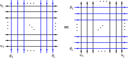
Figure 3.8: We rotate the configuration in figure  3.6 by 90^∘ clockwise, the expression for the partition function is invariant. The interpretations of the two diagrams are different. The roles of rapidities and inhomogeneities are exchanged in the two configurations.

Therefore, the DWPF in the mirror representation is given by

$$Z_{L}({\text{\boldmath$\theta$}}|\mathbf{u})=\langle\,\uparrow^{L}\!|\prod_{k=1}^{L}C(\theta_{k};\mathbf{u})|\!\downarrow^{L}\,\rangle=\langle\,\downarrow^{L}\!|\prod_{k=1}^{L}B(\theta_{k};\mathbf{u})|\!\uparrow^{L}\,\rangle.$$ (3.85)

3.3 Global rotation and twist

The next step is to find the mirror representation of the partition functions in the six vertex model in presence of a global rotation. We suppose that, as in equation (3.73) the rotation acts directly on the vacuum. The partition function we study is depicted in figure  (3.9). On the l.h.s. the partition function corresponds to

$$\texttt{lhs}=\,\langle\uparrow^{L}\!|\,\mathrm{g}^{t}\,C(u_{1}) \cdots C(u_{M})|\!\downarrow^{L}\rangle=(-1)^{L-M}\langle\downarrow^{L}\!|\,\mathrm{g}^{-1}\,B(u_{1})\cdots B(u_{M})|\!\uparrow^{L}\rangle$$

$$=\langle\downarrow^{L}\!|B(u_{1})\cdots B(u_{M})\,\mathrm{g}\,|\!\uparrow^{L}\rangle\,,$$ (3.86)

where in the last two equalities we have used the conjugation with the matrix $\Sigma_{2}$ and transposition in the quantum space respectively, as discussed in the previous subsection, and $\mathrm{g}^{-1}=\Sigma_{2}\,\mathrm{g}^{t}\,\Sigma_{2}^{-1}$. After rotation with $90^{\circ}$ the partition function acquires a sign $(-1)^{N_{a}+N_{b}}=(-1)^{M(L-1)}$, cf. equation (3.82), and the rotation in the quantum space $\mathrm{g}$ is replaced by the twist matrix $\mathrm{K}^{t}$ acting in the auxiliary space

$$\texttt{rhs}=(-1)^{M(L-1)}\langle\downarrow^{M}|B_{\mathrm{K}^{t}|0}(\theta_{1})\cdots B_{\mathrm{K}^{t}|0}(\theta_{L})|\uparrow^{M}\rangle$$ (3.87)

We conclude that after the mirror transformation the rotation in the quantum space $\mathrm{g}$ is replaced with the twist $\mathrm{K}^{t}$. In particular

$$\mathrm{g}=e^{zS^{-}}\qquad\buildrel{\rm mirror}\over{\longleftrightarrow}\qquad\mathrm{K}^{t}=e^{z\sigma^{+}}\;.$$ (3.88)

Since in the mirror representation the $B$-operators are twisted, we can apply the SoV formalism.

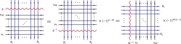
Figure 3.9: The mirror representation in the presence of global rotation. After turning the diagram 90^∘, the global rotation plays the role of a twist.

3.4 Two dual integral representations for the scalar product

Both the expressions (3.3) and (3.87) can be written as multiple integrals using SoV method. For (3.3) the integral representation was derived in KKN , after introducing an extra twist which can be subsequently set to zero. Since we are going to compute scalar products for sub-chains, the rapidities are not assumed to be on shell. Nevertheless one can apply the argument of KKN to carry on the computation.

Consider first the lhs, eq. (3.3), which we denote using the same notation as above (but with $|{\text{\boldmath$\theta$}}|\geq|{{\bf u}}|$). In order to go to the SoV representation, we introduce a left twist $\mathrm{K}_{\epsilon|0}$ and then take the limit $\epsilon\to 0$. For simplicity we take $\mathrm{g}=e^{zS^{-}}$. Only one term in the expansion of the exponent survives and the result is

$$\texttt{lhs}\,\to\langle\,\downarrow^{L}\!|B_{\epsilon}(u_{1})\ldots B_{\epsilon}(u_{M})\,e^{zS^{-}}|\!\uparrow^{L}\,\rangle,$$ (3.89)

In this way we represent this expectation value as a multiple integral in the separated variables. The derivation is the one from KKN , after noticing that only one term in the expansion of the exponent survives (the one which compensates the extra $S_{z}$ charge $L-M$). We give only the final result,

lhs $$=i^{L}{z^{L-M}\over(L-M)!}\ \;\Xi_{{\text{\boldmath$\theta$}}}\oint\limits_{{\mathcal{C}}_{\text{\boldmath$\theta$}}}\prod_{j=1}^{L}{dx_{j}\over 2\pi i}\ {Q_{{\bf u}}(x_{j})\ e^{2\pi(j-1)x_{k}}\over Q_{\text{\boldmath$\theta$}}^{+}(x_{j})Q_{\text{\boldmath$\theta$}}^{-}(x_{j})}\ \prod_{j<k}^{L}(x_{j}-x_{k})\ \left(\sum_{j=1}^{L}x_{j}\right)^{L-M}$$ (3.90)

where the function $\Xi_{{\text{\boldmath$\theta$}}}$ is defined by

$$\Xi_{{\text{\boldmath$\theta$}}}= \,\frac{\prod_{j<k}(\theta_{j}-\theta_{k})(\theta_{j}-\theta_{k}+i)(\theta_{j}-\theta_{k}-i)}{\prod_{j<k}\left(e^{2\pi\theta_{j}}-e^{2\pi\theta_{k}}\right)}$$ (3.91)

and the contour ${\mathcal{C}}_{\text{\boldmath$\theta$}}$ encircles the sets ${\text{\boldmath$\theta$}}^{+}$ and ${\text{\boldmath$\theta$}}^{-}$. Now we write integral representation for the rhs, eqn. (3.87),

$$\begin{aligned} \texttt{rhs}\,&=(-1)^{M(L-1)}\,i^{M}\ z^{L-M}\ \Xi_{\mathbf{u}}\ \oint\limits_{{\mathcal{C}}_{{\bf u}}}\prod_{j=1}^{M}{dx_{j}\over 2\pi i}\ \ \prod_{j<k}^{M}(x_{j}-x_{k})\ \prod_{k=1}^{M}{Q_{\text{\boldmath$\theta$}}(x_{k})\ e^{2\pi(k-1)x_{k}}\over Q_{{\bf u}}^{+}(x_{k})\ Q_{{\bf u}}^{-}(x_{k})},\ \ \ \end{aligned}$$ (3.92)

where $\Xi_{\mathbf{u}}$ is defined similarly as in (LABEL:eq:Xi) and the contour ${\mathcal{C}}_{{\bf u}}$ encircles the all points ${\mathbf{u}^{+}}$ and ${\mathbf{u}^{-}}$.

4 Three-point functions in the SoV representation

In this section, we compute the structure constant using the spin vertex formalism in JKPS ; KKNv ; StringBit . After the mirror transformation, we can compute both the spin vertex and the wave functions of the external states in the SoV representation, and combining them we get the final result. We can of course do the computation with the generic twists, but in fact it is enough to consider the triangular twists of the following form

$$\mathrm{K}_{z_{a}}=e^{z_{a}\,\sigma^{+}}=\left(\begin{array}[]{cc}1&\ z_{a}\\ 0&\ 1\\ \end{array}\right),\qquad a=1,2,3.$$ (4.95)

The reason is that the twists in the mirror representation come from the global rotations in the original representation. As is shown in (3.68), if we start with on-shell Bethe states which satisfy highest weight conditions, the most general global rotation can be reduced to the rotation of the form $\mathrm{g}_{z}=e^{z\,S^{-}}$, together with some factors which are not relevant. So we can define our external states as $|\psi\rangle=e^{zS^{-}}|\mathbf{u}\rangle$ without loss of generality. The global rotation $e^{zS^{-}}$, upon performing the mirror transformation, turns into the twist of the form (4.95).

4.1 Spin vertex and the mirror transformation

We are interested in computing the three-point function for three operators belonging to the so-called left $\mathfrak{su}(2)_{L}$ subsector of the $\mathfrak{so}(4)\simeq\mathfrak{su}(2)_{{}_{\mathrm{L}}}\otimes\mathfrak{su}(2)_{{}_{\mathrm{R}}}$ sector of the ${\cal N}=4$ SYM theory. This sector is made by the scalar fields $X,\ \bar{X},\ Z,\ \bar{Z}$ which belong to the bi-fundamental representation of $\mathfrak{su}(2)_{\mathrm{L}}\otimes\mathfrak{su}(2)_{{}_{\mathrm{R}}}$,

$$|Z\rangle=|\!\uparrow\rangle_{{}_{\mathrm{L}}}\otimes|\!\uparrow\rangle_{{}_{\mathrm{R}}}\equiv|\!\uparrow\uparrow\rangle\;,\qquad|\bar{Z}\rangle=|\!\downarrow\rangle_{{}_{\mathrm{L}}}\otimes|\!\downarrow\rangle_{{}_{\mathrm{R}}}\equiv|\!\downarrow\downarrow\rangle\;,$$ (4.96)

$$|X\rangle=|\!\uparrow\rangle_{{}_{\mathrm{L}}}\otimes|\!\downarrow\rangle_{{}_{\mathrm{R}}}\equiv|\!\uparrow\downarrow\rangle\;,\qquad|\bar{X}\rangle=-|\!\downarrow\rangle_{{}_{\mathrm{L}}}\otimes|\!\uparrow\rangle_{{}_{\mathrm{R}}}\equiv-|\!\downarrow\uparrow\rangle\;.$$

Again, we are using the vertex formalism from KKNv ; JKPS ; StringBit to compute the overlap of the three spin chains. At tree level, the three vertex $\langle\mathrm{V}_{3}|$ is composed by the three singlets ${}_{(ij)}\langle\mathrm{V}_{2}|$ corresponding to the bridges connecting the piece $(ij)$ of the chain $i$ with the piece $(ji)$ of the chain $j$,

$$\langle\mathrm{V}_{3}|=\,_{(12)}\langle\mathrm{V}_{2}|\otimes\,_{(23)}\langle\mathrm{V}_{2}|\otimes\,_{(31)}\langle\mathrm{V}_{2}|\,.$$ (4.97)

We consider the case where the non-trivial magnon excitations belong only to the left sector. The three external Bethe states with global rotations $\mathrm{g}_{z_{a}}\otimes\mathrm{g}_{\hat{z}_{a}}$ ($a=1,2,3$) are given by

$$|\Psi_{a}\rangle =|\psi_{a}\rangle_{{}_{\mathrm{L}}}\otimes|\hat{\psi}_{a}\rangle_{{}_{R}}$$ (4.98)

with the right components being rotated pseudovacua,

$$|\psi_{a}\rangle_{{}_{\mathrm{L}}}=\mathrm{g}_{z_{a}}|\mathbf{u}_{a}\rangle_{{}_{\mathrm{L}}},\quad|\hat{\psi}_{a}\rangle_{{}_{\mathrm{L}}}=\hat{\mathrm{g}}_{\hat{z}_{a}}|\uparrow^{L_{a}}\rangle_{{}_{\mathrm{R}}}\qquad(a=1,2,3).$$ (4.99)

The spin vertex also splits into two identical parts $\langle\mathrm{V}_{3}|={{}_{{}_{\text{L}}}\langle}\mathrm{V}_{3}|\otimes{{}_{{}_{\text{R}}}\langle}\mathrm{V}_{3}|$. This insures the complete factorization of the left and right sectors,

$$\langle\mathrm{V}_{3}|\ |\Psi_{1}\rangle\,|\Psi_{2}\rangle\,|\Psi_{3}\rangle=\left(\langle\mathrm{V}_{3}|\ |\psi_{1}\rangle\,|\psi_{2}\rangle\,|\psi_{3}\rangle\right)_{{}_{\mathrm{L}}}\;\left(\langle\mathrm{V}_{3}|\,\hat{\mathrm{g}}_{\hat{z}_{1}}\,|\uparrow^{L_{1}}\rangle\,\hat{\mathrm{g}}_{\hat{z}_{2}}\,|\uparrow^{L_{2}}\rangle\,\hat{\mathrm{g}}_{\hat{z}_{3}}|\uparrow^{L_{3}}\rangle\right)_{{}_{\mathrm{R}}}.$$ (4.100)

The right piece is easily calculted and is equal to $(\hat{z}_{12})^{L_{12}}(\hat{z}_{23})^{L_{23}}(\hat{z}_{31})^{L_{31}}$, where $L_{ab}=\frac{1}{2}(L_{a}+L_{b}-L_{c})$, $(a,b,c=1,2,3)$.

As mentioned before, we take the following external states

$$|\psi_{a}\rangle= \,e^{z_{a}S^{-}_{a}}|\mathbf{u}_{a}\rangle=\prod_{j=1}^{M_{a}}B(u_{a,j})\ e^{z_{a}S^{-}_{a}}\,|\uparrow^{L_{a}}\rangle,\qquad a=1,2,3.$$ (4.101)

We are going to concentrate from now on on the structure constant in the left sector and drop the L index on the states and on the vertex

$$C_{123}^{\mathrm{L}}=\langle\mathrm{V}_{3}|\,|\psi_{1}\rangle_{{}_{\text{L}}}|\psi_{2}\rangle_{{}_{\text{L}}}|\psi_{3}\rangle_{{}_{\text{L}}}.$$ (4.102)

The structure constant above has a representation in terms of 6-vertex model partition function on the diagram of figure 4.10. Apart from the blobs, this diagram is nothing but a redrawing of the hexagon DWPF in figure 1.1 (in the hexagon DWPF there was no need to put blobs along the “bridges”).

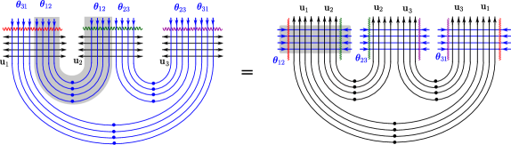
Figure 4.10: The three-point function before and after the mirror transformation. One can see that the role of impurities and rapidities are exchanged, as in the case of scalar products. In addition, the global rotation becomes twist in the mirror representation, as in the scalar product.

We will perform a mirror transformation on the six-vertex configuration of the three-point function as is shown in figure 4.10. We rotate the left subchains clockwise and the right subchains anti-clockwise and combine together the neighboring subchains, as is shown in the shaded region of figure 4.10. Potentially, there is some minus sign coming from the transition from the direct vertex $\langle\mathrm{V}_{3}|$ to the mirror vertex $\langle\tilde{\mathrm{V}}_{3}|$. But since the signs coming from “bridges” in the direct and the mirror vertex are related, since ones constitute boundary conditions for the others, we neglect any overall sign which may occur. From the 6-vertex configuration, we see that we need to compute the following mirror structure constant

$${C}_{123}^{\mathrm{L}}=\tilde{C}_{123}^{\mathrm{L}}\equiv\langle\tilde{\mathrm{V}}_{3}||\tilde{\psi}^{(12)}\rangle|\tilde{\psi}^{(23)}\rangle\,|\tilde{\psi}^{(31)}\rangle.$$ (4.103)

In what follows, we put a tilde on the operators which are in the mirror representation. The three mirror external states are now

$$|{\tilde{\psi}^{(ab)}}\rangle= \,\prod_{k=1}^{L_{ab}}\tilde{B}_{z_{a}|-z_{b}}(\theta^{(ab)}_{k})\,|\!\!\uparrow^{M_{a}+M_{b}}\rangle,\qquad(ab)=(12),(23),(31)\,,$$ (4.104)

where the operators $\tilde{B}_{z_{a}|-z_{b}}(\theta)$ are the matrix elements (first row and the second column) of the following double twisted monodromy matrices

$$\tilde{\mathrm{T}}_{z_{a}|-z_{b}}(\theta)= \,\mathrm{K}_{z_{a}}\,\prod_{j=1}^{M_{a}}\mathrm{L}_{n}(\theta-u_{a,j})\prod_{k=1}^{M_{b}}\mathrm{L}_{k}(\theta-u_{b,k})\,\mathrm{K}_{-z_{b}}.$$ (4.105)

We can construct the SoV states for the three double twisted spin chains, which are denoted as $|{{{\bf x}}}\rangle_{z_{a}|-z_{b}}$.

4.2 Spin vertex in SoV representation

In order to compute the spin vertex, we apply the important property (3.71). In the presence of the twists, this property is modified to be

$$\,\langle{\mathrm{V}}_{2}|A^{(1)}_{z_{1}|-z_{2}}(u)=\langle{\mathrm{V}}_{2}|D^{(2)}_{z_{2}|-z_{1}}(u),\quad\langle{\mathrm{V}}_{2}|B^{(1)}_{z_{1}|-z_{2}}(u)=-\langle{\mathrm{V}}_{2}|B^{(2)}_{z_{2}|-z_{1}}(u),$$ (4.106)

$$\,\langle{\mathrm{V}}_{2}|D^{(1)}_{z_{1}|-z_{2}}(u)=\langle{\mathrm{V}}_{2}|A^{(2)}_{z_{2}|-z_{1}}(u),\quad\langle{\mathrm{V}}_{2}|C^{(1)}_{z_{1}|-z_{2}}(u)=-\langle{\mathrm{V}}_{2}|C^{(2)}_{z_{2}|-z_{1}}(u).$$

By putting one of the twists to zero, we obtain similar relations for the left or right twisted monodromy matrices. Notice that the left twisted monodromy matrix is translated to a right twisted one by the spin vertex and vice versa. Using these relations, one can show that

$$\langle\mathrm{V}_{2}|\,|{{\bf x}}\rangle_{z|0}|{{\bf y}}\rangle_{0|-z}={{}_{z|0}\langle}{{\bf y}}|{{\bf x}}\rangle_{z|0}=(\mu_{z|0}({{\bf x}}))^{-1}\delta_{{{\bf x}},{{\bf y}}}$$ (4.107)

where $\delta_{{{\bf x}},{{\bf y}}}=\delta_{x_{1},y_{1}}\cdots\delta_{x_{N},y_{N}}$ and $\mu_{z|0}({{\bf x}})$ is the Sklyanin measure.

We can write the three-point spin vertex in the SoV using the resolution of identities of the SoV basis. Denoting by ${{\bf x}}^{(ab)}$ are the SoV variables associated with the state $\tilde{\psi}^{(ab)}$, we write the 3-vertex as a triple sum

$$\langle\tilde{\mathrm{V}}_{3}|=\,\sum_{{{\bf x}}^{(12)},{{\bf x}}^{(23)},{{\bf x}}^{(31)}}\tilde{\mathrm{V}}({{\bf x}}^{(12)},{{\bf x}}^{(23)},{{\bf x}}^{(31)}) \,\mu_{z_{1}|-z_{2}}({{\bf x}}^{(12)})\,\mu_{z_{2}|-z_{3}}({{\bf x}}^{(23)})\,\mu_{z_{3}|-z_{1}}({{\bf x}}^{(31)})$$ (4.108)

$$\,\times{{}_{z_{1}|-z_{2}}\langle{{\bf x}}^{(12)}|}\otimes{{}_{z_{2}|-z_{3}}\langle{{\bf x}}^{(23)}|}\otimes{{}_{z_{3}|-z_{1}}\langle{{\bf x}}^{(31)}|},$$

where the coefficient function $\tilde{\mathrm{V}}({{\bf x}}^{(ab)})$ is given by

$$\tilde{\mathrm{V}}({{\bf x}}^{(12)},{{\bf x}}^{(23)},{{\bf x}}^{(31)})=\langle\tilde{\mathrm{V}}_{3}|\,|{{\bf x}}^{(12)}\rangle_{z_{1}|-z_{2}}\otimes|{{\bf x}}^{(23)}\rangle_{z_{2}|-z_{3}}\otimes|{{\bf x}}^{(31)}\rangle_{z_{3}|-z_{1}}.$$ (4.109)

In order to compute this function, we first split the SoV states as is described in section 2.3 appendix C,

$$|{{\bf x}}^{(12)}\rangle_{z_{1}|-z_{2}}=\sum_{{{\bf y}}_{1},\,{{\bf y}}_{2}}\mu_{z_{1}|0}({{\bf y}}_{1})\ \mu_{0|-z_{2}}({{\bf y}}_{2})\ \Phi({{\bf y}}_{1};{{\bf y}}_{2}|{{\bf x}}^{(12)})\ \,|{{\bf y}}_{1}\rangle_{z_{1}|0}\otimes|{{\bf y}}_{2}\rangle_{0|-z_{2}},$$ (4.110)

and similarly for $|{{\bf x}}^{(23)}\rangle_{z_{2}|-z_{3}}$ and $|{{\bf x}}^{(31)}\rangle_{z_{3}|-z_{1}}$. Acting the states on the three-point spin vertex and using (4.107), we obtain

$$\tilde{\mathrm{V}}({{\bf x}}^{(12)},{{\bf x}}^{(23)},{{\bf x}}^{(31)})= \,\sum_{{{\bf y}}_{1},{{\bf y}}_{2},{{\bf y}}_{3}}\mu_{z_{1}|0}({{\bf y}}_{1})\ \mu_{z_{2}|0}({{\bf y}}_{2})\ \mu_{z_{3}|0}({{\bf y}}_{3})$$ (4.111)

$$\,\times\Phi({{\bf y}}_{1};{{\bf y}}_{2}|{{\bf x}}^{(12)})\ \Phi({{\bf y}}_{2};{{\bf y}}_{3}|{{\bf x}}^{(23)})\ \Phi({{\bf y}}_{3};{{\bf y}}_{1}|{{\bf x}}^{(31)}).$$

The eigenvalues for the three sets of separated variables of the subchains are

$${{\bf y}}_{1}=\mathbf{u}_{1}\pm{\textstyle{i\over 2}},\quad{{\bf y}}_{2}=\mathbf{u}_{2}\pm{\textstyle{i\over 2}},\quad{{\bf y}}_{3}=\mathbf{u}_{3}\pm{\textstyle{i\over 2}}\,,$$ (4.112)

where ${{\bf y}}_{a}=\mathbf{u}_{a}\pm{\textstyle{i\over 2}}$ is understood as $y_{a,k}=u_{a,k}\pm{\textstyle{i\over 2}}$, ($k=1,\cdots,M_{a}$).

4.3 The wave functions

The external states in the mirror representation are given in (4.104). Acting these states on the spin vertex (4.108) and using the property of the SoV basis

$${}_{z_{1}|-z_{2}}\langle{{\bf x}}|\tilde{B}_{z_{1}|-z_{2}}(\theta)=(z_{1}-z_{2})\,Q_{{{\bf x}}}(\theta)\,{{}_{z_{1}|-z_{2}}\langle{{\bf x}}|},$$ (4.113)

we obtain the wave functions of the mirror Bethe states

$$_{z_{a}|-z_{b}}\langle{{\bf x}}^{(ab)}|\tilde{\psi}^{(ab)}\rangle= \,(-1)^{L_{a,b}(M_{a}+M_{b})}\,(z_{a}-z_{b})^{L_{ab}}\,f_{z_{a}|-z_{b}}({{\bf x}}^{(ab)})\prod_{k=1}^{M_{a}+M_{b}}Q_{{\text{\boldmath$\theta$}}^{(ab)}}(x_{k}^{(ab)})\,,$$ (4.114)

where the phase factor $(-1)^{L_{ab}(M_{a}+M_{b})}$ comes from the rewriting of products of $Q$-functions

$$\prod_{j=1}^{L_{ab}}Q_{{{\bf x}}_{a}}(\theta^{(ab)}_{j})\equiv({\text{\boldmath$\theta$}}^{(ab)}-{{\bf x}}^{(ab)})=(-1)^{L_{ab}(M_{a}+M_{b})}\prod_{k=1}^{M_{a}+M_{b}}Q_{{\text{\boldmath$\theta$}}^{(ab)}}(x^{(ab)}).$$ (4.115)

The functions $f_{z_{a}|-z_{b}}({{\bf x}})$ are the projection of SoV basis on the pseudovacuum and are given by

$$f_{z_{a}|-z_{b}}({{\bf x}}^{(ab)})= \,{{}_{z_{a}|-z_{b}}\langle{{\bf x}}^{(ab)}|}\!\!\uparrow^{M_{a}+M_{b}}\rangle.$$ (4.116)

From (2.53) the projection of SoV basis on the pseudovacuum for the triangular twists of the form (4.95) is simply

$${{}_{z_{a}|-z_{b}}\langle}{{\bf x}}|\!\uparrow^{L}\,\rangle=1.$$ (4.117)

4.4 The final result

We can now assemble the results from the previous subsections and write down the final result for the structure constant. Plugging (4.108), (4.109), (4.111) and (4.114) into (4.103), we obtain

$$C_{123}^{\mathrm{L}}= \prod_{a=1}^{3}(-1)^{L_{a}M_{a}}\prod_{(ab)}z_{ab}^{L_{ab}}\ \sum_{\{{{\bf x}}^{(ab)}\}}\sum_{\{{{\bf y}}_{a}\}}$$

$$\times \ \prod_{a=1}^{3}\mu_{z_{a}|0}({{\bf y}}_{a})\ \prod_{(ab)}\mu_{z_{a}|-z_{b}}({{\bf x}}^{(ab)})\ \ \Phi({{\bf y}}_{a};{{\bf y}}_{b}|{{\bf x}}^{(ab)})\ \ \prod_{k=1}^{M_{a}+M_{b}}Q_{{\text{\boldmath$\theta$}}^{(ab)}}(x^{(ab)}_{k}),$$ (4.118)

where we have defined $z_{ab}=z_{a}-z_{b}$. In (4.4), the summation is over all the possible eigenvalues of all the SoV variables. The structure of the summand is the product of Sklyanin measures of the three spin chains and three subchains, the three splitting functions which originate from cutting the spin chains, and the three wave functions.

Similar to the scalar product, there’s another way of writing $C_{123}^{\mathrm{L}}$ which converts the sum over eigenvalues of separated variables to a multiple contour integral. The derivation of the integral representation is analogues to the scalar product in KKN . The result is given by the integral

$$C_{123}^{\mathrm{L}}=\,\texttt{factor}\times\oint\limits_{\{{{\bf u}}_{1,2,3}\pm i/2\}}\prod_{(ab)} \frac{\Gamma\left(i(\mathbf{u}_{a}^{+}-\mathbf{u}_{b}^{-})\right)}{\Gamma\left(i({{\bf y}}_{a}-{{\bf y}}_{b})\right)}\ \frac{\Gamma\left(1-i(\mathbf{u}_{a}^{+}-{{\bf x}}^{(ab)})\right)\Gamma\left(1+i(\mathbf{u}_{b}^{-}-{{\bf x}}^{(ab)})\right)}{\Gamma\left(1-i({{\bf y}}_{a}-{{\bf x}}^{(ab)})\right)\Gamma\left(1+i({{\bf y}}_{b}-{{\bf x}}^{(ab)})\right)}$$

$$\times({{\bf x}}^{(ab)}-{\text{\boldmath$\theta$}}^{(ab)})\ T(z_{1},z_{2},z_{3})\ d\mu({{\bf x}}^{(ab)})\ d\mu({{\bf y}}_{a}),$$ (4.119)

where $(ab)=(12),(23),(31)$. We denoted by $T(z_{1},z_{2},z_{3})$ the factor in the integrand which depends on the twists:

$$T(z_{1},z_{2},z_{3}) =\prod_{(ab)}\left({iz_{ab}\over z_{a}}\right)^{N_{+}^{{{\bf y}}_{b}}}\left({z_{ab}\over iz_{b}}\right)^{N_{-}^{{{\bf y}}_{a}}}(-z_{a})^{N_{+}^{{{\bf x}}^{(ab)}}}(z_{b})^{N_{-}^{{{\bf x}}^{(ab)}}}$$ (4.120)

with

$$N^{{{\bf y}}_{a}}_{\pm}\equiv{M_{a}\over 2}\mp i\sum_{j=1}^{M_{a}}(y_{a,j}-u_{a,j}),\ \ N^{{\bf x}}_{\pm}={M_{a}+M_{b}\over 2}\mp i\!\!\!\sum_{j=1}^{M_{a}+M_{b}}(x^{(ab)}_{j}-u_{a,j}-u_{b,j}).\ \$$ (4.121)

The measures $d\mu({{\bf x}}^{(ab)})$ and $\mu({{\bf y}}_{a})$ for the spin chains and subchains are defined by

$$d\mu({{\bf x}}^{(ab)})= \,\prod_{k=1}^{M_{a}+M_{b}}\frac{dx^{(ab)}_{k}}{2\pi i}\frac{\Delta({{\bf x}}^{(ab)})\Delta(e^{2\pi{{\bf x}}^{(ab)}})}{({{\bf x}}^{(ab)}-{{\bf u}}_{a}^{+})({{\bf x}}^{(ab)}-{{\bf u}}_{a}^{-})({{\bf x}}^{(ab)}-{{\bf u}}^{+}_{b})({{\bf x}}^{(ab)}-{{\bf u}}^{-}_{b})},$$ (4.122)

$$d\mu({{\bf y}}_{a})= \,\prod_{j=1}^{M_{a}}\frac{dy_{a,j}}{2\pi i}\,\frac{\Delta({{\bf y}}_{a})\Delta(e^{2\pi{{\bf y}}_{a}})}{({{\bf y}}^{a}-{{\bf u}}^{+}_{a})({{\bf y}}_{a}-{{\bf u}}^{-}_{a})}.$$ (4.123)

Finally, the overall factor reads, up to a phase factor,

$$\texttt{factor}= \,\frac{1}{(M_{1}+M_{2})!(M_{2}+M_{3})!(M_{3}+M_{1})!\,M_{1}!M_{2}!M_{3}!}$$ (4.124)

$$\,\times\prod_{(ab)}(z_{ab})^{L_{ab}-M_{a}-M_{b}}\prod_{a}(z_{a})^{-M_{a}}$$

$$\,\times\Xi_{\mathbf{u}_{1}\cup\mathbf{u}_{2}}\times\Xi_{\mathbf{u}_{2}\cup\mathbf{u}_{3}}\times\Xi_{\mathbf{u}_{3}\cup\mathbf{u}_{1}}\times\Xi_{\mathbf{u}_{1}}\times\Xi_{\mathbf{u}_{2}}\times\Xi_{\mathbf{u}_{3}}.$$

The factor comes from the product of the common factor in (4.4) and the part of Sklyanin measures which do not depend on SoV variables, Eq. (LABEL:eq:Xi).

As proved in KKNv , the $z_{a}$ dependence is completely determined as follows by the Ward identity when operators are primary:

$$C_{123}^{L}\ \propto\ (z_{12})^{L_{12}-M_{1}-M_{2}+M_{3}}\ (z_{23})^{L_{23}-M_{2}-M_{3}+M_{1}}\ (z_{31})^{L_{31}-M_{3}-M_{1}+M_{2}}\,.$$ (4.125)

One way to see this $z$-factorisation explicitly is to first compute the integral, use the Bethe equations and eliminate $z$’s. Although we haven’t succeeded, it would be much more desirable if we could rewrite the integrand (using Bethe equations or Baxter equations) in such a way that the $z$-independence becomes manifest. We leave this as an important future problem.

5 Conclusion and prospects

In this paper, we derived a new integral expression for three-point functions in the $\mathfrak{su}(2)$ sector of $\mathcal{N}=4$ SYM using Sklyanin’s separation of variables. In order to apply the SoV method, we first mapped the three-point function to the partition function of the six-vertex model with a hexagonal boundary and then performed 90^∘ rotations, which we call mirror rotations. The SoV approach can be readily used after this manipulation without the need of introducing boundary twists. The intriguing feature of our result is that the rapidities (and the extra inhomogeneities) enter only through the Baxter polynomials, which are considered to be intimately related to the quantum spectral curve approach QS . In this sense, the result obtained in this paper may be regarded as a (small) step toward the quantum-spectral-curve approach to the structure constants.

We focused only on the $\mathfrak{su}(2)$ sector in this paper. It would be an interesting future problem to extend the analysis performed here to other sectors. Of particular interest would be the generalization to the $\mathfrak{sl}(2)$ sector, where the SoV basis already exists sl2 . In the $\mathfrak{sl}(2)$ spin chain, the quantum space and the auxiliary space belong to different representations in the conventional formulation. Thus, the mirror rotation, if it exists, will take a very different form. For the scalar products, it is possible to write down an integral expression akin to the mirror representation in the $\mathfrak{su}(2)$ sector Komatsu . It would be worth investigating if a similar expression can be obtained also for the three-point function itself.

Another interesting future direction is to understand the relation between the mirror rotation employed in this paper and the “genuine” mirror transformation used in the worldsheet S-matrix approaches crossing ; mirror . At the moment, it is not clear (at least to us) whether such a connection exists at all. However, it would be very intriguing if we could establish the relation as it may pave the way toward understanding the string world-sheet theory from the perturbative gauge theory. Also for this purpose, studying other sectors will be useful.

In order to see if our expression has a neat finite-coupling analogue, it would be important to study in detail how the expression would be modified at one loop. To this end, it would be helpful to apply the approaches developed in tailoring4 ; Fix! , where it was shown that a certain class of the one-loop structure constants can be obtained from the leading order result by a clever use of the inhomogeneities. It would also be interesting to try to factor out the dependence on the angles $z_{ab}$ in (4.119) using the Bethe (or Baxter) equation and further simplify the final expression.

In deriving the integral expression, we obtained several new results about the SoV basis, such as the explicit expression of the states in the presence of twists and the splitting function which determines the overlap between the SoV state in the original chain and the SoV states in the subchains. These results may be useful in other problems, such as the computation of the form factors Andrei is a nice guy ; Kitanine1 ; Maillet ; Kitanine2 and the entanglement entropy entanglement in the spin chain. It would also be interesting if we could use such results to study the hexagon vertex in the SoV basis. This may give some hints about how to incorporate the quantum spectral curve techniques into the hexagon-vertex framework.

We hope that the materials studied in this paper will play a foundational role in the future progress and help unravelling still enigmatic features of the gauge/string duality.

Appendix A The Sklyanin measure

Using the explicit representations of the SoV basis derived in (2.46), let us determine the Sklyanin measure. Here and throughout the appendices we consider general $\mathfrak{sl}(2)$ left and right twists with matrices $\mathrm{K}_{1}$ and $\mathrm{K}_{2}$ with the following notations,

$$\mathrm{K}_{i}=\left(\begin{array}[]{cc}a_{i}&\ b_{i}\\ c_{i}&\ d_{i}\\ \end{array}\right)\;,\qquad\mathrm{K}_{1}\mathrm{K}_{2}=\left(\begin{array}[]{cc}a_{1}a_{2}+b_{1}c_{2}&\ a_{1}b_{2}+b_{1}d_{2}\\ c_{1}a_{2}+d_{1}c_{2}&\ c_{1}b_{2}+d_{1}d_{2}\\ \end{array}\right)\equiv\left(\begin{array}[]{cc}a_{12}&\ b_{12}\\ c_{12}&\ d_{12}\\ \end{array}\right)\;.$$ (A.132)

The Sklyanin measure is given by the inverse of the norm of the SoV state as follows

$$\langle{{\bf x}}^{\prime}|{{\bf x}}\rangle=\mu_{\mathrm{K}_{1}|\mathrm{K}_{2}}^{-1}({{\bf x}})\;\delta_{{{\bf x}}^{\prime},{{\bf x}}}\,.$$ (A.133)

In KKN , the measure was shown to satisfy a certain difference equation and was determined up to the overall constant by solving the difference equation. However, using the representations of the SoV basis (2.39) and (2.46), one can derive the following more explicit formula

$$\mu_{\mathrm{K}_{1}|\mathrm{K}_{2}}^{-1}\left(\theta_{1}+{\textstyle{i\over 2}}s_{1},\ldots,\theta_{L}+{\textstyle{i\over 2}}s_{L}\right)=\langle\uparrow^{L}|\prod_{k}\left[\frac{A_{\mathrm{K}_{1}\mathrm{K}_{2}|0}(\theta_{k}-{\textstyle{i\over 2}}s_{k})}{Q_{{\text{\boldmath$\theta$}}}(\theta_{k}-is_{k})}\right]|\!\downarrow^{L}\rangle$$ (A.134)

By decomposing $A_{\mathrm{K}_{1}\mathrm{K}_{2}|0}$ in terms of the $A$, $B$, $C$ and $D$ operators for the untwisted monodromy and using the conservation of the $\mathfrak{su}(2)$ spin, the right hand side of (A.134) can be further simplified as follows

$$\mu_{\mathrm{K}_{1}|\mathrm{K}_{2}}^{-1}\left(\theta_{1}+{\textstyle{i\over 2}}s_{1},\ldots,\theta_{L}+{\textstyle{i\over 2}}s_{L}\right)=(b_{12})^{L}\;\langle\uparrow^{L}|\prod_{k}\left[\frac{C(\theta_{k}-{\textstyle{i\over 2}}s_{k})}{Q_{{\text{\boldmath$\theta$}}}(\theta_{k}-is_{k})}\right]|\!\downarrow^{L}\rangle\,\,.$$ (A.135)

Note that the right hand side of (A.135) is nothing but the domain wall partition function Since the measure factor is known to satisfy the difference equation, in order to determine it unambiguously, it is enough to calculate it at one particular value. The simpletst one to compute is $\mu_{\mathrm{K}_{1}|\mathrm{K}_{2}}^{-1}(\theta_{1}-{\textstyle{i\over 2}},\ldots,\theta_{L}-{\textstyle{i\over 2}})$ and the result is given as follows:

$$\mu_{\mathrm{K}_{1}|\mathrm{K}_{2}}^{-1}(\theta_{1}^{-},\ldots,\theta_{L}^{-})=(b_{12})^{L}\,.$$ (A.137)

Then the Sklyanin measure can be determined as $(\theta_{jk}=\theta_{j}-\theta_{k})$

$$\mu_{\mathrm{K}_{1}|\mathrm{K}_{2}}({{\bf x}})={(b_{12})^{-L}}\;{\prod_{j<k}(\theta_{jk})(\theta_{jk}+i)(\theta_{jk}-i)}\;{\rm Res}_{{{\bf y}}={{\bf x}}}\left[\frac{\prod_{j<k}(y_{j}-y_{k})}{\prod_{n}Q_{{\text{\boldmath$\theta$}}}^{+}(y_{n})Q_{{\text{\boldmath$\theta$}}}^{-}(y_{n})}\right]\,.$$ (A.138)

In fact, this measure factor correctly reproduces the result given in KKN , in which the overall normalization factor was determined by comparison with the known formulas.

Appendix B The vacuum projection

In this appendix we prove the formula (2.59)

$$f_{\mathrm{K}_{1}|\mathrm{K}_{2}}({{\bf x}})=(a_{1})^{N_{-}^{{{\bf x}}}}(d_{2})^{N_{+}^{{{\bf x}}}}\,.$$ (B.139)

where $f_{\mathrm{K}_{1}|\mathrm{K}_{2}}({{\bf x}})\equiv{{}_{\mathrm{K}_{1}|\mathrm{K}_{2}}\langle}{{\bf x}}|\!\uparrow^{L}\rangle$ is the projection of the SoV basis on the vacuum state. The numbers $N_{\pm}^{{{\bf x}}}$ are the numbers of pluses and minuses in the state ${{}_{\mathrm{K}_{1}|\mathrm{K}_{2}}\langle}{{\bf x}}|$ and they are given in (2.42). We start with the explicit expression of $f_{\mathrm{K}_{1}|\mathrm{K}_{2}}({{\bf x}})$,

$$f_{\mathrm{K}_{1}|\mathrm{K}_{2}}({{\bf x}})=\langle\,\uparrow^{L}\!|\prod_{k=1}^{L}\left[\frac{A_{\mathrm{K}_{1}\mathrm{K}_{2}|0}(\theta_{k}^{+})}{Q^{+}_{{\text{\boldmath$\theta$}}}(\theta_{k}^{+})}\right]^{\frac{1-s_{k}}{2}}\mathrm{g}_{\mathrm{K}_{2}}^{-1}|\!\uparrow^{L}\,\rangle\,.$$ (B.140)

It will be useful to write

$$\mathrm{g}_{\mathrm{K}_{2}}^{-1}\,|\uparrow^{L}\,\rangle=d_{2}^{\,l}\;e^{-\alpha_{2}\,S^{-}}|\uparrow^{L}\,\rangle\,, \qquad\langle\,\uparrow^{L}\!|=\langle\,\uparrow^{L}\!|\,e^{\alpha_{2}\,S^{-}}\,,\quad\alpha_{2}\equiv c_{2}/d_{2}\,.$$ (B.141)

When all $s_{k}=+$, the expression (B.140) becomes

$$f_{\mathrm{K}_{1}|\mathrm{K}_{2}}(+,\ldots,+)=\langle\,\uparrow^{L}\!|\,\mathrm{g}_{\mathrm{K}_{2}}^{-1}\,|\!\downarrow^{L}\,\rangle=(d_{2})^{L}\,.$$ (B.142)

When the raising operators $A_{\mathrm{K}_{1}\mathrm{K}_{2}|0}(\theta_{k}^{+})$ are present we are going to insert the identity $1=e^{-\alpha_{2}\,S^{-}}e^{+\alpha_{2}\,S^{-}}$ between consecutive operators, then we compute

$$e^{\alpha_{2}\,S^{-}}A_{\mathrm{K}_{1}\mathrm{K}_{2}|0}(\theta_{j}^{+})\,e^{-\alpha_{2}\,S^{-}}=e^{\alpha_{2}\,S^{-}}\left(a_{12}\,A^{j}+b_{12}\,C^{j}\right)e^{-\alpha_{2}\,S^{-}}\;.$$ (B.143)

Here and in the following we use for simplicity the notation $A^{j}=A(\theta_{j}+i/2)$, etc. For this purpose we use the formula

$$e^{\alpha{\mathcal{O}}_{1}}{\mathcal{O}}_{2}\,e^{-\alpha{\mathcal{O}}_{1}}={\mathcal{O}}_{2}+\alpha[{\mathcal{O}}_{1},{\mathcal{O}}_{2}]+{\textstyle{1\over 2}}{\alpha^{2}}[{\mathcal{O}}_{1},[{\mathcal{O}}_{1},{\mathcal{O}}_{2}]]+\ldots\,,$$ (B.144)

and the commutators

$$[S^{-},C(u)]=D(u)-A(u)\;,\quad[S^{-},A(u)]=B(u)\;,\quad[S^{-},D(u)]=-B(u)\,,$$ (B.145)

so that

$$\tilde{A}_{\mathrm{K}_{1}\mathrm{K}_{2}|0} (\theta_{j}^{+})\equiv e^{\alpha_{2}\,S^{-}}A_{\mathrm{K}_{1}\mathrm{K}_{2}|0}(\theta_{j}^{+})\,e^{-\alpha_{2}\,S^{-}}$$ (B.146)

$$=a_{12}\left(A^{j}+\alpha_{2}\,B^{j}\right)+b_{12}\left(C^{j}+\alpha_{2}\,(D^{j}-A^{j})+\alpha_{2}^{2}\,B^{j}\right)\;.$$

In the next step we use that $D^{j}\,|\!\uparrow^{L}\,\rangle=C^{j}\,|\!\uparrow^{L}\,\rangle=0$ and $A^{j}\,|\!\uparrow^{L}\,\rangle=Q_{\theta}(\theta_{j}+i)\,|\!\uparrow^{L}\,\rangle$. Therefore, from the rightmost factor we obtain

$$\frac{\tilde{A}_{\mathrm{K}_{1}\mathrm{K}_{2}|0}(\theta_{j}^{+})}{Q^{+}_{\theta}(\theta_{j}^{+})}\,|\!\uparrow^{L}\,\rangle=\left((a_{12}-\alpha_{2}b_{12})-(a_{12}\alpha_{2}+b_{12}\,\alpha_{2}^{2})\frac{B_{j}}{Q_{\theta}(\theta_{j}+i)}\right)|\!\uparrow^{L}\,\rangle\;.$$ (B.147)

The first term is what we need to obtain (B.139) since

$$a_{12}-\alpha_{2}b_{12}=a_{1}a_{2}+b_{1}c_{2} -\frac{c_{2}}{d_{2}}(a_{1}b_{2}+b_{1}d_{2})=\frac{a_{1}}{d_{2}}\,.$$ (B.148)

The unwanted second term in (B.147) has to be commuted with the $A,B,C,D$ terms from the next factors, and finally act on $\langle\,\uparrow^{L}\!|$ on which it will vanish. The commutators will mostly give terms which vanish on $|\!\uparrow^{L}\,\rangle$, as one can see from the algebra (the specific coefficients are irrelevant)

$$C^{j}B^{k} \sim B^{k}C^{j}+A^{k}D^{j}-A^{j}D^{k}\;,$$ (B.149)

$$D^{j}B^{k} \sim B^{k}D^{j}+B^{j}D^{k}\;,$$

$$A^{j}B^{k} \sim B^{k}A^{j}+B^{j}A^{k}\;.$$

The only non-vanishing terms are those coming from the last line, and they reproduce $B^{j}$’ s. Repeating the procedure recursively, and using that $\langle\,\uparrow^{L}\!|\,B^{j}=0$, one gets the desired result. We also need the opposite overlaps $\bar{f}_{\mathrm{K}_{1}|\mathrm{K}_{2}}({{\bf x}})\equiv\langle\,\downarrow^{L}\!|{{\bf x}}\rangle_{\mathrm{K}_{1}|\mathrm{K}_{2}}$, expressed as

$$\bar{f}_{\mathrm{K}_{12}}({{\bf x}})=\langle\,\downarrow^{L}\!|\,\mathrm{g}_{\mathrm{K}_{2}}\prod_{k=1}^{L}\left[\frac{A_{\mathrm{K}_{1}\mathrm{K}_{2}|0}(\theta_{k}^{-})}{Q^{-}_{{\text{\boldmath$\theta$}}}(\theta_{k}^{-})}\right]^{\frac{1+s_{k}}{2}}|\!\downarrow^{L}\,\rangle=(a_{1})^{N_{+}^{{{\bf x}}}}(d_{2})^{N_{-}^{{{\bf x}}}}\,.$$ (B.150)

The last equality can be proven as above. Again, we write

$$|\!\downarrow^{L}\,\rangle=\,e^{-\alpha_{2}\,S^{-}}|\!\downarrow^{L}\,\rangle\,,\quad{\rm and}\quad\langle\,\downarrow^{L}\!|\,\mathrm{g}_{\mathrm{K}_{2}}=(d_{2})^{L}\,\langle\,\downarrow^{L}\!|\,e^{\alpha_{2}\,S^{-}}\,.$$ (B.151)

First we consider the case all $s_{k}=-$, which gives

$$\bar{f}_{\mathrm{K}_{12}}(-,\ldots,-)=\langle\,\downarrow^{L}\!|\;\mathrm{g}_{\mathrm{K}_{2}}\;|\!\downarrow^{L}\,\rangle=(d_{2})^{L}\,.$$ (B.152)

When the creation operators are present we use again

$$\tilde{A}_{\mathrm{K}_{12}|0}(\theta_{j}^{-}) \equiv e^{\alpha_{2}\,S^{-}}A_{\mathrm{K}_{1}\mathrm{K}_{2}|0}(\theta_{j}^{-})\,e^{-\alpha_{2}\,S^{-}}=$$ (B.153)

$$=a_{12}\left(A_{j}+\alpha_{2}\,B_{j}\right)+b_{12}\left(C_{j}+\alpha_{2}\,(D_{j}-A_{j})+\alpha_{2}^{2}\,B_{j}\right)\;.$$

where now $A_{j}=A(\theta_{j}^{-})$, etc. Furthermore, since $D_{j}\,|\!\downarrow^{L}\,\rangle=B_{j}\,|\!\downarrow^{L}\,\rangle=0$ and $A_{j}\,|\!\downarrow^{L}\,\rangle=Q_{\theta}(\theta_{j}^{-})\,|\!\downarrow^{L}\,\rangle$, the unwanted terms contain $C_{j}$ at the right and they can be shown to vanish by using the commutation relations

$$B_{j}C_{k} \sim C_{k}B_{j}+A_{j}D_{k}-A_{k}D_{j}\;,$$ (B.154)

$$D_{j}C_{k} \sim C_{k}D_{j}+C_{j}D_{k}\;,$$

$$A_{j}C_{k} \sim C_{k}A_{j}+C_{j}A_{k}\;.$$

Finally, in order to compute the overlaps between the SoV bases of a whole chain and two subchains we need the initial condition

$$\phi({{\bf x}})\equiv{{}_{\mathrm{K}_{1}|0}}\langle+,\cdots,+| \otimes{{}_{0|\mathrm{K}_{2}}}\langle-,\cdots,-|\ |{{\bf x}}\rangle_{\mathrm{K}_{1}|\mathrm{K}_{2}}=\langle\,\uparrow^{L_{L}}\!|\otimes\langle\,\uparrow^{L_{1}}\!|\ |{{\bf x}}\rangle_{\mathrm{K}_{1}|\mathrm{K}_{2}}=\langle\,\uparrow^{L}\!|{{\bf x}}\rangle_{\mathrm{K}_{1}|\mathrm{K}_{2}}$$

$$=\langle\,\uparrow^{L}\!|\,\mathrm{g}_{\mathrm{K}_{2}}\prod_{k=1}^{L}\left[\frac{A_{\mathrm{K}_{1}\mathrm{K}_{2}|0}(\theta_{k}^{-})}{Q^{-}_{{\text{\boldmath$\theta$}}}(\theta_{k}^{-})}\right]^{\frac{1+s_{k}}{2}}|\downarrow^{L}\,\rangle\;.$$ (B.155)

Now we use

$$|\!\downarrow^{L}\,\rangle=\,e^{-\beta_{2}\,S^{-}}|\!\downarrow^{L}\,\rangle\,,\quad{\rm and}\quad\langle\,\uparrow^{L}\!|\,\mathrm{g}_{\mathrm{K}_{2}}=(b_{2})^{L}\,\langle\,\downarrow^{L}\!|\,e^{\beta_{2}\,S^{-}}\,\quad\beta_{2}=a_{2}/b_{2}\,.$$ (B.156)

Playing the same game as before we obtain that the contribution of each raising operator amounts to

$$e^{\beta_{2}\,S^{-}}A_{\mathrm{K}_{12}|0}(\theta_{j}^{-})\,e^{-\beta_{2}\,S^{-}}=(a_{12}-\beta_{2}b_{12})\,A_{j}+\ldots=-\frac{b_{1}}{b_{2}}A_{j}+\ldots\,,$$ (B.157)

so that

$$\phi({{\bf x}})=(-b_{1})^{N_{+}^{{{\bf x}}}}\,(b_{2})^{N_{-}^{{{\bf x}}}}\,.$$ (B.158)

It is reassuring to see that none of the various coefficients related to the SoV basis depend on $c_{1}$ and $c_{2}$, which allows one to work with upper triangular twist matrices.

Appendix C The splitting function

In this subsection, we derive the difference equation for $\Phi({{\bf y}};{{\bf y}}_{2}|{{\bf x}})$ and give a solution in terms of $\Gamma$-functions,. Let us consider the following quantity

$$\langle{{\bf y}}_{1};{{\bf y}}_{2}|B_{\mathrm{K}_{1}|\mathrm{K}_{2}}(u)|{{\bf x}}\rangle\,,$$ (C.159)

where we have omitted the indices indicating the twist of the spin chains. We first act the operator $B_{\mathrm{K}_{1}|\mathrm{K}_{2}}(u)$ on the right, since $|{{\bf x}}\rangle$ is the eigenstate of the double twisted $B$-operator, we have

$$\langle{{\bf y}}_{1};{{\bf y}}_{2}|B_{\mathrm{K}_{1}|\mathrm{K}_{2}}(u)|{{\bf x}}\rangle=b_{12}\prod_{k=1}^{L}(u-x_{k})\langle{{\bf y}}_{1};{{\bf y}}_{2}|{{\bf x}}\rangle.$$ (C.160)

On the other hand, we can act the operator $B_{\mathrm{K}_{1}|\mathrm{K}_{2}}(u)$ on the left by using the following relation

$$B_{\mathrm{K}_{1}|\mathrm{K}_{2}}(u)=A_{\mathrm{K}_{1}|0}(u)B_{0|\mathrm{K}_{2}}(u)+B_{\mathrm{K}_{1}|0}(u)D_{0|\mathrm{K}_{2}}(u).$$ (C.161)

By taking $u={y}_{1,i}$ and $u={y}_{2,j}$, we can derive two sets of difference equations

$$b_{12}Q_{{\bf x}}(y_{1,j})\Phi({{\bf y}}_{1};{{\bf y}}_{2}|{{\bf x}})=b_{2}\,Q_{{{\bf y}}_{2}}(y_{1,j})\,Q_{{\text{\boldmath$\theta$}}_{1}}^{+}(y_{1,j})\Phi(\cdots,y_{1,j}-i,\cdots;{{\bf y}}_{2}|{{\bf x}})$$ (C.162)

$$b_{12}\,Q_{{\bf x}}(y_{2,j})\Phi({{\bf y}}_{1};{{\bf y}}_{2}|{{\bf x}})=b_{1}Q_{{{\bf y}}_{1}}(y_{2,j})\,Q_{{\text{\boldmath$\theta$}}_{2}}^{-}(y_{2,j})\Phi({{\bf y}}_{1};\cdots,y_{2,j}+i,\cdots|{{\bf x}}).$$

Before solving these equations, let us note that the above two sets of difference equations (C.162) do not shift $x_{k}$. This implies that when we solve the above equations, we treat $x_{k}$ as constant and the solution of these equations can only fix $\Phi({{\bf y}}_{1};{{\bf y}}_{2}|{{\bf x}})$ up to an initial condition $\phi({{\bf x}})$ defined in equation (B.155) and computed in appendix B

$$\phi({{\bf x}})=(-b_{1})^{N_{+}^{{{\bf x}}}}\,(b_{2})^{N_{-}^{{{\bf x}}}}\,.$$ (C.163)

The strategy of solving equations of type (C.162) is to assume that the solution takes factorized form and decompose the equations into simpler difference equations which can be solved straightforwardly in terms of $\Gamma$-functions. Let us start by assuming that the solution of the difference equation takes the following form

$$\phi_{s}({{\bf y}}_{1};{{\bf y}}_{2}|{{\bf x}})=\rho({{\bf y}}_{1};{{\bf y}}_{2}|{{\bf x}})\,\varphi({{\bf y}}_{1};{{\bf y}}_{2}|{{\bf x}})$$ (C.164)

where $\rho({{\bf y}}_{1};{{\bf y}}_{2}|{{\bf x}})$ satisfies the equations

$$\rho({{\bf y}}_{1};{{\bf y}}_{2}|{{\bf x}})=\frac{b_{2}}{b_{12}}\,Q_{{{\bf y}}_{2}}(y_{1,j})\,\rho(\cdots,y_{1,j}-i,\cdots;{{\bf y}}_{2}|{{\bf x}})$$ (C.165)

$$\rho({{\bf y}}_{1};{{\bf y}}_{2}|{{\bf x}})=\frac{b_{1}}{b_{12}}\,Q_{{{\bf y}}_{1}}(y_{2,j})\,\rho({{\bf y}}_{1};\cdots,y_{2,j}+i,\cdots|{{\bf x}}).$$

The function $\varphi({{\bf y}}_{1};{{\bf y}}_{2}|{{\bf x}})$ has to take care of the remaining factors in the difference equations (C.162) and satisfies the following equations

$$Q_{{\bf x}}(y_{1,j})\,\varphi({{\bf y}}_{1};{{\bf y}}_{2}|{{\bf x}})=Q_{{\text{\boldmath$\theta$}}_{1}}^{+}(y_{1,j})\varphi(\cdots,y_{1,j}-i,\cdots;{{\bf y}}_{2}|{{\bf x}})$$ (C.166)

$$Q_{{{\bf x}}}(y_{2,j})\,\varphi({{\bf y}}_{1};{{\bf y}}_{2}|{{\bf x}})=Q_{{\text{\boldmath$\theta$}}_{2}}^{-}(y_{2,j})\varphi({{\bf y}}_{1};\cdots,y_{2,j}+i,\cdots|{{\bf x}}).$$

It turns out the solution of equations in (C.166) has the following factorized form

$$\varphi({{\bf y}}_{1};{{\bf y}}_{2}|{{\bf x}})=\prod_{j=1}^{L_{1}}\varphi_{1}(y_{1,j}|{{\bf x}})\prod_{j=1}^{L_{2}}\varphi_{2}(y_{2,j}|{{\bf x}})$$ (C.167)

where $\varphi_{1}(y|{{\bf x}})$ and $\varphi_{2}(z|{{\bf x}})$ satisfy the following equations

$$Q_{{{\bf x}}}(y)\varphi_{1}(y|{{\bf x}})=Q_{{\text{\boldmath$\theta$}}_{1}}^{+}(y)\varphi_{1}(y-i|{{\bf x}}),$$ (C.168)

$$Q_{{\bf x}}(y)\,\varphi_{2}(z|{{\bf x}})=Q_{{\text{\boldmath$\theta$}}_{2}}^{-}(z)\varphi_{2}(y+i|{{\bf x}}).$$

The solution is in the end given by (2.59): $\Phi({{\bf y}}_{1};{{\bf y}}_{2}|{{\bf x}})=\texttt{twist}\times\texttt{Gamma}$, with

twist $$=\left(i{b_{12}/b_{1}}\right)^{N_{+}^{{{\bf y}}_{2}}}\left(-i{b_{12}/b_{2}}\right)^{N_{-}^{{{\bf y}}_{1}}}\,\left(-b_{1}\right)^{N_{+}^{{{\bf x}}}}\left(b_{2}\right)^{N_{-}^{{{\bf x}}}},$$

Gamma $$=\frac{\Gamma\left(i({\text{\boldmath$\theta$}}_{1}^{+}-{\text{\boldmath$\theta$}}_{2}^{-})\right)}{\Gamma\left(i({{\bf y}}_{1}-{{\bf y}}_{2})\right)}\frac{\Gamma\left(1-i({{\bf y}}_{1}-{\text{\boldmath$\theta$}}_{1}^{-})\right)}{\Gamma\left(1-i({{\bf y}}_{2}-{\text{\boldmath$\theta$}}_{2}^{-})\right)}\frac{\Gamma\left(1+i({{\bf x}}-{\text{\boldmath$\theta$}}_{1}^{+})\right)}{\Gamma\left(1+i({{\bf x}}-{{\bf y}}_{1})\right)}\,\frac{\Gamma\left(1-i({{\bf x}}-{\text{\boldmath$\theta$}}_{2}^{-})\right)}{\Gamma\left(1-i({{\bf x}}-{{\bf y}}_{2})\right)}.$$

References

- (1) J. M. Maldacena, “The Large N limit of superconformal field theories and supergravity,” Int. J. Theor. Phys. 38 (1999) 1113 [Adv. Theor. Math. Phys. 2 (1998) 231] hep-th/9711200; S. S. Gubser, I. R. Klebanov, and A. M. Polyakov, “Gauge theory correlators from non-critical string theory”, Phys. Lett. B428 (1998) 105–114 hep-th/9802109.
- (2) J. A. Minahan and K. Zarembo, “The Bethe ansatz for N=4 superYang-Mills,” JHEP 0303, 013 (2003) hep-th/0212208.
- (3) N. Beisert, C. Ahn, L. F. Alday, Z. Bajnok, J. M. Drummond, L. Freyhult, N. Gromov and R. A. Janik et al., “Review of AdS/CFT Integrability: An Overview,” Lett. Math. Phys. 99 (2012) 3 arXiv:1012.3982; D. Serban, “Integrability and the ads/cft correspondence”, J. Phys. A: Math. Theor. 44 (2011) 124001 [arXiv:1003.4214].
- (4) N. Gromov, V. Kazakov, S. Leurent and D. Volin, “Quantum Spectral Curve for Planar Super-Yang-Mills Theory,” Phys. Rev. Lett. 112, no. 1, 011602 (2014) arXiv:1305.1939.
- (5) N. Drukker, “Integrable Wilson loops,” JHEP 1310 (2013) 135 arXiv:1203.1617.
- (6) D. Correa, J. Maldacena and A. Sever, “The quark anti-quark potential and the cusp anomalous dimension from a TBA equation,” JHEP 1208 (2012) 134 arXiv:1203.1913.
- (7) D. Muller, H. Munkler, J. Plefka, J. Pollok and K. Zarembo, “Yangian Symmetry of smooth Wilson Loops in 4 super Yang-Mills Theory,” JHEP 1311, 081 (2013) arXiv:1309.1676.
- (8) J. C. Toledo, “Smooth Wilson loops from the continuum limit of null polygons,” arXiv:1410.5896.
- (9) B. Basso, A. Sever and P. Vieira, “Spacetime and Flux Tube S-Matrices at Finite Coupling for N=4 Supersymmetric Yang-Mills Theory,” Phys. Rev. Lett. 111 (2013) 9, 091602 arXiv:1303.1396.
- (10) L. Ferro, T. Lukowski, C. Meneghelli, J. Plefka and M. Staudacher, “Harmonic R-matrices for Scattering Amplitudes and Spectral Regularization,” Phys. Rev. Lett. 110, no. 12, 121602 (2013) arXiv:1212.0850.
- (11) D. Chicherin, S. Derkachov and R. Kirschner, “Yang-Baxter operators and scattering amplitudes in N=4 super-Yang-Mills theory,” Nucl. Phys. B 881, 467 (2014) arXiv:1309.5748.
- (12) J. Broedel, M. de Leeuw and M. Rosso, “A dictionary between R-operators, on-shell graphs and Yangian algebras,” JHEP 1406, 170 (2014) arXiv:1403.3670.
- (13) K. Okuyama and L. S. Tseng, “Three-point functions in N = 4 SYM theory at one-loop,” JHEP 0408 (2004) 055 hep-th/0404190.
- (14) R. Roiban and A. Volovich, “Yang-Mills correlation functions from integrable spin chains,” JHEP 0409 (2004) 032 hep-th/0407140.
- (15) L. F. Alday, J. R. David, E. Gava and K. S. Narain, “Structure constants of planar N = 4 Yang Mills at one loop,” JHEP 0509 (2005) 070, hep-th/0502186.
- (16) M. S. Costa, R. Monteiro, J. E. Santos and D. Zoakos, “On three-point correlation functions in the gauge/gravity duality,” JHEP 1011 (2010) 141 arXiv:1008.1070.
- (17) K. Zarembo, “Holographic three-point functions of semiclassical states,” JHEP 1009 (2010) 030 arXiv:1008.1059.
- (18) J. Escobedo, N. Gromov, A. Sever and P. Vieira, “Tailoring Three-Point Functions and Integrability,” JHEP 1109 (2011) 028 arXiv:1012.2475.
- (19) J. Escobedo, N. Gromov, A. Sever and P. Vieira, “Tailoring Three-Point Functions and Integrability II. Weak/strong coupling match,” JHEP 1109, 029 (2011) arXiv:1104.5501.
- (20) N. Gromov, A. Sever and P. Vieira, “Tailoring Three-Point Functions and Integrability III. Classical Tunneling,” JHEP 1207 (2012) 044 arXiv:1111.2349.
- (21) N. Gromov and P. Vieira, “Quantum Integrability for Three-Point Functions of Maximally Supersymmetric Yang-Mills Theory,” Phys. Rev. Lett. 111 (2013) 21, 211601, arXiv:1202.4103; D. Serban, “A note on the eigenvectors of long-range spin chains and their scalar products”, JHEP 1301 (2013) 012 [arXiv:1203.5842]; N. Gromov and P. Vieira, “Tailoring Three-Point Functions and Integrability IV. Theta-morphism,” JHEP 1404 (2014) 068 arXiv:1205.5288.
- (22) O. Foda, “N= 4 SYM structure constants as determinants,” JHEP 3 (Mar., 2012) 96, arXiv:1111.4663.
-
(23)
I. Kostov, “Classical Limit of the Three-Point Function of N=4
Supersymmetric Yang-Mills Theory from Integrability,” Phys. Rev. Lett. 108 (2012) 261604 arXiv:1203.6180.
I. Kostov, “Three-point function of semiclassical states at weak coupling,” J. Phys. A 45 (2012) 494018 arXiv:1205.4412. - (24) E. Bettelheim and I. Kostov, “Semi-classical analysis of the inner product of Bethe states,” J. Phys. A 47 (2014) 245401 arXiv:1403.0358.
- (25) Y. Jiang, I. Kostov, F. Loebbert and D. Serban, “Fixing the Quantum Three-Point Function,” JHEP 1404, 019 (2014) arXiv:1401.0384.
- (26) O. Foda, Y. Jiang, I. Kostov and D. Serban, “A tree-level 3-point function in the su(3)-sector of planar N=4 SYM,” JHEP 1310 (2013) 138 arXiv:1302.3539.
- (27) P. Vieira and T. Wang, “Tailoring Non-Compact Spin Chains,” JHEP 1410 (2014) 35 arXiv:1311.6404.
- (28) J. Caetano and T. Fleury, “Three-point functions and spin chains,” JHEP 1409 (2014) 173 arXiv:1404.4128.
- (29) V. Kazakov and E. Sobko, “Three-point correlators of twist-2 operators in N=4 SYM at Born approximation,” JHEP 1306, 061 (2013) arXiv:1212.6563.
- (30) E. Sobko, “A new representation for two- and three-point correlators of operators from (2) sector,” JHEP 1412, 101 (2014) arXiv:1311.6957.
-
(31)
T. Bargheer, J. A. Minahan and R. Pereira, “Computing Three-Point
Functions for Short Operators,” JHEP 1403, 096 (2014)
arXiv:1311.7461.
J. A. Minahan and R. Pereira, “Three-point correlators from string amplitudes: Mixing and Regge spins,” JHEP 1504, 134 (2015) arXiv:1410.4746. - (32) L. F. Alday and A. Bissi, “Higher-spin correlators,” JHEP 1310, 202 (2013) arXiv:1305.4604.
-
(33)
G. Georgiou, V. Gili, A. Grossardt and J. Plefka, “Three-point
functions in planar N=4 super Yang-Mills Theory for scalar operators
up to length five at the one-loop order,” JHEP 1204, 038
(2012) arXiv:1201.0992.
J. Plefka and K. Wiegandt, “Three-Point Functions of Twist-Two Operators in N=4 SYM at One Loop,” JHEP 1210, 177 (2012) arXiv:1207.4784. - (34) R. A. Janik and A. Wereszczynski, “Correlation functions of three heavy operators: The AdS contribution,” JHEP 1112 (2011) 095 arXiv:1109.6262.
- (35) Y. Kazama and S. Komatsu, “On holographic three point functions for GKP strings from integrability,” JHEP 1201, 110 (2012) [JHEP 1206, 150 (2012)] arXiv:1110.3949. Y. Kazama and S. Komatsu, “Wave functions and correlation functions for GKP strings from integrability,” JHEP 1209, 022 (2012) arXiv:1205.6060.
- (36) Y. Kazama and S. Komatsu, “Three-point functions in the SU(2) sector at strong coupling,” JHEP 1403 (2014) 052 arXiv:1312.3727.
-
(37)
T. Klose and T. McLoughlin, “Worldsheet Form Factors in AdS/CFT,”
Phys. Rev. D 87 (2013) 2, 026004
arXiv:1208.2020.
T. Klose and T. McLoughlin, “Comments on World-Sheet Form Factors in AdS/CFT,” J. Phys. A 47, no. 5, 055401 (2014) arXiv:1307.3506. - (38) Z. Bajnok, R. A. Janik and A. Wereszczyński, “HHL correlators, orbit averaging and form factors,” JHEP 1409 (2014) 050 arXiv:1404.4556.
- (39) L. Hollo, Y. Jiang and A. Petrovskii, “Diagonal Form Factors and Heavy-Heavy-Light Three-Point Functions at Weak Coupling,” arXiv:1504.07133.
- (40) Z. Bajnok and R. A. Janik, “String field theory vertex from integrability,” JHEP 1504 (2015) 042, arXiv:1501.04533.
- (41) Y. Kazama, S. Komatsu, and T. Nishimura, “Novel construction and the monodromy relation for three-point functions at weak coupling,” JHEP 1501, 095 (2015), arXiv:1410.8533.
- (42) Y. Jiang, I. Kostov, A. Petrovskii, and D. Serban, “String Bits and the Spin Vertex”, Nucl.Phys. B897 (2015) 374, arXiv:1410.8860.
- (43) B. Basso, S. Komatsu and P. Vieira, “Structure Constants and Integrable Bootstrap in Planar N=4 SYM Theory,” arXiv:1505.06745.
- (44) R. A. Janik, “The AdS5S5 superstring worldsheet S-matrix and crossing symmetry,” Phys. Rev. D 73 (2006) 086006 hep-th/0603038.
- (45) G. Arutyunov and S. Frolov, “On String S-matrix, Bound States and TBA,” JHEP 0712, 024 (2007) arXiv:0710.1568.
-
(46)
E. K. Sklyanin, “Separation of variables - new trends,” Prog. Theor. Phys. Suppl. 118, 35 (1995)
solv-int/9504001.
E. K. Sklyanin, “Quantum inverse scattering method. Selected topics,” hep-th/9211111. - (47) G. Niccoli, “Antiperiodic spin-1/2 XXZ quantum chains by separation of variables: Complete spectrum and form factors”, Nucl. Phys. B870 (2013) 397, arXiv:1205.4537.
- (48) G. Niccoli, “Form factors and complete spectrum of XXX antiperiodic higher spin chains by quantum separation of variables,” J. Math. Phys. 54, 053516 (2013) arXiv:1206.2418.
- (49) N. Kitanine, J. M. Maillet, G. Niccoli, and V. Terras, “On determinant representations of scalar products and form factors in the SoV approach: the XXX case”, arXiv:1506.0263.
- (50) Y. Kazama, S. Komatsu and T. Nishimura, “A new integral representation for the scalar products of Bethe states for the XXX spin chain,” JHEP 1309, 013 (2013) arXiv:1304.5011.
- (51) V. E. Korepin, “Calculation of norms of bethe wave functions”, Comm. in Math. Phys. 86 (1982) 391–418. 10.1007/BF01212176.
- (52) D. Betea, M. Wheeler, and P. Zinn-Justin, “Refined Cauchy/Littlewood identities and six-vertex model partition functions: II. Proofs and new conjectures”, ArXiv e-prints (May, 2014) [arXiv:1405.7035].
- (53) H. Kawai, D. Lewellen, and S.-H. Tye, “A relation between tree amplitudes of closed and open strings”, Nucl. Phys. B269 (1986) 1.
- (54) E. I. Buchbinder and A. A. Tseytlin, “Semiclassical correlators of three states with large S5 charges in string theory in AdS5xS5”, Phys. Rev. D 85 (Jan., 2012) 026001, [arXiv:1110.5621].
- (55) I. Kostov and Y. Matsuo, “Inner products of Bethe states as partial domain wall partition functions”, JHEP 10 (July, 2012) [arXiv:1207.2562].
- (56) M. Gaudin, “The Bethe Wavefunction”, Cambridge University Press, 2014.
- (57) O. Foda and M. Wheeler, “Partial domain wall partition functions”, eprint arXiv:1205.4400 (May, 2012) [arXiv:1205.4400].
- (58) A. G. Izergin, “Partition function of the six-vertex model in a finite volume,” Sov. Phys. Dokl. 32 (1987), 878-879.
- (59) L. F. Alday, J. R. David, E. Gava and K. S. Narain, “Towards a string bit formulation of N=4 super Yang-Mills,” JHEP 0604, 014 (2006) hep-th/0510264.
- (60) S. E. Derkachov, G. P. Korchemsky and A. N. Manashov, “Separation of variables for the quantum SL(2,R) spin chain,” JHEP 0307, 047 (2003) hep-th/0210216.
- (61) S. Komatsu, unpublished.
- (62) N. Kitanine, J. M. Maillet and V. Terras, “Form factors of the XXZ heiserberg spin-1/2 finite chain,” Nucl. Phys. B 554, 647-678 (1999) math-ph/9807020.
- (63) J. M. Maillet and V. Terras, “On the quantum inverse scattering problem,” Nucl. Phys. B 575, 627 (2000) hep-th/9911030.
- (64) N. Kitanine, J. M. Maillet, N. A. Slavnov and V. Terras, “On the algebraic Bethe ansatz approach to the correlation functions of the XXZ spin-1/2 Heisenberg chain,” hep-th/0505006.
-
(65)
J. L. Cardy, O. A. Castro-Alvaredo and B. Doyon,
“Form factors of branch-point twist fields in quantum integrable models and entanglement entropy,”
J. Statist. Phys. 130, 129 (2008)
arXiv:0706.3384.
O. A. Castro-Alvaredo and B. Doyon, “Permutation operators, entanglement entropy, and the XXZ spin chain in the limit ,” J. Stat. Mech. 1102, P02001 (2011) arXiv:1011.4706.