Instabilities of layers of deposited molecules on chemically stripe patterned substrates: Ridges vs. drops

Abstract

A mesoscopic continuum model is employed to analyse the transport mechanisms and structure formation during the redistribution stage of deposition experiments where organic molecules are deposited on a solid substrate with periodic stripe-like wettability patterns. Transversally invariant ridges located on the more wettable stripes are identified as very important transient states and their linear stability is analysed. It is found that there exist two different instability modes that result (i) at large ridge volume in the formation of bulges that spill from the more wettable stripes onto the less wettable bare substrate and (ii) at small ridge volume in the formation of small droplets located on the more wettable stripes. These predictions are confirmed by direct numerical simulations of the fully nonlinear evolution equation for two-dimensional substrates. In addition, the influence of different transport mechanisms during redistribution is investigated focusing on the cases of convective transport with no-slip at the substrate, transport via diffusion in the film bulk and via diffusion at the film surface. In particular, it is shown that the transport process does neither influence the linear stability thresholds nor the sequence of morphologies observed in the time simulation, but only the ratio of the time scales of the different process phases.

I Introduction

Many coating and surface growth processes through which a solid substrate is covered by homogeneous or structured layers of the same or other materials combine deposition and re-distribution stages that might occur successively or in parallel. Prominent examples are various homo- and heteroepitaxial surface growth processes where the re-distribution of material on the substrate occurs through diffusion of deposited atoms or molecules on the surface of the substrate ETB (06); EDM (13). Often, the material is first deposited, e.g., via vapor deposition WZJN (01), molecular beam deposition Sie (97) or (pulsed) laser deposition MEvdB (05). Then the adsorbed molecules diffuse along the surface and form two-dimensional aggregates, complete mono- or multilayers, and three-dimensional nanoscale structures like pyramids, holes and mounds - the latter are sometimes called quantum dots and wells GDV (03); KE (10).

Another example is spin-coating where first a drop of liquid is deposited on the substrate, before convective motion caused by fast spinning of the substrate spreads the liquid into a thin film WHD (00); SR (04). In the case of solutions or suspensions the spin coating process is often accompanied by solvent evaporation and the final coating is a homogeneous or structured layer of the dried-in solute RBD (91); TMP (98); MPW (11). Another example are dip-coating and related processes where a liquid is transferred from a bath or other reservoir onto the substrate MOY (03); Thi14b . These examples all involve a wet stage where hydrodynamic flows caused by external forces, wettability and capillarity are important for the redistribution of the material WR (04). The flows during the wet stage may be described employing, e.g., asymptotic models as obtained via long-wave expansions from the basic equations of hydrodynamics ODB (97).

Many of the studied systems involve homogeneous substrates. However, there is also a growing number of experimental and theoretical studies that investigate the use of heterogeneous substrates to control the structure of deposits. Examples include recent deposition experiments with organic molecules performed by Wang et al. WDW⁺ (11); WC (12) on silicon oxide substrates with gold stripes, the study of dip-coating for chemically micropatterned surfaces DTD⁺ (00) or dewetting of thin silicon films on nano-patterns formed by electron beam lithography BAR⁺ (13). For the growth of quantum dots on heterogeneous substrates see Ref. 34.

Static morphologies emerging from capillary and wettability influences on heterogeneous substrates of various geometries are already studied in depth, however, studies of the involved dynamics are less frequent: Morphological transitions of transversally invariant liquid ridges on two-dimensional striped substrates (i.e., mathematically equivalent to drops on one-dimensional heterogeneous substrates) were studied via minimization of macroscopic interfacial free energies in Ref. 32 and through bifurcation studies employing mesoscopic free energies (interface hamiltonians) and time simulations of gradient dynamics on these energies (equivalent to long-wave hydrodynamic models) in Refs. 9; 53. In these studies nonvolatile liquids are considered, i.e., liquid volume and heterogeneity properties are the main control parameters. Related steady (one-dimensional) results are obtained in studies of morphological transitions of wetting films on striped substrates BDP (99); BD (00). There, the main control parameters are temperature and chemical potential, i.e., the volume of deposited liquid is a dependent quantity in this grand canonical studies.

Fully two-dimensional situations are also studied: Ref. 53 investigates the linear instability modes and their time scales for transversally invariant liquid ridges on homogeneous and heterogeneous (striped) substrates. In particular, they study transversal instabilities (Plateau-Rayleigh instability) and their coupling to coarsening instabilities while Ref. 7 also considers the coupling to depinning modes under lateral driving and the bifurcation structure for steady two-dimensional states (i.e., height profiles depend on both substrate dimensions). The Plateau-Rayleigh instability is also considered in Ref. 40 together with the effect of a body force along the ridge. Sharma et al. present time simulations of dewetting dynamics for one-dimensional heterogeneous substrates and two-dimensional substrates with a less wettable square patch KKS (00), with stripes KS (01) and other two-dimensional wettability patterns KS (03). Droplet spreading on patterned substrates is also considered VSK (11).

Most of the mentioned studies that involve two-dimensional substrates employ mesoscopic long-wave models (i.e., small gradient expansions) while Refs. 10; 8 determine steady surface profiles and their stability on the basis of macroscopic interfacial free energies (note, that this does not allow for a calculation of the time scales of the instabilities as they result from a balance of dissipation mechanisms and decrease in free energy). Similar results for morphological transitions on substrates with micro-grooves are compared with experiments in Ref. 47. Other experiments concern the pattern-directed dewetting of ultrathin polymer films that results, e.g., in rows of drops SFD⁺ (02). Macroscopic experiments with water on chemically heterogeneous substrates are reported in Ref. 21. Part of these works are reviewed in Ref. 22.

The present study is directly motivated by deposition experiments with organic molcules performed by Wang et al. WDW⁺ (11); WC (12). Several types of light-emitting organic molecules (e.g., diferrocene (DiFc); 1,6- Bis(2-hydroxyphenol)pyridinel boron bis(4-n-butyl-phenyl)-phenyleneamine ((dppy)BTPA); N,N’-Di[(N-(3,6-di-tert-butyl-carbazyl))-n-decyl] quinacridone (DtCDQA); N,N’-bis-(1-naphyl)-N,N’-diphenyl-1,1’-biphenyl-4,4’-diamine (NPB)) are deposited through vapour deposition onto SiO₂ substrates that are prestructured with parallel gold stripes of various width. In such vapour deposition experiments the ongoing processes often resemble epitaxial growth of inorganic materials: the molecules diffuse on the substrate, nucleate at favourable sites and form growing islands. The prepatterning allows for a control of the nucleation and growth WC (12).

Although the deposition and redistribution stages often occur successively, deposition may also still continue when the material is already being redistributed via diffusion or convective motion. Note that in particular for highly mobile deposit material, the distinction between the two transport processes, diffusion and convection, is not sharp when one deals with deposit amounts that allow at least locally for multilayer structures. Then one is already able to define a velocity profile within the film. In consequence, depending on the particular material properties and annealing parameters one may expect that depending on the location on the substrate transport is dominated by diffusion in a surface layer of the deposit (as for solid films discussed, e.g., in SS (86); MPLS (10)), by diffusion of the bulk layer (as in dynamical density functional theory for diffusion of an adsorbate layer ART (10)), by convection with strong slip at the substrate (as for polymeric layers MWW (05)), or by convection without slip (as for the majority of liquid layers ODB (97); Thi (10)). In the long-wave models for the time evolution for surface profiles of the deposition layers or, more generally, the adsorption at the substrate these different transport mechanisms are related to power-law mobilities of different powers (zero, one, two and three, respectively). A central aim of the present work is to clarify in which way a distinction of redistribution via the different transport mechanisms is important for the observed phenomena.

This is an important question as, e.g., in Refs. 63; 61 it is discussed that one of the employed molecules, DtCDQA, shows a liquid-like behavior while the other molecules (as e.g. NPB) behaves like a solid. In the latter, solid case, the height of the rather flat deposits always decreases with their width. In contrast, in the former (liquid ) case, with increasing amounts of deposited molecules the DtCDQA assembles into droplets, elongated drops, molecule stripes, cylindrical ridges and ridges with bulges WDW⁺ (11). The height of the ridges increases with their width, an effect attributed to capillarity (constant contact angles) WC (12). Examples of structures obtained in these experiments are reproduced in Figs. 1 and 2.

Figure 1: AFM image of DtCDQA molecules deposited on a SiO₂ substrate patterned with Au stripes. The width of the Au stripes is increasing from right to left from 0.3$\,\mathrm{\SIUnitSymbolMicro}$m to 2.3$\,\mathrm{\SIUnitSymbolMicro}$m. The mean film thickness is 50 nm. Since the diameter of one molecule is about 1 nm, this corresponds to roughly 50 monolayers. Reprinted with permission from 61. Copyright 2015 American Chemical Society.

Figure 2: Different growth regimes during the deposition of DtCDQA molecules on SiO₂ substrates patterned with Au stripes of alternating width. Panels a) and b) show AFM images of 3 nm and 10 nm DtCDQA, respectively. Panel c) shows sketches of the different growth regimes. For small amounts of deposited molecules, small droplets form on the Au lines (I). With increasing amount, larger droplets result until droplet edges reach the borders of the stripe (II) which become elongated (III). Finally, the whole stripe is covered with a cylindrical ridge (V). At a certain amount of molecules, bulges form that also cover part of the SiO₂ substrate. Picture reproduced from the Supplementary information section of Ref. 63. Copyright (c) 2015 WILEY-VCH Verlag GmbH & Co. KGaA.

Note, that the description as ’liquid-like behaviour’ in Ref. 62 is mainly based on the observed shape of the deposits (ridges with bulges) but not on an actual observation of the transport process or velocity profile across the deposit layer. Therefore, one might prefer to describe the behaviour as dominated by interfacial tensions, i.e., capillarity. Other capillarity-dominated morphologies are obtained for DtCDQA on substrates with other patterns, e.g., with a cross-bar structure. Aspects of these experiments have already been described via kinetic Monte Carlo simulations on a lattice LMW⁺ (12), in particular, the transitions between growth that is localized on the gold stripes, the development of bulges that partly cover the bare substrate and island formation everywhere on the susbtrate - that occur in dependence of the various interaction parameters.

Transformations between liquid ridges with and without bulges are also observed in macroscopic experiments with water GHLL (99). There, bulges form when the contact angle for contact lines pinned at the step in wettability exceeds 90^∘. As the equilibrium contact angles in the experiments with DtCDQA on Au-striped SiO₂ are below 22^∘, the macroscopic theory does not directly apply to the experimental findings.

Here, we employ a mesoscopic continuum description to describe the deposition experiments. In particular, we are interested in the stability of transversally invariant ridges of material located on the more wettable gold stripes and, in general, the role of such ridge states in the course of the time evolution from a homogeneous deposited film of molecules towards a final bulge or drop geometry. We also consider the question of how the dominant redistribution mechanism (diffusion or convection) influences the evolution pathway. As our interest is in the static states and the dynamic behaviour and because contact angles are small, we employ a gradient dynamics in small-slope approximation (i.e., a thin film or long-wave model) ODB (97); CM (09); Thi (10), which describes the temporal evolution of the film height profile of a thin layer of material as driven by wettability and capillarity. The heterogeneity of the substrate is modelled as a chemical heterogeneity that only affects the wettability similar to Refs. 26; 53; 29; 7 where a number of different wetting energies (and therefore Derjaguin pressures) are used.

The focus of the analysis presented here lies on the different instabilities of a liquid ridge that result either in the formation of large bulges that spill from the more wettable stripes onto the less wettable bare substrate or in the formation of small droplets on the more wettable stripes. We perform a linear stability analysis of steady ridges using continuation techniques KOGV (07); DWC⁺ (14) as outlined in 53 and presented in tutorial form in Ref.55. In particular, we analyze the influence of the wettability contrast, the amount of deposited material (mean film thickness), and the geometry of the stripe pattern on the stability of liquid ridges. Particular attention is given to an analysis of the influence of the main transport mechanism in the redistribution stage.

Our analysis allows us to identify and characterize the different growth regimes that are experimentally observed in Ref. 63 (here reproduced in Fig. 2). Beside the Rayleigh-Plateau-like instability we describe a second transversal instability that occurs for very small ridges and show that it is related to the spinodal dewetting of a thin film on homogeneous substrates. The results of the stability analysis are supported by fully nonlinear time simulations.

The outline of the article is as follows. In Section II we introduce the gradient dynamics model for the case of a substrate with a wettability pattern. Next, we explain and illustrate in Section III.3 the transversal linear stability analysis procedure employing a sinusoidal wettability pattern as example. Our results for a smoothed step-like wettability modulation are given in Section III.2 while the cases of convective and diffusive transport are compared in Section III.3. In the subsequent Section IV we discuss numerical time simulations for the two different instabilities again considering various different transport mechanisms. We conclude and give an outlook in Section V.

II The model

We employ a mesoscopic continuum model to describe the dynamics of the redistribution process under the assumption that the slope of the free surface is everywhere small (long-wave or small gradient approximation ODB (97); KT (07)). In the case of purely convective dynamics this assumption allows one to derive an asymptotic model from the governing equations of hydrodynamics that describes the time evolution of the height profile of a liquid film ODB (97); CM (09); Thi (10). It reads

$$\partial_{t}\,h({\mathbf{x}},t)\,=\,\nabla\cdot\,\left\{Q(h)\,\nabla\,\left[P(h,\,{\mathbf{x}})\right]\right\}$$ (1)

with ${\mathbf{x}}=(x,\,y)^{T}$ and $\nabla=(\frac{\partial}{\partial_{x}},\,\frac{\partial}{\partial_{y}})^{T}$. Here, $Q(h)=h^{3}/(3\eta)$ is the mobility coefficient for a fluid where $\eta$ is the dynamic viscosity. The generalized pressure $P(h,\,{\mathbf{x}})$ is given by

$$P(h,\,{\mathbf{x}})=-\gamma\Delta h-\varPi(h,\,{\mathbf{x}})~{},$$ (2)

where $\gamma$ is the liquid-gas surface tension in the Laplace pressure term and $\varPi(h,\,{\mathbf{x}})$ is the Derjaguin or disjoining pressure dG (85); SV (09); Isr (11). For the latter we use Pis (02)

$$\varPi(h,\,{\mathbf{x}})=\left(\frac{B}{h^{6}}-\frac{A}{h^{3}}\right)(1+\rho g({\mathbf{x}}))~{}.$$ (3)

Here the space-dependent term $\rho g({\mathbf{x}})$ takes into account the chemical stripe pattern on the substrate. The dimensionless parameter $\rho$ corresponds to the strength of the wettability contrast, whereas the function $g({\mathbf{x}})$ is periodic and describes the geometry of the stripe pattern. From now on we use non-dimensional variables $\tilde{h}$, $\tilde{x}$, $\tilde{y}$, $\tilde{t}$ in such a way that the non-dimensonal parameters $3\tilde{\eta},\,\tilde{\gamma},\,\tilde{A},\,\tilde{B}$ are all equal to one nota . The tilde is then dropped in the following. The non-dimensional precursor film height is then uniformly $h_{p}=1$. Multiplying the term $1+\rho g({\mathbf{x}})$ to the disjoining pressure keeps $h_{p}$ constant and only modulates the equilibrium contact angle as $\theta_{0}=\sqrt{\frac{3}{5}(1+\rho g({\mathbf{x}}))}$. Note that $\theta_{0}$ is the angle in long-wave scaling, i.e., a small physical equilibrium contact angle $\theta_{e}=\epsilon\theta_{0}$ corresponds to a long-wave contact angle $\theta_{0}$ of $O(1)$.

Finally, we note that the hydrodynamic thin film equation corresponds to a gradient dynamics of the underlying free energy (or interface Hamiltonian BEI⁺ (09)). The pressure is given by the variation $P=\dfrac{\delta F}{\delta h}$ of the free energy $F=\int\mathrm{d}{\mathbf{x}}\left[\frac{\gamma}{2}|\nabla h|^{2}+f(h,\,{\mathbf{x}})\right]$, where the first term represents capillarity (interfacial energy of free surface) and the second term represents position-dependent wettability (wetting or adhesion energy or binding potential), which is connected to the disjoining pressure by $\varPi(h,\,{\mathbf{x}})=-\partial_{h}f(h,\,{\mathbf{x}})$ Mit (93); Thi (10). Note, that the interpretation of the thin film equation (1) as a gradient dynamics on the free energy functional allows one to go beyond the case of convective transport where the mobility is $Q(h)=h^{3}/(3\eta)$ in the case without slip at the substrate and $Q(h)=h^{2}/(3\eta)$ in the case with strong slip at the substrate MWW (05). Indeed, by interpreting $h$ as adsorption normalised by a constant liquid bulk density, Eq. (1) becomes a general kinetic equation for the transport of material as driven by interfacial energies. In consequence, this allows one to investigate (i) transport via diffusion of the entire adsorbed film (then one uses the diffusive mobility $Q(h)\propto h$ as in dynamical density functional theory AR (04); ART (10)), and as well (ii) transport via diffusion of a surface layer on the deposit as in typical solid-on-solid models (then one has a constant mobility $Q(h)\propto 1$ SS (86); MPLS (10)). Note, that similar mobilities have been introduced in a piece-wise thin-film model for the formation and motion of droplets on composite (meltable) substrates YKP (07). A comparative discussion and interpretation of result obtained with the various mobilities is provided below.

III Linear stability of ridge states

III.1 Sinusoidal wettability pattern

To illustrate how a continuation method can be employed in the linear stability analysis, we first use a simple harmonic function of one independent variable $x$ as wettability pattern

$$g({\mathbf{x}})=\sin\left(\frac{2\pi x}{L_{\mathrm{per}}}\right),$$ (4)

i.e., the substrate pattern is invariant in $y$-direction. The domain size $L$ is chosen equal to the period of the stripe pattern $L_{\mathrm{per}}$. First, we determine steady solutions $h_{0}(x)$ of the one-dimensional system. Setting $\partial_{t}\,h=0$ in Eq. (1) and integrating twice leads to

$$\partial_{x}^{2}\,h_{0}(x)+\varPi(h_{0},x)+C=0\,.$$ (5)

The first integration constant corresponds to a net flux into or out of the integration domain and therefore vanishes in the case of horizontal substrates without additional lateral driving forces. The second integration constant $C$ is the constant pressure inside the film that characterizes mechanical equilibrium. In the following, the constant pressure $C$ is used as a continuation parameter that plays the role of a Lagrange multiplier which ensures a constant deposit volume (as the density is assumed to be constant, here this is equivalent to mass conservation).

Such a one-dimensional solution can be extended homogeneously in $y$-direction thereby creating a steady solution of the two-dimensional thin film equation (1) that is translationally invariant in $y$-direction, i.e., all $y$ derivatives vanish. To determine the stability of such a solution, we allow for perturbations that depend in an arbitrary manner on $x$ and are harmonic in the $y$ direction. We use the ansatz

$$h(x,y,t)=h_{0}(x)+\varepsilon\,h_{1}(x)\,\exp(\beta t+\mathrm{i}qy)$$ (6)

where $\beta$ is the growth rate, $q$ is the transversal wavenumber and $\varepsilon\ll 1$. Introducing this ansatz into equation (1) leads to lowest order in $\varepsilon$ to the linear eigenvalue equation

$$\beta h_{1}= -Q(h_{0})(\partial_{x}^{2}-q^{2})$$

$$\times\left[(\partial_{x}^{2}-q^{2})h_{1}+(\partial_{h}\varPi(h_{0},x))h_{1}\right]$$

$$-(\partial_{x}Q(h_{0}))\partial_{x}\left[(\partial_{x}^{2}-q^{2})h_{1}+(\partial_{h}\varPi(h_{0},x))h_{1}\right]$$ (7)

that has to be solved for unknown $\beta$ and $h_{1}(x)$. We solve the time-independent equation (5) and the eigenvalue problem (III.1) in parallel using pseudo-arclength continuation as implemented in the continuation toolbox AUTO-07p DKK (91); DO (09). The specific set of equations treated by AUTO-07p is given in Appendix A.

a)
b)

Figure 3: a) Solution branches obtained from Eqn. (5), (III.1) using pseudo-arclength continuation. The solid and dashed parts of the branches represent stable and unstable solutions, respectively. The parameters are $\mathrm{bar}h=3$ and $L_{per}=50$. b) Top: Solutions of Eq. (5) according to the labels in a). Solutions 1 and 2 are unstable. In these cases, more liquid is on the low wettable stripe. Solution 3 represents a stable drop on the more wettable patch. Bottom: The inhomogeneity function $g(x)$ (cf. Eq. (4)). The more (less) wettable area corresponds to $g(x)\approx\,-1$ ($g(x)\approx\,1$).

The desired results are obtained through a number of continuation runs: We start with the trivial solution $h_{0}(x)=\mathrm{bar}h=const.$ and $h_{1}=0$, set $\rho,\beta=0$ and $C=-\varPi(\mathrm{bar}h,x)$, whereas the parameter $q$ is fixed at some small positive value. We continue this solution as we change the wettability contrast $\rho$. This yields the solution branches depicted in Fig. 3 a). Figure 3 b) shows three examples of ridge/trench cross-sections according to the labels in a).

In the next step, we start at a specific point on the stable part of the solution branch for positive $\rho$ and let the growth rate $\beta$ vary. As $h_{1}$ is initially zero, and $h_{0}$ is independent of $\beta$, and the solution does not change with $\beta$. However, when $\beta$ reaches a value of the discrete eigenspectrum, a branching point is detected as a solution branch with $h_{1}\neq 0$ bifurcates vertically. In the next run one follows this new branch, effectively only changing the amplitude of $h_{1}$ at fixed $\beta$. The norm $||h_{1}||$ is used as an additional continuation parameter and the run is stopped when $||h_{1}||=1$.

a)
b)

Figure 4: a) The two most important eigenmodes of Eq. (III.1). The solid curve is an unstable varicose mode, the dashed curve is a stable zigzag mode. ($\rho=0.5$, $\mathrm{bar}h=3$). b) Dispersion relations of the two critical modes shown in a). The varicose mode (solid line) has a band of finite wavelengths with positive growth rates. Therefore the analyzed ridge is linearly unstable w.r.t. this mode, whereas the zigzag mode (dashed) is always stable for the system in question.

Figure 4 a) shows the first two eigenmodes of Eq. (III.1). The symmetric eigenmode (solid line) corresponds to a so-called varicose mode and is unstable, whereas the antisymmetric zigzag eigenmode (dashed line) is stable BWR (92); TBBB (03). In the unstable $q$-range the ridge is linearly unstable w.r.t. a Rayleigh-Plateau instability (cf. Refs. 53; 7 for related thin film systems).

Now one fixes the norm $||h_{1}||=1$ and continues the eigenvalue problem in the parameters $\beta$ and $q$ to directly compute the dispersion relation $\beta(q)$ for each eigenmode. The results for both, varicose and zigzag mode, are shown in Fig. 4 b). The varicose mode has a finite band of unstable wavenumbers $0<q<q_{c}$ similar to the case of a homogeneous substrate. The growth rate at $q=0$ is always zero for the varicose mode: $\beta(q=0)=0$ corresponding to mass conservation. The zigzag mode is always stable for the present system. On a homogenous substrate $\beta(q=0)=0$ reflects the translational invariance in $x$ directionTBBB (03). In contrast, here this invariance is broken by the stripe wettability pattern implying that $\beta(q=0)\neq 0$. Note, that the zigzag mode might become unstable under driving in $x$ direction, e.g., on an incline TK (03).

We employ AUTO-07p in such a way that the maximum of the dispersion relation corresponds to a saddle-node bifurcation of the curve $q(\beta)$. With this trick one is able to follow the maximum of the dispersion relation when varying some other parameter through a fold continuation. We follow the maximum of $\beta(q)$ for the varicose mode varying, e.g., $\mathrm{bar}h$, until $\beta\approx 0$. A final continuation follows this point in the plane spanned by $\mathrm{bar}h$ and $\rho$ and directly gives the instability threshold. This allows us to obtain the stability diagram for ridges presented in Fig. 5.

Figure 5: Linear stability diagram in the $[\rho,\mathrm{bar}h]$ plane. The solid line shows the linear stability threshold for a homogeneous ridge solution. For parameters below and above the curve, ridges are linearly stable and unstable, respectively.

For large wettability contrasts $\rho$, the stability threshold with respect to $\mathrm{bar}h$ increases monotonically with $\rho$. This is the behavior we expect from the experimental findings. For small $\rho$, however, this is no longer true. We will discuss this surprising result at the end of the next section.

III.2 Smoothed-step stripe-like inhomogeneities

In the previous section we have introduced our methodology using a simple sinusoidal wettability modulation. Now we use a spatial modulation of the disjoining pressure that realistically reflects the experimentally employed chemical stripe pattern. We use smoothed steps employing

$$g(x)= \tanh\left[\frac{1}{l_{s}}\left(x_{A}-\left(\frac{x}{L_{per}}\right)\right)\right]$$

$$\times\tanh\left[\frac{1}{l_{s}}\left((1-x_{A})-\left(\frac{x}{L_{per}}\right)\right)\right]~{},$$ (8)

Figure 7 c) shows an example of the function $g(x)$. The parameter $L_{per}$ is the spatial period as before, $l_{s}L_{per}$ is the width of the transition region between the more wettable stripe (MWS) and the less wettable stripe (LWS). That is, $l_{s}$ defines the sharpness of the wettability contrast. The MWS ($g(x)\approx-1$) starts at $x_{A}L_{per}$ and ends at $(1-x_{A})L_{per}$ in each period. The smaller $x_{A}$ is, the wider is the MWS.

We start with a domain size equal to the period of the stripe pattern $L_{per}=50$ and set $x_{A}=0.3$ so that the MWS is thinner than the LWS. The parameter $l_{s}$ is set to $0.03$. As in the previous section, the starting solution is the trivial one $h_{0}=\mathrm{bar}h=3$. We continue this solution as $\rho$ is varied and obtain the solution branch shown in Fig. 6. Since the MWS is thinner than the LWS, the symmetry between positive and negative $\rho$, which could be seen in Fig. 3 a) for sinusoidal wettability patterns, is broken. Figure 7 shows the solutions for $\rho=0.5$ (Fig. 7 a)) and $\rho=-0.5$ (Fig. 7 b)) , respectively. For positive $\rho$ we find a larger variety of unstable solutions, e.g., configurations with a small drop on the MWS and a larger drop on the LWS.

Figure 6: Solution branches obtained by a first continuation in the wettability contrast $\rho$. In contrast to Fig. 3, we use the energy as a solution measure in order to assess the stability of the solutions. The solutions corresponding to the labels $1-8$ are shown in Fig. 7. The parameters are $L_{per}=50$, $l_{s}=0.03$, $\mathrm{bar}h=3$ and $x_{A}=0.3$.

Figure 7: Steady solutions corresponding to the labels a) $1-5$ and b) $6-8$ of Fig. 6 for $\rho=0.5$ ($\rho=-0.5$), $L_{per}=50$, $l_{s}=0.03$, $\mathrm{bar}h=3$ and $x_{A}=0.3$. As $\rho$ is positive (negative), the more wettable area corresponds to the region where $g(x)\approx-1$ ($g(x)\approx 1$). Here, solutions five (a)) and eight (b)) are the only stable solutions. c) The inhomogeneity function $g(x)$, given by Eq. (III.2).

As in the previous section, we directly compute the linear stability diagram on the $[\rho,\mathrm{bar}h]$ plane. The result is shown as the solid line in Fig. 8. In contrast to the example with the sinusoidal wettability modulation (Fig. 5), the curve has an essentially non-monotonous form. In the region $0.43\lesssim\rho\lesssim 0.87$, there are four different stability regions that deserve further investigation. To this end, we consider the system for a constant $\rho=0.5$.

Figure 8: Linear stability diagram in the $[\rho,\mathrm{bar}h]$ plane for steep wettability gradients between the stripes. In particular, $l_{s}=0.03$ (solid line) and $l_{s}=0.001$ (dotted line). For $\rho=0.5$ there are three stability thresholds $\mathrm{bar}h_{1},\,\mathrm{bar}h_{2}$ and $\mathrm{bar}h_{3}$.

For $\rho=0.5$ we observe three critical values of the mean film thickness $\mathrm{bar}h$, $\mathrm{bar}h_{1}\approx 1.1$, $\mathrm{bar}h_{2}\approx 1.8$ and $\mathrm{bar}h_{3}\approx 2.4$. We continue the stable one-dimensional solution $h_{0}(x)$ and its critical eigenfunction $h_{1}(x)$ in the mean film thickness $\mathrm{bar}h$. Figure 9 shows the obtained profiles $h_{0}(x)$ and eigenmodes $h_{1}(x)$, respectively. In Fig. 10 a), we give the maximal growth rates

$$\beta_{\text{max}}=\max_{q}\beta(q)=\beta(q_{\text{max}})$$ (9)

and the corresponding $q_{\text{max}}$ in the unstable regions $\mathrm{bar}h_{1}<\mathrm{bar}h<\mathrm{bar}h_{2}$ and $\mathrm{bar}h>\mathrm{bar}h_{3}$. In the stable regions $\mathrm{bar}h<\mathrm{bar}h_{1}$ and $\mathrm{bar}h_{2}<\mathrm{bar}h<\mathrm{bar}h_{3}$, $\beta_{\text{max}}=q_{\text{max}}=0$.

a)

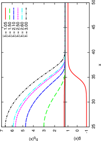
b)

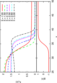
Figure 9: Top panels: Stationary solutions $h_{0}(x)$ (a)) and critical eigenfunction $h_{1}(x)$ (b)) for $\rho=0.5$ and different mean film heights $\mathrm{bar}h$. At $2.5<\mathrm{bar}h<2.6$, the transition between a unimodal and a bimodal shape occurs. Bottom panels: The inhomogeneity function $g(x)$, given by Eq. (III.2).

Figure 10: Maximal growth rates $\beta_{\text{max}}$ and the corresponding $q_{\text{max}}$, which are defined in Eq. (9), against $\mathrm{bar}h$ for a) $\rho=0.5$ and b) $\rho=0.3$.

For very thin films ($\mathrm{bar}h<\mathrm{bar}h_{1}$), the one-dimensional solutions are not yet droplets. They are better described by piecewise flat films with a higher mean film thickness on the MWS (cf. solution for $\mathrm{bar}h=1.05$ in Fig. 9 a)). The flat film pieces are sufficiently thin to be below the instability threshold for spinodal dewetting on respective homogeneous substrates. Therefore, the piecewise flat film solutions are stable, also in two dimensions.

For $\mathrm{bar}h_{1}<\mathrm{bar}h<\mathrm{bar}h_{2}$, the one-dimensional solutions have a pronounced droplet shape (cf. solution for $\mathrm{bar}h=1.5$ in Fig. 9 a)). The corresponding two-dimensional ridge solutions are not stable, but this instability is not the Rayleigh-Plateau-like instability that leads to the formation of bulges. This can be inferred from the shape of the critical eigenfunction $h_{1}(x)$, which is depicted in Fig. 9 b) for different $\mathrm{bar}h$. For a Rayleigh-Plateau-like instability, $h_{1}(x)$ is supposed to have two symmetric maxima corresponding to the broadening of the ridge (cf. Fig. 11).

Figure 11: Comparison of transversal instabilities with a unimodal eigenfunction $h_{1}(x)$ for small film heights (top, $\mathrm{bar}h=1.5$) and a bimodal $h_{1}(x)$ for larger film heights (bottom, $\mathrm{bar}h=3.0$). Shown are the steady ridge profiles (solid curves) together with the sum of the ridge profile and the eigenfunction multiplied by a small constant $\delta$ (dashed curve). In the first case the contact line stays fixed, in the second case it is shifted.

In the region $\mathrm{bar}h_{1}<\mathrm{bar}h<\mathrm{bar}h_{2}$, however, the function $h_{1}(x)$ has only one maximum. Therefore this instability is related to the formation of droplets on the MWS and therefore belongs to the growth regimes I to III observed in the experiments, which are sketched in Fig. 2.

In the region $\mathrm{bar}h_{2}<\mathrm{bar}h<\mathrm{bar}h_{3}$ the critical eigenfunction still has only one maximum, but the growth rates are negative for finite wavenumbers (and zero for $q=0$). In this region a ridge on the MWS is stable because it is no longer possible for the ridge to form droplets on the MWS. This can be seen from the critical eigenfunction at $\mathrm{bar}h=2.1$ in Fig. 9 b). It becomes broader than the MWS. Since in this region it is not yet energetically favorable for the ridge to leave the stripe, the ridge stabilizes. This corresponds to the growth regime V seen in the experiments.

For mean film heights above $\mathrm{bar}h_{3}$ it becomes energetically favorable for the liquid to cover also part of the LWS and the maximal growth rate becomes positive (cf. Fig. 10 (a)). At a critical film thickness of $\mathrm{bar}h^{*}\approx 2.5$, slightly greater than $\mathrm{bar}h_{3}\approx 2.4$, the critical eigenfunction undergoes a shape transition from unimodal to bimodal (see Fig. 11). The resulting instability is the Rayleigh-Plateau-like instability that leads to the formation of bulges. Therefore, the region $\mathrm{bar}h>\mathrm{bar}h_{3}$ corresponds to the growth regime VI (cf. Fig. 2).

For small wettability contrasts ($\rho\lesssim 0.43$) we observe the same shape transition in the critical eigenmode, but the maximal growth rate remains positive for $\mathrm{bar}h$ above the curve in Fig. 8. This is demonstrated in Fig. 10 (b) for $\rho=0.3$.

As a next step we take a look at the influence of the sharpness of the wettability transition. The dotted line in Fig. 8 shows the stability threshold in the $[\rho,\mathrm{bar}h]$ plane for $l_{s}=0.001$, i. e. for a sharper wettability transition. In this case, stable ridges are possible for lower wettability contrasts $\rho$. On the other hand, for $\rho\gtrsim 0.57$, the onset of the Rayleigh-Plateau instability is shifted towards lower $\mathrm{bar}h$. This is probably due to the fact that the effective width of the MWS decreases with decreasing $l_{s}$. Further decreasing $l_{s}$ does not lead to a significant change of the diagram, therefore $l_{s}=0.001$ can already be seen as the limiting case of a true step function.

Finally, we remark that the instability threshold in Fig. 8 reaches the value $\mathrm{bar}h\approx 1.26$ at $\rho=0$ as is the case for the sinusoidal wettability modulation in Fig. 5 above. This value of $\mathrm{bar}h\approx 1.26$ corresponds, as it should be, to the analytically obtained threshold of the spinodal instability of a flat film, which is given by $\partial\varPi/\partial h=0$. This reinforces the interpretation that the first instability for small $\rho$ and $\mathrm{bar}h$ is a spinodal instability. As one increases $\rho$ from zero to a small finite values while keeping $\mathrm{bar}h$ constant, the one-dimensional flat film solutions change towards more and more pronounced droplet solutions with increasing maximal film heights. This explains why the instability threshold with respect to $\mathrm{bar}h$ decreases with increasing $\rho$.

III.3 Comparison of diffusive and convective transport

Equation (5), which determines the equilibrium morphologies, does not depend on the mobility term $Q(h)$ as long as it is non-zero, whereas in the eigenvalue equation (III.1) only $Q(h_{0})$ enters. Hence, the mobility has an effect on the absolute values of $\beta$ when $\beta\neq 0$, but does not influence the position of the instability thresholds $\beta=0$ in parameter space. This is demonstrated in Fig. 12, where we plot, as in Fig. 10 (a), the maximum of the dispersion relation $\beta_{max}$ against the mean film height $\mathrm{bar}h$ for convective and diffusive mobility functions $Q(h)\sim h^{3}$ and $Q(h)\sim h$, respectively (note the semi-log scale in the upper panel). Although the absolute values are dramatically smaller for the diffusive mobility $Q(h)=h$, the stability thresholds $\beta_{max}=0$ remain at the same position, as can be seen more clearly in the bottom panel, where the corresponding $q_{max}$ is shown as a function of $\mathrm{bar}h$.

Figure 12: a) Maximal growth rates of the transversal instability for $\rho=0.5$ against $\mathrm{bar}h$. The dotted line corresponds to a convective mobility $Q(h)=h^{3}$. This curve is the same as in Fig. 10 a), but in logarithmic scaling. The solid line corresponds to a diffusive mobility term $h$. b) The corresponding fastest growing wavenumbers. The growth rates are significantly larger for the convective instability, especially in the bulge formation regime. The fastest growing wavenumbers are almost identical for both mobilities.

Therefore, we argue that the specific mobility that results from the particular dominant transport process(es) does neither influence the linear stability of the ridges nor the observed equilibrium morphologies. Only the time scales at which the instabilities grow depend on the mobility. This point will be further elucidated in the subsequent section where we consider the time evolution in the fully nonlinear regime.

IV Time simulations

In the previous section we have shown that there exist two different types of transversal instabilities that can occur in different ranges of values of the wettability contrast $\rho$: Inspection of the respective eigenfunctions indicates that for small volume a ridge decays into droplets that only cover the MWS, whereas for large volumes bulges evolve that also cover part of the LWS. Depending on the value of $\rho$ the two instabilities can be separated by a range of stable ridges. In the present section we test whether this finding of the linear analysis holds in the fully nonliner regime by performing direct numerical simulations of Eq. (1) in the two parameter regimes.

The numerical simulations are performed employing the alternating direction implicit (ADI) method. Thereby the spatial and time derivatives are discretised using second-order finite differences. This results in a nonlinear system of equations that is solved at each time step using Newton’s method. In each Newton iteration a linear system (Jacobian matrix of the nonlinear system) is efficiently solved employing the ADI method ( see Ref. 60; 31 for more details).

The first simulation is performed at low volume, for $\mathrm{bar}h=1.16$. This value corresponds to the maximum of $\beta_{max}$ that coincides to the maximum of $q_{max}$ (cf. Fig. 10 a)), in order to minimize the necessary computation time and domain size. The latter is then selected as $50$ in $x$- and $100$ in $y$-direction.

In the course of the time evolution we measure the non-dimensional free energy
$F(t)=\int\mathrm{d}x\,\mathrm{d}y\left[\tfrac{1}{2}(\nabla h)^{2}+f(h,\,x)\right]$, where $f(h,\,x)$ now stands for the non-dimensional wetting potential. Note that the total time derivative of the free energy is given by $\dfrac{dF}{dt}=-\int Q(h)\,\left(\dfrac{\delta F}{\delta h}\right)^{2}\,\mathrm{d}x\,\mathrm{d}y\,.$ As the mobility function $Q(h)$ is always positive, the final expression is negative, i.e., $F$ is a Lyapunov functional. As a consequence, linearly stable and unstable steady solutions of the thin film equation correspond to local minima or saddle points of the free energy functional $F$, respectively. The resulting dependency of energy on time is shown in Fig. 13.

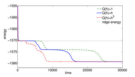
Figure 13: Time series of the energy during a direct numerical simulation of the thin film equation (1) with $\mathrm{bar}h=1.16$ for transport by surface diffusion (mobility $Q(h)\sim 1$, dash-dotted green curve), by bulk diffusion ($Q(h)\sim h$, solid blue line), and by convection ($Q(h)\sim h^{3}$, dashed red line). The configurations that correspond to the four energy plateaus for $Q(h)=h^{3}$ are plotted in Fig. 14.

In this energy time series obtained with the convective mobility function $Q(h)$ (dashed red curve) one can identify four plateaus of different length where the evolution approaches different steady states of the system. The first three correspond to unstable steady profiles, while the final one corresponds to the absolutely stable steady state configuration. All four configurations for $Q(h)=h^{3}$ are depicted in Fig. 14.

a) $t=10^{3}$	b) $t=3\cdot 10^{3}$
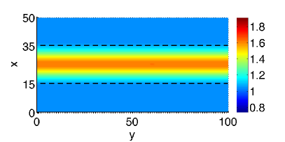
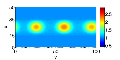
c) $t=6\cdot 10^{3}$	d) $t=10^{4}$

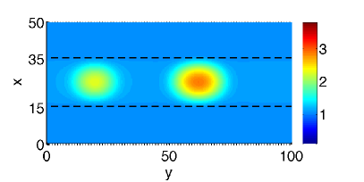
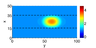
Figure 14: Snapshots of a direct time simulation of the thin film equation (1) with $\mathrm{bar}h=1.16$, $l_{s}=0.03$, $x_{A}=0.3$, $L_{per}=50$ in the case of purely convective transport (mobility $Q(h)=h^{3}$). The borders of the MWS is indicated by dashed (black) lines. Figure 13 shows the corresponding time series of the energy $F(t)$. The four snapshots at times $t=1000,\,3000,\,6000,\,10000$ correspond to the four energy plateaus in Fig. 13.

The first configuration, which is assumed very quickly starting from a flat film perturbed by small-amplitude noise, is a transversally invariant ridge that is identical to the one obtained above through one-dimensional steady state continuation. In Fig. 14 a) and Fig. 15, the solutions resulting from the direct numerical simulation (dotted line) and of the one-dimensional continuation (solid line) are compared.

Figure 15: Comparison between solutions that result from the one-dimensional continuation (solid line) and from the direct time simulation (where the dotted line gives the profile of a cross-section at $y=0$ and $t=1000$ of the transversally invariant ridge state assumed for a long intervall in the time evolution, cf. Fig. 14 a)).

The fact that this unstable steady state is assumed for a considerably long time during the time simulation retrospectively justifies the approach of the transversal linear stability analysis of the previous section. After a certain time the homogeneous ridge develops transversal modulations that grow exponentially and evolve into the three droplet state that corresponds to the second plateau and is depicted in Fig. 14 b). Two of the drops shrink and vanish in subsequent coarsening events until only one droplet remains (Fig. 14 c) and d)). The borders between the LWS and MWS in Fig. 14 are indicated by dashed black lines. From this one can see that the droplets are completely located on the MWS, in agreement with the experimental case (I) and with the discussion in the previous section.

Figure 16: The solid line gives $\log|F(t)-F_{0}|$, where $F_{0}$ is the free energy of the steady transversally invariant ridge state $h_{0}$ and $F(t)$ is the free energy at time $t$ during the time simulation in Fig. 14. The dashed curve shows the exponential growth with a growth rate $2\beta_{m}$ that one expects from the linear stability analysis w.r.t. transversal modes.

To further characterize the departure of the time evolution from the ridge state of the first plateau, Fig. 16 (solid line) shows the time evolution of the logarithm of the difference $\bigtriangleup F$ between the energy $F(t)$ and the reference energy $F_{0}$ of the ridge solution $h=h_{0}(\mathbf{x})$. One observes that for the time interval when the system is close to the unstable ridge solution (cf. Fig. 14 a) and b)), the energy $\bigtriangleup F$ grows exponentially with a growth rate $2\,\beta_{\mathrm{max}}$ (dashed curve) as expected from the transversal linear stability analysis. Here, $\beta_{\mathrm{max}}=\beta(q_{\mathrm{max}})$ is the growth rate, calculated for the most unstable mode of the transversally invariant ridge solution. Indeed, an expansion of the energy $F(t)$ about the ridge solution $h_{0}$ with the perturbed solution of the form $h=h_{0}+\varepsilon\,h_{1}(\mathbf{x})\,\exp(\beta\,t)$ reads

$$F(t) = F_{0}+\varepsilon\,\int\,d\mathbf{x}\,\frac{\delta F}{\delta h}\biggl{|}_{h=h_{0}}h_{1}(\mathbf{x})\,e^{\beta\,t}$$

$$+\varepsilon^{2}\,\int\,d\mathbf{x}\,\frac{\delta^{2}F}{\delta h^{2}}\biggl{|}_{h=h_{0}}h_{1}(\mathbf{x})^{2}\,e^{2\,\beta\,t}+\mathrm{h.\,o.\,t.}\,.$$

As the linear part in $\varepsilon$ of this expansion vanishes at $h=h_{0}$, the nontrivial term of lowest order is the quadratic one, explaining the growth rate of $2\,\beta$.

Note that the transient behaviour of the energy $F(t)$ changes when employing different mobility functions $Q(h)$. The solid blue and green dash-dotted lines in Fig. 13) give the result for linear (bulk diffusion) and constant (surface diffusion) mobilities, respectively. Remarkably, one clearly sees that the same energy plateaus appear independent of the chosen mobility, however, their relative duration depends on the particular chosen transport behaviour. For instance, with the convective mobility after the ridge configuration, the evolution visits the three drop solution that is still visible as a shoulder with the linear mobility and is only barely visible (when zooming in) with the constant mobility. The two drop solution is clearly visited by all evolutions and the final configuration (corresponding to the single drop solution) is the same for all mobilities $Q(h)$ what is expected as $F$ is a Lyapunov functional, independent of the mobility.

a) $t=10^{4}$	b) $t=2\cdot 10^{4}$
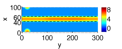
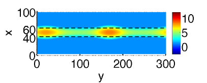
c) $t=3\cdot 10^{4}$	d) $t=8\cdot 10^{5}$

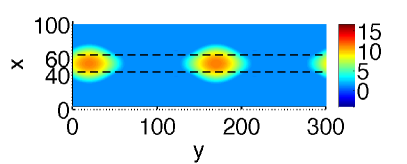
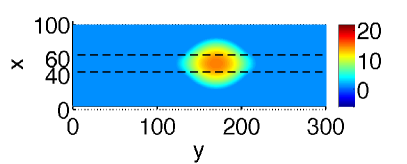
Figure 17: Snapshots of a direct time simulation of Eq. (1) at $h=1.9$, $\rho=0.5$, $l_{s}=0.015$, $x_{A}=0.4$ and $L_{per}=100$ and a convective mobility $Q(h)=h^{3}$. Panels (a), (b), (c), and (d) show snapshots at times $t=10^{4}$, $t=2\cdot 10^{4}$, $t=3\cdot 10^{4}$ and $t=8\cdot 10^{5}$, respectively. The borders of the more wettable stripes (MWS) is indicated by dashed (black) lines.

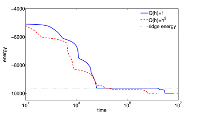
Figure 18: Time series of the free energy during the time simulation of Eq (1) with $\mathrm{bar}h=1.9$ for transport by surface diffusion (mobility $Q(h)\sim 1$, solid blue line) and by convection ($Q(h)\sim h^{3}$, dashed red line). The configurations that correspond to last four energy plateaus for $Q(h)=h^{3}$ are given in Fig. 17.

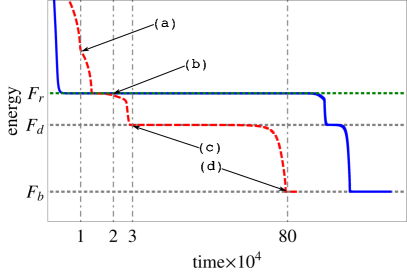
Figure 19: A zoom into the final thousand time steps in the energy plot (18) for the time simulation of Eq. (1) with $\mathrm{bar}h=1.9$ for transport by surface diffusion (mobility $Q(h)\sim 1$, solid blue line) and by convection ($Q(h)\sim h^{3}$, dashed red line). The letters (a)-(d) refer to snapshots from DNS (cf. Fig. 17) that correspond to last four energy plateaus for $Q(h)=h^{3}$ (right).

Next, we analyse the time evolution in the parameter range where, according to the linear stability analysis in the previous section, the second type of transversal instability should occur that is related to bulge formation. The wettability contrast is kept at $\rho=0.5$, but a larger initial film height $\mathrm{bar}{h}=1.9$ is chosen. Figure 17 shows four snapshots from this time simulation for a convective mobility $Q(h)=h^{3}$, whereas Fig. 18 gives the corresponding dependence of the energy on time for convective ($\sim h^{3}$, red dashed line) and surface diffusion ($\sim 1$, solid blue line) mobilities $Q(h)$). In addition, Fig. 19 shows a zoom into the energy evolution for the final thousand time steps (in logarithmic scale). There, the (a)-(d) letters correspond to the snapshots from the time simulations that correspond to the various plateaus. As in the previous case, the transversally invariant ridge is assumed quickly (Fig. 17 a)) and forms the starting point for the subsequent morphological transitions. Note, however, that here the ridge solution is accompanied by a single small drop, situated on the LWS. The existence of the state with this drop results in a shoulder in the energy plot at about $t=10^{4}$ (cf. Fig. 19). After a short time, the drop shrinks and disappears and the system stays close to the unstable steady transversally invariant ridge (with energy $F_{r}$) for some time (see the short energy plateau in Fig. 19 for $Q(h)=h^{3}$ close to $F_{r}$). Eventually the ridge develops modulations in $y$-direction (see panel b) of Fig. 17). These modulations grow and form two large bulges (Fig. 17 c) and Fig. 19 at $F=F_{d}$). Finally, one of them vanishes in a coarsening event and only one bulge remains (panel d) of Fig. 17 and Fig. 19 at $F=F_{b}$ ). From the dashed black line, indicating the borders of wettability regime, one can see that in this case the solution is not pinned to the MWS and also covers the LWS. The emerged configurations resemble the experimentally observed case VI (see Fig. 2.)

However, for larger initial film heights $\mathrm{bar}{h}$ the final bulge configuration itself (shown in Fig. 17 d)) can be unstable. Fig. 20 gives in panels a)-c) three snapshots from the time evolution for $\mathrm{bar}{h}=2.8$ with convective mobility $Q(h)=h^{3}$, while Fig. 20 d) shows the evolution of the energy $F(t)$ for convective transport (red dashed line) and for surface diffusion (blue solid line). As in the previous cases, the evolution visits similar unstable steady states until a state with two bulges is formed. However, this state does this time not only evolve via a coarsening event towards a single bulge, but at the same time forms a liquid bridge to the next MWS (the system is periodic in $y$-direction). The final liquid bridge state is shown in Fig. 20 c). However, the occurance of this final configuration strongly depends on the domain size and periodicity of the wettability pattern. A detailed investigation of this aspect is not within the scope of the current study and will be pursued elsewhere.

a) $t=10^{4}$

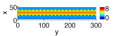
b) $t=5\cdot 10^{4}$

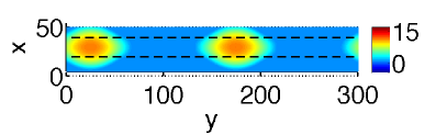
c) $t=1.5\cdot 10^{6}$

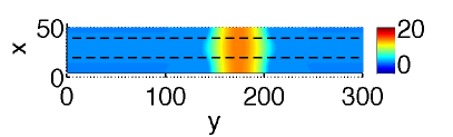
d)

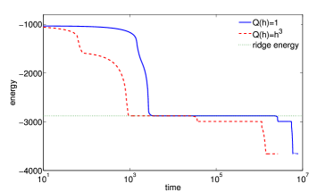
Figure 20: Snapshots from a direct time simulation of the thin film equation (1) with $\mathrm{bar}{h}=2.8$, $l_{s}=0.03$, $\rho=0.5$, $x_{A}=0.3$, and $L_{per}=50$. Panels a), b), c) show snapshots at times $t=10^{4}$, $t=5\cdot 10^{4}$ and $t=1.5\cdot 10^{6}$, respectively. The borders of the more wettable stripes (MWS) is indicated by dashed (black) lines. Panel d) shows time series of the energy $F(t)$ for transport by surface diffusion (mobility $Q(h)\sim 1$, solid blue line) and by convection ($Q(h)\sim h^{3}$, dashed red line).

V Conclusion

We have employed a mesoscopic continuum model to analyse the redistribution stage of deposition experiments where organic molecules are deposited by vapour deposition on a solid substrate with stripe-like wettability patterns. In particular, we have investigated the stability of transversally invariant ridges located on the more wettable parts of a stripe pattern by means of a linear stability analysis of steady one-dimensional profiles that correspond to the transversally invariant ridges on two-dimensional substrates. Employing a technique based on continuation procedures has allowed us to perform the linear analysis very efficiently. In particular, we have studied the influence of the wettability contrast, the mean film thickness (ridge volume), and the geometry of the stripe pattern.

We have found that there exist two different instability modes that on the one hand result at large ridge volume in the formation of bulges that spill from the more wettable stripes onto the less wettable bare substrate and on the one hand result at small ridge volume in the formation of small droplets located on the more wettable stripes, respectively. The different modes are reflected in qualitatively different eigenmodes that have their maxima in the regions of the strongest wettability gradient and at the stripe centre, respectively. They can be identified as a Rayleigh-Plateau instability and a surface instability as in spinodal dewetting, respectively.

In the parameter plane spanned by mean film height $\mathrm{bar}{h}$ (liquid volume) and wettability contrast $\rho$ one sees that a clear distinction between the two modes appears at some wettability contrast $\rho_{c}$. For $\rho>\rho_{c}$ two unstable film thickness ranges exist with a stable range of film thicknesses in between. The critical $\rho_{c}$ decreases with increasing steepness of the transition in wettability. In the opposite limit of a sinusoidal wettability pattern, i.e., when the transition zone is as wide as the period, no such distinction of two instability modes exists.

Further, we have investigated the role of the analysed transversally invariant ridge states in the course of the fully nonlinear time evolution starting from a deposited homogeneous film of molecules towards the final bulge or drop geometry. This has allowed us to assess whether a detailed analysis of ridge stability is meaningful in the context of deposition experiments with striped substrates. We have found that even linearly unstable ridge states form the first ’organising center’ of the time evolution. This is because they (as well as all other unstable states) represent saddles in the state space of the system. One may say that they ’attract’ time evolutions from the majority of directions in the infinite-dimensional space of system states and later ’expel’ them into one or a few directions and with rates that both can be determined by a linear stability analysis of the unstable states. In particular, the evolution that starts at a flat film with small perturbations is first attracted by the ridge state (the corresponding time scale is related to both, the most unstable eigenmode of the flat film and the slowest stable eigenmode of the ridge state. After ’visiting’ the transversally invariant ridge state the evolution is expelled along the single unstable direction in state space. It corresponds to the most unstable eigenmode of the ridge state (the corresponding time scale is the inverse of the growth rate of this eigenmode). The importance of the ridge state and also of the other unstable states (as, e.g., multidrop states) for the time evolution can be clearly seen in the formation of ’energy plateaus’ in all the plots that give the dependence of the free energy on time. Each plateau represents one of the unstable steady state. This observation is also important for other gradient dynamics systems as it indicates how important it is to understand the complete solution structure of a system in order to control its time evolution. It is further to expect that the unstable steady states are the ones that are most easily stabilized through imposed controls - be it spatial patterning or feedback.

The conclusion in the previous paragraph is strengthened by our finding that the relevance of the unstable states holds for all the different dominant transport mechanisms that we have investigated: the same energy plateaus appear independently of the chosen mobility, however, we have found that their relative duration depends on the particular chosen transport behaviour. This agrees with the fact discussed above that the steady states do not depend on mobilities, but that the time constants and eigenmodes do depend on them. As particular examples for the influence of the transport mechanism of redistribution on the evolution pathway, we have compared a standard long-wave hydrodynamic model in the case of no slip at the substrate (purely convective transport, cubic mobility) with diffusive transport via diffusion in the film bulk (linear mobility) and at the film surface (constant mobility). All the resulting long-wave evolution equations are gradient dynamics models on the identical underlying free energy (interface Hamiltonian) just with different mobility functions. As a result, one may now reconsider the film height evolution equation and combine thin film hydrodynamics for relatively thick layers and dynamical density functional theory for relatively thin layers by combining the corresponding mobilitiesnotb . This will allow one to investigate the cross-over between different dominant transport mechanisms depending on various parameters.

Based on our investigations we conclude more specifically that the different experimentally observed equilibrium morphologies do not result from the different transport mechanisms in the liquid or solid state as thought before. Instead, we have found that the observed flat and bulged deposits result from different balances of interface energies and wetting energies. The influence of bulk elastic energies may also play a role that shall be further investigated in the future.

Appendix A Appendix: Implementation in AUTO-07p

For the treatment with the continuation toolbox AUTO-07p, we have to transform Eqs. (5) and (III.1) into a system of first order ODEs on the interval $[0,1]$. To this end, we first define the independent variable $\xi:=x/L$ with $L$ denoting the physical domain size. Next, we introduce the variables

$$u_{1}(\xi) =h_{0}(L\xi)-\mathrm{bar}h~{},$$ (10)

$$u_{2}(\xi) =\left.\frac{\mathrm{d}h_{0}}{\mathrm{d}x}\right|_{x=L\xi}~{},$$ (11)

$$u_{3}(\xi) =h_{1}(L\xi)~{},$$ (12)

$$u_{4}(\xi) =\left.\frac{\mathrm{d}h_{1}}{\mathrm{d}x}\right|_{x=L\xi}~{},$$ (13)

$$u_{5}(\xi) =\left.\frac{\mathrm{d}^{2}h_{1}}{\mathrm{d}x^{2}}\right|_{x=L\xi}~{},$$ (14)

$$u_{6}(\xi) =\left.\frac{\mathrm{d}^{3}h_{1}}{\mathrm{d}x^{3}}\right|_{x=L\xi}~{},$$ (15)

$$u_{7}(\xi) =L\xi~{}.$$ (16)

Here, $\mathrm{bar}h$ denotes the mean film thickness. With the notation $\dot{u}_{i}(\xi)=\mathrm{d}u_{i}(\xi)/\mathrm{d}\xi$, the system of first order ODEs reads

$$\dot{u}_{1}= Lu_{2}$$ (17)

$$\dot{u}_{2}= -L[\varPi(\mathrm{bar}h+u_{1},u_{7})+C]$$ (18)

$$\dot{u}_{3}= Lu_{4}$$ (19)

$$\dot{u}_{4}= Lu_{5}$$ (20)

$$\dot{u}_{5}= Lu_{5}$$ (21)

$$\dot{u}_{6}= L\,\Big{\{}-\frac{\beta u_{3}}{Q_{0}}+q^{2}u_{5}-\partial_{x}^{2}(h_{1}\partial_{h}\varPi_{0})$$

$$-\frac{\partial_{x}Q_{0}}{Q_{0}}\,\left[(u_{6}-q^{2}u_{4}+\partial_{x}(h_{1}\partial_{h}\varPi_{0})\right]$$

$$+q^{2}\,\left[u_{5}-q^{2}u_{3}+\varPi^{\prime}(\mathrm{bar}{h}+u_{1})u_{3}\right]\Big{\}}$$ (22)

$$\dot{u}_{7}=L$$ (23)

with $Q_{0}=Q(u_{1}+\mathrm{bar}h)$ and

$$\partial_{x}(h_{1}\partial_{h}\varPi_{0})= ~{}\varPi^{\prime\prime}(\mathrm{bar}h+u_{1},u_{7})u_{2}u_{3}+\varPi^{\prime}(\mathrm{bar}h+u_{1},u_{7})u_{4}$$

$$+\varPi_{x}^{\prime}(\mathrm{bar}h+u_{1},u_{7})u_{3}~{},$$ (24)

$$\partial_{x}^{2}(h_{1}\partial_{h}\varPi_{0})= ~{}\varPi^{\prime\prime\prime}(\mathrm{bar}h+u_{1},u_{7})u_{2}^{2}u_{3}$$

$$+\varPi^{\prime\prime}(\mathrm{bar}h+u_{1},u_{7})(\partial_{x}^{2}h_{0})u_{3}$$

$$+2\varPi^{\prime\prime}(\mathrm{bar}h+u_{1},u_{7})u_{2}u_{4}$$

$$+\varPi^{\prime}(\mathrm{bar}h+u_{1},u_{7})u_{5}$$

$$+2\varPi^{\prime}_{x}(\mathrm{bar}h+u_{1},u_{7})u_{4}$$

$$+2\varPi^{\prime\prime}_{x}(\mathrm{bar}h+u_{1},u_{7})u_{2}u_{3}$$

$$+\varPi^{\prime}_{xx}(\mathrm{bar}h+u_{1},u_{7})u_{3}~{}.$$ (25)

In the last two equations, primes denote derivatives w. r. t. $h$ while the index $x$ means a derivative w. r. t. $x$ at constant $h$. The equation for $x=u_{7}$ is necessary because AUTO-07p only allows for autonomous ODEs.