No evidence for activity correlations in the radial velocities of Kapteyn’s star

Abstract

Stellar activity may induce Doppler variability at the level of a few m/s which can then be confused by the Doppler signal of an exoplanet orbiting the star. To first order, linear correlations between radial velocity measurements and activity indices have been proposed to account for any such correlation. The likely presence of two super-Earths orbiting Kapteyn’s star was reported in Anglada-Escudé et al. (2014), but this claim was recently challenged by Robertson et al. (2015b) arguing evidence of a rotation period (143 days) at three times the orbital period of one of the proposed planets (Kapteyn’s b, P=48.6 days), and the existence of strong linear correlations between its Doppler signal and activity data. By re-analyzing the data using global optimization methods and model comparison, we show that such claim is incorrect given that; 1) the choice of a rotation period at 143 days is unjustified, and 2) the presence of linear correlations is not supported by the data. We conclude that the radial velocity signals of Kapteyn’s star remain more simply explained by the presence of two super-Earth candidates orbiting it. We also advocate for the use of global optimization procedures and objective arguments, instead of claims lacking of a minimal statistical support.

1 Introduction

Recently, the search for low-amplitude signals in radial velocity time-series has reached the point where detection of Doppler signals at the level of 1m/s or less is technically possible (Pepe et al., 2011; Tuomi & Anglada-Escudé, 2013). Along with this rise in precision have come claims, and counter-claims, of the detection of planetary systems containing very low-mass planets (e.g. $\alpha$ Centauri, Dumusque et al., 2012, Hatzes, 2013; HD 41248 Jenkins et al., 2013; Jenkins & Tuomi, 2014, Santos et al., 2014; GJ 581 Mayor et al., 2009, Robertson et al., 2014, Anglada-Escudé & Tuomi, 2015). Given the sensitive nature of these works, it is clear more work must be done to develop a clear structure for what constitutes a Doppler signal detection and what does not.

It is known that stellar activity might induce spurious signals in precision Doppler measurements (Queloz et al., 2001, eg.). In particular, variability in chromospheric activity indices are supposed to originate from localized active regions on stars. Changes in the local properties of the visible surface of stars can induce apparent Doppler shifts that do not necessarily average out over time, producing apparent signals that might be mistaken as planets (eg. Hatzes, 2002; Bonfils et al., 2007). Theoretical and numerical simulations suggest that variability on some of these indices should linearly correlate with apparent radial velocity shifts (Boisse et al., 2011; Dumusque et al., 2014). Robertson et al. (2014) exploited this expected linear correlation to propose that the planet candidate GJ 581d was caused by stellar variability by showing some correlations of activity indices with residual time-series (all other signals removed). Since residual time-series are not representative of the original data, such conclusions were challenged by Anglada-Escudé & Tuomi (2015). In response, Robertson et al. (2015a) admitted inconsistencies in their statistical analysis but claimed that their interpretation of the data was physically more sound. Along these lines, in Robertson & Mahadevan (2014) and Robertson et al. (2015b) (RM15 hereafter) similar qualitative arguments were provided to argue that several super-Earth mass planet candidates orbiting nearby M-dwarf stars were likely to be spurious. In this paper we show that the claims in Robertson et al. (2015b) are unsupported by a global fit to the data, so such results should be regarded as inconclusive.

The data used in this paper comes directly from RM15 to replicate their setup as closely as possible. The datasets in RM15 contain measurements obtained with the HARPS and the HIRES spectrometers. These are different from the ones in Anglada-Escudé et al. (2014) in the sense that RM15 includes additional spectroscopic indices and, additionally, three HARPS epochs (out of 95) were removed. We also include the analysis of V magnitude historical photometric measurements obtained by the ASAS project (Pojmanski, 1997). A more detailed description of the measurements are given in both papers and references therein. We start by reviewing possible periodic signals in the activity indices presented by RM15 in Section 2. Section 3.1 introduces a minimal Doppler model to include linear correlation terms caused by activity. To remove ambiguities about the framework used, we perform the analyses in a frequentist (Section 3.2) and a Bayesian framework (Section 3.3); both providing a consistent picture of no correlations in either case. Section 4 discusses the discrepancy between our results and the analysis presented in RM15. A summary and concluding remarks are given in Section 5.

2 Possible signals in activity indices and ASAS photometry

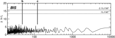
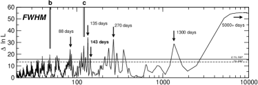
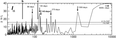
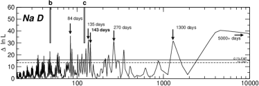
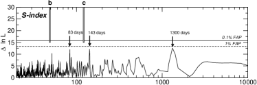
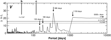
Figure 1: Likelihood periodograms of the activity indices in RM15 (from top to bottom; BIS, FWHM, $I_{\alpha}$, Na D, S-index) and ASAS V band photometry (bottom). With the exception of BIS, variability above 1% FAP threshold (horizontal line) is detected in all indices. Most relevant possible periods in each activity index are flagged with arrows. The similarities between periodograms in different indices (long period trend, and possible signals between 80 and 300 days) suggest similar, non-strictly periodic stellar variability in these time-ranges but does not point out to a clearly preferred signal.

We perform a likelihood periodogram analysis of the activity indices as provided by RM15 to verify the claim of a clear rotation period at 143 days. Likelihood ratio periodograms solves for all the free parameters of the model at the same time when a signal is injected over a list of trial periods (x-axis). Such periodograms are a generalization of Lomb-Scargle periodograms (Scargle, 1982) to account for models more complex than a single sinusoid (Baluev, 2009), including parameters of the noise model (eg. extra white noise for the activity data). The signal producing the highest improvement of the maximum log-likelihood statistic (y-axis) would be the preferred one and its significance can then be assessed using the recipes introduced by Baluev (2009, 2013), producing analytic estimates of the false alarm probability of detection (or FAP). As a general rule, signals above a FAP threshold of 1 % can be considered significant, but a more conservative threshold of 0.1% is sometimes used. We present both in all the periodograms presented throughout the paper. In the case of activity data, we assume that the signal is modelled by: one constant (equivalent to the mean of the time-series), one sinusoid (phase and amplitude are free parameters), and an extra white noise parameters added in quadrature to the nominal uncertainties of each measurement. As mentioned by RM15, nights with several measurements might be overweighted and bias the signal searches. To account for this, we present the analysis using night averages only (45 independent epochs). Our conclusions however didn’t differ substantially if all datapoints were included.

The activity indices provided in RM15 include BIS, FWHM, I_α, Na D, S-index. The first two are measurements of the shape of the mean spectral line (BIS and FWHM represent asymmetry and width respectively), which can potentially trace activity-induced features on the stellar photosphere. The last three ones are measurements of the chromospheric emission of the star at the H_α (I_α), Sodium D₁ and D₂ lines (Na D), and Calcium H+K lines (S-index). Chromospheric indices are also supposed to trace the presence of active regions on the star that might be responsible for apparent Doppler shifts. More precise definitions and possible connection to activity-induced signals are given in RM15 and references therein. The results of signal searches on the five indices used by RM15 (plus available V band photometry from the ASAS survey) are summarized in Figure 1.

No significant periodicity is detectable in BIS. Several other indices show multiple peaks above the 1% and 0.1% FAP thresholds (horizontal dashed and solid lines, respectively). However, several of the peaks have similar $\Delta$ ln-L values, meaning that they satisfy the data similarly well. The only exception is the long period trend (marked as 5000+ days in Fig 1), which in some cases produces a much larger improvement of the likelihood (eg. FWHM and $I_{\alpha}$; second and third panels from the top, respectively). Although the periodograms in RM15 also show a likely long period trend in several indices, this evidence was disregarded as irrelevant in RM15 by using generalistic arguments that are not supported by the literature. That is, most stars in the M-dwarf sub-sample of the HARPS-GTO program (Kapteyn’s star is part of it) were found to show chromospheric variability in similar indices over long time-scales by Gomes da Silva et al. (2012).

In summary, signals at 5000+, 1100, 270, 135 and 88 days would explain the activity data equally well (even better depending on the index). Given this ambiguity the preferred periods in the various activity indices, the choice made by RM15 for a rotation period at 143 days seems rather arbitrary.

3 Search for correlations in the Doppler data

3.1 Model

The next step in RM15’s analysis was to assess the significances of linear correlations of the Doppler signals with the activity indices. We implement linear correlations by adding a linear relationship between the radial velocities and activity data by using the following model

$$v(t)=M(\vec{\theta},t)+\sum_{i}c_{i}\,I_{i},$$ (1)

where $M$ contains all the Doppler variability modeled by Keplerian signals, and $\vec{\theta}$ lists the usual parameters used in RV modelling (see Tuomi & Anglada-Escudé, 2013, as an example). Activity measurements obtained simultaneous to $v(t)$ are I_i, where $i$ is added over all the activity indices under consideration. As discussed before, these indices include i=BIS, FWHM, I_α, Na D, S-index.

Given a model, one can search for the combination of parameters that optimize a figure of merit (global optimization), and then decide whether the inclusion of a correlation term or a planet is warranted given the improvement of the reference statistic. As long as global optimization is applied (all parameters adjusted simultaneously), there are various ways to assess significance of planetary signals or correlations using either Bayesian or frequentist approaches (Anglada-Escudé & Tuomi, 2012). A Bayesian approach consists of assessing which model has the highest probability given the data. Frequentist confidence tests evaluate the chances of obtaining an improvement of a statistic by an unfortunate combination of random errors. While RM15 show some apparent correlations when representing one Doppler signal against some of their activity data, the significance of those correlations was never established using model comparison. The next two sections show that the correlations claimed in RM15 are not significant when a global fit to the data is obtained in either framework.

3.2 Frequentist analysis

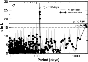
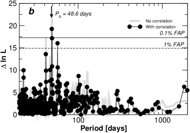
Figure 2: Likelihood-ratio periodograms for first (top, Kapteyn’s c, k=1 planet) and second Doppler signals (bottom, Kapteyn’s b, k=2 planets), without linear correlations (gray) and including linear correlations with the $I_{\alpha}$ index (connected black dots). The peaks for the Doppler signals remain above the 1% and 0.1% FAP thresholds in both cases.

In RM15, the strongest apparent correlation was reported to be in the chromospheric flux as measured by their $I_{\alpha}$ index. In Fig. 2 we present likelihood ratio periodograms of the combined HARPS and HIRES data (each data-set has its own linear correlation coefficient as a free parameter). As shown in Fig. 2, the significance of both signals (120 and 48.6 days) remain well above the 0.1% FAP threshold, even when linear correlations are included in the model. If linear correlations could explain the data better, adding a Keplerian signal would not improve the fit substantially and its peak would be suppressed below threshold. A similar result is obtained by using the other activity indices from RM15 (omited here for brevity). In summary, the likelihood analysis indicates that the linear correlation model cannot account for the presence either Doppler signals.

3.3 Bayesian analysis

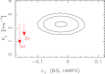
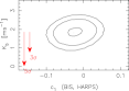
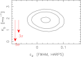
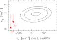
Figure 3: Posterior densities and equiprobability contours of the semi-amplitudes of the planet candidates $K_{c}$ (top) and $K_{b}$ (bottom) against the linear correlation terms defined in the text (x-axis). The contours contain 50%, 95%, and 99% of the probability density, respectively. The 3$\sigma$ and 5$\sigma$ intervals of the distributions are shown for $K_{b}$ and $K_{c}$ to demonstrate how significantly $K_{b}$ and $K_{c}$ differ from $0$. On the other hand, all $c_{i}$ are found to be broadly consistent with $0$.

In this section we perform a Bayesian analysis to evaluate the significance of correlations of the RV data with activity indices again assuming the linear model in Eq. 1. As before, we literally use the values provided in RM15 for simplicity in the discussion. All linear correlation terms ($c_{1}$ corresponds to HARPS BIS; $c_{2}$ to HARPS FWHM; $c_{3}$ to HARPS I_α; $c_{4}$ to HARPS Na D, and $c_{5}$ to the HARPS S-index) were tested at the same time by simultaneously including them all as free parameters. As a figure of merit for model comparison, we obtained the integrated likelihoods of models with and without signals and linear correlation terms. These integrated likelihoods (sometimes called Evidences $E$) were calculated by setting the priors as discussed in Tuomi & Anglada-Escudé (2013), and uniform ones for the parameters $c_{i}$. The algorithm used for the estimation of the integral is based on a mixture of Markov Chain Monte Carlo samples from both the posterior and prior (Newton et al., 1994).

Fig. 3 illustrates the posterior densities of each correlation coefficient c_i against the $K$ semi-amplitudes of the signals at 48.6 (Kapteyn’s b) and 120 days (Kapteyn’s c). The posterior densities were sampled using the adaptive-Metropolis posterior sampling algorithm (Haario et al., 2001). Two features would be expected for a radial velocity variations signal traced by an activity index. Firstly, the posterior densities in Fig. 3 would show a tilted elliptical shape and the value of the corresponding $c_{i}$ would be significantly different from $0$, and secondly, $K$ would be consistent with $0$ in the sense that 95% (or 99%) equiprobability contours overlapped with zero. Some of the plots show some mild hints of correlation (tilted ellipses), but all distributions for the $c_{i}$ are broadly consistent with $0$ values. In contrast, the expected value for the semiamplitudes of Kapteyn b is distinct from $0$ at a $\sim$ 5$\sigma$ level (even higher for Kapteyn’s c), where $\sigma$ is the standard deviation in of the posterior density in each $K$ (see Fig 3). The reason for the apparent contradiction with the claims in RM15 is explained in the next section.

Table 1 summarizes the model probabilities with linear correlations and planet signals included. The evidence ratios between models with $k$ and $k-1$ signals remain well above any reasonable significance threshold (eg. model probabilities larger than the 150-1000 factors usually required to claim a confident detection). The models including linear correlations (right) have slightly better integrated probabilities than those without (left), but the improvement is only a factor of $\sim$ 12 when comparing the models with $k=2$. This negligible level of significance of correlated variability is again consistent with the confidence level contours of Fig. 3, which imply that all $c_{i}$ are compatible with $0$.

Table 1: Natural logarithms of the integrated model probabilties $E$ and their ratios.

Number of Planets	Keplerian only		Keplerian + correlations
k	$\ln E_{k}$	$\ln(E_{k}/E_{k-1})$	$\ln E_{k}$	$\ln(E_{k}/E_{k-1})$
0	-277.7	-	-273.6	-
1	-260.1	+17.6	-254.9	+18.7
2	-238.8	+21.3	-241.3	+13.6†

Note. — ^†As a reference, a $\ln(E_{k}/E_{k-1})$ of +13.6 indicates that the model with $k$ planets has a higher probability than a model with $k-1$ planets by a factor $e^{+13.6}=8.1\times 10^{5}$.

4 Origin of the correlation proposed by RM15

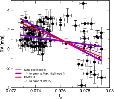
Figure 4: Correlation between the I_α index and the RVs once all signals except Kapteyn’s b have been removed from the data. The thin violet line is the maximum likelihood fit to the data we obtained, and the thick violet lines represent alternative fits within 1$\sigma$ values of the obtained correlation coefficient. The fit proposed by RM15 is represented by a red line and the 1$\sigma$ representations of their law are illustrated as dotted red lines.

There is a fundamental difference in the procedure we have used here to assess the presence of correlations and the one used by RM15. That is, while we used a global fit to the data to constrain the coefficients, RM15 used the predictions of the two planet model (with no errors) to perform their analysis. That is, RM15’s Figure 3 (top-central panel) shows $I_{\alpha}$ against the Doppler model of planet $b$. In our Figure 4, we show the same plot but present the radial velocity measurements after removing all signals except planet b. The linear correlation law derived from our Bayesian analysis in the previous section is presented in violet. Models showing allowed values of the correlation coefficients at $\pm$ 1$\sigma$ intervals are also represented as thick violet lines, which visually illustrates the large uncertainty in those. The best correlation law proposed by RM15 is shown as a red line, and red dotted lines show values of the coefficient at their reported $\pm$ 1$\sigma$ values. While the linear correlation law reported by RM15 is well within our 1$\sigma$ interval, their reported uncertainties are notoriously underestimated producing the spurious artifact of significant correlation. This is a direct consequence of misusing the RV model preductions (no uncertainties), instead of the actual data on testing the existence of potential correlation laws. We note for example, that even the Doppler model contains uncertainties, which where ignored in RM15.

5 Discussion

We have shown that linear correlations of RVs with activity indicators in the currently existing data are insignificant for Kapteyn’s star’s RVs when a global fit to the data is obtained. This stands in contrast to the claims made in RM15, which were based on a number of approximate physical assumptions and the implementation of ad hoc procedures. We also want to stress that interpretation of the 143d periodicity found by RM15 in several indicators as rotation period seems premature: alternative periods of 88d, 135d or 270d are similarly likely, and long-term activity trends cannot be ruled out either. Even If for the moment we assume that the star rotates at a period of 143d, it is not straightforward to use this as argument against a Doppler signal close-to $P_{rot}/3$, because there is no activity signal at $P_{rot}/2$ or $P_{rot}/3$. Given all these caveats, we consider that the current Doppler data of Kapteyn’s star is most easily explained by the presence of two planets as proposed in Anglada-Escudé et al. (2014) rather than activity induced variability as proposed by RM15.

A clear distinction must be made between the statistical significance of RV signals and the physical presence of planets (together with the merit of their detection or falsification). We advocate for comprehensive scientific discussions about the former instead of running into premature and unsupported statements about the latter. We conclude by emphasizing that the intention of this paper is not to rescue the planetary status of Kapteyn’s b or any other planet detection, but to stress the importance of objective global analysis techniques in serious scientific discussions.

References

- Anglada-Escudé & Tuomi (2012) Anglada-Escudé, G., & Tuomi, M. 2012, A&A, 548, A58
- Anglada-Escudé & Tuomi (2015) —. 2015, Science, 347, 1080
- Anglada-Escudé et al. (2014) Anglada-Escudé, G., Arriagada, P., Tuomi, M., et al. 2014, MNRAS, 443, L89
- Baluev (2009) Baluev, R. V. 2009, MNRAS, 393, 969
- Baluev (2013) —. 2013, MNRAS, 429, 2052
- Boisse et al. (2011) Boisse, I., Bouchy, F., Hébrard, G., et al. 2011, A&A, 528, A4
- Bonfils et al. (2007) Bonfils, X., Mayor, M., Delfosse, X., et al. 2007, A&A, 474, 293
- Dumusque et al. (2014) Dumusque, X., Boisse, I., & Santos, N. C. 2014, ApJ, 796, 132
- Dumusque et al. (2012) Dumusque, X., Pepe, F., Lovis, C., et al. 2012, Nature, 491, 207
- Gomes da Silva et al. (2012) Gomes da Silva, J., Santos, N. C., Bonfils, X., & et al. 2012, A&A, 541, A9
- Haario et al. (2001) Haario, H., Saksman, E., & Tamminen, J. 2001, Bernouilli, 7, 223
- Hatzes (2002) Hatzes, A. P. 2002, Astronomische Nachrichten, 323, 392
- Hatzes (2013) —. 2013, ApJ, 770, 133
- Jenkins & Tuomi (2014) Jenkins, J. S., & Tuomi, M. 2014, ApJ, 794, 110
- Jenkins et al. (2013) Jenkins, J. S., Tuomi, M., Brasser, R., Ivanyuk, O., & Murgas, F. 2013, ApJ, 771, 41
- Mayor et al. (2009) Mayor, M., Bonfils, X., Forveille, T., et al. 2009, A&A, 507, 487
- Newton et al. (1994) Newton, M. A., Raftery, A. E., & Probst, R. e. a. 1994, Journal of the Royal Statistical Society. Series B (Methodological), 56, 3
- Pepe et al. (2011) Pepe, F., Lovis, C., Ségransan, D., et al. 2011, A&A, 534, A58+
- Pojmanski (1997) Pojmanski, G. 1997, Acta Astron., 47, 467
- Queloz et al. (2001) Queloz, D., Henry, G. W., Sivan, J. P., et al. 2001, A&A, 379, 279
- Robertson & Mahadevan (2014) Robertson, P., & Mahadevan, S. 2014, ApJ, 793, L24
- Robertson et al. (2014) Robertson, P., Mahadevan, S., Endl, M., & Roy, A. 2014, Science, 345, 440
- Robertson et al. (2015a) —. 2015a, Science, 347, 1080
- Robertson et al. (2015b) Robertson, P., Roy, A., & Mahadevan, S. 2015b, ArXiv e-prints, arXiv:1505.02778
- Santos et al. (2014) Santos, N. C., Mortier, A., Faria, J. P., et al. 2014, A&A, 566, A35
- Scargle (1982) Scargle, J. D. 1982, ApJ, 263, 835
- Tuomi & Anglada-Escudé (2013) Tuomi, M., & Anglada-Escudé, G. 2013, A&A, 556, A111