t1t1footnotetext: This work was supported by the Deanship of Scientific Research at King Fahd University of Petroleum & Minerals (KFUPM) under Research Grant FT100030 and by the Viterbi fellowship from the Graduate School at the University of Southern California.t2t2footnotetext: Part of this work has appeared in the 13t​hsuperscript13π‘‘β„Ž13^{th} IEEE International Workshop on Signal Processing Advances in Wireless Communications (SPAWC 2012) [1].

Nonlinear Distortion Reduction in OFDM from Reliable Perturbations in Data Carriers

EbrahimΒ B.Β Al-Safadi alsafadi@usc.edu TareqΒ Y.Β Al-Naffouri tareq.alnaffouri@kaust.edu.sa MudassirΒ Masood mudassir.masood@kaust.edu.sa AnumΒ Ali anum.ali@kaust.edu.sa University of Southern California, Los Angeles, CA, United States. King Abdullah University of Science & Technology, Thuwal, Saudi Arabia. King Fahd University of Petroleum & Minerals, Dhahran, Saudi Arabia.
Abstract

A novel method for correcting the effect of nonlinear distortion in orthogonal frequency division multiplexing signals is proposed. The method depends on adaptively selecting the distortion over a subset of the data carriers, and then using tools from compressed sensing and sparse Bayesian recovery to estimate the distortion over the other carriers. Central to this method is the fact that carriers (or tones) are decoded with different levels of confidence, depending on a coupled function of the magnitude and phase of the distortion over each carrier, in addition to the respective channel strength. Moreover, as no pilots are required by this method, a significant improvement in terms of achievable rate can be achieved relative to previous work.

keywords:
OFDM, peak-to-average power ratio reduction, data-aided clipping mitigation, sparse Bayesian recovery, nonlinear distortion, compressed sensing.

1 Introduction

Multicarrier signaling schemes such as orthogonal frequency division multiplexing (OFDM) are highly susceptible to nonlinear distortion at all stages of the transmission process. This is partly due to the impulsive nature of these signals in the time domain, where the superposition of modulated waveforms takes place. When nonlinear distortion is confined to the transmitter, many proposed methods in the literature use reserved carriers (or tones) to carry information about this distortion to the receiver, at the obvious cost of reducing data-rate [2, 3, 4, 5]. The central idea in these techniques is to construct clipping (or peak-reducing) signals by performing a constrained search at the transmitter, one which confines the frequency support of the clipping signal to the reserved carriers, while reducing the peaks of the data signal in the time domain. These approaches are not generally robust, as they demand that the frequency support of the data and clipping signals remain strictly disjoint throughout the transmission process, and add significant complexity at the transmitter.

To combat this, techniques based on compressive sensing (CS) that were tuned to clipped OFDM models were proposed in [6]. These techniques removed the need for any constrained search at the transmitter, since the receiver could detect the entire clipping signal by observing a subset of its frequency components available on the reserved tones, provided that the signal is sparse in time. Consequently, the need to maintain orthogonality in frequency was completely relaxed, but the need for a significant amount of reserved carriers persisted. To avoid this loss in data-rate, the authors in [7] proposed using the channel estimation pilots for this purpose. Nonetheless, this approach severely limits the number of measurements available to the CS algorithm and hence its ability to deal with severe clipping scenarios. It also does not make use of available information such as clipping likelihood and phase resemblance in the time domain (i.e., phase resemblance between the clipped and clipping signal) as done in [6].

In this paper, a fundamentally different approach to these methods is pursued. Specifically, in contrast to the authors’ previous work on the topic of using CS concepts in OFDM [6], the technique presented in this paper does not require any orthogonality between the frequency support of the data and the distortion, and no tones (null, edge, channel pilots, or otherwise) are needed either. The receiver is free to select which and how many data tones it will use to read off differential observations, and will use them to estimate and cancel the entire distortion over the tones. In addition, no data-rate is lost by employing the proposed strategy. Furthermore, a significant tradeoff also exists in regard to complexity, distortion tolerance, and robustness to channel estimation errors, so that the user has many algorithms to use within the proposed framework. Similarly, in contrast to another recent work [1], the current paper introduces an entirely new and rigorous way of analyzing the reliability of tones. In addition, it also introduces a method to finetune the performance of CS by minimizing the probability of incorrect measurements and maximizing the clipping-to-noise ratio (CNR).

This framework is made possible by jointly taking three phenomena into account. The first is that not all tones carry correct decoding information to the receiver. The second is that the receiver can probabilistically assign levels of confidence to each tone, and the third is that the distortion is sparse in the time domain. These phenomena motivate us to employ CS and sparse recovery techniques much more effectively compared to previous techniques, as we can quantify the perturbations on data tones, select the most reliable ones, and then most-importantly, use the power of CS techniques to recover the significant time domain distortions. Our major contributions include:

  1. 1.

    Formulating CS models within a pilotless transmission framework.

  2. 2.

    Proposing systematic methods to adaptively select the tone subset to sense over, among the combinatorially large possibilities of pilotless CS models.

  3. 3.

    Developing a novel method for accurately assessing the reliability of estimated coefficients based on their symbol-wise magnitudes, phases, and relative locations to other constellation points, as well as channel strengths.

  4. 4.

    Deriving a closed-form expression that characterizes the modes of behavior of the reliability function, and devising geometrically-inspired approximations based on this expression for quick and efficient selection of the tone subset over each OFDM block.

  5. 5.

    Proposing dual-stage construction of the tone subset, where the first stage minimizes the probability of incorrect measurements, while the second maximizes an CNR metric to optimize CS performance.

  6. 6.

    Providing probabilistic upper bounds for choosing the number of tones in the CS model without risking incorrect measurements.

The remainder of the paper is organized as follows. Section 2 briefly describes the transmission and distortion models. Section 3 demonstrates how a pilotless CS model can be derived within the previous transmission model. Subsequently, Section 4, the heart of the paper, focuses on selecting the subset of tones used for CS. This includes developing reliability assessment criteria, deriving analytical approximations for quick and efficient assessment, selecting the number of tones, establishing dual-stage subset selection to maximize CS performance, and, finally, condensing the major results into an algorithm. Section 5 presents our simulations and Section 6 concludes the paper.

1.1 Notation

We use regular font for scalars and boldface letters for matrices and vectors. To distinguish between vectors in the time and frequency domains, we use boldface calligraphic notation for vectors in the frequency domain (e.g. 𝓧,𝓧¯,𝓨𝓧¯𝓧𝓨\mbox{$\bm{\mathcal{X}}$},\underline{\mbox{$\bm{\mathcal{X}}$}},\mbox{$\bm{\mathcal{Y}}$}) and boldface lowercase letters for their corresponding time domain representations (e.g. 𝒙,𝒙¯,π’šπ’™Β―π’™π’š{\bm{x}},\underline{{\bm{x}}},{\bm{y}}). We use 𝒳​(k)π’³π‘˜{\cal X}(k) to denote the kπ‘˜kth coefficient of 𝓧𝓧\bm{\mathcal{X}}, or more simply 𝒳𝒳{\cal X}, when it is clear from the context. Moreover, we use 𝓧Ωsubscript𝓧Ω\mbox{$\bm{\mathcal{X}}$}_{\Omega} to represent a vector formed by selecting the coefficients of 𝓧𝓧\bm{\mathcal{X}} indexed by set ΩΩ\Omega. Similarly, 𝓨Ωsubscript𝓨Ω\mbox{$\bm{\mathcal{Y}}$}_{\Omega} is the vector formed by indexing the corresponding elements of vector 𝓨Ωsubscript𝓨Ω\mbox{$\bm{\mathcal{Y}}$}_{\Omega} according to the index set ΩΩ\Omega. We further define 𝐒Ωsubscript𝐒Ω{\bf S}_{\Omega} to be a diagonal binary selection matrix, with |Ξ©|Ξ©|\Omega| number of 111’s at locations along its diagonal specified by the tone set ΩΩ\Omega.

2 Transmission and Clipping Model

In an OFDM system, serially incoming bits are mapped into an M𝑀M-ary QAM alphabet 𝓐={π’œ0,π’œ1,…,π’œMβˆ’1}𝓐subscriptπ’œ0subscriptπ’œ1…subscriptπ’œπ‘€1\mbox{$\bm{\mathcal{A}}$}\!=\!\{{\cal A}_{0},{\cal A}_{1},\ldots,{\cal A}_{M-1}\} and concatenated to form an N𝑁N-dimensional data vector, 𝓧=[𝒳​(0)​𝒳​(1),β‹―,𝒳​(Nβˆ’1)]π–³βˆˆπ“N𝓧superscript𝒳0𝒳1⋯𝒳𝑁1𝖳superscript𝓐𝑁\mbox{$\bm{\mathcal{X}}$}=[{\cal X}(0){\cal X}(1),\cdots,{\cal X}(N-1)]^{\sf T}\in\mbox{$\bm{\mathcal{A}}$}^{N}. The time domain signal 𝒙𝒙{\bm{x}} is obtained by an IFFT operation such that 𝒙=𝐅𝖧​𝓧𝒙superscript𝐅𝖧𝓧{\bm{x}}={\bf F}^{\sf H}\mbox{$\bm{\mathcal{X}}$}, where

Fk​(l)=Nβˆ’1/2​eβˆ’Θ·β€‹2​π​k​l/N,k,l∈0,1,…,Nβˆ’1.formulae-sequencesubscriptπΉπ‘˜π‘™superscript𝑁12superscript𝑒italic-Θ·2πœ‹π‘˜π‘™π‘π‘˜π‘™01…𝑁1F_{k}(l)=N^{-1/2}\,e^{-\jmath 2\pi kl/N},\quad k,l\in{0,1,\ldots,N-1}.

Since 𝒙𝒙{\bm{x}} has a high PAPR, the digital samples are subject to a magnitude limiter that saturates its operands to a value of γ𝛾\gamma. Hence, instead of 𝒙𝒙{\bm{x}}, we feed 𝒙¯¯𝒙\underline{{\bm{x}}} to the power amplifier, where

x¯​(i)={γ​eȷ​θx​(i)if​|x​(i)|>Ξ³,x​(i)otherwise,Β―π‘₯𝑖cases𝛾superscript𝑒italic-Θ·subscriptπœƒπ‘₯𝑖ifπ‘₯𝑖𝛾π‘₯𝑖otherwise\displaystyle\underline{x}(i)=\begin{cases}\gamma e^{\jmath\theta_{x(i)}}&\text{if}~{}|x(i)|>\gamma,\\ x(i)&\text{otherwise},\end{cases} (1)

and where ΞΈx​(i)subscriptπœƒπ‘₯𝑖\theta_{x(i)} is the phase of x​(i)π‘₯𝑖x(i). This hard-limiting operation can be conveniently thought of as adding a peak-reducing signal 𝒄𝒄{\bm{c}} to 𝒙𝒙{\bm{x}} so that its low-PAPR counterpart 𝒙¯=𝒙+𝒄¯𝒙𝒙𝒄\underline{{\bm{x}}}={\bm{x}}+{\bm{c}} is transmitted instead. Furthermore, by setting a typical clipping threshold, γ𝛾\gamma, on 𝒙𝒙{\bm{x}}, 𝒄𝒄{\bm{c}} is controllably sparse in time by the impulsive nature of 𝒙𝒙{\bm{x}}, and dense in frequency by the uncertainty principle. We denote the temporal support of 𝒄𝒄{\bm{c}} by ℐ𝒄={i:c​(i)β‰ 0}subscriptℐ𝒄conditional-set𝑖𝑐𝑖0{\cal I}_{{\bm{c}}}=\{i:c(i)\neq 0\} and always maintain the practical assumption that |ℐ𝒄|β‰ͺNmuch-less-thansubscriptℐ𝒄𝑁|{\cal I}_{{\bm{c}}}|\ll N.

Subsequently, 𝒙¯¯𝒙\underline{{\bm{x}}} is convolved with a channel of impulse response π’‰βˆΌπ’žβ€‹π’©β€‹(𝟎,σ𝒉2β€‹πˆL𝒉)similar-toπ’‰π’žπ’©0superscriptsubscriptπœŽπ’‰2subscript𝐈subscript𝐿𝒉{\bm{h}}\sim{\cal C}{\cal N}({\bf 0},\sigma_{{\bm{h}}}^{2}{\bf I}_{L_{{\bm{h}}}}), and subjected to additive white Gaussian noise (AWGN) π’›βˆΌπ’žβ€‹π’©β€‹(𝟎,σ𝒛2β€‹πˆN)similar-toπ’›π’žπ’©0superscriptsubscriptπœŽπ’›2subscriptπˆπ‘{\bm{z}}\sim{\cal C}{\cal N}({\bf 0},\sigma_{{\bm{z}}}^{2}{\bf I}_{N}), where LhsubscriptπΏβ„ŽL_{h} is the length of channel impulse response. Equivalently, in the frequency domain, this translates to transmitting

𝓧¯=𝓧+𝓒,¯𝓧𝓧𝓒\displaystyle\underline{\mbox{$\bm{\mathcal{X}}$}}\!=\!\mbox{$\bm{\mathcal{X}}$}+\mbox{$\bm{\mathcal{C}}$}, (2)

with complex coefficients that are now randomly pre-perturbed from the lattice 𝓐Nsuperscript𝓐𝑁\mbox{$\bm{\mathcal{A}}$}^{N}, followed by additional multiplicative perturbations by the channel 𝐇𝐇{\bf H} and additive perturbations by the noise π“©βˆΌπ’žβ€‹π’©β€‹(𝟎,σ𝒛2β€‹πˆN)similar-toπ“©π’žπ’©0superscriptsubscriptπœŽπ’›2subscriptπˆπ‘\mbox{$\bm{\mathcal{Z}}$}\sim{\cal C}{\cal N}({\bf 0},\sigma_{\bm{z}}^{2}{\bf I}_{N}) at the receiver. By virtue of the added cyclic prefix (of length >L𝒉absentsubscript𝐿𝒉>L_{{\bm{h}}}), the circulant channel matrix 𝐇𝐇{\bf H} can be decomposed and expressed as 𝐇=π…π–§β€‹πš²β€‹π…π‡superscriptπ…π–§πš²π…{\bf H}\!=\!{\bf F}^{\sf H}\hbox{\boldmath$\Lambda$}{\bf F} where 𝚲𝚲\Lambda is an NΓ—N𝑁𝑁N\times N diagonal matrix composed of the frequency-domain channel gains, {λ​(k)}k=1Nsuperscriptsubscriptπœ†π‘˜π‘˜1𝑁\{\lambda(k)\}_{k=1}^{N}. As a result the frequency domain received signal reads 𝓨=πš²β€‹π“§Β―+π“©π“¨πš²Β―π“§π“©\mbox{$\bm{\mathcal{Y}}$}=\hbox{\boldmath$\Lambda$}\underline{\mbox{$\bm{\mathcal{X}}$}}+\mbox{$\bm{\mathcal{Z}}$}, where, for the moment, we make the practical assumption that the channel coefficients are known at the receiver. Consequently, 𝓧¯¯𝓧\underline{\mbox{$\bm{\mathcal{X}}$}} can be directly recovered scalar-wise from 𝓨𝓨\bm{\mathcal{Y}}, i.e.,

𝒳¯^​(k)=Ξ»βˆ’1​(k)​𝒴​(k)=𝒳​(k)+π’žβ€‹(k)+Ξ»βˆ’1​(k)​𝒡​(k),^Β―π’³π‘˜superscriptπœ†1π‘˜π’΄π‘˜π’³π‘˜π’žπ‘˜superscriptπœ†1π‘˜π’΅π‘˜\displaystyle\hat{\underline{{\cal X}}}(k)=\lambda^{-1}(k){\cal Y}(k)={\cal X}(k)+{\cal C}(k)+\lambda^{-1}(k){\cal Z}(k), (3)

where we use the notation 𝒳^^𝒳\hat{{\cal X}} to represent the equalized estimate of 𝒳𝒳{\cal X} at the receiver. Writing (3) in vector notation yields

𝓧¯^=𝓧+𝓒+πš²βˆ’1​𝓩.^¯𝓧𝓧𝓒superscript𝚲1𝓩\displaystyle\hat{\underline{\mbox{$\bm{\mathcal{X}}$}}}=\mbox{$\bm{\mathcal{X}}$}+\mbox{$\bm{\mathcal{C}}$}+\hbox{\boldmath$\Lambda$}^{-1}\mbox{$\bm{\mathcal{Z}}$}. (4)

Let π’Ÿβ€‹(k)β‰œπ’žβ€‹(k)+Ξ»βˆ’1​(k)​𝒡​(k)β‰œπ’Ÿπ‘˜π’žπ‘˜superscriptπœ†1π‘˜π’΅π‘˜{\cal D}(k)\triangleq{\cal C}(k)+\lambda^{-1}(k){\cal Z}(k) denote the general distortion on 𝒳​(k)π’³π‘˜{\cal X}(k), We let fπ’Ÿsubscriptπ‘“π’Ÿf_{\cal D} to be the pdf of the general distortion π’Ÿπ’Ÿ{\cal D} which we assume to be zero mean circularly symmetric Gaussian with variance Οƒπ’Ÿ2superscriptsubscriptπœŽπ’Ÿ2\sigma_{\cal D}^{2}. (Please refer to Appendix A for details regarding the derivation of Οƒπ’Ÿ2superscriptsubscriptπœŽπ’Ÿ2\sigma_{\cal D}^{2}.) Equation (4) could now be written as

𝓧¯^=𝓧+𝓓.^¯𝓧𝓧𝓓\displaystyle\hat{\underline{\mbox{$\bm{\mathcal{X}}$}}}=\mbox{$\bm{\mathcal{X}}$}+\mbox{$\bm{\mathcal{D}}$}. (5)

Treating the clipping distortion as additive noise, an maximum likelihood (ML) decoder will recover 𝒳​(k)π’³π‘˜{\cal X}(k) by simply mapping 𝒳¯^​(k)^Β―π’³π‘˜\hat{\underline{{\cal X}}}(k) to the nearest constellation point111While π’œmsubscriptπ’œπ‘š{\cal A}_{m} refers to the mπ‘šmth constellation point (1≀m≀M)1π‘šπ‘€(1\!\leq\!m\!\leq\!M), we reserve βŸ¨π’³^​(k)⟩delimited-⟨⟩^π’³π‘˜\langle\hat{{\cal X}}(k)\rangle to denote the nearest constellation point corresponding to the kπ‘˜kth received data sample 𝒳^​(k)^π’³π‘˜\hat{{\cal X}}(k). Furthermore, note that the true constellation point corresponding to 𝒳^​(k)^π’³π‘˜\hat{{\cal X}}(k) is 𝒳​(k)π’³π‘˜{\cal X}(k). βŸ¨π’³Β―^​(k)⟩delimited-⟨⟩^Β―π’³π‘˜\langle\hat{\underline{{\cal X}}}(k)\rangle, where βŸ¨π’³Β―^​(k)βŸ©β‰œarg​minπ’œmβˆˆπ“β‘|𝒳¯^​(k)βˆ’π’œm|β‰œdelimited-⟨⟩^Β―π’³π‘˜argsubscriptsubscriptπ’œπ‘šπ“^Β―π’³π‘˜subscriptπ’œπ‘š\langle\hat{\underline{{\cal X}}}(k)\rangle\triangleq{\hbox{arg}}\min_{{\cal A}_{m}\in\bm{{\cal A}}}|\hat{\underline{{\cal X}}}(k)-{\cal A}_{m}|. In other words, the operation βŸ¨π’³^​(k)⟩delimited-⟨⟩^π’³π‘˜\langle\hat{{\cal X}}(k)\rangle corresponds to rounding 𝒳^​(k)^π’³π‘˜\hat{{\cal X}}(k) to the nearest constellation point. Note that βŸ¨π’³^​(k)⟩delimited-⟨⟩^π’³π‘˜\langle\hat{{\cal X}}(k)\rangle does not need to be the true constellation point, i.e., βŸ¨π’³^​(k)⟩delimited-⟨⟩^π’³π‘˜\langle\hat{{\cal X}}(k)\rangle might be different from 𝒳​(k)π’³π‘˜{\cal X}(k). Such a hard-decoding scheme is very efficient in the classical AWGN scenario for high signal-to-noise ratio (SNR). However, in our case, in addition to the additive noise Ξ»βˆ’1​(k)​𝒡​(k)superscriptπœ†1π‘˜π’΅π‘˜\lambda^{-1}(k){\cal Z}(k), we have a γ𝛾\gamma-dependent source of perturbation π’žβ€‹(k)π’žπ‘˜{\cal C}(k) which is independent of the SNR. CS and similar sparse recovery algorithms seem to be a very sensible solution towards recovery of π’žβ€‹(k)π’žπ‘˜{\cal C}(k). Since 𝒄𝒄{\bm{c}} is sparse in the time domain, a partial observation of 𝒄𝒄{\bm{c}} in frequency domain is sufficient to estimate 𝒄𝒄{\bm{c}} and hence 𝓒𝓒\bm{\mathcal{C}} in one shot. This would certainly get around the problem of unreliable perturbations as CS algorithms, for instance, can be totally blind to them and still offer near optimal signal reconstruction under mild conditions [8]. The main issue is to decide which partial observation to use. This will be the topic of the following section.

3 Development of Compressive Sensing Models with No Tone Reservation

With the addition of the general distortion vector 𝓓𝓓\bm{\mathcal{D}} to the data vector 𝓧𝓧\bm{\mathcal{X}}, we expect that part of the data samples will be severely perturbed such that they fall out of their true decision regions. Let βŸ¨π’³β€‹(k)⟩delimited-βŸ¨βŸ©π’³π‘˜\langle{\cal X}(k)\rangle denote the decoded data sample corresponding to 𝒳​(k)π’³π‘˜{\cal X}(k), then the true decision region for 𝒳​(k)π’³π‘˜{\cal X}(k) is defined as β„šβ€‹(k)β‰œ{𝒳​(k)+π’°βˆˆβ„‚:βŸ¨π’³β€‹(k)+π’°βŸ©=𝒳​(k)}β‰œβ„šπ‘˜conditional-setπ’³π‘˜π’°β„‚delimited-βŸ¨βŸ©π’³π‘˜π’°π’³π‘˜\mathbb{Q}(k)\!\triangleq\!\{\,{\cal X}(k)+{\cal U}\!\in\!\mathbb{C}\!:\!\langle{\cal X}(k)+{\cal U}\rangle\!=\!{\cal X}(k)\} where 𝒰𝒰{\cal U} is a factor which when added to 𝒳​(k)π’³π‘˜{\cal X}(k) keeps it in its true decision region. Moreover, denote by Ξ©T={k∈Ω:βŸ¨π’³β€‹(k)+π’Ÿβ€‹(k)⟩=𝒳​(k)}subscriptΩ𝑇conditional-setπ‘˜Ξ©delimited-βŸ¨βŸ©π’³π‘˜π’Ÿπ‘˜π’³π‘˜\Omega_{T}\!=\!\{k\in\Omega\!:\!\langle{\cal X}(k)+{\cal D}(k)\rangle\!=\!{\cal X}(k)\} the subset of data tones in Ξ©={1,2,…,N}Ξ©12…𝑁\Omega=\{1,2,\ldots,N\} in which the perturbations do not cause data samples to cross their true decision regions. Let Ω¯T=Ξ©\Ξ©Tsubscript¯Ω𝑇\Ξ©subscriptΩ𝑇\bar{\Omega}_{T}=\Omega\backslash\Omega_{T} be its complement. Over the data tones of Ξ©TsubscriptΩ𝑇\Omega_{T}, the equality in βŸ¨π’³Β―β€‹(k)⟩=𝒳​(k)delimited-βŸ¨βŸ©Β―π’³π‘˜π’³π‘˜\langle\underline{{\cal X}}(k)\rangle={\cal X}(k) is true and hence from (2) and (5), 𝓓ΩT=𝓧¯^Ξ©Tβˆ’π“§Ξ©T=𝓧¯^Ξ©Tβˆ’βŸ¨π“§Β―^Ξ©T⟩subscript𝓓subscriptΩ𝑇subscriptΒ―^𝓧subscriptΩ𝑇subscript𝓧subscriptΩ𝑇subscriptΒ―^𝓧subscriptΩ𝑇delimited-⟨⟩subscriptΒ―^𝓧subscriptΩ𝑇\mbox{$\bm{\mathcal{D}}$}_{\Omega_{T}}=\underline{\hat{\mbox{$\bm{\mathcal{X}}$}}}_{\Omega_{T}}-\mbox{$\bm{\mathcal{X}}$}_{\Omega_{T}}=\underline{\hat{\mbox{$\bm{\mathcal{X}}$}}}_{\Omega_{T}}-\langle\underline{\hat{\mbox{$\bm{\mathcal{X}}$}}}_{\Omega_{T}}\rangle. This is not true at the complement set Ω¯Tsubscript¯Ω𝑇\bar{\Omega}_{T} at which 𝓓Ω¯T=𝓧¯^Ω¯Tβˆ’π“§Ξ©Β―T≠𝓧¯^Ω¯Tβˆ’βŸ¨π“§^Ω¯T⟩subscript𝓓subscript¯Ω𝑇subscriptΒ―^𝓧subscript¯Ω𝑇subscript𝓧subscript¯Ω𝑇subscriptΒ―^𝓧subscript¯Ω𝑇delimited-⟨⟩subscript^𝓧subscript¯Ω𝑇\mbox{$\bm{\mathcal{D}}$}_{\bar{\Omega}_{T}}=\underline{\hat{\mbox{$\bm{\mathcal{X}}$}}}_{\bar{\Omega}_{T}}-\mbox{$\bm{\mathcal{X}}$}_{\bar{\Omega}_{T}}\neq\underline{\hat{\mbox{$\bm{\mathcal{X}}$}}}_{\bar{\Omega}_{T}}-\langle\hat{\mbox{$\bm{\mathcal{X}}$}}_{\bar{\Omega}_{T}}\rangle. More generally, we can write

𝓓=𝐒ΩT​(𝓧¯^βˆ’βŸ¨π“§Β―^⟩)+𝐒Ω¯T​(𝓧¯^βˆ’π“§),𝓓subscript𝐒subscriptΩ𝑇¯^𝓧delimited-⟨⟩¯^𝓧subscript𝐒subscript¯Ω𝑇¯^𝓧𝓧\displaystyle\mbox{$\bm{\mathcal{D}}$}={\bf S}_{\Omega_{T}}\left(\underline{\hat{\mbox{$\bm{\mathcal{X}}$}}}-\langle\underline{\hat{\mbox{$\bm{\mathcal{X}}$}}}\rangle\right)+{\bf S}_{\bar{\Omega}_{T}}\left(\underline{\hat{\mbox{$\bm{\mathcal{X}}$}}}-\mbox{$\bm{\mathcal{X}}$}\right), (6)

where 𝐒ΩTsubscript𝐒subscriptΩ𝑇{\bf S}_{\Omega_{T}} is an NΓ—N𝑁𝑁N\!\times\!N diagonal binary selection matrix, with |Ξ©T|subscriptΩ𝑇|\Omega_{T}| number of 111’s at locations along its diagonal specified by the tone set Ξ©TsubscriptΩ𝑇\Omega_{T}. It extracts the elements of the vector 𝓧¯^βˆ’βŸ¨π“§Β―^⟩¯^𝓧delimited-⟨⟩¯^𝓧\underline{\hat{\mbox{$\bm{\mathcal{X}}$}}}-\langle\underline{\hat{\mbox{$\bm{\mathcal{X}}$}}}\rangle according to the tone set Ξ©TsubscriptΩ𝑇\Omega_{T} while nulling the others. The matrix 𝐒Ω¯Tsubscript𝐒subscript¯Ω𝑇{\bf S}_{\bar{\Omega}_{T}} is similarly defined with 111’s along the diagonal specified by the set Ω¯Tsubscript¯Ω𝑇\bar{\Omega}_{T}. It is easy to see that 𝐒ΩT​𝐒Ω¯T=𝟎subscript𝐒subscriptΩ𝑇subscript𝐒subscript¯Ω𝑇0{\bf S}_{\Omega_{T}}{\bf S}_{\bar{\Omega}_{T}}={\bf 0}. Practically speaking, Ξ©TsubscriptΩ𝑇\Omega_{T} constitutes the larger part of the tone set ΩΩ\Omega. An essential part of OFDM signal recovery obviously constitutes finding Ξ©TsubscriptΩ𝑇\Omega_{T} and correcting the distortions over Ω¯Tsubscript¯Ω𝑇\bar{\Omega}_{T} to finally reach the state Ξ©T=Ξ©subscriptΩ𝑇Ω\Omega_{T}=\Omega.

From (5) we have at the receiver,

𝓧¯^=𝓧+𝓓,Β―^𝓧𝓧𝓓\displaystyle\underline{\hat{\mbox{$\bm{\mathcal{X}}$}}}=\mbox{$\bm{\mathcal{X}}$}+\mbox{$\bm{\mathcal{D}}$}, (7)

which is the analog estimate 𝓧¯^Β―^𝓧\underline{\hat{\mbox{$\bm{\mathcal{X}}$}}} of the data vector 𝓧𝓧\bm{\mathcal{X}} affected by the distortion 𝓓𝓓\bm{\mathcal{D}}. We define π“”β‰œπ“§βˆ’βŸ¨π“§Β―^βŸ©β‰œπ“”π“§delimited-⟨⟩¯^𝓧\mbox{$\bm{\mathcal{E}}$}\triangleq\mbox{$\bm{\mathcal{X}}$}-\langle\underline{\hat{\mbox{$\bm{\mathcal{X}}$}}}\rangle to be a vector that is nonzero at locations where the decoded estimate at the receiver βŸ¨π“§Β―^⟩delimited-⟨⟩¯^𝓧\langle\underline{\hat{\mbox{$\bm{\mathcal{X}}$}}}\rangle differs from the data vector 𝓧𝓧\bm{\mathcal{X}}. From the discussion above, we see that

𝒳¯^​(k)βˆ’βŸ¨π’³Β―^​(k)⟩¯^π’³π‘˜delimited-⟨⟩¯^π’³π‘˜\displaystyle\underline{\hat{{\cal X}}}(k)-\langle\underline{\hat{{\cal X}}}(k)\rangle ={π’Ÿβ€‹(k),ifβ€‹βŸ¨π’³Β―^​(k)⟩=𝒳​(k)π’Ÿβ€‹(k)+ℰ​(k),ifβ€‹βŸ¨π’³Β―^​(k)βŸ©β‰ π’³β€‹(k)absentcasesπ’Ÿπ‘˜ifdelimited-⟨⟩¯^π’³π‘˜π’³π‘˜π’Ÿπ‘˜β„°π‘˜ifdelimited-⟨⟩¯^π’³π‘˜π’³π‘˜\displaystyle=\begin{cases}{\cal D}(k),&\text{if}~{}\langle\underline{\hat{{\cal X}}}(k)\rangle={\cal X}(k)\\ {\cal D}(k)+{\cal E}(k),&\text{if}~{}\langle\underline{\hat{{\cal X}}}(k)\rangle\neq{\cal X}(k)\end{cases} (8)

which allows us to write

𝐒ΩT​(𝓧¯^βˆ’βŸ¨π“§Β―^⟩)=𝐒ΩT​𝓓subscript𝐒subscriptΩ𝑇¯^𝓧delimited-⟨⟩¯^𝓧subscript𝐒subscriptΩ𝑇𝓓\displaystyle{\bf S}_{\Omega_{T}}(\underline{\hat{\mbox{$\bm{\mathcal{X}}$}}}-\langle\underline{\hat{\mbox{$\bm{\mathcal{X}}$}}}\rangle)={\bf S}_{\Omega_{T}}\mbox{$\bm{\mathcal{D}}$} (9)

Note that we do not require all of Ξ©TsubscriptΩ𝑇\Omega_{T} to recover 𝒄𝒄{\bm{c}}. Rather, we only require an arbitrary subset Ξ©mβŠ†Ξ©TβŠ†Ξ©subscriptΞ©π‘šsubscriptΩ𝑇Ω\Omega_{m}\subseteq\Omega_{T}\subseteq\Omega of cardinality mβ‰œ|Ξ©m|≀|Ξ©T|β‰œπ‘šsubscriptΞ©π‘šsubscriptΩ𝑇m\triangleq|\Omega_{m}|\leq|\Omega_{T}| to correctly recover 𝒄𝒄{\bm{c}} by CS (mπ‘šm and |Ξ©m|subscriptΞ©π‘š|\Omega_{m}| will be used interchangeably as appropriate to denote the number of measurements). As a result, we can replace the equation above with 𝐒Ωm​(𝓧¯^βˆ’βŸ¨π“§Β―^⟩)=𝐒Ωm​𝓓=𝐒Ωm​𝐅​𝒄+𝐒Ωmβ€‹πš²βˆ’1​𝓩subscript𝐒subscriptΞ©π‘šΒ―^𝓧delimited-⟨⟩¯^𝓧subscript𝐒subscriptΞ©π‘šπ““subscript𝐒subscriptΞ©π‘šπ…π’„subscript𝐒subscriptΞ©π‘šsuperscript𝚲1𝓩{\bf S}_{\Omega_{m}}(\underline{\hat{\mbox{$\bm{\mathcal{X}}$}}}-\langle\underline{\hat{\mbox{$\bm{\mathcal{X}}$}}}\rangle)={\bf S}_{\Omega_{m}}\mbox{$\bm{\mathcal{D}}$}={\bf S}_{\Omega_{m}}{\bf F}{\bm{c}}+{\bf S}_{\Omega_{m}}\hbox{\boldmath$\Lambda$}^{-1}\mbox{$\bm{\mathcal{Z}}$}, where 𝐒Ωmsubscript𝐒subscriptΞ©π‘š{\bf S}_{\Omega_{m}} is also a NΓ—N𝑁𝑁N\!\times\!N diagonal binary selection matrix defined in a similar way as 𝐒ΩTsubscript𝐒subscriptΩ𝑇{\bf S}_{\Omega_{T}} in the above. We write the above equation simply as π“¨β€²β‰œπšΏβ€‹π’„+π“©β€²β‰œsuperscriptπ“¨β€²πšΏπ’„superscript𝓩′\mbox{$\bm{\mathcal{Y}}$}^{\prime}\triangleq\hbox{\boldmath$\Psi$}{\bm{c}}+\mbox{$\bm{\mathcal{Z}}$}^{\prime}, where πšΏβ‰œπ’Ξ©mβ€‹π…β‰œπšΏsubscript𝐒subscriptΞ©π‘šπ…\hbox{\boldmath$\Psi$}\triangleq{\bf S}_{\Omega_{m}}{\bf F}, π“©β€²β‰œπ’Ξ©mβ€‹πš²βˆ’1β€‹π“©β‰œsuperscript𝓩′subscript𝐒subscriptΞ©π‘šsuperscript𝚲1𝓩\mbox{$\bm{\mathcal{Z}}$}^{\prime}\triangleq{\bf S}_{\Omega_{m}}\hbox{\boldmath$\Lambda$}^{-1}\mbox{$\bm{\mathcal{Z}}$}, and π“¨β€²β‰œπ’Ξ©m​(𝓧¯^βˆ’βŸ¨π“§Β―^⟩)β‰œsuperscript𝓨′subscript𝐒subscriptΞ©π‘šΒ―^𝓧delimited-⟨⟩¯^𝓧\mbox{$\bm{\mathcal{Y}}$}^{\prime}\triangleq{\bf S}_{\Omega_{m}}(\underline{\hat{\mbox{$\bm{\mathcal{X}}$}}}-\langle\underline{\hat{\mbox{$\bm{\mathcal{X}}$}}}\rangle) which denotes the observation vector of the differences over the tones in Ξ©msubscriptΞ©π‘š\Omega_{m}, nulled at the discarded measurements. This leads us to a pilotless CS model222The reason we stress that the CS model does not reduce transmission rate is that there have been previous alternate attempts by the authors [6] and others [7] to use compressive sensing in a tone-reservation setting which required significant reduction in data-rate.

𝓨Ωmβ€²=𝚿Ωm​𝒄+𝓩Ωmβ€².subscriptsuperscript𝓨′subscriptΞ©π‘šsubscript𝚿subscriptΞ©π‘šπ’„subscriptsuperscript𝓩′subscriptΞ©π‘š\displaystyle\mbox{$\bm{\mathcal{Y}}$}^{\prime}_{\Omega_{m}}=\hbox{\boldmath$\Psi$}_{\Omega_{m}}{\bm{c}}+\mbox{$\bm{\mathcal{Z}}$}^{\prime}_{\Omega_{m}}. (10)

where 𝓨Ωmβ€²subscriptsuperscript𝓨′subscriptΞ©π‘š\mbox{$\bm{\mathcal{Y}}$}^{\prime}_{\Omega_{m}} is the |Ξ©m|subscriptΞ©π‘š|\Omega_{m}|-dimensional vector composed of the nonzero coefficients in 𝓨′superscript𝓨′\mbox{$\bm{\mathcal{Y}}$}^{\prime}.

By inspecting (10), we notice that 𝒄𝒄{\bm{c}} is an N𝑁N-dimensional sparse vector in the time domain, corresponding to the difference between the time representations of the OFDM signal 𝒙𝒙{\bm{x}} and its clipped counterpart 𝒙¯¯𝒙\underline{{\bm{x}}}. The matrix 𝚿Ωmβˆˆβ„‚mΓ—Nsubscript𝚿subscriptΞ©π‘šsuperscriptβ„‚π‘šπ‘\hbox{\boldmath$\Psi$}_{\Omega_{m}}\!\!\in\!\mathbb{C}^{m\times N} is obtained by mπ‘šm random row extractions from the NΓ—N𝑁𝑁N\!\times\!N Fourier matrix according to Ξ©msubscriptΞ©π‘š\Omega_{m} (the cause of randomness is discussed later). The mπ‘šm-dimensional vector 𝓨Ωmβ€²subscriptsuperscript𝓨′subscriptΞ©π‘š\mbox{$\bm{\mathcal{Y}}$}^{\prime}_{\Omega_{m}} is the corresponding partial frequency-domain observation that we use to estimate 𝒄𝒄{\bm{c}}, contaminated by the Gaussian noise vector, 𝓩Ωmβ€²subscriptsuperscript𝓩′subscriptΞ©π‘š\mbox{$\bm{\mathcal{Z}}$}^{\prime}_{\Omega_{m}}.

This is a standard model in CS [8, 9]. Note however that the parametrization by Ξ©msubscriptΞ©π‘š\Omega_{m} actually defines a huge set of 2Nsuperscript2𝑁2^{N} possible models333The reason is that we do not know Ξ©msubscriptΞ©π‘š\Omega_{m} or even |Ξ©m|subscriptΞ©π‘š|\Omega_{m}| and so we might have to search over all the subsets of N𝑁N tones giving us a total of 2Nsuperscript2𝑁2^{N} models like (10) to choose from.. In the forthcoming sections we will discuss in detail how to determine a proper model from all these possibilities. For the time being, we assume that an appropriate Ξ©msubscriptΞ©π‘š\Omega_{m} is chosen, and 𝒄𝒄{\bm{c}} could therefore be recovered using any CS technique, be it convex programming, greedy pursuit, or iterative thresholding, and a very flexible region for tradeoff exists in regard to the performance and complexity of these techniques.

In this paper, we use two different schemes of CS to recover 𝒄𝒄{\bm{c}} from the developed CS model in (10), one from the convex relaxation group and the other from greedy pursuit methods. More specifically, the first is an adaptation of the least absolute shrinkage and selection operator (LASSO) [10] to this problem called the weighted and phase-augmented LASSO (WPAL) [6]. It incorporates phase information and clipping likelihood available from the data in the time-domain to improve distortion recovery performed in the frequency-domain. Specifically, we know that 𝒄𝒄{\bm{c}} is composed of just the clipped portions of the transmitted signal 𝒙¯¯𝒙\underline{{\bm{x}}}, so at clipping locations βˆ β€‹c​(k)=βˆ’βˆ β€‹x¯​(k)βˆ π‘π‘˜βˆ Β―π‘₯π‘˜\angle{c(k)}=-\angle{\underline{x}(k)}. We also know that the closer |x¯​(k)|Β―π‘₯π‘˜|\underline{x}(k)| to the value of the clipping threshold γ𝛾\gamma, the higher the likelihood that 𝒄𝒄{\bm{c}} had an active coefficient at kπ‘˜k. This additional information is incorporated in the CS algorithm in the form of weighting to improve its performance. Therefore, we define π’˜β‰œ||𝒙¯^|βˆ’Ξ³|π–³β‰œπ’˜superscriptΒ―^𝒙𝛾𝖳{\bm{w}}\triangleq||\underline{\hat{{\bm{x}}}}|-\gamma|^{\sf T} to be such a weighting vector to the β„“1subscriptβ„“1\ell_{1}-norm of 𝒄𝒄{\bm{c}} in the LASSO where 𝒙¯^Β―^𝒙\underline{\hat{{\bm{x}}}} refers to the estimated received clipped signal. We further define the diagonal phase matrix Θ^c=βˆ’exp⁑(diag​(Θ·β€‹πœ½π’™Β―^))subscript^Ξ˜π‘diagitalic-Θ·subscript𝜽¯^𝒙\hat{\Theta}_{c}\!=\!-\exp\left(\textmd{diag}(\jmath\hbox{\boldmath$\theta$}_{\underline{\hat{{\bm{x}}}}})\right) such that 𝒄WPAL=Θ^c​|𝒄WPAL|superscript𝒄WPALsubscript^Ξ˜π‘superscript𝒄WPAL{\bm{c}}^{\textmd{WPAL}}=\hat{\Theta}_{c}|{\bm{c}}^{\textmd{WPAL}}|. With these two variables defined, the optimization problem we solve becomes

|𝒄WPAL|=arg​min|𝒄|βˆˆβ„Nβ€‹π’˜π–³β€‹|𝒄|superscript𝒄WPAL𝒄superscriptℝ𝑁argsuperscriptπ’˜π–³π’„\displaystyle\!\!\!\!\!\!\!\!\!\!\!\!|\,{\bm{c}}^{\textmd{WPAL}}\,|=\underset{|{\bm{c}}|\in\mathbb{R}^{N}}{{\hbox{arg}}\min}\>\>{\bm{w}}^{\sf T}|{\bm{c}}|
s.t. ‖𝓨Ωmβ€²βˆ’πšΏΞ©mβ€‹πš―^𝒄​|𝒄|β€–22<Ο΅superscriptsubscriptnormsubscriptsuperscript𝓨′subscriptΞ©π‘šsubscript𝚿subscriptΞ©π‘šsubscript^πš―π’„π’„22italic-Ο΅\displaystyle\!\!\!\!\!\!\!\!\|\,\mbox{$\bm{\mathcal{Y}}$}^{\prime}_{\Omega_{m}}-\hbox{\boldmath$\Psi$}_{\Omega_{m}}\hat{\hbox{\boldmath$\Theta$}}_{{\bm{c}}}|{\bm{c}}|\,\|_{2}^{2}<\epsilon (11)

for some noise-dependent parameter Ο΅italic-Ο΅\epsilon. The other technique is the fast Bayesian matching pursuit (FBMP) by Schniter et al. [11] chosen for its superior performance and efficiency when a relatively large number of measurements is available, which is indeed the case compared to tone reservation cases proposed in [6] and [7].

Finally, once 𝒄CSsuperscript𝒄CS{\bm{c}}^{\textmd{CS}} - the CS estimate of 𝒄𝒄{\bm{c}} - has been obtained through any of the abovementioned schemes, we use (2) and (4) to obtain

𝓧^^𝓧\displaystyle\hat{\mbox{$\bm{\mathcal{X}}$}} =\displaystyle= 𝓧¯^βˆ’π…β€‹π’„CS=𝓧+[π“’βˆ’π“’CS]+πš²βˆ’1​𝓩¯^𝓧𝐅superscript𝒄CS𝓧delimited-[]𝓒superscript𝓒CSsuperscript𝚲1𝓩\displaystyle\underline{\hat{\mbox{$\bm{\mathcal{X}}$}}}-{\bf F}{\bm{c}}^{\textmd{CS}}=\mbox{$\bm{\mathcal{X}}$}+[\mbox{$\bm{\mathcal{C}}$}-\mbox{$\bm{\mathcal{C}}$}^{\textmd{CS}}]+\hbox{\boldmath$\Lambda$}^{-1}\mbox{$\bm{\mathcal{Z}}$} (12)
β‰œβ‰œ\displaystyle\triangleq 𝓧+𝓔CS+πš²βˆ’1β€‹π“©β‰œπ“§+𝚫,β‰œπ“§superscript𝓔CSsuperscript𝚲1π“©π“§πš«\displaystyle\mbox{$\bm{\mathcal{X}}$}+\mbox{$\bm{\mathcal{E}}$}^{\textmd{CS}}+\hbox{\boldmath$\Lambda$}^{-1}\mbox{$\bm{\mathcal{Z}}$}\triangleq\mbox{$\bm{\mathcal{X}}$}+\hbox{\boldmath$\Delta$},

where 𝓔CSβ‰œπ“’βˆ’π“’CSβ‰œsuperscript𝓔CS𝓒superscript𝓒CS\mbox{$\bm{\mathcal{E}}$}^{\textmd{CS}}\triangleq\mbox{$\bm{\mathcal{C}}$}-\mbox{$\bm{\mathcal{C}}$}^{\textmd{CS}} and πš«β‰œπ“”CS+πš²βˆ’1β€‹π“©β‰œπš«superscript𝓔CSsuperscript𝚲1𝓩\hbox{\boldmath$\Delta$}\triangleq\mbox{$\bm{\mathcal{E}}$}^{\textmd{CS}}+\hbox{\boldmath$\Lambda$}^{-1}\mbox{$\bm{\mathcal{Z}}$}. 𝓧^^𝓧\hat{\mbox{$\bm{\mathcal{X}}$}} could be used to determine the data vector 𝓧𝓧\bm{\mathcal{X}} exactly, provided that no Δ​(k)Ξ”π‘˜\Delta(k) causes crossing of 𝒳​(k)π’³π‘˜{\cal X}(k) out of its ML decoding region (this issue will come up in Section 4.3). Our subsequent objective is to scrutinize the general conditioning of the model itself by supplying our most reliable observations to the generic CS algorithm.

4 Cherry Picking Ξ©msubscriptΞ©π‘š\Omega_{m}

An essential question now is how to select among the 2Nsuperscript2𝑁2^{N} possible Ξ©msubscriptΞ©π‘š\Omega_{m} (or (Nm)binomialπ‘π‘šN\choose m if mπ‘šm is fixed) in order to compute 𝒄CSsuperscript𝒄CS{\bm{c}}^{\textmd{CS}}. In this connection we devise a reliability function which associates a reliability estimate with each tone and thus lets us determine the mπ‘šm most reliable tones to construct Ξ©msubscriptΞ©π‘š\Omega_{m}. A general strategy of CS techniques is to select these mπ‘šm tones randomly for near-optimal performance [8]. Although possible in our scenario, such a strategy neglects the fact that our observations vary in their credibility and attest to whether or not they represent true frequency-domain measurements of 𝓒𝓒\bm{\mathcal{C}}.444The measurements at tones Ξ©msubscriptΞ©π‘š\Omega_{m} in (11) are used to determine 𝒄𝒄{\bm{c}} and hence 𝓒𝓒\bm{\mathcal{C}}. However, these measurements truly represent 𝓒𝓒\bm{\mathcal{C}} only if βŸ¨π’³^​(k)⟩=𝒳​(k)delimited-⟨⟩^π’³π‘˜π’³π‘˜\langle\hat{{\cal X}}(k)\rangle={\cal X}(k) for k∈Ωmπ‘˜subscriptΞ©π‘šk\in\Omega_{m}. We can not ascertain that it is true but we can calculate its probability.

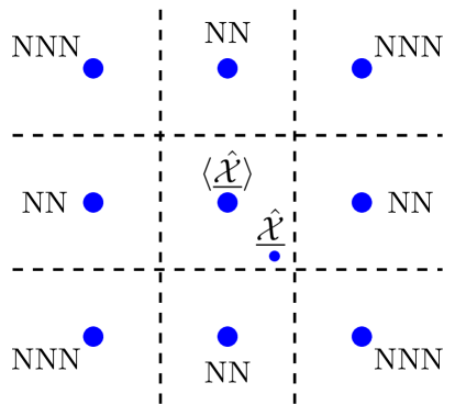
Since we deal with each tone separately in what follows, we henceforth drop the kπ‘˜k index while preserving the italic notation to emphasize the scalar-wise operations in this section. With the receiver risking faulty decisions, it must devise a procedure to select the most reliable set of observations over which to sense. To this end consider the estimate 𝒳¯^Β―^𝒳\underline{\hat{{{\cal X}}}} and the nearest constellation point βŸ¨π’³Β―^⟩delimited-⟨⟩¯^𝒳\langle\underline{\hat{{{\cal X}}}}\rangle. The latter is in general surrounded by eight points which either belong to the set of nearest neighbors (NN) or the set of next nearest neighbors (NNN) as illustrated in Fig.Β 1.

Refer to caption
Figure 1: An illustration of nearest neighbors (NN) and next nearest neighbors (NNN) of 𝒳¯^Β―^𝒳\underline{\hat{{\cal X}}}

Now the selection of the most reliable set of observations could be done based on the relative posterior probability that 𝓓𝓓\bm{\mathcal{D}} equals 𝒳¯^βˆ’βŸ¨π’³Β―^⟩¯^𝒳delimited-⟨⟩¯^𝒳\underline{\hat{{\cal X}}}-\langle\underline{\hat{{\cal X}}}\rangle to the probability that it equals some other difference vector 𝒳¯^βˆ’π’œm|π’œmβ‰ βŸ¨π’³Β―^⟩¯^𝒳conditionalsubscriptπ’œπ‘šsubscriptπ’œπ‘šdelimited-⟨⟩¯^𝒳\underline{\hat{{\cal X}}}-{\cal A}_{m}|{\cal A}_{m}\neq\langle\underline{\hat{{\cal X}}}\rangle. For example, let β„œ=Pr⁑(βŸ¨π’³Β―^⟩=𝒳)Pr⁑(βŸ¨π’³Β―^⟩=π’œNN)β„œPrdelimited-⟨⟩¯^𝒳𝒳Prdelimited-⟨⟩¯^𝒳subscriptπ’œNN\mathfrak{R}=\frac{\Pr(\langle\underline{\hat{{\cal X}}}\rangle={\cal X})}{\Pr(\langle\underline{\hat{{\cal X}}}\rangle={\cal A}_{\textmd{NN}})}. The higher the value of β„œβ„œ\mathfrak{R}, the higher the reliability that 𝒳=βŸ¨π’³^βŸ©π’³delimited-⟨⟩^𝒳{\cal X}=\langle\hat{{\cal X}}\rangle as relative to the fact that 𝒳^^𝒳\hat{{\cal X}} should decode to π’œN​Nsubscriptπ’œπ‘π‘{\cal A}_{NN}. From (7), we can see that β„œ=Pr⁑(π’Ÿ=𝒳¯^βˆ’βŸ¨π’³Β―^⟩)Pr⁑(π’Ÿ=𝒳¯^βˆ’π’œNN)β„œPrπ’ŸΒ―^𝒳delimited-⟨⟩^¯𝒳Prπ’Ÿ^¯𝒳subscriptπ’œNN\mathfrak{R}=\frac{\Pr({\cal D}=\underline{\hat{{\cal X}}}-\langle\hat{\underline{\mathcal{X}}}\rangle)}{\Pr(\mathcal{D}=\hat{\underline{\mathcal{X}}}-\mathcal{A}_{\textmd{NN}})}Now as mentioned earlier, we model π’Ÿπ’Ÿ{\cal D} to be Gaussian circularly symmetric with variance Οƒπ’Ÿ2superscriptsubscriptπœŽπ’Ÿ2\sigma_{{\cal D}}^{2}, then fπ’Ÿβ€‹(𝒳)=1Ο€β€‹Οƒπ’Ÿ2​exp⁑(βˆ’1Οƒπ’Ÿ2​|𝒳|2)subscriptπ‘“π’Ÿπ’³1πœ‹superscriptsubscriptπœŽπ’Ÿ21superscriptsubscriptπœŽπ’Ÿ2superscript𝒳2f_{\cal D}({\cal X})=\frac{1}{\pi\sigma_{\cal D}^{2}}\exp(-\frac{1}{\sigma_{\cal D}^{2}}|{\cal X}|^{2}) and we can write,

β„œβ„œ\displaystyle\mathfrak{R}\! =\displaystyle= exp⁑(βˆ’1ΟƒD2​(|𝒳¯^βˆ’βŸ¨π’³Β―^⟩|2βˆ’|𝒳¯^βˆ’π’œNN|2))1superscriptsubscript𝜎𝐷2superscriptΒ―^𝒳delimited-⟨⟩¯^𝒳2superscriptΒ―^𝒳subscriptπ’œNN2\displaystyle\!\exp{\left(\frac{-1}{\sigma_{D}^{2}}\left(|\underline{\hat{{\cal X}}}-\langle\underline{\hat{{\cal X}}}\rangle|^{2}-|\underline{\hat{{\cal X}}}-{\cal A}_{\textmd{NN}}|^{2}\right)\right)}

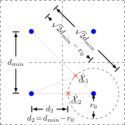
Intuitively, the minimum certainty occurs at the boundary of the decision region and attains β„œmin=1subscriptβ„œ1\mathfrak{R}_{\min}=1. At such tones, we would be highly skeptical of whether π’Ÿ=𝒳¯^βˆ’βŸ¨π’³Β―^βŸ©π’ŸΒ―^𝒳delimited-⟨⟩¯^𝒳{\cal D}=\underline{\hat{{\cal X}}}-\langle\underline{\hat{{\cal X}}}\rangle or π’Ÿ=𝒳¯^βˆ’π’œNNπ’ŸΒ―^𝒳subscriptπ’œNN{\cal D}=\underline{\hat{{\cal X}}}-{\cal A}_{\textmd{NN}}, and we would hence supply a plausibly false measurement to the CS algorithm. To avoid such unreliable measurements, assume we only choose the tones with respective perturbations 𝒳¯^βˆ’βŸ¨π’³Β―^⟩¯^𝒳delimited-⟨⟩¯^𝒳\underline{\hat{{\cal X}}}-\langle\underline{\hat{{\cal X}}}\rangle that are confined in the complex plane to a disk of radius rosubscriptπ‘Ÿπ‘œr_{o} (i.e., |𝒳¯^βˆ’βŸ¨π’³Β―^⟩|≀ro^¯𝒳delimited-⟨⟩¯^𝒳subscriptπ‘Ÿπ‘œ|\hat{\underline{{\cal X}}}-\langle\underline{\hat{{\cal X}}}\rangle|\leq r_{o}). In such a case, given the minimum distance between any two constellation points (dminsubscript𝑑d_{\min}), the minimum reliability would increase to β„œmin=fπ’Ÿβ€‹(ro)fπ’Ÿβ€‹(dminβˆ’ro)subscriptβ„œsubscriptπ‘“π’Ÿsubscriptπ‘Ÿπ‘œsubscriptπ‘“π’Ÿsubscript𝑑subscriptπ‘Ÿπ‘œ\mathfrak{R}_{\min}=\frac{f_{{\cal D}}(r_{o})}{f_{{\cal D}}(d_{\min}-r_{o})} in case the complex scalar 𝒳¯^βˆ’βŸ¨π’³Β―^⟩¯^𝒳delimited-⟨⟩¯^𝒳\underline{\hat{{\cal X}}}-\langle\underline{\hat{{\cal X}}}\rangle pointed in the direction of the nearest neighbor π’œNNsubscriptπ’œNN{\cal A}_{\textmd{NN}}, and to β„œ=fπ’Ÿβ€‹(ro)fπ’Ÿβ€‹(2​dminβˆ’ro)β„œsubscriptπ‘“π’Ÿsubscriptπ‘Ÿπ‘œsubscriptπ‘“π’Ÿ2subscript𝑑subscriptπ‘Ÿπ‘œ\mathfrak{R}=\frac{f_{{\cal D}}(r_{o})}{f_{\mathcal{D}}\left(\sqrt{2}d_{\min}-r_{o}\right)} for the next nearest neighbor π’œNNNsubscriptπ’œNNN{\cal A}_{\textmd{NNN}} when it points in the direction of a decision region’s corner. So while both 𝒳^1subscript^𝒳1\hat{{\cal X}}_{1} and 𝒳^2subscript^𝒳2\hat{{\cal X}}_{2} have the same distance rosubscriptπ‘Ÿπ‘œr_{o} from βŸ¨π’³^1⟩=βŸ¨π’³^2⟩delimited-⟨⟩subscript^𝒳1delimited-⟨⟩subscript^𝒳2\langle\hat{{\cal X}}_{1}\rangle=\langle\hat{{\cal X}}_{2}\rangle, 𝒳^1subscript^𝒳1\hat{{\cal X}}_{1} has a higher reliability than 𝒳^2subscript^𝒳2\hat{{\cal X}}_{2} as it is farther from the nearest neighbor. Fig.Β 2 shows a part of constellation to illustrate the idea. This suggests a need to factor in the direction or phase of the perturbation, θ𝒳¯^βˆ’βŸ¨π’³Β―^⟩subscriptπœƒΒ―^𝒳delimited-⟨⟩¯^𝒳\theta_{\underline{\hat{{\cal X}}}-\langle\underline{\hat{{\cal X}}}\rangle}, in assessing its reliability in addition to the magnitude-dependent pdf fπ’Ÿsubscriptπ‘“π’Ÿf_{{\cal D}}. Defined axiomatically, the reliability of a measurement at each tone is then a function β„œβ„œ\mathfrak{R} that maps a 333-tuple (|𝒳¯^βˆ’βŸ¨π’³Β―^⟩|,θ𝒳¯^βˆ’βŸ¨π’³Β―^⟩,Ξ»βˆ’1)Β―^𝒳delimited-⟨⟩¯^𝒳subscriptπœƒ^¯𝒳delimited-⟨⟩¯^𝒳superscriptπœ†1(|\underline{\hat{{\cal X}}}-\langle\underline{\hat{{\cal X}}}\rangle|,\theta_{\hat{\underline{{\cal X}}}-\langle\underline{\hat{{\cal X}}}\rangle},\lambda^{-1}) into ℝ[1,∞]subscriptℝ1\mathbb{R}_{[1,\infty]} (i.e., a function of the magnitude of the observation, its phase and the channel gain at that tone).
Refer to caption
Figure 2: Reliability is not only a function of the magnitude but also the phase of the observation.

Ultimately, we would choose our measurements according to the tones associated with the highest mπ‘šm reliability outputs, i.e.,

Ξ©mβ‰œarg​{β„œi:N}i=Nβˆ’m+1Nβ‰œsubscriptΞ©π‘šargsuperscriptsubscriptsubscriptβ„œ:π‘–π‘π‘–π‘π‘š1𝑁\displaystyle\Omega_{m}\triangleq{\hbox{arg}}\left\{\mathfrak{R}_{i:N}\right\}_{i=N-m+1}^{N} (13)

to sense over, where β„œi:Nsubscriptβ„œ:𝑖𝑁\mathfrak{R}_{i:N} denotes the i𝑖ith-order statistic in the vector 𝕽𝕽\bm{\mathfrak{R}} [12]. With this selection of Ξ©msubscriptΞ©π‘š\Omega_{m}, the locations of the measurement tones correspond to the indices of the highest mπ‘šm-order statistics of N𝑁N random variables in 𝕽𝕽\bm{\mathfrak{R}}. As mentioned previously, each of these variables is a function of the 333-tuple above, and whereas the first two are uncorrelated across the tones, this does not generally hold for the third, i.e., λ​(k)πœ†π‘˜\lambda(k).

In fact, assuming L𝒉subscript𝐿𝒉L_{{\bm{h}}} channel taps with a uniform power-delay profile, then the absolute autocorrelation of the channel across tones kπ‘˜k and l𝑙l can be expressed as |𝔼​[λ​(k)​λH​(l)]|=sinc​(π​L𝒉​(kβˆ’l)/N)𝔼delimited-[]πœ†π‘˜superscriptπœ†π»π‘™sincπœ‹subscriptπΏπ’‰π‘˜π‘™π‘|\mathbb{E}[\lambda(k)\lambda^{H}(l)]|=\textmd{sinc}\left(\pi L_{{\bm{h}}}(k-l)/N\right) [13]. Hence, only for sufficiently large L𝒉subscript𝐿𝒉L_{{\bm{h}}} can we assume that the channel gains are uncorrelated. Otherwise, the set of reliable tones Ξ©msubscriptΞ©π‘š\Omega_{m} deviates from a uniformly random tone selection model typically assumed in the literature [8, 9], and reliable tones would instead come in clusters corresponding to strong channel gains. The efficiency of CS in this case might be reduced555Nonetheless some methods such as FBMP are not much hindered by this fact [11]..

4.1 Criteria for Evaluating β„œβ„œ\mathfrak{R}

Using the reasoning based on the scalar-wise likelihood ratio defined in (4), an exact expression for the reliability could be a direct generalization of (4), namely,

β„œexact=fπ’Ÿβ€‹(𝓧¯^βˆ’βŸ¨π“§Β―^⟩)βˆ‘m=0,π’œmβ‰ βŸ¨π’³Β―^⟩Mβˆ’1fπ’Ÿβ€‹(𝒳¯^βˆ’π’œm),superscriptβ„œexactsubscriptπ‘“π’ŸΒ―^𝓧delimited-⟨⟩¯^𝓧superscriptsubscriptformulae-sequenceπ‘š0subscriptπ’œπ‘šdelimited-⟨⟩¯^𝒳𝑀1subscriptπ‘“π’ŸΒ―^𝒳subscriptπ’œπ‘š\displaystyle\mathfrak{R}^{\text{exact}}=\frac{f_{{\cal D}}(\underline{\hat{\mbox{$\bm{\mathcal{X}}$}}}-\langle\underline{\hat{\mbox{$\bm{\mathcal{X}}$}}}\rangle)}{\sum_{{m=0,{\cal A}_{m}\neq\langle\underline{\hat{{\cal X}}}\rangle}}^{M-1}f_{{\cal D}}(\underline{\hat{{\cal X}}}-{\cal A}_{m})}, (14)

Unfortunately, this pursuit for exact reliability computation is inefficient since it requires N​M𝑁𝑀N\!M evaluations of fπ’Ÿβ€‹(β‹…)subscriptπ‘“π’Ÿβ‹…f_{{\cal D}}(\cdot), which grows with the constellation size M𝑀M, even though the probability of a perturbation exceeding the first tier of eight surrounding neighbors (i.e., the nearest and next nearest neighbors illustrated in Fig. 1) is insignificant. As such, we can truncate the computation above to the first tier, denoting its result by β„œtruncsuperscriptβ„œtrunc\mathfrak{R}^{\textmd{trunc}}, with a minor effect on the performance.

Two simpler reliability functions are also worth mentioning. The first is solely based on the probability of the perturbation (i.e., fπ’Ÿβ€‹(|𝒳¯^βˆ’βŸ¨π’³Β―^⟩|)subscriptπ‘“π’Ÿ^¯𝒳delimited-⟨⟩¯^𝒳f_{{\cal D}}(|\hat{\underline{{\cal X}}}-\langle\underline{\hat{{\cal X}}}\rangle|)) and is hence completely blind to the direction of the perturbation in the constellation’s plane, while the other one intuitively takes this extra phase information into account by defining a square centered at βŸ¨π’³Β―^⟩delimited-⟨⟩¯^𝒳\langle\underline{\hat{{\cal X}}}\rangle as the reliable region, hence having the ability to favor perturbations with larger magnitudes if θ𝒳¯^βˆ’βŸ¨π’³Β―^⟩subscriptπœƒΒ―^𝒳delimited-⟨⟩¯^𝒳\theta_{\underline{\hat{{\cal X}}}-\langle\underline{\hat{{\cal X}}}\rangle} were close to Ο€/4πœ‹4\pi/4, i.e., if they pointed to the next nearest neighbor. We denote these reliability functions by β„œβˆ˜superscriptβ„œ\mathfrak{R}^{\circ} and β„œβ–‘superscriptβ„œβ–‘\mathfrak{R}^{\Box}, respectively, motivated by the geometric shape they define. In the next section, a more rigorous approach is taken to justify when such simpler methods can be used.

4.2 Analysis of Truncated and Approximate Reliability Criteria

Dropping the tone index, assume that 𝒳¯^Β―^𝒳\underline{\hat{{\cal X}}} is an observation that falls among four points in an M𝑀M-QAM constellation such that 𝒳¯^βˆˆβ„šΒ―^π’³β„š\underline{\hat{{\cal X}}}\in\mathbb{Q}. Let 𝒳¯^βˆ’βŸ¨π’³Β―^βŸ©β‰œr​eΘ·β€‹ΞΈβ‰œΒ―^𝒳delimited-⟨⟩¯^π’³π‘Ÿsuperscript𝑒italic-Θ·πœƒ\underline{\hat{{\cal X}}}-\langle\underline{\hat{{\cal X}}}\rangle\triangleq re^{\jmath\theta} be the polar representation of this point with the origin at βŸ¨π’³Β―^⟩delimited-⟨⟩¯^𝒳\langle\underline{\hat{{\cal X}}}\rangle, such that rβ‰œ|𝒳¯^βˆ’βŸ¨π’³Β―^⟩|∈[0,12​dmin]β‰œπ‘ŸΒ―^𝒳delimited-⟨⟩¯^𝒳012subscript𝑑r\triangleq|\underline{\hat{{\cal X}}}-\langle\underline{\hat{{\cal X}}}\rangle|\in[0,\frac{1}{\sqrt{2}}d_{\min}] and ΞΈβ‰œΞΈπ’³Β―^βˆ’βŸ¨π’³Β―^⟩∈[0,Ο€/2]β‰œπœƒsubscriptπœƒΒ―^𝒳delimited-⟨⟩¯^𝒳0πœ‹2\theta\triangleq\theta_{\underline{\hat{{\cal X}}}-\langle\underline{\hat{{\cal X}}}\rangle}\in[0,\pi/2]. We are interested in a more abstract expression of the truncated Bayesian reliability function, β„œtruncsuperscriptβ„œtrunc\mathfrak{R}^{\textmd{trunc}}, one that defines its output by only acting on 𝒳¯^βˆ’βŸ¨π’³Β―^⟩¯^𝒳delimited-⟨⟩¯^𝒳\underline{\hat{{\cal X}}}-\langle\underline{\hat{{\cal X}}}\rangle while taking the relative position in the constellation implicitly into account as well666This could be similarly carried out to the non-truncated function (14) albeit with an unnecessary inflation of expressions with hardly any additional insight..

By the definition of rπ‘Ÿr, and by referring to Fig.Β 3 which again shows a part of the constellation diagram (similar to Fig.Β 2), the distances between 𝒳¯^Β―^𝒳\underline{\hat{{\cal X}}} and the other three competing constellation points are

r1​(r,ΞΈ)=r2βˆ’2​r​dmin​cos⁑θ+dmin2,subscriptπ‘Ÿ1π‘Ÿπœƒsuperscriptπ‘Ÿ22π‘Ÿsubscriptπ‘‘πœƒsuperscriptsubscript𝑑2\displaystyle r_{1}(r,\theta)=\sqrt{r^{2}-2rd_{\min}\cos\theta+d_{\min}^{2}}, (15)
r2​(r,ΞΈ)=r2βˆ’2​r​dmin​(cos⁑θ+sin⁑θ)+2​dmin2,subscriptπ‘Ÿ2π‘Ÿπœƒsuperscriptπ‘Ÿ22π‘Ÿsubscriptπ‘‘πœƒπœƒ2superscriptsubscript𝑑2\displaystyle r_{2}(r,\theta)=\sqrt{r^{2}-2rd_{\min}(\cos\theta+\sin\theta)+2d_{\min}^{2}}, (16)

and

r3​(r,ΞΈ)=r2βˆ’2​r​dmin​sin⁑θ+dmin2.subscriptπ‘Ÿ3π‘Ÿπœƒsuperscriptπ‘Ÿ22π‘Ÿsubscriptπ‘‘πœƒsuperscriptsubscript𝑑2\displaystyle r_{3}(r,\theta)=\sqrt{r^{2}-2rd_{\min}\sin\theta+d_{\min}^{2}}. (17)
Refer to caption
Figure 3: Defining all fπ’Ÿβ€‹(ri)subscriptπ‘“π’Ÿsubscriptπ‘Ÿπ‘–f_{\mathcal{D}}(r_{i}) in terms of rπ‘Ÿr and ΞΈπœƒ\theta.
Refer to caption
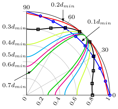
Figure 4: β„œtrunc​(r,ΞΈ)superscriptβ„œtruncπ‘Ÿπœƒ\mathfrak{R}^{\text{trunc}}(r,\theta) in (18) normalized and plotted on the first quadrant for Οƒπ’Ÿ2=0.2​dminsuperscriptsubscriptπœŽπ’Ÿ20.2subscript𝑑\sigma_{\mathcal{D}}^{2}\!=\!0.2d_{\min} and evaluated at r=0.1​dmin,0.2​dmin,π‘Ÿ0.1subscript𝑑0.2subscript𝑑r\!=0.1d_{\min},0.2d_{\min}, …,0.7​dmin…0.7subscript𝑑\ldots,0.7d_{\min}. Note that ΞΈπœƒ\theta varies from 0∘superscript00^{\circ} to 90∘superscript9090^{\circ}.

We neglect detailing their phases, ΞΈ1,ΞΈ2,subscriptπœƒ1subscriptπœƒ2\theta_{1},\theta_{2}, and ΞΈ3subscriptπœƒ3\theta_{3}, since they have no effect on the results, although r1,r2subscriptπ‘Ÿ1subscriptπ‘Ÿ2r_{1},r_{2}, and r3subscriptπ‘Ÿ3r_{3} are clearly functions of rπ‘Ÿr and ΞΈπœƒ\theta as portrayed in Fig. 3. In effect, β„œtruncsuperscriptβ„œtrunc\mathfrak{R}^{\textmd{trunc}} reduces to

β„œtrunc​(r,ΞΈ)=superscriptβ„œtruncπ‘Ÿπœƒabsent\displaystyle\mathfrak{R}^{\textmd{trunc}}(r,\theta)= fπ’Ÿβ€‹(r)/βˆ‘i=13fπ’Ÿβ€‹(ri​(r,ΞΈ))subscriptπ‘“π’Ÿπ‘Ÿsuperscriptsubscript𝑖13subscriptπ‘“π’Ÿsubscriptπ‘Ÿπ‘–π‘Ÿπœƒ\displaystyle f_{{\cal D}}(r)/\sum_{i=1}^{3}f_{{\cal D}}(r_{i}(r,\theta))
=\displaystyle= eβˆ’r2Οƒπ’Ÿ2/[eβˆ’1Οƒπ’Ÿ2​(r2βˆ’2​r​dmin​cos⁑θ+dmin2)+\displaystyle e^{\frac{-r^{2}}{\sigma_{{\cal D}}^{2}}}/\Big{[}e^{\frac{-1}{\sigma_{{\cal D}}^{2}}(r^{2}-2rd_{\min}\cos\theta+d_{\min}^{2})}+
eβˆ’1Οƒπ’Ÿ2​(r2βˆ’2​r​dmin​(cos⁑θ+sin⁑θ)+2​dmin2)+eβˆ’1Οƒπ’Ÿ2​(r2βˆ’2​r​dmin​sin⁑θ+dmin2)].\displaystyle e^{\frac{-1}{\sigma_{{\cal D}}^{2}}\left(r^{2}-2rd_{\min}\left(\cos\theta+\sin\theta\right)+2d_{\min}^{2}\right)}+e^{\frac{-1}{\sigma_{{\cal D}}^{2}}\left(r^{2}-2rd_{\min}\sin\theta+d_{\min}^{2}\right)}\Big{]}.

Canceling out the common function fπ’Ÿβ€‹(r)subscriptπ‘“π’Ÿπ‘Ÿf_{{\cal D}}(r) appearing in all terms above, and collecting common terms yields

β„œtrunc​(r,ΞΈ)superscriptβ„œtruncπ‘Ÿπœƒ\displaystyle\mathfrak{R}^{\textmd{trunc}}(r,\theta)\!\!\! =\displaystyle= (eβˆ’dmin2Οƒπ’Ÿ2​[e1Οƒπ’Ÿ2​(2​dmin​r​cos⁑θ)+e1Οƒπ’Ÿ2​(2​dmin​r​(cos⁑θ+sin⁑θ)βˆ’dmin2)+e1Οƒπ’Ÿ2​(2​dmin​r​sin⁑θ)])βˆ’1superscriptsuperscript𝑒superscriptsubscript𝑑2superscriptsubscriptπœŽπ’Ÿ2delimited-[]superscript𝑒1superscriptsubscriptπœŽπ’Ÿ22subscriptπ‘‘π‘Ÿπœƒsuperscript𝑒1superscriptsubscriptπœŽπ’Ÿ22subscriptπ‘‘π‘Ÿπœƒπœƒsuperscriptsubscript𝑑2superscript𝑒1superscriptsubscriptπœŽπ’Ÿ22subscriptπ‘‘π‘Ÿπœƒ1\displaystyle\!\!\!\Big{(}e^{-\frac{d_{\min}^{2}}{\sigma_{{\cal D}}^{2}}}[e^{\frac{1}{\sigma_{{\cal D}}^{2}}\left(2d_{\min}r\cos\theta\right)}+e^{\frac{1}{\sigma_{{\cal D}}^{2}}\left(2d_{\min}r\left(\cos\theta+\sin\theta\right)-d_{\min}^{2}\right)}+e^{\frac{1}{\sigma_{{\cal D}}^{2}}\left(2d_{\min}r\sin\theta\right)}]\Big{)}^{-1} (18)
β‰œβ‰œ\displaystyle\triangleq (β​[Ξ±cos⁑θ+Ξ±sin⁑θ+β​αcos⁑θ+sin⁑θ])βˆ’1superscript𝛽delimited-[]superscriptπ›Όπœƒsuperscriptπ›Όπœƒπ›½superscriptπ›Όπœƒπœƒ1\displaystyle\!\!\!\!\left(\beta\left[\alpha^{\cos\theta}\!+\!\alpha^{\sin\theta}\!+\!\beta\alpha^{\cos\theta+\sin\theta}\right]\right)^{-1}

for the first quadrant, θ∈[0,Ο€/2]πœƒ0πœ‹2\theta\in[0,\pi/2], in the complex plane, where Ξ±β‰œexp⁑(2​dmin​r/Οƒπ’Ÿ2)β‰œπ›Ό2subscriptπ‘‘π‘ŸsuperscriptsubscriptπœŽπ’Ÿ2\alpha\triangleq\exp(2d_{\min}r/\sigma_{{\cal D}}^{2}) and Ξ²β‰œexp⁑(βˆ’dmin2/Οƒπ’Ÿ2)β‰œπ›½superscriptsubscript𝑑2superscriptsubscriptπœŽπ’Ÿ2\beta\triangleq\exp(-d_{\min}^{2}/\sigma_{{\cal D}}^{2}). Although clearly a function of rπ‘Ÿr, we will treat α𝛼\alpha as a constant (i.e., evaluated at a fixed magnitude, rπ‘Ÿr) when we wish to focus on β„œtruncsuperscriptβ„œtrunc\mathfrak{R}^{\textmd{trunc}} as an explicit function of ΞΈπœƒ\theta, say g​(ΞΈ)π‘”πœƒg(\theta)777The reliability on other quadrants is obtained by a basic reflection of g​(ΞΈ)π‘”πœƒg(\theta) about the vertical and horizontal axes, or more simply by mapping θ∈[0,2​π]πœƒ02πœ‹\theta\in[0,2\pi] back to θ∈[0,Ο€/2]πœƒ0πœ‹2\theta\in[0,\pi/2].. This function is symmetric about ΞΈ=Ο€/4πœƒπœ‹4\theta\!=\!\pi/4 and exhibits quite complex behavior with rπ‘Ÿr and ΞΈπœƒ\theta as indicated in Fig. 4.

Most importantly, our concern will be whether β„œtrunc​(r,ΞΈ)superscriptβ„œtruncπ‘Ÿπœƒ\mathfrak{R}^{\textmd{trunc}}(r,\theta) is convex or concave with respect to ΞΈπœƒ\theta at different regions of rπ‘Ÿr. This is because β„œtrunc​(ΞΈ)superscriptβ„œtruncπœƒ\mathfrak{R}^{\textmd{trunc}}(\theta) undertakes a fundamental shift in behavior as rπ‘Ÿr varies from 00 to 12​dmin12subscript𝑑\frac{1}{\sqrt{2}}d_{\min}, and its approximation by basic trigonometric functions and geometric objects such as squares and circles depends on whether it is convex or concave with respect to ΞΈπœƒ\theta. Notice first that when rβ‰ͺΟƒπ’Ÿ2/2​dminmuch-less-thanπ‘ŸsuperscriptsubscriptπœŽπ’Ÿ22subscript𝑑r\ll\sigma_{{\cal D}}^{2}/2d_{\min}, Ξ±β‰ˆ1𝛼1\alpha\approx 1 and hence β„œtruncβ‰ˆ1β​[2+Ξ²]superscriptβ„œtrunc1𝛽delimited-[]2𝛽\mathfrak{R}^{\text{trunc}}\approx\frac{1}{\beta[2+\beta]} becomes relatively isotropic (i.e., independent of ΞΈπœƒ\theta) and therefore akin to β„œβˆ˜superscriptβ„œ\mathfrak{R}^{\circ}. Referring to Fig. 4 for example, the polar curve of the normalized reliability function β„œtrunc​(ΞΈ)|r=0.1​dminevaluated-atsuperscriptβ„œtruncπœƒπ‘Ÿ0.1subscript𝑑\mathfrak{R}^{\textmd{trunc}}(\theta)|_{r=0.1d_{\min}}, evaluated at the smallest magnitude r=0.1​dminπ‘Ÿ0.1subscript𝑑r=0.1d_{\min}, confirms this observation. (Refer to the curve with blue circular markers in Fig.Β 4).

In fact, as will be shown shortly, β„œtrunc​(r,ΞΈ)superscriptβ„œtruncπ‘Ÿπœƒ\mathfrak{R}^{\textmd{trunc}}(r,\theta) will tend to even disfavor perturbations along Ο€/4πœ‹4\pi/4 (or Ο€/4+n​π/2πœ‹4π‘›πœ‹2\pi/4+n\pi/2, n=1,…,3𝑛1…3n=1,\ldots,3 in general) until it shifts gears and takes on its concave behavior with respect to ΞΈπœƒ\theta. For instance, the curve of the normalized function β„œtrunc​(ΞΈ)|r=0.2​dminevaluated-atsuperscriptβ„œtruncπœƒπ‘Ÿ0.2subscript𝑑\mathfrak{R}^{\textmd{trunc}}(\theta)|_{r=0.2d_{\min}} appearing in Fig.Β 4 is actually convex (therefore assigning slightly higher reliability to perturbations in the direction of the next nearest neighbors having the same magnitude 0.2​dmin0.2subscript𝑑0.2d_{\min}), whereas the curves of the normalized function β„œtrunc​(ΞΈ)|r=0.3​dminevaluated-atsuperscriptβ„œtruncπœƒπ‘Ÿ0.3subscript𝑑\mathfrak{R}^{\textmd{trunc}}(\theta)|_{r=0.3d_{\min}} and beyond are concave. To pinpoint the location of this behavioral shift, we need to find

r~={rβˆˆβ„[0,22​dmin]:βˆ‚2β„œtrunc​(r,ΞΈ)βˆ‚ΞΈ2=0},~π‘Ÿconditional-setπ‘Ÿsubscriptℝ022subscript𝑑superscript2superscriptβ„œtruncπ‘Ÿπœƒsuperscriptπœƒ20\displaystyle\tilde{r}=\left\{r\in\mathbb{R}_{[0,\frac{\sqrt{2}}{2}d_{\min}]}:\frac{\partial^{2}\mathfrak{R}^{\textmd{trunc}}(r,\theta)}{\partial\theta^{2}}=0\right\}, (19)

where βˆ‚2β„œtrunc​(ΞΈ)/βˆ‚ΞΈ2superscript2superscriptβ„œtruncπœƒsuperscriptπœƒ2\partial^{2}\mathfrak{R}^{\text{trunc}}(\theta)/\partial\theta^{2} is expressed as

βˆ‚2β„œtrunc​(ΞΈ)βˆ‚ΞΈ2superscript2superscriptβ„œtruncπœƒsuperscriptπœƒ2\displaystyle\frac{\partial^{2}\mathfrak{R}^{\textmd{trunc}}(\theta)}{\partial\theta^{2}} =\displaystyle= 1Ξ²(2​(β​ln⁑α​(cosβ‘ΞΈβˆ’sin⁑θ)​αsin⁑θ+cosβ‘ΞΈβˆ’ln⁑α​sin⁑θ​αcos⁑θ+ln⁑α​cos⁑θ​αsin⁑θ)2(β​αsin⁑θ+cos⁑θ+Ξ±sin⁑θ+Ξ±cos⁑θ)3\displaystyle\frac{1}{\beta}\Big{(}\frac{2\left(\beta\ln\alpha(\cos\theta-\sin\theta)\alpha^{\sin\theta+\cos\theta}-\ln\alpha\sin\theta\alpha^{\cos\theta}+\ln\alpha\cos\theta\alpha^{\sin\theta}\right)^{2}}{(\beta\alpha^{\sin\theta+\cos\theta}+\alpha^{\sin\theta}+\alpha^{\cos\theta})^{3}} (20)
βˆ’\displaystyle- (Ξ²ln2Ξ±(cosΞΈβˆ’sinΞΈ)2Ξ±sin⁑θ+cos⁑θ+Ξ²lnΞ±(βˆ’sinΞΈβˆ’cosΞΈ)Ξ±sin⁑θ+cos⁑θ\displaystyle\big{(}\beta\ln^{2}\alpha(\cos\theta-\sin\theta)^{2}\alpha^{\sin\theta+\cos\theta}+\beta\ln\alpha(-\sin\theta-\cos\theta)\alpha^{\sin\theta+\cos\theta}
βˆ’\displaystyle- ln⁑α​sin⁑θ​αsinβ‘ΞΈβˆ’ln⁑α​cos⁑θ​αcos⁑θ+ln2⁑α​cos2⁑θ​αsinβ‘ΞΈπ›Όπœƒsuperscriptπ›Όπœƒπ›Όπœƒsuperscriptπ›Όπœƒsuperscript2𝛼superscript2πœƒsuperscriptπ›Όπœƒ\displaystyle\ln\alpha\sin\theta\alpha^{\sin\theta}-\ln\alpha\cos\theta\alpha^{\cos\theta}+\ln^{2}\alpha\cos^{2}\theta\alpha^{\sin\theta}
+\displaystyle+ ln2αsin2θαcos⁑θ)/(βαsin⁑θ+cos⁑θ+αsin⁑θ+αcos⁑θ)2)\displaystyle\ln^{2}\alpha\sin^{2}\theta\alpha^{\cos\theta}\big{)}/\left(\beta\alpha^{\sin\theta+\cos\theta}+\alpha^{\sin\theta}+\alpha^{\cos\theta}\right)^{2}\Big{)}

Clearly, this is a daunting task. However, we can reduce it to finding the root, r~~π‘Ÿ\tilde{r}, which satisfies (19) when evaluated at ΞΈ=Ο€/4πœƒπœ‹4\theta\!=\!\pi/4, since our main concern is whether or not β„œtrunc​(r,ΞΈ)superscriptβ„œtruncπ‘Ÿπœƒ\mathfrak{R}^{\textmd{trunc}}(r,\theta) will be tapered along ΞΈ=Ο€/4πœƒπœ‹4\theta=\pi/4, and this will fortunately result in many cancelations in (20) due to symmetry about this point. Pursuing this reduces (19) to solving

2​(β​α22+1)βˆ’ln⁑α=0.2𝛽superscript𝛼221𝛼0\displaystyle\sqrt{2}(\beta\alpha^{\frac{\sqrt{2}}{2}}+1)-\ln\alpha=0. (21)

Expanding this into the original parameters implies that we need to find r~~π‘Ÿ\tilde{r} such that

2​dmin​r~Οƒπ’Ÿ2βˆ’e2​dmin​r~βˆ’dmin2Οƒπ’Ÿ2βˆ’1=02subscript𝑑~π‘ŸsuperscriptsubscriptπœŽπ’Ÿ2superscript𝑒2subscript𝑑~π‘Ÿsuperscriptsubscript𝑑2superscriptsubscriptπœŽπ’Ÿ210\displaystyle\frac{\sqrt{2}d_{\min}\tilde{r}}{\sigma_{{\cal D}}^{2}}-e^{\frac{\sqrt{2}d_{\min}\tilde{r}-d_{\min}^{2}}{\sigma_{{\cal D}}^{2}}}-1=0 (22)

which cannot be solved explicitly in terms of r~~π‘Ÿ\tilde{r}. Rather, by means of a proper substitution, it can be put in the implicit form g​(r~)​eg​(r~)=q𝑔~π‘Ÿsuperscript𝑒𝑔~π‘Ÿπ‘žg(\tilde{r})e^{g(\tilde{r})}\!=\!q, where qπ‘žq is independent of r~~π‘Ÿ\tilde{r} and expressed using the primary branch 𝒲0subscript𝒲0{\cal W}_{0} of Lambert’s 𝒲𝒲{\cal W}-function [14]. The explicit solution to the previous form can be expressed as g​(r~)=𝒲0​(q)𝑔~π‘Ÿsubscript𝒲0π‘žg(\tilde{r})\!=\!{\cal W}_{0}(q), and the desired explicit expression r~~π‘Ÿ\tilde{r} is obtained by back-substitution (Refer to B for details). Ultimately, we can show that

r~=βˆ’2β€‹Οƒπ’Ÿ22​dmin​(𝒲0​(βˆ’e1βˆ’dmin2Οƒπ’Ÿ2)βˆ’1).~π‘Ÿ2superscriptsubscriptπœŽπ’Ÿ22subscript𝑑subscript𝒲0superscript𝑒1superscriptsubscript𝑑2superscriptsubscriptπœŽπ’Ÿ21\displaystyle\tilde{r}=\frac{-\sqrt{2}\sigma_{{\cal D}}^{2}}{2d_{\min}}\left({\cal W}_{0}\left(-e^{1-\frac{d_{\min}^{2}}{\sigma_{{\cal D}}^{2}}}\right)-1\right). (23)

Furthermore, as 𝒲0​(0)=0subscript𝒲000{\cal W}_{0}(0)\!=\!0 and dmin/2>Οƒπ’Ÿ2subscript𝑑2superscriptsubscriptπœŽπ’Ÿ2d_{\min}/2\!>\!\sigma_{{\cal D}}^{2}, it is clear that dmin2/Οƒπ’Ÿ2>2​dminsuperscriptsubscript𝑑2superscriptsubscriptπœŽπ’Ÿ22subscript𝑑d_{\min}^{2}/\sigma_{{\cal D}}^{2}>2d_{\min}, and that the argument of 𝒲0subscript𝒲0{\cal W}_{0} quickly approaches zero from the left as Οƒπ’Ÿ2superscriptsubscriptπœŽπ’Ÿ2\sigma_{{\cal D}}^{2} diminishes, resulting in the following accurate approximation of (23):

r~β‰ˆ22β€‹Οƒπ’Ÿ2dmin~π‘Ÿ22superscriptsubscriptπœŽπ’Ÿ2subscript𝑑\displaystyle\tilde{r}\approx\frac{\sqrt{2}}{2}\frac{\sigma_{{\cal D}}^{2}}{d_{\min}} (24)

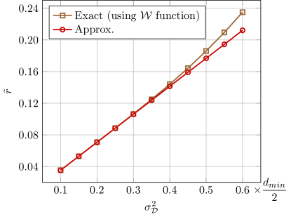
for small Οƒπ’Ÿ2superscriptsubscriptπœŽπ’Ÿ2\sigma_{{\cal D}}^{2} relative to dmin/2subscript𝑑2d_{\min}/2. Fig.Β 5 plots (23) and its approximation (24) as functions of Οƒπ’Ÿ2superscriptsubscriptπœŽπ’Ÿ2\sigma_{{\cal D}}^{2}. Using the approximation for simplicity, r~~π‘Ÿ\tilde{r} then splits the behavior of β„œtrunc​(r)|ΞΈ=Ο€/4evaluated-atsuperscriptβ„œtruncπ‘Ÿπœƒπœ‹4\mathfrak{R}^{\textmd{trunc}}(r)|_{\theta=\pi/4} into two regions, supported by the intervals 𝔯1β‰ˆ{r∈[0,22β€‹Οƒπ’Ÿ2dmin]}subscript𝔯1π‘Ÿ022superscriptsubscriptπœŽπ’Ÿ2subscript𝑑\mathfrak{r}_{1}\approx\{r\in[0,\frac{\sqrt{2}}{2}\frac{\sigma_{{\cal D}}^{2}}{d_{\min}}]\} and 𝔯2β‰ˆ{r∈[22β€‹Οƒπ’Ÿ2dmin,22​dmin]}subscript𝔯2π‘Ÿ22superscriptsubscriptπœŽπ’Ÿ2subscript𝑑22subscript𝑑\mathfrak{r}_{2}\approx\{r\in[\frac{\sqrt{2}}{2}\frac{\sigma_{{\cal D}}^{2}}{d_{\min}},\frac{\sqrt{2}}{2}d_{\min}]\}. This result explains why β„œtrunc​(r,ΞΈ)superscriptβ„œtruncπ‘Ÿπœƒ\mathfrak{R}^{\textmd{trunc}}(r,\theta) in Fig.Β 4 first resembles a circular shape akin to β„œβˆ˜superscriptβ„œ\mathfrak{R}^{\circ} and then inflates along the diagonals deforming into a square-shaped reliability region, β„œβ–‘superscriptβ„œβ–‘\mathfrak{R}^{\Box}, as can be seen when r=0.3​dminπ‘Ÿ0.3subscript𝑑r=0.3d_{\min} in Fig.Β 4 (see the black curve with square-shaped markers). Subsequently, as the magnitude, rπ‘Ÿr, of the perturbation increases and approaches the decision boundaries, β„œtrunc​(r,ΞΈ)superscriptβ„œtruncπ‘Ÿπœƒ\mathfrak{R}^{\text{trunc}}(r,\theta) inflates outwards, resembling pointy leaves that can be modeled as ΞΌ+(1βˆ’ΞΌ)​cos⁑(4​θ+Ο€)πœ‡1πœ‡4πœƒπœ‹\mu+(1-\mu)\cos(4\theta+\pi), where μ∈[1/2,1]>1βˆ’ΞΌ>0πœ‡1211πœ‡0\mu\!\in[1/2,1]\!>\!1-\mu\!>\!0. The analysis also provides restrictions for when square-like reliability regions suggested in the literature (such as [15]) can be justifiable.
Refer to caption
Figure 5: Comparison of r~~π‘Ÿ\tilde{r} in (23) and its approx. in (24) as a function Οƒπ’Ÿ2superscriptsubscriptπœŽπ’Ÿ2\sigma_{{\cal D}}^{2} expressed as a ratio of dmin/2subscript𝑑2d_{\min}/2 (at dmin=1subscript𝑑1d_{\min}=1).

4.3 Dual-stage construction of Ξ©msubscriptΞ©π‘š\Omega_{m}

The reader will notice that our primary objective so far in selecting Ξ©msubscriptΞ©π‘š\Omega_{m} was based on minimizing the probability of incorrect measurements, i.e.,

Ξ©m=arg​maxΞ©~m⁑Pr⁑(Ξ©~mβŠ‚Ξ©T).subscriptΞ©π‘šargsubscriptsubscript~Ξ©π‘šPrsubscript~Ξ©π‘šsubscriptΩ𝑇\displaystyle\Omega_{m}={\hbox{arg}}\max_{\tilde{\Omega}_{m}}\Pr\left(\tilde{\Omega}_{m}\subset\Omega_{T}\right). (25)

This is no doubt a necessary choice to preserve the success of the recovery algorithm as a whole, although we know that a more generic criterion, that is, one that is not at risk of using incorrect observations, would seek the tones with the maximum CNR888In other words, in a generic CS algorithm in which all measurements are 100% reliable, the most effective measurements are the ones which maximize the CNR., i.e., (see (10))

Ξ©msubscriptΞ©π‘š\displaystyle\Omega_{m} =\displaystyle= arg​maxΞ©~mβ‘β€–πšΏΞ©~m​𝒄‖22‖𝓩Ω~mβ€²β€–22=arg​maxΞ©~mβ€‹βˆ‘k∈Ω~m|π’žβ€‹(k)|2|Ξ»βˆ’1​(k)​𝒡​(k)|2.argsubscriptsubscript~Ξ©π‘šsuperscriptsubscriptnormsubscript𝚿subscript~Ξ©π‘šπ’„22superscriptsubscriptnormsubscriptsuperscript𝓩′subscript~Ξ©π‘š22argsubscriptsubscript~Ξ©π‘šsubscriptπ‘˜subscript~Ξ©π‘šsuperscriptπ’žπ‘˜2superscriptsuperscriptπœ†1π‘˜π’΅π‘˜2\displaystyle{\hbox{arg}}\max_{\tilde{\Omega}_{m}}\frac{\|\hbox{\boldmath$\Psi$}_{\tilde{\Omega}_{m}}{\bm{c}}\|_{2}^{2}}{\|\mbox{$\bm{\mathcal{Z}}$}^{\prime}_{\tilde{\Omega}_{m}}\|_{2}^{2}}={\hbox{arg}}\max_{\tilde{\Omega}_{m}}\sum_{k\in\tilde{\Omega}_{m}}\frac{|{\cal C}(k)|^{2}}{|\lambda^{-1}(k){\cal Z}(k)|^{2}}. (26)

Obviously, there is a conflicting interest between (25) and (26), as the former frequently seeks smaller perturbations 𝒳¯^βˆ’βŸ¨π’³Β―^⟩¯^𝒳delimited-⟨⟩¯^𝒳\underline{\hat{{\cal X}}}-\langle\underline{\hat{{\cal X}}}\rangle, since they are the most likely to equal π’Ÿπ’Ÿ{\cal D}, while the latter seeks the largest perturbations to maximize the CNR for enhanced estimation performance.

This prompts us to consider a second recovery stage (i.e., another CS iteration) that uses (26) and produces a new subset of selected tones, denoted by Ξ©mCSsuperscriptsubscriptΞ©π‘šCS\Omega_{m}^{\textmd{CS}}. The second recovery stage takes in Ξ©msubscriptΞ©π‘š\Omega_{m} obtained from (25) and uses it with any of the mentioned CS recovery algorithms to get a CS estimate of π’žπ’ž{\cal C}, denoted by π’žCSsuperscriptπ’žCS{\cal C}^{\textmd{CS}}. This lets us achieve the corrected decoding decision βŸ¨π’³Β―^βˆ’π’žCS⟩delimited-⟨⟩¯^𝒳superscriptπ’žCS\langle\underline{\hat{{\cal X}}}-{\cal C}^{\textmd{CS}}\rangle allowing us to have a higher confidence that π’Ÿ=𝒳¯^βˆ’βŸ¨π’³Β―^βˆ’π’žCSβŸ©π’ŸΒ―^𝒳delimited-⟨⟩¯^𝒳superscriptπ’žCS{\cal D}=\underline{\hat{{\cal X}}}-\langle\underline{\hat{{\cal X}}}\!-{\cal C}^{\textmd{CS}}\rangle compared to the primary assumption that π’Ÿ=𝒳¯^βˆ’βŸ¨π’³Β―^βŸ©π’ŸΒ―^𝒳delimited-⟨⟩¯^𝒳{\cal D}=\underline{\hat{{\cal X}}}-\langle\underline{\hat{{\cal X}}}\rangle. This is because the decoding error in βŸ¨π’³Β―^⟩=βŸ¨π’³+π’ŸβŸ©=βŸ¨π’³+π’ž+Ξ»βˆ’1β€‹π’΅βŸ©delimited-⟨⟩¯^𝒳delimited-βŸ¨βŸ©π’³π’Ÿdelimited-βŸ¨βŸ©π’³π’žsuperscriptπœ†1𝒡\langle\underline{\hat{{\cal X}}}\rangle=\langle{\cal X}+\mathcal{D}\rangle=\langle{\cal X}+{\cal C}+\lambda^{-1}{\cal Z}\rangle depends on the value of π’žπ’ž{\cal C}, whereas the error in βŸ¨π“§Β―^βˆ’π’žCS⟩=βŸ¨π’³+Ξ”βŸ©=βŸ¨π’³+β„°CS+Ξ»βˆ’1β€‹π’΅βŸ©delimited-⟨⟩¯^𝓧superscriptπ’žCSdelimited-βŸ¨βŸ©π’³Ξ”delimited-βŸ¨βŸ©π’³superscriptβ„°CSsuperscriptπœ†1𝒡\langle\underline{\hat{\mbox{$\bm{\mathcal{X}}$}}}-{\cal C}^{\textmd{CS}}\rangle=\langle{\cal X}+\Delta\rangle=\langle{\cal X}+{\cal E}^{\textmd{CS}}+\lambda^{-1}{\cal Z}\rangle depends on the estimation error β„°CS=π’žβˆ’π’žCSsuperscriptβ„°CSπ’žsuperscriptπ’žCS{\cal E}^{\textmd{CS}}={\cal C}-{\cal C}^{\textmd{CS}} of π’žπ’ž{\cal C} which is expected to be smaller than π’žπ’ž{\cal C} itself. These results follow from (3) and (12).

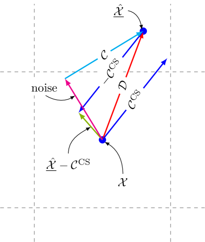
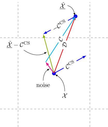
As illustrated in Figs.Β 6 and 7, it is possible now to use these carriers that have the largest values of the perturbations, 𝒳¯^βˆ’βŸ¨π’³Β―^βˆ’π’žCS⟩¯^𝒳delimited-⟨⟩¯^𝒳superscriptπ’žCS\underline{\hat{{\cal X}}}-\langle\underline{\hat{{\cal X}}}-{\cal C}^{\textmd{CS}}\rangle (or even the carriers with the largest values of π’žCSsuperscriptπ’žCS{\cal C}^{\textmd{CS}}), as the new CS measurements, without worrying much about how close 𝒳¯^Β―^𝒳\underline{\hat{{\cal X}}} is to the decision boundaries. Note, however, that we never have access to π’žπ’ž{\cal C}, 𝒡𝒡{\cal Z}, or β„°CSsuperscriptβ„°CS{\cal E}^{\textmd{CS}}, and therefore we can rely only on observable variables, such as π’Ÿπ’Ÿ{\cal D} and ΔΔ\Delta, to practically maximize the CNR. More importantly, these variables themselves are not always obtainable, since it is not necessarily the case that π’Ÿ=𝒳¯^βˆ’βŸ¨π’³Β―^βˆ’π’žCSβŸ©π’ŸΒ―^𝒳delimited-⟨⟩¯^𝒳superscriptπ’žCS{\cal D}=\underline{\hat{{\cal X}}}-\langle\underline{\hat{{\cal X}}}-{\cal C}^{\textmd{CS}}\rangle or that Ξ”=𝒳¯^βˆ’π’žCSβˆ’βŸ¨π’³Β―^βˆ’π’žCSβŸ©Ξ”Β―^𝒳superscriptπ’žCSdelimited-⟨⟩¯^𝒳superscriptπ’žCS\Delta=\underline{\hat{{\cal X}}}-{\cal C}^{\textmd{CS}}-\langle\underline{\hat{{\cal X}}}-{\cal C}^{\textmd{CS}}\rangle (which is the main reason that we repeat CS over a subset of measurements). Instead, we have to rely on the observable variables, 𝒳¯^βˆ’βŸ¨π’³Β―^βˆ’π’žCS⟩¯^𝒳delimited-⟨⟩¯^𝒳superscriptπ’žCS\underline{\hat{{\cal X}}}-\langle\underline{\hat{{\cal X}}}-{\cal C}^{\textmd{CS}}\rangle and π’žCSsuperscriptπ’žCS{\cal C}^{\textmd{CS}}, for this task. The availability of these two observable variables grants us the flexibility of computing CNR in two different ways, both of which are suitable for different scenarios. The first is suited for a high SNR and low CS estimation quality (see Fig.Β 6), while the second is suited for a low SNR and high CS estimation quality (see Fig.Β 7). Dropping the coefficient index, kπ‘˜k, these are:

  1. 1.

    High SNR, large β„°c​ssuperscriptℰ𝑐𝑠{\cal E}^{cs}:

    CNR^Ξ»superscript^CNRπœ†\displaystyle\widehat{\textmd{CNR}}^{\lambda} =\displaystyle= |𝒳¯^βˆ’βŸ¨π’³Β―^βˆ’π’žCS⟩|2|𝒳¯^βˆ’π’žCSβˆ’βŸ¨π’³Β―^βˆ’π’žCS⟩|2superscriptΒ―^𝒳delimited-⟨⟩¯^𝒳superscriptπ’žCS2superscriptΒ―^𝒳superscriptπ’žCSdelimited-⟨⟩¯^𝒳superscriptπ’žCS2\displaystyle\frac{|\,\underline{\hat{{\cal X}}}-\langle\underline{\hat{{\cal X}}}-{\cal C}^{\textmd{CS}}\rangle|^{2}}{|\,\underline{\hat{{\cal X}}}-{\cal C}^{\textmd{CS}}-\langle\underline{\hat{{\cal X}}}-{\cal C}^{\textmd{CS}}\rangle|^{2}}
    =\displaystyle= |π’Ÿ|2|Ξ”|2,iffβ€‹βŸ¨π“§Β―^βˆ’π’žCS⟩=𝒳superscriptπ’Ÿ2superscriptΞ”2iffdelimited-⟨⟩¯^𝓧superscriptπ’žCS𝒳\displaystyle\frac{|\mathcal{D}|^{2}}{|\Delta|^{2}},\quad\textmd{iff}\>\>\langle\underline{\hat{\mbox{$\bm{\mathcal{X}}$}}}-{\cal C}^{\textmd{CS}}\rangle={\cal X}
    =\displaystyle= |π’ž+Ξ»βˆ’1​𝒡|2|β„°CS+Ξ»βˆ’1​𝒡|2β‰Ξ»βˆ’1β†’0|π’ž|2|β„°CS|2superscriptπ’žsuperscriptπœ†1𝒡2superscriptsuperscriptβ„°CSsuperscriptπœ†1𝒡2β†’superscriptπœ†10asymptotically-equalssuperscriptπ’ž2superscriptsuperscriptβ„°CS2\displaystyle\frac{|{\cal C}+\lambda^{-1}{\cal Z}|^{2}}{|{\cal E}^{\textmd{CS}}+\lambda^{-1}{\cal Z}|^{2}}\quad\underset{\lambda^{-1}\rightarrow 0}{\asymp}\quad\frac{|{\cal C}|^{2}}{|{\cal E}^{\textmd{CS}}|^{2}}

    where the symbol ≍asymptotically-equals\asymp means that the expression on the left hand side of this symbol is asymptotically equal to the expression on the right hand side.
    Refer to caption
    Figure 6: Computing CNR for the case of high SNR and low CS estimation quality
  2. 2.

    Low SNR, small β„°c​ssuperscriptℰ𝑐𝑠{\cal E}^{cs}:

    CNR^β„°CSsuperscript^CNRsuperscriptβ„°CS\displaystyle\widehat{\textmd{CNR}}^{{\cal E}^{\textmd{CS}}} =\displaystyle= |π’žCS|2|𝒳¯^βˆ’π’žCSβˆ’βŸ¨π’³Β―^βˆ’π’žCS⟩|2superscriptsuperscriptπ’žCS2superscript^¯𝒳superscriptπ’žCSdelimited-⟨⟩¯^𝒳superscriptπ’žCS2\displaystyle\frac{|\,{\cal C}^{\textmd{CS}}|^{2}}{|\,\hat{\underline{{\cal X}}}-{\cal C}^{\textmd{CS}}-\langle\underline{\hat{{\cal X}}}-{\cal C}^{\textmd{CS}}\rangle|^{2}}
    =\displaystyle= |π’žCS|2|Ξ”|2,iffβ€‹βŸ¨π’³Β―^βˆ’π’žCS⟩=𝒳superscriptsuperscriptπ’žCS2superscriptΞ”2iffdelimited-⟨⟩¯^𝒳superscriptπ’žCS𝒳\displaystyle\frac{|{\cal C}^{\textmd{CS}}|^{2}}{|\Delta|^{2}},\quad\textmd{iff}\>\>\langle\underline{\hat{{\cal X}}}-{\cal C}^{\textmd{CS}}\rangle={\cal X}
    =\displaystyle= |π’ž+β„°CS|2|Ξ»βˆ’1​𝒡+β„°CS|2≍ℰCSβ†’0|π’ž|2|Ξ»βˆ’1​𝒡|2.superscriptπ’žsuperscriptβ„°CS2superscriptsuperscriptπœ†1𝒡superscriptβ„°CS2β†’superscriptβ„°CS0asymptotically-equalssuperscriptπ’ž2superscriptsuperscriptπœ†1𝒡2\displaystyle\frac{|{\cal C}+{\cal E}^{\textmd{CS}}|^{2}}{|\lambda^{-1}{\cal Z}+{\cal E}^{\textmd{CS}}|^{2}}\quad\underset{{\cal E}^{\textmd{CS}}\rightarrow 0}{\asymp}\quad\frac{|{\cal C}|^{2}}{|\lambda^{-1}{\cal Z}|^{2}}.
    Refer to caption
    Figure 7: Computing CNR for the case of low SNR and high CS estimation quality

Although the second ratio CNR^β„°CSsuperscript^CNRsuperscriptβ„°CS\widehat{\textmd{CNR}}^{{\cal E}^{\textmd{CS}}} more vividly resembles the CNR defined in (26), the first ratio is more effective in this work as the inherent complexity of CS based methods justifies itself in severe clipping scenarios and hence expectedly higher CS error (i.e., large β„°CSsuperscriptβ„°CS{\cal E}^{\textmd{CS}}). Consequently, we select the differential measurements corresponding to the maximum |Ξ©mCS|superscriptsubscriptΞ©π‘šCS|\Omega_{m}^{\textmd{CS}}| ratios999Obviously, the number of tones |Ξ©mCS|superscriptsubscriptΞ©π‘šCS|\Omega_{m}^{\textmd{CS}}| need not be equivalent to the original number |Ξ©m|subscriptΞ©π‘š|\Omega_{m}|, and a wealth of possibilities emerges in relating these two parameters for optimal performance.,

Ξ©mCS=arg​{CNR^iΞ»}i=Nβˆ’|Ξ©mCS|+1N,superscriptsubscriptΞ©π‘šCSargsuperscriptsubscriptsubscriptsuperscript^CNRπœ†π‘–π‘–π‘superscriptsubscriptΞ©π‘šCS1𝑁\displaystyle\Omega_{m}^{\textmd{CS}}={\hbox{arg}}\left\{\widehat{\textmd{{CNR}}}^{\lambda}_{i}\right\}_{i=N-|\Omega_{m}^{\textmd{CS}}|+1}^{N}, (29)

and the new CS model is

𝓨ΩmCSβ€²subscriptsuperscript𝓨′superscriptsubscriptΞ©π‘šCS\displaystyle\mbox{$\bm{\mathcal{Y}}$}^{\prime}_{\Omega_{m}^{\textmd{CS}}} =\displaystyle= 𝐒ΩmCS​(𝓧¯^βˆ’βŸ¨π“§Β―^βˆ’π“’CS⟩)+𝓩ΩmCSβ€²subscript𝐒superscriptsubscriptΞ©π‘šCSΒ―^𝓧delimited-⟨⟩¯^𝓧superscript𝓒CSsuperscriptsubscript𝓩superscriptsubscriptΞ©π‘šCSβ€²\displaystyle{\bf S}_{\Omega_{m}^{\textmd{CS}}}(\underline{\hat{\mbox{$\bm{\mathcal{X}}$}}}-\langle\underline{\hat{\mbox{$\bm{\mathcal{X}}$}}}-\mbox{$\bm{\mathcal{C}}$}^{\textmd{CS}}\rangle)+\mbox{$\bm{\mathcal{Z}}$}_{\Omega_{m}^{\textmd{CS}}}^{\prime} (30)
=\displaystyle= 𝚿ΩmCS​𝒄+𝓩ΩmCSβ€²,subscript𝚿superscriptsubscriptΞ©π‘šCS𝒄superscriptsubscript𝓩superscriptsubscriptΞ©π‘šCSβ€²\displaystyle\hbox{\boldmath$\Psi$}_{\Omega_{m}^{\textmd{CS}}}{\bm{c}}+\mbox{$\bm{\mathcal{Z}}$}_{\Omega_{m}^{\textmd{CS}}}^{\prime},

which produces an improved estimate, 𝓒revsuperscript𝓒rev\mbox{$\bm{\mathcal{C}}$}^{\textmd{rev}}. This new estimate of the clipping distortion from a different subset of reliable and stronger measurements can then be subtracted from 𝓧¯^Β―^𝓧\underline{\hat{\mbox{$\bm{\mathcal{X}}$}}}, and a revised set of decoding decisions, βŸ¨π“§Β―^βˆ’π“’rev⟩delimited-⟨⟩¯^𝓧superscript𝓒rev\langle\underline{\hat{\mbox{$\bm{\mathcal{X}}$}}}-\mbox{$\bm{\mathcal{C}}$}^{\textmd{rev}}\rangle, can be made.

4.4 On selecting the cardinality |Ξ©m|subscriptΞ©π‘š|\Omega_{m}|
Refer to caption
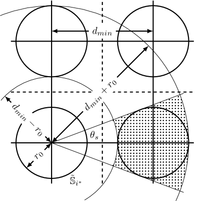
Figure 8: Illustrating how the integral over the shaded region upper-bounds the integral over π•Š~isubscript~π•Šπ‘–\tilde{\mathbb{S}}_{i}.

In the method we proposed, it is assumed throughout the above discussion that the observations supplied to the CS algorithm were true measurements of the actual perturbations caused by clipping and additive noise. Although this is a mild restriction in practice, a guarantee must nonetheless be established that any selected Ξ©msubscriptΞ©π‘š\Omega_{m} and |Ξ©m|subscriptΞ©π‘š|\Omega_{m}| according to Section 4 will not result in CS failure. This requires that the number of measurements |Ξ©m|subscriptΞ©π‘š|\Omega_{m}| be both small enough to minimize the probability of incorrect measurements, and also large enough relative to the sparsity level of 𝒄𝒄{\bm{c}} to ensure meeting recovery bounds of CS.

To this end, we derive a simple lower bound on the probability of Ξ©mβŠ‚Ξ©TsubscriptΞ©π‘šsubscriptΩ𝑇\Omega_{m}\!\subset\!\Omega_{T} by deriving a lower bound on the probability that π’Ÿπ’Ÿ{\cal D} is indeed equal to 𝒳¯^βˆ’βŸ¨π’³Β―^⟩¯^𝒳delimited-⟨⟩¯^𝒳\underline{\hat{{\cal X}}}-\langle\underline{\hat{{\cal X}}}\rangle. We study this for two cases: when 𝒳¯^βˆ’βŸ¨π’³Β―^⟩¯^𝒳delimited-⟨⟩¯^𝒳\underline{\hat{{\cal X}}}-\langle\underline{\hat{{\cal X}}}\rangle is observed within a disk of radius rosubscriptπ‘Ÿπ‘œr_{o} from βŸ¨π’³Β―^⟩delimited-⟨⟩^¯𝒳\langle\hat{\underline{\mathcal{X}}}\rangle, i.e., Ξ©m={k∈Ω:|𝒳¯^​(k)βˆ’βŸ¨π’³Β―^​(k)⟩|<ro}subscriptΞ©π‘šconditional-setπ‘˜Ξ©Β―^π’³π‘˜delimited-⟨⟩¯^π’³π‘˜subscriptπ‘Ÿπ‘œ\Omega_{m}\!=\!\{k\!\in\!\Omega\!:\!|\underline{\hat{{\cal X}}}(k)\!-\!\langle\underline{\hat{{\cal X}}}(k)\rangle|\!<\!r_{o}\}, and when it is observed within a square of side length 2​ro2subscriptπ‘Ÿπ‘œ2r_{o} centered at the QAM symbols 𝓐𝓐\bm{\mathcal{A}}. We focus on the first case since it is more difficult to estimate, and directly give the result of the second since it is comparably straightforward. To this end, define a safe region, π•Š~i={π’œi+π’°βˆˆβ„‚:|𝒰|<ro}subscript~π•Šπ‘–conditional-setsubscriptπ’œπ‘–π’°β„‚π’°subscriptπ‘Ÿπ‘œ\tilde{\mathbb{S}}_{i}=\{{\cal A}_{i}+{\cal U}\in\mathbb{C}:|{\cal U}|<r_{o}\}, for decoding 𝒳¯^​(k)Β―^π’³π‘˜\underline{\hat{{\cal X}}}(k) within its square ML decision region, β„šisubscriptβ„šπ‘–\mathbb{Q}_{i}, and denote the collection of all these safe regions by π•Š=⋃i=0Mβˆ’1π•Š~iπ•Šsuperscriptsubscript𝑖0𝑀1subscript~π•Šπ‘–\mathbb{S}\!=\!\bigcup_{i=0}^{M-1}\tilde{\mathbb{S}}_{i}. Our objective is to select |Ξ©m|subscriptΞ©π‘š|\Omega_{m}| such that Pr⁑(Ξ©mβŠ‚Ξ©T∣|Ξ©m|)PrsubscriptΞ©π‘šsubscriptΩ𝑇subscriptΞ©π‘š\Pr\left(\Omega_{m}\subset\Omega_{T}\big{|}|\Omega_{m}|\right) is high given a minimum amount of required measurement for CS success.

Dropping the tone index, this will require finding Pr⁑(π’Ÿβˆˆπ•Š)Prπ’Ÿπ•Š\Pr({\cal D}\in\mathbb{S}), which requires evaluating an integral of fπ’Ÿsubscriptπ‘“π’Ÿf_{{\cal D}} over (non-centered) discrete disks in the complex plane (see Fig.Β 8). Since this is difficult, we will use an upper bound based on evaluating fπ’Ÿsubscriptπ‘“π’Ÿf_{{\cal D}} over centered disks that cover these regions and then slice out the irrelevant regions. More specifically, the integral βˆ«π’Ÿβˆˆπ•Š~isubscriptπ’Ÿsubscript~π•Šπ‘–\int_{{\cal D}\in\tilde{\mathbb{S}}_{i}} over the disk π•Š~isubscript~π•Šπ‘–\tilde{\mathbb{S}}_{i} of a nearest neighbor will be bounded by the integral over the area highlighted by the shaded region in Fig.Β 8. This region covers the difference between the outer and inner sectors defined by radii dmin+rosubscript𝑑subscriptπ‘Ÿπ‘œd_{\min}+r_{o} and dminβˆ’rosubscript𝑑subscriptπ‘Ÿπ‘œd_{\min}-r_{o}, respectively, and a common angle, ΞΈs=2​sinβˆ’1⁑(rodmin)subscriptπœƒπ‘ 2superscript1subscriptπ‘Ÿπ‘œsubscript𝑑\theta_{s}=2\sin^{-1}\left(\frac{r_{o}}{d_{\min}}\right). In effect, the area of π•Š~isubscript~π•Šπ‘–\tilde{\mathbb{S}}_{i} is strictly less than ΞΈs2​π​[π​(dmin+ro)2βˆ’Ο€β€‹(dminβˆ’ro)2]subscriptπœƒπ‘ 2πœ‹delimited-[]πœ‹superscriptsubscript𝑑subscriptπ‘Ÿπ‘œ2πœ‹superscriptsubscript𝑑subscriptπ‘Ÿπ‘œ2\frac{\theta_{s}}{2\pi}[\pi(d_{\min}+r_{o})^{2}-\pi(d_{\min}-r_{o})^{2}] and therefore Pr⁑(π’Ÿβˆˆπ•Š~i)<ΞΈs2​π​(Fπ’Ÿβ€‹(dmin+ro)βˆ’Fπ’Ÿβ€‹(dminβˆ’ro))Prπ’Ÿsubscript~π•Šπ‘–subscriptπœƒπ‘ 2πœ‹subscriptπΉπ’Ÿsubscript𝑑subscriptπ‘Ÿπ‘œsubscriptπΉπ’Ÿsubscript𝑑subscriptπ‘Ÿπ‘œ\Pr({\cal D}\in\tilde{\mathbb{S}}_{i})<\frac{\theta_{s}}{2\pi}\left(F_{{\cal D}}(d_{\min}+r_{o})-F_{{\cal D}}(d_{\min}-r_{o})\right) for the nearest neighbor. Consequently,

Pr⁑(Ξ©mβŠ‚Ξ©T∣|Ξ©m|)PrsubscriptΞ©π‘šsubscriptΩ𝑇subscriptΞ©π‘š\displaystyle\Pr(\Omega_{m}\!\!\subset\!\Omega_{T}\big{|}|\Omega_{m}|)\!\!\!\! =\displaystyle= Pr⁑(β‹‚i=1|Ξ©m|Ξ©m​(i)∈ΩT)Prsuperscriptsubscript𝑖1subscriptΞ©π‘šsubscriptΞ©π‘šπ‘–subscriptΩ𝑇\displaystyle\!\!\!\!\Pr\left(\bigcap_{i=1}^{|\Omega_{m}|}\Omega_{m}(i)\in\Omega_{T}\right)
=\displaystyle= Pr(βŸ¨π’³Β―^⟩=𝒳||𝒳¯^βˆ’βŸ¨π’³Β―^⟩|<ro)|Ξ©m|=Pr(π’Ÿ=𝒳¯^βˆ’βŸ¨π’³Β―^⟩|π’Ÿβˆˆπ•Š)|Ξ©m|\displaystyle\!\!\!\!\Pr\left(\langle\underline{\hat{{\cal X}}}\rangle={\cal X}\,\big{|}|\,\underline{\hat{{\cal X}}}\!-\!\langle\underline{\hat{{\cal X}}}\rangle|\!<r_{o}\right)^{|\Omega_{m}|}=\Pr({\cal D}=\underline{\hat{{\cal X}}}-\langle\underline{\hat{{\cal X}}}\rangle\big{|}{\cal D}\in\mathbb{S})^{|\Omega_{m}|}
=\displaystyle= (Pr⁑(|π’Ÿ|<ro,π’Ÿβˆˆπ•Š)Pr⁑(π’Ÿβˆˆπ•Š))|Ξ©m|=(Pr⁑(|π’Ÿ|<ro)Pr⁑(π’Ÿβˆˆπ•Š))|Ξ©m|superscriptPrπ’Ÿsubscriptπ‘Ÿπ‘œπ’Ÿπ•ŠPrπ’Ÿπ•ŠsubscriptΞ©π‘šsuperscriptPrπ’Ÿsubscriptπ‘Ÿπ‘œPrπ’Ÿπ•ŠsubscriptΞ©π‘š\displaystyle\!\!\!\!\left(\frac{\Pr(|{\cal D}|<r_{o},{\cal D}\in\mathbb{S})}{\Pr({\cal D}\in\mathbb{S})}\right)^{|\Omega_{m}|}=\left(\frac{\Pr(|{\cal D}|<r_{o})}{\Pr({\cal D}\in\mathbb{S})}\right)^{|\Omega_{m}|}
>\displaystyle> 𝔽|π’Ÿ||Ξ©m|​(ro)/(𝔽|π’Ÿ|​(ro)+8π​sinβˆ’1⁑rodmin​[𝔽|π’Ÿ|​(dmin+ro)βˆ’π”½|π’Ÿ|​(dminβˆ’ro)])|Ξ©m|subscriptsuperscript𝔽subscriptΞ©π‘šπ’Ÿsubscriptπ‘Ÿπ‘œsuperscriptsubscriptπ”½π’Ÿsubscriptπ‘Ÿπ‘œ8πœ‹superscript1subscriptπ‘Ÿπ‘œsubscript𝑑delimited-[]subscriptπ”½π’Ÿsubscript𝑑subscriptπ‘Ÿπ‘œsubscriptπ”½π’Ÿsubscript𝑑subscriptπ‘Ÿπ‘œsubscriptΞ©π‘š\displaystyle\!\!\!\!\mathbb{F}^{|\Omega_{m}|}_{|{\cal D}|}(r_{o})/\Big{(}\mathbb{F}_{|{\cal D}|}(r_{o})+\frac{8}{\pi}\sin^{-1}\!\frac{r_{o}}{d_{\min}}\left[\mathbb{F}_{|{\cal D}|}(d_{\min}\!+\!r_{o})\!-\!\mathbb{F}_{|{\cal D}|}(d_{\min}\!-\!r_{o})\right]\!\Big{)}^{\!|\Omega_{m}|}
>\displaystyle> (1βˆ’eβˆ’ro22β€‹Οƒπ’Ÿ2)|Ξ©m|/(1βˆ’eβˆ’ro22β€‹Οƒπ’Ÿ2+8π​sinβˆ’1⁑rodmin​sinh⁑(ro​dminΟƒπ’Ÿ2)​eβˆ’(dmin2+ro2)2β€‹Οƒπ’Ÿ2)|Ξ©m|.superscript1superscript𝑒superscriptsubscriptπ‘Ÿπ‘œ22superscriptsubscriptπœŽπ’Ÿ2subscriptΞ©π‘šsuperscript1superscript𝑒superscriptsubscriptπ‘Ÿπ‘œ22superscriptsubscriptπœŽπ’Ÿ28πœ‹superscript1subscriptπ‘Ÿπ‘œsubscript𝑑subscriptπ‘Ÿπ‘œsubscript𝑑superscriptsubscriptπœŽπ’Ÿ2superscript𝑒superscriptsubscript𝑑2superscriptsubscriptπ‘Ÿπ‘œ22superscriptsubscriptπœŽπ’Ÿ2subscriptΞ©π‘š\displaystyle\!\!\!\big{(}1-e^{\frac{-r_{o}^{2}}{2\sigma_{{\cal D}}^{2}}}\big{)}^{|\Omega_{m}|}/\Big{(}1-e^{\frac{-r_{o}^{2}}{2\sigma_{{\cal D}}^{2}}}\!+\!\frac{8}{\pi}\sin^{-1}\!\!\frac{r_{o}}{d_{\min}}\sinh\!\Big{(}\frac{r_{o}d_{\min}}{\sigma_{{\cal D}}^{2}}\Big{)}e^{\frac{-(d_{\min}^{2}+r_{o}^{2})}{2\sigma_{{\cal D}}^{2}}}\!\!\Big{)}^{|\Omega_{m}|}. (32)

In the case where the average distortion is large and square regions π•Šβ–‘=⋃i=0Mβˆ’1π•Š~iβ–‘superscriptπ•Šβ–‘superscriptsubscript𝑖0𝑀1subscriptsuperscript~π•Šβ–‘π‘–\mathbb{S}^{\Box}\!=\!\bigcup_{i=0}^{M-1}\tilde{\mathbb{S}}^{\Box}_{i} of side-length 2​ro2subscriptπ‘Ÿπ‘œ2r_{o} are used, pursuing the same logic above we just replace the ratio in (4.4) with

Pr⁑(π’Ÿβˆˆπ•Š~iβˆ—β–‘)Pr⁑(π’Ÿβˆˆπ•Šβ–‘)β‰ˆ[1βˆ’2​Q​(roΟƒπ’Ÿ)]2[1βˆ’2​Q​(roΟƒπ’Ÿ)]2+4​[Q​(dminβˆ’roΟƒπ’Ÿ)βˆ’Q​(dmin+roΟƒπ’Ÿ)]2Prπ’Ÿsubscriptsuperscript~π•Šβ–‘superscript𝑖Prπ’Ÿsuperscriptπ•Šβ–‘superscriptdelimited-[]12𝑄subscriptπ‘Ÿπ‘œsubscriptπœŽπ’Ÿ2superscriptdelimited-[]12𝑄subscriptπ‘Ÿπ‘œsubscriptπœŽπ’Ÿ24superscriptdelimited-[]𝑄subscript𝑑subscriptπ‘Ÿπ‘œsubscriptπœŽπ’Ÿπ‘„subscript𝑑subscriptπ‘Ÿπ‘œsubscriptπœŽπ’Ÿ2\displaystyle\frac{\Pr({\cal D}\in{\tilde{\mathbb{S}}}^{\Box}_{i^{*}})}{\Pr({\cal D}\in\mathbb{S}^{\Box})}\approx\frac{\left[1-2Q(\frac{r_{o}}{\sigma_{{\cal D}}})\right]^{2}}{\left[1-2Q(\frac{r_{o}}{\sigma_{{\cal D}}})\right]^{2}\!+\!4\left[Q(\frac{d_{\min}-r_{o}}{\sigma_{{\cal D}}})-Q(\frac{d_{\min}+r_{o}}{\sigma_{{\cal D}}})\right]^{2}} (33)

and raise it to the power |Ξ©m|subscriptΞ©π‘š|\Omega_{m}| to obtain Pr⁑(Ξ©mβŠ‚Ξ©T∣|Ξ©m|)PrsubscriptΞ©π‘šsubscriptΩ𝑇subscriptΞ©π‘š\Pr(\Omega_{m}\!\!\subset\!\Omega_{T}\big{|}|\Omega_{m}|), where Q𝑄Q is the familiar tail probability function. The user must then choose |Ξ©mΟ„|=arg​max|Ξ©m|⁑[Pr⁑(Ξ©mβŠ‚Ξ©T∣|Ξ©m|)>Ο„]superscriptsubscriptΞ©π‘šπœargsubscriptsubscriptΞ©π‘šPrsubscriptΞ©π‘šsubscriptΩ𝑇subscriptΞ©π‘šπœ|\Omega_{m}^{\,\tau}|={\hbox{arg}}\max_{|\Omega_{m}|}[\Pr(\Omega_{m}\subset\Omega_{T}\big{|}|\Omega_{m}|)>\tau] where Ο„πœ\tau is selected so as to supply as much information to the CS algorithm as possible while remaining in a safe region of correct measurements. Furthermore, given a clipping threshold, γ𝛾\gamma, we have an expected sparsity level, 𝔼​[|ℐ𝒄|]𝔼delimited-[]subscriptℐ𝒄\mathbb{E}[|{\cal I}_{{\bm{c}}}|], and variance Οƒ|ℐ𝒄|2superscriptsubscript𝜎subscriptℐ𝒄2\sigma_{|\mathcal{I}_{{\bm{c}}}|}^{2}, which need to be taken into account when using sparse recovery techniques [8]. We will denote this minimum required number of frequency observations to recover an |ℐ𝒄|subscriptℐ𝒄|{\cal I}_{{\bm{c}}}|-sparse vector in time by |Ξ©mΞ³|superscriptsubscriptΞ©π‘šπ›Ύ|\Omega_{m}^{\gamma}| to stress its strong dependence on γ𝛾\gamma, and take |Ξ©m|=max⁑(|Ξ©mΟ„|,|Ξ©mΞ³|)subscriptΞ©π‘šsuperscriptsubscriptΞ©π‘šπœsuperscriptsubscriptΞ©π‘šπ›Ύ|\Omega_{m}|=\max(|\Omega_{m}^{\tau}|,|\Omega_{m}^{\gamma}|). The same can be done with the optional second stage |Ξ©mCS|superscriptsubscriptΞ©π‘šCS|\Omega_{m}^{\textmd{CS}}|.

Suppose however, after taking all the protective measures thus far, that an incorrect measurement was nonetheless supplied to the CS algorithm. Does this result in CS failure? Luckily, in this application the answer is no. Recall first the decoding-error vector π“”β‰œπ“§βˆ’βŸ¨π“§Β―^βŸ©β‰œπ“”π“§delimited-⟨⟩¯^𝓧\mbox{$\bm{\mathcal{E}}$}\triangleq\mbox{$\bm{\mathcal{X}}$}-\langle\underline{\hat{\mbox{$\bm{\mathcal{X}}$}}}\rangle used to motivate (9). When a decoding error is made at the kπ‘˜kth coefficient, an incorrect measurement 𝒳¯^​(k)βˆ’βŸ¨π’³Β―^​(k)⟩=𝒳​(k)+π’Ÿβ€‹(k)βˆ’βŸ¨π’³Β―^​(k)βŸ©β‰œπ’Ÿβ€‹(k)+ℰ​(k)Β―^π’³π‘˜delimited-⟨⟩¯^π’³π‘˜π’³π‘˜π’Ÿπ‘˜delimited-⟨⟩¯^π’³π‘˜β‰œπ’Ÿπ‘˜β„°π‘˜\underline{\hat{{\cal X}}}(k)-\langle\underline{\hat{{\cal X}}}(k)\rangle={\cal X}(k)+{\cal D}(k)-\langle\underline{\hat{{\cal X}}}(k)\rangle\triangleq{\cal D}(k)+{\cal E}(k) is supplied and it follows from (9) that the incorrect measurement has no impact on the performance of CS. Note that the nonzero entries of 𝓔𝓔\bm{\mathcal{E}} are quantized and bounded since 𝓧𝓧\bm{\mathcal{X}} and βŸ¨π“§Β―^βŸ©βˆˆπ“Ndelimited-⟨⟩¯^𝓧superscript𝓐𝑁\langle\underline{\hat{\mbox{$\bm{\mathcal{X}}$}}}\rangle\in\mbox{$\bm{\mathcal{A}}$}^{N}. Furthermore, assuming most equalized coefficients 𝒳¯^​(k)Β―^π’³π‘˜\underline{\hat{{\cal X}}}(k) are decoded correctly, 𝓔𝓔\bm{\mathcal{E}} is also sparse.

The general differential model (i.e., the one that is not confined to the carriers in Ξ©msubscriptΞ©π‘š\Omega_{m}) becomes

𝓧¯^βˆ’βŸ¨π“§Β―^⟩=𝓒+πš²βˆ’1​𝓩+𝓔¯^𝓧delimited-⟨⟩¯^𝓧𝓒superscript𝚲1𝓩𝓔\displaystyle\underline{\hat{\mbox{$\bm{\mathcal{X}}$}}}-\langle\underline{\hat{\mbox{$\bm{\mathcal{X}}$}}}\rangle=\mbox{$\bm{\mathcal{C}}$}+\hbox{\boldmath$\Lambda$}^{-1}\mbox{$\bm{\mathcal{Z}}$}+\mbox{$\bm{\mathcal{E}}$} (34)

The first term added to 𝓒𝓒\bm{\mathcal{C}} is the (dense) Gaussian noise vector, while the second is a structured-noise term. Equation (34) matches the model in [16], and it is demonstrated therein how it is possible to recover 𝓒𝓒\bm{\mathcal{C}} from such noise via variations in the CS algorithm. The main results of the paper are summarized in the algorithm listed in Table 1.

parameters: N𝑁N, M𝑀M, γ𝛾\gamma, ΞΌπœ‡\mu, Ο„πœ\tau, Οƒz2superscriptsubscriptπœŽπ‘§2\sigma_{z}^{2}, Ο΅italic-Ο΅\epsilon
input: 𝓨𝓨\bm{\mathcal{Y}}, 𝚲𝚲\Lambda,
output: 𝓧^=βŸ¨π“§Β―^βˆ’π“’CS⟩^𝓧delimited-⟨⟩¯^𝓧superscript𝓒CS\hat{\mbox{$\bm{\mathcal{X}}$}}=\langle\underline{\hat{\mbox{$\bm{\mathcal{X}}$}}}-\mbox{$\bm{\mathcal{C}}$}^{\textmd{CS}}\rangle
1. Compute 𝓧¯^Β―^𝓧\underline{\hat{\mbox{$\bm{\mathcal{X}}$}}}, βŸ¨π“§Β―^⟩delimited-⟨⟩¯^𝓧\langle\underline{\hat{\mbox{$\bm{\mathcal{X}}$}}}\rangle, |𝓧¯^βˆ’βŸ¨π“§Β―^⟩|Β―^𝓧delimited-⟨⟩¯^𝓧|\underline{\hat{\mbox{$\bm{\mathcal{X}}$}}}-\langle\underline{\hat{\mbox{$\bm{\mathcal{X}}$}}}\rangle|, θ𝓧¯^βˆ’βŸ¨π“§Β―^⟩subscriptπœƒΒ―^𝓧delimited-⟨⟩¯^𝓧\theta_{\underline{\hat{\bm{{\cal X}}}}-\langle\underline{\hat{\bm{{\cal X}}}}\rangle}, σ𝓓2superscriptsubscriptπœŽπ““2\sigma_{\bm{{\cal D}}}^{2}, |Ξ©mΟ„|superscriptsubscriptΞ©π‘šπœ|\Omega_{m}^{\tau}|, |Ξ©mΞ³|superscriptsubscriptΞ©π‘šπ›Ύ|\Omega_{m}^{\gamma}|
2. Case: Severe clipping, for k=1,…,Nπ‘˜1…𝑁k=1,\ldots,N
β„œβ€‹(k)β†’(β​(Ξ±cos⁑θ+Ξ±sin⁑θ+β​αcos⁑θ+sin⁑θ))βˆ’1β†’β„œπ‘˜superscript𝛽superscriptπ›Όπœƒsuperscriptπ›Όπœƒπ›½superscriptπ›Όπœƒπœƒ1\mathfrak{R}(k)\rightarrow\left(\beta(\alpha^{\cos\theta}+\alpha^{\sin\theta}+\beta\alpha^{\cos\theta+\sin\theta})\right)^{-1}; Ξ±=e2​dmin​rΟƒπ’Ÿβ€‹(k)2𝛼superscript𝑒2subscriptπ‘‘π‘ŸsuperscriptsubscriptπœŽπ’Ÿπ‘˜2\alpha=e^{\frac{2d_{\min}r}{\sigma_{{\cal D}(k)}^{2}}}, Ξ²=eβˆ’dminΟƒπ’Ÿβ€‹(k)2𝛽superscript𝑒subscript𝑑superscriptsubscriptπœŽπ’Ÿπ‘˜2\beta=e^{\frac{-d_{\min}}{\sigma_{{\cal D}(k)}^{2}}}
3. Case: Mild clipping, for k=1,…,Nπ‘˜1…𝑁k=1,\ldots,N,
if |𝒳¯^​(k)βˆ’βŸ¨π’³Β―^​(k)⟩|<22β€‹Οƒπ’Ÿβ€‹(k)2dminΒ―^π’³π‘˜delimited-⟨⟩¯^π’³π‘˜22superscriptsubscriptπœŽπ’Ÿπ‘˜2subscript𝑑|\underline{\hat{{\cal X}}}(k)-\langle\underline{\hat{{\cal X}}}(k)\rangle|<\frac{\sqrt{2}}{2}\frac{\sigma_{{\cal D}(k)}^{2}}{d_{\min}}, β„œβ€‹(k)β†’fπ’Ÿβ€‹(k)​(𝒳¯^​(k)βˆ’βŸ¨π’³Β―^​(k)⟩)β†’β„œπ‘˜subscriptπ‘“π’Ÿπ‘˜Β―^π’³π‘˜delimited-⟨⟩¯^π’³π‘˜\mathfrak{R}(k)\rightarrow f_{{\cal D}(k)}(\underline{\hat{{\cal X}}}(k)-\langle\underline{\hat{{\cal X}}}(k)\rangle)
else β„œβ€‹(k)β†’β†’β„œπ‘˜absent\mathfrak{R}(k)\rightarrow fπ’Ÿβ€‹(k)​(𝒳¯^​(k)βˆ’βŸ¨π’³Β―^​(k)⟩)β‹…[ΞΌ+(1βˆ’ΞΌ)​cos⁑(4​θ𝒳¯^​(k)βˆ’βŸ¨π’³Β―^​(k)⟩+Ο€)]β‹…subscriptπ‘“π’Ÿπ‘˜Β―^π’³π‘˜delimited-⟨⟩¯^π’³π‘˜delimited-[]πœ‡1πœ‡4subscriptπœƒΒ―^π’³π‘˜delimited-⟨⟩¯^π’³π‘˜πœ‹f_{{\cal D}(k)}(\underline{\hat{{\cal X}}}(k)-\langle\underline{\hat{{\cal X}}}(k)\rangle)\cdot\left[\mu+(1-\mu)\cos(4\theta_{\underline{\hat{{\cal X}}}(k)-\langle\underline{\hat{{\cal X}}}(k)\rangle}+\pi)\right]
4. |Ξ©m|=max⁑(|Ξ©mΟ„|,|Ξ©mΞ³|)subscriptΞ©π‘šsuperscriptsubscriptΞ©π‘šπœsuperscriptsubscriptΞ©π‘šπ›Ύ|\Omega_{m}|=\max(|\Omega_{m}^{\tau}|,|\Omega_{m}^{\gamma}|)
5. Use any sparse recovery method (e.g. WPAL (11) or FBMP ​[11])
on 𝓧¯^βˆ’βŸ¨π“§Β―^⟩¯^𝓧delimited-⟨⟩¯^𝓧\underline{\hat{\mbox{$\bm{\mathcal{X}}$}}}-\langle\underline{\hat{\mbox{$\bm{\mathcal{X}}$}}}\rangle over Ξ©msubscriptΞ©π‘š\Omega_{m} and decode, i.e., 𝓧^=βŸ¨π“§Β―^βˆ’π“’CS⟩^𝓧delimited-⟨⟩¯^𝓧superscript𝓒CS\hat{\mbox{$\bm{\mathcal{X}}$}}=\langle\underline{\hat{\mbox{$\bm{\mathcal{X}}$}}}-\mbox{$\bm{\mathcal{C}}$}^{\textmd{CS}}\rangle
6. (Optional):
Β Β Β Β Β Β a. CNRrev=|𝓧¯^βˆ’βŸ¨π“§Β―^βˆ’π“’CS⟩||𝓧¯^βˆ’π“’CSβˆ’βŸ¨π“§Β―^βˆ’π“’CS⟩|superscriptCNRrevΒ―^𝓧delimited-⟨⟩¯^𝓧superscript𝓒CSΒ―^𝓧superscript𝓒CSdelimited-⟨⟩¯^𝓧superscript𝓒CS\textmd{CNR}^{\textmd{rev}}=\frac{|\underline{\hat{\mbox{$\bm{\mathcal{X}}$}}}-\langle\underline{\hat{\mbox{$\bm{\mathcal{X}}$}}}-\mbox{$\bm{\mathcal{C}}$}^{\textmd{CS}}\rangle|}{|\underline{\hat{\mbox{$\bm{\mathcal{X}}$}}}-\mbox{$\bm{\mathcal{C}}$}^{\textmd{CS}}-\langle\underline{\hat{\mbox{$\bm{\mathcal{X}}$}}}-\mbox{$\bm{\mathcal{C}}$}^{\text{CS}}\rangle|},
Β Β Β Β Β Β b. Select Ξ©mCSsuperscriptsubscriptΞ©π‘šCS\Omega_{m}^{\textmd{CS}} using CNRrevsuperscriptCNRrev\textmd{CNR}^{\text{rev}}
Β Β Β Β Β Β c. Perform CS on 𝓧¯^βˆ’βŸ¨π“§Β―^βˆ’π“’CS⟩¯^𝓧delimited-⟨⟩¯^𝓧superscript𝓒CS\underline{\hat{\mbox{$\bm{\mathcal{X}}$}}}-\langle\underline{\hat{\mbox{$\bm{\mathcal{X}}$}}}-\mbox{$\bm{\mathcal{C}}$}^{\textmd{CS}}\rangle over Ξ©mCSsuperscriptsubscriptΞ©π‘šCS\Omega_{m}^{\textmd{CS}}
Table 1: The proposed method

5 Simulation Results

In this section, we perform several different experiments to show the effectiveness of the proposed technique. The methods proposed in this paper were tested on an 256256256 subcarrier OFDM signal, modulated using 646464-QAM. The signal was subject to a block-fading, frequency-selective, Rayleigh channel model, subject to varying noise and clipping ratios (CR) defined as CR=Ξ³/Οƒxabsent𝛾subscript𝜎π‘₯=\gamma/\sigma_{x} [17]. Here, Οƒxsubscript𝜎π‘₯\sigma_{x} is the standard deviation of the OFDM signal. Available packages for convex programming [18] and Fast Bayesian Matching Pursuit (FBMP) [11] were used to implement the sparse-recovery algorithms. The undistorted phase property (as utilized in [6]) is utilized while implementing FBMP and hence the modified version is termed phase augmented-FBMP (PAFBMP). Lastly, we refer to the second stage defined in 4.3 as a corrective action on the first estimation operation, and label its output by C-WPAL or C-PAFBMP for the cases when WPAL [6] and PAFBMP [11] are used, respectively.
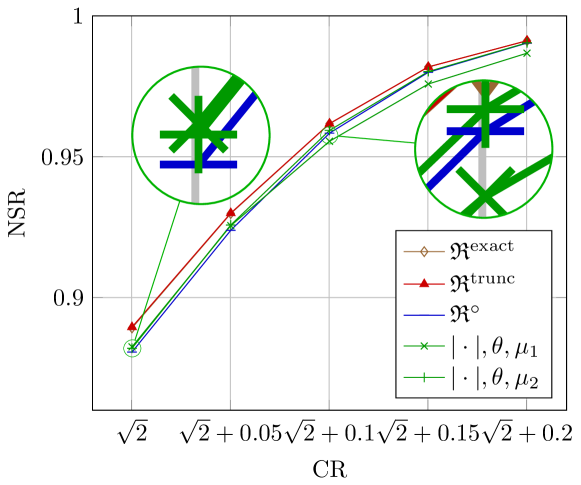
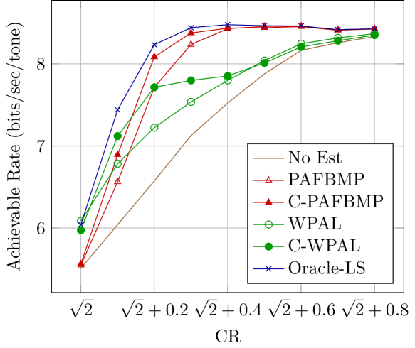
Refer to caption
Figure 9: NSR vs. CR for the various reliability functions defined in Section 4.1. Eb/N0=20subscript𝐸𝑏subscript𝑁020E_{b}/N_{0}=20dB, |Ξ©m|=64subscriptΞ©π‘š64|\Omega_{m}|=64, ΞΌ1=0.65subscriptπœ‡10.65\mu_{1}=0.65, ΞΌ2=0.95subscriptπœ‡20.95\mu_{2}=0.95.
Refer to caption
Figure 10: Achievable Rate as a function of the clipping ratio CR=Ξ³/Οƒxabsent𝛾subscript𝜎π‘₯=\gamma/\sigma_{x}.
Refer to caption
Figure 11: Relative run time (max. = 100%) at different clipping levels. mPAFBMP=0.25​Nsubscriptπ‘šPAFBMP0.25𝑁m_{\textmd{PAFBMP}}=0.25N, mC-PAFBMP=0.39​Nsubscriptπ‘šC-PAFBMP0.39𝑁m_{\textmd{C-PAFBMP}}=0.39N, mWPAL=0.25​Nsubscriptπ‘šWPAL0.25𝑁m_{\textmd{WPAL}}=0.25N, mC-WPAL=0.39​Nsubscriptπ‘šC-WPAL0.39𝑁m_{\textmd{C-WPAL}}=0.39N, B=5𝐡5B=5.

5.1 Comparison of Reliability Criterias

In the first experiment, the reliability criterias proposed in this work are compared, including β„œexactsuperscriptβ„œexact\mathfrak{R}^{\text{exact}}, β„œtruncsuperscriptβ„œtrunc\mathfrak{R}^{\text{trunc}}, β„œβˆ˜superscriptβ„œ\mathfrak{R}^{\circ} and β„œβ–‘superscriptβ„œβ–‘\mathfrak{R}^{\Box}. As a performance metric, we use normalized success rate (NSR) defined as |{k:βŸ¨π’³^​(k)⟩=𝒳​(k),k∈Ωm}|/|Ξ©m|conditional-setπ‘˜formulae-sequencedelimited-⟨⟩^π’³π‘˜π’³π‘˜π‘˜subscriptΞ©π‘šsubscriptΞ©π‘š|\{k:\langle\hat{\cal X}(k)\rangle={\cal X}(k),k\in\Omega_{m}\}|/|\Omega_{m}|. The NSR depicts that among the |Ξ©m|subscriptΞ©π‘š|\Omega_{m}| tones favoured by a particular reliability criteria, how many were actually within their corresponding correct decision regions. Fig. 9 shows the result of this experiment. The results were plotted against a varying CR while 646464 most reliable carriers were sought keeping Eb/N0subscript𝐸𝑏subscript𝑁0E_{b}/N_{0} fixed at 202020dB. It is expected that as CR is increased, all reliability criterias will tend to improve. The simulation results confirm this intuition and also confirm the conjecture that the truncated reliability computation comes at little cost compared to using the exact reliability function (14). Furthermore, it is shown for the parameters used for penalizing the circular reliability function, β„œβˆ˜superscriptβ„œ\mathfrak{R}^{\circ}, by ΞΌ2=0.95subscriptπœ‡20.95\mu_{2}=0.95 (which results in a square-like function such as the curve plotted in Fig. 4 for r=0.3​dminπ‘Ÿ0.3subscript𝑑r=0.3d_{\min}) was more effective than with a smaller value of ΞΌ1=0.65subscriptπœ‡10.65\mu_{1}=0.65, for milder CR levels. On the other hand, with severe CR, smaller values of ΞΌπœ‡\mu were better. This observation is highlighted by showing enlarged version of the graph for severe and milder CRs.

5.2 Achievable Rate

In this experiment, the ultimate performance measure considered was the achievable rate with and without the proposed method. Assuming ergodicity over the subcarriers, this rate can be expressed as 1N​(βˆ‘i=0Nβˆ’1log⁑2​(1+|Ξ»i|2​σ𝒳2/(|Ξ»i|2)β€‹Οƒπ’ž2+σ𝒡2))1𝑁superscriptsubscript𝑖0𝑁121superscriptsubscriptπœ†π‘–2superscriptsubscriptπœŽπ’³2superscriptsubscriptπœ†π‘–2superscriptsubscriptπœŽπ’ž2superscriptsubscriptπœŽπ’΅2\frac{1}{N}\left(\sum_{i=0}^{N-1}\log 2(1+|\lambda_{i}|^{2}\sigma_{\cal X}^{2}/(|\lambda_{i}|^{2})\sigma_{\cal C}^{2}+\sigma_{\cal Z}^{2})\right) for the un-mitigated case, and as 1N​(βˆ‘i=0Nβˆ’1log⁑2​(1+|Ξ»i|2​σ𝒳2/(|Ξ»i|2)β€‹Οƒπ’žβˆ’π’ž^2+σ𝒡2))1𝑁superscriptsubscript𝑖0𝑁121superscriptsubscriptπœ†π‘–2superscriptsubscriptπœŽπ’³2superscriptsubscriptπœ†π‘–2superscriptsubscriptπœŽπ’ž^π’ž2superscriptsubscriptπœŽπ’΅2\frac{1}{N}\left(\sum_{i=0}^{N-1}\log 2(1+|\lambda_{i}|^{2}\sigma_{\cal X}^{2}/(|\lambda_{i}|^{2})\sigma_{{\cal C}-\hat{\cal C}}^{2}+\sigma_{\cal Z}^{2})\right), for the case when an estimate 𝓒^bold-^𝓒\bm{\hat{\mathcal{C}}} of 𝓒𝓒\bm{\mathcal{C}} is obtained by an arbitrary method [2]. As a benchmark Oracle-LS is utilized, where the support of clipping signal is perfectly known and the active elements are estimated using LS estimate at the receiver. By using the WPAL (11)[6] and PAFBMP [11] sparse recovery algorithms over the exact reliability function β„œexactsuperscriptβ„œexact\mathfrak{R}^{\text{exact}}, we compared the clipping mitigation results. The results in Fig. 10 show the superior performance of C-PAFBMP [11] using the most reliable 39%percent3939\% of carriers and the ability of C-WPAL to beat all the techniques at CRs around 1.51.51.5 using the most reliable 39%percent3939\% carriers.

5.3 Complexity

A practical comparison of relative run times for the tested algorithms is reported in Fig. 11. All times are scaled and represented as percentage of the maximum time required for recovery. We observe that PAFBMP has the least complexity among the compared schemes and this complexity reduces with increased CR.

6 Conclusion

A novel method for nonlinear distortion mitigation using pilotless sparse recovery techniques was proposed. The method exploits the sparsity of the distortion in time domain to fully recover the signal without being influenced by incorrect ML-decoding decisions. The method adaptively senses over reliable subsets of observations of the distortion in frequency domain to perform the recovery. A new method of computing the reliability of each observation independently of the other Mβˆ’1𝑀1M-1 candidates within a constellation was also proposed and tested. Through simulations, it is verified that the proposed scheme provides favourable results for clipping signal recovery and achieves a rate close to Oracle-LS based recovery.

Appendix A Deriving fπ’Ÿsubscriptπ‘“π’Ÿf_{{\cal D}}

Beginning with the fact that

Οƒπ’Ÿ2=Οƒπ’ž2+Ξ»βˆ’π–§β€‹Ξ»βˆ’1​σ𝒡2,superscriptsubscriptπœŽπ’Ÿ2superscriptsubscriptπœŽπ’ž2superscriptπœ†π–§superscriptπœ†1superscriptsubscriptπœŽπ’΅2\displaystyle\sigma_{{\cal D}}^{2}=\sigma_{{\cal C}}^{2}+\lambda^{-{\sf H}}\lambda^{-1}\sigma_{{\cal Z}}^{2}, (35)

can be made, and we subsequently work out the energy of the sparse vector, 𝒄𝒄{\bm{c}}, which is a compound random variable. By total expectation we have

𝔼[βˆ₯𝒄βˆ₯22]=𝔼|ℐc|[𝔼[βˆ₯𝒄βˆ₯22||ℐ𝒄|]]=𝔼|ℐ𝒄|[|ℐ𝒄|𝔼[|c|2]]=𝔼[|ℐ𝒄|]𝔼[|c|2]\displaystyle\mathbb{E}\left[\|{\bm{c}}\|_{2}^{2}\right]=\mathbb{E}_{\,|{\cal I}_{c}|}\left[\mathbb{E}\left[\|{\bm{c}}\|_{2}^{2}\big{|}|{\cal I}_{{\bm{c}}}|\right]\right]=\mathbb{E}_{\,|{\cal I}_{{\bm{c}}}|}\left[|{\cal I}_{{\bm{c}}}|\mathbb{E}\left[|c|^{2}\right]\right]=\mathbb{E}\left[|{\cal I}_{{\bm{c}}}|\right]\mathbb{E}\left[|c|^{2}\right] (36)

where we have dropped the index in 𝔼​[|c|2]𝔼delimited-[]superscript𝑐2\mathbb{E}\left[|c\,|^{2}\right] to denote an arbitrary nonzero coefficient of 𝒄𝒄{\bm{c}}. Using this result, we can see that Οƒπ’ž2=𝔼​[‖𝒄‖22]/N=𝔼​[|c|2]​𝔼​[|ℐ𝒄|]/NsuperscriptsubscriptπœŽπ’ž2𝔼delimited-[]superscriptsubscriptnorm𝒄22𝑁𝔼delimited-[]superscript𝑐2𝔼delimited-[]subscriptℐ𝒄𝑁\sigma_{{\cal C}}^{2}=\mathbb{E}[\|{\bm{c}}\|_{2}^{2}]/N=\mathbb{E}[|c|^{2}]\mathbb{E}[|{\cal I}_{{\bm{c}}}|]/N by Parseval’s energy conservation law and an ergodicity assumption. Moreover,

𝔼[|c|2]=𝔼[|x|2||x|>Ξ³]βˆ’2γ𝔼[|x|||x|>Ξ³]+Ξ³2\displaystyle\mathbb{E}[|c|^{2}]=\mathbb{E}\left[|x|^{2}\big{|}|x|>\gamma\right]-2\gamma\mathbb{E}\left[|x|\big{|}|x|>\gamma\right]+\gamma^{2} (37)

and so we derive the pdf of |x|π‘₯|x| given |x|>Ξ³π‘₯𝛾|x|>\gamma to be

f(|x|||x|>Ξ³)=f​(|x|)​δ​(|x|βˆ’Ξ³)𝔽¯|x|2​(Ξ³)=|x|Οƒ|x|2eβˆ’|x|2+Ξ³22​σ|x|2Ξ΄(|x|βˆ’Ξ³)\displaystyle f\left(|x|\big{|}|x|>\gamma\right)=\frac{f\left(|x|\right)\delta(|x|-\gamma)}{\bar{\mathbb{F}}^{2}_{|x|}(\gamma)}=\frac{|x|}{\sigma_{|x|}^{2}}e^{\frac{-|x|^{2}+\gamma^{2}}{2\sigma_{|x|}^{2}}}\delta(|x|-\gamma) (38)

where 𝔽¯|x|​(Ξ³)=eβˆ’Ξ³22​σ|x|2subscript¯𝔽π‘₯𝛾superscript𝑒superscript𝛾22superscriptsubscript𝜎π‘₯2\bar{\mathbb{F}}_{|x|}(\gamma)=e^{\frac{-\gamma^{2}}{2\sigma_{|x|}^{2}}}. Computing the terms in (37) using (38) we get

𝔼​[|c|2]=2​σ|x|2βˆ’2​π2​γ​σ|x|​eΞ³22​σ|x|2​(1βˆ’erf​(Ξ³2​σ|x|))𝔼delimited-[]superscript𝑐22superscriptsubscript𝜎π‘₯22πœ‹2𝛾subscript𝜎π‘₯superscript𝑒superscript𝛾22superscriptsubscript𝜎π‘₯21erf𝛾2subscript𝜎π‘₯\displaystyle\mathbb{E}[|c|^{2}]=2\sigma_{|x|}^{2}-2\sqrt{\frac{\pi}{2}}\gamma\sigma_{|x|}e^{\frac{\gamma^{2}}{2\sigma_{|x|}^{2}}}\left(1-\textmd{erf}\left(\frac{\gamma}{\sqrt{2}\sigma_{|x|}}\right)\right) (39)

Lastly, since |ℐ𝒄|subscriptℐ𝒄|{\cal I}_{{\bm{c}}}| is a binomial, 𝔼​[|ℐ𝒄|]=N​𝔽¯|x|​(Ξ³)=N​eβˆ’Ξ³22​σ|x|2𝔼delimited-[]subscriptℐ𝒄𝑁subscript¯𝔽π‘₯𝛾𝑁superscript𝑒superscript𝛾22superscriptsubscript𝜎π‘₯2\mathbb{E}[|{\cal I}_{{\bm{c}}}|]=N\bar{\mathbb{F}}_{|x|}(\gamma)=Ne^{\frac{-\gamma^{2}}{2\sigma_{|x|}^{2}}}. Substituting these last two expressions into (36) gives Οƒπ’ž2superscriptsubscriptπœŽπ’ž2\sigma_{{\cal C}}^{2}, which in turn produces (35), and this parameter characterizes fπ’Ÿsubscriptπ‘“π’Ÿf_{{\cal D}}.

Appendix B Tailoring the Lambert 𝒲𝒲\mathcal{W}-Function

Given the equation y=x​ex𝑦π‘₯superscript𝑒π‘₯y=xe^{x}, which for reasons stated below we call the canonical form, it is desired to solve explicitly for xπ‘₯x. Unfortunately, this could not be done using elementary operations. Instead, the solution can be expressed in terms of the Lambert 𝒲𝒲{\cal W}-Function, where x=𝒲​(y)π‘₯𝒲𝑦x={\cal W}(y) is the solution to the canonical form, and where we can thus equivalently write y=𝒲​(y)​e𝒲​(y)𝑦𝒲𝑦superscript𝑒𝒲𝑦y={\cal W}(y)e^{{\cal W}(y)}.

The function is generally multivalued. If we restrict its argument, y𝑦y, to be real, then it produces two outputs for each point on the supporting interval y∈[βˆ’eβˆ’1,0]𝑦superscript𝑒10y\in[-e^{-1},0], which is our interval of interest. However, one of the two outputs of 𝒲​(y)𝒲𝑦{\cal W}(y) is β‰₯βˆ’1absent1\geq-1, and is referred to as the primary branch, 𝒲0​(y)subscript𝒲0𝑦{\cal W}_{0}(y), while the second is <βˆ’1absent1<-1, and is referred to as the secondary branch, π’²βˆ’1​(y)subscript𝒲1𝑦{\cal W}_{-1}(y). It will soon be clear that only the primary branch is needed (hence an injective mapping between y𝑦y and xπ‘₯x is retained). In any case, the function can be found iteratively by Newton’s method; for instance, xj+1=xjβˆ’xj​exjβˆ’yexj+xj​exjsubscriptπ‘₯𝑗1subscriptπ‘₯𝑗subscriptπ‘₯𝑗superscript𝑒subscriptπ‘₯𝑗𝑦superscript𝑒subscriptπ‘₯𝑗subscriptπ‘₯𝑗superscript𝑒subscriptπ‘₯𝑗x_{j+1}=x_{j}-\frac{x_{j}e^{x_{j}}-y}{e^{x_{j}}+x_{j}e^{x_{j}}}. The problem at hand, as expressed in (22), is more complex than the canonical form. Nonetheless, it could be reduced to this form by a clever substitution [14]. First express (22) compactly as

ea​r~+b=c​r~+d,superscriptπ‘’π‘Ž~π‘Ÿπ‘π‘~π‘Ÿπ‘‘\displaystyle e^{a\tilde{r}+b}=c\tilde{r}+d, (40)

where a=2​dmin/ΟƒD2π‘Ž2subscript𝑑superscriptsubscript𝜎𝐷2a=\sqrt{2}d_{\min}/\sigma_{D}^{2}, b=βˆ’dmin2/ΟƒD2𝑏superscriptsubscript𝑑2superscriptsubscript𝜎𝐷2b=-d_{\min}^{2}/\sigma_{D}^{2}, c=2​dmin/ΟƒD2=a𝑐2subscript𝑑superscriptsubscript𝜎𝐷2π‘Žc=\sqrt{2}d_{\min}/\sigma_{D}^{2}=a, and d=βˆ’1𝑑1d=-1. Letting ρ=βˆ’a​(r+dc)πœŒπ‘Žπ‘Ÿπ‘‘π‘\rho=-a(r+\frac{d}{c}) and substituting into (40) gives βˆ’ac​eβˆ’a​dc+b=ρ​eΟπ‘Žπ‘superscriptπ‘’π‘Žπ‘‘π‘π‘πœŒsuperscriptπ‘’πœŒ-\frac{a}{c}e^{-\frac{ad}{c}+b}=\rho e^{\rho}. Comparing with the canonical form, the solution to the equation can be expressed as ρ=𝒲0​(βˆ’ac​eβˆ’a​dc+b)𝜌subscript𝒲0π‘Žπ‘superscriptπ‘’π‘Žπ‘‘π‘π‘\rho={\cal W}_{0}(-\frac{a}{c}e^{-\frac{ad}{c}+b}). Back-substitution to the four parameters in (40) returns r~=βˆ’1a​𝒲0​(βˆ’ac​eβˆ’a​dc+b)βˆ’dc~π‘Ÿ1π‘Žsubscript𝒲0π‘Žπ‘superscriptπ‘’π‘Žπ‘‘π‘π‘π‘‘π‘\tilde{r}=-\frac{1}{a}{\cal W}_{0}\left(-\frac{a}{c}e^{-\frac{ad}{c}+b}\right)-\frac{d}{c}. Returning the values of a,b,cπ‘Žπ‘π‘a,b,c and d𝑑d into this equation gives the final expression in (23).

References

  • [1] E.Β B. Al-Safadi and T.Β Y. Al-Naffouri. Pilotless recovery of clipped OFDM signals by compressive sensing over reliable data carriers. In Proc. SPAWC, pages 580–584. IEEE, 2012.
  • [2] J.Β Tellado. Multicarrier modulation with low PAR: applications to DSL and wireless. Springer, 2000.
  • [3] J.-C. Chen and C.-P. Li. Tone reservation using near-optimal peak reduction tone set selection algorithm for PAPR reduction in OFDM systems. IEEE Signal Process. Lett., 17(11):933–936, 2010.
  • [4] N.Β Andgart etΒ al. Designing tone reservation PAR reduction. EURASIP J. Appl. Signal Process., 2006, 2006.
  • [5] B.S. Krongold, D.L. JonesB.Β S. Krongold, and D.Β L. Jones. An active-set approach for OFDM PAR reduction via tone reservation. IEEE Trans. Signal Process., 52(2):495–509, 2004.
  • [6] E.Β B. Al-Safadi and T.Β Y. Al-Naffouri. Peak reduction and clipping mitigation in OFDM by augmented compressive sensing. IEEE Trans. Signal Process., 60(7):3834–3839, 2012.
  • [7] M.Β Mohammadnia-Avval, A.Β Ghassemi, and L.Β Lampe. Compressive sensing recovery of nonlinearly distorted OFDM signals. In Proc. ICC, pages 1–5. IEEE, 2011.
  • [8] E.Β J. CandΓ¨s, J.Β Romberg, and T.Β Tao. Robust uncertainty principles: Exact signal reconstruction from highly incomplete frequency information. IEEE Trans. Inf. Theory, 52(2):489–509, 2006.
  • [9] E.Β J. CandΓ¨s and T.Β Tao. Near-optimal signal recovery from random projections: Universal encoding strategies? IEEE Trans. Inf. Theory, 52(12):5406–5425, 2006.
  • [10] R.Β Tibshirani. Regression shrinkage and selection via the LASSO. J. Roy. Stat. Soc. Ser. B Stat. Methodol., Series B, 58:267–288, 1996.
  • [11] P.Β Schniter, L.Β C. Potter, and J.Β Ziniel. Fast Bayesian matching pursuit. In Workshop on Inf. Theory and Appl., pages 326–333. IEEE, 2008.
  • [12] H.Β A. David and H.Β N. Nagaraja. Order statistics. Wiley Online Library, 1970.
  • [13] O.Β Edfors etΒ al. OFDM channel estimation by singular value decomposition. IEEE Trans. Commun., 46(7):931–939, 1998.
  • [14] R.Β M. Corless etΒ al. On the Lambert W function. Adv. in Comput. Math., 5(1):329–359, 1996.
  • [15] S.Β Prot, M.Β Flanagan, and C.Β Heneghan. Conditional Quasi Maximum Likelihood Receiver for Clipped OFDM Signals. In Proc. ECCTD, 2005.
  • [16] R.Β E. Carrillo, K.Β E. Barner, and T.Β C. Aysal. Robust sampling and reconstruction methods for sparse signals in the presence of impulsive noise. IEEE J. Sel. Topics Signal Process., 4(2):392–408, 2010.
  • [17] C.-T. Lin and W.-R. Wu. Clipping ratio estimation for OFDM receivers. In Proc. IEEE Veh. Technol. Conf., volumeΒ 2, pages 797–800. IEEE, 2005.
  • [18] M.Β Grantand, S.Β Boyd, and Y.Β Ye. Cvx: Matlab software for disciplined convex programming. http://cvxr.com/cvx, 2008.