Linearized averaged resonant equations and their solution for dust particles

Abstract

The averaged resonant equations of motion for the planar circular restricted three-body problem are solved on the linearization basis taking into account also non-gravitational effects. The averaged resonant equations are derived from Lagrange’s planetary equations with additional Gauss’s terms caused by the non-gravitational effects. The time depending solution has the standard form with exponential, quadratic, linear and constant terms. The existence of a rotational symmetry in the action of the non-gravitational effects around the star determines the order of a characteristic equation of the linearized system. In the symmetrical case (order 3) the considered non-gravitational effects are the stellar electromagnetic radiation and the radial stellar wind (stellar radiation). In the asymmetrical case (order 4) the stellar radiation and interstellar gas flow are considered. It is investigated how well the linearization solution describes real solution obtained from an equation of motion by a comparison of the resonant libration frequency found analytically and numerically. It is found that from initial values of the evolving orbital parameters (semimajor axis, eccentricity, longitude of pericenter, and resonant angular variable) in the averaged phase space the linearization frequency depends most sensitively on the initial value of the resonant angular variable. For small libration amplitudes of the resonant angular variable the best match of the real libration frequency and the linearization frequency is located approximately at the solution of the resonant condition ($da/dt$ $=$ 0). If the initial averaged conditions are chosen close to the solution of resonant condition, then the linearization frequency for practically all simple oscillatory evolutions matches the real libration frequency and the linearization solution very well approximates the real evolution. The linearization results obtained for stationary solutions are tested. In the planar circular restricted Sun-Neptune-dust problem with the solar radiation and the interstellar gas flow the solutions of resonant condition are practically independent on the longitude of perihelion.

1 Introduction

The gravity of a star and a planet that move according to a solution of the two body problem disturbs the motion of a body with negligible mass (restricted three-body problem). The dynamics of the body with negligible mass includes in this case also the so called mean motion resonances. In a mean motion resonance a ratio of orbital periods of the two minor bodies oscillates near a ratio of two natural numbers. The motion of the body with negligible mass in the mean motion resonance cannot be solved completely even in the planar case (when the motions are confined to one plane). Several approximative solutions for an averaged problem can be found in the literature. The behavior predicted by the averaged solutions depends on the period of averaging. After the averaging over a synodic period oscillations in the evolution of semimajor axis should be present. The oscillations are also present if the averaged solution is determined using Fourier series expansion of the disturbing function with considered single resonant term (e.g. Greenberg, 1973; Murray & Dermott, 1999). After the averaging over the libration period the semimajor axis should be constant.

Greenberg (1973) substituted the truncated averaged Fourier series expansion of the disturbing function in the time derivatives of orbital elements given by Lagrange’s planetary equations. Lagrange’s planetary equations for the planar circular restricted three-body problem (PCRTBP) including a tidal dissipation were solved simultaneously using several approximations. Another example of the time dependence obtained using the truncated Fourier series of the disturbing function can be found in Murray & Dermott (1999). By individual time integration of Lagrange’s planetary equations in the PCRTBP with substituted single resonant term from the Fourier series they obtained dependencies of orbital elements on time. They assumed that the only time-varying quantities in the equations are in the trigonometric arguments of the resonant term and that the longitude of perihelion increases linearly with time at a constant rate determined by secular theory. Evolutions obtained from Fourier series expansion of the disturbing function will be no more discussed in this paper.

The evolutions averaged over the libration period are commonly used for the description of the long term evolution of dust particles captured in the mean motion resonances with the planet. The dust particles captured in a neighborhood of the Earth’s orbit were predicted by Jackson & Zook (1989) and observed in the infrared light by the satellites IRAS (Dermott et al., 1994) and COBE (Reach et al., 1995). The dust particles are significantly influenced by non-gravitational effects. When the resonant dust particles are under the action of the Poynting–Roberson (PR) effect (Poynting, 1904; Robertson, 1937; Burns et al., 1979; Klačka, 2004; Klačka et al., 2014) and a radial solar wind (Klačka et al., 2012), then the evolution of eccetrtricity averaged over the libration period shows a sorted monotonic behavior. Properties of this behavior were investigated in some depth by Weidenschilling & Jackson (1993); Beaugé & Ferraz-Mello (1994); Gomes (1995); Liou et al. (1995); and others. After the averaging over the libration period these particles follow the eccentricity evolution described by a first order differential equation derived in Liou & Zook (1997). In Liou & Zook (1997) authors expanded the derived equation for the evolution of eccentricity to the second order in the eccentricity. The obtained equation was solved for a time dependence valid for small eccentricities. The time dependence of the eccentricity is frequently used (see e.g. Moro-Martín & Malhotra, 2002; Deller & Maddison, 2005; Krivov et al., 2007). Results obtained after the averaging over the libration period will be not taken a step further in this paper.

In Beaugé & Ferraz-Mello (1994) the equations of motion of a dust particle captured in a mean motion resonance in the PCRTBP with the PR effect were written in a near canonical form. Beaugé & Ferraz-Mello (1994) transformed the near canonical equations to a system of equations suitable for the search of stationary points and averaged them over a synodic period (averaged resonant equations). Beaugé & Ferraz-Mello (1994) linearized the averaged resonant equations around chosen stationary point and solved obtained characteristic equation of the system in order to determine a stability of the stationary points. This method was used for stability tests of the stationary points in the PCRTBP with the PR effect also by Šidlichovský & Nesvorný (1994). In Pástor (2016) periodic motions in a reference frame rotating with the planet were found to exist at each of such stationary points obtained from the averaged resonant equations. Lhotka & Celletti (2015) found stationary points in the circular-planar, spatial-circular, elliptic-planar and spatial-elliptic restricted three-body problem with the PR effect for the dust particles captured in the mean motion 1/1 resonance with the planet (see also Pástor, 2014b). The stability of found stationary points was investigated using the linearization of the equations of motion written in Delaunay variables and averaged over the orbital period.

In this paper we derive the solution of linearized averaged resonant equation for the PCRTBP with non-gravitational effect in general form. The derived solution should be valid for any mean motion resonance. The non-gravitational effects with and without the rotational symmetry around the star will be considered separately. The linearization is usually used in the literature to investigate a stability, and to search for linearization frequencies, but how well the time depending solution describes real resonant librations was not yet presented in the literature. We find that the linearization frequencies significantly depend on the initial conditions in the averaged phase space even for one libration. We show how the solution should be applied for the sake of best description of almost all evolutions with simple oscillations in the mean motion resonances. Frequencies for periodic solutions in exterior mean motion 6/5, 7/6, 8/7, and 9/8 resonances with the Earth in a circular orbit will be determined. The applicability will be investigated when the non-gravitational effects are the PR effect, radial solar wind and interstellar gas flow.

2 Averaged resonant equations

For the study of a specific mean motion resonance it is convenient to define a resonant angular variable (e.g. Greenberg, 1973; Beaugé & Ferraz-Mello, 1993, 1994; Gomes, 1995)

$$\sigma=\frac{p+q}{q}\lambda_{\text{P}}-s\lambda-\tilde{\omega}~{},$$ (1)

here $p$ and $q$ are two integers (resonant numbers), $\lambda_{\text{P}}$ is the mean longitude of the planet in a circular orbit, $\lambda$ is the mean longitude of the dust particle, $\tilde{\omega}$ is the longitude of pericenter, and $s$ $=$ $p/q$. In what follows we will need also the time derivative of the resonant angular variable. The mean longitude of the planet increases linearly with the time $t$ from its initial value $\lambda_{\text{P}0}$ with a constant slope equal to the mean motion of the planet $n_{\text{P}}$ ($\lambda_{\text{P}}$ $=$ $n_{\text{P}}t$ $+$ $\lambda_{\text{P}0}$). We define an angle $\sigma_{\text{b}}$ so that the mean anomaly of the dust particle can be computed from the relation $M$ $=$ $nt$ $+$ $\sigma_{\text{b}}$ using the mean motion of the particle $n$ and the time (Bate et al., 1971). The mean motion of the particle with the negligible mass is given by the third Kepler’s law $n$ $=$ $\sqrt{\mu/a^{3}}$, here $\mu$ $=$ $G_{0}M_{\star}$, $G_{0}$ is the gravitational constant, $M_{\star}$ is the mass of the star, and $a$ is the semimajor axis of the particle’s orbit. The mean longitude of the dust particle is according to the definitions above $\lambda$ $=$ $M$ $+$ $\tilde{\omega}$ $=$ $nt$ $+$ $\sigma_{\text{b}}$ $+$ $\tilde{\omega}$. In the mean motion resonance $\sigma$ is librating rather than circulating. For the time derivative of $\sigma$ we have

$$\frac{d\sigma}{dt}=\frac{p+q}{q}n_{\text{P}}-sn-s\left(\frac{d\sigma_{\text{b}}}{dt}+t\frac{dn}{dt}+\frac{d\tilde{\omega}}{dt}\right)-\frac{d\tilde{\omega}}{dt}~{}.$$ (2)

Short periodic variations in the evolution during the mean motion resonance can be ignored in the most practical cases. This can be done effectively by an averaging over a synodic period. The synodic period is determined by a difference in mean longitudes of the planet and the particle, and the order of resonance $q$ in the angle variable

$$\sigma_{\text{T}}=\frac{\lambda-\lambda_{\text{P}}}{q}~{}.$$ (3)

The difference between $\sigma_{\text{T}}$ at time zero and $\sigma_{\text{T}}$ after one synodic period is equal to $2\pi$.

The orbital evolution of a dust particle is significantly influenced also by non-gravitational effects. For the non-gravitational effects that slowly vary the dust particle’s orbit the long term (secular) orbital evolution can be described by the averaged time derivatives of the orbital elements. The averaged time derivatives can be calculated using Gauss’s perturbation equations of celestial mechanics (e.g. Danby, 1988; Murray & Dermott, 1999). The secular time derivatives of the orbital elements caused by the planet can be calculated using Lagrange’s planetary equations averaged over the synodic period (Brouwer & Clemence, 1961; Danby, 1988). After the averaging we can sum Lagrange’s planetary equations and Gauss’s perturbation equations in order to obtain the system of equations describing the secular orbital evolution of the dust particle. In the planar case the equations are

$$\frac{da}{dt} =\frac{2a}{L}\frac{\partial R}{\partial\sigma_{\text{b}}}+\left(\frac{da}{dt}\right)_{\text{EF}}~{},$$

$$\frac{de}{dt} =\frac{\alpha^{2}}{Le}\frac{\partial R}{\partial\sigma_{\text{b}}}-\frac{\alpha}{Le}\frac{\partial R}{\partial\tilde{\omega}}+\left(\frac{de}{dt}\right)_{\text{EF}}~{},$$

$$\frac{d\tilde{\omega}}{dt} =\frac{\alpha}{Le}\frac{\partial R}{\partial e}+\left(\frac{d\tilde{\omega}}{dt}\right)_{\text{EF}}~{},$$

$$\frac{d\sigma_{\text{b}}}{dt}+t\frac{dn}{dt} =-\frac{2a}{L}\frac{\partial R}{\partial^{\star}a}-\frac{\alpha^{2}}{Le}\frac{\partial R}{\partial e}+\left(\frac{d\sigma_{\text{b}}}{dt}+t\frac{dn}{dt}\right)_{\text{EF}}~{}.$$ (4)

Here $L$ $=$ $\sqrt{\mu a}$, $e$ is the eccentricity, and $\alpha$ $=$ $\sqrt{1-e^{2}}$. $R$ is the disturbing function of the PCRTBP

$$R=G_{0}M_{\text{P}}\left(\frac{1}{|\vec{r}-\vec{r}_{\text{P}}|}-\frac{\vec{r}\cdot\vec{r}_{\text{P}}}{r_{\text{P}}^{3}}\right)$$ (5)

with its partial derivatives in Eqs. (2) averaged over the synodic period. In the disturbing function: $M_{\text{P}}$ is the mass of the planet, $\vec{r}_{\text{P}}$ is the position vector of the planet with respect to the star, $r_{\text{P}}$ $=$ $|\vec{r}_{\text{P}}|$, and $\vec{r}$ is the position vector of the dust particle with respect to the star. The subscript EF in Eqs. (2) denotes the terms that are caused by the non-gravitational effects only. $\partial R/\partial^{\star}a$ in the last equation in Eqs. (2) denotes that the partial derivative of the disturbing function with respect to the semimajor axis is calculated with an assumption that the mean motion of the particle $n$ is not a function of the semimajor axis. This can be shown in the un-averaged phase space since we have

$$\left(\frac{d\sigma_{\text{b}}}{dt}\right)_{\text{G}} =-\frac{2a}{L}\frac{\partial R}{\partial a}-\frac{\alpha^{2}}{Le}\frac{\partial R}{\partial e}=-\frac{2a}{L}\frac{\partial R}{\partial^{\star}a}-\frac{\alpha^{2}}{Le}\frac{\partial R}{\partial e}-\frac{2a}{L}\frac{\partial R}{\partial\sigma_{\text{b}}}t\frac{\partial n}{\partial a}$$

$$=-\frac{2a}{L}\frac{\partial R}{\partial^{\star}a}-\frac{\alpha^{2}}{Le}\frac{\partial R}{\partial e}-\left(t\frac{dn}{dt}\right)_{\text{G}}~{}.$$ (6)

The subscript G denotes the terms that are caused by the gravitation only. In Eqs. (2) we have substituted also the un-averaged gravitational part of the first equation in Eqs. (2). Using Eqs. (2) averaged over the synodic period, we can obtain the last equation in Eqs. (2) as follows

$$\frac{d\sigma_{\text{b}}}{dt}+t\frac{dn}{dt} =\left(\frac{d\sigma_{\text{b}}}{dt}\right)_{\text{G}}+\left(\frac{d\sigma_{\text{b}}}{dt}\right)_{\text{EF}}+\left(t\frac{dn}{dt}\right)_{\text{G}}+\left(t\frac{dn}{dt}\right)_{\text{EF}}$$

$$=-\frac{2a}{L}\frac{\partial R}{\partial^{\star}a}-\frac{\alpha^{2}}{Le}\frac{\partial R}{\partial e}+\left(\frac{d\sigma_{\text{b}}}{dt}+t\frac{dn}{dt}\right)_{\text{EF}}~{}.$$ (7)

Equations (2) already describe the secular evolution of the dust particle captured in the mean motion resonance and simultaneously affected by the non-gravitational effects.

The secular evolution in a specific resonance given by the resonant numbers $p$ and $q$ cannot be easily seen in Eqs. (2). In order to study the resonances we transform Eqs. (2) as follows. Equation (2) can be averaged over the synodic period. If we use in the averaged result the last two equations in Eqs. (2), then we get

$$\frac{d\sigma}{dt}={} -\frac{\alpha}{Le}\left[1+s\left(1-\alpha\right)\right]\frac{\partial R}{\partial e}+\frac{2sa}{L}\frac{\partial R}{\partial^{\star}a}+n_{\text{P}}\frac{p+q}{q}-ns$$

$$-\frac{p+q}{q}\left(\frac{d\tilde{\omega}}{dt}\right)_{\text{EF}}-s\left(\frac{d\sigma_{\text{b}}}{dt}+t\frac{dn}{dt}\right)_{\text{EF}}~{}.$$ (8)

The partial derivatives of the disturbing function $R$ averaged over the synodic period are not functions of $\tilde{\omega}$ they are only functions of $a$, $e$, and $\sigma$. Between averaged partial derivatives of the disturbing function $R$ the following relations hold

$$\frac{\partial R}{\partial\sigma_{\text{b}}} =-s\frac{\partial R}{\partial\sigma}~{},$$

$$\frac{\partial R}{\partial\tilde{\omega}} =-\frac{p+q}{q}\frac{\partial R}{\partial\sigma}~{}.$$ (9)

We can use Eqs. (2) in the first two equations in the system of equations given by Eqs. (2). The last equation in Eqs. (2) can be replaced with equivalent Eq. (2). By this we obtain a system that enables the study of the secular evolution of the dust particle captured in the specific mean motion resonance given by the resonant numbers $p$ and $q$ under the action of the non-gravitational effects

$$\frac{da}{dt}={} -\frac{2sa}{L}\frac{\partial R}{\partial\sigma}+\left(\frac{da}{dt}\right)_{\text{EF}}~{},$$

$$\frac{de}{dt}={} \frac{\alpha}{Le}\left[1+s\left(1-\alpha\right)\right]\frac{\partial R}{\partial\sigma}+\left(\frac{de}{dt}\right)_{\text{EF}}~{},$$

$$\frac{d\tilde{\omega}}{dt}={} \frac{\alpha}{Le}\frac{\partial R}{\partial e}+\left(\frac{d\tilde{\omega}}{dt}\right)_{\text{EF}}~{},$$

$$\frac{d\sigma}{dt}={} -\frac{\alpha}{Le}\left[1+s\left(1-\alpha\right)\right]\frac{\partial R}{\partial e}+\frac{2sa}{L}\frac{\partial R}{\partial^{\star}a}+n_{\text{P}}\frac{p+q}{q}-ns$$

$$-\frac{p+q}{q}\left(\frac{d\tilde{\omega}}{dt}\right)_{\text{EF}}-s\left(\frac{d\sigma_{\text{b}}}{dt}+t\frac{dn}{dt}\right)_{\text{EF}}~{}.$$ (10)

Equations (2) still valid also close to the zero eccentricity. Singularities in the eccentricity reflect noncontinuous behavior in the evolutions at the zero eccentricity. For example, it is possible that a decrease of the eccentricity does change suddenly to an increase at the zero eccentricity. Singularities in eccentricities reflect also definitions of the orbital elements. For example, the longitude of pericenter is not defined at the zero eccentricity. The last term in Eqs. (2) despite of its complicated appearance can be straightforwardly obtained using (Bate et al., 1971)

$$\left(\frac{d\sigma_{\text{b}}}{dt}+t\frac{dn}{dt}\right)_{\text{EF}}=\left(\frac{dM}{dt}-n\right)_{\text{EF}}={} \biggl{\langle}\frac{1-e^{2}}{na}\biggl{[}a_{\text{R}}\left(\frac{\cos f}{e}-\frac{2}{1+e\cos f}\right)$$

$$-a_{\text{T}}\frac{\sin f}{e}\frac{2+e\cos{f}}{1+e\cos f}\biggr{]}\biggr{\rangle}~{},$$ (11)

where $f$ is the true anomaly, $a_{\text{R}}$ and $a_{\text{T}}$ are the radial and transversal components of the acceleration caused by the non-gravitational effects. The angle brackets in Eq. (2) denote an averaging over one orbital period $T$ (see e.g. Klačka, 2004)

$$\langle g\rangle=\frac{1}{T}\int_{0}^{T}g(t)~{}dt=\frac{1}{T}\int_{0}^{2\pi}g(f)~{}\frac{dt}{df}~{}df=\frac{1}{2\pi a^{2}\sqrt{1-e^{2}}}\int_{0}^{2\pi}r^{2}~{}g(f)~{}df.$$ (12)

The system of equations given by Eqs. (2) is different from systems considered in Beaugé & Ferraz-Mello (1994) and Šidlichovský & Nesvorný (1994). Equations (8) in Beaugé & Ferraz-Mello (1994) are equivalent with Eqs. (2) if

$$\left(\frac{d\tilde{\omega}}{dt}\right)_{\text{EF}}={} 0~{},$$

$$\left(\frac{d\sigma_{\text{b}}}{dt}+t\frac{dn}{dt}\right)_{\text{EF}}={} 0~{}.$$ (13)

Similarly as for the system of equations in Beaugé & Ferraz-Mello (1994) Eqs. (18) in Šidlichovský & Nesvorný (1994) include only the non-gravitational effects for which Eqs. (2) hold. Šidlichovský & Nesvorný (1994) have only three equations in the system. The evolution of the longitude of pericenter is ignored in Šidlichovský & Nesvorný (1994). The equations of motion in this paper (Eqs. 2) are usable also for the non-gravitational effects that can have non-zero secular variations on the left-hand side of Eqs. (2). This property make them usable also for the non-gravitational effects acting without a rotational symmetry around the star (see Appendix A in Pástor, 2016).

3 Linearization of averaged resonant equations

No general method exists for solving nonlinear differential equations in the system Eqs. (2). If another method (use of nonlinear coordinate transformations, Lie transformations, etc.) does not allow go further, then the best that can be accomplished (Ames, 1977) is to study a linearization based upon initial conditions for the function and its derivatives. In the vicinity of an initial point $a_{0}$, $e_{0}$, $\tilde{\omega}_{0}$, and $\sigma_{0}$ we use notation

$$\delta_{a} =a-a_{0}~{},$$

$$\delta_{e} =e-e_{0}~{},$$

$$\delta_{\tilde{\omega}} =\tilde{\omega}-\tilde{\omega}_{0}~{},$$

$$\delta_{\sigma} =\sigma-\sigma_{0}~{}.$$ (14)

The time will be measured from an initial time $t_{0}$ $=$ 0. Hence

$$\delta_{t}=t~{}.$$ (15)

On the left-hand side of Eqs. (2) we substitute identities from Eqs. (3). Then for example, the time derivative of the semimajor axis can be written as follows

$$\frac{da}{dt}=\frac{d}{dt}(\delta_{a}+a_{0})=\frac{d\delta_{a}}{dt}~{}.$$ (16)

The linearization of averaged resonant equations in the used notation is

$$\frac{d\delta_{a}}{dt}{} ={} \biggl{[}\frac{\partial}{\partial^{\star}a}{} \left(\frac{da}{dt}\right)\biggr{]}_{0}{} \delta_{a}{} +{} \biggl{[}\frac{\partial}{\partial e}{} \left(\frac{da}{dt}\right)\biggr{]}_{0}{} \delta_{e}{} +{} \biggl{[}\frac{\partial}{\partial\tilde{\omega}}\left(\frac{da}{dt}\right)\biggr{]}_{0}\delta_{\tilde{\omega}}$$

$$+{} \biggl{[}\frac{\partial}{\partial\sigma}{} \left(\frac{da}{dt}\right)\biggr{]}_{0}{} \delta_{\sigma}{} +{} \biggl{[}\frac{\partial}{\partial t}{} \left(\frac{da}{dt}\right)\biggr{]}_{0}{} t{} +{} \left(\frac{da}{dt}\right)_{0}~{},$$

$$\frac{d\delta_{e}}{dt}{} ={} \biggl{[}\frac{\partial}{\partial^{\star}a}{} \left(\frac{de}{dt}\right)\biggr{]}_{0}{} \delta_{a}{} +{} \biggl{[}\frac{\partial}{\partial e}{} \left(\frac{de}{dt}\right)\biggr{]}_{0}{} \delta_{e}{} +{} \biggl{[}\frac{\partial}{\partial\tilde{\omega}}\left(\frac{de}{dt}\right)\biggr{]}_{0}\delta_{\tilde{\omega}}$$

$$+{} \biggl{[}\frac{\partial}{\partial\sigma}{} \left(\frac{de}{dt}\right)\biggr{]}_{0}{} \delta_{\sigma}{} +{} \biggl{[}\frac{\partial}{\partial t}{} \left(\frac{de}{dt}\right)\biggr{]}_{0}{} t{} +{} \left(\frac{de}{dt}\right)_{0}~{},$$

$$\frac{d\delta_{\tilde{\omega}}}{dt}{} ={} \biggl{[}\frac{\partial}{\partial^{\star}a}{} \left(\frac{d\tilde{\omega}}{dt}\right)\biggr{]}_{0}{} \delta_{a}{} +{} \biggl{[}\frac{\partial}{\partial e}{} \left(\frac{d\tilde{\omega}}{dt}\right)\biggr{]}_{0}{} \delta_{e}{} +{} \biggl{[}\frac{\partial}{\partial\tilde{\omega}}\left(\frac{d\tilde{\omega}}{dt}\right)\biggr{]}_{0}\delta_{\tilde{\omega}}$$

$$+{} \biggl{[}\frac{\partial}{\partial\sigma}{} \left(\frac{d\tilde{\omega}}{dt}\right)\biggr{]}_{0}{} \delta_{\sigma}{} +{} \biggl{[}\frac{\partial}{\partial t}{} \left(\frac{d\tilde{\omega}}{dt}\right)\biggr{]}_{0}{} t{} +{} \left(\frac{d\tilde{\omega}}{dt}\right)_{0}~{},$$

$$\frac{d\delta_{\sigma}}{dt}{} ={} \biggl{[}\frac{\partial}{\partial^{\star}a}{} \left(\frac{d\sigma}{dt}\right)\biggr{]}_{0}{} \delta_{a}{} +{} \biggl{[}\frac{\partial}{\partial e}{} \left(\frac{d\sigma}{dt}\right)\biggr{]}_{0}{} \delta_{e}{} +{} \biggl{[}\frac{\partial}{\partial\tilde{\omega}}\left(\frac{d\sigma}{dt}\right)\biggr{]}_{0}\delta_{\tilde{\omega}}$$

$$+{} \biggl{[}\frac{\partial}{\partial\sigma}{} \left(\frac{d\sigma}{dt}\right)\biggr{]}_{0}{} \delta_{\sigma}{} +{} \biggl{[}\frac{\partial}{\partial t}{} \left(\frac{d\sigma}{dt}\right)\biggr{]}_{0}{} t{} +{} \left(\frac{d\sigma}{dt}\right)_{0}~{},$$ (17)

$\partial^{\star}a$ is used here since after the averaging dependencies on $M$ in the terms with the disturbing function are lost. We calculate the derivatives with respect to the semimajor axis in the derivatives of disturbing function during the averaging at a given mean anomaly $M$ regardless of $M$ variation caused by the semimajor axis. This holds also for the eccentricity since $\partial M/\partial e$ $=$ 0 (but $\partial f/\partial e$ $\neq$ 0). The partial derivatives with respect to the time are usable only for time variations of the solved problem that are negligible during the averaging over the synodic period. The terms with the subscript 0 on the right-hand sides in Eqs. (3) are constant therefore we can simply write

$$\dot{\delta}_{a}{} ={} A_{\text{c}}\delta_{a}{} +{} B_{\text{c}}\delta_{e}{} +{} C_{\text{c}}\delta_{\tilde{\omega}}{} +{} D_{\text{c}}\delta_{\sigma}{} +{} E_{\text{c}}t{} +{} F{} ~{},{}$$

$$\dot{\delta}_{e}{} ={} G_{\text{c}}\delta_{a}{} +{} H_{\text{c}}\delta_{e}{} +{} I_{\text{c}}\delta_{\tilde{\omega}}{} +{} J_{\text{c}}\delta_{\sigma}{} +{} K_{\text{c}}t{} +{} L{} ~{},{}$$

$$\dot{\delta}_{\tilde{\omega}}{} ={} M_{\text{c}}\delta_{a}{} +{} N_{\text{c}}\delta_{e}{} +{} O_{\text{c}}\delta_{\tilde{\omega}}{} +{} P_{\text{c}}\delta_{\sigma}{} +{} Q_{\text{c}}t{} +{} R{} ~{},{}$$

$$\dot{\delta}_{\sigma}{} ={} S_{\text{c}}\delta_{a}{} +{} T_{\text{c}}\delta_{e}{} +{} U_{\text{c}}\delta_{\tilde{\omega}}{} +{} V_{\text{c}}\delta_{\sigma}{} +{} W_{\text{c}}t{} +{} X{} ~{}.{}$$ (18)

This system describes solution of system Eqs. (2) during a short time interval after the initial time $t_{0}$ $=$ 0 (see Appendix A).

It is possible to obtain an equation for one chosen variation by an elimination of the remaining variations using all equations in the system. The obtained equations for the separated variations are (see Appendix B)

$$\ddddot{\delta}_{a}{} +{} \Lambda_{a3}~{}\dddot{\delta}_{a}{} +{} \Lambda_{a2}~{}\ddot{\delta}_{a}{} +{} \Lambda_{a1}~{}\dot{\delta}_{a}{} +{} \Lambda_{a0}~{}\delta_{a}{} +{} \Lambda_{at}~{}t{} +{} \Lambda_{a}{} ={} 0~{},$$

$$\ddddot{\delta}_{e}{} +{} \Lambda_{e3}~{}\dddot{\delta}_{e}{} +{} \Lambda_{e2}~{}\ddot{\delta}_{e}{} +{} \Lambda_{e1}~{}\dot{\delta}_{e}{} +{} \Lambda_{e0}~{}\delta_{e}{} +{} \Lambda_{et}~{}t{} +{} \Lambda_{e}{} ={} 0~{},$$

$$\ddddot{\delta}_{\tilde{\omega}}{} +{} \Lambda_{\tilde{\omega}3}~{}\dddot{\delta}_{\tilde{\omega}}{} +{} \Lambda_{\tilde{\omega}2}~{}\ddot{\delta}_{\tilde{\omega}}{} +{} \Lambda_{\tilde{\omega}1}~{}\dot{\delta}_{\tilde{\omega}}{} +{} \Lambda_{\tilde{\omega}0}~{}\delta_{\tilde{\omega}}{} +{} \Lambda_{\tilde{\omega}t}~{}t{} +{} \Lambda_{\tilde{\omega}}{} ={} 0~{},$$

$$\ddddot{\delta}_{\sigma}{} +{} \Lambda_{\sigma 3}~{}\dddot{\delta}_{\sigma}{} +{} \Lambda_{\sigma 2}~{}\ddot{\delta}_{\sigma}{} +{} \Lambda_{\sigma 1}~{}\dot{\delta}_{\sigma}{} +{} \Lambda_{\sigma 0}~{}\delta_{\sigma}{} +{} \Lambda_{\sigma t}~{}t{} +{} \Lambda_{\sigma}{} ={} 0~{}.$$ (19)

In the used notation for the constants in Eqs. (3) we obtain

$$\Lambda_{3}=\Lambda_{a3}=\Lambda_{e3}=\Lambda_{\tilde{\omega}3}=\Lambda_{\sigma 3}={} -{} A_{\text{c}}{} -{} H_{\text{c}}{} -{} O_{\text{c}}{} -{} V_{\text{c}}~{},{}$$ (20)

$$\Lambda_{2}=\Lambda_{a2}=\Lambda_{e2}=\Lambda_{\tilde{\omega}2}=\Lambda_{\sigma 2}={} \left|\begin{array}[]{cc}A_{\text{c}}&B_{\text{c}}\\ G_{\text{c}}&H_{\text{c}}\\ \end{array}\right|{} +{} \left|\begin{array}[]{cc}A_{\text{c}}&C_{\text{c}}\\ M_{\text{c}}&O_{\text{c}}\\ \end{array}\right|{} +{} \left|\begin{array}[]{cc}A_{\text{c}}&D_{\text{c}}\\ S_{\text{c}}&V_{\text{c}}\\ \end{array}\right|{}$$ (27)

$$+{} \left|\begin{array}[]{cc}H_{\text{c}}&I_{\text{c}}\\ N_{\text{c}}&O_{\text{c}}\\ \end{array}\right|{} +{} \left|\begin{array}[]{cc}H_{\text{c}}&J_{\text{c}}\\ T_{\text{c}}&V_{\text{c}}\\ \end{array}\right|{} +{} \left|\begin{array}[]{cc}O_{\text{c}}&P_{\text{c}}\\ U_{\text{c}}&V_{\text{c}}\\ \end{array}\right|~{},{}$$ (34)

$$\Lambda_{1}=\Lambda_{a1}=\Lambda_{e1}=\Lambda_{\tilde{\omega}1}=\Lambda_{\sigma 1}={} -{} \left|\begin{array}[]{ccc}A_{\text{c}}&B_{\text{c}}&C_{\text{c}}\\ G_{\text{c}}&H_{\text{c}}&I_{\text{c}}\\ M_{\text{c}}&N_{\text{c}}&O_{\text{c}}\\ \end{array}\right|{} -{} \left|\begin{array}[]{ccc}A_{\text{c}}&B_{\text{c}}&D_{\text{c}}\\ G_{\text{c}}&H_{\text{c}}&J_{\text{c}}\\ S_{\text{c}}&T_{\text{c}}&V_{\text{c}}\\ \end{array}\right|{}$$ (41)

$$-{} \left|\begin{array}[]{ccc}A_{\text{c}}&C_{\text{c}}&D_{\text{c}}\\ M_{\text{c}}&O_{\text{c}}&P_{\text{c}}\\ S_{\text{c}}&U_{\text{c}}&V_{\text{c}}\\ \end{array}\right|{} -{} \left|\begin{array}[]{ccc}H_{\text{c}}&I_{\text{c}}&J_{\text{c}}\\ N_{\text{c}}&O_{\text{c}}&P_{\text{c}}\\ T_{\text{c}}&U_{\text{c}}&V_{\text{c}}\\ \end{array}\right|~{},{}$$ (48)

$$\Lambda_{0}=\Lambda_{a0}=\Lambda_{e0}=\Lambda_{\tilde{\omega}0}=\Lambda_{\sigma 0}=\left|\begin{array}[]{cccc}A_{\text{c}}&B_{\text{c}}&C_{\text{c}}&D_{\text{c}}\\ G_{\text{c}}&H_{\text{c}}&I_{\text{c}}&J_{\text{c}}\\ M_{\text{c}}&N_{\text{c}}&O_{\text{c}}&P_{\text{c}}\\ S_{\text{c}}&T_{\text{c}}&U_{\text{c}}&V_{\text{c}}\\ \end{array}\right|~{},$$ (53)

$$\Lambda_{at}{} ={} \left|\begin{array}[]{cccc}E_{\text{c}}&B_{\text{c}}&C_{\text{c}}&D_{\text{c}}\\ K_{\text{c}}&H_{\text{c}}&I_{\text{c}}&J_{\text{c}}\\ Q_{\text{c}}&N_{\text{c}}&O_{\text{c}}&P_{\text{c}}\\ W_{\text{c}}&T_{\text{c}}&U_{\text{c}}&V_{\text{c}}\\ \end{array}\right|{} ~{},~{}~{}\Lambda_{et}{} ={} \left|\begin{array}[]{cccc}A_{\text{c}}&E_{\text{c}}&C_{\text{c}}&D_{\text{c}}\\ G_{\text{c}}&K_{\text{c}}&I_{\text{c}}&J_{\text{c}}\\ M_{\text{c}}&Q_{\text{c}}&O_{\text{c}}&P_{\text{c}}\\ S_{\text{c}}&W_{\text{c}}&U_{\text{c}}&V_{\text{c}}\\ \end{array}\right|~{},{}$$ (62)

$$\Lambda_{\tilde{\omega}t}{} ={} \left|\begin{array}[]{cccc}A_{\text{c}}&B_{\text{c}}&E_{\text{c}}&D_{\text{c}}\\ G_{\text{c}}&H_{\text{c}}&K_{\text{c}}&J_{\text{c}}\\ M_{\text{c}}&N_{\text{c}}&Q_{\text{c}}&P_{\text{c}}\\ S_{\text{c}}&T_{\text{c}}&W_{\text{c}}&V_{\text{c}}\\ \end{array}\right|{} ~{},~{}~{}\Lambda_{\sigma t}{} ={} \left|\begin{array}[]{cccc}A_{\text{c}}&B_{\text{c}}&C_{\text{c}}&E_{\text{c}}\\ G_{\text{c}}&H_{\text{c}}&I_{\text{c}}&K_{\text{c}}\\ M_{\text{c}}&N_{\text{c}}&O_{\text{c}}&Q_{\text{c}}\\ S_{\text{c}}&T_{\text{c}}&U_{\text{c}}&W_{\text{c}}\\ \end{array}\right|~{}.{}$$ (71)

$$\Lambda_{a}{} ={} \left|\begin{array}[]{cccc}F_{\text{c}}&B_{\text{c}}&C_{\text{c}}&D_{\text{c}}\\ L_{\text{c}}&H_{\text{c}}&I_{\text{c}}&J_{\text{c}}\\ R_{\text{c}}&N_{\text{c}}&O_{\text{c}}&P_{\text{c}}\\ X_{\text{c}}&T_{\text{c}}&U_{\text{c}}&V_{\text{c}}\\ \end{array}\right|{} -{} \left|\begin{array}[]{ccc}E_{\text{c}}&B_{\text{c}}&C_{\text{c}}\\ K_{\text{c}}&H_{\text{c}}&I_{\text{c}}\\ Q_{\text{c}}&N_{\text{c}}&O_{\text{c}}\\ \end{array}\right|{} -{} \left|\begin{array}[]{ccc}E_{\text{c}}&B_{\text{c}}&D_{\text{c}}\\ K_{\text{c}}&H_{\text{c}}&J_{\text{c}}\\ W_{\text{c}}&T_{\text{c}}&V_{\text{c}}\\ \end{array}\right|{} -{} \left|\begin{array}[]{ccc}E_{\text{c}}&C_{\text{c}}&D_{\text{c}}\\ Q_{\text{c}}&O_{\text{c}}&P_{\text{c}}\\ W_{\text{c}}&U_{\text{c}}&V_{\text{c}}\\ \end{array}\right|~{},{}$$ (85)

$$\Lambda_{e}{} ={} \left|\begin{array}[]{cccc}A_{\text{c}}&F_{\text{c}}&C_{\text{c}}&D_{\text{c}}\\ G_{\text{c}}&L_{\text{c}}&I_{\text{c}}&J_{\text{c}}\\ M_{\text{c}}&R_{\text{c}}&O_{\text{c}}&P_{\text{c}}\\ S_{\text{c}}&X_{\text{c}}&U_{\text{c}}&V_{\text{c}}\\ \end{array}\right|{} -{} \left|\begin{array}[]{ccc}A_{\text{c}}&E_{\text{c}}&C_{\text{c}}\\ G_{\text{c}}&K_{\text{c}}&I_{\text{c}}\\ M_{\text{c}}&Q_{\text{c}}&O_{\text{c}}\\ \end{array}\right|{} -{} \left|\begin{array}[]{ccc}A_{\text{c}}&E_{\text{c}}&D_{\text{c}}\\ G_{\text{c}}&K_{\text{c}}&J_{\text{c}}\\ S_{\text{c}}&W_{\text{c}}&V_{\text{c}}\\ \end{array}\right|{} -{} \left|\begin{array}[]{ccc}K_{\text{c}}&I_{\text{c}}&J_{\text{c}}\\ Q_{\text{c}}&O_{\text{c}}&P_{\text{c}}\\ W_{\text{c}}&U_{\text{c}}&V_{\text{c}}\\ \end{array}\right|~{},{}$$ (99)

$$\Lambda_{\tilde{\omega}}{} ={} \left|\begin{array}[]{cccc}A_{\text{c}}&B_{\text{c}}&F_{\text{c}}&D_{\text{c}}\\ G_{\text{c}}&H_{\text{c}}&L_{\text{c}}&J_{\text{c}}\\ M_{\text{c}}&N_{\text{c}}&R_{\text{c}}&P_{\text{c}}\\ S_{\text{c}}&T_{\text{c}}&X_{\text{c}}&V_{\text{c}}\\ \end{array}\right|{} -{} \left|\begin{array}[]{ccc}A_{\text{c}}&B_{\text{c}}&E_{\text{c}}\\ G_{\text{c}}&H_{\text{c}}&K_{\text{c}}\\ M_{\text{c}}&N_{\text{c}}&Q_{\text{c}}\\ \end{array}\right|{} -{} \left|\begin{array}[]{ccc}A_{\text{c}}&E_{\text{c}}&D_{\text{c}}\\ M_{\text{c}}&Q_{\text{c}}&P_{\text{c}}\\ S_{\text{c}}&W_{\text{c}}&V_{\text{c}}\\ \end{array}\right|{} -{} \left|\begin{array}[]{ccc}H_{\text{c}}&K_{\text{c}}&J_{\text{c}}\\ N_{\text{c}}&Q_{\text{c}}&P_{\text{c}}\\ T_{\text{c}}&W_{\text{c}}&V_{\text{c}}\\ \end{array}\right|~{},{}$$ (113)

$$\Lambda_{\sigma}{} ={} \left|\begin{array}[]{cccc}A_{\text{c}}&B_{\text{c}}&C_{\text{c}}&F_{\text{c}}\\ G_{\text{c}}&H_{\text{c}}&I_{\text{c}}&L_{\text{c}}\\ M_{\text{c}}&N_{\text{c}}&O_{\text{c}}&R_{\text{c}}\\ S_{\text{c}}&T_{\text{c}}&U_{\text{c}}&X_{\text{c}}\\ \end{array}\right|{} -{} \left|\begin{array}[]{ccc}A_{\text{c}}&B_{\text{c}}&E_{\text{c}}\\ G_{\text{c}}&H_{\text{c}}&K_{\text{c}}\\ S_{\text{c}}&T_{\text{c}}&W_{\text{c}}\\ \end{array}\right|{} -{} \left|\begin{array}[]{ccc}A_{\text{c}}&C_{\text{c}}&E_{\text{c}}\\ M_{\text{c}}&O_{\text{c}}&Q_{\text{c}}\\ S_{\text{c}}&U_{\text{c}}&W_{\text{c}}\\ \end{array}\right|{} -{} \left|\begin{array}[]{ccc}H_{\text{c}}&I_{\text{c}}&K_{\text{c}}\\ N_{\text{c}}&O_{\text{c}}&Q_{\text{c}}\\ T_{\text{c}}&U_{\text{c}}&W_{\text{c}}\\ \end{array}\right|~{}.{}$$ (127)

The sought for solution of Eqs. (3) most significantly depends on the fact whether the secular variations of the particle’s orbit caused by the non-gravitational effects depend on the orientation of the orbit in space (the longitude of pericenter). After the averaging over the synodic period the partial derivatives of the disturbing function are not functions of the longitude of pericenter

$$\frac{\partial}{\partial\tilde{\omega}}\frac{\partial R}{\partial^{\star}a}=\frac{\partial}{\partial\tilde{\omega}}\frac{\partial R}{\partial e}=\frac{\partial}{\partial\tilde{\omega}}\frac{\partial R}{\partial\sigma}=0~{}.$$ (128)

3.1 Linearization solution for non-gravitational effects with rotational symmetry

In problems with the rotational symmetry around the star the terms caused by the non-gravitational effects are not functions of the longitude of pericenter (see Appendix A in Pástor, 2016)

$$\frac{\partial}{\partial\tilde{\omega}}\left(\frac{da}{dt}\right)_{\text{EF}}=\frac{\partial}{\partial\tilde{\omega}}\left(\frac{de}{dt}\right)_{\text{EF}}=\frac{\partial}{\partial\tilde{\omega}}\left(\frac{d\tilde{\omega}}{dt}\right)_{\text{EF}}=\frac{\partial}{\partial\tilde{\omega}}\left(\frac{d\sigma_{\text{b}}}{dt}+t\frac{dn}{dt}\right)_{\text{EF}}=0~{}.$$ (129)

If we use properties shown in Eqs. (128) and (129) in the calculation of the constants in Eqs. (3), then we obtain for the non-gravitational effects with the rotational symmetry

$$C_{\text{c}}=I_{\text{c}}=O_{\text{c}}=U_{\text{c}}=0$$ (130)

and the variations of $a$, $e$, and $\sigma$ are independent of the variation of $\tilde{\omega}$ (see Eqs. 3). In this case the determinants $\Lambda_{0}$, $\Lambda_{at}$, $\Lambda_{et}$, and $\Lambda_{\sigma t}$ in equations in Eqs. (53)–(62) give

$$\Lambda_{0}=\Lambda_{at}=\Lambda_{et}=\Lambda_{\sigma t}=0~{}.$$ (131)

General solution of Eqs. (3) with substituted $\Lambda_{0}$ $=$ 0 has form

$$\delta_{\diamond}=\frac{A_{\diamond 1}}{\lambda_{1}}\text{e}^{\lambda_{1}t}+\frac{A_{\diamond 2}}{\lambda_{2}}\text{e}^{\lambda_{2}t}+\frac{A_{\diamond 3}}{\lambda_{3}}\text{e}^{\lambda_{3}t}-\frac{\Lambda_{\diamond t}}{2\Lambda_{1}}t^{2}+\frac{\Lambda_{2}\Lambda_{\diamond t}-\Lambda_{1}\Lambda_{\diamond}}{\Lambda_{1}^{2}}t+B_{\diamond}~{},$$ (132)

where subscript $\diamond$ represents one of the variables $a$, $e$, $\tilde{\omega}$, or $\sigma$. $A_{\diamond i}$ are complex constants, $B_{\diamond}$ are real constant numbers (as we will see later), and $\lambda_{i}$ with $i$ $=$ 1, 2, 3 are all roots of the characteristic cubic equation with real coefficients

$$\lambda^{3}+\Lambda_{3}\lambda^{2}+\Lambda_{2}\lambda+\Lambda_{1}=0~{}.$$ (133)

The roots of any cubic equation with real coefficients are always three real numbers or one real number and two complex numbers that are complex conjugate to each other. Equations (131) and (132) imply that the semimajor axis, eccentricity, and resonant angular variable cannot have the terms varying quadratically with the time for this linearized system. However, the longitude of pericenter can have the term varying linearly with the time even in the case when the partial derivatives with respect to the time ($E_{\text{c}}$, $K_{\text{c}}$, $Q_{\text{c}}$, $W_{\text{c}}$) are zero (Eqs. 85). The next step is the calculation of the complex constants $A_{ai}$, $A_{ei}$, $A_{\tilde{\omega}i}$ and $A_{\sigma i}$ as well as $B_{a}$, $B_{e}$, $B_{\tilde{\omega}}$ and $B_{\sigma}$ from the initial conditions. This is standard procedure and will be not shown here. The obtained equations for $A_{ai}$, $A_{ei}$, $A_{\tilde{\omega}i}$ and $A_{\sigma i}$ are

$$A_{\diamond 1} =\frac{\dddot{\delta}_{\diamond}(0)-\left(\ddot{\delta}_{\diamond}(0)+\frac{\Lambda_{\diamond t}}{\Lambda_{1}}\right)\left(\lambda_{2}+\lambda_{3}\right)+\left(\dot{\delta}_{\diamond}(0)-\frac{\Lambda_{2}\Lambda_{\diamond t}-\Lambda_{1}\Lambda_{\diamond}}{\Lambda_{1}^{2}}\right)\lambda_{2}\lambda_{3}}{\left(\lambda_{1}-\lambda_{2}\right)\left(\lambda_{1}-\lambda_{3}\right)}~{},$$

$$A_{\diamond 2} =\frac{\dddot{\delta}_{\diamond}(0)-\left(\ddot{\delta}_{\diamond}(0)+\frac{\Lambda_{\diamond t}}{\Lambda_{1}}\right)\left(\lambda_{1}+\lambda_{3}\right)+\left(\dot{\delta}_{\diamond}(0)-\frac{\Lambda_{2}\Lambda_{\diamond t}-\Lambda_{1}\Lambda_{\diamond}}{\Lambda_{1}^{2}}\right)\lambda_{1}\lambda_{3}}{\left(\lambda_{1}-\lambda_{2}\right)\left(\lambda_{3}-\lambda_{2}\right)}~{},$$

$$A_{\diamond 3} =\frac{\dddot{\delta}_{\diamond}(0)-\left(\ddot{\delta}_{\diamond}(0)+\frac{\Lambda_{\diamond t}}{\Lambda_{1}}\right)\left(\lambda_{1}+\lambda_{2}\right)+\left(\dot{\delta}_{\diamond}(0)-\frac{\Lambda_{2}\Lambda_{\diamond t}-\Lambda_{1}\Lambda_{\diamond}}{\Lambda_{1}^{2}}\right)\lambda_{1}\lambda_{2}}{\left(\lambda_{1}-\lambda_{3}\right)\left(\lambda_{2}-\lambda_{3}\right)}~{}.$$ (134)

$A_{\diamond i}$ in Eqs. (3.1) are related to $\lambda_{i}$ in such a way that if $\lambda_{1}$ and $\lambda_{2}$ are complex conjugate to each other and $\lambda_{3}$ is a real number, then also $A_{\diamond 1}$ and $A_{\diamond 2}$ are complex conjugate to each other and $A_{\diamond 3}$ is a real number. This property holds for any permutation of not equal indexes $i$. Now, from $\delta_{\diamond}(0)$ $=$ 0 we can obtain $B_{a}$, $B_{e}$, $B_{\tilde{\omega}}$ and $B_{\sigma}$ as follows

$$B_{\diamond}={} -\Biggl{[}\dddot{\delta}_{\diamond}(0)-\left(\ddot{\delta}_{\diamond}(0)+\frac{\Lambda_{\diamond t}}{\Lambda_{1}}\right)\left(\lambda_{1}+\lambda_{2}+\lambda_{3}\right)$$

$$+\left(\dot{\delta}_{\diamond}(0)-\frac{\Lambda_{2}\Lambda_{\diamond t}-\Lambda_{1}\Lambda_{\diamond}}{\Lambda_{1}^{2}}\right)\left(\lambda_{1}\lambda_{2}+\lambda_{1}\lambda_{3}+\lambda_{2}\lambda_{3}\right)\Biggr{]}/\left(\lambda_{1}\lambda_{2}\lambda_{3}\right)~{}.$$ (135)

$B_{\diamond}$ are always real numbers. It is interesting to note that the linearization solution obtained for the case when the evolution of longitude of pericenter is ignored in Eqs. (2) is equivalent with the solutions in Eq. (132) for $\delta_{a}$, $\delta_{e}$, and $\delta_{\sigma}$ (Appendix C).

3.2 Linearization solution for non-gravitational effects without rotational symmetry

For the non-gravitational effects leading to the secular variations that depend on the longitude of pericenter (in problems without the rotational symmetry), the partial derivatives with respect to the longitude of pericenter in Eqs. (3) are not equal to zero. General solution of Eqs. (3) is in this case

$$\delta_{\diamond}=C_{\diamond 1}\text{e}^{\lambda_{1}t}+C_{\diamond 2}\text{e}^{\lambda_{2}t}+C_{\diamond 3}\text{e}^{\lambda_{3}t}+C_{\diamond 4}\text{e}^{\lambda_{4}t}-\frac{\Lambda_{\diamond t}}{\Lambda_{0}}t+\frac{\Lambda_{1}\Lambda_{\diamond t}-\Lambda_{0}\Lambda_{\diamond}}{\Lambda_{0}^{2}}~{}.$$ (136)

Here $\lambda_{i}$ for $i$ $=$ 1, 2, 3, 4 are all roots of the characteristic quadric equation with real coefficients

$$\lambda^{4}+\Lambda_{3}\lambda^{3}+\Lambda_{2}\lambda^{2}+\Lambda_{1}\lambda+\Lambda_{0}=0~{}.$$ (137)

The complex constants $C_{ai}$, $C_{ei}$, $C_{\tilde{\omega}i}$ and $C_{\sigma i}$ can be determined from the initial conditions. The obtained equations are

$$C_{\diamond 1}={} \Biggl{[}\dddot{\delta}_{\diamond}(0)-\ddot{\delta}_{\diamond}(0)\left(\lambda_{2}+\lambda_{3}+\lambda_{4}\right)+\left(\dot{\delta}_{\diamond}(0)+\frac{\Lambda_{\diamond t}}{\Lambda_{0}}\right)\left(\lambda_{2}\lambda_{3}+\lambda_{2}\lambda_{4}+\lambda_{3}\lambda_{4}\right)$$

$$+\frac{\Lambda_{1}\Lambda_{\diamond t}-\Lambda_{0}\Lambda_{\diamond}}{\Lambda_{0}^{2}}\lambda_{2}\lambda_{3}\lambda_{4}\Biggr{]}/\left[\left(\lambda_{1}-\lambda_{2}\right)\left(\lambda_{1}-\lambda_{3}\right)\left(\lambda_{1}-\lambda_{4}\right)\right]~{},$$

$$C_{\diamond 2}={} -\Biggl{[}\dddot{\delta}_{\diamond}(0)-\ddot{\delta}_{\diamond}(0)\left(\lambda_{1}+\lambda_{3}+\lambda_{4}\right)+\left(\dot{\delta}_{\diamond}(0)+\frac{\Lambda_{\diamond t}}{\Lambda_{0}}\right)\left(\lambda_{1}\lambda_{3}+\lambda_{1}\lambda_{4}+\lambda_{3}\lambda_{4}\right)$$

$$+\frac{\Lambda_{1}\Lambda_{\diamond t}-\Lambda_{0}\Lambda_{\diamond}}{\Lambda_{0}^{2}}\lambda_{1}\lambda_{3}\lambda_{4}\Biggr{]}/\left[\left(\lambda_{1}-\lambda_{2}\right)\left(\lambda_{2}-\lambda_{3}\right)\left(\lambda_{2}-\lambda_{4}\right)\right]~{},$$

$$C_{\diamond 3}={} \Biggl{[}\dddot{\delta}_{\diamond}(0)-\ddot{\delta}_{\diamond}(0)\left(\lambda_{1}+\lambda_{2}+\lambda_{4}\right)+\left(\dot{\delta}_{\diamond}(0)+\frac{\Lambda_{\diamond t}}{\Lambda_{0}}\right)\left(\lambda_{1}\lambda_{2}+\lambda_{1}\lambda_{4}+\lambda_{2}\lambda_{4}\right)$$

$$+\frac{\Lambda_{1}\Lambda_{\diamond t}-\Lambda_{0}\Lambda_{\diamond}}{\Lambda_{0}^{2}}\lambda_{1}\lambda_{2}\lambda_{4}\Biggr{]}/\left[\left(\lambda_{1}-\lambda_{3}\right)\left(\lambda_{2}-\lambda_{3}\right)\left(\lambda_{3}-\lambda_{4}\right)\right]~{},$$

$$C_{\diamond 4}={} -\Biggl{[}\dddot{\delta}_{\diamond}(0)-\ddot{\delta}_{\diamond}(0)\left(\lambda_{1}+\lambda_{2}+\lambda_{3}\right)+\left(\dot{\delta}_{\diamond}(0)+\frac{\Lambda_{\diamond t}}{\Lambda_{0}}\right)\left(\lambda_{1}\lambda_{2}+\lambda_{1}\lambda_{3}+\lambda_{2}\lambda_{3}\right)$$

$$+\frac{\Lambda_{1}\Lambda_{\diamond t}-\Lambda_{0}\Lambda_{\diamond}}{\Lambda_{0}^{2}}\lambda_{1}\lambda_{2}\lambda_{3}\Biggr{]}/\left[\left(\lambda_{1}-\lambda_{4}\right)\left(\lambda_{2}-\lambda_{4}\right)\left(\lambda_{3}-\lambda_{4}\right)\right]~{}.$$ (138)

$C_{\diamond i}$ in Eqs. (3.2) are related to $\lambda_{i}$ in such a way that if $\lambda_{1}$ and $\lambda_{2}$ are real numbers and $\lambda_{3}$ and $\lambda_{4}$ are complex conjugate to each other, then also $C_{\diamond 1}$ and $C_{\diamond 2}$ are real numbers and $C_{\diamond 3}$ and $C_{\diamond 4}$ are complex conjugate to each other. This property holds for any permutation of not equal indexes $i$. For all $\lambda_{i}$ complex all $C_{\diamond i}$ are also complex and the complex conjugacy is conserved.

4 Stellar radiation as an example of non-gravitational effect with rotational symmetry

In this section the motion of a dust particle captured in a mean motion resonance with a planet in a circular orbit around a radiating star will be investigated. Secular variations of orbital parameters caused by the stellar radiation will be used in order to verify the applicability of the analytical approach derived in previous sections numerically.

4.1 Equation of motion

Influence of electromagnetic radiation on the motion of a homogeneous spherical dust particle can be described using the Poynting–Robertson (PR) effect (Poynting, 1904; Robertson, 1937; Burns et al., 1979; Klačka, 2004; Klačka et al., 2014). The acceleration of the dust particle caused by the PR effect in a reference frame associated with the source of radiation (star) is

$$\frac{d\vec{v}}{dt}=\beta\frac{\mu}{r^{2}}\left[\left(1-\frac{\vec{v}\cdot\vec{e}_{\text{R}}}{c}\right)\vec{e}_{\text{R}}-\frac{\vec{v}}{c}\right]~{},$$ (139)

where $r$ is the radial distance between the star and the dust particle, $\vec{e}_{\text{R}}$ is the unit vector directed from the star to the particle, $\vec{v}$ the velocity of the particle with respect to the star, and $c$ is the speed of light in vacuum. The parameter $\beta$ is defined as the ratio between the electromagnetic radiation pressure force and the gravitational force between the star and the particle at rest with respect to the star

$$\beta=\frac{3L_{\star}\bar{Q}^{\prime}_{\text{pr}}}{16\pi c\mu R_{\text{d}}\varrho}~{},$$ (140)

here $L_{\star}$ is the stellar luminosity, $\bar{Q}^{\prime}_{\text{pr}}$ is the dimensionless efficiency factor for the radiation pressure averaged over the stellar spectrum and calculated for the radial direction ($\bar{Q}^{\prime}_{\text{pr}}$ $=$ 1 for a perfectly absorbing sphere), and $R_{\text{d}}$ is the radius of the dust particle with the mass density $\varrho$.

Expanding solar corona supplies the observed continuous flux of the solar wind inside the heliosphere formed by supersonic shock of the solar wind in ambient moving interstellar matter. The interaction of stellar winds with the interstellar matter has been directly observed at many stars. The stellar wind can affect the motion of the dust particles orbiting the star. It is possible to derive an acceleration caused by wind corpuscules impinging on the dust particle using a relativistic approach (Klačka & Saniga, 1993; Klačka et al., 2012). For a radial stellar wind the following acceleration affecting the dynamics of dust particles in the accuracy to first order in $v/c$ ($v$ is the speed of the dust particle with respect to the star), first order in $u/c$ ($u$ is the speed of the stellar wind with respect to the star) and first order in $v/u$ can be derived

$$\frac{d\vec{v}}{dt}=\frac{\eta}{\bar{Q}^{\prime}_{\text{pr}}}\beta\frac{u}{c}\frac{\mu}{r^{2}}\left[\left(1-\frac{\vec{v}\cdot\vec{e}_{\text{R}}}{u}\right)\vec{e}_{\text{R}}-\frac{\vec{v}}{u}\right]~{}.$$ (141)

$\eta$ is to the given accuracy the ratio of the stellar wind energy to the stellar electromagnetic radiation energy, both radiated per unit time

$$\eta=\frac{4\pi r^{2}u}{L_{\star}}\sum_{j=1}^{N}n_{\text{sw}j}m_{\text{sw}j}c^{2}~{},$$ (142)

where $m_{\text{sw}j}$ and $n_{\text{sw}j}$, $j$ $=$ 1 to $N$, are the masses and concentrations of the stellar wind particles at a distance $r$ from the star ($u$ $=$ 450 km/s and $\eta$ $=$ 0.38 for the Sun, Klačka et al. 2012).

When we add the gravitational accelerations from the star and the planet, we obtain the final equation of motion of the dust grain in the PCRTBP with the electromagnetic radiation and the radial stellar wind in the frame of reference associated with the star

$$\frac{d\vec{v}}{dt}={} -\frac{\mu}{r^{2}}\left(1-\beta\right)\vec{e}_{\text{R}}-\frac{G_{0}M_{\text{P}}}{|\vec{r}-\vec{r}_{\text{P}}|^{3}}(\vec{r}-\vec{r}_{\text{P}})-\frac{G_{0}M_{\text{P}}}{r_{\text{P}}^{3}}\vec{r}_{\text{P}}$$

$$-\beta\frac{\mu}{r^{2}}\left(1+\frac{\eta}{\bar{Q}^{\prime}_{\text{pr}}}\right)\left(\frac{\vec{v}\cdot\vec{e}_{\text{R}}}{c}\vec{e}_{\text{R}}+\frac{\vec{v}}{c}\right)~{}.$$ (143)

In the equation above we have used the assumption that $(\eta/\bar{Q}^{\prime}_{\text{pr}})(u/c)$ $\ll$ 1 at summation of Eq. (139) and Eq. (141). The radial term not depending on the particle’s velocity in the PR effect can be added to the stellar gravity.

4.2 Secular variations

The acceleration caused by the PR effect and the radial stellar wind in Eq. (4.1) can be used as the perturbation acceleration in Gauss’s perturbation equations of celestial mechanics (e.g. Danby, 1988). The acceleration including all terms can be used as the perturbation. But if we want to describe the motion of the cosmic dust particle with slowly varying orbits, then it is convenient to use last term in Eq. (4.1) as a perturbation to the orbital motion in the gravitational field of a star with the reduced mass $M_{\star}(1-\beta)$. Gauss’s perturbation equations then give the following averaged values in Eqs. (2)

$$\left(\frac{da}{dt}\right)_{\text{EF}}={} -\frac{\beta\mu}{ca\alpha^{3}}\left(1+\frac{\eta}{\bar{Q}^{\prime}_{\text{pr}}}\right)\left(2+3e^{2}\right)~{},$$

$$\left(\frac{de}{dt}\right)_{\text{EF}}={} -\frac{\beta\mu}{2ca^{2}\alpha}\left(1+\frac{\eta}{\bar{Q}^{\prime}_{\text{pr}}}\right)5e~{},$$

$$\left(\frac{d\tilde{\omega}}{dt}\right)_{\text{EF}}={} 0~{},$$

$$\left(\frac{d\sigma_{\text{b}}}{dt}+t\frac{dn}{dt}\right)_{\text{EF}}={} 0~{}.$$ (144)

In this case the expressions in the previous sections which contain $L$ and $n$ must be modified. The modifying equations are $L$ $=$ $\sqrt{\mu(1-\beta)a}$ and $n$ $=$ $\sqrt{\mu(1-\beta)/a^{3}}$.

4.3 Linearization of averaged resonant equations

The linearization of the averaged resonant equations (Eqs. 2) in neighborhood of the initial conditions (the semimajor axis, eccentricity, longitude of pericenter, and resonant angular variable) requires the knowledge of properties assigned by the averaging to the partial derivatives of the disturbing function (e.g. Eqs. 2 and Eqs. 128). The averaging of the expressions containing the disturbing function $R$ can be done numerically for a mutual configuration of orbits of the planet and the dust particle given by the initial conditions from time zero to time equal to the synodic period. The partial derivatives with respect to the time in Eqs. (3) are zero in the PCRTBP with radiation since none external variation is influencing the solved problem. The partial derivatives with respect to $a$, $e$, $\tilde{\omega}$ and $\sigma$ can be calculated using Eqs. (4.2) (see Eqs. A without the terms from the interstellar gas flow in Appendix A). The assumed rotational symmetry of the stellar radiation gives $\Lambda_{0}$ $=$ 0 (Eqs. 130). The $\Lambda_{3}$, $\Lambda_{2}$, and $\Lambda_{1}$ given by Eqs. (20)–(41) determine $\lambda_{i}$ as roots of the cubic equation Eq. (133). The oscillations are present in a solution with one real root and two complex roots that are complex conjugate to each other. The opposite imaginary parts of the two complex $\lambda_{i}$ determine an angular frequency of the oscillation.

4.4 Numerical checking

We are interested in an applicability of the linearization solution derived analytically in Sect. 3 for librations in the PCRTBP with radiation. The equation of motion (Eq. 4.1) was solved numerically in order to determine a reference standard for the libration in the mean motion resonances comparable with the analytically derived linearization solution. Equations (2) are averaged over the synodic period. All initial parameters in Eqs. (2) obtained from the numerical solution of the equation of motion were averaged over the first synodic period. If we consider all $\beta$ for a given mean motion resonance in the PCRTBP with radiation, then a phase space containing all possible evolutions has four dimensions ($\beta$, $a$, $e$, $\sigma$). The evolution of longitude of pericenter can be studied separately (see Eqs. 130). For the sake of simplicity we will vary only the eccentricity and the resonant angular variable in the initial un-averaged phase space at fixed $\beta$ and a shift of the semimajor axis from an exact resonance. The semimajor axis of the exact resonance will be defined as $a_{\text{r}}$ $=$ $a_{\text{P}}$ $(1-\beta)^{1/3}$ $[M_{\star}/(M_{\star}+M_{\text{P}})]^{1/3}$ $[p/(p+q)]^{2/3}$. From this definition we have for the shift $\Delta$ $=$ $a$ $-$ $a_{\text{r}}$.

The mean motion resonances can occur if the variation of the semimajor axis caused by the non-gravitational effects can be compensated by the gravitational influence of the planet. This implies the resonant condition in the PCRTBP with radiation (see the first equation in Eqs. 2)

$$\frac{da}{dt}=-\frac{2sa}{L}\frac{\partial R}{\partial\sigma}-\frac{\beta\mu}{ca\alpha^{3}}\left(1+\frac{\eta}{\bar{Q}^{\prime}_{\text{pr}}}\right)\left(2+3e^{2}\right)=0~{}.$$ (145)

Form the equation above the resonant angular variable of the particle for some shift and some eccentricity can be calculated. In a conservative PCRTBP the $kh$ plane defined by $k$ $=$ $e\cos\sigma$ and $h$ $=$ $e\sin\sigma$ is commonly used for exploring properties belonging to the Hamiltonian in the mean motion resonances (e.g. Greenberg, 1973; Beaugé, 1994; Murray & Dermott, 1999). $k$ and $h$ are the non-canonical variables used also in non-conservative cases (Beaugé & Ferraz-Mello, 1993, 1994; Šidlichovský & Nesvorný, 1994).

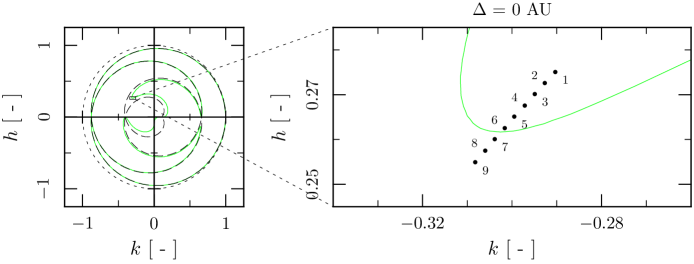
Figure 1: The left-hand side plot depicts in the $kh$ plane ($k$ $=$ $e\cos\sigma$ and $h$ $=$ $e\sin\sigma$) the solutions of resonant condition in the planar circular restricted Sun-Earth-dust problem with solar radiation (green solid line) for a particle with $R$ $=$ 10 $\mu$m, $\varrho$ $=$ 2 g.cm^-3, and $\bar{Q}^{\prime}_{\text{pr}}$ $=$ 1 in the exterior mean motion 6/5 orbital resonance obtained for zero shift. Collisions of the planet and the particle can occur during the synodic period in the shown locations (black dashed line). The right-hand side plot shows locations of initial $kh$ points belonging to evolutions depicted in Figs. 2 and 4 (circles).

The averaged phase space reduced to the eccentricity and the resonant angular variable is depicted in the left-hand side plot of Fig. 1 as the $kh$ plane. The green solid line in Fig. 1 shows numerical solutions of the resonant condition at the shift equal to zero for a particle with $R$ $=$ 10 $\mu$m, $\varrho$ $=$ 2 g.cm^-3, and $\bar{Q}^{\prime}_{\text{pr}}$ $=$ 1 in the exterior mean motion 6/5 orbital resonance with the Earth. The purpose of the left-hand side plot in Fig. 1 is to show locations where the captures into the resonance are possible. The shift zero is used here in order to show later how a non-zero shift influences the solutions of resonant condition. In the $kh$ plane the collisions of the planet with the particle occur on the black dashed curve in Fig. 1. The dashed curves cannot be crossed by the $kh$ point during the evolution in a mean motion resonance. The black rectangle in the left-hand side plot of Fig. 1 contains initial $kh$ points for the evolutions depicted in Figs. 2 and 4. The initial $kh$ points are in the averaged phase space calculated using evolving $e$ and $\sigma$ averaged over the first synodic period of the corresponding evolutions.

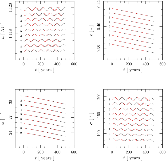
Figure 2: Evolutions of the semimajor axis, eccentricity, longitude of perihelion, and resonant angular variable averaged over the synodic period in the planar circular restricted Sun-Earth-dust problem with the solar radiation. A dust particle with $R$ $=$ 10 $\mu$m, $\varrho$ $=$ 2 g.cm^-3, and $\bar{Q}^{\prime}_{\text{pr}}$ $=$ 1 is initially located in the exterior mean motion 6/5 resonance. The numerical solutions of equation of motion (Eq. 4.1, black solid line) are compared with the linearization solutions (Eq. 132, red dashed line). The evolutions starting with various $\tilde{\omega}$ and $\sigma$ (see text) are successively translated by 4 $\times$ 10^-4 AU, 4 $\times$ 10^-3, 1^∘, and 14^∘ in $a$, $e$, $\tilde{\omega}$ and $\sigma$, respectively. The evolution with the number of initial averaged conditions 5 is not translated.

Figure 3: The numerical solution with the number 5 from Fig. 2 integrated over an interval 8 $\times$ 10⁴ years (black solid line). The interval ends with an asymptotic approach of the eccentricity librations to the universal eccentricity. The horizontal line in the eccentricity plot depicts the universal eccentricity calculated from Eq. (146) for the exterior 6/5 resonance $e_{\text{u}}$ $\approx$ 0.2472 (black dashed line).

A comparison of the numerical (Eq. 4.1, black solid line) and the analytical (Eq. 132, red dashed line) solution is depicted in Fig. 2. Initial conditions for oscular parameters are $\Delta_{\text{in}}$ $=$ 0 AU, $e_{\text{in}}$ $=$ 0.4, $\tilde{\omega}$ $=$ $-$ $\sigma_{\text{in}}$ $q/(p+q)$, and $\sigma_{\text{in}}$ $\in$ $\{136^{\circ},136.5^{\circ},137^{\circ},...,140^{\circ}\}$. Initial true anomalies of the planet and the particle were zero. The curves for $a$, $e$, $\tilde{\omega}$ and $\sigma$ obtained using the various initial conditions are successive translated by 4 $\times$ 10^-4 AU, 4 $\times$ 10^-3, 1^∘, and 14^∘, respectively. Zero translation is at the evolution with the number of initial averaged conditions 5. Without the translation the evolutions of $a$, $e$, and $\sigma$ would be overlapped. The evolutions of $\tilde{\omega}$ without the translation would be shown in the opposite order with a small separation.

The variations of the frequency and the libration amplitude with the initial conditions can be easily seen in the evolutions of the semimajor axis and the resonant angular variable. The evolution of eccentricity is determined by the second equation in Eqs. (2). By solving the condition $de/dt$ $=$ 0 at the solution of resonant condition ($da/dt$ $=$ 0) we obtain the so called “universal eccentricity” (Beaugé & Ferraz-Mello, 1994). The universal eccentricity in the PCRTBP with radiation exists only for the exterior resonances. For the universal eccentricity ($e_{\text{u}}$) holds

$$1-\frac{3e_{\text{u}}^{2}+2}{2\left(1-e_{\text{u}}^{2}\right)^{3/2}}\frac{p+q}{p}=0~{}.$$ (146)

The universal eccentricity in the exterior resonance (given by the resonant numbers $p$ and $q$) is equal for all particles. By the averaging of the second equation in Eqs. (2) over the libration period one obtains governing differential equation for the evolution of eccentricity (Liou & Zook, 1997). The disturbing function in the equation can be hidden using identity $da/dt$ $=$ 0 that is valid for the resonances after the averaging over the libration period. The solution of the condition $de/dt$ $=$ 0 for the exterior resonances is the universal eccentricity. Hence, the eccentricity is constant at the universal eccentricity after the averaging over the libration period. If the initial eccentricity averaged over the libration period is not equal to the universal eccentricity, then the eccentricity in the exterior resonances asymptotically approaches the universal eccentricity. For the exterior 6/5 resonance $e_{\text{u}}$ $\approx$ 0.2472 and the evolutions of eccentricity in Fig. 2 decrease to this value. But the asymptotic value is yet distant from the eccentricities in Fig. 2. In order to show the slowed-down approach of the eccentricity to the universal eccentricity for the evolution number 5 from Fig. 2 we integrated the evolution over an interval of 8 $\times$ 10⁴ years in Fig. 3. At the ends of $\tilde{\omega}$ evolutions in Fig. 2 the linearization solution gives systematically smaller $\tilde{\omega}$ than the solution of the equation of motion. These differences were found to be dependent on $\tilde{\omega}$ used in the averaging of the terms with the disturbing function. For a different $\tilde{\omega}$ giving the same $\sigma$ (see Fig. 6 in Pástor, 2016) the linearization solution can give also slightly larger $\tilde{\omega}$ at the ends of the evolutions. Therefore, this should be numerical feature since in the reality the dependence on $\tilde{\omega}$ should not exists. The libration of $\sigma$ occurs close to $\sigma$ satisfying the resonant condition (Eq. 145).

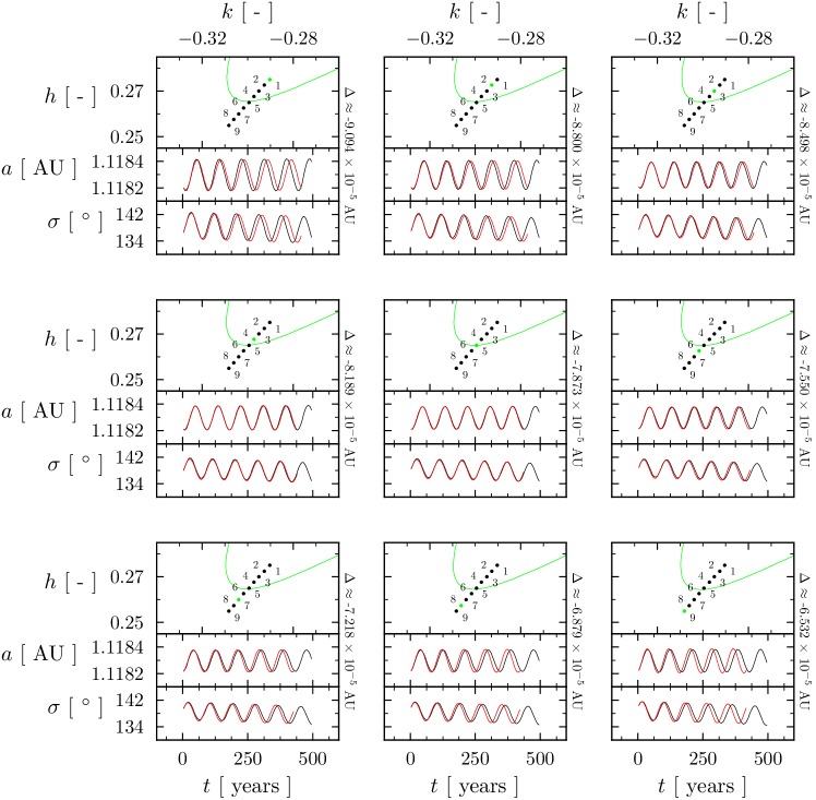
Figure 4: The $kh$ points calculated from the initial averaged $e$ and $\sigma$ of the evolutions in Fig. 2 are shown in the top panel of each plot (circles). The green $kh$ point marks the evolution with the initial shift in the averaged phase space ($\Delta$) written on the right-hand side of plot. The solutions of resonant condition (green solid lines) are obtained for the initial averaged shift. The evolutions of semimajor axis obtained numerically (black solid line) and analytically (red solid line) are compared in the middle panel of each plot. The bottom panels show the compared evolutions of the resonant angular variable.

Main purpose of nine plots in Fig. 4 is to compare variations of the solutions of resonant condition with the varying initial conditions of the evolutions in Fig. 2 in the averaged phase space. The top panel of each plot shows the part of the $kh$ plane equal to the black rectangle in the left-hand side plot of Fig. 1. The initial $kh$ points calculated using $e$ and $\sigma$ averaged over the first synodic period are also shown (circles). The green circle denotes the $kh$ point of the evolution that has the initial averaged shift shown on the right-hand side of each plot. In the averaged phase space the shift differs from the initial shift (zero) used in the un-averaged phase space. The differences exist also for the eccentricity and the resonant angular variable. The shown part of the $kh$ plane depicts the eccentricities and the resonant angular variables satisfying the resonant condition at the initial averaged shift (green solid line). The variations of the positions of green solid lines due to the varying initial averaged shift are smaller than the variations of the initial $kh$ points. This can be seen in Fig. 4 if we compare the solutions of resonant condition at the evolutions 1 and 9. The green solid line at the evolution 1 is between the $kh$ points 4 and 5 and at the evolution 9 is between the $kh$ points 5 and 6. The green solid line obtained at the zero shift in the right-hand side plot of Fig. 1 is between the $kh$ points 6 and 7. It is not easy to hit the solution of resonant condition with the $kh$ point since the averaged values obtained from the numerical solution are discrete.

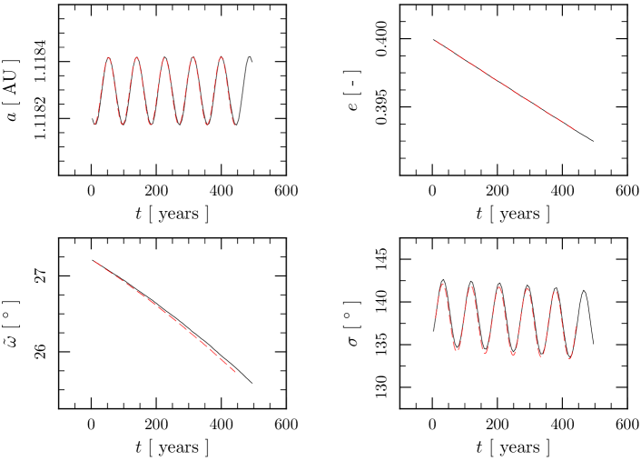
Figure 5: The evolution 1 from Fig. 2 (black solid line) approximated by the linearization solution determined in the averaged phase space with orbital parameters from the first minimum of the semimajor axis (red dashed line).

The middle panel of Fig. 4 shows compared evolutions of the semimajor axis obtained numerically (black solid line) and analytically (red solid line) that are shown and numbered also in Fig. 2. Similarly the bottom panel shows the compared evolutions of the resonant angular variable. The best frequency accordance between the analytical and the numerical solution is found at the evolution 5. The initial conditions in the averaged phase space of the evolution 5 are closest to the solution of the resonant condition at the used initial averaged shift (see Fig. 4). In some cases (mentioned later) the initial conditions closest to the solution of the resonant condition do not give the best accordance between the analytical and the numerical solution. But the best accordance is usually found for the initial conditions not far from this solution.

The property that the best frequency accordance is found at the solution of resonant condition is caused by the evolution of the resonant angular variable. The frequency calculated from the linearization solution in the considered problem most sensitively depends on the initial averaged value of $\sigma$. The dependencies on other initial averaged orbital parameters are much smaller. The linearization frequency is determined in such a way that the evolution of the resonant angular variable is best approximated during a short time interval after the initial time. The found linearization frequency does not have to describe the real libration frequency but the evolutions of orbital parameters have to be correctly described during a sort time interval after the initial time. The linearization frequency significantly varies during librations of $\sigma$ in Fig. 2.

At the solution of resonant condition the averaged time derivative of the semimajor axis is zero. For the resonant angular variable we have

$$\sigma=\frac{p+q}{q}\lambda_{\text{P}}-s\lambda-\tilde{\omega}=\left(\frac{p+q}{q}n_{\text{P}}-sn\right)t+\frac{p+q}{q}\lambda_{\text{P}0}-s(\sigma_{\text{b}}+\tilde{\omega})-\tilde{\omega}~{}.$$ (147)

$n$, $\sigma_{\text{b}}$, and $\tilde{\omega}$ are constant and $\sigma$ depends linearly on time in Keplerian approximation of the motion during the synodic period. When $da/dt$ $=$ 0 in the numerically averaged evolution, then the shift from the exact resonance is minimal or maximal. In the considered approximation the linear time dependence of $\sigma$ is steepest at the solution of resonant condition. The solution of resonant condition is approximately in the middle of $\sigma$ libration. The resonant libration frequency is more accurately determined using the linearization solution when the initial averaged conditions are closer to the solution of resonant condition. The entire evolution during more librations is in this case sufficiently well approximated.

Even for the evolution 1 in Fig. 2 we can obtain an usable linearization solution if we use the initial averaged conditions from later time that are close to the solution of resonant condition for the calculation of the parameters of linearization solution. In other words, the initial averaged conditions close to the minimum or maximum of the semimajor axis. The numerical integration can also start with positions and velocities from later time that are close to the minimum or maximum of the semimajor axis in order to obtain the usable initial averaged conditions in the first synodic period. Such a case is depicted in Fig. 5. However, we must note that the real increase of the semimajor axis during the first libration in Fig. 5 is faster then the increase predicted by the linearization solution and the decrease is slower. This holds also for the evolution 5 in Fig. 2.

Figs. 2, 4, and 5 show the applicability of the linearization solution for the exterior 6/5 resonance with the Earth at the vicinity of one $\sigma$ satisfying the resonant condition at the eccentricity 0.4. The applicability of the linearization solution was checked for various exterior resonances at the vicinity of $\sigma$ satisfying the resonant condition for the eccentricities up to $\sim$0.6.

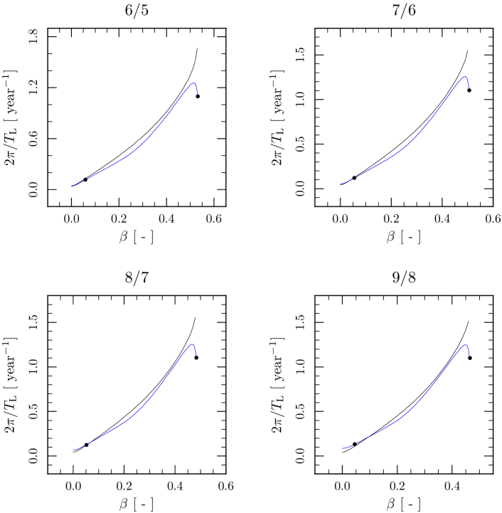
Figure 6: Angular frequencies of the libration for dust particles with various $\beta$ after an infinitesimal displacement from the periodic solutions calculated for 6/5, 7/6, 8/7, and 9/8 exterior resonances in the planar circular restricted Sun-Earth-dust problem with the PR effect and the radial solar wind. The same color in the plots denotes the sets of the periodic solutions emerging from the same $\sigma$ as $\beta$ increases from zero. Circles depict the frequencies of libration for the periodic solutions in the exact resonances (Pástor, 2016).

The resonant angular variable is commonly determined using the initial conditions from the un-averaged phase space with the zero shift. The linearization frequency found for the evolution starting with these initial parameters can be different from the real libration frequency of the evolution. Main reason is the fact that the evolution starting with zero shift in the un-averaged phase space usually does not start at the minimal or maximal semimajor axis in the averaged phase space (in the solution of resonant condition). Although the zero initial shift in the un-averaged phase space usually gives the evolution with a non-zero initial shift in the averaged phase space.

The statements in the previous paragraph can be easily verified if we compare the right-hand side plot in Figs. 1 with the plots in Fig. 4. The best frequency accordance is obtained for the evolution 5 that has the non-zero initial shift from the exact resonance in the averaged phase space. The resonant angular variable obtained from the solution of resonant condition at the zero shift in the right-hand side plot of Fig. 1 is between the initial averaged conditions of the evolutions 6 and 7. The linearization frequency found for $a$ and $e$ from the un-averaged phase space and this $\sigma$ would be between the linearization frequencies found for the evolutions 6 and 7. The evolutions 6 and 7 in Fig. 4 have the zero initial shift in the un-averaged phase space and do not give the best frequency accordance.

The parameters giving the linearization solution for the evolution 5 in Fig. 2 are shown in Appendix D (Table 1). Since the real parts of $\lambda_{1}$ and $\lambda_{3}$ in Table 1 are positive the libration amplitude of the linearization solution increases. This is usually interpreted as an instability. The capture with the non-zero libration amplitude in the PCRTBP with radiation is only temporary. The non-zero libration amplitude increases in accordance with the results valid for the PR effect in Gomes (1995).

4.5 Periodic solutions

For the exterior resonances in the PCRTBP with radiation periodic solutions exist. These periodic solutions set maximal capture time in the exterior resonances theoretically to infinity. Their position in $ae\sigma$ phase space can be obtained as points where $a$, $e$, and $\sigma$ are constant after the averaging over the synodic period for a particle with given $\beta$ (Pástor, 2016). The periodic solutions exist at the universal eccentricity. The libration amplitude of the periodical solutions is zero (Pástor, 2016). Using analytical theory from Gomes (1995) can be proved that the zero libration amplitude does not increase in contrary to the cases with the non-zero libration amplitude. From a theoretical point of view the libration is consistent with a “libration” of a pendulum in an equilibrium point. The frequency of libration can be defined also for these periodic solutions as a frequency of the libration after an infinitesimal displacement from the periodic solution. Such frequencies are calculated in Fig. 6 for the periodic solutions in 6/5, 7/6, 8/7, and 9/8 exterior resonances with the Earth in a circular orbit around radiating Sun. Since the periodic solutions exist at the solution of resonant condition ($da/dt$ $=$ 0) the frequencies are correctly determined from the linearization theory. For periodic solutions the linearization solution does not give exactly the zero libration amplitude, but the obtained libration amplitude is very small.

In the conservative PCRTBP the periodic solutions in the mean motion resonances exist at various eccentricities. These periodic solutions can be obtained using the method in Pástor (2016) without the condition giving the universal eccentricity. Periodic solutions in the circular-planar, spatial-circular, elliptic-planar and spatial-elliptic restricted three-body problem with the PR effect were found to exist for the dust particles captured in the mean motion 1/1 resonance with the planet (Pástor, 2014b; Lhotka & Celletti, 2015).

5 Interstellar gas flow as an example of non-gravitational effect without rotational symmetry

Non-gravitational effects secularly varying orbits in a dependence on their orientation in space are not often considered in the literature. An interstellar gas entering an astrosphere of the star varies the orbits in such a way. The secular variation of orbit in this case depends on the orientation of orbit with respect to an interstellar gas velocity vector. In this section we use secular variations of orbital parameters caused by the stellar radiation and the interstellar gas flow to verify the applicability of the analytical approach derived in Sect. 3.

5.1 Equation of motion

The interstellar matter containing $i$ gas components with temperatures $T_{i}$ moving with a relative velocity $\vec{v_{\text{F}}}$ with respect to the star affects the dynamic of a spherical dust particle according to Baines, Williams & Asebiomo (1965) with the acceleration

$$\frac{d\vec{v}}{dt}=-\sum_{i=1}^{N}c_{\text{D}i}\gamma_{i}|\vec{v}-\vec{v}_{\text{F}}|\left(\vec{v}-\vec{v}_{\text{F}}\right)~{}.$$ (148)

$c_{\text{D}i}$ in Eq. (148) is the drag coefficient

$$c_{\text{D}i}(s_{i})={} \frac{1}{\sqrt{\pi}}\left(\frac{1}{s_{i}}+\frac{1}{2s_{i}^{3}}\right)\text{e}^{-s_{i}^{2}}+\left(1+\frac{1}{s_{i}^{2}}-\frac{1}{4s_{i}^{4}}\right)\text{erf}(s_{i})$$

$$+\left(1-\delta_{i}\right)\left(\frac{T_{\text{d}}}{T_{i}}\right)^{1/2}\frac{\sqrt{\pi}}{3s_{i}}~{},$$ (149)

where erf$(s_{i})$ is the error function $\text{erf}(s_{i})$ $=$ $2/\sqrt{\pi}\int_{0}^{s_{i}}\text{e}^{-t_{\text{p}}^{2}}dt_{\text{p}}$, $\delta_{i}$ is the fraction of impinging particles specularly reflected at the surface (a diffuse reflection is assumed for the rest of the particles, see Baines, Williams & Asebiomo 1965; Gustafson 1994), $T_{\text{d}}$ is the temperature of the dust grain. $s_{i}$ in Eq. (5.1) is the molecular speed ratio

$$s_{i}=\sqrt{\frac{m_{i}}{2kT_{i}}}U~{}.$$ (150)

Here $m_{i}$ is the mass of the atom in the $i$th gas component, $k$ is Boltzmann’s constant, and $U$ $=$ $|\vec{v}-\vec{v}_{\text{F}}|$ is the relative speed of the dust particle with respect to the gas. For the collision parameter $\gamma_{i}$ in Eq. (148) we find

$$\gamma_{i}=n_{i}\frac{m_{i}}{m}A^{\prime}~{},$$ (151)

where $n_{i}$ is the number density of the $i$th gas component, and $A^{\prime}$ is the geometrical cross section of the dust grain.

The interstellar wind enters the Solar system with relative velocity 26.3 km/s and comes from the direction $\lambda_{\text{ecl}}$ $=$ 254.7^∘ (heliocentric ecliptic longitude) and $\beta_{\text{ecl}}$ $=$ 5.2^∘ (heliocentric ecliptic latitude; Lallement et al. 2005). After the passage through various layers caused by magnetohydrodynamic interaction of the interstellar wind with the solar wind the original interstellar hydrogen that remains unaffected has the number density $n_{\text{H~{}I}}$ $=$ 0.059 g.cm^-3 (Frisch et al., 2009). The interstellar helium reaches inner Solar system (neighborhood of the Earth’s orbit) weakly affected by the interaction with the density $n_{\text{He}}$ $=$ 0.015 g.cm^-3 and the temperature $T_{\text{He}}$ $=$ 6300 K (Frisch et al., 2009). The temperature of the interstellar helium moving freely to the inner Solar system is approximately equal to the temperature of the unaffected interstellar wind. The original interstellar hydrogen produces the so-called second population by the charge exchange with protons in the outer heliosheath (between the bowshock and the heliopause). We used the density $n_{\text{H~{}II}}$ $=$ 0.059 g.cm^-3 for the second population of the interstellar hydrogen after the passage into the heliosphere (Frisch et al., 2009). The temperatures of two hydrogen populations are different due to the charge exchange. We used $T_{\text{H~{}I}}$ $=$ 6100 K and $T_{\text{H~{}II}}$ $=$ 16500 K (Frisch et al., 2009).

When we add the acceleration in Eq. (148) to Eq. (4.1), then we obtain the final equation of motion of the dust grain in the PCRTBP with the stellar radiation and the interstellar gas flow

$$\frac{d\vec{v}}{dt}={} -\frac{\mu}{r^{2}}\left(1-\beta\right)\vec{e}_{\text{R}}-\frac{G_{0}M_{\text{P}}}{|\vec{r}-\vec{r}_{\text{P}}|^{3}}(\vec{r}-\vec{r}_{\text{P}})-\frac{G_{0}M_{\text{P}}}{r_{\text{P}}^{3}}\vec{r}_{\text{P}}$$

$$-\beta\frac{\mu}{r^{2}}\left(1+\frac{\eta}{\bar{Q}^{\prime}_{\text{pr}}}\right)\left(\frac{\vec{v}\cdot\vec{e}_{\text{R}}}{c}\vec{e}_{\text{R}}+\frac{\vec{v}}{c}\right)$$

$$-\sum_{i=1}^{N}c_{\text{D}i}\gamma_{i}|\vec{v}-\vec{v}_{\text{F}}|\left(\vec{v}-\vec{v}_{\text{F}}\right)~{}.$$ (152)

5.2 Secular variations

An expansion of the particle’s acceleration in Eq. (148) using Taylor series enables the calculation of secular time derivatives of the orbital parameters from Gauss’s perturbation equations (Pástor, 2012b, 2014a). The calculated secular time derivatives of orbital parameters for the stellar radiation and the interstellar gas flow are

$$\left(\frac{da}{dt}\right)_{\text{EF}}={} -\frac{\beta\mu}{ca\alpha^{3}}\left(1+\frac{\eta}{\bar{Q}^{\prime}_{\text{pr}}}\right)\left(2+3e^{2}\right)$$

$$-\sum_{i=1}^{N}\frac{2c_{0i}\gamma_{i}v_{\text{F}}^{2}\sigma_{\text{F}}a^{2}\alpha}{L}\left[1+\frac{g_{i}\left(S^{2}+\alpha I^{2}\right)}{v_{\text{F}}^{2}\left(1+\alpha\right)}\right]~{},$$

$$\left(\frac{de}{dt}\right)_{\text{EF}}={} -\frac{\beta\mu}{2ca^{2}\alpha}\left(1+\frac{\eta}{\bar{Q}^{\prime}_{\text{pr}}}\right)5e$$

$$+\sum_{i=1}^{N}\frac{c_{0i}\gamma_{i}v_{\text{F}}a\alpha}{2L}\left[3I+\frac{\sigma_{\text{F}}g_{i}\alpha^{2}\left(1-\alpha\right)\left(I^{2}-S^{2}\right)}{v_{\text{F}}e\left(1+\alpha\right)}\right]~{},$$

$$\left(\frac{d\tilde{\omega}}{dt}\right)_{\text{EF}}={} \sum_{i=1}^{N}\frac{c_{0i}\gamma_{i}v_{\text{F}}a\alpha S}{2L}\left\{-\frac{3}{e}+\frac{\sigma_{\text{F}}g_{i}I}{v_{\text{F}}}\left[\frac{2\alpha^{2}}{\left(1+\alpha\right)^{2}}-1\right]\right\}~{},$$

$$\left(\frac{d\sigma_{\text{b}}}{dt}+t\frac{dn}{dt}\right)_{\text{EF}}={} \sum_{i=1}^{N}\frac{c_{0i}\gamma_{i}v_{\text{F}}aS}{2L}\Biggl{\{}\frac{3\left(1+e^{2}\right)}{e}-\frac{\sigma_{\text{F}}g_{i}\alpha^{2}I}{v_{\text{F}}}$$

$$\times\left[\frac{2\alpha^{2}}{\left(1+\alpha\right)^{2}}-1\right]\Biggr{\}}~{}.$$ (153)

Here

$$S =v_{\text{F}x}\cos\tilde{\omega}+v_{\text{F}y}\sin\tilde{\omega}~{},$$

$$I =-v_{\text{F}x}\sin\tilde{\omega}+v_{\text{F}y}\cos\tilde{\omega}~{}.$$ (154)

with $v_{\text{F}x}$ and $v_{\text{F}y}$ denoting the Cartesian components of the interstellar gas flow velocity vector.

$$\sigma_{\text{F}}=\frac{1}{v_{\text{F}}}\sqrt{\frac{\mu(1-\beta)}{a(1-e^{2})}}~{}.$$ (155)

Only the orbits with $\sigma_{\text{F}}^{2}$ negligible in a comparison with $\sigma_{\text{F}}$ are considered in the expansion. $c_{0i}$ are the drag coefficients for the dust particle at the rest with respect to the star. The parameters $g_{i}$ describe dependences of the drag coefficients on the velocity of dust particle with respect to the star. For constant drag coefficients hold $g_{i}$ $=$ 1 (Pástor, 2012b). Some of Eqs. (5.2) are singular in the eccentricity due to the reasons mentioned after Eqs. (2).

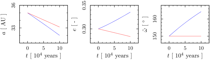
Figure 7: A comparison of secular evolutions obtained before (red solid line) and after (blue solid line) the addition of the interstellar gas flow to the solar radiation acting on a dust particle with $R$ $=$ 2 $\mu$m, $\varrho$ $=$ 1 g.cm^-3, and $\bar{Q}^{\prime}_{\text{pr}}$ $=$ 1. The evolutions of the semimajor axis, eccentricity, and longitude of perihelion are averaged over the orbital period. The secular evolutions are significantly influenced by the interstellar gas flow at the heliocentric distances where a capture into the mean motion resonance with the Neptune can occur.

For the dust particles in the inner Solar system the acceleration from the interstellar gas flow can be neglected in comparison with the accelerations from the PR effect and the solar wind. However, in the vicinity of Neptune’s orbit the acceleration from the interstellar gas flow dominates in the secular evolution of the dust particles. Variations in the particle’s secular evolution caused by the addition of the interstellar gas flow to the solar radiation are illustrated in Fig. 7. In these plots a dust particle with $R$ $=$ 2 $\mu$m, $\varrho$ $=$ 1 g.cm^-3, and $\bar{Q}^{\prime}_{\text{pr}}$ $=$ 1 evolves from the initial conditions $a_{\text{in}}$ $=$ 35 AU, $e_{\text{in}}$ $=$ 0.3, $\tilde{\omega}$ $=$ 150^∘, and $f_{\text{in}}$ $=$ 180^∘ without the gravitational influence of the planet. The dependence of the drag coefficients on the velocity of dust particle with respect to the star is considered (Eq. 5.1). As can be seen in Fig. 7 the influence of the interstellar gas flow cannot be neglected in the vicinity of Neptune’s orbit. On the bound orbits the addition of the interstellar gas flow causes always faster decrease of the semimajor axis, the eccentricity can also increase (instead of the monotonic decrease caused by the solar radiation), and the longitude of perihelion is not constant (compare Eqs. 4.2 and Eqs. 5.2).

Inclination between the Neptune’s orbital plane and the interstellar gas velocity vector is 3.7^∘. Therefore, the assumption that the solved problem is planar is not strictly correct. The secular time derivative of the inclination caused by the interstellar gas flow is for orbits with $i$ $\approx$ 0 proportional to $v_{\text{F}z}$ (Pástor, 2012b) and this velocity component is small in coordinates with the $xy$ plane lying in the Neptune’s orbital plane. Hence, the inclination can be well approximated by a constant value close to zero. This is also confirmed by the numerical integration of the equation of motion. In order to obtain results for the PCRTBP with the PR effect, solar wind and interstellar gas flow we rotated the interstellar gas velocity vector into the Neptune’s orbital plane around an axis perpendicular to the interstellar gas velocity vector and lying in the Neptune’s orbital plane.

5.3 Linearization of averaged resonant equations

The partial derivatives with respect to $a$, $e$, $\tilde{\omega}$, and $\sigma$ can be calculated using Eqs. (5.2) (see Eqs. A in Appendix A). The solved problem does not have the rotational symmetry for the interstellar gas flow and $\Lambda_{0}$ $\neq$ 0. The $\Lambda_{3}$, $\Lambda_{2}$, $\Lambda_{1}$, and $\Lambda_{0}$ calculated from Eqs. (20)-(53) determine $\lambda_{i}$ as roots of the quadric equation Eq. (137).

5.4 Numerical checking

The varying longitude of pericenter affects the secular evolution of dust particles when the interstellar gas is moving through the PCRTBP with radiation. The phase space containing all evolution for a given mean motion resonance in the PCRTBP with radiation and interstellar gas flow has five dimensions ($\beta$, $a$, $e$, $\tilde{\omega}$, $\sigma$). The resonant condition is in this case

$$\frac{da}{dt}={} -\frac{2sa}{L}\frac{\partial R}{\partial\sigma}-\frac{\beta\mu}{ca\alpha^{3}}\left(1+\frac{\eta}{\bar{Q}^{\prime}_{\text{pr}}}\right)\left(2+3e^{2}\right)$$

$$-\sum_{i=1}^{N}\frac{2c_{0i}\gamma_{i}v_{\text{F}}^{2}\sigma_{\text{F}}a^{2}\alpha}{L}\left[1+\frac{g_{i}\left(S^{2}+\alpha I^{2}\right)}{v_{\text{F}}^{2}\left(1+\alpha\right)}\right]=0~{}.$$ (156)

For the sake of simplicity we fixed the semimajor axis in the averaged phase space by using $\Delta$ $=$ 0 and $\beta$ by choosing one dust particle with $R$ $=$ 2 $\mu$m, $\varrho$ $=$ 1 g.cm^-3, and $\bar{Q}^{\prime}_{\text{pr}}$ $=$ 1. We solved the resonant condition for the exact resonance at various longitudes of perihelion in the $kh$ plane. Interesting property was found. The solution of resonant condition does not significantly depend on the longitude of perihelion for the considered dust particle and the interstellar gas in the Solar system. The variations of the resonant angular variable found from the resonant condition at a given eccentricity ($e$ $\apprle$ 1 see further) due to the longitude of perihelion (varying in the interval [0, 2$\pi$]) are typically less than one degree. The variations in the extreme orientations $S$ $=$ $v_{\text{F}}$ and $I$ $=$ $v_{\text{F}}$ were also compared. This property was verified for various resonances with the Neptune and holds also if the Neptune is replaced with the Earth-mass planet. But when the interstellar gas flow is not considered, then the solution of resonant condition is different. The solution of the resonant condition with $\Delta$ $=$ 0 and $\tilde{\omega}$ $=$ 0 for the dust particle with $R$ $=$ 2 $\mu$m, $\varrho$ $=$ 1 g.cm^-3, and $\bar{Q}^{\prime}_{\text{pr}}$ $=$ 1 in the exterior mean motion 3/2 resonance with the Neptune is depicted in Fig. 8. The solutions of resonant condition are close to the collisions for high eccentricities. The high eccentricities are shown only for a completeness of the depicted solutions, since the approximation mentioned below Eq. (155) does not hold well for the eccentricities $\apprge$ 0.8 in the considered problem. The right-hand side panel shows a region containing the initial averaged conditions for Figs. 9 and 10.

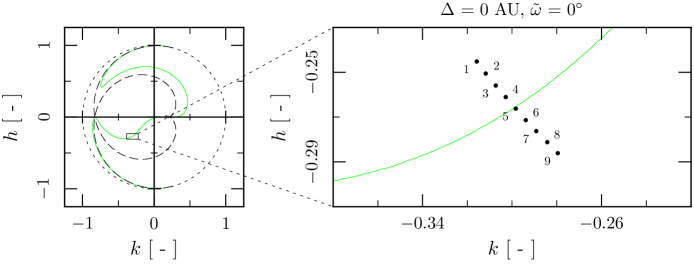
Figure 8: The $kh$ plane containing the solutions of resonant condition in the PCRTBP with solar radiation and interstellar gas flow at the shift $\Delta$ $=$ 0 and the longitude of perihelion $\tilde{\omega}$ $=$ 0 for the dust particle with $R$ $=$ 2 $\mu$m, $\varrho$ $=$ 1 g.cm^-3, and $\bar{Q}^{\prime}_{\text{pr}}$ $=$ 1 in the exterior mean motion 3/2 resonance with the Neptune. The initial averaged conditions belonging to the evolutions depicted in Figs. 9 and 10 are shown in the scaled rectangle region of the $kh$ plane. The same legend as in Fig. 1 is used.

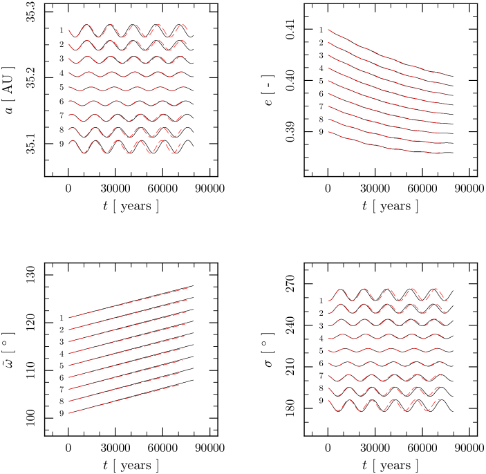
Figure 9: The same plots as in Fig. 2 for the PCRTBP with different planet, particle, resonance, and non-gravitational effects. A dust particle with $R$ $=$ 2 $\mu$m, $\varrho$ $=$ 1 g.cm^-3, and $\bar{Q}^{\prime}_{\text{pr}}$ $=$ 1 is initially located in the exterior mean motion 3/2 resonance with the Neptune under the action of the PR effect, solar wind and interstellar gas flow. The successive translations of evolutions $a$, $e$, $\tilde{\omega}$, and $\sigma$ are 2.2 $\times$ 10^-2 AU, 2.5 $\times$ 10^-3, 3^∘, and 10^∘, respectively. The evolution 5 is not translated.

Fig. 9 shows evolutions of the semimajor axis, eccentricity, longitude of perihelion, and resonant angular variable calculated numerically from the equation of motion (Eq. 5.1) and analytically from Eq. (136) using the initial averaged conditions in Eqs. (A). Initial conditions for oscular parameters are $\Delta_{\text{in}}$ $=$ 0 AU, $e_{\text{in}}$ $=$ 0.4, $\tilde{\omega}$ $=$ $-$ $\sigma_{\text{in}}$ $q/(p+q)$, and $\sigma_{\text{in}}$ $\in$ $\{218^{\circ},219^{\circ},220^{\circ},...,226^{\circ}\}$. The initial true anomalies of the planet and the particle were zero. The successive translations of the obtained curves for $a$, $e$, $\tilde{\omega}$, and $\sigma$ are 2.2 $\times$ 10^-2 AU, 2.5 $\times$ 10^-3, 3^∘, and 10^∘, respectively. The zero translation is at the evolution 5. As in Fig. 2 the evolutions of $\tilde{\omega}$ without the translation would be shown in the opposite order with a small separation and the evolutions of the other orbital parameters would be overlapped. The eccentricity does not approach the universal eccentricity due to the dependence of the secular time derivatives of the semimajor axis and the eccentricity on the longitude of perihelion. The universal eccentricity does not exit for the considered non-gravitational effects (Pástor, 2014a). Oscillations in the evolution of eccentricity can be seen. The eccentricity evolves non-monotonically for the evolutions with the numbers from 7 to 9. During the same number of librations the longitude of perihelion varies more rapidly in Fig. 9 in comparison with Fig. 2.

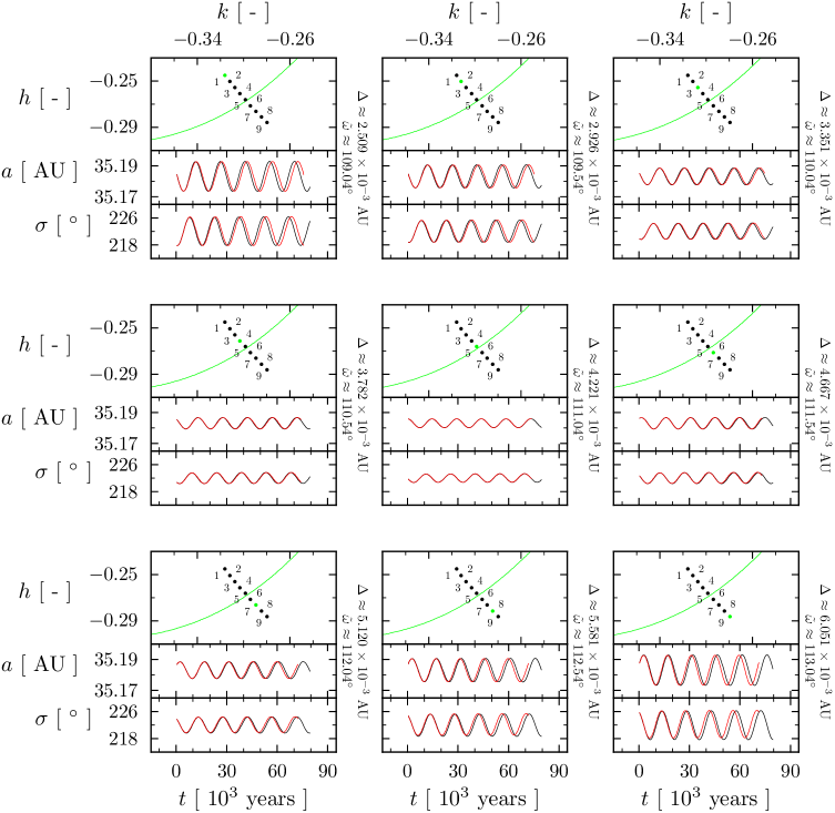
Figure 10: The same plots as in Fig. 4 depicting data from the evolutions in Fig. 9. Each plot in addition to the initial averaged shift contains on the right-hand side also the initial averaged longitude of perihelion at which was the resonant condition solved for the evolution marked with the green $kh$ point.

The linearization frequency well corresponds to the real libration frequency at the solution of resonant condition as can be seen in Fig. 10. The top panel of each plot shows the solution of resonant condition in the $kh$ plane calculated for the initial averaged values of the shift and the longitude of perihelion belonging to the evolution with the green $kh$ point. The librations of the semimajor axis and the resonant angular variable in Fig. 9 are shown with a different scale in two bottom panels of each plot in Fig. 10. The best frequency accordance is obtained at the evolution 5. The green line of this evolution is between the $kh$ points 5 and 6.

The parameters giving the linearization solution for the evolution 5 are shown in Appendix D (Table 2). The libration amplitude increases also for the linearization solution in Table 2 since the real parts of $\lambda_{3}$ and $\lambda_{4}$ are positive and the others roots are real. This analytically indicates an instability for the exterior resonances in the PCRTBP with the solar radiation and interstellar gas flow. The majority of captures end due to the increase of libration amplitude (Pástor, 2013). However, it is possible to find also the evolutions in the exterior resonances with temporary decreasing libration amplitude.

For the resonant evolutions with much larger libration amplitudes of $\sigma$ as those in Figs. 4 and 10 the best frequency accordance is shifted farther from the solution of resonant condition. In these cases the linearization is not good method for the calculation of the libration frequency.

5.5 Periodic solutions

In the PCRTBP with solar radiation and interstellar gas flow such periodic solutions as those in Sect. 4.5 have not been found. If such periodic solutions exist, then they must have a fixed (constant) longitude of perihelion in the averaged phase space. Existence of these periodic orbits is unlikely (Pástor, 2014a). In general, the condition for the fixed longitude of pericenter depends on the nature of the non-gravitational effects. As a special case can theoretically exist the non-gravitational effects without the rotational symmetry that have periodic solutions with the varying longitude of pericenter. However, also for such non-gravitational effects the condition for the fixed longitude of pericenter could give a different set of the periodic orbits.

6 Conclusion

We have derived the averaged resonant equations in the PCRTBP with the non-gravitational effects using summed Lagrange’s planetary equations and Gauss’s perturbation equations in few simple steps. The averaged resonant equations were linearized and solved for the standard solution in a general form. The planarity of problem restricts maximal number of evolving parameters describing the orbit to four. For four evolving parameters the degree of the characteristic polynomial is four and its analytical solution always exists. This would not be case for a higher number of evolving parameters. For problems that include the non-gravitational effects acting with the rotational symmetry around the star the longitude of pericenter evolves separately and does not affect remaining three parameters. The applicability of the linearization solution does not significantly depend on the variations of the orbit during the averaged synodic period. This confirms that the evolutions in the mean motion resonances can be correctly described by the averaged resonant equations. The actual positions of the planet and the dust particle in the space are not important for the correct secular evolution.

The linearization frequency depends most sensitively on the initial averaged value of the resonant angular variable in the comparison with dependences on the initial averaged values of the other evolving orbital parameters. The linearization frequency matches best the real libration frequency for such initial averaged conditions that are close to the solution of resonant condition. The solutions of resonant condition are located in the evolution of the semimajor axis in the minima or maxima. The minima or maxima of the semimajor axis occur approximately in the middle of libration in the evolution of the resonant angular variable.

When the libration amplitude of the resonant angular variable is larger, then the best frequency accordance is shifted farther from the solutions of resonant condition. In these cases the validity of linearization solution disappears. The stationary solutions exist at the solutions of resonant condition and the resonant angular variable of the stationary conditions is constant therefore their “frequency” obtained from the linearization solution should be correct.

The linearization solution can be used as an indicator of the stability of the resonant captures. For example when a small libration amplitude of the linearization solution always decreases, then the capture time should be theoretically be infinitely long. However, when for a stationary solution the linearization solution gives an increase of the libration amplitude, then this not necessarily means that the capture time of the stationary solution is theoretically finite. As an example we can mention the periodic solutions for the exterior resonances in the PCRTBP with stellar radiation (Sect. 4.5). In this case a small displacement of the initial conditions from the stationary solution causes the increase of libration amplitude. The increase of libration amplitude is proportional to the libration amplitude and this implies that the zero libration amplitude does not increase. Therefore, it is practically impossible to choose finite numerical values of the initial conditions for the linearization solution that should give the constant zero libration amplitude of the stationary solution. In this case the linearization solution always gives a small increase of the libration amplitude regardless of numerical limits of averaging in order to obtain the zero time derivatives of the orbital parameters.

In the PCRTBP with the PR effect, radial solar wind, and interstellar gas flow the resonant angular variable satisfying the resonant condition at a given eccentricity insignificantly depend on the longitude of perihelion (compare Fig. 8 and Fig. 10). For the exterior resonances in this asymmetrical problem the libration amplitude of the real evolution usually increases, but the resonant captures with temporary decreasing libration amplitude exist also.

Appendix A Constant coefficients

This appendix presents coefficients for linearized system of equations describing the orbital evolutions of the dust particles captured in the mean motion resonances in the PCRTBP with the PR effect, radial stellar wind and interstellar gas flow (Eqs. 3).

$$A_{\text{c}}={} -\frac{s}{L_{0}}\frac{\partial R}{\partial\sigma}-\frac{2sa_{0}}{L_{0}}\frac{\partial^{2}R}{\partial^{\star}a\partial\sigma}+\frac{\beta\mu}{ca_{0}^{2}\alpha_{0}^{3}}\left(1+\frac{\eta}{\bar{Q}^{\prime}_{\text{pr}}}\right)\left(2+3e_{0}^{2}\right)$$

$$-\sum_{i=1}^{N}\frac{2c_{0i}\gamma_{i}v_{\text{F}}^{2}\sigma_{\text{F}}a_{0}\alpha_{0}}{L_{0}}\left[1+\frac{g_{i}\left(S_{0}^{2}+\alpha_{0}I_{0}^{2}\right)}{v_{\text{F}}^{2}\left(1+\alpha_{0}\right)}\right]~{},$$

$$B_{\text{c}}={} -\frac{2sa_{0}}{L_{0}}\frac{\partial^{2}R}{\partial e\partial\sigma}-\frac{3\beta\mu e_{0}}{ca_{0}\alpha_{0}^{5}}\left(1+\frac{\eta}{\bar{Q}^{\prime}_{\text{pr}}}\right)\left(4+e_{0}^{2}\right)-\sum_{i=1}^{N}\frac{2c_{0i}\gamma_{i}\sigma_{\text{F}}a_{0}^{2}e_{0}}{L_{0}}\frac{g_{i}\left(S_{0}^{2}-I_{0}^{2}\right)}{\left(1+\alpha_{0}\right)^{2}}~{},$$

$$C_{\text{c}}={} -\sum_{i=1}^{N}\frac{4c_{0i}\gamma_{i}\sigma_{\text{F}}a_{0}^{2}\alpha_{0}}{L_{0}}\frac{g_{i}S_{0}I_{0}\left(1-\alpha_{0}\right)}{1+\alpha_{0}}~{},$$

$$D_{\text{c}}={} -\frac{2sa_{0}}{L_{0}}\frac{\partial^{2}R}{\partial\sigma^{2}}~{},$$

$$E_{\text{c}}={} 0~{},$$

$$F_{\text{c}}={} -\frac{2sa_{0}}{L_{0}}\frac{\partial R}{\partial\sigma}-\frac{\beta\mu}{ca_{0}\alpha_{0}^{3}}\left(1+\frac{\eta}{\bar{Q}^{\prime}_{\text{pr}}}\right)\left(2+3e_{0}^{2}\right)$$

$$-\sum_{i=1}^{N}\frac{2c_{0i}\gamma_{i}v_{\text{F}}^{2}\sigma_{\text{F}}a_{0}^{2}\alpha_{0}}{L_{0}}\left[1+\frac{g_{i}\left(S_{0}^{2}+\alpha_{0}I_{0}^{2}\right)}{v_{\text{F}}^{2}\left(1+\alpha_{0}\right)}\right]~{},$$

$$G_{\text{c}}={} -\frac{\alpha_{0}}{2a_{0}L_{0}e_{0}}\left[1+s\left(1-\alpha_{0}\right)\right]\frac{\partial R}{\partial\sigma}+\frac{\alpha_{0}}{L_{0}e_{0}}\left[1+s\left(1-\alpha_{0}\right)\right]\frac{\partial^{2}R}{\partial^{\star}a\partial\sigma}$$

$$+\frac{\beta\mu}{ca_{0}^{3}\alpha_{0}}\left(1+\frac{\eta}{\bar{Q}^{\prime}_{\text{pr}}}\right)5e_{0}+\sum_{i=1}^{N}\frac{3c_{0i}\gamma_{i}v_{\text{F}}\alpha_{0}I_{0}}{4L_{0}}~{},$$

$$H_{\text{c}}={} -\frac{1}{L_{0}e_{0}^{2}\alpha_{0}}\left[1+s\left(1-\alpha_{0}\right)\right]\frac{\partial R}{\partial\sigma}+\frac{s}{L_{0}}\frac{\partial R}{\partial\sigma}+\frac{\alpha_{0}}{L_{0}e_{0}}\left[1+s\left(1-\alpha_{0}\right)\right]\frac{\partial^{2}R}{\partial e\partial\sigma}$$

$$-\frac{5\beta\mu}{2ca_{0}^{2}\alpha_{0}^{3}}\left(1+\frac{\eta}{\bar{Q}^{\prime}_{\text{pr}}}\right)$$

$$-\sum_{i=1}^{N}\frac{c_{0i}\gamma_{i}v_{\text{F}}^{2}a_{0}}{2L_{0}}\left\{\frac{3e_{0}I_{0}}{v_{\text{F}}\alpha_{0}}+\frac{\sigma_{\text{F}}g_{i}\alpha_{0}}{v_{\text{F}}^{2}}\left[1-\frac{3}{\left(1+\alpha_{0}\right)^{2}}\right]\left(S_{0}^{2}-I_{0}^{2}\right)\right\}~{},$$

$$I_{\text{c}}={} -\sum_{i=1}^{N}\frac{c_{0i}\gamma_{i}v_{\text{F}}^{2}a_{0}\alpha_{0}}{L_{0}}\left[\frac{3S_{0}}{2v_{\text{F}}}+\frac{2\sigma_{\text{F}}g_{i}\alpha_{0}^{2}\left(1-\alpha_{0}\right)S_{0}I_{0}}{v_{\text{F}}^{2}e_{0}\left(1+\alpha_{0}\right)}\right]~{},$$

$$J_{\text{c}}={} \frac{\alpha_{0}}{L_{0}e_{0}}\left[1+s\left(1-\alpha_{0}\right)\right]\frac{\partial^{2}R}{\partial\sigma^{2}}~{},$$

$$K_{\text{c}}={} 0~{},$$

$$L_{\text{c}}={} \frac{\alpha_{0}}{L_{0}e_{0}}\left[1+s\left(1-\alpha_{0}\right)\right]\frac{\partial R}{\partial\sigma}-\frac{5\beta\mu}{2ca_{0}^{2}\alpha_{0}}\left(1+\frac{\eta}{\bar{Q}^{\prime}_{\text{pr}}}\right)e_{0}$$

$$+\sum_{i=1}^{N}\frac{c_{0i}\gamma_{i}v_{\text{F}}^{2}a_{0}\alpha_{0}}{2L_{0}}\left[\frac{3I_{0}}{v_{\text{F}}}-\frac{\sigma_{\text{F}}g_{i}\alpha_{0}^{2}\left(1-\alpha_{0}\right)\left(S_{0}^{2}-I_{0}^{2}\right)}{v_{\text{F}}^{2}e_{0}\left(1+\alpha_{0}\right)}\right]~{},$$

$$M_{\text{c}}={} -\frac{\alpha_{0}}{2a_{0}L_{0}e_{0}}\frac{\partial R}{\partial e}+\frac{\alpha_{0}}{L_{0}e_{0}}\frac{\partial^{2}R}{\partial^{\star}a\partial e}-\sum_{i=1}^{N}\frac{3c_{0i}\gamma_{i}v_{\text{F}}\alpha_{0}S_{0}}{4L_{0}e_{0}}~{},$$

$$N_{\text{c}}={} -\frac{1}{L_{0}e_{0}^{2}\alpha_{0}}\frac{\partial R}{\partial e}+\frac{\alpha_{0}}{L_{0}e_{0}}\frac{\partial^{2}R}{\partial e^{2}}+\sum_{i=1}^{N}\frac{c_{0i}\gamma_{i}v_{\text{F}}a_{0}S_{0}}{L_{0}}\left[\frac{3}{2e_{0}^{2}\alpha_{0}}-\frac{2\sigma_{\text{F}}g_{i}\alpha_{0}e_{0}I_{0}}{v_{\text{F}}\left(1+\alpha_{0}\right)^{3}}\right]~{},$$

$$O_{\text{c}}={} -\sum_{i=1}^{N}\frac{c_{0i}\gamma_{i}v_{\text{F}}a_{0}\alpha_{0}}{2L_{0}}\left\{\frac{3I_{0}}{e_{0}}+\frac{\sigma_{\text{F}}g_{i}}{v_{\text{F}}}\left[\frac{2\alpha_{0}^{2}}{\left(1+\alpha_{0}\right)^{2}}-1\right]\left(S_{0}^{2}-I_{0}^{2}\right)\right\}~{},$$

$$P_{\text{c}}={} \frac{\alpha_{0}}{L_{0}e_{0}}\frac{\partial^{2}R}{\partial\sigma\partial e}~{},$$

$$Q_{\text{c}}={} 0~{},$$

$$R_{\text{c}}={} \frac{\alpha_{0}}{L_{0}e_{0}}\frac{\partial R}{\partial e}+\sum_{i=1}^{N}\frac{c_{0i}\gamma_{i}v_{\text{F}}a_{0}\alpha_{0}S_{0}}{2L_{0}}\left\{-\frac{3}{e_{0}}+\frac{\sigma_{\text{F}}g_{i}I_{0}}{v_{\text{F}}}\left[\frac{2\alpha_{0}^{2}}{\left(1+\alpha_{0}\right)^{2}}-1\right]\right\}~{},$$

$$S_{\text{c}}={} \frac{\alpha_{0}}{2a_{0}L_{0}e_{0}}\left[1+s\left(1-\alpha_{0}\right)\right]\frac{\partial R}{\partial e}-\frac{\alpha_{0}}{L_{0}e_{0}}\left[1+s\left(1-\alpha_{0}\right)\right]\frac{\partial^{2}R}{\partial^{\star}a\partial e}+\frac{s}{L_{0}}\frac{\partial R}{\partial^{\star}a}+\frac{2sa_{0}}{L_{0}}\frac{\partial^{2}R}{\partial^{\star}a^{2}}$$

$$+\frac{3sn_{0}}{2a_{0}}-s\sum_{i=1}^{N}\frac{3c_{0i}\gamma_{i}v_{\text{F}}e_{0}S_{0}}{2L_{0}}+\left[1+s\left(1-\alpha_{0}\right)\right]\sum_{i=1}^{N}\frac{3c_{0i}\gamma_{i}v_{\text{F}}\alpha_{0}S_{0}}{4L_{0}e_{0}}~{},$$

$$T_{\text{c}}={} \frac{1}{L_{0}e_{0}^{2}\alpha_{0}}\left[1+s\left(1-\alpha_{0}\right)\right]\frac{\partial R}{\partial e}-\frac{\alpha_{0}}{L_{0}e_{0}}\left[1+s\left(1-\alpha_{0}\right)\right]\frac{\partial^{2}R}{\partial e^{2}}-\frac{s}{L_{0}}\frac{\partial R}{\partial e}+\frac{2sa_{0}}{L_{0}}\frac{\partial^{2}R}{\partial e\partial^{\star}a}$$

$$-s\sum_{i=1}^{N}\frac{c_{0i}\gamma_{i}v_{\text{F}}a_{0}S_{0}}{2L_{0}}\left\{3+\frac{\sigma_{\text{F}}g_{i}e_{0}I_{0}}{v_{\text{F}}}\left[\frac{2\alpha_{0}^{2}}{\left(1+\alpha_{0}\right)^{2}}-1\right]\right\}$$

$$+\left[1+s\left(1-\alpha_{0}\right)\right]\sum_{i=1}^{N}\frac{c_{0i}\gamma_{i}v_{\text{F}}a_{0}S_{0}}{L_{0}}\left[-\frac{3}{2e_{0}^{2}\alpha_{0}}+\frac{2\sigma_{\text{F}}g_{i}e_{0}\alpha_{0}I_{0}}{v_{\text{F}}\left(1+\alpha_{0}\right)^{3}}\right]~{},$$

$$U_{\text{c}}={} -s\sum_{i=1}^{N}\frac{3c_{0i}\gamma_{i}v_{\text{F}}a_{0}e_{0}I_{0}}{L_{0}}$$

$$+\left[1+s\left(1-\alpha_{0}\right)\right]\sum_{i=1}^{N}\frac{c_{0i}\gamma_{i}v_{\text{F}}^{2}a_{0}\alpha_{0}}{2L_{0}}\left\{\frac{3I_{0}}{v_{\text{F}}e_{0}}+\frac{\sigma_{\text{F}}g_{i}}{v_{\text{F}}^{2}}\left[\frac{2\alpha_{0}^{2}}{\left(1+\alpha_{0}\right)^{2}}-1\right]\left(S_{0}^{2}-I_{0}^{2}\right)\right\}~{},$$

$$V_{\text{c}}={} -\frac{\alpha_{0}}{L_{0}e_{0}}\left[1+s\left(1-\alpha_{0}\right)\right]\frac{\partial^{2}R}{\partial\sigma\partial e}+\frac{2sa_{0}}{L_{0}}\frac{\partial^{2}R}{\partial\sigma\partial^{\star}a}~{},$$

$$W_{\text{c}}={} 0~{},$$

$$X_{\text{c}}={} -\frac{\alpha_{0}}{L_{0}e_{0}}\left[1+s\left(1-\alpha_{0}\right)\right]\frac{\partial R}{\partial e}+\frac{2sa_{0}}{L_{0}}\frac{\partial R}{\partial^{\star}a}+\frac{p+q}{q}n_{\text{P}}-sn_{0}-s\sum_{i=1}^{N}\frac{3c_{0i}\gamma_{i}v_{\text{F}}a_{0}e_{0}S_{0}}{L_{0}}$$

$$+\left[1+s\left(1-\alpha_{0}\right)\right]\sum_{i=1}^{N}\frac{c_{0i}\gamma_{i}v_{\text{F}}a_{0}\alpha_{0}S_{0}}{2L_{0}}\left\{\frac{3}{e_{0}}-\frac{\sigma_{\text{F}}g_{i}I_{0}}{v_{\text{F}}}\left[\frac{2\alpha_{0}^{2}}{\left(1+\alpha_{0}\right)^{2}}-1\right]\right\}~{}.$$ (157)

Appendix B Constants in the separated equations

One possible way how we can obtain the separated equation for $\delta_{a}$ in Eqs. (3) is to calculate the following time derivatives of the first equation in Eqs. (3).

$$\dot{\delta}_{a}{} ={} A_{\text{c}}\delta_{a}{} +{} B_{\text{c}}\delta_{e}{} +{} C_{\text{c}}\delta_{\tilde{\omega}}{} +{} D_{\text{c}}\delta_{\sigma}{} +{} E_{\text{c}}t{} +{} F{} ~{},{}$$

$$\ddot{\delta}_{a}{} ={} \alpha_{2}\delta_{a}{} +{} \beta_{2}\delta_{e}{} +{} \gamma_{2}\delta_{\tilde{\omega}}{} +{} \delta_{2}\delta_{\sigma}{} +{} \epsilon_{2}t{} +{} \zeta_{2}{} ~{},{}$$

$$\dddot{\delta}_{a}{} ={} \alpha_{3}\delta_{a}{} +{} \beta_{3}\delta_{e}{} +{} \gamma_{3}\delta_{\tilde{\omega}}{} +{} \delta_{3}\delta_{\sigma}{} +{} \epsilon_{3}t{} +{} \zeta_{3}{} ~{},{}$$

$$\ddddot{\delta}_{a}{} ={} \alpha_{4}\delta_{a}{} +{} \beta_{4}\delta_{e}{} +{} \gamma_{4}\delta_{\tilde{\omega}}{} +{} \delta_{4}\delta_{\sigma}{} +{} \epsilon_{4}t{} +{} \zeta_{4}{} ~{},{}$$ (158)

here $\alpha_{l}$, $\beta_{l}$, $\gamma_{l}$, $\delta_{l}$, $\epsilon_{l}$, and $\zeta_{l}$ for $l$ $=$ 2, 3, 4 are determined by the constants in Eqs. (3) as follows

$$\alpha_{2}{} ={} \left(\begin{array}[]{cccc}A_{\text{c}}&B_{\text{c}}&C_{\text{c}}&D_{\text{c}}\end{array}\right)\left(\begin{array}[]{c}A_{\text{c}}\\ G_{\text{c}}\\ M_{\text{c}}\\ S_{\text{c}}\\ \end{array}\right){} ~{},~{}~{}\beta_{2}{} ={} \left(\begin{array}[]{cccc}A_{\text{c}}&B_{\text{c}}&C_{\text{c}}&D_{\text{c}}\end{array}\right)\left(\begin{array}[]{c}B_{\text{c}}\\ H_{\text{c}}\\ N_{\text{c}}\\ T_{\text{c}}\\ \end{array}\right)~{},{}$$ (169)

$$\gamma_{2}{} ={} \left(\begin{array}[]{cccc}A_{\text{c}}&B_{\text{c}}&C_{\text{c}}&D_{\text{c}}\end{array}\right)\left(\begin{array}[]{c}C_{\text{c}}\\ I_{\text{c}}\\ O_{\text{c}}\\ U_{\text{c}}\\ \end{array}\right){} ~{},~{}~{}\delta_{2}{} ={} \left(\begin{array}[]{cccc}A_{\text{c}}&B_{\text{c}}&C_{\text{c}}&D_{\text{c}}\end{array}\right)\left(\begin{array}[]{c}D_{\text{c}}\\ J_{\text{c}}\\ P_{\text{c}}\\ V_{\text{c}}\\ \end{array}\right)~{},{}$$ (180)

$$\epsilon_{2}{} ={} \left(\begin{array}[]{cccc}A_{\text{c}}&B_{\text{c}}&C_{\text{c}}&D_{\text{c}}\end{array}\right)\left(\begin{array}[]{c}E_{\text{c}}\\ K_{\text{c}}\\ Q_{\text{c}}\\ W_{\text{c}}\\ \end{array}\right){} ~{},~{}~{}\zeta_{2}{} ={} \left(\begin{array}[]{cccc}A_{\text{c}}&B_{\text{c}}&C_{\text{c}}&D_{\text{c}}\end{array}\right)\left(\begin{array}[]{c}F_{\text{c}}\\ L_{\text{c}}\\ R_{\text{c}}\\ X_{\text{c}}\\ \end{array}\right)+E_{\text{c}}~{}.{}$$ (191)

$$\alpha_{3}={} \left(\begin{array}[]{cccc}A_{\text{c}}&B_{\text{c}}&C_{\text{c}}&D_{\text{c}}\end{array}\right)\left(\begin{array}[]{cccc}A_{\text{c}}&B_{\text{c}}&C_{\text{c}}&D_{\text{c}}\\ G_{\text{c}}&H_{\text{c}}&I_{\text{c}}&J_{\text{c}}\\ M_{\text{c}}&N_{\text{c}}&O_{\text{c}}&P_{\text{c}}\\ S_{\text{c}}&T_{\text{c}}&U_{\text{c}}&V_{\text{c}}\\ \end{array}\right)\left(\begin{array}[]{c}A_{\text{c}}\\ G_{\text{c}}\\ M_{\text{c}}\\ S_{\text{c}}\\ \end{array}\right)~{},$$ (201)

$$\beta_{3}={} \left(\begin{array}[]{cccc}A_{\text{c}}&B_{\text{c}}&C_{\text{c}}&D_{\text{c}}\end{array}\right)\left(\begin{array}[]{cccc}A_{\text{c}}&B_{\text{c}}&C_{\text{c}}&D_{\text{c}}\\ G_{\text{c}}&H_{\text{c}}&I_{\text{c}}&J_{\text{c}}\\ M_{\text{c}}&N_{\text{c}}&O_{\text{c}}&P_{\text{c}}\\ S_{\text{c}}&T_{\text{c}}&U_{\text{c}}&V_{\text{c}}\\ \end{array}\right)\left(\begin{array}[]{c}B_{\text{c}}\\ H_{\text{c}}\\ N_{\text{c}}\\ T_{\text{c}}\\ \end{array}\right)~{},$$ (211)

$$\gamma_{3}={} \left(\begin{array}[]{cccc}A_{\text{c}}&B_{\text{c}}&C_{\text{c}}&D_{\text{c}}\end{array}\right)\left(\begin{array}[]{cccc}A_{\text{c}}&B_{\text{c}}&C_{\text{c}}&D_{\text{c}}\\ G_{\text{c}}&H_{\text{c}}&I_{\text{c}}&J_{\text{c}}\\ M_{\text{c}}&N_{\text{c}}&O_{\text{c}}&P_{\text{c}}\\ S_{\text{c}}&T_{\text{c}}&U_{\text{c}}&V_{\text{c}}\\ \end{array}\right)\left(\begin{array}[]{c}C_{\text{c}}\\ I_{\text{c}}\\ O_{\text{c}}\\ U_{\text{c}}\\ \end{array}\right)~{},$$ (221)

$$\delta_{3}={} \left(\begin{array}[]{cccc}A_{\text{c}}&B_{\text{c}}&C_{\text{c}}&D_{\text{c}}\end{array}\right)\left(\begin{array}[]{cccc}A_{\text{c}}&B_{\text{c}}&C_{\text{c}}&D_{\text{c}}\\ G_{\text{c}}&H_{\text{c}}&I_{\text{c}}&J_{\text{c}}\\ M_{\text{c}}&N_{\text{c}}&O_{\text{c}}&P_{\text{c}}\\ S_{\text{c}}&T_{\text{c}}&U_{\text{c}}&V_{\text{c}}\\ \end{array}\right)\left(\begin{array}[]{c}D_{\text{c}}\\ J_{\text{c}}\\ P_{\text{c}}\\ V_{\text{c}}\\ \end{array}\right)~{},$$ (231)

$$\epsilon_{3}={} \left(\begin{array}[]{cccc}A_{\text{c}}&B_{\text{c}}&C_{\text{c}}&D_{\text{c}}\end{array}\right)\left(\begin{array}[]{cccc}A_{\text{c}}&B_{\text{c}}&C_{\text{c}}&D_{\text{c}}\\ G_{\text{c}}&H_{\text{c}}&I_{\text{c}}&J_{\text{c}}\\ M_{\text{c}}&N_{\text{c}}&O_{\text{c}}&P_{\text{c}}\\ S_{\text{c}}&T_{\text{c}}&U_{\text{c}}&V_{\text{c}}\\ \end{array}\right)\left(\begin{array}[]{c}E_{\text{c}}\\ K_{\text{c}}\\ Q_{\text{c}}\\ W_{\text{c}}\\ \end{array}\right)~{},$$ (241)

$$\zeta_{3}={} \left(\begin{array}[]{cccc}A_{\text{c}}&B_{\text{c}}&C_{\text{c}}&D_{\text{c}}\end{array}\right)\left(\begin{array}[]{cccc}A_{\text{c}}&B_{\text{c}}&C_{\text{c}}&D_{\text{c}}\\ G_{\text{c}}&H_{\text{c}}&I_{\text{c}}&J_{\text{c}}\\ M_{\text{c}}&N_{\text{c}}&O_{\text{c}}&P_{\text{c}}\\ S_{\text{c}}&T_{\text{c}}&U_{\text{c}}&V_{\text{c}}\\ \end{array}\right)\left(\begin{array}[]{c}F_{\text{c}}\\ L_{\text{c}}\\ R_{\text{c}}\\ X_{\text{c}}\\ \end{array}\right)+\left(\begin{array}[]{cccc}A_{\text{c}}&B_{\text{c}}&C_{\text{c}}&D_{\text{c}}\end{array}\right)\left(\begin{array}[]{c}E_{\text{c}}\\ K_{\text{c}}\\ Q_{\text{c}}\\ W_{\text{c}}\\ \end{array}\right)~{}.$$ (256)

$$\alpha_{4}={} \left(\begin{array}[]{cccc}A_{\text{c}}&B_{\text{c}}&C_{\text{c}}&D_{\text{c}}\end{array}\right)\left(\begin{array}[]{cccc}A_{\text{c}}&B_{\text{c}}&C_{\text{c}}&D_{\text{c}}\\ G_{\text{c}}&H_{\text{c}}&I_{\text{c}}&J_{\text{c}}\\ M_{\text{c}}&N_{\text{c}}&O_{\text{c}}&P_{\text{c}}\\ S_{\text{c}}&T_{\text{c}}&U_{\text{c}}&V_{\text{c}}\\ \end{array}\right)\left(\begin{array}[]{cccc}A_{\text{c}}&B_{\text{c}}&C_{\text{c}}&D_{\text{c}}\\ G_{\text{c}}&H_{\text{c}}&I_{\text{c}}&J_{\text{c}}\\ M_{\text{c}}&N_{\text{c}}&O_{\text{c}}&P_{\text{c}}\\ S_{\text{c}}&T_{\text{c}}&U_{\text{c}}&V_{\text{c}}\\ \end{array}\right)\left(\begin{array}[]{c}A_{\text{c}}\\ G_{\text{c}}\\ M_{\text{c}}\\ S_{\text{c}}\\ \end{array}\right)~{},$$ (270)

$$\beta_{4}={} \left(\begin{array}[]{cccc}A_{\text{c}}&B_{\text{c}}&C_{\text{c}}&D_{\text{c}}\end{array}\right)\left(\begin{array}[]{cccc}A_{\text{c}}&B_{\text{c}}&C_{\text{c}}&D_{\text{c}}\\ G_{\text{c}}&H_{\text{c}}&I_{\text{c}}&J_{\text{c}}\\ M_{\text{c}}&N_{\text{c}}&O_{\text{c}}&P_{\text{c}}\\ S_{\text{c}}&T_{\text{c}}&U_{\text{c}}&V_{\text{c}}\\ \end{array}\right)\left(\begin{array}[]{cccc}A_{\text{c}}&B_{\text{c}}&C_{\text{c}}&D_{\text{c}}\\ G_{\text{c}}&H_{\text{c}}&I_{\text{c}}&J_{\text{c}}\\ M_{\text{c}}&N_{\text{c}}&O_{\text{c}}&P_{\text{c}}\\ S_{\text{c}}&T_{\text{c}}&U_{\text{c}}&V_{\text{c}}\\ \end{array}\right)\left(\begin{array}[]{c}B_{\text{c}}\\ H_{\text{c}}\\ N_{\text{c}}\\ T_{\text{c}}\\ \end{array}\right)~{},$$ (284)

$$\gamma_{4}={} \left(\begin{array}[]{cccc}A_{\text{c}}&B_{\text{c}}&C_{\text{c}}&D_{\text{c}}\end{array}\right)\left(\begin{array}[]{cccc}A_{\text{c}}&B_{\text{c}}&C_{\text{c}}&D_{\text{c}}\\ G_{\text{c}}&H_{\text{c}}&I_{\text{c}}&J_{\text{c}}\\ M_{\text{c}}&N_{\text{c}}&O_{\text{c}}&P_{\text{c}}\\ S_{\text{c}}&T_{\text{c}}&U_{\text{c}}&V_{\text{c}}\\ \end{array}\right)\left(\begin{array}[]{cccc}A_{\text{c}}&B_{\text{c}}&C_{\text{c}}&D_{\text{c}}\\ G_{\text{c}}&H_{\text{c}}&I_{\text{c}}&J_{\text{c}}\\ M_{\text{c}}&N_{\text{c}}&O_{\text{c}}&P_{\text{c}}\\ S_{\text{c}}&T_{\text{c}}&U_{\text{c}}&V_{\text{c}}\\ \end{array}\right)\left(\begin{array}[]{c}C_{\text{c}}\\ I_{\text{c}}\\ O_{\text{c}}\\ U_{\text{c}}\\ \end{array}\right)~{},$$ (298)

$$\delta_{4}={} \left(\begin{array}[]{cccc}A_{\text{c}}&B_{\text{c}}&C_{\text{c}}&D_{\text{c}}\end{array}\right)\left(\begin{array}[]{cccc}A_{\text{c}}&B_{\text{c}}&C_{\text{c}}&D_{\text{c}}\\ G_{\text{c}}&H_{\text{c}}&I_{\text{c}}&J_{\text{c}}\\ M_{\text{c}}&N_{\text{c}}&O_{\text{c}}&P_{\text{c}}\\ S_{\text{c}}&T_{\text{c}}&U_{\text{c}}&V_{\text{c}}\\ \end{array}\right)\left(\begin{array}[]{cccc}A_{\text{c}}&B_{\text{c}}&C_{\text{c}}&D_{\text{c}}\\ G_{\text{c}}&H_{\text{c}}&I_{\text{c}}&J_{\text{c}}\\ M_{\text{c}}&N_{\text{c}}&O_{\text{c}}&P_{\text{c}}\\ S_{\text{c}}&T_{\text{c}}&U_{\text{c}}&V_{\text{c}}\\ \end{array}\right)\left(\begin{array}[]{c}D_{\text{c}}\\ J_{\text{c}}\\ P_{\text{c}}\\ V_{\text{c}}\\ \end{array}\right)~{},$$ (312)

$$\epsilon_{4}={} \left(\begin{array}[]{cccc}A_{\text{c}}&B_{\text{c}}&C_{\text{c}}&D_{\text{c}}\end{array}\right)\left(\begin{array}[]{cccc}A_{\text{c}}&B_{\text{c}}&C_{\text{c}}&D_{\text{c}}\\ G_{\text{c}}&H_{\text{c}}&I_{\text{c}}&J_{\text{c}}\\ M_{\text{c}}&N_{\text{c}}&O_{\text{c}}&P_{\text{c}}\\ S_{\text{c}}&T_{\text{c}}&U_{\text{c}}&V_{\text{c}}\\ \end{array}\right)\left(\begin{array}[]{cccc}A_{\text{c}}&B_{\text{c}}&C_{\text{c}}&D_{\text{c}}\\ G_{\text{c}}&H_{\text{c}}&I_{\text{c}}&J_{\text{c}}\\ M_{\text{c}}&N_{\text{c}}&O_{\text{c}}&P_{\text{c}}\\ S_{\text{c}}&T_{\text{c}}&U_{\text{c}}&V_{\text{c}}\\ \end{array}\right)\left(\begin{array}[]{c}E_{\text{c}}\\ K_{\text{c}}\\ Q_{\text{c}}\\ W_{\text{c}}\\ \end{array}\right)~{},$$ (326)

$$\zeta_{4}={} \left(\begin{array}[]{cccc}A_{\text{c}}&B_{\text{c}}&C_{\text{c}}&D_{\text{c}}\end{array}\right)\left(\begin{array}[]{cccc}A_{\text{c}}&B_{\text{c}}&C_{\text{c}}&D_{\text{c}}\\ G_{\text{c}}&H_{\text{c}}&I_{\text{c}}&J_{\text{c}}\\ M_{\text{c}}&N_{\text{c}}&O_{\text{c}}&P_{\text{c}}\\ S_{\text{c}}&T_{\text{c}}&U_{\text{c}}&V_{\text{c}}\\ \end{array}\right)\left(\begin{array}[]{cccc}A_{\text{c}}&B_{\text{c}}&C_{\text{c}}&D_{\text{c}}\\ G_{\text{c}}&H_{\text{c}}&I_{\text{c}}&J_{\text{c}}\\ M_{\text{c}}&N_{\text{c}}&O_{\text{c}}&P_{\text{c}}\\ S_{\text{c}}&T_{\text{c}}&U_{\text{c}}&V_{\text{c}}\\ \end{array}\right)\left(\begin{array}[]{c}F_{\text{c}}\\ L_{\text{c}}\\ R_{\text{c}}\\ X_{\text{c}}\\ \end{array}\right)$$ (340)

$$+\left(\begin{array}[]{cccc}A_{\text{c}}&B_{\text{c}}&C_{\text{c}}&D_{\text{c}}\end{array}\right)\left(\begin{array}[]{cccc}A_{\text{c}}&B_{\text{c}}&C_{\text{c}}&D_{\text{c}}\\ G_{\text{c}}&H_{\text{c}}&I_{\text{c}}&J_{\text{c}}\\ M_{\text{c}}&N_{\text{c}}&O_{\text{c}}&P_{\text{c}}\\ S_{\text{c}}&T_{\text{c}}&U_{\text{c}}&V_{\text{c}}\\ \end{array}\right)\left(\begin{array}[]{c}E_{\text{c}}\\ K_{\text{c}}\\ Q_{\text{c}}\\ W_{\text{c}}\\ \end{array}\right)~{}.$$ (350)

We can substitute Eqs. (B) in the first equation in Eqs. (3). Now, when we realize that the first equation in Eqs. (3) should be valid for arbitrary variations, then we obtain the following system of equations

$$\alpha_{4}{} +{} \Lambda_{a3}~{}\alpha_{3}{} +{} \Lambda_{a2}~{}\alpha_{2}{} +{} \Lambda_{a1}~{}A_{\text{c}}{} +{} \Lambda_{a0}{} ={} 0~{},$$

$$\beta_{4}{} +{} \Lambda_{a3}~{}\beta_{3}{} +{} \Lambda_{a2}~{}\beta_{2}{} +{} \Lambda_{a1}~{}B_{\text{c}}{} ={} 0~{},$$

$$\gamma_{4}{} +{} \Lambda_{a3}~{}\gamma_{3}{} +{} \Lambda_{a2}~{}\gamma_{2}{} +{} \Lambda_{a1}~{}C_{\text{c}}{} ={} 0~{},$$

$$\delta_{4}{} +{} \Lambda_{a3}~{}\delta_{3}{} +{} \Lambda_{a2}~{}\delta_{2}{} +{} \Lambda_{a1}~{}D_{\text{c}}{} ={} 0~{},$$

$$\epsilon_{4}{} +{} \Lambda_{a3}~{}\epsilon_{3}{} +{} \Lambda_{a2}~{}\epsilon_{2}{} +{} \Lambda_{a1}~{}E_{\text{c}}{} +{} \Lambda_{at}{} ={} 0~{},$$

$$\zeta_{4}{} +{} \Lambda_{a3}~{}\zeta_{3}{} +{} \Lambda_{a2}~{}\zeta_{2}{} +{} \Lambda_{a1}~{}F_{\text{c}}{} +{} \Lambda_{a}{} ={} 0~{}.$$ (351)

The solution of Eqs. (B) gives unknown constants in the separated equation for $\delta_{a}$.

Appendix C Equivalency in the symmetrical case when the evolution of longitude of pericenter is not considered

The solutions in Eq. (132) for $\delta_{a}$, $\delta_{e}$, and $\delta_{\sigma}$ are equivalent with the solutions of the following system of equations

$$\dot{\delta}_{a}{} ={} A_{\text{c}}\delta_{a}{} +{} B_{\text{c}}\delta_{e}{} +{} D_{\text{c}}\delta_{\sigma}{} +{} E_{\text{c}}t{} +{} F{} ~{},{}$$

$$\dot{\delta}_{e}{} ={} G_{\text{c}}\delta_{a}{} +{} H_{\text{c}}\delta_{e}{} +{} J_{\text{c}}\delta_{\sigma}{} +{} K_{\text{c}}t{} +{} L{} ~{},{}$$

$$\dot{\delta}_{\sigma}{} ={} S_{\text{c}}\delta_{a}{} +{} T_{\text{c}}\delta_{e}{} +{} V_{\text{c}}\delta_{\sigma}{} +{} W_{\text{c}}t{} +{} X{} ~{}.{}$$ (352)

The separated equations of this system are

$$\dddot{\delta}_{a}{} +{} \Lambda_{a3}~{}\ddot{\delta}_{a}{} +{} \Lambda_{a2}~{}\dot{\delta}_{a}{} +{} \Lambda_{a1}~{}\delta_{a}{} +{} \Lambda_{at}^{\star}~{}t{} +{} \Lambda_{a}^{\star}{} ={} 0~{},$$

$$\dddot{\delta}_{e}{} +{} \Lambda_{e3}~{}\ddot{\delta}_{e}{} +{} \Lambda_{e2}~{}\dot{\delta}_{e}{} +{} \Lambda_{e1}~{}\delta_{e}{} +{} \Lambda_{et}^{\star}~{}t{} +{} \Lambda_{e}^{\star}{} ={} 0~{},$$

$$\dddot{\delta}_{\sigma}{} +{} \Lambda_{\sigma 3}~{}\ddot{\delta}_{\sigma}{} +{} \Lambda_{\sigma 2}~{}\dot{\delta}_{\sigma}{} +{} \Lambda_{\sigma 1}~{}\delta_{\sigma}{} +{} \Lambda_{\sigma t}^{\star}~{}t{} +{} \Lambda_{\sigma}^{\star}{} ={} 0~{}.$$ (353)

Here $\Lambda_{\diamond 3}$, $\Lambda_{\diamond 2}$, and $\Lambda_{\diamond 1}$ can be calculated using Eqs. (20)-(41) with substituted $C_{\text{c}}$ $=$ $I_{\text{c}}$ $=$ $O_{\text{c}}$ $=$ $U_{\text{c}}$ $=$ 0 and

$$\Lambda_{at}^{\star}=-\left|\begin{array}[]{ccc}E_{\text{c}}&B_{\text{c}}&D_{\text{c}}\\ K_{\text{c}}&H_{\text{c}}&J_{\text{c}}\\ W_{\text{c}}&T_{\text{c}}&V_{\text{c}}\\ \end{array}\right|~{},~{}~{}\Lambda_{et}^{\star}=-\left|\begin{array}[]{ccc}A_{\text{c}}&E_{\text{c}}&D_{\text{c}}\\ G_{\text{c}}&K_{\text{c}}&J_{\text{c}}\\ S_{\text{c}}&W_{\text{c}}&V_{\text{c}}\\ \end{array}\right|~{},~{}~{}\Lambda_{\sigma t}^{\star}=-\left|\begin{array}[]{ccc}A_{\text{c}}&B_{\text{c}}&E_{\text{c}}\\ G_{\text{c}}&H_{\text{c}}&K_{\text{c}}\\ S_{\text{c}}&T_{\text{c}}&W_{\text{c}}\\ \end{array}\right|~{},$$ (363)

$$\Lambda_{a}^{\star}{} ={} -{} \left|\begin{array}[]{ccc}F_{\text{c}}&B_{\text{c}}&D_{\text{c}}\\ L_{\text{c}}&H_{\text{c}}&J_{\text{c}}\\ X_{\text{c}}&T_{\text{c}}&V_{\text{c}}\\ \end{array}\right|{} -{} \left|\begin{array}[]{cc}B_{\text{c}}&E_{\text{c}}\\ H_{\text{c}}&K_{\text{c}}\\ \end{array}\right|{} -{} \left|\begin{array}[]{cc}D_{\text{c}}&E_{\text{c}}\\ V_{\text{c}}&W_{\text{c}}\\ \end{array}\right|~{},{}$$ (371)

$$\Lambda_{e}^{\star}{} ={} -{} \left|\begin{array}[]{ccc}A_{\text{c}}&F_{\text{c}}&D_{\text{c}}\\ G_{\text{c}}&L_{\text{c}}&J_{\text{c}}\\ S_{\text{c}}&X_{\text{c}}&V_{\text{c}}\\ \end{array}\right|{} -{} \left|\begin{array}[]{cc}E_{\text{c}}&A_{\text{c}}\\ K_{\text{c}}&G_{\text{c}}\\ \end{array}\right|{} -{} \left|\begin{array}[]{cc}J_{\text{c}}&K_{\text{c}}\\ V_{\text{c}}&W_{\text{c}}\\ \end{array}\right|~{},{}$$ (379)

$$\Lambda_{\sigma}^{\star}{} ={} -{} \left|\begin{array}[]{ccc}A_{\text{c}}&B_{\text{c}}&F_{\text{c}}\\ G_{\text{c}}&H_{\text{c}}&L_{\text{c}}\\ S_{\text{c}}&T_{\text{c}}&X_{\text{c}}\\ \end{array}\right|{} -{} \left|\begin{array}[]{cc}K_{\text{c}}&H_{\text{c}}\\ W_{\text{c}}&T_{\text{c}}\\ \end{array}\right|{} -{} \left|\begin{array}[]{cc}E_{\text{c}}&A_{\text{c}}\\ W_{\text{c}}&S_{\text{c}}\\ \end{array}\right|~{}.{}$$ (387)

The general solution of Eqs. (C) is

$$\delta_{\diamond}=A_{\diamond 1}^{\star}\text{e}^{\lambda_{1}t}+A_{\diamond 2}^{\star}\text{e}^{\lambda_{2}t}+A_{\diamond 3}^{\star}\text{e}^{\lambda_{3}t}-\frac{\Lambda_{\diamond t}^{\star}}{\Lambda_{1}}t+\frac{\Lambda_{2}\Lambda_{\diamond t}^{\star}-\Lambda_{1}\Lambda_{\diamond}^{\star}}{\Lambda_{1}^{2}}~{}.$$ (388)

Here $\lambda_{i}$ with $i$ $=$ 1, 2, 3 are roots of Eq. (133) and

$$A_{\diamond 1}^{\star} =\frac{\ddot{\delta}_{\diamond}(0)-\left(\dot{\delta}_{\diamond}(0)+\frac{\Lambda_{\diamond t}^{\star}}{\Lambda_{1}}\right)\left(\lambda_{2}+\lambda_{3}\right)-\frac{\Lambda_{2}\Lambda_{\diamond t}^{\star}-\Lambda_{1}\Lambda_{\diamond}^{\star}}{\Lambda_{1}^{2}}\lambda_{2}\lambda_{3}}{\left(\lambda_{1}-\lambda_{2}\right)\left(\lambda_{1}-\lambda_{3}\right)}~{},$$

$$A_{\diamond 2}^{\star} =\frac{\ddot{\delta}_{\diamond}(0)-\left(\dot{\delta}_{\diamond}(0)+\frac{\Lambda_{\diamond t}^{\star}}{\Lambda_{1}}\right)\left(\lambda_{1}+\lambda_{3}\right)-\frac{\Lambda_{2}\Lambda_{\diamond t}^{\star}-\Lambda_{1}\Lambda_{\diamond}^{\star}}{\Lambda_{1}^{2}}\lambda_{1}\lambda_{3}}{\left(\lambda_{1}-\lambda_{2}\right)\left(\lambda_{3}-\lambda_{2}\right)}~{},$$

$$A_{\diamond 3}^{\star} =\frac{\ddot{\delta}_{\diamond}(0)-\left(\dot{\delta}_{\diamond}(0)+\frac{\Lambda_{\diamond t}^{\star}}{\Lambda_{1}}\right)\left(\lambda_{1}+\lambda_{2}\right)-\frac{\Lambda_{2}\Lambda_{\diamond t}^{\star}-\Lambda_{1}\Lambda_{\diamond}^{\star}}{\Lambda_{1}^{2}}\lambda_{1}\lambda_{2}}{\left(\lambda_{1}-\lambda_{3}\right)\left(\lambda_{2}-\lambda_{3}\right)}~{}.$$ (389)

The constants in Eq. (132) and Eq. (388) are related in such a way that

$$A_{\diamond 1}=A_{\diamond 1}^{\star}\lambda_{1}~{},~{}~{}A_{\diamond 2}=A_{\diamond 2}^{\star}\lambda_{2}~{},~{}~{}A_{\diamond 3}=A_{\diamond 3}^{\star}\lambda_{3}~{},~{}~{}B_{\diamond}=\frac{\Lambda_{2}\Lambda_{\diamond t}^{\star}-\Lambda_{1}\Lambda_{\diamond}^{\star}}{\Lambda_{1}^{2}}~{}.$$ (390)

The evolution of longitude of pericenter is not ignored in the solution given by Eq. (132) that includes $\delta_{\tilde{\omega}}$.

Appendix D Linearization parameters

This appendix presents parameters giving linearization solutions with the best frequency accordance in Figs. 2 and 9. In order to obtain the accuracy of parameters 5 valid places in the used model we divided the synodic period during the averaging into a larger number of equal steps as during the calculation of the linearization solutions in Figs. 2 and 9. From the constant coefficients in Eqs. (A) the coefficients that have the partial derivatives of $R$ with respect to $\sigma$ are most sensitive on the number of steps, particularly at the resonances with the Earth.

Table 1: The parameters of linearization solution obtained for the evolution 5 in Fig. 2. The synodic period is divided into 10⁸ equal steps during the averaging in order to obtain 5 valid places. It is 10⁴ times more steps as in Fig. 2. Decimal digits shown in the parenthesis may have not been yet accurately determined in the used model. 10³ equal steps in the synodic period is usually enough in order to obtain an usable linearization solution.

$a_{0}$	$=1.1182~{}\text{AU}$	$e_{0}$	$=0.39994$
$\omega_{0}$	$=0.48186~{}\text{rad}$	$\sigma_{0}$	$=2.4170~{}\text{rad}$
$A_{\text{c}}$	$=3.5583\times 10^{-5}~{}\text{year}^{-1}$	$B_{\text{c}}$	$=-0.00030335~{}\text{AU}.\text{year}^{-1}$
$C_{\text{c}}$	$=0~{}\text{AU}.\text{year}^{-1}.\text{rad}^{-1}$	$D_{\text{c}}$	$=0.00012517~{}\text{AU}.\text{year}^{-1}.\text{rad}^{-1}$
$E_{\text{c}}$	$=0~{}\text{AU}.\text{year}^{-2}$	$F_{\text{c}}$	$=-5.338(6)\times 10^{-8}~{}\text{AU}.\text{year}^{-1}$
$G_{\text{c}}$	$=3.0867\times 10^{-5}~{}\text{AU}^{-1}.\text{year}^{-1}$	$H_{\text{c}}$	$=-0.00012580~{}\text{year}^{-1}$
$I_{\text{c}}$	$=0~{}\text{year}^{-1}.\text{rad}^{-1}$	$J_{\text{c}}$	$=1.0673\times 10^{-5}~{}\text{year}^{-1}.\text{rad}^{-1}$
$K_{\text{c}}$	$=0~{}\text{year}^{-2}$	$L_{\text{c}}$	$=-1.5564\times 10^{-5}~{}\text{year}^{-1}$
$M_{\text{c}}$	$=0.00015918~{}\text{AU}^{-1}.\text{year}^{-1}.\text{rad}$	$N_{\text{c}}$	$=0.0031374~{}\text{year}^{-1}.\text{rad}$
$O_{\text{c}}$	$=0~{}\text{year}^{-1}$	$P_{\text{c}}$	$=-2.2552\times 10^{-5}~{}\text{year}^{-1}$
$Q_{\text{c}}$	$=0~{}\text{year}^{-2}.\text{rad}$	$R_{\text{c}}$	$=-4.7476\times 10^{-5}~{}\text{year}^{-1}.\text{rad}$
$S_{\text{c}}$	$=-42.147~{}\text{AU}^{-1}.\text{year}^{-1}.\text{rad}$	$T_{\text{c}}$	$=-0.0024984~{}\text{year}^{-1}.\text{rad}$
$U_{\text{c}}$	$=0~{}\text{year}^{-1}$	$V_{\text{c}}$	$=7.1559\times 10^{-5}~{}\text{year}^{-1}$
$W_{\text{c}}$	$=0~{}\text{year}^{-2}.\text{rad}$	$X_{\text{c}}$	$=0.0035367~{}\text{year}^{-1}.\text{rad}$
$\Lambda_{3}$	$=1.8651\times 10^{-5}~{}\text{year}^{-1}$	$\Lambda_{2}$	$=0.0052758~{}\text{year}^{-2}$
$\Lambda_{1}$	$=5.2720\times 10^{-7}~{}\text{year}^{-3}$	$\Lambda_{0}$	$=0~{}\text{year}^{-4}$
$\Lambda_{at}$	$=0~{}\text{AU}.\text{year}^{-5}$	$\Lambda_{et}$	$=0~{}\text{year}^{-5}$
$\Lambda_{\omega t}$	$=0~{}\text{year}^{-5}.\text{rad}$	$\Lambda_{\sigma t}$	$=0~{}\text{year}^{-5}.\text{rad}$
$\Lambda_{a}$	$=0~{}\text{AU}.\text{year}^{-4}$	$\Lambda_{e}$	$=0~{}\text{year}^{-4}$
$\Lambda_{\omega}$	$=2.7804\times 10^{-10}~{}\text{year}^{-4}.\text{rad}$	$\Lambda_{\sigma}$	$=0~{}\text{year}^{-4}.\text{rad}$
$\lambda_{1}$	$=\left(4.0639\times 10^{-5}+0.072635~{}i\right)~{}\text{year}^{-1}$	$\lambda_{2}$	$=-9.9929\times 10^{-5}~{}\text{year}^{-1}$
$\lambda_{3}$	$=\left(4.0639\times 10^{-5}-0.072635~{}i\right)~{}\text{year}^{-1}$
$A_{a1}$	$=\left(-2.707(7)\times 10^{-8}-3.0800\times 10^{-6}~{}i\right)~{}\text{AU}.\text{year}^{-1}$	$A_{a2}$	$=7.6882\times 10^{-10}~{}\text{AU}.\text{year}^{-1}$
$A_{a3}$	$=\left(-2.707(7)\times 10^{-8}+3.0800\times 10^{-6}~{}i\right)~{}\text{AU}.\text{year}^{-1}$	$B_{a}$	$=9.2501\times 10^{-5}~{}\text{AU}$
$A_{e1}$	$=\left(-3.1277\times 10^{-9}-2.6261\times 10^{-7}~{}i\right)~{}\text{year}^{-1}$	$A_{e2}$	$=-1.5558\times 10^{-5}~{}\text{year}^{-1}$
$A_{e3}$	$=\left(-3.1277\times 10^{-9}+2.6261\times 10^{-7}~{}i\right)~{}\text{year}^{-1}$	$B_{e}$	$=-0.15568$
$A_{\omega 1}$	$=\left(-1.3289\times 10^{-8}+5.5509\times 10^{-7}~{}i\right)~{}\text{year}^{-1}.\text{rad}$	$A_{\omega 2}$	$=0.00047994~{}\text{year}^{-1}.\text{rad}$
$A_{\omega 3}$	$=\left(-1.3289\times 10^{-8}-5.5509\times 10^{-7}~{}i\right)~{}\text{year}^{-1}.\text{rad}$	$B_{\omega}$	$=4.8028~{}\text{rad}$
$A_{\sigma 1}$	$=\left(0.0017872-1.6473\times 10^{-5}~{}i\right)~{}\text{year}^{-1}.\text{rad}$	$A_{\sigma 2}$	$=-3.7704\times 10^{-5}~{}\text{year}^{-1}.\text{rad}$
$A_{\sigma 3}$	$=\left(0.0017872+1.6473\times 10^{-5}~{}i\right)~{}\text{year}^{-1}.\text{rad}$	$B_{\sigma}$	$=-0.37688~{}\text{rad}$

Table 2: Similarly as Table 2 but for the evolution 5 in Fig. 9 in the problem without rotational symmetry. The synodic period is divided into 10⁶ equal steps during the averaging in order to obtain 5 valid places. It is 10² times more steps as in Fig. 9. Decimal digits shown in the parenthesis may have not been yet accurately determined in the used model.

$a_{0}$	$=35.186~{}\text{AU}$	$e_{0}$	$=0.39994$
$\omega_{0}$	$=1.9380~{}\text{rad}$	$\sigma_{0}$	$=3.8701~{}\text{rad}$
$A_{\text{c}}$	$=2.4457\times 10^{-7}~{}\text{year}^{-1}$	$B_{\text{c}}$	$=1.9715\times 10^{-5}~{}\text{AU}.\text{year}^{-1}$
$C_{\text{c}}$	$=-9.6498\times 10^{-8}~{}\text{AU}.\text{year}^{-1}.\text{rad}^{-1}$	$D_{\text{c}}$	$=5.6697\times 10^{-5}~{}\text{AU}.\text{year}^{-1}.\text{rad}^{-1}$
$E_{\text{c}}$	$=0~{}\text{AU}.\text{year}^{-2}$	$F_{\text{c}}$	$=-2.2947\times 10^{-7}~{}\text{AU}.\text{year}^{-1}$
$G_{\text{c}}$	$=1.2651\times 10^{-9}~{}\text{AU}^{-1}.\text{year}^{-1}$	$H_{\text{c}}$	$=-1.2283\times 10^{-6}~{}\text{year}^{-1}$
$I_{\text{c}}$	$=9.0683\times 10^{-7}~{}\text{year}^{-1}.\text{rad}^{-1}$	$J_{\text{c}}$	$=4.6136\times 10^{-7}~{}\text{year}^{-1}.\text{rad}^{-1}$
$K_{\text{c}}$	$=0~{}\text{year}^{-2}$	$L_{\text{c}}$	$=-1.4326\times 10^{-7}~{}\text{year}^{-1}$
$M_{\text{c}}$	$=1.6801\times 10^{-7}~{}\text{AU}^{-1}.\text{year}^{-1}.\text{rad}$	$N_{\text{c}}$	$=9.6325\times 10^{-6}~{}\text{year}^{-1}.\text{rad}$
$O_{\text{c}}$	$=4.9475\times 10^{-7}~{}\text{year}^{-1}$	$P_{\text{c}}$	$=8.1150\times 10^{-7}~{}\text{year}^{-1}$
$Q_{\text{c}}$	$=0~{}\text{year}^{-2}.\text{rad}$	$R_{\text{c}}$	$=1.4733\times 10^{-6}~{}\text{year}^{-1}.\text{rad}$
$S_{\text{c}}$	$=-0.0032489~{}\text{AU}^{-1}.\text{year}^{-1}.\text{rad}$	$T_{\text{c}}$	$=-2.2703\times 10^{-5}~{}\text{year}^{-1}.\text{rad}$
$U_{\text{c}}$	$=-8.6844\times 10^{-7}~{}\text{year}^{-1}$	$V_{\text{c}}$	$=-3.7309\times 10^{-8}~{}\text{year}^{-1}$
$W_{\text{c}}$	$=0~{}\text{year}^{-2}.\text{rad}$	$X_{\text{c}}$	$=-9.0682\times 10^{-6}~{}\text{year}^{-1}.\text{rad}$
$\Lambda_{3}$	$=5.2628\times 10^{-7}~{}\text{year}^{-1}$	$\Lambda_{2}$	$=1.8420\times 10^{-7}~{}\text{year}^{-2}$
$\Lambda_{1}$	$=1.6444\times 10^{-13}~{}\text{year}^{-3}$	$\Lambda_{0}$	$=-1.6899\times 10^{-18}~{}\text{year}^{-4}$
$\Lambda_{at}$	$=0~{}\text{AU}.\text{year}^{-5}$	$\Lambda_{et}$	$=0~{}\text{year}^{-5}$
$\Lambda_{\omega t}$	$=0~{}\text{year}^{-5}.\text{rad}$	$\Lambda_{\sigma t}$	$=0~{}\text{year}^{-5}.\text{rad}$
$\Lambda_{a}$	$=-2.8673\times 10^{-21}~{}\text{AU}.\text{year}^{-4}$	$\Lambda_{e}$	$=-2.5971\times 10^{-19}~{}\text{year}^{-4}$
$\Lambda_{\omega}$	$=-1.3411\times 10^{-19}~{}\text{year}^{-4}.\text{rad}$	$\Lambda_{\sigma}$	$=9.6932\times 10^{-20}~{}\text{year}^{-4}.\text{rad}$
$\lambda_{1}$	$=2.6152\times 10^{-6}~{}\text{year}^{-1}$	$\lambda_{2}$	$=-3.5079\times 10^{-6}~{}\text{year}^{-1}$
$\lambda_{3}$	$=\left(1.8318\times 10^{-7}+0.00042920~{}i\right)~{}\text{year}^{-1}$	$\lambda_{4}$	$=\left(1.8318\times 10^{-7}-0.00042920~{}i\right)~{}\text{year}^{-1}$
$C_{a1}$	$=-0.00051231~{}\text{AU}$	$C_{a2}$	$=-0.0005978(8)~{}\text{AU}$
$C_{a3}$	$=\left(0.0014034+0.00026880~{}i\right)~{}\text{AU}$	$C_{a4}$	$=\left(0.0014034-0.00026880~{}i\right)~{}\text{AU}$
$C_{e1}$	$=0.064938$	$C_{e2}$	$=0.088719$
$C_{e3}$	$=1.1419\times 10^{-5}+2.1838\times 10^{-6}~{}i$	$C_{e4}$	$=1.1419\times 10^{-5}-2.1838\times 10^{-6}~{}i$
$C_{\omega 1}$	$=0.28648~{}\text{rad}$	$C_{\omega 2}$	$=-0.20716~{}\text{rad}$
$C_{\omega 3}$	$=\left(2.0242\times 10^{-5}+3.0373\times 10^{-6}~{}i\right)~{}\text{rad}$	$C_{\omega 4}$	$=\left(2.0242\times 10^{-5}-3.0373\times 10^{-6}~{}i\right)~{}\text{rad}$
$C_{\sigma 1}$	$=-0.022115~{}\text{rad}$	$C_{\sigma 2}$	$=-0.031163~{}\text{rad}$
$C_{\sigma 3}$	$=\left(-0.0020403+0.010623~{}i\right)~{}\text{rad}$	$C_{\sigma 4}$	$=\left(-0.0020403-0.010623~{}i\right)~{}\text{rad}$

Conflict of Interest: The author declares that he has no conflict of interest.

References

- Ames (1977) Ames W. F., 1977. Numerical Methods for Partial Differential Equations Academic Press, New York.
- Baines, Williams & Asebiomo (1965) Baines M. J., Williams I. P., Asebiomo A. S., 1965. Resistance to the motion of a small sphere moving through a gas. Mon. Not. R. Astron. Soc. 130, 63–74.
- Bate et al. (1971) Bate R. R., Mueller D. D., White J. E., 1971. Fundamentals of Astrodynamics Dover Publications, New York.
- Brouwer & Clemence (1961) Brouwer D., Clemence G. M., 1961. Methods of Celestial Mechanics Academic Press, New York.
- Beaugé (1994) Beaugé C., 1994. Asymmetric librations in exterior resonances. Celest. Mech. Dyn. Astron. 60, 225–248.
- Beaugé & Ferraz-Mello (1993) Beaugé C., Ferraz-Mello S., 1993. Resonance trapping in the primordial solar nebula: The case of a Stokes drag dissipation. Icarus 103, 301–318.
- Beaugé & Ferraz-Mello (1994) Beaugé C., Ferraz-Mello S., 1994. Capture in exterior mean-motion resonances due to Poynting–Robertson drag. Icarus 110, 239–260.
- Burns et al. (1979) Burns J. A., Lamy P. L., Soter S., 1979. Radiation forces on small particles in the Solar system. Icarus 40, 1–48.
- Danby (1988) Danby J. M. A., 1988. Fundamentals of Celestial Mechanics 2nd edn. Willmann-Bell, Richmond.
- Deller & Maddison (2005) Deller A. T., Maddison S. T., 2005. Numerical modeling of dusty debris disks. Astrophys. J. 625, 398–413.
- Dermott et al. (1994) Dermott S. F., Jayaraman S., Xu Y. L., Gustafson B. A. S., Liou J.-C., 1994. A circumsolar ring of asteroidal dust in resonant lock with the Earth. Nature 369, 719–723.
- Frisch et al. (2009) Frisch P. C., Bzowski M., Grün E., Izmodenov V., Krüger H., Linsky J. L., McComas D. J., Möbius E., Redfield S., Schwadron N., Shelton R., Slavin J. D., Wood B. E., 2009. The galactic environment of the Sun: Interstellar material inside and outside of the heliosphere. Space Sci. Rev. 146, 235–273.
- Gomes (1995) Gomes R. S., 1995. The effect of nonconservative forces on resonance lock: Stability and instability. Icarus 115, 47–59.
- Greenberg (1973) Greenberg R., 1973. Evolution of satellite resonances by tidal dissipation. Astron. J. 78, 338–346.
- Gustafson (1994) Gustafson B. A. S., 1994. Physics of zodiacal dust. Annu. Rev. Earth Planet. Sci. 22, 553–595.
- Jackson & Zook (1989) Jackson A. A., Zook H. A., 1989. A Solar System dust ring with the Earth as its shepherd. Nature 337, 629–631.
- Klačka (2004) Klačka J., 2004. Electromagnetic radiation and motion of a particle. Celest. Mech. Dyn. Astron. 89, 1–61.
- Klačka & Saniga (1993) Klačka J., Saniga M., 1993. Interplanetary dust particles and solar wind. Earth Moon Planets 60, 23–29.
- Klačka et al. (2012) Klačka J., Petržala J., Pástor P., Kómar L., 2012. Solar wind and motion of dust grains. Mon. Not. R. Astron. Soc. 421, 943–959.
- Klačka et al. (2014) Klačka J., Petržala J., Pástor P., Kómar L., 2014. The Poynting–Robertson effect: A critical perspective. Icarus 232, 249–262.
- Krivov et al. (2007) Krivov A. V., Queck M., Löhne T., Sremčević M., 2007. On the nature of clumps in debris disks. Astron. Astrophys. 462, 199–210.
- Lallement et al. (2005) Lallement R., Quémerais E., Bertaux J. L., Ferron S., Koutroumpa D., Pellinen R., 2005. Deflection of the interstellar neutral hydrogen flow across the heliospheric interface. Science 307, 1447–1449.
- Lhotka & Celletti (2015) Lhotka C., Celletti A., 2015. The effect of Poynting–Robertson drag on the triangular Lagrangian points. Icarus 250, 249–261.
- Liou & Zook (1997) Liou J.-Ch., Zook H. A., 1997. Evolution of interplanetary dust particles in mean motion resonances with planets. Icarus 128, 354–367.
- Liou et al. (1995) Liou J.-Ch., Zook H. A., Jackson A. A., 1995. Radiation pressure, Poynting–Robertson drag, and solar wind drag in the restricted three-body problem. Icarus 116, 186–201.
- Moro-Martín & Malhotra (2002) Moro-Martín A., Malhotra R., 2002. A study of the dynamics of dust from the Kuiper belt: Spatial distribution and spectral energy distribution. Astron. J. 124, 2305–2321.
- Murray & Dermott (1999) Murray C. D., Dermott S. F., 1999. Solar System Dynamics Cambridge University Press, New York.
- Pástor (2012b) Pástor P., 2012b. Orbital evolution under the action of fast interstellar gas flow with a non-constant drag coefficient. Mon. Not. R. Astron. Soc. 426, 1050–1060.
- Pástor (2013) Pástor P., 2013. Dust particles in mean motion resonances influenced by an interstellar gas flow. Mon. Not. R. Astron. Soc. 431, 3139–3149.
- Pástor (2014a) Pástor P., 2014a. On the stability of dust orbits in mean motion resonances with considered perturbation from an interstellar wind. Celest. Mech. Dyn. Astron. 120, 77–104.
- Pástor (2014b) Pástor P., 2014b. Positions of equilibrium points for dust particles in the circular restricted three-body problem with radiation. Mon. Not. R. Astron. Soc. 444, 3308–3316.
- Pástor (2016) Pástor P., 2016. Locations of stationary/periodic solutions in mean motion resonances according to the properties of dust grains. Mon. Not. R. Astron. Soc. 460, 524–534.
- Poynting (1904) Poynting J. M., 1904. Radiation in the Solar System: Its effect on temperature and its pressure on small bodies. Philos. Trans. R. Soc. Lond. Ser. A 202, 525–552.
- Reach et al. (1995) Reach W. T., Franz B. A., Welland J. L., Hauser M. G., Kelsall T. N., Wright E. L., Rawley G., Stemwedel S. W., Splesman W. J., 1995. Observational confirmation of a circumsolar dust ring by the COBE satellite. Nature 374, 521–523.
- Robertson (1937) Robertson H. P., 1937. Dynamical effects of radiation in the Solar System. Mon. Not. R. Astron. Soc. 97, 423–438.
- Šidlichovský & Nesvorný (1994) Šidlichovský M., Nesvorný D., 1994. Temporary capture of grains in exterior resonances with Earth: Planar circular restricted three-body problem with Poynting–Robertson drag. Astron. Astrophys. 289, 972–982.
- Weidenschilling & Jackson (1993) Weidenschilling S. J., Jackson A. A., 1993. Orbital resonances and Poynting–Robertson drag. Icarus 104, 244–254.