a4paper, top=3.5cm, bottom=2.0cm, left=1.7cm, right=1.7cm
Bayesian model selection without evidences: application to the dark energy equation-of-state
Abstract
A method is presented for Bayesian model selection without explicitly computing evidences, by using a combined likelihood and introducing an integer model selection parameter so that Bayes factors, or more generally posterior odds ratios, may be read off directly from the posterior of . If the total number of models under consideration is specified a priori, the full joint parameter space of the models is of fixed dimensionality and can be explored using standard Markov chain Monte Carlo (MCMC) or nested sampling methods, without the need for reversible jump MCMC techniques. The posterior on is then obtained by straightforward marginalisation. We demonstrate the efficacy of our approach by application to several toy models. We then apply it to constraining the dark energy equation-of-state using a free-form reconstruction technique. We show that CDM is significantly favoured over all extensions, including the simple model.
keywords:
methods: statistical – methods: data analysis – dark energy – equation of state – cosmological parametersReceived 29 June 2015
1 Introduction
Comparing two or more models given some data is central to the scientific method. The field of model selection within statistical inference attempts to address this problem, and numerous techniques for choosing between models exist, including: Akaike’s Information Criterion (Akaike, 1974), Schwarz’s Bayesian Information Criterion (Schwarz, 1978) and the Bayesian evidence (Jeffreys, 1961; MacKay, 2003). Here we focus on Bayesian model selection using the evidence (also known as the prior predictive or marginal likelihood) and posterior odds ratios (a generalisation of the more commonly used Bayes Factors ), as this technique is inherent to Bayes theorem and both are widely used throughout cosmology and astrophysics (Liddle et al., 2006).
Posterior odds ratios provide a quantitative means for selecting between models and are usually calculated directly from the evidence of each model. In higher dimensions, techniques to calculate evidences include thermodynamic integration (also known as simulated annealing) (Gelman & Meng, 1998), approximations to the evidence when certain favourable conditions are met (such as unimodality and Gaussianity) (Tierney & B., 1986; Liddle et al., 2006) and nested sampling (Sivia & Skilling, 2006; Skilling, 2004, 2006). Calculating Bayes factors directly, without calculating for each model, is also possible using the Savage-Dickey density ratio for nested models (where a more complex model reduces to the simpler by setting its additional parameters appropriately) (Verdinelli & Wasserman, 1995). A good review from before nested sampling’s rise in popularity can be found in Clyde et al. (2007); for a thorough review of these methods in cosmology see Trotta (2008).
In this paper we propose a method to calculate posterior odds ratios without the problems associated with evidence calculations or simplifying assumptions. Posterior odds ratios are calculated directly from a set of models explored simultaneously without constraints on the forms these models might take. The new method circumvents the challenges associated with accurate evidence calculations by computing posterior odds ratios using Bayesian parameter estimation, which is typically a more reliable and computationally less expensive task. Additionally, parameter estimation algorithms are more commonly used and therefore the method provides an easy means for extending existing codes to the domain of model selection. This is achieved by introducing a parameter that selects between models, and allows the calculation of posterior odds ratios from the posterior probability of this parameter. We note that similar approaches have been proposed previously (Hobson & McLachlan, 2003; Goyder & Lasenby, 2004; Brewer & Donovan, 2015), but these typically rely on the use of sampling techniques capable of jumping between parameter spaces of different sizes, such as reversible jump MCMC (Green, 1995), which requires special sampling methods that are often very computationally demanding. Our approach is much simpler, requiring no special sampling methods, provided the number of models under consideration is specified a priori, and is related to the class of product-space MCMC methods originally proposed by Carlin & Chib (1995) (see also Sisson (2005); Lodewyckx et al. (2011)).
We apply our method to toy models and the cosmological problem of constraining the dark energy equation of state, with particular emphasis on determining the complexity supported by data for deviations from CDM. In both cases we are solving the problem of how many nodes are required in a piecewise linear model to reconstruct a one-dimensional function. With the number of nodes defining the models, we show explicitly that this new method agrees with the evidences-based approach for calculating posterior odds ratios.
The rest of the paper is organised as follows. Section 2 provides a brief statistical overview of posterior odds ratios and evidence calculation. Section 3 discusses the statistical framework for calculating posteriors odds ratios using parameter estimation instead of calculating evidences. Thereafter, results are presented in Section 4 for a toy model data fitting problem and in Section 5 for the cosmological problem of characterising the dark energy equation of state parameter as a function of redshift using recent cosmological datasets. We summarise our findings and conclude in Section 6.
2 Background
Bayes Theorem (Bayes & Price, 1763; MacKay, 2003; Sivia & Skilling, 2006) states that,
| (1) |
where and are propositions, specifies our belief that the proposition is true, and is the background information. Using this we can calculate the probability that a set of parameters of a model takes specific values given some data to constrain them (note we drop the dependence on as it is implicit throughout):
| (2) |
where , and are shorthands for the likelihood, prior, and evidence respectively. This is Bayesian parameter estimation, where is the posterior probability distribution. Similarly, we can calculate the probability of a model given some data:
| (3) |
Taking the ratio of the probabilities of two models signifies our degree of belief in one model over another. Taking the logarithm of this ratio and using equation (3) above gives us posterior odds ratios:
| (4) |
If , then , the Bayes factor, which is more commonly used in the literature despite being a less general treatment than the fully Bayesian posterior odds ratios that also considers the prior probability of each model. For both, criteria to give meaning to this quantification are given by the Jeffreys guideline (Jeffreys, 1961), shown in Table 1. Model selection using Bayesian statistics thus requires the calculation of ratios of evidences. Typically the evidences are first calculated separately and their ratios evaluated.
| POR | Favouring of over |
|---|---|
| None | |
| Slight | |
| Significant | |
| Decisive |
Calculating the evidence for each model is inherently difficult. From equation (2) we see that is a normalisation constant for , allowing us to calculate it as
| (5) |
Equation (5) is a multi-dimensional integral over the whole parameter space of a model. Computationally it is not possible to calculate these by brute force even for modest dimensionalities, and the techniques mentioned in the introduction have been developed as an alternative means to do so. The most promising of these techniques is nested sampling, and with steady advances made in both computing power and algorithms to implement nested sampling, many cosmological and astrophysical model selection problems can now be solved by computing evidences, which is the current standard practice.
3 Method
We propose a method here for calculating posterior odds ratios, using parameter estimation techniques, that avoids calculating evidences directly. The method places no constraints on the models that can be considered and has the advantage of being simple to implement and undisruptive for members of the community familiar with Bayesian parameter estimation techniques.
Consider a number of different models (). We combine these into a single hyper-model . The parameters of are the integer variable that ‘switches’ between the models , and the union of the parameter vectors of each individual model. Note that, if there is some overlap between the parameter vectors and of two different models, then the coincident parameters are notionally included only once in the union . In practice, the parameter can be implemented as a continuous parameter and a suitable binning used to convert it to an effective integer parameter, thereby simplifying the implementation (provided the technique used to explore the parameter space does not rely on gradient information). Indeed, the implementation of our approach is, in general, straightforward, since one needs only to write a simple ‘wrapper’ hyper-likelihood function for , which calls the existing likelihood function for the appropriate individual model depending on the (integer) value of .
In general, the parameter vectors and for different models will be of different dimensionalities. In the case of nested models, where , such problems are usually accommodated using reversible-jump Markov chain Monte Carlo (RJMCMC) methods, which are capable of making transitions between spaces of different dimensionality. In principle, such methods might also be used in the case of non-nested models, even in the extreme case where and have no parameters in common, although such applications have not been widely explored.
Here we adopt a different approach that accommodates nested and non-nested models equally well, including the extreme case mentioned above, and avoids the algorithmic complication and computational expense of RJMCMC methods. The only assumption required is that (the number of models under consideration) is known a priori. Although this seems an innocuous requirement, it does constitute a mild limitation. Consider, for example, the classic nested problem of fitting a polynomial of unknown degree to a set of data points. In our approach, one is required to fix the maximum allowed degree of the polynomial in advance, whereas this is not necessary in the traditional RJMCMC approach. Nonetheless, in realistic applications such a limitation is not too severe.
By fixing , the full parameter space is determined a priori, and is of fixed dimensionality, so it may be explored using standard sampling methods, such as MCMC or nested sampling (MacKay, 2003; Skilling, 2006; Brewer et al., 2011). Explicitly, suppose at some MCMC step or nested sampling iteration one considers the point (possibly after suitable binning of the continuous parameter to obtain an integer value). For any given value of so obtained, the union parameter space may be partitioned into those parameters on which the model depends and the remaining parameters that are not used by . The ‘wrapper’ hyper-likelihood function thus may pass only the parameters to the likelihood function for the appropriate model . The remaining parameters are thus ‘ignored’, which is equivalent to assigning a constant likelihood value over this subspace. By considering the full space , however, the sampling method will typically need to accommodate moderate to large dimensionality, most likely possessing multiple modes and/or pronounced degeneracies. In practice, nested sampling is well suited to such problems, and therefore we adopt it here.
Once one has obtained a set of posterior samples from the space , one may calculate by simply marginalising out all other parameters to produce a marginalised posterior probability:
| (6) | ||||
| (7) |
where is the evidence for this hyper-model . Since for any given value of the union parameter space may be partitioned into those parameters on which the model depends and the remaining parameters that are not used by , one may write the likelihood in (7) as and the priors as , where . Hence (7) becomes
| (8) |
where we have used the fact that the integral over the priors for unused parameters is unity, namely . We recognise the integral in (8) as the evidence of the model , so that we have
| (9) |
We are interested in the posterior odds ratios between two models, and :
| (10) |
where the cancels. Thus, the posterior odds ratio is given simply by the ratio of values of the posterior for the two models, which is obtained using the parameter estimation formulation of Bayes theorem and the process of marginalisation, without the need to calculate evidences directly. The key feature is that the unused parameters marginalise out to unity. Moreover, the posteriors on should simply equal the priors on . Visual inspection of these posteriors thus provides a useful check that the method is performing correctly.
A potential downside to this method is the requirement that the prior probabilities of the models are specified in advance. For signal detection problems with an unknown number of sources, for example Hobson & McLachlan (2003); Feroz & Skilling (2013), this is in principle undesirable but in practice a suitable prior choice can always be found. Additionally, if calculating posterior odds ratios for another model was desired, after having completed the analysis for the first models, then a repetition of the method with only this new model and the most favourable model is possible, at a computational cost of exploring the most favourable model111The most favourable is best used, in light of discussions on the size of error bars in section 4.2. a second time.
It is also important to note, however, that our new method does not produce an estimate of the error on the posterior odds ratios in a single computation, whereas this is possible when calculating evidences directly using nested sampling. Throughout we therefore use multiple repeat runs to obtain an error on the posterior odds ratios.
4 Application to toy-models

In this section we demonstrate our approach by applying it to some toy-models and in the next section we apply our method to constraining the dark energy equation-of-state as a function of redshift using recent cosmological datasets.
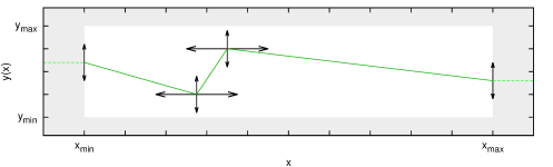
In both applications we seek to model a one-dimensional function using a piecewise linear interpolation scheme between a set of nodes and ask the model selection question “how many nodes are needed to fit the data?”. Thus we place a set of nodes in the plane, where the amplitude and the position are model parameters to be varied. At and fixed-position nodes are placed with varying amplitude only, such that for the model defined by internal nodes there are parameters. As shown in Figure 1, linear interpolation is used to construct at all points (with set constant outside the range ). Of course, other interpolation schemes between nodes may be used, such as splines, although we do not consider these here. The application of these approaches to constraining is described by Vázquez et al. (2012b).
A specific model is defined by how many nodes are used in reconstructing . Comparing multiple models with increasing numbers of nodes identifies how many nodes are needed to fit the data, in other words the preferred complexity inherent in the data. As the final result, one can plot either , where denoted the number of nodes in the most favoured model, or averaged over all models weighted by their posterior odds ratios (PORs) (Parkinson & Liddle, 2013; Planck Collaboration et al., 2015). Either approach identifies clearly the nature of the data constraints on .
The key strength of the reconstruction is its free-form nature, which can capture any shape of function in the plane by adding arbitrarily large numbers of nodes. Providing the model selection criterion penalises over-complex models appropriately by weighing ‘goodness-of-fit’ against the numbers of parameters in the model (Occam’s Razor), identifying how much complexity the data support is performed in a clear and unambiguous manner by the favoured number of nodes. Model selection techniques can thus be used to solve questions on the constraining power of the data, as successfully shown in various cosmological applications (Vázquez et al., 2012a, b; Planck Collaboration et al., 2015).
The nodal reconstructions are clearly nested models. Since our general approach does not require this, for completeness we also consider a non-nested model selection problem by comparing a 2-internal node reconstruction with a sinusoidal model. The rest of this section presents the results obtained and highlights further strengths and weaknesses of our approach.
4.1 Fitting a function to data

Consider a set of data points with experimental errors on each of the points. Assuming there is a functional relationship between the independent variable and dependent variable , captured by , then the likelihood of observing these data is given by:
| (11) |
where are the end points of the uniform region in which the data points may be found a priori. A Bayesian derivation of this likelihood can be found in Appendix A; for more detail see Sivia & Skilling (2006). The integral is calculated numerically using standard quadrature techniques.
Given the data, the Bayesian approach is to use this likelihood to infer the probability distribution of the parameters in some parametric form of the function . We will do this for the family of functions described above, and use posterior odds ratios to determine how many nodes optimally reconstruct the function.
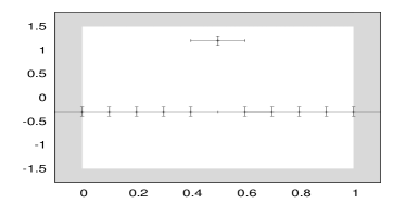
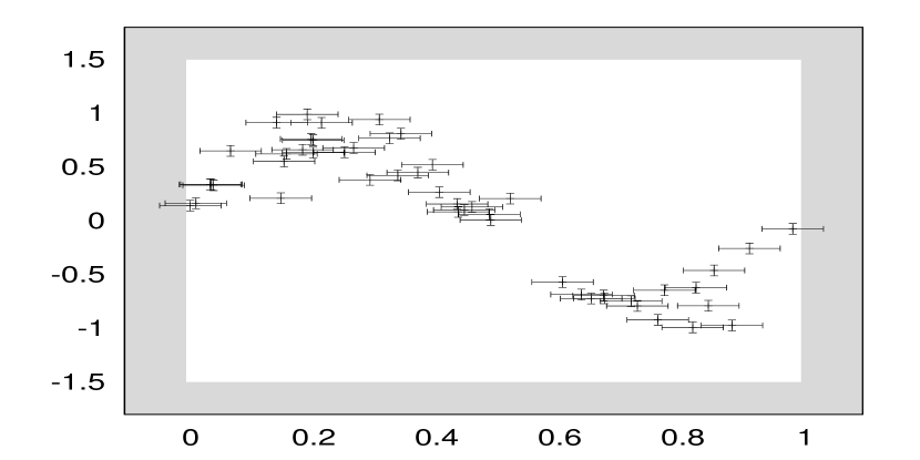
We test 2 different datasets, shown in Figure 2. The traditional evidence-based approach and our new method for calculating posterior odds ratios are compared for each dataset. The constraints on given the data are also discussed.
Dataset (a) has 47 datapoints drawn uniformly in from the function in the range , with each point adjusted in and by random Gaussian noise with mean and (error bars on datapoints are )22250 points were drawn initially for each dataset, but some fellow outside the prior range due to the Gaussian noise, and were not included.. Dataset (b) has 49 datapoints drawn as in (a) but from a piecewise-linear function coinciding with the function at , so that it is very difficult by eye to distinguish the two datasets as being drawn from different functions. We call the function used in (b) for brevity. Clearly, a linearly interpolated nodal model with internal nodes can represent this function exactly.
For each of the datasets we test models with 1 internal node up to 7 internal nodes (i.e. 3 total nodes up to 9 total nodes or 2 line segments up to 8 line segments), using PolyChord (Handley et al., 2015) to calculate evidences (the vanilla method henceforth) and again using PolyChord to implement the new method ( method henceforth)333Note the marginalised posterior probability on is calculated from the chain_unnormalised.txt file using the standard nested sampling technique (Skilling, 2006). It is important to use this file over the usual chain.txt file and set up PolyChord to output all inter-chain points of the algorithm. This ensures good reconstruction of over the lower probability regions in light of the computing ‘log-sum-exp’ problem.. PolyChord is a relatively new nested sampler and was found to be very suitable for this problem. We use uniform priors on the amplitudes of nodes, and sorted uniform priors on the position parameters of nodes, where the priors are uniform but forced to adhere to to avoid the scenario where the internal nodes are interchangeable with each other. We assign equal prior probabilities for each model, so PORs are equal to Bayes factors.
Each dataset is analysed 10 times for each method to determine the statistical uncertainty on the derived PORs. In each case the PORs are normalised to the model with the highest evidence in the vanilla method. Errors on the posterior odds ratios are given as the sample standard deviation from the 10 repeats. PolyChord was run with live points initially to obtain the results labelled , where is the number of parameters to be explored (the dimension of the space) and the number of live points, , is the only tuning parameter associated with the PolyChord sampling algorithm. To highlight accuracy and timing considerations when using the method, we also repeat the analysis with to obtain the results labelled .
4.2 Results for nested nodal models
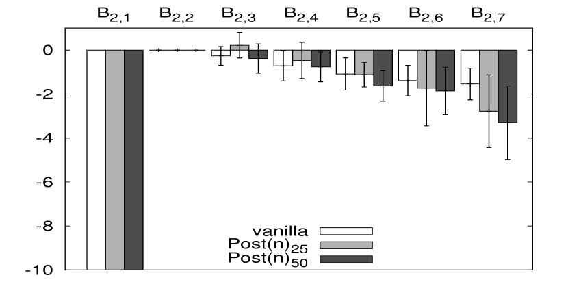
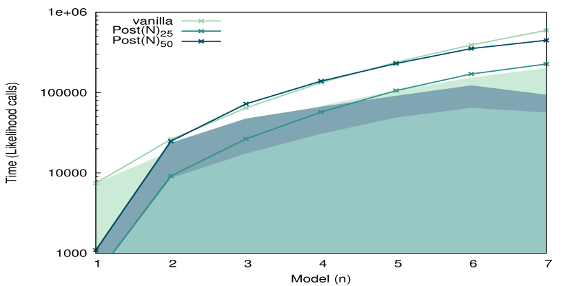
The posterior odds ratios (or Bayes factors) for the vanilla method with and method with and , per dataset, are shown in Figure 3 and show good agreement between the two methods regardless of . From this we conclude that the methods produce consistent posterior odds ratios. As one might expect, for the dataset, the preferred model has internal nodes, whereas a larger number of nodes is preferred for the dataset. The reconstructions of the favoured models for each method are shown in Figures 5 and 6 respectively. The reconstructions are identical in all key features between methods. The graph is not plotted as it was very similar. Finally, the timing data in Figure 4 suggests that results were faster to obtain by about a factor of 2.5 when using the same per parameter, however this comes at a cost in accuracy as the errors on the vanilla posterior odds ratios are clearly tighter than the results. , however, takes less time to produce similar accuracy for the significant posterior odds ratios. In general we observe that our method can produce Bayes factors faster than the vanilla method in a systematic manner, and discuss this in appendix B.
The important discrepancies between the vanilla and methods are in the errors on the posterior odds ratios, where we have identified 2 issues: firstly for large negative posterior odds ratios the errors from the method are quite large and, secondly, the errors on the vanilla method are tighter for equivalent . The first discrepancy might be expected given that PolyChord, and nested samplers in general, rapidly converge to the central peak(s) in a distribution, thus spending less time in lower likelihood regions and sampling those regions proportionately less thoroughly. Given that each model investigated is a separate mode in the computation, a model with low likelihood will be less thoroughly explored than the models with larger likelihoods – making the calculation of less reliable for these models. This is, however, desirable behaviour. Spending compute time only on probable models reduces the overall time taken to find the most probable model(s), whilst the less probable models are still sampled sufficiently well to identify them as less probable.
The second discrepancy is more significant but equally predictable. The number of live points in PolyChord defines how fully the space is explored. For the vanilla method, the calculation provides adequate sampling per model, whilst for the method a similar number of live points needs to explore several models simultaneously, effectively reducing the live points available to explore each model and producing larger errors. This suggests that users need to ensure that algorithm tuning parameters such as are chosen appropriately and check that the results on repetitions of the algorithm are consistent. The results demonstrate clearly that results are confidently extracted in comparable compute-times when best practice is adhered to. Being aware of the increased modality of the space that is inherent to the method and ensuring that the sampling algorithm adequately handles such complex parameter spaces helps ensure accurate results.
Finally, it is worth making some brief comments on the ‘physical’ results of the model selection process for each of the datasets. In dataset (a) a more complex underlying shape in is identified needing more nodes than dataset (b), consistent with the distinction between and . It should be noted too that over-fitting (adding more parameters than needed) is not heavily penalised for dataset (b), as observed in the slow decrease in Bayes factors after the favoured model is found – this is standard behaviour (Sivia & Skilling, 2006, p. 93) and can be understood by considering the Occam factor associated with a parameter which is constrained without increasing the fit of the model (MacKay, 2003, p. 349). In general the model selection and nodal reconstruction technique produces strong conclusions on the shapes of the plane, given the data in each case, and clearly identifies the inherent complexity of the various datasets, as we desired it to.
4.3 Results for non-nested models
Our new method does not require that the models be nested. A model is nested inside another ‘larger’ model if setting some parameters to specific values in the larger model allows one to obtain the smaller nested model. The nodal reconstructions are clearly nested in this sense. Here we quickly demonstrate that our method also works for non-nested models.
We test datasets (a) and (b) against two models. The first model is the sinusoid function and the second model is the 2 internal node reconstruction, so that we expect dataset (a) to favour the sinusoidal model and (b) to favour the linear model. Parameters and are scale parameters for the amplitude and frequency respectively; we assign to these logarithmic priors in the range . Parameters and are shift parameters and we assign uniform priors in the ranges and respectively. These priors reflect sufficient coverage of the prior space defined in Figure 2 and are adequate for comparing the vanilla and new methods. It is important to note that in this test, both the vanilla method and method used . For the vanilla method this resulted in for the sinusoidal model and for the 4 node model, whilst for the method the parameters were searched simultaneously (along with ) to give 11 parameters and .
The posterior odds ratios for dataset (a) favour the sinusoid by and units, for vanilla and methods respectively. The posterior odds ratios for dataset (b) favour the linear model by and units, respectively for vanilla and methods. Taking into account the previous discussion, it is clear that the new method produces posterior odds ratios consistent with the vanilla method. The method here was about per cent slower for dataset (a) and per cent slower for dataset (b). However, with the significantly larger number of live points that the method used, the fact that the methods are of comparable time is a desirable result and suggests that the unconstrained parameters for a given are not significantly increasing the compute time of those isolated nodes in the parameter space.
In general we conclude that the discussions in section 3 regarding unconstrained parameters is correct. When parameters were reviewed for the chains files produced in a given model, the parameters that were not used by that model were distributed according to their priors. This is one of the core strengths and novelties of the method and allows posterior odds ratios to be calculated without constraints on the models to be compared. This verifies that the method works for non-nested models, and we proceed now to apply it to a cosmological application using the nodal reconstruction.
5 Applications to the Dark Energy Equation of State
Having validated our approach on a toy problem, we now apply our method to a cosmological application, for which the vanilla method is not computationally suited. The aim is to demonstrate the method in a typical model selection application to obtain posterior odds ratios efficiently and with estimates of the error that do not require excessive repetition of long computations. We probe the dark energy (DE) equation of state parameter as a function of redshift to update the work of Vázquez et al. (2012b), using more modern datasets. We further showcase the usefulness of the nodal reconstruction approach, briefly described in section 4 and more fully in Vázquez et al. (2012b), in defining the complexity supported by the data and identifying features in , adding to the list of papers using the reconstruction (Vázquez et al., 2012a, b; Aslanyan et al., 2014; Planck Collaboration et al., 2015).
5.1 Method
We combine CMB data from the Planck 2013 data release (Planck Collaboration et al., 2014a, b, c) with the WMAP 9-year polarisation data (Bennett et al., 2013), Baryonic Acoustic Oscillation (BAO) from the BOSS data release 11 (Anderson et al., 2014) and supernovae type Ia (SNIa) data from the Union 2.1 catalogue (Suzuki et al., 2012) to provide constraints on DE behaviour. We focus on the redshift range in the reconstruction, where we set to constant values when . We use the CosmoMC code package (Lewis & Bridle, 2002), which contains the camb code (Lewis et al., 2000; Howlett et al., 2012), and substitute the MCMC sampler for the MultiNest nested sampling plugin running in constant efficiency mode (Feroz & Hobson, 2008; Feroz et al., 2009; Feroz et al., 2013), which is a well established nested sampling implementation for evidence calculations and parameter estimation, and was the sampler used by Vázquez et al. (2012a, b) thereby enabling a direct comparison. To facilitate deviations away from the standard CDM equation of state parameter we implement the ‘Parameterized Post-Friedmann’ framework (PPF) modification to camb (Fang et al., 2008). For further details on the method and datasets see Vázquez et al. (2012b) and Planck Collaboration et al. (2014b) respectively.
Using posterior odds ratios to identify the optimal number of nodes tells us the complexity of features supported by the data. Further, the nodal reconstruction, as shown in the toy model, is highly adept at identifying constraints in the -plane. Of particular interest is whether deviations in away from the successful CDM cosmological model are supported by modern data and to identify which DE extensions are favoured. Theories incorporating deviations from include quintessence scalar fields for (Ratra & Peebles, 1988; Caldwell et al., 1998; Tsujikawa, 2013) and phantom DE models with super-negative (Caldwell, 2002; Sahni, 2005). The possibility of crossing of the phantom divide line at in dynamical models has also been considered (Zhang, 2009). Modified gravity or brane-world models also make predictions about (Sahni, 2005). Thus, paramount to understanding DE is determining .
To do this we compare 6 models, in order of increasing complexity: CDM with , CDM with constant in but allowed to vary in amplitude, CDM with and allowed to vary and linear interpolation for between them (0 internal node model), and then nodal models with , and internal nodes respectively. Models are abbreviated to , , , , and respectively, where appropriate. Priors on each parameter are uniform on the range and were chosen to be conservative, we did not check the robustness of results with respect to prior choice and leave this for future work, see Vázquez et al. (2012b) for such an analysis. Priors on each parameter are uniform on such that for more than one internal node (i.e. sorted uniform priors as in the toy model). The previous work by Vázquez et al. (2012b) found that CDM was favoured, whilst the internal node model had the second largest evidence, pointing to structure in that could not be captured by a constant equation of state parameter CDM, or even the internal node model. Here we show clearly that Planck 2013 era datasets do not have this feature and only CDM can be considered favoured.
| Parameter | Prior Range | Prior Type |
|---|---|---|
| Uniform | ||
| Uniform | ||
| Uniform | ||
| Uniform | ||
| Uniform | ||
| Uniform | ||
| Uniform | ||
| Uniform | ||
| Uniform | ||
| Uniform | ||
| Uniform | ||
| Uniform | ||
| Uniform | ||
| Uniform | ||
| Uniform | ||
| Uniform | ||
| Uniform | ||
| Uniform | ||
| Uniform | ||
| Uniform | ||
| Uniform | ||
| Sorted-uniform | ||
| Uniform | ||
| Uniform |
An important point is that the Planck data require the addition of 14 so called nuisance parameters. These must be sampled and, together with the 6 parameters of CDM models, produce an at least 20 dimensional parameter space. As MultiNest is a rejection nested sampling algorithm, it is expected that computation times increase significantly in higher dimensions as the volume on the shell increases444Specifically, it constructs multi-dimensional ellipsoids to estimate sampling within an iso-likelihood region, as required by nested sampling. The ellipsoids expand by a fraction to ensure no viable regions of the true iso-likelihood contour are outside this estimate. Points are sampled inside these ellipsoids and rejected until meeting the nested sampling criterion.. MultiNest has the algorithm search parameters and , where decreasing (in constant efficiency mode) typically achieves more accurate results more effectively than increasing .
With the new method there seems to be no way to estimate the errors on the posterior odds ratios from a single run, and attaining these is best done via repeat simulation and the calculation of sample standard deviations from these. We therefore performed 3 repetitions each using with (the repeat runs) and the default July 2014 CosmoMC priors for the 20 CDM and nuisance parameters and the priors mentioned above for additional model parameters; an overview is shown in Table 2. Constant efficiency mode had to be used to attain feasible computing times, similarly the search parameters could not just be increased arbitrarily. With these MultiNest search parameters and constant efficiency mode, it was found that the edges of the priors were not sampled effectively. The error is reproducible with a 20-dimensional Gaussian test likelihood with a covariance matrix given by Planck chains. To ensure this problem had no impact on our results, firstly we added a prior for an unconstrained parameter, the parameter in Table 2, which should produce a flat posterior. Observing the edge effects problem on this parameter gives a clear indication of the severity of the problem, and allows us to reconsider parameter estimation conclusions if needed. Secondly we tested for convergence of the marginalised posterior on with respect to search parameter changes to ensure that our parameter estimation results were robust. We thus performed a single further run using MultiNest with the search parameters , (full run) for which the edges of the prior were sampled effectively. Given the concerns about the accuracy of the MultiNest evidence calculation for Planck data (due to nuisance parameters, high dimensionality, and the need for constant efficiency mode), the new method combined with the 2 robustness checks thus provides a valuable alternative way to obtain posterior odds ratios.
5.2 Results
| Bayes Factor | Full Run | Repeat Averages |
|---|---|---|
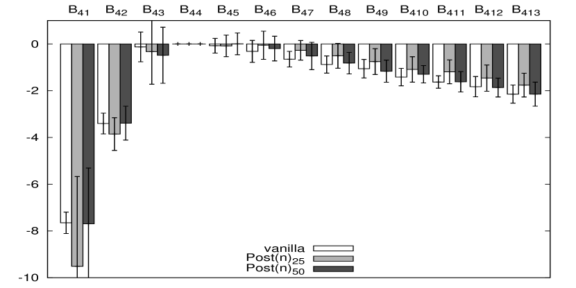
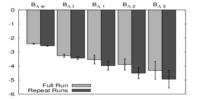
The posterior odds ratio results for the full run and the 3 repeat runs are shown in Figure 7 and Table 3. The key points are firstly that the posterior odds ratios are consistent with each other, demonstrating convergence of with respect to MultiNest search parameters, and secondly that the investigation clearly favours CDM.
The toy model showed that error bars on posterior odds ratios will depend on how thoroughly the sampling explores the space. Note that the error bars used are the sample standard deviations from the posterior odds ratios of the 3 repeat runs. The repeat run posterior odds ratios are consistent with the full run and sufficiently tight to resolve differences to make conclusions based on Jeffreys guideline, suggesting that the space is well explored. This convergence on reruns, together with the convergence between different MultiNest search parameters, suggests that the posterior odds ratio results are robust. Additionally, the edge effect problem previously mentioned was thoroughly checked for using an unconstrained parameter . The posterior of was close to flat for all runs. The edge effect problem presumably affects all parameters a small amount, as the strength of this effect is different between the different MultiNest search parameter settings whilst the posterior odds ratios are consistent, it suggests that the posterior odds ratios are not significantly biased. From these 4 runs we therefore conclude that we have accurate posterior odds ratios and proceed to quote those of the full run combined with the errors from the 3 repeat runs as upper estimates for those of the full run (as repeats of a more well sampled run will produce tighter estimates, shown in the toy model when doubling ).
From these posterior odds ratios it is clear that CDM is the only favourable model. The decrease in posterior odds ratios with an increase in the number of parameters to model DE suggests that further additions of parameters to model deviations from CDM are penalised more strongly by the Occam’s Razor principle than the gain in constraining power that they provide. One can estimate the Occam factor associated with adding an additional nodal amplitude parameter, using the analysis in (MacKay, 2003, page 349), as , where is the width around the peak of a Laplace approximation inside the evidence integral and is the prior width. We estimating for non-Gaussian parameters with a full width half max (FWHM) calculation of the 1D marginalised -amplitude posterior. Doing this for the CDM model’s additional parameter yields a drop in the Bayes factor due to the approximated Occam factor of . The observed therefor suggests that the parameter is not improving the likelihood fit to the data significantly. Doing something similar for the internal node model gives an Occam factor of (using the average of the 5 amplitudes; assuming that an additional -position parameter is unconstrained as there are no additional features it would constrain). This is the anticipated decay in the posterior odds ratio when adding unnecessary nodes, and the Bayes factor drop from CDM to CDM at suggests that nodes already saturate the space.
A clear and strong conclusion from this analysis is that there is considerably less evidence for deviations from CDM in the Planck era datasets used here than in the WMAP era datasets used by Vázquez et al. (2012b), which is consistent with other results (Planck Collaboration et al., 2014b; Shafer & Huterer, 2014). The next most favoured model is the next simplest one, CDM, and at a posterior odds ratios of it is almost significantly disfavoured according to the Jeffreys guideline. All other models are significantly disfavoured at between to log units.
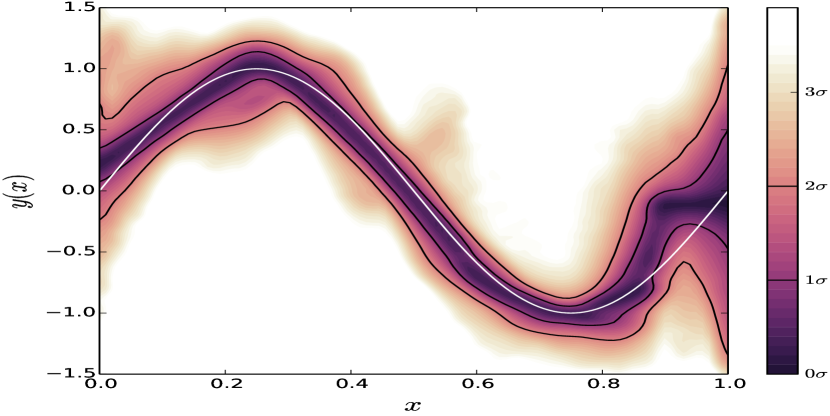
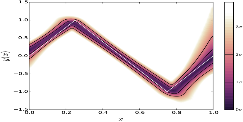
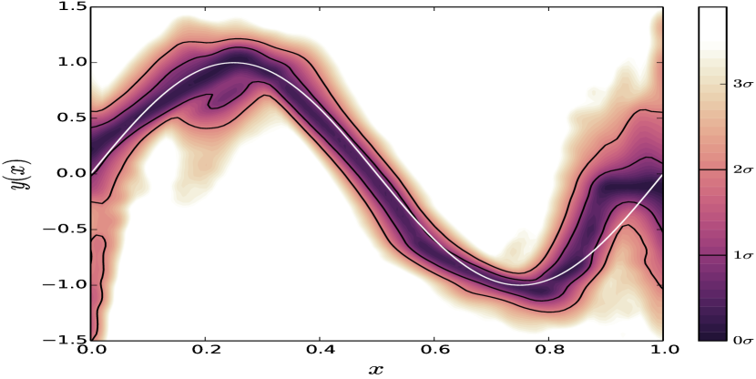
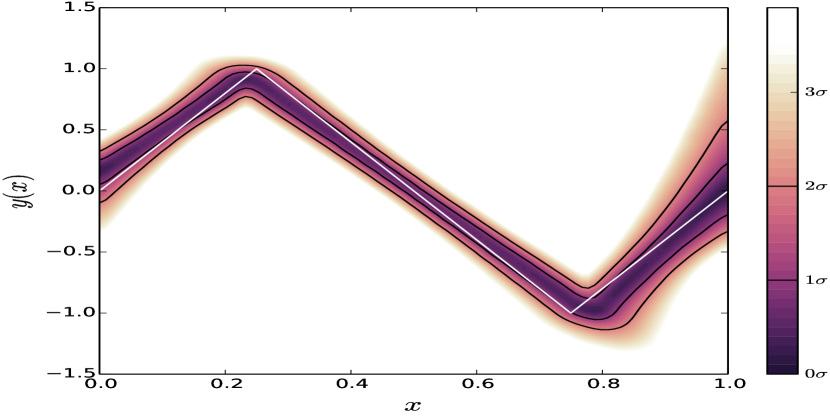
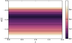
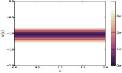
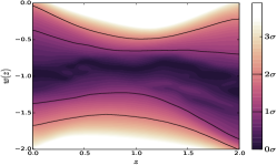
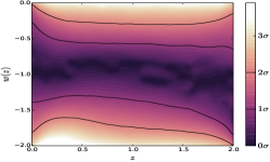
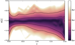
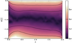
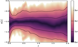
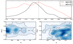
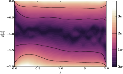
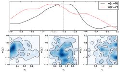
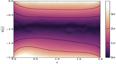
The constraints in the -plane for each of the model extensions beyond CDM, shown in Figure 8, do however indicate some deviations from . Typically the data seem to favour the phantom region, potentially more so at the ends of the considered redshift range and less so at redshift , where the data gives the tightest constraints. However, the and contours clearly indicate that these effects are not significant. At all and for all models, is comfortably within the peak of the distribution and more so in the regions where we have strong data constraints, suggesting that any deviations or apparent systematic patterns are dominated by a lack of data. The plane reconstructions also support the model selection conclusions that CDM is significantly favoured over other models, as the constraints in the data do not deviate from beyond even .
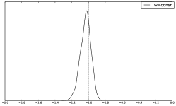
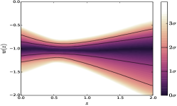
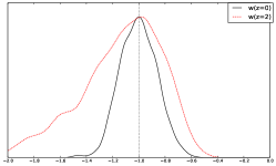
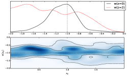
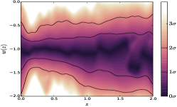
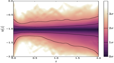
The correct Bayesian way to view the plane reconstructions for all models considered is to sum over all the models whilst weighting by the Bayesian evidence, or equivalently posterior odds ratios. This is exceptionally easy to implement with our new method, as a program like GetDist (included with CosmoMC) can use the chains file produced by the new method to correctly weight all the models automatically whilst marginalising out the parameter . Figure 9 shows this for the 5 DE extension models beyond CDM. When plotting with CDM the plot is centered on , with 85 per cent of the peak confidence interval region contained in the line, and thus a plot showing only the model extensions is more insightful. The plane reconstruction shows clearly the constraining power of the data at different redshifts as our knowledge of moves from the prior on the left to the posterior on the right. The result is a tightly constrained function of slightly below for all redshifts, suggesting a small favouring of the phantom region at an insignificant level. Most importantly, CDM is fully compatible, well within of the model extension results, as is expected given the Bayesian model selection analysis. This insignificant deviation away from explains clearly why CDM is so heavily favoured.
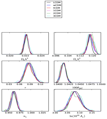
Of practical importance is the strength with which the nodal reconstruction identifies features, and especially that the reconstruction is data driven. Most of our datasets that can constrain are in the redshift range and this is shown by where the reconstructions most tightly constrain the plane. This reconstruction technique is clearly of merit and in the future, with more powerful datasets, can hopefully act as a tool to identify features (if any) in . At present, the work here can only suggest that dark energy models with close to are needed. Finally, the posteriors of the CDM parameters are plotted in Figure 10 for each of the 6 models tested. The posteriors of the DE extensions agree well with the CDM values, as can be expected given that there is no significant deviation from .
6 Conclusions
We demonstrated a novel method for calculating posterior odds ratios through a toy model application and then applied it to a cosmological model selection problem.
Our new method uses Bayesian parameter estimation on a parameter that switches between models, via a hyper-likelihood that wraps around the individual model likelihoods, to infer posterior odds ratios (or Bayes factors if desired) without calculating evidences. It uses novel partitioning of the parameter space via the parameter , and marginalisation of posterior probabilities, to allow sampling of a variable length parameter space when moving between models, thus facilitating any models to be tested without restriction and without reversible jump Monte Carlo techniques. To use the method one needs to have a parameter estimation algorithm capable of sampling from multi-modal spaces and to decide which models one wants to test a priori.
The toy model demonstrated clearly that the method is valid and consistent with the existing method of calculating posterior odds ratios by evaluating evidences. We conclude that the new method is not necessarily faster, despite avoiding evidence integrals, for 2 reasons. Firstly, to get errors on the posterior odds ratios it requires rerunning several times, whereas nested sampling algorithms such as MultiNest and PolyChord can attain error estimates of evidences from a single run. Secondly, the parameter space needs to be explored comparably thoroughly in both methods, as shown by the increase in error bars on the posterior odds ratios in the toy model when spending less computational time on the new method.
A peculiar feature of the new method in combination with nested sampling (which likely applies to other samplers too) is that computation time dedicated to a model is dependent on how strongly the model is favoured over others. Less favoured models become depopulated with live points as the nested sampling algorithm removes lowest likelihood points. As a result, we observed that less favoured models typically had less accurate posterior odds ratio calculations, which helps to reduce computing time, but still in such a way that they were always identifiable as less favoured. The reduction in computing time can be substantial, especially in applications where there are a number of computationally expensive models with low posterior odds ratios.
The toy models illuminated precautionary measures that best be adhered to by users. As with all Bayesian parameter estimation, robustness of posterior probabilities to changes in algorithm-specific tuning parameters needs to be tested for and in the case of the new method, where a posterior is used to infer evidence ratios, it is especially important to check this. It is best to test that the posterior odds ratios obtained from the posterior on are consistent on repetitions of the algorithm and also that the error bars attained from repetitions are sufficiently small if needing to make judgments based on Jeffreys guideline. The toy model also highlighted the strength of the nodal reconstruction in identifying features in plane reconstruction problems. We conclude that it is a useful tool for analysing the complexity supported by the data and add to the volume of literature using it (Vázquez et al., 2012a, b; Aslanyan et al., 2014; Planck Collaboration et al., 2015).
Thereafter, taking the above considerations into account, the new method was used to attain posterior odds ratios in a cosmological context where direct evaluation of evidences can be computationally demanding and problematic. We applied the nodal reconstruction technique to reconstruct the dark energy redshift-dependent equation of state parameter , analysing the dynamic behaviour supported by modern datasets in a search for deviations from the CDM model (). This was principally an update on a paper using WMAP era data by Vázquez et al. (2012b). We concluded that CDM is significantly favoured above any nodal reconstruction applied. Additionally, the model allowing to vary as a constant is almost significantly disfavoured at log-units of the posterior odds ratio with respect to CDM. We conclude that additional parameters are systematically disfavoured: increasing the complexity of the reconstruction decreases posterior odds ratios with respect to CDM. The Occam’s Razor effect penalises additional parameters when using posterior odds ratios to do model selection and, as CDM is an excellent fit to current cosmological data, the addition of parameters to extended beyond CDM adds less to the constraining power of the models than the Occam’s factor penalises.
The robustness of the results and methods were confirmed in several ways. Figure 10 shows that the CDM parameters of each of the dark energy extension models agree well with the CDM values, as is expected given that all models agree well with . Further, a potential problem in sampling the edges of priors in high-dimensions was identified with MultiNest when using constant efficiency mode, but through tracking an unconstrained parameter , it was shown to be insignificant given the final search parameters used. General robustness of the new method was confirmed too by repeating the calculation of with different search parameters and showing that the value of had converged with respect to algorithm tuning parameter.
Finally, the cosmological application demonstrated the strength of the new method, attaining posterior odds ratios without needing evidence calculations and effectively dealing with parameter spaces of varying length. Errors on the posterior odds ratios were attained through repeat runs with a faster sampling parameter setup which doubled to confirm that the posterior odds ratios were converged and accurate. As such a robustness check is important for any parameter estimation or model selection problem, where an algorithm uses tuning parameters for the sampling, this approach should come at little extra cost in practice.
Acknowledgments
The authors thank Farhan Feroz for many useful discussions and insights, and also Ewan Cameron, Kirill Tchernyshyov and the journal referee for their very insightful additions. This work was performed using the Darwin Supercomputer of the University of Cambridge High Performance Computing Service (http://www.hpc.cam.ac.uk/), provided by Dell Inc. using Strategic Research Infrastructure Funding from the Higher Education Funding Council for England and funding from the Science and Technology Facilities Council. Parts of this work were undertaken on the COSMOS Shared Memory system at DAMTP, University of Cambridge operated on behalf of the STFC DiRAC HPC Facility, this equipment is funded by BIS National E-infrastructure capital grant ST/J005673/1 and STFC grants ST/H008586/1, ST/K00333X/1. SH and WH thank STFC for financial support.
References
- Akaike (1974) Akaike H., 1974, IEEE Trans. Auto. Control, 19, 716
- Anderson et al. (2014) Anderson L., et al., 2014, MNRAS, 441, 24
- Aslanyan et al. (2014) Aslanyan G., Price L. C., Abazajian K. N., Easther R., 2014, J. Cosmology Astropart. Phys., 8, 52
- Bayes & Price (1763) Bayes M., Price M., 1763, An Essay towards Solving a Problem in the Doctrine of Chances. By the Late Rev. Mr. Bayes, F. R. S. Communicated by Mr. Price, in a Letter to John Canton, A. M. F. R. S.
- Bennett et al. (2013) Bennett C. L., et al., 2013, ApJS, 208, 20
- Brewer & Donovan (2015) Brewer B. J., Donovan C. P., 2015, MNRAS, 448, 3206
- Brewer et al. (2011) Brewer B. J., Pártay L. B., Csányi G., 2011, Stat. Comput., 21, 649
- Caldwell (2002) Caldwell R., 2002, Phys. Lett. B, 545, 23
- Caldwell et al. (1998) Caldwell R., Dave R., Steinhardt P., 1998, Phys. Rev. Lett., 80, 1582
- Carlin & Chib (1995) Carlin B. P., Chib S., 1995, J. Royal Stat. Soc. Series B (Methodological), 57, 473
- Clyde et al. (2007) Clyde M. A., Berger J. O., Bullard F., Ford E. B., Jefferys W. H., Luo R., Paulo R., Loredo T., 2007, in Babu G. J., Feigelson E. D., eds, Astronomical Society of the Pacific Conference Series Vol. 371, Statical Challenges in Modern Astronomy IV. p. 224
- Fang et al. (2008) Fang W., Hu W., Lewis A., 2008, Phys. Rev. D, 78, 087303
- Feroz & Hobson (2008) Feroz F., Hobson M. P., 2008, MNRAS, 384, 449
- Feroz & Skilling (2013) Feroz F., Skilling J., 2013, in AIP Conf. Proc.. pp 106–113
- Feroz et al. (2009) Feroz F., Hobson M. P., Bridges M., 2009, MNRAS, 398, 1601
- Feroz et al. (2013) Feroz F., Hobson M. P., Cameron E., Pettitt A. N., 2013, preprint (arXiv:1306.2144)
- Gelman & Meng (1998) Gelman A., Meng X.-L., 1998, Stat. Sci., 13, 163
- Goyder & Lasenby (2004) Goyder R., Lasenby A. N., 2004, MNRAS, 353, 338
- Green (1995) Green P. J., 1995, Biometrica, 82, 711
- Green (2011) Green D. A., 2011, Bull. Astron. Soc. India, 39, 289
- Handley et al. (2015) Handley W. J., Hobson M. P., Lasenby A. N., 2015, MNRAS, 450, L61
- Hobson & McLachlan (2003) Hobson M. P., McLachlan C., 2003, MNRAS, 338, 765
- Howlett et al. (2012) Howlett C., Lewis A., Hall A., Challinor A., 2012, J. Cosmology Astropart. Phys., 2012, 27
- Jeffreys (1961) Jeffreys S. H., 1961, The Theory of Probability. Oxford University Press
- Lewis & Bridle (2002) Lewis A., Bridle S., 2002, Phys. Rev. D, 66, 103511
- Lewis et al. (2000) Lewis A., Challinor A., Lasenby A., 2000, ApJ, 538, 473
- Liddle et al. (2006) Liddle A., Mukherjee P., Parkinson D., 2006, Astron. & Geophys., 47, 4.30
- Lodewyckx et al. (2011) Lodewyckx T., Kim W., Lee M. D., Tuerlinckx F., Kuppens P., Wagenmakers E.-J., 2011, J. Mathematical Psychology, 55, 331
- MacKay (2003) MacKay D. J. C., 2003, Information Theory, Inference and Learning Algorithms. Cambridge University Press
- Parkinson & Liddle (2013) Parkinson D., Liddle A. R., 2013, Stat. Analysis & Data Mining, 6, 3
- Planck Collaboration et al. (2014a) Planck Collaboration et al., 2014a, A&A, 571, A15
- Planck Collaboration et al. (2014b) Planck Collaboration et al., 2014b, A&A, 571, A16
- Planck Collaboration et al. (2014c) Planck Collaboration et al., 2014c, A&A, 571, A17
- Planck Collaboration et al. (2015) Planck Collaboration et al., 2015, preprint (arXiv:1502.02114)
- Ratra & Peebles (1988) Ratra B., Peebles P., 1988, Phys. Rev. D, 37, 3406
- Sahni (2005) Sahni V., 2005, in Tamvakis K., ed., Lect. Notes Phys., Berlin Springer Verlag Vol. 653, The Physics of the Early Universe. p. 141
- Schwarz (1978) Schwarz G., 1978, Ann. Stat., 6, 461
- Shafer & Huterer (2014) Shafer D. L., Huterer D., 2014, Phys. Rev. D, 89, 063510
- Sisson (2005) Sisson S. A., 2005, J. American Stat. Assoc., 100, 1077
- Sivia & Skilling (2006) Sivia D. S., Skilling J., 2006, Data analysis: a Bayesian tutorial. Oxford University Press
- Skilling (2004) Skilling J., 2004, American Inst. Phys. Conf. Series, 119, 1211
- Skilling (2006) Skilling J., 2006, Bayesian Analysis, 1, 833
- Suzuki et al. (2012) Suzuki N., Rubin D., Lidman C., Aldering G., Amanullah R., Others 2012, ApJ, 746, 85
- Tierney & B. (1986) Tierney L., B. K. J., 1986, J. American Stat. Assoc., 81, 82
- Trotta (2008) Trotta R., 2008, Contemporary Phys., 49, 71
- Tsujikawa (2013) Tsujikawa S., 2013, Class. Quant. Grav., 30, 214003
- Vázquez et al. (2012a) Vázquez J. A., Bridges M., Hobson M., Lasenby A., 2012a, J. Cosmology Astropart. Phys., 2012, 6
- Vázquez et al. (2012b) Vázquez J. A., Bridges M., Hobson M., Lasenby A., 2012b, J. Cosmology Astropart. Phys., 2012, 20
- Verdinelli & Wasserman (1995) Verdinelli I., Wasserman L., 1995, J. American Stat. Assoc., 90, 614
- Zhang (2009) Zhang H., 2009, preprint (arXiv:0909.3013)
Appendix A Line fitting Likelihood
We aim to fit a parametric function to a set of data points , where we have some knowledge of the errors on these measurements (). In order to fit the function, one needs to calculate the likelihood of observing the data , given the function , the observed errors and any additional assumptions we must make :
| (12) |
To model the “error bars”, we assume that each of the data points is drawn from a separable Gaussian distribution with covariance . The distribution will be centered about some true value , where these values are unknown and will need to be marginalised over as nuisance parameters in the final calculation. If each of these distributions are independent from each other, we arrive at the likelihood:
| (13) |
To marginalise out the nuisance parameters, we place our prior assumptions on them. We shall assume that the true values are drawn uniformly in some range , and we shall assume that the true obey the functional relationship: . Given this, the probability distribution is:
| (14) |
where is the Dirac -function. Multiplying (13) and (14) together and marginalising out by integrating yields the likelihood:
| (15) |
This procedure may be straightforwardly extended to consider correlated error bars where the covariance matrix of (13) is no longer diagonal. One may also adjust (14) if some additional knowledge is known about the independent variables . For further details the reader is referred to Sivia & Skilling (2006).
Appendix B Efficient computing of Bayes factors
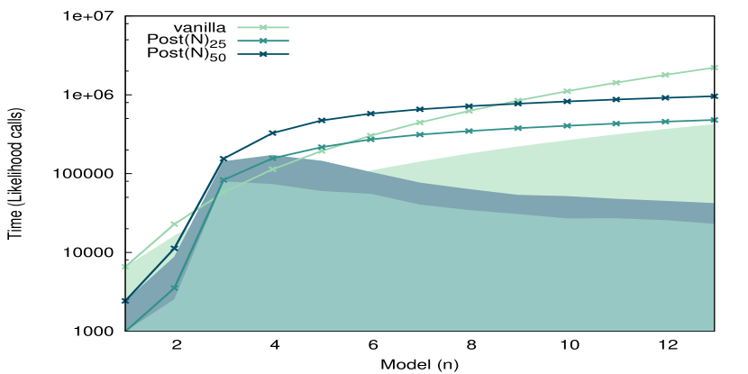
Using the datapoints in figure 11 to test the vanilla and methods we demonstrate that our new method may outperform the evidences approach in a systematic fashion that makes the approach desirable for common astrophysical and cosmological problems.
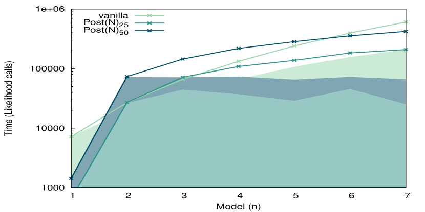
Running the nodal reconstruction technique with models of internal node up to internal nodes ( to total nodes) we obtain Bayes factors and timing results shown in figure 12. The timing data shows the number of posterior points, and thus likelihood calculations up to a factor of the PolyChord efficiency, that each method makes for each of the nodal reconstruction models (shaded plots), alongside the cumulative number of likelihood calculations of these models (line plots).
Using the vanilla method, completing the evidence calculation for each model means that adding increasingly complex models is increasingly computationally expensive. In the method, however, the model space is rapidly traversed from lower likelihood regions to higher likelihood regions, so that computationally expensive models with low likelihoods (or more correctly, with lower Bayes factors compared to other models in the space) are explored rapidly by the nested sampling algorithm. This is clearly identified by the fact that the Bayes factors and the number of likelihood calculations peak at the same model ( internal nodes) and tail off similarly for models on either side of this.
It is worth noting, however, that the method performs more likelihood calculations for the most probable models, because the additional overhead of setting up the other parameters and populating their dimensions with live points (because throughout we use that ) means that the algorithm progresses more slowly.
Astrophysical and cosmological problems where a number of models of increasing complexity are explored may therefor benefit from using this method. It is not guaranteed, however, as with the vanilla case one may have identified a drop off in the Bayes factors beyond and stopped testing the more complex models thereafter. Nonetheless, the method could provide an efficient means of verifying the drop off (for example one might run the above with as a fast means of verifying the shape). Any gains in performance must be considered against the need for repetition of the algorithm to obtain an estimate of the error on the Bayes factors.