Online Learning to Sample
Abstract
Stochastic Gradient Descent (SGD) is one of the most widely used techniques for online optimization in machine learning. In this work, we accelerate SGD by adaptively learning how to sample the most useful training examples at each time step. First, we show that SGD can be used to learn the best possible sampling distribution of an importance sampling estimator. Second, we show that the sampling distribution of an SGD algorithm can be estimated online by incrementally minimizing the variance of the gradient. The resulting algorithm — called Adaptive Weighted SGD (AW-SGD) — maintains a set of parameters to optimize, as well as a set of parameters to sample learning examples. We show that AW-SGD yields faster convergence in three different applications: (i) image classification with deep features, where the sampling of images depends on their labels, (ii) matrix factorization, where rows and columns are not sampled uniformly, and (iii) reinforcement learning, where the optimized and exploration policies are estimated at the same time, where our approach corresponds to an off-policy gradient algorithm.
1 Introduction
In many real-world problems, one has to face intractable integrals, such as averaging on combinatorial spaces or non-Gaussian integrals. Stochastic approximation is a class of methods introduced in 1951 by Herbert Robbins and Sutton Monro [1] to solve intractable equations by using a sequence of approximate and random evaluations. Stochastic Gradient Descent [2] is a special type of stochastic approximation method that is widely used in large scale learning tasks thanks to its good generalization properties [3].
Stochastic Gradient Descent (SGD) can be used to minimize functions of the form:
| (1) |
where is a known fixed distribution and is a function that maps into , i.e. a family of functions on the metric space and parameterized by . SGD is a stochastic approximation method that consists in doing approximate gradient steps equal on average to the true gradient [2]. In many applications, including supervised learning techniques, the function is the log-likelihood and is an empirical distribution with density where is a set of i.i.d. data sampled from an unknown distribution.
At a given step , SGD can be viewed as a two-step procedure: (i) sampling according to the distribution ; (ii) doing an approximate gradient step with step-size :
| (2) |
The convergence properties of SGD are directly linked to the variance of the gradient estimate [4]. Consequently, some improvements on this basic algorithm focus on the use of (i) parameter averaging [5] to reduce the variance of the final estimator, (ii) the sampling of mini-batches [6] when multiple points are sampled at the same time to reduce the variance of the gradient, and (iii) the use of adaptive step sizes to have per-dimension learning rates, e.g., AdaGrad [7].
In this paper, we propose another general technique, which can be used in conjunction with the aforementioned ones, which is to reduce the gradient variance by learning how to sample training points. Rather than learning the fixed optimal sampling distribution and then optimizing the gradient, we propose to dynamically learn an optimal sampling distribution at the same time as the original SGD algorithm. Our formulation uses a stochastic process that focuses on the minimization of the gradient variance, which amounts to do an additional SGD step (to minimize gradient variance) along each SGD step (to minimize the learning objective). There is a constant extra cost to pay at each iteration, but it is the same for each iteration, and when simulations are expensive or the data access is slow, this extra computational cost is compensated by the increase of convergence speed, as quantified in our experiments.
The paper is organized as follows. After reviewing the related work in Section 2, we show that SGD can be used to find the optimal sampling distribution of an importance sampling estimator (Sec. 3). This variance reduction technique is then used during the iterations of a SGD algorithm by learning how to reduce the variance of the gradient (Sec. 4). We then illustrate this algorithm — called Adaptive Weighted SGD (AW-SGD) — on three well known machine learning problems: image classification (Sec. 5), matrix factorization (Sec. 6), and reinforcement learning (Sec. 7). Finally, we conclude with a discussion (Sec. 9).
2 Related work
The idea of speeding up learning by modifying the importance sampling distribution in SGD has been recently analyzed by [8] who showed that a particular choice of the sampling distribution could lead to sub-linear performance guarantees for support vector machines. We can see our approach as a generalization of this idea to other models, by including the learning of the sampling distribution as part of the optimization. The work of [9] shows that using a simple model to choose which data to resample from is a useful thing to do, but they do not learn the sampling model while optimizing. The two approaches mentioned above can be viewed as the extreme case of adaptive sampling, where there is one step to learn the sampling distribution, and then a second step to learn the model using this sampling distribution. The training on language models has been shown to be faster with adaptive importance sampling [10; 11], but the authors did not directly minimize the variance of the estimator.
Regarding variance reduction techniques, in addition to the aforementioned ones (Polyak-Ruppert Averaging [5], batching [6], and adaptive learning rates like AdaGrad [7]), an additional technique is to use control variates (see for instance [12]). It has been recently used by [13] to estimate non-conjugate potentials in a variational stochastic gradient algorithm. The techniques described in this paper can also be straightforwardly extended to the optimization of a control variate. A full derivation is given in the appendix, but it was not implemented in the experimental section. In the neural net community, adapting the order at which the training samples are used is called curriculum learning [14], and our approach can be seen under this framework, allthough our algorithm is more general as it can speadup the learning on arbitrary integrals, not only sums of losses over the training data.
Another way to obtain good convergence properties is to properly scale or rotate the gradient, ideally in the direction of the inverse Hessian, but this type of second-order method is slow in practice. However, one can estimate the Hessian greedily, as done in Quasi-Newton methods such as Limited Memory BFGS, and then adapt it for the SGD algorithm, similarly to [6].
3 Adaptive Importance Sampling
We first show in this section that SGD is a powerful tool to optimize the sampling distribution of Monte Carlo estimators. This will motivate our Adaptive Weighted SGD algorithm in which the sampling distribution is not kept constant, but learned during the optimization process.
We consider a family of sampling distributions on , such that is absolutely continuous with respect to (i.e. the support of is included in the support of ) for any in the parametric set . We denote the density . Importance sampling is a common method to estimate the integral in Eq. (1). It corresponds to a Monte Carlo estimator of the form (we omit the dependency on for clarity):
| (3) |
where is called the importance distribution. It is an unbiased estimator of , i.e. the expectation of is exactly the desired quantity .
To compare estimators, we can use a variance criterion. The variance of this estimator depends on :
| (4) |
where and denote the expectation and variance with respect to distribution .
To find the best possible sampling distribution in the sampling family , one can minimize the variance with respect to . If belongs to the family , then there exists a parameter such that -almost surely. In such a case, the variance of the estimator is null: one can estimate the integral with a single sample. In general, however, the parametric family does not contain a normalized version of . In addition, the minimization of the variance has often no closed form solution. This motivates the use of approximate variance reduction methods.
A possible approach is to minimize with respect to the importance parameter . The gradient is:
| (5) | |||||
This quantity has no closed form solution, but we can use a SGD algorithm with a gradient step equal on average to this quantity. To obtain an estimator of the gradient with expectation given by Equation (3), it is enough to sample a point according to and then set . This is then repeated until convergence. The full iterative procedure is summarized in Algorithm 1.
In the experiments below, we show that learning the importance weight of an importance sampling estimator using SGD can lead to a significant speed-up in several machine learning applications, including the estimation of empirical loss functions and the evaluation of a policy in a reinforcement learning scenario. In the following, we show that this idea can also be used in a sequential setting (the function can change over time), and when has multivariate outputs, so that we can control the variance of the gradient of a standard SGD algorithm and, ultimately, speedup the convergence.
4 Biased Sampling in Stochastic Optimization
In this section, we first analyze a weighted version of the SGD algorithm where points are sampled non-uniformly, similarly to importance sampling, and then derive an adaptive version of this algorithm, where the sampling distribution evolves with the iterations.
4.1 Weighted stochastic gradient descent
As introduced previously, our goal is to minimize the expectation of a parametric function (cf. Eq. (1)). Similarly to importance sampling, we do not need to sample according to the base distribution at each iteration of SGD. Instead, we can use any distribution defined on if each gradient step is properly re-weighted by the density . Each iteration of the algorithm consists in two steps: (i) sample according to distribution ; (ii) do an approximate gradient step:
| (7) |
Depending on the importance distribution , this algorithm can have different convergence properties from the original SGD algorithm. As mentioned previously, the best sampling distribution would be the one that gives a small variance to the weighted gradient in Eq. (7). The main issue is that it depends on the parameters , which are different at each iteration.
Our main observation is that we can minimize the variance of the gradient using the previous iterates, under the assumption that this variance does not change to quickly when is updated. We argue this is reasonable in practice as learning rate policies for usually assume a small constant learning rate, or a decreasing schedule [2]. In the next section, we build on that observation to build a new algorithm that learns the best sampling distribution in an online fashion.
4.2 Adaptive weighted stochastic gradient descent
Similarly to Section 3, we consider a family of sampling distributions parameterized by in the parametric set . Using the sampling distribution with p.d.f. , we can now evaluate the efficiency of the sampling distributions based on the variance :
| (8) | ||||
| (9) |
For a given function we would like to find the parameter of the sampling distribution that minimizes the trace of the covariance , i.e.:
| (10) |
Note that if the family of sampling distribution belongs to the exponential family, the problem (10) is convex, and therefore can be solved using (sub-) gradient methods. Consequently, a simple SGD algorithm with gradient steps having small variance consists in the following two steps at each iteration :
-
1.
perform a weighted stochastic gradient step using distribution to obtain ;
-
2.
compute by solving Equation (10), i.e. find the parameter minimizing the variance of the gradient at point . This can be done approximately by applying steps of stochastic gradient descent.
The inner-loop SGD algorithm involved in the second step can be based on the current sample, and the stochastic gradient direction is
| (11) | ||||
In practice, we noted that it is enough to do a single step of the inner loop, i.e. . We call this simplified algorithm the Adapted-Weighted SGD Algorithm and its pseudocode is given in Algorithm 2. We see that AW-SGD is a slight modification of the standard SGD — or any variant of it, such as Adagrad, AdaDelta or RMSProp – but where the sampling distribution evolves during the algorithm, thanks to the update of . This algorithm is useful when the gradient has a variance that can be significantly reduced by choosing better samples. An important design choice of the algorithm is the choice of the decay of the step sizes sequences and . While using adaptive step sizes appears to be useful in some settings, it appears that the regime in which AW-SGD outperforms SGD is when are significantly larger than , meaning that the algorithm converges quickly to the smallest variance, and AW-SGD tracks it during the course of the iterations. Ideally, the sequence of sampling parameters remains close to the optimal trajectory which consist is the best possible sequence of sampling parameters given by Equation 10
We now illustrate the benefit of this algorithm in three different applications: image classification, matrix factorization and reinforcement learning.
5 Application to Image classification
Large scale image classification is an important machine learning tasks where images containing a given category are much less frequent than images not containing the category. In practice, to learn efficient classifiers, one need to optimize a class-imbalance hyper-parameter [15]. Furthermore, as suggested by the standard practice of “hard negative mining” [16], positives and negatives should have a different importance during optimization, with positives being more important at first, and negatives gradually gaining in importance. However, cross-validating the best imbalance hyper-parameter at each iteration is prohibitively expensive. Instead, we show here that AW-SGD can be used for biased sampling depending on the label, where the bias (imbalance factor) is adapted along the learning.
To measure the acceleration of convergence, we experiment on the widely used Pascal VOC 2007 image classification benchmark [17]. Following standard practice [18; 19; 20], we learn a One-versus-Rest logistic regression classifier using deep image features from the last layers of the pre-trained AlexNet Convolutional Network [21]. Note that this image classification pipeline provides a strong baseline, comparable to the state of the art [19].
Let a training set of images with labels . The discrete distribution over samples is parametrized by the log-odd of the probability of sampling a positive image: the family of sampling distributions over can be written as:
| (12) |
with representing the sigmoid function111Using the sigmoid link enables an optimization in the real line instead on the constrained set , , an image index in , , and (resp. ) is the number of positive (resp. negative) images. With this formulation, the update equations in AW-SGD (Algo. 2) are:
| (13) | |||||
| (14) |
with representing the predicted probability and the parameters of the feature function.
| (15) |
We initialize the positive sampling bias parameter with the value , which yields a good performance both for SGD and AW-SGD. For both the SGD baseline and our AW-SGD algorithm we use AdaGrad [7] to choose the learning rates and . Both were initialized at 0.1.
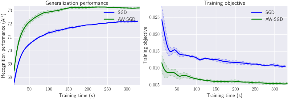
Figure 1 shows that AW-SGD converges faster than SGD for both training error and generalization performance. Acceleration is both in time and in iterations, and AW-SGD only costs per iteration with respect to SGD in our implementation. In further experiments, we noticed that the positive sampling bias parameter indeed gradually decreases, i.e. the /algorithm learns that it should focus more on the harder negative class. We also show that the values learned for this sampling parameter also depend on the category.
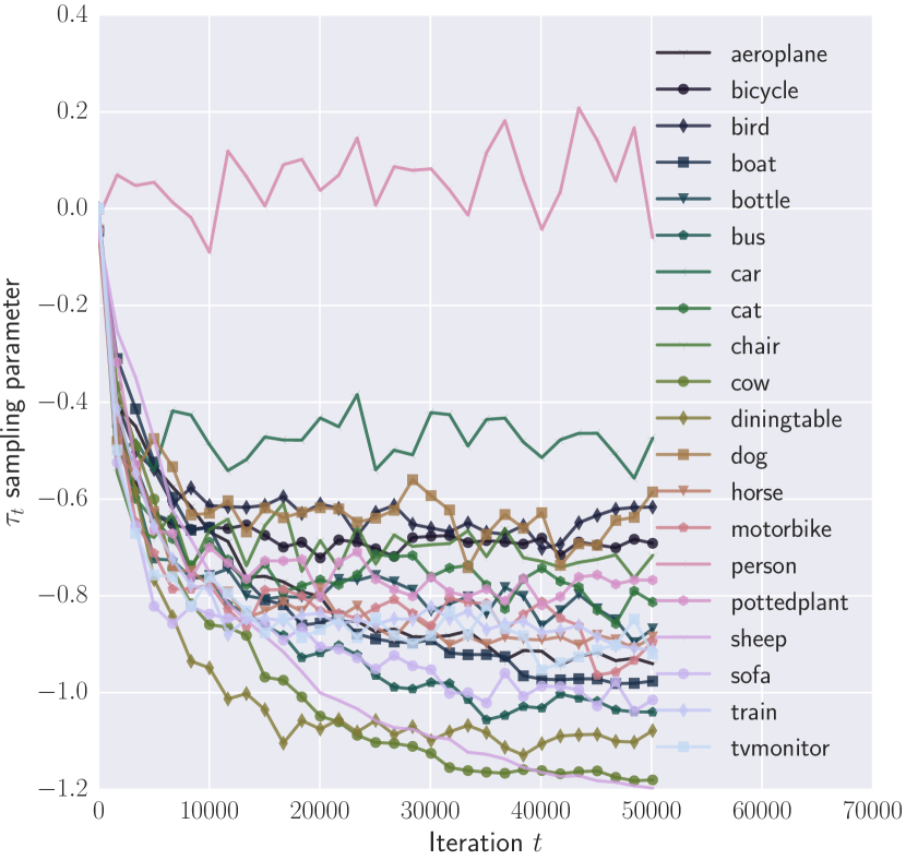
Figure 2 displays the evolution of the positive sampling bias parameter along AW-SGD iterations . Almost all classes expose the expected behavior of sampling more and more negatives as the optimization progresses, as the negatives correspond to anything but the object of interest, and are, therefore, much more varied and difficult to model. The “person” class is the only exception, because it is, by far, the category with the largest number of positives and intra-class variation. Note that, although the dynamics of the stochastic process are similar, the exact values obtained vary significantly depending on the class, which shows the self-tuning capacity of AW-SGD.
6 Application to Matrix factorization
We applied AW-SGD to learn how to sample the rows and columns in a SGD-based low-rank matrix decomposition algorithm. Let be a matrix that has been generated by a rank- matrix , where and . We consider a differentiable loss function where and is the observed value. With the squared loss, we have each entry of is a real scalar and . The full loss function is
| (16) |
We consider the sampling distributions over the set , where we independently sample a row and a column according to the discrete distributions and respectively, with , , , and . We define:
| (17) | ||||
| (18) |
with the softmax function. Using the square loss, as in the experiments below, the update equations in AW-SGD (Algo. 2) are:
| (19) |
| (20) | |||
| (21) |
| (22) | |||
| (23) |
where and , vectors with at index and respectively, and all other components are .
In the matrix factorization experiments, we used the mini-batch technique with batches of size 100, and were tuned to yield the minimum at convergence, separately with each algorithm. All results are averaged over 10 runs. and were initialized with zeros to get an initial uniform sampling distribution over the rows and columns. The model learning rate decrease was set to , was kept constant.
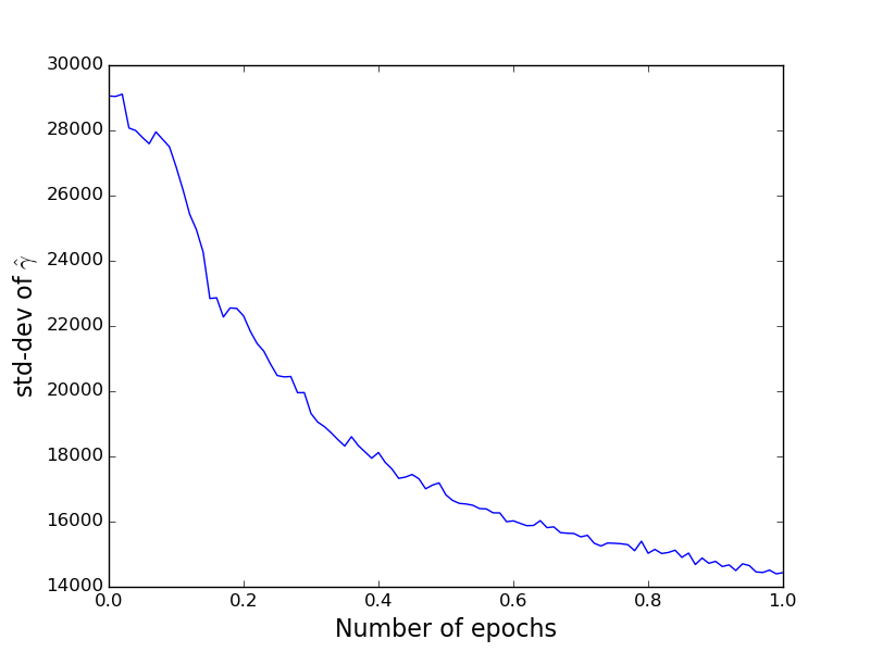
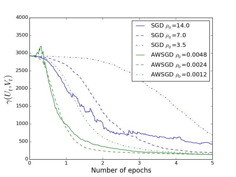
In Figure 3, we simulated a rank- matrix, for and , by sampling and using independent centered Gaussian variables with unit variance. To illustrate the benefit of adaptive sampling, we multiply by 100 a randomly drawn square block of size 20, to experimentally observe the benefit of a non uniform sampling strategy. The results of the minimal variance important sampling scheme (Algorithm 1) is shown on the left. We see that after having seen 50% of the number of matrix entries, the standard deviation of the importance sampling estimator is divided by two, meaning that we would need only half of the samples to evaluate the full loss compared to uniform sampling . Figure 4 shows the loss decrease of SGD and AW-SGD and on the same matrix for multiple learning rates. The axis is expressed in epochs, where one epoch corresponds to sampling of values in the matrix. AW-SGD converges significantly faster than the best uniformly sampled SGD, even after 1 epoch through the data. On average, AW-SGD requires half of the number of iterations to converge to the same value.
In-painting experiment
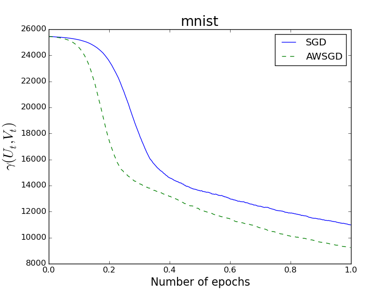
We compared both algorithms on the MNIST dataset [22], on which low-rank decomposition techniques have been successfully applied [23]. We factorized with the training set for the zero digit, a matrix, where each line is a image of a handwritten zero, and each column one pixel. Figure 5 shows the loss decrease for both algorithms on the first iteration. AW-SGD requires significantly less samples to reach the same error. At convergence, AW-SGD showed an average speedup in execution time compared to SGD, showing that its sampling choices compensate for its parametrization overhead.
Non-stationary data
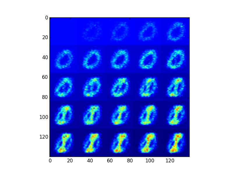
On Figure 6 we progressively substituted images of handwritten zeros by images of handwritten ones. It shows, every 2000 samples (i.e. 0.0005 epoch), the heatmap of the sampling probability of each pixel, , reorganized as grids. Substitution from zeros to ones was made between 10000 and 20000 samples (on 2nd line). One can distinctly recognize the zero digit first, that progressively fades out for the one digit222We created an animated gif with more of these images and inserted it in the supplementary material.. This transitions shows that AW-SGD learns to sample the digits that are likely to have a high impact on the loss. The algorithm adapts online to changes in the underlying distribution (transitions from one digit to another).
Combined with adaptive step size algorithms such as AdaGrad, we noticed that Adagrad did not improved the convergence speed of AW-SGD in our matrix factorization experiments. A possible explanation is that the adaptive sampling favors some rows and columns, and AdaGrad compensates the non-uniform sampling, such that using AW-SGD and AdaGrad simultaneously converges only slightly faster than AdaGrad alone. It should behave similarly on other parameterizations of where indices are linked to parameters indices. However, in many of our experiments, Adagrad performances were not matching the best cross-validated learning rates.
7 Sequential Control through Policy Gradient
Stochastic optimization is currently one of the most popular approaches for policy learning in the context of Markov Decision Processes. More precisely, policy gradient has become the method of choice in a large number of contexts in reinforcement learning [24; 25]. Here, optimizing the integral (1) is related to policy gradient algorithms which aim at minimizing an expected loss (i.e. a negative reward or a cost) or maximizing a reward in an episodic setting (i.e. with a predefined finite trajectory length) and off-policy estimation. Equivalently, if we consider the sampling space as being the (action, state) trajectory of a Markov Decision Process, AW-SGD can be viewed as a off-policy gradient algorithm, where and have the same parameterization, i.e. . The objective is to maximize the expected reward for the target policy , and to minimize the variance of the gradient for the policy gradient for the exploration policy .
We considered a canonical grid-world problem [26; 27] with a squared grid of size is considered. A classical reward setting has been applied: the reward function is a discounted instantaneous reward of assigned on each cell of the grid and a reward of for a terminal state located at the down right of the grid. In this context, an episode is considered as successful if the defined terminal state is reached. Finally, a random distribution of terminal states with a negative reward of are also positioned. The start state is located at the very up-left cell of the grid.
In this experimental setting, the parameters and of the target policy and the exploration policy are defined in the space . More precisely, the probability of an action at each position follows a multinomial distribution of parameters . Indeed, in the context of the grid type of environment that we will use in this section, these parameters basically correspond to the log-odds of the probability of moving in one of the four directions at each position of the grid (movements outside the grid do not change the position). The distribution of sampled trajectories are different from the distribution of trajectory derived from (off-policy learning).
The policy is optimized using Algorithm 2. The baseline corresponds to a policy iteration based on SGD where trajectories are sampled using their current policy estimate (on-policy learning). On Table 1, the table gives the average means and variances obtained for a batch of learning trials using both algorithms with properly tuned learning rate (the optimal learning rate is different in the two algorithms, for SGD and for AWSGD has been found). We can see that for all the tested grid sizes, there is a significant improvement (close to 10% relative improvement) of the expected success when adaptive weighted SGD is used instead of the on-policy learning SGD algorithm.
8 Adapting to Non-Uniform Architectures
In many large scale infrastructures, such as computation servers shared by many people, data access or gradient computation are unknown in advance. For example, in large scale image classification, some images might be stored in the RAM, leading to a access time that is order of times faster than other images stored only on the hard drive. These hardware systems are sometimes called Non-Uniform Memory Access [28]. It is also the case in matrix factorization, when some embeddings are stored locally, and others downloaded through the network. How can we inform the algorithm that it should sample more often data stored locally?
A simple modification of AW-SGD can enable the algorithm to adapt to non-uniform computation time. The key idea is to learn dynamically to minimize the expected loss decrease per unit of time. To make AW-SGD take into account this access time, we simply weighted the update of in Algorithm 2 by dividing it by the simulated access time to the sample . This is summarized in Algorithm 3.
As an experiment, we show in the matrix factorization case that the time-aware AW-SGD is able to learn and exploit the underlying hardware when the data does not fit entirely in memory, and one part of them has an extra access cost. To do so, we generate a rank- matrix, but without high variance block, so that variance is uniform across rows and columns. For the first half of the rows of the matrix, i.e. , we consider the data as being in main memory, and simulate an access cost of 100ns for each sampling in those rows, inspired by Jeff Dean’s explanations[29]. For the other half of the rows, , we multiply that access cost by a factor , we’ll call the slow block access factor. The simulated access time to the sample , is thus given by: if , and if . We ranged the factor from 2 to .
| AW-SGD | SGD | |
|---|---|---|
| 15 | ||
| 50 | ||
| 80 |
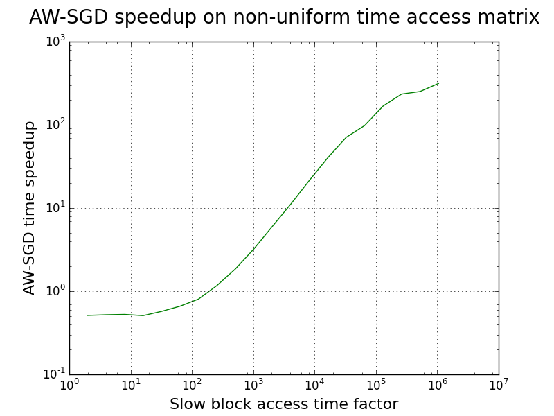
The time speedup achieved by the time-aware AW-SGD against SGD is plotted against the evolution of this factor in Figure 7. For each algorithm, we summed the real execution time and the simulated access times in order to take into account the time-aware AW-SGD sampling overhead. The speedup is computed after one epoch, by dividing SGD total time by AW-SGD total time. Positive speedups starts with a slow access time factor of roughly 200, which corresponds to a random read on a SSD. Below AW-SGD is slower, since the data is homogeneous, and time access difference is not yet big enough to compensate its overhead. At , corresponding to a read from another computer’s memory on local network, speedup reaches . At , a hard drive seek, AW-SGD is faster. This shows that the time-aware AW-SGD overhead is compensated by its sampling choices.
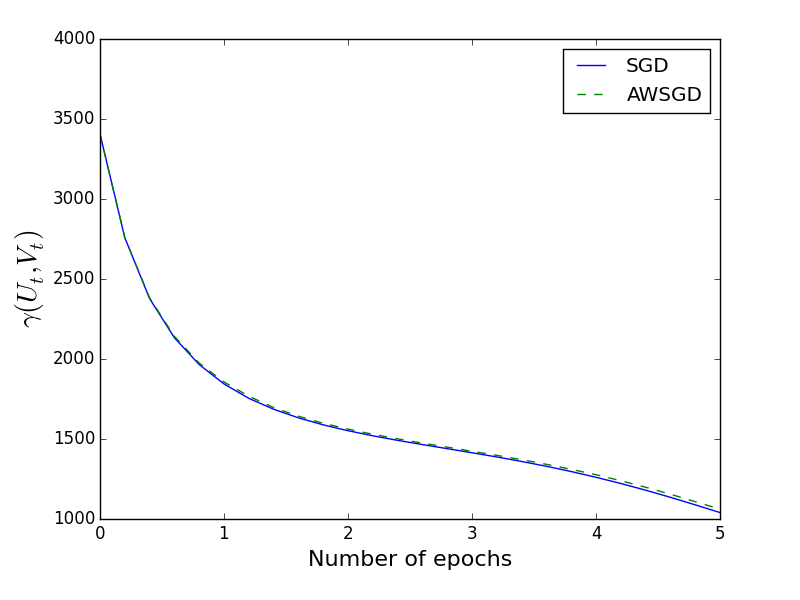
Figure 8 shows the loss decrease of both algorithms on the 5 first epochs with . It shows that if the access time was the uniform, AW-SGD would have the same convergence speed as standard SGD (this is expected by the design of this experiment). Hence, even in such case where there is no theoretical benefit of using the time-aware AW-SGD in terms of epochs, the fact that we learn the underlying access time to bias the sampling could potentially lead to huge improvements of the convergence time.
9 Conclusion
In this work, we argue that SGD and importance sampling can strongly benefit from each other. SGD algorithms can be used to learn the minimal variance sampling distribution, while importance sampling techniques can be used to improve the gradient estimation of SGD algorithm. We have introduced a simple yet efficient Adaptive Weighted SGD algorithm that can optimize a function while optimizing the way it samples the examples. We showed that this framework can be used in a large variety of problems, and experimented with it in three domains that have apparently no direct connections: image classification, matrix factorization and reinforcement learning. In all the cases, we can gain a significant speed-up by optimizing the way the samples are generated.
There are many more applications in which these variance reduction techniques have a strong potential. For example, in variational inference, the objective function is an integral and SGD algorithms are often used to increase convergence [30; 13]. Computing these integrals stochastically could be made more efficient by sampling non-uniformly in the integration space. Also, the estimation of intractable log-partition function, such as Boltzmann machines, are potential candidate models in which importance sampling has already been proposed, but without variance reduction technique [31].
This work also shows that we can learn about the algorithm while optimizing, as shown by the time-aware AW-SGD. This idea can be extended to design new types of meta-algorithms that learn to optimize or learn to coach other algorithms.
References
- [1] H. Robbins and S. Monro. A stochastic approximation method. Annals of Mathematical Statistics, 22(3), 1951.
- [2] L. Bottou. Online algorithms and stochastic approximations. In David Saad, editor, Online Learning and Neural Networks. Cambridge University Press, Cambridge, UK, 1998.
- [3] L Bottou and O Bousquet. The tradeoffs of large scale learning. In Suvrit Sra, Sebastian Nowozin, and Stephen J. Wright, editors, Optimization for Machine Learning, pages 351–368. MIT Press, 2011.
- [4] F Bach and E Moulines. Non-asymptotic analysis of stochastic approximation algorithms for machine learning. In NIPS, pages 451–459, 2011.
- [5] B. T. Polyak and A. B. Juditsky. Acceleration of stochastic approximation by averaging. SIAM Journal on Control and Optimization, 1992.
- [6] M Friedlander and M Schmidt. Hybrid deterministic-stochastic methods for data fitting. SIAM Journal on Scientific Computing, 2012.
- [7] J Duchi, E Hazan, and Y Singer. Adaptive subgradient methods for online learning and stochastic optimization. JMRL, 12:2121–2159, 2011.
- [8] Elad Hazan, Tomer Koren, and Nati Srebro. Beating sgd: Learning svms in sublinear time. In Advances in Neural Information Processing Systems, pages 1233–1241, 2011.
- [9] P Mineiro and N Karampatziakis. Loss-proportional subsampling for subsequent erm. In ICML, 2013.
- [10] J-S Senecal and Y Bengio. Adaptive importance sampling to accelerate training of a neural probabilistic language model. Technical report, IDIAP, 2003.
- [11] Yoshua Bengio and J-S Senecal. Adaptive importance sampling to accelerate training of a neural probabilistic language model. Neural Networks, IEEE Transactions on, 19(4):713–722, 2008.
- [12] SM Ross. Simulation academic press. San Diego, 1997.
- [13] J Paisley, D Blei, and M Jordan. Variational bayesian inference with stochastic search. ICML, 2012.
- [14] Yoshua Bengio, Jérôme Louradour, Ronan Collobert, and Jason Weston. Curriculum learning. In ICML ’09: Proceedings of the 26th Annual International Conference on Machine Learning, pages 41–48. ACM, 2009.
- [15] F Perronnin, Z Akata, Z Harchaoui, and C Schmid. Towards Good Practice in Large-Scale Learning for Image Classification. In CVPR, 2012.
- [16] N Dalal and W Triggs. Histograms of oriented gradients for human detection. In CVPR, 2005.
- [17] M Everingham, L Van Gool, C K I Williams, J Winn, and A Zisserman. The Pascal Visual Object Classes (VOC) Challenge. IJCV, 2010.
- [18] J Donahue, Y Jia, O Vinyals, J Hoffman, N Zhang, E Tzeng, and T Darrell. DeCAF : A Deep Convolutional Activation Feature for Generic Visual Recognition. In ICML, 2014.
- [19] M Oquab, L Bottou, I Laptev, and J Sivic. Learning and Transferring Mid-Level Image Representations using Convolutional Neural Networks. In CVPR, 2014.
- [20] R Girshick, J Donahue, T Darrell, and J Malik. Rich feature hierarchies for accurate object detection and semantic segmentation. In CVPR, 2014.
- [21] A Krizhevsky, GE Hinton, and I Sutskever. ImageNet Classification with Deep Convolutional Neural Networks. In NIPS, 2012.
- [22] Yann LeCun, Léon Bottou, Yoshua Bengio, and Patrick Haffner. Gradient-based learning applied to document recognition. Proceedings of the IEEE, 86(11):2278–2324, 1998.
- [23] Mithun Das Gupta and Jing Xiao. Non-negative matrix factorization as a feature selection tool for maximum margin classifiers. In Computer Vision and Pattern Recognition (CVPR), 2011 IEEE Conference on, pages 2841–2848. IEEE, 2011.
- [24] David Silver, Guy Lever, Nicolas Heess, Thomas Degris, Daan Wierstra, and Martin Riedmiller. Deterministic policy gradient algorithms. In ICML, volume 32 of JMLR Proceedings, pages 387–395, 2014.
- [25] Rémi Munos. Policy gradient in continuous time, May 2006.
- [26] Richard S. Sutton, editor. Reinforcement Learning, volume 173 of SECS. Kluwer Academic Publishers, 1992. Reprinted from volume 8(3–4) (1992) of Machine Learning.
- [27] C. Szepesvari. Algorithms for Reinforcement Learning. Synthesis lectures on artificial intelligence and machine learning. Morgan & Claypool, 2010.
- [28] Jaroslaw Nieplocha, Robert J Harrison, and Richard J Littlefield. Global arrays: A nonuniform memory access programming model for high-performance computers. The Journal of Supercomputing, 10(2):169–189, 1996.
- [29] J Dean. Software Engineering Advice from Building Large-Scale Distributed Systems. http://research.google.com/people/jeff/stanford-295-talk.pdf#13.
- [30] M Hoffman, D Blei, C Wang, and J Paisley. Stochastic variational inference. JMRL, 14(1):1303–1347, 2013.
- [31] R Salakhutdinov and I Murray. On the quantitative analysis of deep belief networks. In ICML, 2008.