Excitonic spectral features in strongly-coupled organic polaritons

Abstract

Starting from a microscopic model, we investigate the optical spectra of molecules in strongly-coupled organic microcavities examining how they might self-consistently adapt their coupling to light. We consider both rotational and vibrational degrees of freedom, focusing on features which can be seen in the peak in the center of the spectrum at the bare excitonic frequency. In both cases we find that the matter-light coupling can lead to a self-consistent change of the molecular states, with consequent temperature-dependent signatures in the absorption spectrum. However, for typical parameters, these effects are much too weak to explain recent measurements. We show that another mechanism which naturally arises from our model of vibrationally dressed polaritons has the right magnitude and temperature dependence to be at the origin of the observed data.

I Introduction

When matter is strongly coupled to light, the interaction cannot simply be thought of in terms of absorption and emission processes. Instead we must consider the eigenstates of the fully coupled matter-light system. The paradigmatic example of this is the existence of exciton polaritons, hybrid matter-light particles formed by the strong interaction between excitons and photons Hopfield (1958); Pekar (1958). Matter-light coupling can be engineered by confining light in optical cavities, so as to modify the density of states and the coupling to matter. For weak coupling, or a bad cavity, cavity losses are fast so one can eliminate virtual processes where photons are in the cavity. This gives Fermi’s golden rule, but with the cavity density of states modifying the emission rate, as first discussed by Purcell Purcell (1946). When coupling is strong, first order perturbation theory (i.e. Fermi’s golden rule) fails, as there can instead be coherent emission and reabsorption of photons before light leaks out of the cavity Björk et al. (1991); Weisbuch et al. (1992).

A natural context in which strong matter-light coupling arises is between organic molecules and light in semiconductor microcavities. Because of the existence of conjugated $\pi$ bonds in organic molecules, electronic transitions can acquire large dipole moments Agranovich (1968); Davydov (1971); Agranovich (2009), leading to very strong coupling to light. When such molecules are placed in optical microcavities this leads to huge polariton splittings Lidzey et al. (1998, 1999); Schwartz et al. (2011); Tischler et al. (2005). These scales allow such experiments to be performed at room temperature, whereas for many inorganic materials, cryogenic temperatures are required. The polariton splitting is due to a collective phenomenon: the electronic transitions of many molecules couple to radiation, and as such the polariton splitting grows as the square root of the molecule density. In contrast, in weak coupling, the rate at which one molecule emits is independent of whether or not any other molecules are present Dicke (1954).

Much of the recent work on organic microcavity polaritons (see, e.g. Ref. Michetti et al. (2015) for a recent review) has been focused on condensation and lasing Kéna-Cohen et al. (2008); Kéna-Cohen and Forrest (2010); Plumhof et al. (2014); Daskalakis et al. (2014), involving a strongly pumped system, and the appearance of macroscopic quantum coherence. There has however also been significant recent work on the effects of matter-light coupling in the vacuum state, i.e. without strong pumping. Such work aims to understand how the physical and chemical properties of organic molecules are affected by strong coupling to electromagnetic modes. Examples of this include modifying the rates of photochemical reactions Hutchison et al. (2012), or modifying the transport properties of organic semiconductors Orgiu et al. (2015); Schachenmayer et al. (2014); Feist and Garcia-Vidal (2015). More recently, there has also been experimental Shalabney et al. (2015) and theoretical Roelli et al. (2014); Pino et al. (2015, 2015) work on coupling the vibrational state of organic molecules to infra-red radiation, leading to molecular optomechanics. Theoretical work Spano (2015) has also studied how strong matter-light coupling to electronic states can suppress the effects of disorder and vibronic features in the polariton spectrum. Of particular interest for the present paper is a recent work from the Ebbesen group Canaguier-Durand et al. (2013), in which the optical spectra of strongly-coupled organic microcavities were studied by varying molecular concentration and temperature, and paying particular attention to the relative weights of the resonant features in the absorption spectra: the two polariton peaks, and a third peak at the bare excitonic energy Schwartz et al. (2013).

Our aim in this manuscript is to examine the behavior of such strongly-coupled organic microcavities starting from various microscopic models, allowing quantitative predictions of the extent to which a self-consistent adaptation of the molecular state, driven by coupling with light, may occur.

To understand the variation of the optical spectra with both concentration and temperature the models which we consider all contain a variable degree of coupling to light. This is because a molecule that has strictly zero coupling to light is not visible in the absorption spectrum, while molecules with a small but non-zero coupling will lead to absorption at the bare molecular energy. In order that the coupling to light can vary self consistently (in response to the Rabi splitting), it must depend on some adaptable feature of the state or environment of the molecule. i.e. there must be some physical property that can vary, which determines the strength of matter-light coupling. We refer to this concept hereafter as “self-consistent molecular adaptation”. We refer to this process as “self-consistent” because the effective matter-light coupling depends on (some aspect of) the molecular state, and the molecular state is modified because of how its energy depends on the matter-light coupling. In the first part of this manuscript we investigate in detail two candidates that could lead to self-consistent adaptation: rotational and vibrational degrees of freedom, we also consider an extension of these models to generic (classical) aspects of the molecules physical or chemical state. While we do find a temperature dependence of the optical spectra, the involved energy scales turn out to be incompatible with the observation of Ref. Canaguier-Durand et al. (2013). In the final part of the present work, we examine how our model of vibrationally dressed polaritons naturally predicts an effect whose energy scale is of the right magnitude to explain the data. This effect does not involve the renormalization of the coupling strength, but instead involves the effect of vibrational replicas and their coupling to the excitonic transition on the optical spectra. Our results thus show a first example of the rich, and presently poorly understood behavior that can stem from the interplay of strong matter-light coupling with strong coupling to vibrational/conformational modes of the molecules.

We start by noting that the existence of a peak at the bare energy of the exciton, brought forward as evidence of novel physics in Ref. Canaguier-Durand et al. (2013), is not unexpected; such a “residual excitonic peak” has been seen in many cases, for example Ref. Houdré et al. (1996) discussed theoretically, and demonstrated experimentally, the appearance of such a feature in a GaAs/AlGaAs heterostructure, containing quantum wells inside a DBR microcavity. While such a peak comes from the spectral weight of the exciton line, it is important to note that this peak cannot be viewed simply as excitons which do not couple to light: if they did not couple, they would not be visible in the absorption or transmission spectrum. The origin of the peak can be understood physically as coming from the subradiant excitonic states due to inhomogeneous broadening. In a disordered system, the coupling to the photon mode picks out a specific superradiant state, which forms the polaritons, while the other states — orthogonal to this superradiant state — remain at the bare exciton energies. However, because of energetic disorder, the superradiant state is not an energy eigenstate, and a residual coupling between the superradiant and subradiant states exists, so that the spectral weight of the subradiant states is visible in the optical spectrum Houdré et al. (1996); Eastham and Littlewood (2001); Keeling et al. (2005).

A simple analytical treatment shows that the weight of this residual excitonic peak does decrease as the matter-light coupling increases. The existence of this peak is thus consistent with the behavior seen in Canaguier-Durand et al. (2013). However, on its own this explanation cannot account for the temperature dependence observed, as the residual excitonic peak should be unaffected by temperature, unless $k_{B}T$ approaches optical energies, of the order of $1\text{eV}$ (for comparison 300K$\approx 25$meV). One of the main goals of this paper is to address how this temperature dependence may occur.

As will become clear in the following, to discuss the microscopic theory of such effects, it will be crucial to consider the physics of ultrastrong matter-light coupling Ciuti et al. (2005); De Liberato (2015), and the breakdown of the rotating wave approximation (RWA). This requires retaining “counter-rotating” terms in the matter-light coupling Hamiltonian. These terms, which involve simultaneous creation of pairs of excitations, are typically considered to be non-resonant and so are often neglected. However, if the matter-light coupling is a significant fraction of the bare exciton and photon energies, then these terms have a non-negligible impact. Such behavior has been seen in both inorganic Anappara et al. (2009) and organic Schwartz et al. (2011); Gambino et al. (2014); Gubbin et al. (2014) systems, with a current record of a coupling strength $87\%$ of the bare oscillator frequency Maissen et al. (2014). Our focus in this paper is on the more typical regime where such counter-rotating terms cannot be neglected, but remain sufficiently small to be treated perturbatively.

The rest of the paper is structured in two main sections. In section II we consider how temperature dependence can arise due to self-consistent adaptation of the rotational and vibrational degrees of freedom of the molecules, via a mechanism very similar to that proposed in Ref. Canaguier-Durand et al. (2013). For the orientational degree of freedom, we consider both free molecules, and molecules with randomly pinned orientations as appropriate in a polymer matrix. We will see that in such systems we do predict a temperature dependence of the residual excitonic peak. However, while this effect could potentially be observed in other experimental realizations, the energy scales (temperatures) required and the scaling with molecular concentration are not compatible with the experimental observations reported in Ref. Canaguier-Durand et al. (2013).

In section III we instead consider a different effect, arising from the interplay of vibrational modes with the matter-light coupling, which is able to reproduce similar behavior to that observed in experiments. Specifically we find that vibrational excitations dress the residual excitonic peak in a strongly temperature dependent manner. Moreover, the form of the vibrational dressed spectrum shows that the spectral feature at the exciton energy can have a more complex interpretation than that previously considered Houdré et al. (1996).

A brief but self-contained account of the main theoretical methods used throughout this paper is given in the appendices.

II Self-consistent molecular adaptation due to strong coupling

In this section we consider whether self-consistent molecular adaptation can enhance matter-light coupling by renormalizing the bare matter-light coupling strength. We consider models in which the effective matter-light coupling strength of a given molecule depends on the configuration of that molecule, such as its orientation, or its vibrational state. We then ask how this same matter-light coupling modifies the energy landscape for the auxiliary parameters describing the configuration. This leads to the idea of self consistency — if strong coupling leads to a reduction of the ground state energy, the energy landscape is deformed so as to favor auxiliary parameters for which the effective matter-light coupling is as large as possible. Our aim is to derive this from a microscopic model, and so quantify this effect. In the following we consider two potential scenarios involving adaptation of either orientational or vibrational degrees of freedom.

If such a self-consistent enhancement of matter-light coupling occurs, then this can lead to a temperature dependent effective coupling, and thus to a temperature dependence of the residual excitonic peak. We show that such an effect exists, but that its strength is relatively weak, and that the relevant energy scale shows no collective enhancement, i.e. the presence of $N_{m}$ molecules does not lead to a $N_{m}$ enhancement of this energy scale, because it must compete with the extensive entropy gain from orientational or vibrational disorder. As such, while increasing the molecular concentration will increase the polariton splitting, it has little effect on the self-consistent orientation. Changing the bare oscillator strength of the molecules does however affect both the polariton splitting and the self-consistent molecular adaptation energy scale.

Before introducing any auxiliary variables, the basic Hamiltonian which we consider is an extended Dicke model, including diamagnetic terms:

$$\hat{H}=\sum_{\mathbf{k}}\omega_{\mathbf{k}}\hat{\psi}^{\dagger}_{\mathbf{k}}\hat{\psi}_{\mathbf{k}}+\sum_{n}\Biggl{[}\frac{\epsilon_{n}}{2}\sigma_{n}^{z}\\ +\sum_{\mathbf{k}}g_{\mathbf{k},n}\varphi_{\mathbf{k}}(\mathbf{r}_{n})\sigma^{x}_{n}+\left(\sum_{\mathbf{k}}\sqrt{D_{\mathbf{k}}}\varphi_{\mathbf{k}}(\mathbf{r}_{n})\right)^{2}\Biggr{]},$$ (1)

where the field $\varphi_{\mathbf{k}}(\mathbf{r})=\hat{\psi}^{\dagger}_{\mathbf{k}}e^{-i\mathbf{k}\cdot\mathbf{r}}+\hat{\psi}_{\mathbf{k}}e^{i\mathbf{k}\cdot\mathbf{r}}$ is written in terms of the bosonic creation and annihilation operators $\hat{\psi}_{\mathbf{k}},\hat{\psi}^{\dagger}_{\mathbf{k}}$ describing photon modes labeled by their in-plane momentum $\mathbf{k}$, and energy $\omega_{\mathbf{k}}$. The Pauli matrices $\sigma^{i=x,y,z}_{n}$ describe the electronic state of the molecules. For completeness, we therefore also included the diamagnetic terms, arising from the $\mathbf{A}^{2}$ term of the minimal coupling Hamiltonian De Liberato (2014).

Furthermore, in order to consider varying the cavity mode volume while respecting the Thomas-Reiche-Kuhn sum rule Rzazewski et al. (1975) we use $g_{\mathbf{k},n}=\sqrt{\epsilon_{n}D_{\mathbf{k}}f_{n}}$ where $0<f_{n}<1$ is the oscillator strength of the given molecule. The coefficient $D_{\mathbf{k}}$ depends on the electric field strength of a single photon, and the properties of the effective charges that respond to the field.

If we assume an uniform distribution of molecules, momentum conservation can be used to write the diamagnetic term in Eq. (1) as $N_{m}\sum_{k}D_{\mathbf{k}}(\hat{\psi}^{\dagger}_{\mathbf{k}}+\hat{\psi}_{-\mathbf{k}})(\hat{\psi}^{\dagger}_{-\mathbf{k}}+\hat{\psi}_{\mathbf{k}})$. This term can then be removed by a Bogoliubov transformation $\hat{\psi}_{\mathbf{k}}\to\cosh\theta_{\mathbf{k}}\hat{\psi}_{\mathbf{k}}+\sinh\theta_{\mathbf{k}}\hat{\psi}^{\dagger}_{\mathbf{k}}$, yielding the effective Hamiltonian:

$$\hat{H}=\sum_{\mathbf{k}}\tilde{\omega}_{\mathbf{k}}\hat{\psi}^{\dagger}_{\mathbf{k}}\hat{\psi}_{\mathbf{k}}+\sum_{n}\hat{h}_{n},$$ (2)

where the on-site Hamiltonian is given by

$$\hat{h}_{n}=\frac{\epsilon_{n}}{2}\sigma_{n}^{z}+\sum_{\mathbf{k}}\tilde{g}_{\mathbf{k},n}\varphi(\mathbf{r}_{n})\sigma^{x}_{n},$$ (3)

and the renormalized parameters $\tilde{\omega}_{\mathbf{k}},\tilde{g}_{\mathbf{k}}$ are:

$$\tilde{\omega}_{\mathbf{k}}=\sqrt{\omega_{\mathbf{k}}(\omega_{\mathbf{k}}+4N_{m}D_{\mathbf{k}})},\qquad\tilde{g}_{\mathbf{k},n}=g_{\mathbf{k},n}\sqrt{\frac{\omega_{k}}{\tilde{\omega}_{k}}},$$ (4)

with $N_{m}$ the number of molecules in the mode volume.

In the dipole approximation, for a molecule with a single mobile electron $D_{\mathbf{k}}=\zeta/\omega_{\mathbf{k}}V$ with $V$ the mode volume and $\zeta=\hbar^{2}e^{2}/(4m_{r}\varepsilon_{0})$ quantifying the electronic response of a single electron in terms of the vacuum permittivity $\varepsilon_{0}$ and its reduced mass $m_{r}$. For molecules involving many conjugated bonds, the coefficient $\zeta$ is replaced by a sum over all mobile charges. It is important to note that changing the cavity length changes both the mode volume $V$ (and hence both $D_{\mathbf{k}}$ and $g_{\mathbf{k},n}$) and the spectrum of photon modes $\omega_{\mathbf{k}}$. In the following numerical results we will fix the values of the polariton splitting $g_{\mathbf{k},n}\sqrt{N_{m}}$, exciton energy $\epsilon_{n}$, and coupling strength $f$, and use these to determine $D_{\mathbf{k}}N_{m}$.

Before considering the role of vibrational and orientational degrees of freedom, we consider how the existence of a temperature dependent matter-light coupling strength, $\tilde{g}_{\text{eff},\mathbf{k},n}$ would be seen in the absorption spectrum. For this purpose, it is sufficient to consider the absorption spectrum of Eq. (2), and its dependence on $\tilde{g}_{\mathbf{k},n}$. Appendix A summarizes how the absorption spectrum can be calculated, including the counter-rotating terms in the matter-light coupling Ciuti and Carusotto (2006). In performing these calculations, as noted above, it is necessary to include disorder in order to see the residual excitonic feature. We will consider disorder in the exciton energies, denoted by the energy distribution $h(\epsilon)$ For simplicity we consider only disorder in the energies and we ignore the subleading effect of the exciton energy distribution on the coupling strength $g_{\mathbf{k},n}$, by using the averaged value $g_{\mathbf{k}}^{2}\equiv\sum_{n}g_{\mathbf{k},n}^{2}/N_{m}$. As discussed in the appendix, we consider the quantity $a_{\mathbf{k}}(\nu)=-2\Im[G^{R}_{\mathbf{k},xx}(\nu)]$, in terms of the retarded Green’s $G^{R}_{\mathbf{k},xx}(\nu)$, which is proportional to the absorption spectrum for a good cavity. The Green’s function has the form:

$${G}^{R}_{\mathbf{k},xx}(\nu)=\frac{2{\omega}_{k}}{\nu^{2}-\tilde{\omega}_{k}^{2}+2{\omega}_{k}\Sigma_{\mathbf{k},xx}(\nu)+i\tilde{\omega}_{k}\tilde{\kappa}(\nu)},$$ (5)

where the excitonic self energy for Eq. (2), can be written as ${\Sigma}_{\mathbf{k},xx}={\Sigma}^{\text{RWA}}_{\mathbf{k},+-}(\nu)+{\Sigma}^{\text{RWA}}_{\mathbf{k},+-}(-\nu)^{\ast}$ with:

$${\Sigma}^{\text{RWA}}_{\mathbf{k},+-}(\nu)=-g^{2}_{\mathbf{k}}N_{m}\int_{-\infty}^{\infty}\!\!\!\!d\epsilon h(\epsilon)\frac{\tanh(\beta\epsilon/2)}{\nu+i\gamma^{+}-\epsilon}.$$ (6)

Here $\beta=(k_{B}T)^{-1}$ is the inverse temperature and $\gamma$ is the homogeneous linewidth of the excitons. In the following we will present results both for $\gamma=0^{+}$ and for small but non-zero $\gamma$ as indicated in the figure captions.

The spectrum is shown in Fig. 1, focusing on the residual excitonic peak, to show its dependence on the polariton splitting. As noted above, such a feature has been observed and commented on several times before, e.g. Houdré et al. (1996); Eastham and Littlewood (2001); Keeling et al. (2005). When the polariton splitting $g\sqrt{N_{m}}$ is increased, the splitting between the lower and upper polaritons increases, and the exciton spectral weight of the feature at the exciton energy decreases. The asymmetry between the shift of the lower and upper polaritons arises due to the diamagnetic term $D_{k}$ renormalizing the photon energy. If the coupling to light is weak, so that the RWA is valid, this asymmetry vanishes. In Fig. 1 (b) we show how the spectrum is modified by including the effects of cavity losses and non-radiative excitonic decay as described in Appendix A. The main effect these processes have is to broaden and thus reduce the height of the polariton peaks, there is also additional broadening to the central peak.

Because the only temperature dependence of Eq. (5,6) is via the combination $\tanh(\beta\epsilon/2)$, the spectrum is temperature independent while $k_{B}T\ll\epsilon$ (with $\epsilon$ of the order of the exciton bare energy). Therefore, as noted in the introduction, the experimentally observed temperature dependence cannot occur from this mechanism alone, unless the effective value of $g_{\mathbf{k},n}$ is made temperature dependent via its dependence on configuration. We now go on to consider if this effect is plausible.

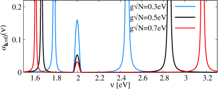
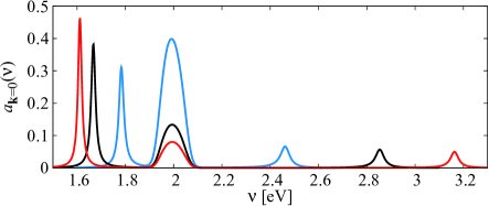
Figure 1: (color online) Evolution of $\mathbf{k}=0$ absorption spectrum, $a(\nu)$ vs polariton splitting $g_{\mathbf{k}=0}\sqrt{N_{m}}$ for the system with no auxiliary degrees of freedom. Plotted for $k_{B}T=0.025$eV (i.e. $T=290$K), $f=0.05,\omega_{\mathbf{k}=0}=2.1$eV, and a truncated Gaussian distribution $h(\epsilon)\propto\Theta(\epsilon)e^{(\epsilon-\epsilon_{0})^{2}/2\sigma^{2}}$ with $\epsilon_{0}=2.0$eV, $\sigma=0.01$eV. Panel (a) shows the results with a perfect cavity while (b) includes the effects of cavity losses at rate $\kappa=0.075$eV and excitonic non-radiative decay at rate $\gamma=10^{-4}$eV also the width of the energy distribution is larger, $\sigma=0.025$eV as discussed in Appendix A.

To consider molecular adaptation, the Hamiltonian in Eq. (2) will be modified to include either orientational or vibrational degrees of freedom. These are illustrated in Fig. 2. We next introduce these modifications and then discuss how they may be treated.

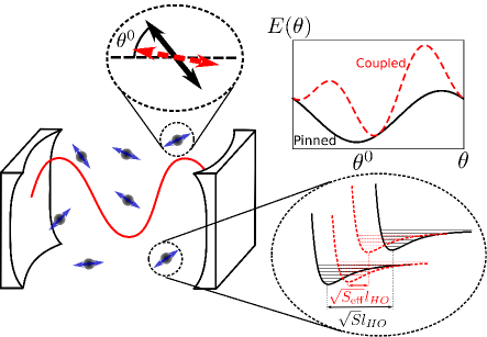
Figure 2: (color online) Schematic diagram showing orientational and vibrational degrees of freedom. The top right inset shows the potential energy landscape with (dashed red line) and without (solid black line) a cavity. The other insets show (top) the orientational degree of freedom and (bottom-right) the vibrational degree of freedom illustrating how the coupling to light decreases the displacement between the ground and excited manifolds. Shifts due to coupling to the cavity are exaggerated for clarity in all three insets.

The Hamiltonian including an orientational degree of freedom takes the same form as Eq. (2) with the on-site part

$$\hat{h}_{n} =\frac{\epsilon_{n}}{2}\sigma_{n}^{z}+\Lambda_{n}(\theta_{n})+\sum_{\mathbf{k}}\tilde{g}_{\mathbf{k},n}\cos(\theta_{n})\varphi_{\mathbf{k}}(\mathbf{r}_{n})\sigma^{x}_{n},$$ (7)

where the angle $\theta_{n}$ parametrizes the orientation of the dipole moment of the $n$th molecule with respect to the polarization of the cavity electric field, thus reducing the oscillator strength. The term $\Lambda_{n}(\theta_{n})$ represents the bare dependence of the Hamiltonian on orientation. This term allows one to model pinning of the orientation $\theta_{n}$. For simplicity we consider only a classical orientational degree of freedom; the corresponding quantum theory would require us to also include a rotational kinetic energy term, and diagonalize the resulting Hamiltonian. The effective matter-light coupling strength, which depends on the distribution of angles $\theta_{n}$ adopted by the molecule, can be written as $\tilde{g}^{2}_{\mathbf{k},n,\text{eff}}=\tilde{g}^{2}_{\mathbf{k},n}\langle\langle\cos^{2}(\theta_{n})\rangle\rangle$, where the double angle brackets represent both an ensemble and thermal average.

To consider vibrational degrees of freedom, we again start from the transformed Hamiltonian, Eq. (2), and now consider the following modification:

$$\hat{h}_{n}=\frac{\epsilon_{n}}{2}\sigma_{n}^{z}+\sum_{\mathbf{k}}\tilde{g}_{\mathbf{k},n}\varphi_{\mathbf{k}}(\mathbf{r}_{n})\sigma^{x}_{n}+\\ \sum_{m}\Omega_{m}\left(\hat{b}^{\dagger}_{n,m}\hat{b}_{n,m}+\frac{\sqrt{S_{m}}}{2}(\hat{b}^{\dagger}_{n,m}+\hat{b}_{n,m})\sigma^{z}_{n}\right).$$ (8)

Here $\hat{b}_{n,m},\hat{b}^{\dagger}_{n,m}$ describe the $m$th harmonic vibrational mode of molecule $n$, with the mode having frequency $\Omega_{m}$ and its coupling to the electronic state being parametrized by the Huang-Rhys parameter $\sqrt{S_{m}}$. In this case, defining the effective oscillator strength is more involved: the effective oscillator strength depends on the matrix element describing the overlap between the vibrational states in the ground and excited state manifold. We return to this point in later sections.

For both the orientational and vibrational degrees of freedom, our aim is to find how the matter-light coupling is self-consistently modified by these auxiliary degrees of freedom: i.e. how the presence of matter-light coupling modifies the distribution of orientational or vibrational states, and how this in turn affects the effective matter-light coupling strength. We consider a case without any strong pumping, and with a temperature such that $k_{B}T\ll\omega,\epsilon$, which is typically satisfied even at room temperature for organic polaritons. As such, the origin of the “self-consistent” dependence of configuration on the matter-light coupling coupling arises due to the existence of the counter-rotating terms in the original Hamiltonian: If these terms were neglected then the energy in the ground state sector can be trivially found as the ground state would correspond to the empty state, and its energy would therefore not involve the matter-light coupling strength at all Ciuti et al. (2005). The presence of counter-rotating terms means that the ground state sector also involves an admixture of all even parity sectors, and the degree of admixture depends on the effective matter-light coupling.

As discussed below, while exact solutions are possible in some limiting cases of the orientational problem, these are not generally possible at finite temperature, nor for the vibrational problem. This is because thermal or quantum fluctuations of the auxiliary degrees of freedom break translational symmetry, preventing simple exact diagonalization. As such, we proceed using the Schrieffer-Wolff formalism Schrieffer and Wolff (1966), which allows us to consider perturbatively the effects of these counter-rotating terms, and how they modify the energy landscape seen by the auxiliary orientational or vibrational degrees of freedom. For completeness, appendix B provides a brief summary of the Schrieffer-Wolff formalism. The essential point is to separate $\hat{H}=\hat{H}_{0}+\hat{H}_{1}$, where $\hat{H}_{1}$ are the terms treated perturbatively. At leading order this gives an effective Hamiltonian:

$$\hat{\tilde{H}}\approx\hat{H}_{0}+\frac{i}{2}\left[\hat{G},\hat{H}_{1}\right],\quad\hat{G}:\ [\hat{G},\hat{H}_{0}]\equiv i\hat{H}_{1}.$$ (9)

Taking the counter-rotating terms as $\hat{H}_{1}$, the perturbation theory is controlled by the small parameter $\tilde{g}_{\mathbf{k},n}/(\omega_{\mathbf{k}}+\epsilon_{n})$, which is indeed small for the physical parameters we consider . We are thus in a regime where the counter-rotating terms cannot be ignored, but where they can be included perturbatively. In the following sections we apply this approach in turn to the orientational and vibrational degrees of freedom, and see how the effective matter-light coupling can be derived self-consistently.

II.1 Orientational degrees of freedom

As discussed above, we consider first the classical orientational degrees of freedom $\theta_{n}$, subject to a pinning potential $\Lambda_{n}(\theta_{n})$. If all molecules are identical, $\Lambda_{n}(\theta_{n})=\Lambda(\theta_{n})$, then one can find the zero temperature ground state by choosing $\theta_{n}=\theta$. For the ground state, all that is required is to find the quantum ground state of Eq. (7) as a function of $\theta$ and then minimize over $\theta$. Since Eq. (7) is translationally invariant in the case $\theta_{n}=\theta$, it is possible to find the exact ground state in the bosonic approximation by Fourier transforming. The bosonic approximation assumes the occupation of each excited molecule is small, a result that is valid unless $g_{\mathbf{k}}\gg\omega_{\mathbf{k}},\epsilon$ Casanova et al. (2010); De Liberato (2014). However, at finite temperature, even for identical molecules, it is crucial to allow independent fluctuations of each $\theta_{n}$; assuming $\theta_{n}=\theta$ massively underestimates the entropy at finite temperature. At zero temperature, one may compare the exact solution to the Schrieffer-Wolff perturbative expansion used below, and one finds that these indeed match to leading order.

For this rotational case, the form of $\hat{G}$ required in Eq. (9) can be found trivially, and the resulting Hamiltonian can most conveniently be written as $\hat{\tilde{H}}=\sum_{\mathbf{k}}\tilde{\omega}_{\mathbf{k}}\hat{\psi}^{\dagger}_{\mathbf{k}}\hat{\psi}_{\mathbf{k}}+\sum_{n}\hat{\tilde{h}}_{n}$, with the molecular Hamiltonian in the form:

$$\hat{\tilde{h}}_{n}={\hat{h}}^{(0,\text{RWA})}_{n}-\sum_{\mathbf{k}}\frac{\tilde{g}_{\mathbf{k},n}^{2}\cos^{2}(\theta_{n})}{\tilde{\omega}_{\mathbf{k}}+\epsilon_{n}},$$

where ${\hat{h}}^{(0,\text{RWA})}_{n}$ is the bare molecular Hamiltonian, including the RWA coupling to light and including the pinning term $\Lambda_{n}(\theta_{n})$.

In order to consider the thermal distribution of $\theta_{n}$, we must specify the orientational potential $\Lambda_{n}(\theta_{n})$. We consider a form

$$\Lambda_{n}(\theta_{n})=\lambda\sin^{2}\left(\frac{\theta_{n}-\theta_{n}^{0}}{2}\right),$$ (10)

which tries to pin the molecules at angle $\theta_{n}^{0}$, relative to the cavity electric field, with strength $\lambda$. We may thus consider both the free orientation case, $\lambda=0$, and the pinned case simultaneously. In what follows we will assume that the pinning angles have a uniform distribution such as would be found in a polymer matrix. This treatment, however, ignores effects which would be important in systems such as organic crystals in which the pinning angle has a fixed direction. The energy landscape for each angle $\theta_{n}$, given the pinning angle $\theta_{n}^{0}$ is then:

$$E(\theta_{n}|\theta_{n}^{0})=\lambda\sin^{2}\left(\frac{\theta_{n}-\theta_{n}^{0}}{2}\right)-\sum_{\mathbf{k}}\frac{\tilde{g}_{\mathbf{k}}^{2}\cos^{2}(\theta_{n})}{\tilde{\omega}_{\mathbf{k}}+\epsilon}.$$ (11)

where for simplicity we have assumed that each molecule has the same values of $\epsilon,\tilde{g}_{\mathbf{k}}$ and the only disorder is in the pinning angles. In the following we will define the quantity:

$$K_{0}\equiv\sum_{\mathbf{k}}\frac{\tilde{g}_{\mathbf{k}}^{2}}{(\tilde{\omega}_{\mathbf{k}}+\epsilon)}.$$ (12)

The quantity $K_{0}$ characterizes the self-consistent energy favoring alignment of molecules. Replacing the summation by an integral, and inserting the explicit forms of $g_{\mathbf{k}}$ and $D_{\mathbf{k}}$ written above we have that

$$K_{0}=\frac{f\epsilon\zeta}{l_{c}}\int_{0}^{\Lambda}\frac{kdk}{(2\pi)}\frac{1}{\tilde{\omega}_{k}(\tilde{\omega}_{k}+\epsilon)},$$ (13)

where $l_{c}$ is again the cavity length, $\zeta$ the combination defined following Eq. (2), and $\Lambda=2\pi/a_{\text{Bohr}}$ is a cutoff reflecting the breakdown of the dipole approximation. To evaluate such integrals it is useful to write the dispersion in the form $\tilde{\omega}_{k}^{2}=(\omega_{0}^{2}+c^{2}k^{2})+4\zeta N_{m}/V$ which allows us to find the exact result

$$K_{0}=\frac{f\epsilon\zeta}{2\pi l_{c}c^{2}}\ln\left(\frac{\epsilon+\tilde{\omega}_{\Lambda}}{\epsilon+\tilde{\omega}_{0}}\right).$$ (14)

A notable feature of Eq. (14), as anticipated above, is that this quantity does not simply increase as one increases the polariton splitting by varying the density of emitters, $N_{m}/V$. There is a sub-leading dependence on the molecule density, via the renormalization $\omega_{\mathbf{k}}\to\tilde{\omega}_{\mathbf{k}}$ given in Eq. (4). However this effect is only significant in the deep strong coupling limit Casanova et al. (2010); De Liberato (2014). Physically this lack of scaling with $N_{m}$ is because this “molecular adaptation energy” depends on the shift seen for each molecule. Inserting typical experimental values for an organic system $N_{m}/V=4.2\cdot 10^{25}\text{m}^{-3}$, $\epsilon=\omega_{0}=2.1$eV, $l_{c}=145$nm, $f=0.5$, $a_{\text{Bohr}}=2$nm, $\zeta=4.3$eV²nm³ which correspond to the values extracted from Ref. Canaguier-Durand et al. (2013), one finds that

$$K_{0}=6.3\cdot 10^{-4}\text{meV},$$

which is much smaller than $k_{B}T$ at room temperature.

As noted earlier, the effective matter-light coupling strength is given by ${g_{\text{eff},\mathbf{k}}^{2}}={g^{2}_{\mathbf{k}}}\langle\langle\cos^{2}(\theta_{n})\rangle\rangle.$ At zero temperature, this corresponds to minimizing the energy, leading to $\lambda_{n}\sin(\theta_{n}-\theta_{n}^{0})=-2K_{0}\sin(2\theta_{n})$. However, since the value of $K_{0}$ given above is such that $K_{0}\ll k_{B}T$, it is crucial to consider finite temperatures. The smallness of the ratio $K_{0}/k_{B}T$ will also allow us to make further perturbative expansions in the following.

Defining ${g^{2}_{\text{eff}}}/{g^{2}}\equiv\langle\langle\cos^{2}(\theta_{n})\rangle\rangle$, this ratio can be calculated as

$$\frac{g_{\text{eff}}^{2}}{g^{2}}=\frac{1}{2\pi\beta}\frac{d}{dK_{0}}\int d\theta^{0}\ln[\mathcal{Z}(\lambda,K_{0},\theta^{0})],$$ (15)

where the partition function is

$$\mathcal{Z}(\lambda,K_{0},\theta^{0})=\!\!\int\!\!d\theta\exp\left[\beta K_{0}\cos^{2}\theta-\beta\lambda\sin^{2}\left(\frac{\theta-\theta^{0}}{2}\right)\right].$$

As noted above $\beta K_{0}\ll 1$, and so we may Taylor expand in this small parameter to get a closed form for $g_{\text{eff}}$. Assuming that the pinning angle distribution $\chi(\theta^{0})=1/2\pi$ is uniform we obtain the simple result for the coupling

$$\frac{g_{\text{eff}}^{2}}{g^{2}}=\frac{1}{2}\left[1+\frac{\beta K_{0}}{4}\left(1-\frac{I_{2}(\beta\lambda/2)^{2}}{I_{0}(\beta\lambda/2)^{2}}\right)\right]$$ (16)

with $I_{n}(z)$ the imaginary Bessel function

$$I_{n}(z)=\!\!\int\!\!d\theta\cos(n\theta)e^{z\cos\theta}.$$ (17)

At this point we have made no assumption about the pinning strength $\lambda$, and the value of the effective coupling is controlled by the combination $\beta\lambda$. If the pinning is strong $\beta\lambda\gg 1$ then we find the asymptotic form

$$\frac{g_{\text{eff}}^{2}}{g^{2}}=\frac{1}{2}\left(1+\frac{2K_{0}}{\lambda}\right).$$ (18)

This no longer depends on temperature as the strong pinning limit means entropy become unimportant. Thus, in the $\lambda\to\infty$ limit the coupling takes on the isotropic value of $1/2$, corresponding to the uniform distribution of angles $\theta_{n}=\theta_{n}^{0}$. The effective coupling increases as the pinning $\lambda$ decreases. In the limit of vanishing pinning $\lambda\to 0$, the imaginary Bessel function $I_{2}(0)$ vanishes and so we have:

$$\frac{g_{\text{eff}}^{2}}{g^{2}}=\frac{1}{2}\left(1+\frac{\beta K_{0}}{4}\right).$$ (19)

Both Eq. (18) and Eq. (19) indicate that as long as $\beta K_{0}\ll 1$, the modification and temperature dependence of $g_{\text{eff}}^{2}$ is very small. We note that while in the organic systems which we focus on here $K_{0}$ is relatively small, in systems which have very small mode volumes this parameter could be engineered to be much larger and hence the coupling strength renormalization would be much more pronounced. i.e., since there is no scaling with $N_{m}$, the crucial feature to see a strong renormalization is to minimize the mode volume in absolute terms, and not the mode volume per molecule. This suggests evanescently confined radiation modes in plasmonic Kim et al. (2015) or phonon polariton Caldwell et al. (2013) systems may be a promising venue to explore this physics.

II.2 Vibrational degrees of freedom

In the vibrational case, even without disorder, an exact solution of Eq. (8) via Fourier transformation is no longer possible, because the vibrational degrees of freedom are modeled as quantum degrees of freedom with their own quantum dynamics. As such, they break translational invariance — i.e. localized vibrational excitations can scatter between different polariton momentum states. Thus, once again we must use the Schrieffer-Wolff formalism. If we start from Eq. (8), solving the equation $[\hat{G},\hat{H}_{0}]=i\hat{H}_{1}$ is now more challenging than for the rotational case, as $\hat{H}_{0}$ involves terms that couple the electronic state to the vibrational quantum state. The equation can however be solved in the form of a power series,

$$\hat{G}=\sum_{\mathbf{k},n,j}\frac{-i\tilde{g}_{\mathbf{k},n}}{(\tilde{\omega}_{\mathbf{k}}+\epsilon_{n})^{j+1}}\left(\hat{O}_{j}\hat{\psi}^{\dagger}_{\mathbf{k}}\sigma^{+}_{n}e^{-i\mathbf{k}\cdot\mathbf{r}_{n}}-\text{H.c.}\right),$$ (20)

where the operators $\hat{O}_{j}$ are defined by the recursion relation

$$\hat{O}_{j}=\sum_{m}\Omega_{m}\biggl{\{}\left[\hat{O}_{j-1},\hat{b}^{\dagger}_{m}\hat{b}_{m}+\frac{\sqrt{S_{m}}}{2}(\hat{b}^{\dagger}_{m}+\hat{b}_{m})\right]\\ -\hat{O}_{j-1}\sqrt{S_{m}}(\hat{b}_{m}+\hat{b}^{\dagger}_{m})\biggr{\}},$$

with the base case $\hat{O}_{0}=1$. This expansion then allows one to write out the effective Hamiltonian in the same form as above, but with the molecular Hamiltonian,

$$\hat{\tilde{h}}_{n} ={\hat{h}}^{(0,\text{RWA})}_{n}-\left[\frac{1-\sigma_{z}}{4}\right]\sum_{\mathbf{k},j}\frac{\tilde{g}_{\mathbf{k}}^{2}}{(\tilde{\omega}_{\mathbf{k}}+\epsilon_{n})^{j+1}}(\hat{O}_{j}+\hat{O}_{j}^{\dagger}),$$ (21)

with ${\hat{h}}^{(0,\text{RWA})}_{n}$ the bare molecular Hamiltonian, including the RWA coupling to light, and vibrational terms of Eq. (8).

This expression can be considered as a multinomial power series in the quantities $\Omega_{m}/(\tilde{\omega}_{\mathbf{k}}+\epsilon_{n})\ll 1$ for each vibrational mode $m$. For typical parameters, such quantities are small, and so we may truncate at first order, i.e. keep terms up to $j=1$. Beyond $j=1$, the expression becomes considerably more complicated, as cross terms between different vibrational modes appear. Up to $j=1$, we find an effective molecular Hamiltonian which we write out in full (neglecting constant terms):

$$\hat{\tilde{h}}_{n}=\frac{\epsilon_{n}+K_{0}}{2}\sigma_{z}+\sum_{\mathbf{k}}\tilde{g}_{\mathbf{k},n}\left({\hat{\psi}}^{\dagger}_{\mathbf{k}}e^{-i\mathbf{k}\cdot\mathbf{r}}\sigma^{-}_{n}+\text{H.c.}\right)\\ +\sum_{m}\Omega_{m}\left(\hat{b}^{\dagger}_{m}b_{m}+\frac{\sqrt{S_{m}}}{2}(\hat{b}^{\dagger}_{m}+\hat{b}_{m})\sigma^{z}\right.\\ \left.+K_{1}\left[\frac{{1-\sigma_{z}}}{2}\right]\sqrt{S_{m}}(b_{m}+\hat{b}^{\dagger}_{m})\right).$$ (22)

The $j=0$ term gave an energy shift of two-level systems with the same form $K_{0}$ found previously. The $j=1$ term is on the last line, and describes a shift to the vibrational modes. The coefficients for these terms are defined by a generalization of that used in Eq. (12) for the rotational case above,

$$K_{j}(\epsilon)=\sum_{\mathbf{k}}\frac{\tilde{g}_{\mathbf{k}}^{2}}{(\tilde{\omega}_{\mathbf{k}}+\epsilon)^{j+1}},$$

where we may find an analytic form for the resulting integral

$$K_{j}=\frac{f\epsilon\zeta}{2\pi l_{c}c^{2}j}\left(\frac{1}{(\epsilon+\tilde{\omega}_{0})^{j}}-\frac{1}{(\epsilon+\tilde{\omega}_{\Lambda})^{j}}\right).$$

We may once again note that none of the terms $K_{j}(\epsilon)$ are proportional to the number of molecules $N_{m}$: vacuum-state molecular adaptation is not collectively enhanced.

From the form of Eq. (22) it is clear that the term in $K_{1}$ describes a reduction in the offset between the vibrational ground state in the two electronic states, as the virtual excitations admix the excited electronic state configuration into the ground state. This can be viewed as a reduction of the Huang-Rhys parameter, $S_{m,\text{eff}}=S_{m}[1-2K_{1}]$. This point is illustrated in Fig. 2. As noted earlier, the dependence of $g_{\text{eff}}$ on the vibrational degrees of freedom is more complicated: one must calculate the overlap between the vibrational states of the ground and excited electronic state manifolds. The reason that the vibrational states differ in these manifolds is the existence of the terms $(\hat{b}^{\dagger}_{m}+\hat{b}_{m})\sigma^{z}$, which correspond to displacement of the vibrational coordinate dependent on the electronic state of the molecule. As such, a reduction of $S_{m,\text{eff}}$ would lead to an enhanced matter-light coupling. However, using the same typical experimental values as before we find that this dimensionless shift has a value of approximately $K_{1}=2.9\cdot 10^{-8}$. Thus, once again one may conclude that the characteristic scale of any vibrational molecular adaptation (determined by $K_{1}$) is negligibly small.

II.3 Other aspects of molecular state

The discussion so far has focused on two specific microscopic mechanisms which might have led to self-consistent adaptation of the molecules so as to enhance their coupling to light. Here we note those aspects of the above results which can be easily generalized to other microscopic mechanisms. Examples of such other potential mechanisms include solvation of the molecule, molecular configuration, and charge transfer state. In some cases, these will require detailed modeling of the specific process, particularly for degrees of freedom with energy scales larger than temperature, where quantum effects become important, as in the example of vibrational modes above. However, the basic idea can be illustrated in the simplest case, where some aspect of configuration can be parametrized by a classical variable.

In the case where classical parametrization applies, the description is very similar to the discussion of orientational degrees of freedom: One considers a classical variable $x_{n}$ which parametrizes some aspect the state for molecule $n$. Associated with this will be an energy function $\Lambda_{n}(x_{n})$, and, for self-consistent adaptation to occur, the matter-light coupling must depend on this variable as $g\mapsto g\phi_{n}(x_{n})$. The same perturbative analysis as discussed above will then lead to the effective energy function: $E_{n}(x_{n})=\Lambda_{n}(x_{n})-K_{0}\phi_{n}(x_{n})^{2}$. This in turn means that the self-consistent effective matter-light coupling will take the form:

$$\frac{g_{n,\text{eff}}^{2}}{g^{2}_{n}}=\frac{1}{\beta}\frac{d}{dK_{0}}\ln\left[\int dx_{n}e^{-\beta E_{n}(x_{n})}\right].$$

Since this involves the same sum $K_{0}$ as defined in Eq. (12), the same absence of scaling with number of molecules occurs i.e. it is the single-molecular, rather than collective, coupling which is important. Moreover, since $\beta K_{0}\ll 1$, then:

$${g_{n,\text{eff}}^{2}}\simeq{g^{2}_{n}}\langle\langle\phi_{n}(x_{n})^{2}\rangle\rangle_{0}+\mathcal{O}(\beta K_{0})$$

where $\langle\langle\ldots\rangle\rangle_{0}$ indicates thermal averaging with the bare energy function $\Lambda_{n}(x_{n})$, i.e. any such vacuum-state self-consistent adaptation of molecules is suppressed by the small parameter $\beta K_{0}$.

III Vibrational dressing of the Exciton-Polariton spectrum

In the previous section we have seen that while self-consistent molecular adaptation due to matter-light coupling is possible, neither the strength nor the dependence upon molecular concentration are consistent with the results reported in Ref. Canaguier-Durand et al. (2013). In this section we show how directly calculating the absorption spectrum from the model of vibrationally dressed polaritons introduced in the previous section can lead to a rather different mechanism which could however be responsible for the features observed. This mechanism arises from the combination of vibrational dressing of the spectrum and the effects of disorder. We focus in particular on the peak in the spectrum near the bare excitonic resonance. We will see that the shape of this feature depends strongly on the vibrational state of the molecules.

This section is divided into two subsections, in section III.1 we first discuss how vibrational excitations should be included in the calculation of the disordered polariton spectrum. This follows the method outlined in appendix B, and so all that is required is to calculate the excitonic self energy. We then discuss the resulting form of the spectrum in section III.2.

III.1 Self energy of vibrationally dressed excitons

As discussed in appendix A, the absorption, emission and transmission spectra can all be found in terms of the photon retarded Green’s function. In this approach, all the properties of the molecules (i.e. inhomogeneous broadening, vibrational dressing etc.) are incorporated via the excitonic self energy $\tilde{\Sigma}_{\mathbf{k},xx}(\nu)$. We must therefore calculate this quantity, defined in Eq. (24,25), for the vibrationally dressed Hamiltonian, Eq. (8). To do this, it is useful to label the eigenstates as $|p\,{\uparrow}\rangle,|q\,{\downarrow}\rangle$, corresponding to the vibrational eigenstates in the excited electronic state manifold and the ground electronic state manifold. We denote the energies of these states as $E_{p}^{\uparrow}$, and $E_{q}^{\downarrow}$ and we introduce the overlap matrix element: $\alpha_{pq}=|\langle p\,{\uparrow}|\sigma^{+}|{\downarrow}\,q\rangle|^{2}$. This matrix element describes the extent to which the state with $q$ vibrational excitations in the electronic ground manifold overlaps with the state in the excited electronic manifold with $p$ excitations. In order to find these eigenvalues and eigenfunctions we must diagonalize the vibrational problem, $\hat{H}_{\text{vib}}=\Omega\hat{b}^{\dagger}\hat{b}+\Omega\frac{\sqrt{S}}{2}\sigma^{z}\left(\hat{b}^{\dagger}+\hat{b}\right)$ in the electronic ground and excited states. As discussed in Sec. II.2, the renormalization of these parameters due to virtual pair creation is very small, and so we neglect it in the following.

In terms of these quantities we may write the self energy, including inhomogeneous broadening of excitonic energies in the form:

$$\Sigma^{\text{RWA}}_{\mathbf{k},+-}(\nu)=-\frac{g_{\mathbf{k}}^{2}N_{m}}{\mathcal{Z}}\!\int_{-\infty}^{\infty}\!\!\!\!d\epsilon h(\epsilon)\sum_{p,q}\frac{\alpha_{pq}\left[e^{-\beta E_{q}^{\downarrow}}-e^{-\beta E_{p}^{\uparrow}}\right]}{\nu+i\gamma+(E_{q}^{\downarrow}-E_{p}^{\uparrow})},$$ (23)

where $h(\epsilon)$ is again the distribution of exciton energies, as in Sec. II, and we have again ignored the subleading effects of the exciton energy distribution on the coupling strength, by using $g_{\mathbf{k}}^{2}N_{m}\equiv\sum_{n}g_{\mathbf{k},n}^{2}$. It should be noted that the energies $E_{p}^{\uparrow},E_{q}^{\downarrow}$ depend (linearly) on the energy $\epsilon$, but that the matrix elements $\alpha_{pq}$ are not dependent on this energy scale.

In the following, we model the inhomogeneous broadening of excitons by using the distribution $h(\epsilon)\propto\Theta(\epsilon)e^{(\epsilon-\epsilon_{0})^{2}/2\sigma^{2}}$, i.e. a truncated Gaussian distribution of excitonic energies. The truncation has little effect, but is formally required, as negative energy states cannot physically exist, and cause problems in the ultrastrong coupling limit Ciuti and Carusotto (2006); De Liberato et al. (2009).

III.2 Dependence of absorption spectrum on vibrational state

The exciton spectrum in the absence of vibrational dressing was shown previously in Fig. 1. Before exploring the effect of vibrational modes, it is helpful to summarize how the residual exciton peak arises. Mathematically, the excitonic feature in the polaritonic spectrum can be understood directly from the form of Eq. (5) and the definition of the absorption spectrum. The peak at the exciton frequency occurs because the imaginary part of the retarded Green’s function has a numerator involving the imaginary part of the self energy, $\Im[\tilde{\Sigma}_{\mathbf{k},xx}(\nu)]$, and this self energy has a peak at the excitonic energy. However, the weight of the residual excitonic peak reduces as the matter-light coupling increases, because the excitonic self energy also appears, squared, in the denominator. It is also important to note that this residual excitonic peak does not appear in the transmission spectrum: since $T_{\mathbf{k}}(\nu)\propto|G^{R}_{\mathbf{k},xx}(\nu)|^{2}$, there is no term in the numerator of $T_{\mathbf{k}}(\nu)$ arising from the exciton self energy. Thus, the residual exictonic peak is a feature of the absorption (and reflection), but not the transmission spectrum.

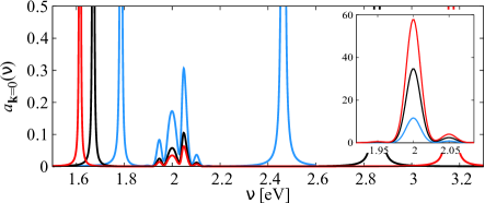
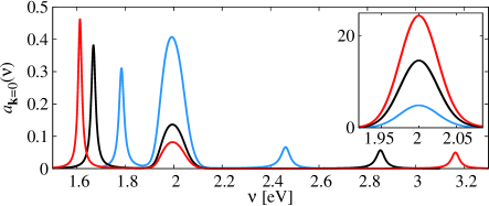
Figure 3: (color online) The evolution of absorption spectra with the strength of $g\sqrt{N}$ for a system with a single vibrational mode with $S=0.06,\Omega=0.05$eV. The insets show the equivalent absorption spectra for bare molecules. The other parameters are as in Fig. 1. Panel (a) shows the spectrum for a perfect cavity while panel (b) includes the effects of cavity losses and non-radiative excitonic decay exactly as in Fig. 1(b).

Figure 3 shows an equivalent set of spectra to Fig. 1, but with vibrational dressing. For comparison in the insets we show the absorption spectra of a bare molecule $\Im[\tilde{\Sigma}_{\mathbf{k},xx}(\nu)]$, i.e. the spectra without a cavity. Panel (a) shows the simple case where cavity losses are ignored, while panel (b) shows the more experimentally relevant case where these effects are included (discussed in appendix A). In the following we use the notation $p-q$ which denotes transitions in the molecule from the state with $p$ vibrational excitations in the electronic ground state to the state with $q$ vibrational excitations in the electronic excited state. The presence of the vibrational modes causes dramatic changes to the residual excitonic peak in the polariton spectrum not seen in the bare excitonic absorption. For the bare molecule the spectral weight associated with transition with the “zero phonon line”, i.e. the transition denoted $0-0$ in the notation introduced above is completely dominant, only a small amount of weight visible in the sideband which corresponds to $0-1$ transition. When the molecule is placed inside a cavity, the vibrational sidebands corresponding to the $1-0$ and $0-1$ transitions become much more prominent. Physically this is because the spectral weight that had been associated with the $0-0$ transition in the bare molecular spectrum has been moved into the polariton peaks of the spectrum. The mathematical form of the Green’s function makes clear that formation of the polariton spectral feature is predominantly at the expense of whatever feature dominates the excitonic emission spectrum; here this is the $0-0$ feature. The excitonic feature corresponds to the “left-over” spectral weight associated with the subradiant states. Thus, the vibrational sidebands have been “excavated” by removing the dominant feature from the zero-phonon line. Including the the effects of cavity losses and non-radiative excitonic decays, as can be seen in Fig. 3 (b), washes out this complex sideband structure of the central peaks and the spectrum as a function of coupling strength looks very similar to that obtained without coupling to vibrational modes, as in Fig. 1. However as we discuss below, there are still effects which can be observed which are a direct consequence of the vibrational structure.

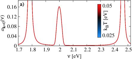
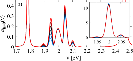
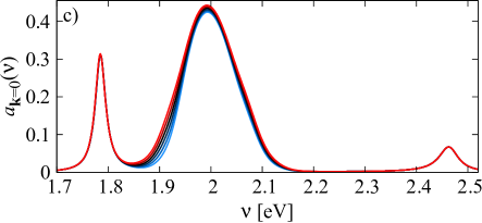
Figure 4: (color online) Evolution of absorption spectra with the temperature (values shown on the colorscale) for: (a) A system with no coupling to vibrational modes, $S=0$, (b) Coupling to a single vibrational mode with $S=0.02,\Omega=0.05$eV. The inset shows the bare molecular spectrum. (c) Including the effects of cavity losses and non-radiative excitonic decay. All panels are for $g\sqrt{N}=0.3$eV, and other parameters as in previous figures.

Fig. 4 illustrates the evolution of spectra with temperature. Panel (a) shows that without coupling to vibrational modes there is no notable temperature dependence. In the presence of the vibrational dressing, a strong temperature dependence appears. At higher temperatures, there is a greater thermal occupation of the vibrational modes hence the spectral weight under the vibrational peaks rises. While this has a small effect in the bare molecular spectrum (where the $0-0$ transition dwarfs all other features), see inset in (b), it is very pronounced in the polariton spectrum and is even visible in the presence of large cavity losses as in Fig. 4(c).

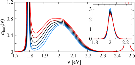
Figure 5: (color online) Temperature dependence of absorption spectrum for a system with strong disorder $\sigma=0.025eV$. The main panel shows the optical spectrum of the strongly coupled system, the inset shows the spectrum of the bare excitons. In this case, we include two vibrational modes: $S_{1}=0.2,\Omega_{1}=0.05$eV, and $S_{2}=0.3,\Omega_{2}=0.0$4eV. Other parameters as in Fig. 4.

The figures so far have shown results where disorder is relatively small, and so vibronic replicas can be clearly observed for the good cavity, but merge for the bad cavity limit. To show that small disorder is not required for the strong temperature dependence to occur Fig. 5 shows the effects of large disorder (i.e. inhomogeneous broadening). Just as seen for the homogeneous broadening in Fig. 4(c), a temperature dependence of the residual excitonic peak is still visible. In this figure, we have also included a more complicated vibrational spectrum, involving two vibrational modes. Such a system will exhibit behavior similar to that of a single mode but with a large vibrational coupling .

IV Discussion

In this paper we have presented two microscopic models which could in principle describe self-consistent molecular adaptation so as to maximize the vacuum-state coupling to light. In both cases, the crucial feature of the model is the counter-rotating terms in the matter-light coupling. These allow virtual fluctuations in the ground state, that lower the ground state energy depending on the configuration of the molecules. This energy gain is the only energy gain that can be relevant in the linear response regime — i.e. the question of whether the excited states would have lower energy is not of relevance while the system is only weakly pumped. We found that while such a mechanism for molecular adaptation does exist, it does not show any collective enhancement, in contrast to the polariton splitting, and does not therefore lead to significant molecular adaptation, even when the polariton splitting $g_{\mathbf{k}}\sqrt{N_{m}}\sim\omega,\epsilon$.

The appearance of a residual exciton peak in the polariton spectrum would be affected by any such self-consistent molecular adaptation if its scale were sufficient. However, for relevant parameters, such effects are dwarfed by a far more dramatic effect, of vibrational dressing of the residual exciton peak. This leads to a pronounced temperature dependence of the feature near the exciton energy in the absorption spectrum.

While the molecular adaptation energy scale is not collectively enhanced, the basic underlying physics could potentially be relevant in single molecule strong coupling, e.g. with plasmonic resonances Törmä and Barnes (2015). In such cases, rather than having many molecules in a large mode volume, the mode volume is reduced so that strong, or even ultra-strong coupling occurs at the single molecule level, so that both the polariton energy and the molecular adaptation energy become large. In such a case, one may hope to see either reorientation, or renormalization of the Huang-Rhys parameter due to strong coupling.

Another intriguing direction for future research is to consider how the physics discussed in this manuscript interacts with the physics of polariton condensation and lasing Carusotto and Ciuti (2013). Polariton condensation has been seen in both inorganic Kasprzak et al. (2006); Balili et al. (2007) and organic Kéna-Cohen et al. (2008); Kéna-Cohen and Forrest (2010); Plumhof et al. (2014); Daskalakis et al. (2014) systems. In addition, condensation of photons has been seen for weakly coupled systems of organic molecules Klaers et al. (2010). Theoretical work Litinskaya et al. (2004); Litinskaya and Reineker (2006); Litinskaya (2008); Michetti and La Rocca (2009); Fontanesi and La Rocca (2009); Mazza and La Rocca (2009); Mazza et al. (2013); Ćwik et al. (2014); Michetti et al. (2015) has begun to address some of the peculiarities of the organic polariton system, including effects of disorder and of vibrational modes. However, features as seen in this paper, resulting from the interplay of these may lead to further exotic behavior in the high density condensed phase.

Note added:

During the final preparation of this manuscript, another paper Galego et al. (2015) appeared, also reporting the fact that ground-state bond length depends on the single-molecule coupling $g$, not the collective coupling $g\sqrt{N_{m}}$.

Appendix A Absorption, Transmission and Reflection spectrum of exciton-polariton system

In this appendix we summarize the calculation of the absorption, transmission and reflection spectra. Some subtleties arise because we wish to calculate the spectrum of a model with ultrastrong coupling, i.e. without making the rotating wave approximation. Such results were first calculated by Ciuti and Carusotto (2006), here we present a synopsis of these results, as well as a “dictionary” to translate the results of that paper into the language of Green’s functions. We begin by defining the retarded Green’s function Abrikosov et al. (1975). Because we consider both co- and counter-rotating terms, we must consider both normal and anomalous Green’s functions. i.e. we must include number non-conserving terms which appear for ultrastrong coupling, and thus we consider a matrix Green’s function:

$$G^{R}_{\mathbf{k}}(t,t^{\prime})=-i\begin{pmatrix}\langle[\psi_{\mathbf{k}}(t),\psi^{\dagger}_{\mathbf{k}}(t^{\prime})]\rangle&\langle[\psi^{\dagger}_{-\mathbf{k}}(t),\psi^{\dagger}_{\mathbf{k}}(t^{\prime})]\rangle\\ \langle[\psi_{\mathbf{k}}(t),\psi_{-\mathbf{k}}(t^{\prime})]\rangle&\langle[\psi^{\dagger}_{-\mathbf{k}}(t),\psi_{-\mathbf{k}}(t^{\prime})]\rangle\end{pmatrix}$$

In terms of the Bogoliubov transformed operators, i.e. the operators appearing in Eq. (2) the inverse Green’s function takes the form

$$[\tilde{G}^{R}_{\mathbf{k}}(\nu)]^{-1}=\begin{pmatrix}\nu+i\tilde{\kappa}(\nu)-\tilde{\omega}_{\mathbf{k}}+\tilde{\Sigma}_{\mathbf{k},xx}(\nu)&+i\tilde{\kappa}(\nu)+\tilde{\Sigma}_{\mathbf{k},xx}(\nu)\\ -i\tilde{\kappa}^{\ast}(-\nu)+\tilde{\Sigma}^{\ast}_{\mathbf{k},xx}(-\nu)&-\nu-i\tilde{\kappa}^{\ast}(-\nu)-\tilde{\omega}_{\mathbf{k}}+\tilde{\Sigma}^{\ast}_{\mathbf{k},xx}(-\nu)\end{pmatrix},$$

where $\tilde{\Sigma}_{\mathbf{k},xx}(\nu)$ is the self energy for a photon of in-plane momentum $\mathbf{k}$, arising from the excitonic response (discussed further below), and $\tilde{\kappa}(\nu)$ is the loss rate. Here, following Ciuti and Carusotto (2006) we have used a frequency dependent complex loss rate $\tilde{\kappa}(\nu)$. Frequency dependence is required for physical consistency in the case of ultrastrong coupling — Markovian loss and ultrastrong coupling would predict a perpetual light source. Frequency dependent loss requires, via the Kramers-Kronig relation, a corresponding Lamb shift, which is incorporated into the imaginary part of $\tilde{\kappa}(\nu)$. Both $\tilde{\Sigma}$ and $\tilde{\kappa}$ are written for the Bogoliubov transformed operators, and so both these terms incorporate a pre-factor $\omega_{\mathbf{k}}/\tilde{\omega}_{\mathbf{k}}$ to account for the Bogoliubov transformation of the combination $(\hat{\psi}_{\mathbf{k}}+\hat{\psi}^{\dagger}_{-\mathbf{k}})$.

The specific self energy required, $\tilde{\Sigma}_{\mathbf{k},xx}(\nu)$, corresponds to correlation functions of the $\hat{\sigma}^{x}$ excitonic operators. In the absence of strong (i.e. beyond RWA) excitonic damping (see Ciuti and Carusotto (2006) for the more general case), this self energy can however be related to results in the rotating wave approximation by:

$$\tilde{\Sigma}_{\mathbf{k},xx}(\nu)=\frac{\omega_{k}}{\tilde{\omega}_{k}}\left(\Sigma^{\text{RWA}}_{\mathbf{k},+-}(\nu)+\left[\Sigma^{\text{RWA}}_{\mathbf{k},+-}(-\nu)\right]^{\star}\right),$$ (24)

where the expression $\Sigma^{\text{RWA}}_{\mathbf{k},+-}$ is the “standard” self energy that would appear in the rotating wave approximation, depending on the correlation of ${\hat{\sigma}}^{+},{\hat{\sigma}}^{-}$ operators. These can most easily be found by analytic continuation from imaginary time to real time, starting from the Matsubara self energy,

$$\Sigma^{\text{RWA}}_{\mathbf{k},+-}(i\omega_{m})=\frac{1}{\mathcal{Z}}\sum_{n}g_{\mathbf{k},n}^{2}\int_{0}^{\beta}\!\!d\tau e^{-i\omega_{m}\tau}\\ \times\sum_{p}\langle p|\hat{\sigma}_{n}^{+}(\tau)\hat{\sigma}_{n}^{-}(0)|p\rangle e^{-\beta E_{p}}$$ (25)

and replacing the Matsubara frequency by $i\omega_{m}\to\nu+i0^{+}$. The sum over $p$ appearing here is over all states of the excitonic system, and $\mathcal{Z}$ is the partition function. For the “vacuum” state we consider — i.e. in the absence of strong pumping — these are the bare exciton states, including the quantum states of any auxiliary degrees of freedom.

Using the input-output formalism Collett and Gardiner (1984) adapted to the ultrastrong coupling regime Ciuti and Carusotto (2006), one can write a frequency dependent scattering matrix relating input and output fields at the left and right sides of the cavity,

$$\mathcal{S}_{\mathbf{k}}(\nu)=\begin{pmatrix}1-i\phi_{\mathbf{k},L}(\nu)&-i\sqrt{\phi_{\mathbf{k},L}(\nu)\phi_{\mathbf{k},R}(\nu)}\\ -i\sqrt{\phi_{\mathbf{k},L}(\nu)\phi_{\mathbf{k},R}(\nu)}&1-i\phi_{\mathbf{k},R}(\nu)\end{pmatrix}$$

where $\phi_{\mathbf{k},\sigma}(\nu)=\kappa_{\sigma}^{\prime}(\nu)G^{R}_{\mathbf{k},xx}(\nu)$ with $\kappa_{L,R}^{\prime}(\nu)$ are the real parts of the loss rates arising from the left and right mirrors and the quantity $G^{R}_{\mathbf{k},xx}(\nu)$ relates to the matrix retarded Green’s function as $G^{R}_{\mathbf{k},xx}(\nu)=I^{T}G^{R}_{\mathbf{k}}(\nu)I$ where $I^{T}=\begin{pmatrix}1&1\end{pmatrix}$. This structure means the Bogoliubov transformation corresponds to $G^{R}_{\mathbf{k},xx}(\nu)=(\omega_{\mathbf{k}}/\tilde{\omega_{\mathbf{k}}})\tilde{G}^{R}_{\mathbf{k},xx}(\nu)$ and the Bogoliubov transformed Green’s function takes the form:

$$\tilde{G}^{R}_{\mathbf{k},xx}(\nu)=\frac{2\tilde{\omega}_{\mathbf{k}}}{\nu^{2}-\tilde{\omega}_{\mathbf{k}}^{2}+2\tilde{\omega}_{\mathbf{k}}\tilde{\Sigma}_{\mathbf{k},xx}(\nu)+i\tilde{\omega}_{\mathbf{k}}\tilde{\kappa}(\nu)}.$$ (26)

One can then find the transmission $T_{\mathbf{k}}(\nu)$, reflection $R_{\mathbf{k}}(\nu)$ and absorption $A_{\mathbf{k}}(\nu)$ coefficients by considering the modulus square of various coefficients. Clearly $T_{\mathbf{k}}(\nu)=\kappa_{L}^{\prime}(\nu)\kappa_{R}^{\prime}(\nu)|G^{R}_{\mathbf{k},xx}(\nu)|^{2}$ is independent of which direction light is incident from, while the absorption coefficient $A_{\mathbf{k},\sigma=L,R}(\nu)$ takes the form

$$A_{\mathbf{k},\sigma}(\nu)=-\kappa^{\prime}_{\sigma}(\nu)\left[2\Im\left[G^{R}_{\mathbf{k},xx}(\nu)\right]+\kappa(\nu)\left|G^{R}_{\mathbf{k},xx}(\nu)\right|^{2}\right],$$ (27)

with $\kappa(\nu)=(\kappa_{L}(\nu)+\kappa_{R}(\nu))/2$. The prefactor in this expression shows the obvious dependence on the transmissivity of the input mirrors.

In order to separate mirror transmissivity dependent features from the “intrinsic” properties of the ultrastrong coupling we will consider below the two quantities $t_{\mathbf{k}}(\nu)=|G^{R}_{\mathbf{k},xx}(\nu)|^{2}$ as being proportional to the transmission, and $a_{\mathbf{k}}(\nu)=-2\Im[G^{R}_{\mathbf{k},xx}(\nu)]$ as controlling the absorption in the limit of a good cavity, i.e. $\kappa(\nu)\to 0$. The quantity $a_{\mathbf{k}}(\nu)$ differs from the full absorption as it neglects interference effects at the input mirror.

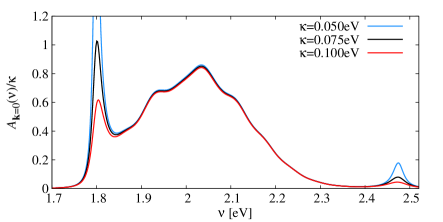
Figure 6: (color online) Absorption spectrum, as defined by the full expression, Eq. (27), plotted for $S_{1}=0.25$, $S_{2}=0.35$, $\Omega_{1}=0.06$eV, $\Omega_{2}=0.05$eV, $k_{B}T=0.035$eV and various cavity loss rates, $\kappa$. Other parameters are as in Fig. 5. As discussed in the text, in order that the polaritonic peaks have a finite width, one must include the effects of excitonic absorption or non-mirror cavity losses. For this figure, we include an excitonic linewidth $\gamma=10^{-4}$eV.

For comparison to the results in Ref. Canaguier-Durand et al. (2013) where silver mirrors were used, we present in Figures 1, 3, and 4 the effects of large cavity linewidth. Figure 6 also shows how the full absorption spectrum given by Eq. (27) evolves with varying linewidth. In calculating these spectra for large linewidth, an issue arises regarding the form of the absorption spectrum: The equations written above assume that the only photon loss is due to escape through the mirrors. This means that the $\kappa(\nu)$ appearing explicitly in Eq. (27) (describing interference effects from the mirror) is the same as the $\kappa(\nu)$ appearing in the denominator of the photon Green’s function, Eq. (26), and one may check that for any frequency where $\Im[\Sigma_{\mathbf{k},xx}(\nu)]$ is small, this causes a near cancellation between the two contributions. For the Gaussian exciton density of states $h(\epsilon)$ used in this paper, this cancellation almost completely suppresses the polariton peaks. Such a cancellation in the absorption spectrum can be expected on physical grounds: if the only loss channel for photons is the mirrors, then there is no absorption. All photons that enter eventually leave. In a real device there are other photon loss sources (absorbers, scattering by surface roughness). Similarly, in a real device, the excitons have a non-zero rate of non-radiative decay. The effect of this is included by retaining a non-zero value of $\gamma$ in the denominator of the self-energy, Eq. (23). This leads to Lorentzian tails of $\Im[\Sigma_{\mathbf{k},xx}(\nu)]$, giving a finite weight to the polariton peak in the absorption spectrum; such an effect was included by Houdré et al. (1996). We follow this approach in plotting Fig. 6.

Appendix B Schrieffer-Wolff transformation

In section II we make use of the Schrieffer-Wolff approximation; for completeness we provide here a brief explanation of this formalism. The approach is based on dividing the Hamiltonian into two parts, $\hat{H}=\hat{H}_{0}+\hat{H}_{1}$, where the term $\hat{H}_{1}$ takes one between different “sectors”. In our case, these sectors correspond to different numbers of polaritons — i.e. $H_{1}$ is the “counter-rotating” part of the Hamiltonian which simultaneous creates a photon and excites a molecule.

The aim of the Schrieffer-Wolff formulation is to make a unitary transformation $\hat{\tilde{H}}=e^{i\hat{G}}\hat{H}e^{-i\hat{G}}$ such that the transformed Hamiltonian no longer has any coupling between sectors. Physically, this corresponds to eliminating the effect of virtual pair creation and destruction, and deriving how such virtual processes renormalize the Hamiltonian within a given sector.

If the Hamiltonian $\hat{H}_{1}$ can be treated perturbatively by replacing $\hat{H}_{1}\to\eta\hat{H}_{1}$ with $\eta$ a small parameter, then one can consider a series solution $\hat{G}=\sum_{n=1}^{\infty}\eta^{n}\hat{G}_{(n)}$. In order to make the first-order terms in $\eta$ vanish, one must choose $[\hat{G}_{(1)},\hat{H}_{0}]=i\hat{H}_{1}$. This then leads (setting $\eta=1$) to the expression:

$$\tilde{\hat{H}}=\hat{H}_{0}+\frac{i}{2}\left[\hat{G}_{(1)},\hat{H}_{1}\right]+\text{H.o.t}$$ (28)

where the higher order terms involve all $\hat{G}_{(n>1)}$. Stopping at leading order gives the expression in Eq. (9), corresponding to the leading order effects of virtual pair creation and annihilation. To solve $[\hat{G}_{,}\hat{H}_{0}]=i\hat{H}_{1}$ in practice is straightforward if one knows the eigenspectrum of $H_{0}=\sum_{n}E^{(0)}_{n}|n\rangle\langle n|$, which then allows one to write

$$\hat{G}=i\sum_{n,m}\frac{|n\rangle\langle n|\hat{H}_{1}|m\rangle\langle m|}{E^{(0)}_{m}-E^{(0)}_{n}}.$$

References

- Hopfield (1958) J. Hopfield, Phys. Rev. 112, 1555 (1958).
- Pekar (1958) S. Pekar, Sov. J. Exp. Theor. Phys. 6, 785 (1958).
- Purcell (1946) E. M. Purcell, Phys. Rev. 69, 681 (1946).
- Björk et al. (1991) G. Björk, S. Machida, Y. Yamamoto, and K. Igeta, Phys. Rev. A 44, 669 (1991).
- Weisbuch et al. (1992) C. Weisbuch, M. Nishioka, A. Ishikawa, and Y. Arakawa, Phys. Rev. Lett. 69, 3314 (1992).
- Agranovich (1968) V. M. Agranovich, The Theory of Excitons (Nauka, Moscow, 1968).
- Davydov (1971) A. S. Davydov, Theory of Molecular Excitons (Plenum Press, New York, 1971).
- Agranovich (2009) V. M. Agranovich, Excitations in Organic Solids (Oxford University Press, Oxford, 2009).
- Lidzey et al. (1998) D. G. Lidzey, D. D. C. Bradley, M. S. Skolnick, T. Virgli, S. Walker, D. M. Whittaker, and T. Virgili, Nature 395, 53 (1998).
- Lidzey et al. (1999) D. G. Lidzey, D. D. C. Bradley, T. Virgili, A. Armitage, M. S. Skolnick, and S. Walker, Phys. Rev. Lett. 82, 3316 (1999).
- Schwartz et al. (2011) T. Schwartz, J. A. Hutchison, C. Genet, and T. W. Ebbesen, Phys. Rev. Lett. 106, 196405 (2011).
- Tischler et al. (2005) J. R. Tischler, M. S. Bradley, V. Bulović, J. H. Song, and A. Nurmikko, Phys. Rev. Lett. 95, 036401 (2005).
- Dicke (1954) R. Dicke, Phys. Rev. 93, 99 (1954).
- Michetti et al. (2015) P. Michetti, L. Mazza, and G. C. L. Rocca, Organic Nanophotonics, edited by Y. S. Zhao, Nano-Optics and Nanophotonics (Springer Berlin Heidelberg, Berlin, Heidelberg, 2015).
- Kéna-Cohen et al. (2008) S. Kéna-Cohen, M. Davanço, and S. R. Forrest, Phys. Rev. Lett. 101, 116401 (2008).
- Kéna-Cohen and Forrest (2010) S. Kéna-Cohen and S. R. Forrest, Nat. Photon. 4, 371 (2010).
- Plumhof et al. (2014) J. D. Plumhof, T. Stöferle, L. Mai, U. Scherf, and R. F. Mahrt, Nat. Mater. 13, 247 (2014).
- Daskalakis et al. (2014) K. S. Daskalakis, S. A. Maier, R. Murray, and S. Kéna-Cohen, Nat. Mater. 13, 271 (2014).
- Hutchison et al. (2012) J. A. Hutchison, T. Schwartz, C. Genet, E. Devaux, and T. W. Ebbesen, Angewandte Chemie 124, 1624 (2012).
- Orgiu et al. (2015) E. Orgiu, J. George, J. A. Hutchison, E. Devaux, J. F. Dayen, B. Doudin, F. Stellacci, C. Genet, P. Samori, and T. W. Ebbesen, Nat. Mat. 14, 1123 (2015).
- Schachenmayer et al. (2014) J. Schachenmayer, C. Genes, E. Tignone, and G. Pupillo, Phys. Rev. Lett. 114, 196403 (2015).
- Feist and Garcia-Vidal (2015) J. Feist and F. J. Garcia-Vidal, Phys. Rev. Lett. 114, 196402 (2015).
- Shalabney et al. (2015) A. Shalabney, J. George, J. A. Hutchison, G. Pupillo, C. Genet, and T. W. Ebbesen, Nat. Comm. 6, 5981 (2015).
- Roelli et al. (2014) P. Roelli, C. Galland, N. Piro, and T. J. Kippenberg, Nat. Nano. advance online publication, (2015).
- Pino et al. (2015) J. Pino, J. Feist, and F. J. Garcia-vidal, New J. Phys. 17, 053040 (2015).
- Pino et al. (2015) J. Pino, J. Feist, and F. J. Garcia-vidal, “Signatures of Vibrational Strong Coupling in Raman Scattering,” (2015), arXiv:1511.02115v1 .
- Spano (2015) F. C. Spano, J. Chem. Phys. 142, 184707 (2015).
- Canaguier-Durand et al. (2013) A. Canaguier-Durand, E. Devaux, J. George, Y. Pang, J. A. Hutchison, T. Schwartz, C. Genet, N. Wilhelms, J.-M. Lehn, and T. W. Ebbesen, Angew. Chem. Int. Ed. Engl. 52, 10533 (2013).
- Schwartz et al. (2013) T. Schwartz, J. A. Hutchison, J. Léonard, C. Genet, S. Haacke, and T. W. Ebbesen, Chem. Phys. Chem 14, 125 (2013).
- Houdré et al. (1996) R. Houdré, R. P. Stanley, and M. Ilegems, Phys. Rev. A 53, 2711 (1996).
- Eastham and Littlewood (2001) P. R. Eastham and P. B. Littlewood, Phys. Rev. B 64, 235101 (2001).
- Keeling et al. (2005) J. Keeling, P. R. Eastham, M. H. Szymanska, and P. B. Littlewood, Phys. Rev. B 72, 115320 (2005).
- Ciuti et al. (2005) C. Ciuti, G. Bastard, and I. Carusotto, Phys. Rev. B 72, 115303 (2005).
- De Liberato (2015) S. De Liberato, Phys. Rev. B 92, 125433 (2015).
- Anappara et al. (2009) A. A. Anappara, S. De Liberato, A. Tredicucci, C. Ciuti, G. Biasiol, L. Sorba, and F. Beltram, Phys. Rev. B 79, 201303 (2009).
- Gambino et al. (2014) S. Gambino, M. Mazzeo, A. Genco, O. Di Stefano, S. Savasta, S. Patanè, D. Ballarini, F. Mangione, G. Lerario, D. Sanvitto, and G. Gigli, ACS Photonics 1, 1042 (2014).
- Gubbin et al. (2014) C. Gubbin, S. Maier, and S. Kena-Cohen, Appl. Phys. Lett. 104 (2014).
- Maissen et al. (2014) C. Maissen, G. Scalari, F. Valmorra, M. Beck, J. Faist, S. Cibella, R. Leoni, C. Reichl, C. Charpentier, and W. Wegscheider, Phys. Rev. B 90, 205309 (2014).
- Rzazewski et al. (1975) K. Rzazewski, K. Wódkiewicz, and W. Zakowicz, Phys. Rev. Lett. 35, 432 (1975).
- Ciuti and Carusotto (2006) C. Ciuti and I. Carusotto, Phys. Rev. A 74, 033811 (2006).
- Schrieffer and Wolff (1966) J. R. Schrieffer and P. A. Wolff, Phys. Rev. 149, 491 (1966).
- Note (1) Note however that the collective splitting can however still be comparable to , as is indeed the case for the parameters we consider.
- Casanova et al. (2010) J. Casanova, G. Romero, I. Lizuain, J. J. Garcia-Ripoll, and E. Solano, Phys. Rev. Lett. 105, 263603 (2010).
- De Liberato (2014) S. De Liberato, Phys. Rev. Lett. 112, 016401 (2014).
- Kim et al. (2015) M.-K. Kim, H. Sim, S. J. Yoon, S.-H. Gong, C. W. Ahn, Y.-H. Cho, and Y.-H. Lee, Nano Lett. 15, 4120 (2015).
- Caldwell et al. (2013) J. D. Caldwell, O. J. Glembockl, Y. Francescato, N. Sharac, V. Glannini, F. J. Bezares, J. P. Long, J. C. Owrutsky, I. Vurgaftman, J. G. Tischler, V. D. Wheeler, N. D. Bassim, L. M. Shirey, R. Kaslca, and S.-A. Maler, Nano Lett. 13, 3690 (2013).
- De Liberato et al. (2009) S. De Liberato, D. Gerace, I. Carusotto, and C. Ciuti, Phys. Rev. A 80, 053810 (2009).
- Note (2) One may note that if the vibrational modes were degenerate , then the effective Huang-Rhys parameter will be .
- Törmä and Barnes (2015) P. Törmä and W. L. Barnes, Reports on Progress in Physics 78, 013901 (2015).
- Carusotto and Ciuti (2013) I. Carusotto and C. Ciuti, Rev. Mod. Phys. 85, 299 (2013).
- Kasprzak et al. (2006) J. Kasprzak, M. Richard, S. Kundermann, A. Baas, P. Jeambrun, J. M. J. Keeling, F. M. Marchetti, M. H. Szymanska, R. André, J. L. Staehli, V. Savona, P. B. Littlewood, B. Deveaud, and L. S. Dang, Nature 443, 409 (2006).
- Balili et al. (2007) R. Balili, V. Hartwell, D. Snoke, L. Pfeiffer, and K. West, Science (80-. ). 316, 1007 (2007).
- Klaers et al. (2010) J. Klaers, J. Schmitt, F. Vewinger, and M. Weitz, Nature 468, 545 (2010).
- Litinskaya et al. (2004) M. Litinskaya, P. Reineker, and V. M. Agranovich, Phys. Stat. Sol. 201, 646 (2004).
- Litinskaya and Reineker (2006) M. Litinskaya and P. Reineker, Phys. Rev. B 74, 165320 (2006).
- Litinskaya (2008) M. Litinskaya, Phys. Rev. B 77, 155325 (2008).
- Michetti and La Rocca (2009) P. Michetti and G. C. La Rocca, Phys. Rev. B 79, 035325 (2009).
- Fontanesi and La Rocca (2009) L. Fontanesi, L. Mazza, and G. C. La Rocca, Phys. Rev. B 80, 235313 (2009).
- Mazza and La Rocca (2009) L. Mazza, L. Fontanesi and G. C. La Rocca, Phys. Rev. B 80, 235314 (2009).
- Mazza et al. (2013) L. Mazza, S. Kéna-Cohen, P. Michetti, and G. C. La Rocca, Phys. Rev. B 88, 075321 (2013).
- Ćwik et al. (2014) J. A. Ćwik, S. Reja, P. B. Littlewood, and J. Keeling, Eur. Lett. 105, 47009 (2014).
- Galego et al. (2015) J. Galego, F. J. Garcia-Vidal, and J. Feist, Phys. Rev. X 5, 041022 (2015).
- Abrikosov et al. (1975) A. Abrikosov, L. Gorkov, and I. Dzyaloshinski, Methods of Quantum Field Theory in Statistical Physics (Dover, New York, 1975).
- Collett and Gardiner (1984) M. J. Collett and C. W. Gardiner, Phys. Rev. A 30, 1386 (1984).