Anomalous Spin Response and Virtual-Carrier-Mediated Magnetism in a Topological Insulator

Abstract

We present a comprehensive theoretical study of the static spin response in HgTe quantum wells, revealing distinctive behavior for the topologically nontrivial inverted structure. Most strikingly, the ${\bm{\mathrm{q}}}=0$ (long-wave-length) spin susceptibility of the undoped topological-insulator system is constant and equal to the value found for the gapless Dirac-like structure, whereas the same quantity shows the typical decrease with increasing band gap in the normal-insulator regime. We discuss ramifications for the ordering of localized magnetic moments present in the quantum well, both in the insulating and electron-doped situations. The spin response of edge states is also considered, and we extract effective Landé $g$-factors for the bulk and edge electrons. The variety of counter-intuitive spin-response properties revealed in our study arises from the system’s versatility in accessing situations where the charge-carrier dynamics can be governed by ordinary Schrödinger-type physics, mimics the behavior of chiral Dirac fermions, or reflects the material’s symmetry-protected topological order.

I Introduction & Main Results

The two-dimensional (2D) topological insulator (TI) realized in inverted HgTe quantum wells exhibits unusual electric-transport properties König et al. (2007); Roth et al. (2009); Brüne et al. (2012); Hart et al. that have attracted great interest Qi and Zhang (2011). TI behavior is also found in other 2D Liu et al. (2008a); Knez et al. (2011) and bulk Qi and Zhang (2011); Hasan and Moore (2011) materials. The potential for interesting interplays between a TI’s electronic and magnetic degrees of freedom, e.g., through hyperfine interaction with the material’s nuclei Lunde and Platero (2013), or local exchange interaction with magnetic dopants Novik et al. (2005), has been pointed out recently Liu et al. (2008b); Yu et al. (2010). These efforts have opened up new perspectives and extended previous work devoted to understanding spin effects Simon and Loss (2007); Simon et al. (2008) and magnetism Dietl (2010) in ordinary semiconductors. Our present theoretical study of the spin response in HgTe quantum wells reveals unconventional spin-related properties that distinguish this paradigmatic TI material from all other currently known 2D electronic systems. We thus provide alternative means for the experimental identification of the topological regime and extend current knowledge about the fundamentals of spin-response behavior in solids.

The spin susceptibility contains comprehensive information about the magnetic properties of a material. In the simplest case of a spin-rotationally invariant noninteracting electron gas, the spin susceptibility is proportional to the charge-response (Lindhard) function Giuliani and Vignale (2005). Noticable deviations from that situation occur, e.g., in systems with strong spin-orbit coupling such as 2D hole gases Kernreiter et al. (2013). For metals or degenerately doped semiconductors, the spin response of only the partially filled band is typically considered. This approach misses intrinsic contributions to many-particle response functions arising from virtual interband transitions that become important in narrow-gap and, especially gapless, electron systems. Examples for the latter are the 2D Dirac-like electron states on the surface of a bulk TI whose magnetic properties have been discussed in Refs. Liu et al., 2009; Zhu et al., 2011. The HgTe quantum wells considered here present an ideal testing ground for exploring the importance and properties of intrinsic, or virtual-carrier, effects, as it is possible to tune the band gap in such systems with a single structural parameter (i.e., the quantum-well width $d$). Furthermore, deviations from the conical 2D-Dirac dispersion in the gapless case are well characterized within a continuum-model (BHZ) description Bernevig et al. (2006) that also gives controlled access to the full range of, and interesting transitions between, Schrödinger-physics-dominated, chiral-Dirac-fermion-like, and topologically nontrivial phases. In particular, definite (i.e., cut-off-independent) results for the intrinsic response at long wavelengths are obtained even in the limit of vanishing band gap; unlike in the case of the previously considered 2D-Dirac models used to describe the surface states of bulk TIs Liu et al. (2009); Zhu et al. (2011).

Before going into greater detail in the remainder of this Article, we briefly highlight four major advances and central new insights gained from our work.

(i) We find an analytical expression for the uniform static spin susceptibility of the intrinsic (undoped) system,

$$\overline{\chi}^{(\text{int})}_{xx,zz}(\gamma;{\bm{\mathrm{q}}}=0)=-\frac{\mathcal{C}^{2}_{x,z}(\gamma)}{16\pi|B|}\,\frac{1}{1+4\xi_{\text{M}}\Theta(\xi_{\text{M}})}\quad,$$ (1)

where $\xi_{\text{M}}$ is proportional to the band gap and positive (negative) for the topologically trivial normal (topologically nontrivial inverted) regime, $\Theta$ denotes the Heaviside step function, $B$ is a band-structure parameter from the BHZ model introduced further below, and the constants $\mathcal{C}_{x,z}(\gamma)$ depend both on the valence-band mixing of quantum-well basis states and on the parameter $\gamma$ that characterises the relative coupling strength of the conduction-band and valence-band spin degree of freedom to the physical quantity of interest. While the intrinsic spin response is suppressed with increasing band gap in the normal regime ($\xi_{M}>0$), it becomes independent of gap size in the topological regime where $\xi_{M}\leq 0$. This unexpected behavior is a special feature of the symmetry-protected topological phase of the bulk system associated with the existence of gapless edge states.

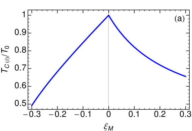
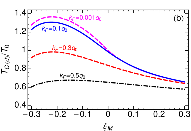
Figure 1: (a) Mean-field critical temperature $T_{\mathrm{C(i)}}$ for virtual-carrier-mediated magnetism in a HgTe quantum well plotted as a function of the band-gap parameter $\xi_{\text{M}}$. Note the striking asymmetry between the topological ($\xi_{M}<0$) and normal ($\xi_{M}>0$) regimes. An explicit expression for $T_{0}$ is given in the text; it contains the local exchange coupling between magnetic-impurity orbitals and HgTe quantum-well basis states, which is roughly constant across the transition Kossut and Dobrowolski (1997). (b) Critical temperature $T_{\mathrm{C(d)}}$ for the electron-doped HgTe quantum well plotted as a function of $\xi_{\text{M}}$ and for various charge-carrier densities (corresponding to indicated values for the Fermi wave vector $k_{\mathrm{F}}$; where $k_{\mathrm{F}}=q_{0}$ corresponds to a charge density $n_{0}\equiv q_{0}^{2}/(2\pi)=4.25\times 10^{12}\,$cm^-2 for a typical structure Rothe et al. (2010)). We used $\xi_{\text{D}}=-0.7$ for the BHZ-model electron-hole-asymmetry parameter in both plots, and $\gamma=-2.22$ as relevant for the (Hg,Cd,Mn)Te system Kossut and Dobrowolski (1997).

(ii) A physical consequence of the unusual spin response in the intrinsic system is the asymmetric variation of the critical (Curie) temperature for virtual-carrier-mediated magnetic order in a HgTe quantum well that has been doped magnetically but not electronically. See Fig. 1(a). A similarly striking asymmetry arises when charge carriers are present in the 2D conduction band; which is illustrated in Fig. 1(b). Furthermore, in this situation, a rather strong, and counter-intuitive, suppression of the Curie temperature with the density of itinerant charge carriers is revealed. This tendency arises from the unconventional character of conduction-band states in the topological regime. See Section III.2 for details.

(iii) We extract the effective g factors for 2D conduction electrons in both the topological and normal regimes, which are directly accessible experimentally Hart et al. . Their strong density and gap-parameter dependences reflect the band mixing and transition between regimes dominated by Schrödinger-type and Dirac-like dynamics of charge carriers. Full details can be found in Section IV. These results are essential, e.g., to enable quantitative characterization of the transition between quantum spin-Hall and quantum anomalous Hall phases in magnetic 2D topological insulators Liu et al. (2008b).

(iv) We predict the effective g factors of the helical edge states that are present in the topological regime of the HgTe quantum well. For the out-of-plane magnetic-field direction, the g factor assumes a constant value that is determined by band mixing in the quantum-well eigenstates. In contrast, the in-plane g factor has a strong density dependence. See Section V.

In the following, we discuss relevant details of our theoretical analysis and present complete results for the spin response in both intrinsic and electron-doped systems.

II Quantum-well bandstructure

The electronic properties of HgTe quantum wells are adequately captured by an effective four-band (BHZ) Hamiltonian Bernevig et al. (2006) that acts in the low-energy subspace spanned by basis states $|E_{1}+\rangle,|H_{1}+\rangle,|E_{1}-\rangle,|H_{1}-\rangle$ and explicitly reads

$$\mathscr{H}_{0}=\begin{pmatrix}{\mathcal{H}}({\bm{\mathrm{k}}})&0\\[5.69054pt] 0&{\mathcal{H}}^{*}(-{\bm{\mathrm{k}}})\end{pmatrix}~{},$$ (2)

with ${\mathcal{H}}({\bm{\mathrm{k}}})=h_{\mu}\sigma^{\mu}$, $h=(C-Dk^{2},Ak_{x},Ak_{y},M-Bk^{2})$ and $\sigma^{\mu}=(\openone,{\bm{\mathrm{\sigma}}})$. The parameters $A,B,C,D,M$ are functions of the well width $d$, and their numerical values are typically obtained by a fitting procedure Mühlbauer et al. (2014). The parameter $M$ opens a band gap, where (in the convention $B<0$) the system is in the topological (normal) regime when $M<0$ ($M>0$). The basis functions $|E_{1}\pm\rangle$ are a superposition of conduction-electron and light-hole (LH) basis functions with a given spin projection. The associated band $|L_{1}\pm\rangle$ has a much lower band-edge energy and can therefore be omitted. On the other hand, the heavy-hole (HH) states $|H_{1}\pm\rangle$ also belong to the set of low-energy excitations. In the following we set $C=0$, and employ a dimensionless description of Eq. (2) that is obtained by defining an energy scale $E_{0}\equiv Aq_{0}$ and a scale for the wave vector $q_{0}\equiv A/|B|~{}$Juergens et al. (2014a, b). (In a typical HgTe quantum-well structure Rothe et al. (2010), $E_{0}=0.189$ eV and $q_{0}=0.517$ nm^-1.) By making use of the axial symmetry of the BHZ Hamiltonian (2) we rotate to a real basis to obtain $\mathcal{H}^{\prime}({\bm{\mathrm{k}}})=U^{(+)\dagger}_{\phi_{\bm{\mathrm{k}}}}\mathcal{H}({\bm{\mathrm{k}}})U^{(+)}_{\phi_{\bm{\mathrm{k}}}}=E_{0}h^{\prime}_{\mu}\sigma^{\mu}$, with $U^{(s)}_{\phi_{\bm{\mathrm{k}}}}={\text{diag}}(\mathrm{e}^{is\phi_{\bm{\mathrm{k}}}/2},\mathrm{e}^{-is\phi_{\bm{\mathrm{k}}}/2})$ and $h^{\prime}=(-\xi_{\text{D}}\tilde{k}^{2},\tilde{k},0,\xi_{\text{M}}+\tilde{k}^{2})$, where $\phi_{\bm{\mathrm{k}}}$ is the polar angle of the 2D wave vector ${\bm{\mathrm{k}}}$. We have defined the dimensionless parameters $\xi_{\text{M}}\equiv M/E_{0}$ and $\xi_{\text{D}}\equiv D/|B|$, which have typical values Bernevig et al. (2006); Rothe et al. (2010); Mühlbauer et al. (2014) $|\xi_{\text{M}}|,|\xi_{\text{D}}|\lesssim 0.5$. The eigenvectors in the complex and real basis are related via $a^{(s)}_{{\bm{\mathrm{k}}}\alpha}=U^{(s)}_{\phi_{\bm{\mathrm{k}}}}~{}a^{(s)}_{k\alpha}$, where $\alpha=\pm$ distinguishes the conduction and valence bands, which are doubly degenerate in the quantum number $s=\pm$ for spin projection along the growth direction and have the dispersions

$$E_{{\bm{\mathrm{k}}}\alpha}^{(s)}\equiv E_{k\alpha}^{(s)}=E_{0}[-\tilde{k}^{2}\xi_{\text{D}}+\alpha\sqrt{(\xi_{\text{M}}+\tilde{k}^{2})^{2}+\tilde{k}^{2}}]\,\,.$$ (3)

III Effective spin susceptibility of the 2D system: Intrinsic & doped cases

The spin susceptibility is used to characterize a system’s response to spin-related external stimuli within the framework of linear-response theory Giuliani and Vignale (2005). In the static limit, and for quantum-well-confined electrons, it can be written as Kernreiter et al. (2013)

$$\chi_{ij}({\bm{\mathrm{R}}},z;{\bm{\mathrm{R}}}^{\prime},z^{\prime})=\lim_{\eta\to 0^{+}}\bigg{\{}-\frac{i}{\hbar}\int_{0}^{\infty}dt\,\,\mathrm{e}^{-\eta t}$$

$$\hskip 85.35826pt\times\langle[S_{i}({\bm{\mathrm{R}}},z;t)\,,\,S_{j}({\bm{\mathrm{R}}}^{\prime},z^{\prime};0)]\rangle\,\bigg{\}}\,,\quad$$ (4)

with ${\bm{\mathrm{R}}}\equiv(x,y)$ and $z$ being coordinates in the 2D plane and perpendicular to it, respectively, and $S_{j}({\bm{\mathrm{R}}},z)=\Psi^{\dagger}({\bm{\mathrm{R}}},z)~{}\hat{S}_{j}~{}\Psi({\bm{\mathrm{R}}},z)$ denoting the electron spin density measured in units of $\hbar$. For a homogeneous 2D electron system, the spin susceptibility is most straightforwardly obtained in terms of the spatially Fourier-transformed quantity $\chi_{ij}({\bm{\mathrm{q}}};z,z^{\prime})$ via

$$\chi_{ij}({\bm{\mathrm{R}}},z;{\bm{\mathrm{R}}}^{\prime},z^{\prime})=\int\frac{d^{2}q}{(2\pi)^{2}}\,\,\mathrm{e}^{i{\bm{\mathrm{q}}}\cdot({\bm{\mathrm{R}}}-{\bm{\mathrm{R}}}^{\prime})}\,\,\chi_{ij}({\bm{\mathrm{q}}};z,z^{\prime})\,.$$ (5)

The dependence of $\chi_{ij}({\bm{\mathrm{q}}};z,z^{\prime})$ on the coordinates $z$ and $z^{\prime}$ encodes the spatial profile of the quantum-well bound states. Within the BHZ framework, the $z$-dependent part of electron wave functions is contained in the four basis functions $|E_{1}\pm\rangle,|H_{1}\pm\rangle$. The latter are spinors whose explicit form has been derived Bernevig et al. (2006) within the six-band Kane-model description Winkler (2003) for the charge-carrier dynamics that includes the bands with $\Gamma_{6}$ and $\Gamma_{8}$ symmetry closest to the bulk-material’s fundamental gap. As is generally the case in multi-band systems, the spin response of electrons in a HgTe quantum well is strongly influenced by both the in-plane dynamics described by the BHZ Hamiltonian and the nontrivial spinor structure of the BHZ-model basis states. We therefore need to express the spin susceptibility within the underlying six-band Kane model.

The coupling between some physical stimulus represented by a field ${\bm{\mathrm{\mathcal{F}}}}$ and the $\Gamma_{6}$ and $\Gamma_{8}$-band intrinsic angular-momentum degrees of freedom ${\bm{\mathrm{\hat{\sigma}}}}$ and ${\bm{\mathrm{\hat{J}}}}$ is most generally described by a term

$${\mathscr{H}}_{{\bm{\mathrm{\mathcal{F}}}}}=\sum_{i}{\mathcal{F}}_{i}\left(b_{\Gamma_{6}}\,\frac{\hat{\sigma}_{i}}{2}\oplus 0_{4\times 4}+b_{\Gamma_{8}}\,0_{2\times 2}\oplus\hat{J}_{i}\right)$$ (6)

in the Kane-model Hamiltonian. See, e.g., Table C.5 in Ref. Winkler, 2003. Within this approach, the coefficients $b_{\Gamma_{j}}$ are intra-band coupling constants with appropriately renormalized values to take account of all field-induced band-coupling effects in the bulk material. To be able to discuss a wide range of spin-related phenomena, we define an effective (pseudo-)spin operator

$$\hat{S}_{i}(\gamma)=\frac{\hat{\sigma}_{i}}{2}\oplus(\gamma\hat{J}_{i})\quad,$$ (7)

such that ${\mathscr{H}}_{{\bm{\mathrm{\mathcal{F}}}}}\equiv b_{\Gamma_{6}}\sum_{i}{\mathcal{F}}_{i}\,\hat{S}_{i}(b_{\Gamma_{8}}/b_{\Gamma_{6}})$. The actual value of the parameter $\gamma$ depends on the physical quantity or situation of interest . The system’s response is then fully captured by the effective spin-susceptibility tensor

$$\chi_{ij}(\gamma;{\bm{\mathrm{q}}};z,z^{\prime})=\sum_{\alpha,\beta,s,s^{\prime}}\int\frac{d^{2}k}{(2\pi)^{2}}\,\,\mathscr{W}_{ij({\bm{\mathrm{k}}},{\bm{\mathrm{k}}}+{\bm{\mathrm{q}}},\alpha,\beta)}^{(s,s^{\prime})}(\gamma;z,z^{\prime})$$

$$\hskip 85.35826pt\times\frac{n_{\text{F}}(E^{(s)}_{{\bm{\mathrm{k}}}\alpha})-n_{\text{F}}(E^{(s^{\prime})}_{{\bm{\mathrm{k}}}+{\bm{\mathrm{q}}}\beta})}{E^{(s)}_{{\bm{\mathrm{k}}}\alpha}-E^{(s^{\prime})}_{{\bm{\mathrm{k}}}+{\bm{\mathrm{q}}}\beta}+i\hbar\eta}~{},$$ (8a)

where $$n_{\text{F}}$$ denotes the Fermi function, and

$$\mathscr{W}_{ij({\bm{\mathrm{k}}},{\bm{\mathrm{k}}}+{\bm{\mathrm{q}}},\alpha,\beta)}^{(s,s^{\prime})}(\gamma;z,z^{\prime})=\left[\psi^{(s)}_{{\bm{\mathrm{k}}}\alpha}(z)\right]^{\dagger}\cdot\Big{[}\hat{S}_{i}(\gamma)\,\psi^{(s^{\prime})}_{{\bm{\mathrm{k}}}+{\bm{\mathrm{q}}}\beta}(z)\Big{]}$$

$$\hskip 56.9055pt\times\Big{[}\psi^{(s^{\prime})}_{{\bm{\mathrm{k}}}+{\bm{\mathrm{q}}}\beta}(z^{\prime})\Big{]}^{\dagger}\cdot\Big{[}\hat{S}_{j}(\gamma)\,\psi^{(s)}_{{\bm{\mathrm{k}}}\alpha}(z^{\prime})\Big{]}~{},$$ (8b)

are matrix elements of the effective spin operator given in Eq. (7). In the spirit of subband ${\bm{\mathrm{k}}}\cdot{\bm{\mathrm{p}}}$ theory, the six-dimensional spinor wave functions $\psi^{(s)}_{{\bm{\mathrm{k}}}\alpha}(z)$ can be expressed in terms of the BHZ-model basis state spinors $\psi^{(s)}_{0i}(z)$ as

$$\psi^{(s)}_{{\bm{\mathrm{k}}}\alpha}(z)=\sum^{2}_{i=1}\left(U^{(s)}_{\phi_{\bm{\mathrm{k}}}}\right)_{ii}a_{k\alpha,i}^{(s)}~{}\psi_{0i}^{(s)}(z)~{},$$ (9)

where the coefficients $a_{k\alpha,i}^{(s)}$ are the components of the corresponding eigenvectors of the BHZ Hamiltonian (see Sec. II). The explicit form of the basis states was derived in Ref. Bernevig et al., 2006 by solving a confined-particle problem in the HgTe/CdTe hybrid system. For instance, $\psi^{(+)}_{01}(z)^{T}=(f_{1}(z),0,0,f_{4}(z),0,0)$, with the detailed form of the envelope function components $f_{i}(z)$ provided in the supplemental information of Ref. Bernevig et al., 2006.

In the following, we consider the growth-direction-averaged spin susceptibility of charge carriers in the HgTe quantum well, given by $\overline{\chi}_{ij}(\gamma;{\bm{\mathrm{q}}})=\int dz\int dz^{\prime}~{}\chi_{ij}(\gamma;{\bm{\mathrm{q}}};z,z^{\prime})$ Kernreiter et al. (2013), with $\chi_{ij}(\gamma;{\bm{\mathrm{q}}};z,z^{\prime})$ calculated using the Kane-model-based BHZ approach as described above. Note that, by replacing the spin matrices in Eq. (8) by the unit matrix and averaging over $z,z^{\prime}$, we obtain the charge-response function studied in Refs. Juergens et al., 2014a, b. From the axial symmetry of our Kane-model description, and the fact that the eigenstates have definite spin projection in the growth direction, it follows that the in-plane spin susceptibilities are the same, i.e., $\overline{\chi}_{xx}(\gamma;q)=\overline{\chi}_{yy}(\gamma;q)$, and only depend on the magnitude $q\equiv|{\bm{\mathrm{q}}}|$. This is an important difference to other semiconducting systems where HH-LH mixing occurs Kernreiter et al. (2013). In the present situation, HH-LH mixing arises only from terms linear in ${\bm{\mathrm{k}}}$ (giving rise to Dirac-like excitations) which is a consequence of the envelope function components Bernevig et al. (2006) behaving differently (even or odd) under the parity transformation $z\leftrightarrow-z$.

III.1 Spin response of the intrinsic system

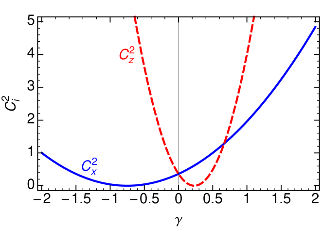
Figure 2: Prefactors $C_{x}^{2}$ and $C_{y}^{2}$ determining the magnitude of intrinsic in-plane and out-of-plane spin response, respectively [see Eq. (1)], plotted as a function of the parameter $\gamma$ from the definition of the effective Kane-model spin operator (7).

In the insulating limit, the conduction band is empty and the Fermi level lies in the band gap, i.e., $|\mu|<E_{0}|\xi_{\text{M}}|$. In this situation, the spin susceptibility originates from virtual interband transitions across the band gap. In the following we will focus on the zero temperature limit. The analytical result for the intrinsic spin susceptibility obtained in the limit of zero momentum transfer $q\to 0$ is given in Eq. (1), where

$${\mathcal{C}}_{x}(\gamma) = 1+(2\gamma-1)\,\mathcal{C}_{\text{LH}}\quad,$$ (10a)

$${\mathcal{C}}_{z}(\gamma) = 1-3\gamma+(\gamma-1)\,\mathcal{C}_{\text{LH}}\quad,$$ (10b)

and $\mathcal{C}_{\text{LH}}\equiv\int dz|f_{4}(z)|^{2}$ ($\approx 0.4$) is the amount of LH admixture in the basis states $|E_{1}\pm\rangle$. (Details about the calculation of the intrinsic spin susceptibility are given in Appendix A. Results for $q\neq 0$ can be calculated numerically. For completeness, some of these are also shown in Appendix A.) Equation (1) exhibits anomalous behavior in the inverted region ($\xi_{\text{M}}<0$) in that the uniform spin response is independent of the gap size and pinned to the value for the gapless case, even though it arises from virtual inter-band transitions. In the normal region ($\xi_{\text{M}}>0$), the expected decrease of the response functions with increasing band gap is found. The spin susceptibility (1) is strongly anisotropic, generally exhibiting a dominant out-of-plane response except for a very small range of the parameter $\gamma$. See Fig. 2.

A non-vanishing $\overline{\chi}^{(\text{int})}_{jj}(\gamma;0)$ seems to imply the counterintuitive phenomenon that an applied magnetic field could generate a magnetisation of the HgTe quantum-well system in the intrinsic limit where no charge carriers are present. Our more detailed analysis shows, however, that this is not the case. Direct calculation of the derivative of the free energy with respect to magnetic-field strength in a model based on the BHZ Hamiltonian (2) augmented by a Zeeman term reveals that the total magnetisation is strictly zero . This is due to the fact that intrinsic-spin and orbital contributions to the magnetization cancel, as expected in a spin-orbit-coupled system . This conclusion is further underpinned by the observation that $\overline{\chi}^{(\text{int})}_{jj}(\gamma;0)$ vanishes in the limit of zero HH-LH mixing .

As it is possible to engineer and study effective exchange interactions between impurity atoms Zhou et al. (2010); Khajetoorians et al. (2012), it is tempting to consider such interactions between two localized spins in a HgTe quantum well. Quite generally, the RKKY Hamiltonian is given by Yosida (1996)

$$\mathscr{H}^{\text{eff}}_{{\bm{\mathrm{r}}},{\bm{\mathrm{r}}}^{\prime}}=G^{2}\sum_{i,j}~{}I^{i}_{{\bm{\mathrm{r}}}}~{}I^{j}_{{\bm{\mathrm{r}}}^{\prime}}~{}\chi_{ij}({\bm{\mathrm{r}}},{\bm{\mathrm{r}}}^{\prime}).$$ (11)

Here $\chi_{ij}({\bm{\mathrm{r}}},{\bm{\mathrm{r}}}^{\prime})$, the Fourier transform of (8), is the spin susceptibility in real space, $I^{i}_{{\bm{\mathrm{r}}}}$ denotes the $i$th Cartesian component of an impurity spin located at position ${\bm{\mathrm{r}}}=({\bm{\mathrm{R}}},z)$, and $G$ is the local exchange-coupling constant between the spin degree of freedom carried by band electrons and localized (e.g., impurity) spins. (The difference in exchange-coupling strengths for conduction-band and valence-band states is accounted for by the appropriate value of $\gamma$.) In Fig. 3(a), we plot the growth-direction-averaged effective out-of-plane real-space spin susceptibility $\overline{\chi}_{zz}(R)$ as a function of the distance $R$ for various values of $\xi_{\text{M}}$ (and $\xi_{\text{D}}=-0.7$ corresponding to realistic situations Mühlbauer et al. (2014)).

Figure 3 shows that the effective exchange interaction mediated by the intrinsic spin response of the HgTe quantum well for localized spins is of ferromagnetic (FM) type if $Rq_{0}\ll 1$, and that there is a cross-over to antiferromagnetic (AFM) coupling for $Rq_{0}\gtrsim 1$ that sensitively depends on $\xi_{\text{M}}$. In particular, we find that this cross-over is shifted significantly to smaller impurity-spin separations in the case of the inverted regime as compared to the normal regime. Also, the magnitude of exchange interaction in the ferromagnetic regime for fixed distance $R$ markedly increases when enlarging the gap in the inverted system. In contrast, the exchange interactions in the normal regime have a very small magnitude. To further illustrate the parametric dependencies of the carrier-mediated exchange interaction, Fig. 3(b) shows the various regions of preferential spin alignments as a function of $\xi_{\text{M}}<0$. Interestingly, inbetween the two out-of-plane localized-spin alignments (FM_⟂ and AFM_⟂), we also find sizeable regions for the distance where it is energetically favorable for impurity spins to align ferromagnetically in-plane (FM_∥). Moreover, for larger distances, we find the usual Bloembergen-Rowland Bloembergen and Rowland (1955) behavior for the intrinsic spin susceptibilities which is characterized by an exponential decay factor that depends on the band gap, approximately given by $\sim\exp{(-R/R_{0})}/R^{3}$ where $R_{0}=(|\xi_{\text{M}}|q_{0})^{-1}$ is the Compton wave length of the band electrons. More details are given in Appendix B. In the limit of zero gap ($\xi_{\text{M}}\to 0$), the $R^{-3}$ decay found previously in various Dirac systems Stauber et al. (2005); Liu et al. (2009); Zhu et al. (2011) is reproduced.

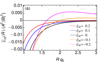
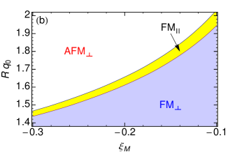
Figure 3: (a) Intrinsic real-space spin susceptibility $\overline{\chi}_{zz}(R)$ plotted as a function of $R\,q_{0}$ for several values of the gap parameter $\xi_{\text{M}}$, with fixed $\xi_{\text{D}}=-0.7$ and $\gamma=-2.22$. (b) Parameter domains of preferential alignments between localized Mn spins having a distance $R$, mediated by the intrinsic spin response of an HgTe quantum-well system. The blue (white) domain favours a ferromagnetic (anti-ferromagnetic) out-of-plane spin alignment. In the yellow region the two localized spins tend to align ferromagnetically in-plane.

Having considered the case of two localized impurity spins with exchange interactions mediated by virtual excitations, we now focus on a HgTe quantum well that is doped with a large number of homogeneously distributed magnetic impurities (eg, Mn ions), forming effectively a Hg_1-xMn_xTe alloy Lewiner and Bastard (1980). The average distance between the spins is $R_{\text{NN}}\approx(3a^{3}_{0}/16\pi x)^{1/3}$ Litvinov and Dugaev (2001), with $a_{0}$ the HgTe lattice constant and $x$ the concentration of magnetic ions. We calculate the Curie temperature in the mean field limit, assuming $R_{\text{NN}}/R_{0}\ll 1$ which is justified when $x\gg 2\times 10^{-3}|\xi_{\text{M}}|^{3}$, where we have used $q_{0}\lesssim 0.5$ nm^-1. Since $|\xi_{\text{M}}|\lesssim 0.3$ Mühlbauer et al. (2014), this condition is practically always fulfilled. The Curie temperature for Ising-type ferromagnetic order with magnetization perpendicular to the quantum well growth direction is given by

$$T_{\mathrm{C(i)}}=T_{0}~{}\frac{d_{\text{c}}/d(\xi_{\text{M}})}{1+4\xi_{\text{M}}\Theta(\xi_{\text{M}})}~{},$$ (12)

where $T_{0}=\frac{I(I+1){\mathcal{C}}^{2}_{z}(\gamma)}{48\pi}\frac{G^{2}}{k_{\text{B}}|B|}\frac{n_{I}}{d_{\text{c}}}$, $I$ denotes the impurity-spin magnitude, $n_{I}$ is the 3D density of magnetic impurities, and $d_{\text{c}}\approx 6.3$ nm is the critical well width. For obtaining Eq. (12) we have used the approximation $\int_{-d/2}^{d/2}dz\int_{-d/2}^{d/2}dz^{\prime}\chi^{(\text{int})}_{jj}(\gamma;0,z,z^{\prime})\approx\overline{\chi}^{(\text{int})}_{jj}(\gamma;0)$. In Fig. 1(a), we show the Curie temperature as a function of $\xi_{\text{M}}$, where we set $A=0.375$ eV nm and $B=-1.120$ eV nm² Mühlbauer et al. (2014) as their dependence on $d$ is much weaker compared to $M$. We see that the behavior of the Curie temperature in its dependence on $\xi_{\text{M}}$, or equivalently $d$, provides a clear means to distinguish between topological and normal regions.

Knowing the spin susceptibility as a function of the wave vector allows us to go beyond the mean field limit Simon and Loss (2007); Simon et al. (2008) and discuss the stability of the mean-field ground state with respect to thermally excited spin waves (magnons). In our present case of interest, the magnon dispersion for $q/q_{0}\ll 1$ is given by $\omega_{q}=\omega_{0}+c_{2}q^{2}$, with a coefficient $c_{2}=\left.\frac{1}{2}\frac{\partial^{2}\overline{\chi}^{(\text{int})}_{zz}(\gamma;q)}{\partial q^{2}}\right|_{q=0}$. Using Figure 6 in Appendix A, which shows results for the relevant set of parameters, we find $c_{2}\lesssim 0$. Thus the criterion Yosida (1996); Simon et al. (2008); Kernreiter et al. (2013) $c_{2}>0$ needed to guarantee stability of the mean-field ground state is generally violated. It may be possible that electron-electron interactions and/or spin-orbit coupling help to stabilize ferromagnetic order, as has been shown to be the case for an ordinary 2D electron gas Simon and Loss (2007); Simon et al. (2008); Żak et al. (2012), but this question is beyond the scope of our present work.

III.2 Spin response of the electron-doped system

We consider now situations where the conduction band is occupied ($\mu>E_{0}|\xi_{\text{M}}|$). In the $q\to 0$ limit, an analytical expression for the extrinsic contribution to the spin susceptibility (arising from filled conduction-band states) is found as

$$\overline{\chi}_{xx}^{(\text{dop})}(\gamma;0) = \frac{\mathcal{C}^{2}_{x}(\gamma)}{16\pi|B|}\Biggl{[}\frac{2\pi\tilde{N}(0)}{f^{2}}\Big{(}\tilde{k}_{\text{F}}^{2}-2f(\tilde{k}_{\text{F}}^{2}+\xi_{\text{M}})-\,2f^{2}\Big{)}+\frac{\tilde{k}_{\text{F}}^{2}(1+2\xi_{\text{M}})+2\xi_{\text{M}}^{2}-2f|\xi_{\text{M}}|)}{f(1+4\xi_{\text{M}})}\Biggr{]}~{},$$ (13a)

$$\overline{\chi}_{zz}^{(\text{dop})}(\gamma;0) = \frac{\mathcal{C}^{2}_{z}(\gamma)}{16\pi|B|}\Biggl{[}\frac{2\pi\tilde{N}(0)}{f^{2}}\left(\frac{6\gamma\mathcal{D}_{z}(\gamma)}{\mathcal{C}^{2}_{z}(\gamma)}\,\tilde{k}_{\text{F}}^{2}-\frac{4f^{2}\{\mathcal{D}^{2}_{z}(\gamma)(\tilde{k}_{\text{F}}^{2}+\xi_{\text{M}}+f)^{4}+9\gamma^{2}\tilde{k}_{\text{F}}^{4}\}}{\mathcal{C}^{2}_{z}(\gamma)[\tilde{k}_{\text{F}}^{2}+(\tilde{k}_{\text{F}}^{2}+\xi_{\text{M}}+f)^{2}]^{2}}\right)+\frac{\tilde{k}_{\text{F}}^{2}(1+2\xi_{\text{M}})+2\xi_{\text{M}}^{2}-2f|\xi_{\text{M}}|)}{f(1+4\xi_{\text{M}})}\Biggr{]}~{},$$

where the first (second) term between the square brackets in the expression for $\overline{\chi}_{jj}^{(\text{dop})}(\gamma;0)$ is an intraband (interband) contribution. In Eqs. (13), we used the abbreviations $\mathcal{D}_{z}(\gamma)\equiv(1-\gamma)\,\mathcal{C}_{\text{LH}}-1$ and $f\equiv\sqrt{(\tilde{k}_{\text{F}}^{2}+\xi_{\text{M}})^{2}+\tilde{k}_{\text{F}}^{2}}$. $\tilde{N}(0)$ is related to the density of states at the Fermi energy as $-\overline{\chi}_{0}(0)=N(0)=(2/|B|)~{}\tilde{N}(0)$ (where $\overline{\chi}_{0}(q)$ is the static charge-response function), and reads $\tilde{N}(0)=\frac{1}{2\pi}\left|\frac{1+2\tilde{k}_{\text{F}}^{2}+2\xi_{\text{M}}}{\sqrt{(\tilde{k}_{\text{F}}^{2}+\xi_{\text{M}})^{2}+\tilde{k}_{\text{F}}^{2}}}-2\xi_{\text{D}}\right|^{-1}$. For the general case with $q>0$, $\overline{\chi}_{jj}(\gamma;q)$ can be calculated numerically and its line shape is presented in Appendix C for various examples. Due to the sharpness of the Fermi surface, we find for the corresponding real-space spin susceptibilities the expected $R^{-2}$ oscillatory decay expected from a 2D Fermi liquid Giuliani and Vignale (2005).

Next we calculate the Curie temperature using the mean field approach under the premise $k_{\text{F}}R_{\text{NN}}\ll 1$, which leads to the condition $x\gg 2\times 10^{-3}~{}\tilde{k}_{\text{F}}$. This condition is generally fulfilled since $k_{\text{F}}\lesssim 0.1$ nm^-1 is the reliable range of the effective model Mühlbauer et al. (2014). The Curie temperature is given by

$$T_{\mathrm{C(d)}}=T_{0}~{}\frac{d_{\text{c}}}{d(\xi_{\text{M}})}~{}\frac{16\pi|B|}{C^{2}_{z}(\gamma)}~{}|\overline{\chi}_{zz}(\gamma;0)|~{},$$ (14)

where $\overline{\chi}_{zz}(\gamma;0)=\overline{\chi}^{(\text{int})}_{zz}(\gamma;0)+\overline{\chi}^{(\text{dop})}_{zz}(\gamma;0)$. Note that also in the doped case Ising type magnetism prevails. In Fig. 1(b), we show the Curie temperature as a function of $\xi_{\text{M}}$ for various values of the Fermi wave vector. For low doping, we see a strong dependence of the Curie temperature on $\xi_{\text{M}}$ in the topological regime, which becomes very weak in the normal regime. For large doping, on the other hand, the Curie temperature is not very sensitive to $\xi_{\text{M}}$ in its whole range. Furthermore, the Curie temperature is generally suppressed with increased doping, but this trend is much stronger in the topological regime. For the doped case, we find the magnon dispersion $\omega_{q}=\omega_{0}+\bar{c}_{2}q^{2}$ where $\bar{c}_{2}\equiv\frac{1}{2}\left.\frac{\partial^{2}\overline{\chi}_{zz}(\gamma;q)}{\partial q^{2}}\right|_{q=0}>0$ always, in contrast to the intrinsic case. See Fig. 8 in Appendix C. Thus a necessary condition for the stability of the ferromagnetic groundstate is fulfilled Yosida (1996); Simon et al. (2008); Kernreiter et al. (2013).

IV Confinement dependence of the 2D-electron effective $\mathbf{g}$ factor

The paramagnetic response of charge carriers in quantum-confined structures is usually interpreted in terms of the Pauli spin susceptibility and quantified by an effective single-particle $g$ factor Tutuc et al. (2002); Zhu et al. (2003); Shashkin et al. (2006). However, any actually measured spin-related quantities correspond almost always to averaged collective responses of the, e.g., quasi-2D, electron system that can be crucially affected by nontrivial spin-related phenomena Kernreiter et al. (2013). Here we consider the paramagnetic response of conduction-band electrons in HgTe quantum wells and show how their paramagnetic response is changed as a function of the band-gap parameter that drives the transition between the topological and normal regimes.

To define an effective $g$-factor for our system of a HgTe quantum well, we introduce the bulk-material Zeeman term $\mathscr{H}_{{\bm{\mathrm{\mathcal{B}}}}}=g_{\ast}\,\mu_{\text{B}}\sum_{j}{\mathcal{B}}_{j}\,\hat{S}_{j}(-2\kappa/g_{\ast})$, where $\mu_{\text{B}}$ is the Bohr magneton and $g_{\ast}$ ($\kappa$) the $\Gamma_{6}$-band ($\Gamma_{8}$-band) $g$ factor Winkler (2003). Linear-response theory enables us to determine the paramagnetic response to the magnetic field, which is given by $\overline{\chi}_{\text{P},j}=(g_{\ast}\mu_{\text{B}})^{2}\,\overline{\chi}^{(\text{dop})}_{jj}(-2\kappa/g_{\ast};q)|_{q=0}$, where $\overline{\chi}_{jj}^{(\text{dop})}(-2\kappa/g_{\ast};q)$ are the spin susceptibilities of the electron doped system for the in-plane and out-of-plane response involving $\hat{S}_{j}(-2\kappa/g_{\ast})$, see Eq. (13) for $\gamma=-2\kappa/g_{\ast}$. We compare this with the Pauli susceptibility given by $\overline{\chi}_{\text{P},j}=(g_{j}\mu_{\text{B}})^{2}~{}\overline{\chi}_{0}(0)/4$, with $\overline{\chi}_{0}(0)$ being (up to a minus sign) the density of states which is the zero-$q$ limit of the Lindhard function and $g_{j}$ is the Landé $g$-factor for the two directions. Thus, we can extract collective $g$ factors for the charge carriers as

$$g_{j}=g_{\ast}\,\,\sqrt{\left.4\,\,\frac{\overline{\chi}^{(\text{dop})}_{jj}(-2\kappa/g_{\ast};q)}{\overline{\chi}_{0}(q)}\right|_{q=0}}\quad.$$ (15)

Our approach to determine $g$ factors via the spin susceptibility complements previous work König et al. (2008) where an effective Zeeman term was derived for the BHZ Hamiltonian.

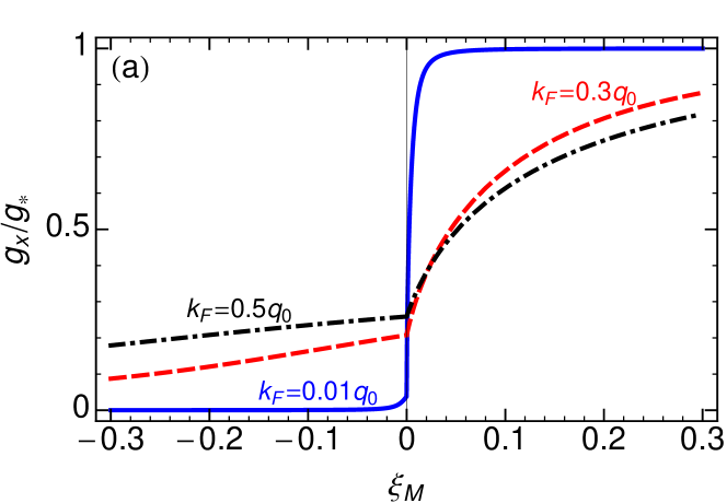
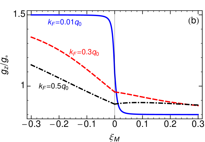
Figure 4: Effective $g$-factors associated with (a) the in-plane and (b) the out-of-plane response of an electron-doped HgTe quantum well, plotted as a function of the gap parameter $\xi_{\text{M}}$ for various levels of doping and with $\xi_{\text{D}}=-0.7$, $2\kappa/g_{\ast}=-0.5$. (Note that $k_{\mathrm{F}}=q_{0}$ corresponds to a charge density $n_{0}\equiv q_{0}^{2}/(2\pi)=4.25\times 10^{12}\,$cm^-2 for a typical structure Rothe et al. (2010).)

For a narrow-gap semiconductor, the values for $g_{\ast}$ and $\kappa$ are dominated by band-coupling contributions. Using generic expressions resulting from Kane-model descriptions Winkler (2003), we find

$$\frac{2\kappa}{g_{\ast}}=-\frac{\xi_{M}+\xi_{\Delta}}{2\xi_{\Delta}}\quad,$$ (16)

with $\xi_{\Delta}=\Delta_{0}\,|B|/A^{2}$ in terms of the spin-orbit-splitting gap $\Delta_{0}$ between the $\Gamma_{8}$ and $\Gamma_{7}$ band edges in the $8\times 8$ Kane model. As $\xi_{\Delta}\gg|\xi_{M}|$ for our situations of interest, we can set $2\kappa/g_{\ast}\to-0.5$ in the following. Hence, in Fig. 4, we show the effective $g$-factors for in-plane and out-of-plane responses as a function of $\xi_{\text{M}}$ for various levels of electron doping obtained for $2\kappa/g_{\ast}=-0.5$.

For very low densities, we see a vanishing in-plane response and a maximal $g_{z}=6\kappa$ HH-like out-of-plane response in the topological region $\xi_{\text{M}}<0$. This behavior arises because the conduction-band character is dominated by the HH basis states, which experience a “frozen” spin orientation perpendicular to the quantum well due to the confinement-induced HH-LH energy splitting Winkler et al. (2008). This can be easily verified from (13) by taking the limit $k_{\text{F}}\to 0$. Departures from these results occur for larger doping levels (larger $k_{\text{F}}$) due to increased HH-LH mixing. In the normal region ($\xi_{\text{M}}>0$), we encounter the situation that the conduction band is dominantly composed of the electron basis states, rendering the g factor to be sizable at any doping. The fact that the in-plane spin response is notably larger than the out-of-plane response for $\xi_{\text{M}}>0$ and low doping is due to the LH admixture in the conduction-band states. As the carrier density increases, the concomitantly increased HH-LH mixing results in significant modifications. More detailed exploration of parametric dependences exhibited by the collective g factors obtained here will be useful to augment previous perturbative estimates König et al. (2008) and aid the interpretation of recent measurements Hart et al. .

V Spin response of quasi-1D helical edge states in the topological regime

We have also investigated the edge-state contributions to the spin susceptibility in the topological region, finding them to be negligible compared to the bulk contributions in almost all situations. The only exception occurs for the in-plane response function $\overline{\chi}_{xx}(\gamma;q)$ in the purely intrinsic situation where the Fermi level lies in the minigap of the edge-state dispersions that opens up in a finite-size sample Zhou et al. (2008); Qi and Zhang (2011). More details and full results pertaining to edge states are given in Appendices D and E.

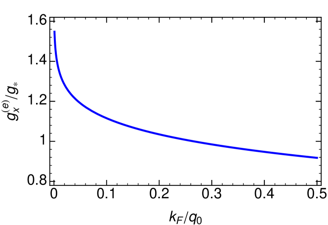
Figure 5: Effective $g$-factor characterising the response of helical edge states to an in-plane magnetic field.

Upto very small finite-size corrections, the paramagnetic response of helical edge states is captured by using the effective $g$-factors $g^{(\text{e})}_{x,z}$ given by

$$\frac{g^{(\text{e})}_{x}}{g_{\ast}} = \sqrt{\frac{\mathcal{C}^{2}_{x}(-2\kappa/g_{\ast})}{4}\,\,\ln\left(\frac{\Lambda}{k_{\text{F}}}\right)}\,\,\stackrel{{\scriptstyle\frac{2\kappa}{g_{\ast}}=-\frac{1}{2}}}{{\longrightarrow}}\,\,\frac{\sqrt{\ln\left(\frac{\Lambda}{k_{\text{F}}}\right)}}{2}~{},$$

$$\frac{g^{(\text{e})}_{z}}{g_{\ast}} = -\frac{4\kappa}{g_{\ast}}+\frac{1-{\mathcal{C}}_{\mathrm{LH}}}{2}\left(1+\frac{2\kappa}{g_{\ast}}\right)\,\,\stackrel{{\scriptstyle\frac{2\kappa}{g_{\ast}}=-\frac{1}{2}}}{{\longrightarrow}}\,\,1+\frac{1-{\mathcal{C}}_{\mathrm{LH}}}{4}\,.$$

The results shown in Eqs. (17) were obtained using Eq. (15) together with Eqs. (33a)-(33b). The prediction of the edge-state g factor is a major result of our work. In Fig. 5, we plot the in-plane $g$-factor as a function of $k_{\text{F}}$ where we used the natural cut-off scale $\Lambda=\pi/a_{0}$. Interestingly, the in-plane $g$-factor of edge states decreases monotonically with increasing doping level. Such a behavior is in stark contrast to the bulk case shown in Fig. 4(a) and to other 2D systems Kernreiter et al. (2013); Hatami et al. (2014) where the in-plane response increases with increased doping. This behavior reflects the fact that the spin-quantisation axis of the edge states is perpendicular to the 2D plane, i.e., parallel to the $z$ direction, and their helical nature.

VI Conclusions

We present a detailed theoretical study of the spin response in HgTe quantum wells where virtual-carrier-related processes are particularly relevant and exactly tractable within the effective BHZ-model description. Anomalous properties of the spin susceptibility and carrier-mediated magnetism are found in the inverted regime, extending our current understanding of spin-related properties in topological materials.

Most strikingly, the uniform static spin susceptibility in the intrinsic limit is constant, independent of the band gap, in the topological regime [see Eq. (1)]. This results in a distinct asymmetry between normal and inverted systems illustrated, e.g., by the dependence of the critical temperature for virtual-carrier-mediated magnetic order in a system that is doped with magnetic ions. Important differences between the two regimes are also exhibited in the situation where the conduction band becomes filled (see Fig. 1). The stability of mean-field ferromagnetic ground states with respect to thermal excitations of magnons has been analysed. We find that the magnetic order is stable in the situation with finite doping.

In the topological regime, quasi-1D helical edge states exist. We have investigated their spin-response properties, finding that their contribution to the spin susceptibility is thermodynamically suppressed compared to that arising from 2D quantum-well states, except in the very special – and probably physically hard-to-realise – situation when the chemical potential is in the mini-gap opened by the hybridisation of states from opposite edges in a finite sample.

We have used our results obtained for the spin susceptibility to define effective collective $g$ factors for states from the quasi-2D quantum-well subbands and also for the quasi-1D helical edge states. The different character of quasi-2D-subband states in the normal and topological (inverted) regimes is reflected in the values for the effective $g$ factor. Their strong dependence on charge-carrier density reveals the importance of interband mixing. The behavior of the $g$ factors found for the edge states reflects their helical nature and spin-quantization property.

Our results are directly relevant for current and potential future experimental investigations of the spin-related properties of 2D topological insulators, in particular those realised in HgTe/HgCdTe and InAs/GaSb quantum wells. For example, recent observation of Josephson-junction interference patterns in an S-HgTe/HgCdTe-S hybrid system has enabled extraction of g factors for the quantum-well charge carriers Hart et al. . It would be interesting to use similar techniques Hart et al. (2014); Pribiag et al. (2015) to measure the edge-state g factors and compare with our predictions. Furthermore, our results for the spin response in both the intrinsic and doped regimes are informative for the design of, and interpretation of measured quantities for, dilute magnetic phases in these systems Novik et al. (2005); Dietl (2010).

It would be interesting to extend our formalism to study the spin response in 3D topological-insulator materials Hasan and Moore (2011). In particular, as was the case in the 2D quantum-well-based TIs considered in this work, the interplay of charge-carrier dynamics and the spinor character of extended bulk states could be a source of rich variety in spin-related properties also in 3D, and the contributions of the conducting surfaces are currently not understood.

Appendix A Intrinsic contribution to the spin susceptibility

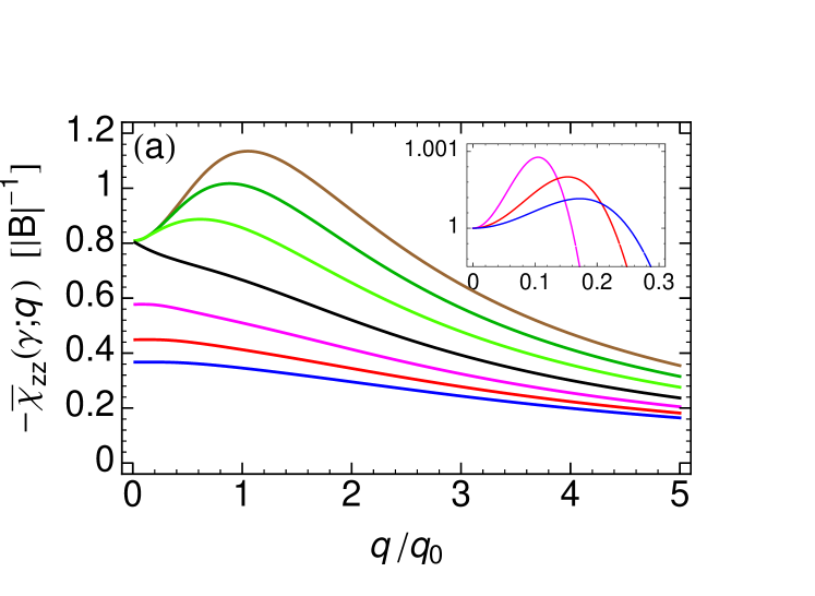
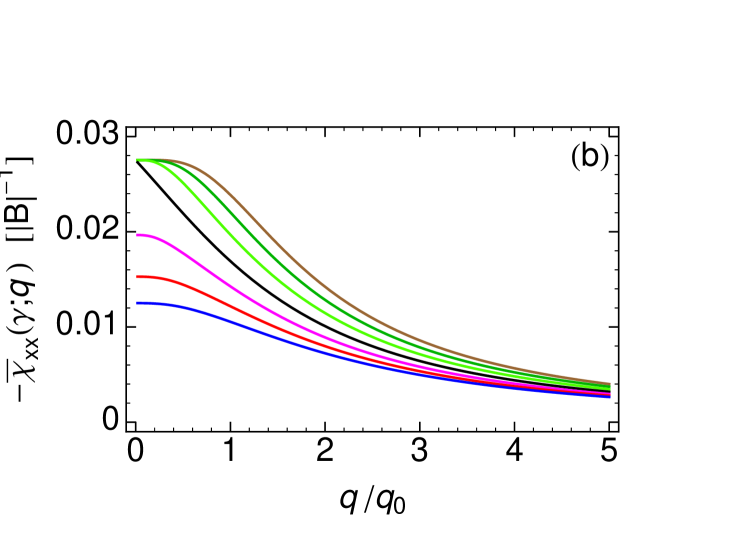
Figure 6: Intrinsic spin susceptibilities (a) $\overline{\chi}_{zz}(\gamma;q)$ and (b) $\overline{\chi}_{xx}(\gamma;q)$ as a function of $q/q_{0}$ for various values of $\xi_{\text{M}}=(-0.3,-0.2,-0.1,0,0.1,0.2,0.3)$ (from top to bottom) with $\xi_{\text{D}}=-0.7$, $\mathcal{C}_{\text{LH}}=0.4$ and $\gamma=-2.22$. The inset in (a) displays the normalized spin susceptibility $\overline{\chi}_{zz}(\gamma;q)/\overline{\chi}_{zz}(\gamma;0)$ in the small $q/q_{0}$ region for $\xi_{\text{M}}=(0.1,0.2,0.3)$, which shows more clearly that $\overline{\chi}_{zz}(\gamma;q)>\overline{\chi}_{zz}(\gamma;0)$ in the small-$q$ limit also in the normal regime.

The intrinsic contributions to the diagonal entries of the spin susceptibility (the only ones that are non-zero for the BHZ model) are calculated by

$$\overline{\chi}_{jj}^{(\text{int})}(\gamma;{\bm{\mathrm{q}}}) = -\sum_{s,s^{\prime}\atop\delta=\pm 1}\int\frac{d^{2}k}{(2\pi)^{2}}~{}~{}\frac{\mathscr{W}_{jj({\bm{\mathrm{k}}},{\bm{\mathrm{k}}}+{\bm{\mathrm{q}}},+,-)}^{(s,s^{\prime})}(\gamma)~{}n_{\text{F}}\big{(}E^{(s)}_{{\bm{\mathrm{k}}}-}\big{)}}{E^{(s)}_{{\bm{\mathrm{k}}}+}-E^{(s^{\prime})}_{{\bm{\mathrm{k}}}+{\bm{\mathrm{q}}}-}+i\hbar\eta\delta}~{},$$

where in the zero-temperature limit the valence band is fully occupied, i.e., $n_{\text{F}}\big{(}E^{(s)}_{{\bm{\mathrm{k}}}-}\big{)}=1$. Here and in the following we consider the growth-direction-averaged case: $\overline{\chi}_{ij}(\gamma;{\bm{\mathrm{q}}})=\int dz\int dz^{\prime}~{}\chi_{ij}(\gamma;{\bm{\mathrm{q}}};z,z^{\prime})\Rightarrow\mathscr{W}_{jj({\bm{\mathrm{k}}},{\bm{\mathrm{k}}}+{\bm{\mathrm{q}}},\alpha,\beta)}^{(s,s^{\prime})}(\gamma)=\int dz~{}dz^{\prime}~{}\mathscr{W}_{jj({\bm{\mathrm{k}}},{\bm{\mathrm{k}}}+{\bm{\mathrm{q}}},\alpha,\beta)}^{(s,s^{\prime})}(\gamma;z,z^{\prime})$. In Fig. 6, we plot $\overline{\chi}_{zz}(\gamma;q)$ [$\overline{\chi}_{xx}(\gamma;q)$] in panel (a) [(b)] as a function of $q$ for various values of $\xi_{\text{M}}$. The inset in Fig. 6(a) illustrates that $\left.\frac{\partial^{2}\overline{\chi}^{(\text{int})}_{zz}(\gamma;q)}{\partial q^{2}}\right|_{q=0}<0$ for all of the values of $\xi_{\text{M}}$ considered, which implies that the mean-field ferromagnetic order for out-of-plane aligned magnetic impurity spins will generally be destroyed by spin-wave (magnon) excitations Simon et al. (2008).

Appendix B Bloembergen-Rowland behavior of the local intrinsic spin susceptibility

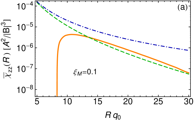
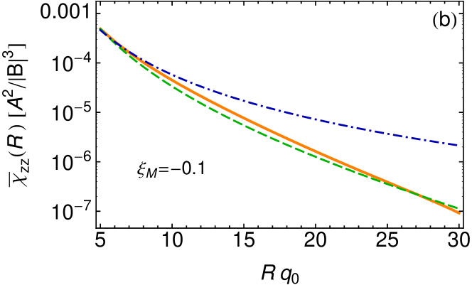
Figure 7: Local intrinsic spin susceptibilities $\overline{\chi}_{zz}(R)$ (solid orange curve) as a function of $Rq_{0}$ for (a) $\xi_{\text{M}}=0.1$ and (b) $\xi_{\text{M}}=-0.1$ with $\xi_{\text{D}}=-0.7$, $\mathcal{C}_{\text{LH}}=0.4$ and $\gamma=-2.22$. The dashed green curve shows the modelled behavior in Eq. (19) with coefficients $c=1$ for (a) and $c=1.2$ for (b). For comparison we also show the $R^{-3}$ decay for a gapless Dirac system represented by the dot-dashed blue curve. The sharp drop of the orange curve in (a) is due to a sign change of $\overline{\chi}_{zz}(R)$ at about $Rq_{0}\approx 8$.

Bloembergen and Rowland Bloembergen and Rowland (1955) found that the local RKKY interaction of gapped systems becomes short-ranged, i.e., is exponentially suppressed by the band-gap. The functional dependence of the local spin susceptibility on the distance for the gapped Dirac system at hand can thus be modelled by

$$\overline{\chi}_{jj}(R)\sim\frac{\mathrm{e}^{-c\frac{R}{\lambda_{\text{C}}}}}{R^{3}}~{},$$ (19)

where $\lambda^{-1}_{\text{C}}\equiv|\xi_{\text{M}}|q_{0}$ is the inverse of the Compton wavelength of the system and $c\sim\mathcal{O}(1)$ is a numerical coefficient that can depend on the distance itself. To illustrate this behavior for the HgTe quantum well system, we plot $\overline{\chi}_{zz}(R)$ in Fig. 7 as a function of $Rq_{0}$ for $\xi_{\text{M}}=0.1$ [$\xi_{\text{M}}=-0.1$] in panel (a) [(b)] together with both the line shape expected for 2D massless-Dirac particles and the Bloembergen-Rowland result.

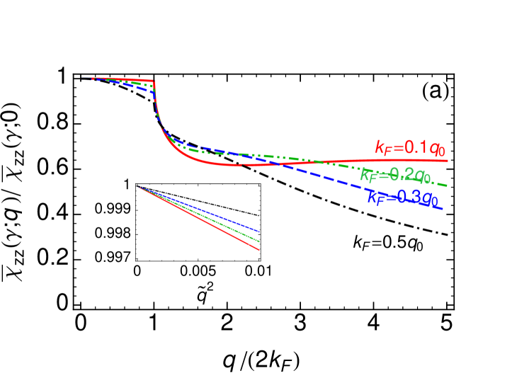
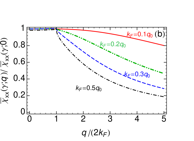
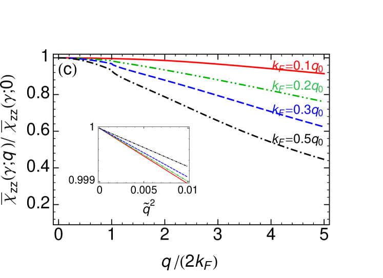
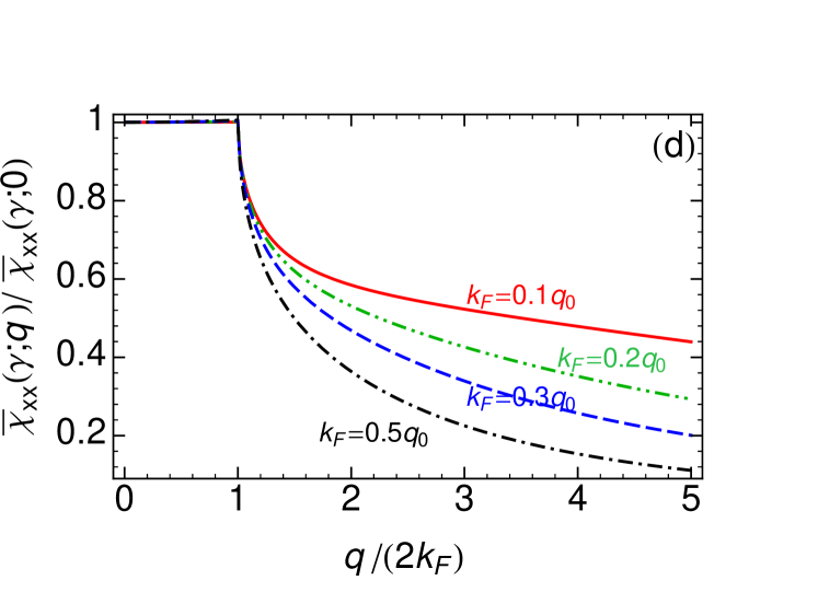
Figure 8: Normalized spin susceptibilities $\overline{\chi}_{zz}(\gamma;q)$ (a,c) and $\overline{\chi}_{xx}(\gamma;q)$ (b,d) as a function of $q/(2k_{\text{F}})$ for various levels of doping. (a,b) are the results for $\xi_{\text{M}}=-0.2$ and (c,d) for $\xi_{\text{M}}=0.2$, with $\xi_{\text{D}}=-0.7$, $\mathcal{C}_{\text{LH}}=0.4$ and $\gamma=-2.22$. The insets of (a,c) show the quadratic $\tilde{q}=q/q_{0}$ dependence close to $q=0$.

Appendix C Electron doped contribution to the spin susceptibility

For the case where the Fermi energy is above the conduction energy band edge, i.e., $\mu>|M|$, the spin susceptibility receives contributions due to electron doping given by

$$\overline{\chi}_{jj}^{(\text{dop})}(\gamma;{\bm{\mathrm{q}}}) = \sum_{s,s^{\prime}\atop\delta=\pm 1}\int\frac{d^{2}k}{(2\pi)^{2}}~{}n_{\text{F}}\big{(}E^{(s)}_{{\bm{\mathrm{k}}}+}\big{)}$$

$$\times\left[\frac{\mathscr{W}_{jj({\bm{\mathrm{k}}},{\bm{\mathrm{k}}}+{\bm{\mathrm{q}}},+,+)}^{(s,s^{\prime})}(\gamma)}{E^{(s)}_{{\bm{\mathrm{k}}}+}-E^{(s^{\prime})}_{{\bm{\mathrm{k}}}+{\bm{\mathrm{q}}}+}+i\hbar\eta\delta}+\frac{\mathscr{W}_{jj({\bm{\mathrm{k}}},{\bm{\mathrm{k}}}+{\bm{\mathrm{q}}},+,-)}^{(s,s^{\prime})}(\gamma)}{E^{(s)}_{{\bm{\mathrm{k}}}+}-E^{(s^{\prime})}_{{\bm{\mathrm{k}}}+{\bm{\mathrm{q}}}-}+i\hbar\eta\delta}\right],$$

where for zero temperature $n_{\text{F}}\big{(}E^{(s)}_{{\bm{\mathrm{k}}}+}\big{)}=\Theta\big{(}k_{\text{F}}-|{\bm{\mathrm{k}}}|\big{)}$, with $k_{\text{F}}$ being the Fermi wave vector associated with the conduction band. The complete spin susceptibility in the doped case is therefore given by

$$\overline{\chi}_{jj}(\gamma;{\bm{\mathrm{q}}})=\overline{\chi}_{jj}^{(\text{int})}(\gamma;{\bm{\mathrm{q}}})+\overline{\chi}_{jj}^{(\text{dop})}(\gamma;{\bm{\mathrm{q}}})~{}.$$ (21)

We show the line shape of $\overline{\chi}_{zz}(\gamma;q)$ and $\overline{\chi}_{xx}(\gamma;q)$ in Fig. 8 for $\xi_{\text{M}}=\pm 0.2$ and various choices of doping. The insets of Fig. 8(a,c) show the small $q$ dependence of $\overline{\chi}_{zz}(\gamma;q)$, indicating the stability of the out-of-plane Ising-type ferromagnetism with respect to Magnon excitations.

Appendix D Combining bulk and edge contributions to the spin susceptibility

In order to compare bulk and edge contributions to the spin susceptibility we begin by considering the real-space spin-response function

$$\chi_{ij}({\bm{\mathrm{r}}},{\bm{\mathrm{r^{\prime}}}})=-\frac{i}{\hbar}\int_{0}^{\infty}dt\,\,\,\mathrm{e}^{-\eta t}\,\,\langle\left[S_{i}({\bm{\mathrm{r}}},t)\,,\,S_{j}({\bm{\mathrm{r^{\prime}}}},0)\right]\rangle\,\,,$$ (22)

where $S_{i}({\bm{\mathrm{r}}})=\Psi^{\dagger}({\bm{\mathrm{r}}})\hat{S}_{i}\Psi({\bm{\mathrm{r}}})$ are spin-density operators. In our system of interest, electrons shall be confined to move freely in $d<3$ dimensions, with system size $L$ in all of these free directions. The position vector shall be split up into a part ${\bm{\mathrm{R}}}$ comprising the coordinate directions in which the motion is free and a part ${\bm{\mathrm{\varrho}}}$ in whose coordinates motion is confined; ${\bm{\mathrm{r}}}=({\bm{\mathrm{R}}},{\bm{\mathrm{\varrho}}})$. The second-quantised electron operator in real-space representation can be written as

$$\Psi({\bm{\mathrm{r}}})=\sum_{{\bm{\mathrm{k}}},\alpha,s}\frac{\mathrm{e}^{i{\bm{\mathrm{k}}}\cdot{\bm{\mathrm{R}}}}}{\sqrt{L^{d}}}\,\,\psi^{(s)}_{{\bm{\mathrm{k}}}\alpha}({\bm{\mathrm{\varrho}}})\,\,c^{(s)}_{{\bm{\mathrm{k}}}\alpha}$$ (23)

with normalized spinor bound-state wave functions $\xi_{n{\bm{\mathrm{k}}}}({\bm{\mathrm{\varrho}}})$. A straightforward calculation yields

$$\chi_{ij}({\bm{\mathrm{r}}},{\bm{\mathrm{r^{\prime}}}})=\frac{1}{L^{d}}\,\sum_{\bm{\mathrm{q}}}\,\mathrm{e}^{i{\bm{\mathrm{q}}}\cdot({\bm{\mathrm{R}}}-{\bm{\mathrm{R^{\prime}}}})}\,\,\chi_{ij}^{(d\text{D})}({\bm{\mathrm{q}}};{\bm{\mathrm{\varrho}}},{\bm{\mathrm{\varrho^{\prime}}}})\quad,$$ (24a)

with the $${\bm{\mathrm{q}}} d d$$-dependent spin susceptibility of the -dimensional (D) system given by

$$\chi_{ij}^{(d\text{D})}({\bm{\mathrm{q}}};{\bm{\mathrm{\varrho}}},{\bm{\mathrm{\varrho^{\prime}}}}) = \sum_{\alpha,\beta,s,s^{\prime}}\,\frac{1}{L^{d}}\,\sum_{\bm{\mathrm{k}}}\mathscr{W}_{ij({\bm{\mathrm{k}}},{\bm{\mathrm{k}}}+{\bm{\mathrm{q}}},\alpha,\beta)}^{(s,s^{\prime})}({\bm{\mathrm{\varrho}}},{\bm{\mathrm{\varrho^{\prime}}}})$$ (24b)

$$\hskip 28.45274pt\times\,\frac{n_{\text{F}}(E^{(s)}_{{\bm{\mathrm{k}}}\alpha})-n_{\text{F}}(E^{(s^{\prime})}_{{\bm{\mathrm{k}}}+{\bm{\mathrm{q}}}\beta})}{E^{(s)}_{{\bm{\mathrm{k}}}\alpha}-E^{(s^{\prime})}_{{\bm{\mathrm{k}}}+{\bm{\mathrm{q}}}\beta}+i\hbar\eta}\,.\qquad$$

We are now interested in the homogeneous part of the spin response defined as

$$\Upsilon_{ij}=\int d^{3}r\,\,\int d^{3}r^{\prime}\,\,\,\,\chi_{ij}({\bm{\mathrm{r}}},{\bm{\mathrm{r^{\prime}}}})\equiv L^{d}\,\overline{\chi}_{ij}^{(d\text{D})}({\bm{\mathrm{q}}}=0)\quad,$$ (25a)

where

$$\overline{\chi}_{ij}^{(d\text{D})}({\bm{\mathrm{q}}})=\int d^{3-d}\varrho\,\,\int d^{3-d}\varrho^{\prime}\,\,\,\,\chi_{ij}^{(d\text{D})}({\bm{\mathrm{q}}};{\bm{\mathrm{\varrho}}},{\bm{\mathrm{\varrho^{\prime}}}})\quad.$$ (25b)

In the situation where both 2D bulk and 1D edge states are present, we therefore find

$$\Upsilon_{ij}=L^{2}\left[\overline{\chi}_{ij}^{(\text{2D})}({\bm{\mathrm{q}}}=0)+\frac{1}{L}\,\overline{\chi}_{ij}^{(\text{1D})}(q=0)\right]\quad.$$ (26)

Thus $L^{-2}\Upsilon$ is the well-defined quantity in the thermodynamic limit, and only those edge-related terms that scale with $L$ will contribute to it.

Appendix E Spin susceptibility of edge states

E.1 Spin susceptibility of edge states: Omitting finite size effects

Following Qi and Zhang (2011) (see also Zhou et al. (2008)), the dispersions for the edge states, using open boundary conditions for a confinement along the $x$ direction and assuming $D=0$, is given by

$$E^{(s)}_{k}=sAk~{},$$ (27)

where $k\equiv k_{y}$. The associated spinor wave functions are

$$\eta^{(s)}({\bm{\mathrm{\varrho}}}) = \sum_{l=1}^{2}\varphi^{(s)}_{0,l}(x)~{}\psi^{(s)}_{0l}(z)~{},$$ (28)

where $\varphi^{(s)}_{0}(x)=C(\mathrm{e}^{\lambda_{1}x}-\mathrm{e}^{\lambda_{2}x})\phi_{-s}$, with $\phi_{\pm}^{T}=(1,\pm i)$ and $\lambda_{1,2}=-\frac{q_{0}}{2}(1\pm\sqrt{1-4|\xi_{\text{M}}}|)$, since $M<0$. To simplify matters, we have assumed particle-hole symmetry ($D=0$) and the system length $L\to\infty$, i.e., the gap in the dispersions of the edge states is negligible. Note that the spinors in Eq. (28) are independent of the wave vector component along the $y$ direction.

The spin susceptibility of the edge states is calculated by

$$\chi^{\text{(edge)}}_{jj}(\gamma;q;{\bm{\mathrm{\varrho}}},{\bm{\mathrm{\varrho^{\prime}}}}) = \sum_{s,s^{\prime}}\int\frac{dk}{2\pi}~{}\mathscr{W}_{jj}^{(s,s^{\prime})}(\gamma;{\bm{\mathrm{\varrho}}},{\bm{\mathrm{\varrho^{\prime}}}})$$ (29)

$$\times\frac{n_{\text{F}}[E^{(s)}_{k}]-n_{\text{F}}[E^{(s^{\prime})}_{k+q}]}{E^{(s)}_{k}-E^{(s^{\prime})}_{k+q}+i\hbar\eta}~{},$$

where

$$\mathscr{W}_{jj}^{(s,s^{\prime})}(\gamma;{\bm{\mathrm{\varrho}}},{\bm{\mathrm{\varrho^{\prime}}}}) = [\eta^{(s)}({\bm{\mathrm{\varrho}}})]^{\dagger}\cdot\hat{S}_{j}(\gamma)\cdot\eta^{(s^{\prime})}({\bm{\mathrm{\varrho}}})$$ (30)

$$\times[\eta^{(s^{\prime})}({\bm{\mathrm{\varrho^{\prime}}}})]^{\dagger}\cdot\hat{S}_{j}(\gamma)\cdot\eta^{(s)}({\bm{\mathrm{\varrho^{\prime}}}}).$$

With an averaging over the coordinates along the confined directions we have

$$\int d{\bm{\mathrm{\varrho}}}~{}d{\bm{\mathrm{\varrho^{\prime}}}}~{}\mathscr{W}_{zz}^{(s,s^{\prime})}(\gamma;{\bm{\mathrm{\varrho}}},{\bm{\mathrm{\varrho^{\prime}}}}) = \frac{\Xi^{2}_{z}(\gamma)}{16}\begin{pmatrix}1&0\\ 0&1\end{pmatrix}~{},$$ (31)

$$\int d{\bm{\mathrm{\varrho}}}~{}d{\bm{\mathrm{\varrho^{\prime}}}}~{}\mathscr{W}_{xx}^{(s,s^{\prime})}(\gamma;{\bm{\mathrm{\varrho}}},{\bm{\mathrm{\varrho^{\prime}}}}) = \frac{\Xi^{2}_{x}(\gamma)}{16}\begin{pmatrix}0&1\\ 1&0\end{pmatrix}~{},$$ (32)

with $\Xi_{z}(\gamma)=1+3\gamma+(\gamma-1)\mathcal{C}_{\text{LH}}$ and $\Xi_{x}(\gamma)=1+(2\gamma-1)\mathcal{C}_{\text{LH}}\equiv{\mathcal{C}}_{x}(\gamma)$. Thus $\chi^{(\text{edge})}_{zz}(\gamma;q)\propto\chi^{(\text{edge})}_{0}(q)$, where $\chi^{(\text{edge})}_{0}(q)$ is the Lindhard function associated with the edge states. Explicit calculation of (29) yields

$$\chi_{zz}^{(\text{edge})}(\gamma;q) = -\frac{\Xi^{2}_{z}(\gamma)}{16\pi A}\equiv\frac{\Xi^{2}_{z}(\gamma)}{16}\,\chi^{(\text{edge})}_{0}(q)~{},$$ (33a)

$$\chi_{xx}^{(\text{edge})}(\gamma;q) = \frac{\Xi^{2}_{x}(\gamma)}{32\pi A}\ln\left(\frac{|q^{2}-4k^{2}_{\text{F}}|}{4\Lambda^{2}-q^{2}}\right)~{},$$ (33b)

where $\Lambda$ is a large-wave-vector cut-off. Due to the special energy dispersion Eq. (27), $\chi_{zz}^{(\text{edge})}(\gamma;q)$ is a constant (independent of $k_{\text{F}}$ and $q$). Clearly, for the hole doped case ($\mu<0$), the same result as in Eq. (33) is obtained due to the assumed particle-hole symmetry.

E.2 Spin susceptibility of edge states: Finite size effects included

Following Zhou et al. (2008), we now take into account the finite size of the system. As a result, edge states at the two sides that have the same spin can couple which results in a gapped spectrum of their energy dispersions.We assume the system size $L$ to be large and use an approximation of the wave functions in Zhou et al. (2008). Taking into account the various degrees of freedom of both system sides, we modify the approach of Qi and Zhang (2011), where the solutions for the wave functions read

$$\varphi^{(s)}_{\nu}(x)=\frac{1}{\sqrt{C}}\left(\mathrm{e}^{\lambda_{1}(\frac{L}{2}-s\nu x)}-\mathrm{e}^{\lambda_{2}(\frac{L}{2}-s\nu x)}\right)\phi_{-s\nu}~{},$$

where $C$ is a normalization constant and $\nu=\pm$ denotes the right- and left-mover. For non-zero wave vector $k$, we consider the matrix

$${\mathcal{H}_{\text{RL}}}=\begin{pmatrix}Ak&\Delta\\[5.69054pt] \Delta&-Ak\end{pmatrix}~{}$$ (35)

in the basis of right- and left-mover, where $\Delta$ is the induced gap which is a function of the system parameters Zhou et al. (2008). The energy dispersions of (35) are

$$E^{(s)}_{k\tau}=\tau\sqrt{(Ak)^{2}+\Delta^{2}}~{},$$ (36)

where $\tau=\pm$ labels the (spin-degenerate) conduction and valence bands, respectively. The associated eigenstates are

$$a^{(s)}_{k\tau}=\begin{pmatrix}\sqrt{\frac{E^{(s)}_{k\tau}+Ak}{2E^{(s)}_{k\tau}}}\\[8.53581pt] \tau\sqrt{\frac{E^{(s)}_{k\tau}-Ak}{2E^{(s)}_{k\tau}}}\end{pmatrix}~{}.$$ (37)

With this information, the spinors in Eq. (28) are modified to

$$\eta^{(s)}_{k\tau}({\bm{\mathrm{\varrho}}}) = \sum_{l=1}^{2}\sum_{\nu}a^{(s)}_{k\tau,\nu}~{}\varphi^{(s)}_{\nu,l}(x)~{}\psi^{(s)}_{0l}(z)~{},$$ (38)

Thus, for the present case, the spin susceptibility of the edge states is

$$\chi^{\text{(edge)}}_{jj}(\gamma;q;{\bm{\mathrm{\varrho}}},{\bm{\mathrm{\varrho^{\prime}}}}) = \sum_{\begin{subarray}{c}s,s^{\prime}\\ \tau,\tau^{\prime}\end{subarray}}\int\frac{dk}{2\pi}~{}\mathscr{W}_{jj(k,k+q,\tau,\tau^{\prime})}^{(s,s^{\prime})}(\gamma;{\bm{\mathrm{\varrho}}},{\bm{\mathrm{\varrho^{\prime}}}})$$ (39)

$$\times\frac{n_{\text{F}}[E^{(s)}_{k\tau}]-n_{\text{F}}[E^{(s^{\prime})}_{k+q\tau^{\prime}}]}{E^{(s)}_{k\tau}-E^{(s^{\prime})}_{k+q\tau^{\prime}}+i\hbar\eta}~{},$$

where

$$\mathscr{W}_{jj(k,k+q,\tau,\tau^{\prime})}^{(s,s^{\prime})} (\gamma;{\bm{\mathrm{\varrho}}},{\bm{\mathrm{\varrho^{\prime}}}}) =[\eta^{(s)}_{k\tau}({\bm{\mathrm{\varrho}}})]^{\dagger}\cdot\hat{S}_{j}(\gamma)\cdot\eta^{(s^{\prime})}_{k+q\tau^{\prime}}({\bm{\mathrm{\varrho}}})$$

$$\times[\eta^{(s^{\prime})}_{k+q\tau^{\prime}}({\bm{\mathrm{\varrho^{\prime}}}})]^{\dagger}\cdot\hat{S}_{j}(\gamma)\cdot\eta^{(s)}_{k\tau}({\bm{\mathrm{\varrho^{\prime}}}})~{}.$$

Averaging over the coordinates along the confined directions, we obtain for the overlap factor of the Lindhard function

$$\int d{\bm{\mathrm{\varrho}}}~{}d{\bm{\mathrm{\varrho^{\prime}}}}~{}\mathscr{W}_{0(k,k+q,\tau,\tau^{\prime})}^{(s,s^{\prime})}({\bm{\mathrm{\varrho}}},{\bm{\mathrm{\varrho^{\prime}}}})=\frac{\delta_{ss^{\prime}}}{4}$$

$${}\times\begin{cases}(a_{k}a_{k+q}+b_{k}b_{k+q})^{2}&\quad(\tau=\tau^{\prime})\\[8.53581pt] (a_{k}b_{k+q}-b_{k}a_{k+q})^{2}&\quad(\tau\neq\tau^{\prime})\end{cases}$$ (41)

where $a_{k}\equiv\sqrt{1-\frac{Ak}{\sqrt{(Ak)^{2}+\Delta^{2}}}}$, $b_{k}\equiv\sqrt{1+\frac{Ak}{\sqrt{(Ak)^{2}+\Delta^{2}}}}$. The result for the overlap factors of the spin susceptibilities is

$$\int d{\bm{\mathrm{\varrho}}}~{}d{\bm{\mathrm{\varrho^{\prime}}}}~{}\mathscr{W}_{zz(k,k+q,\tau,\tau^{\prime})}^{(s,s^{\prime})}(\gamma;{\bm{\mathrm{\varrho}}},{\bm{\mathrm{\varrho^{\prime}}}})=\frac{\delta_{ss^{\prime}}}{64}$$

$${}\times\begin{cases}[(a_{k}a_{k+q}+b_{k}b_{k+q})~{}\Xi_{z}(\gamma)&\quad(\tau=\tau^{\prime})\\[2.84526pt] +\tau(a_{k}b_{k+q}+b_{k}a_{k+q})~{}\mathcal{C}_{z}(\gamma)~{}NL\Delta]^{2}\\[8.53581pt] [(b_{k}b_{k+q}-a_{k}a_{k+q})~{}\mathcal{C}_{z}(\gamma)~{}NL\Delta&\quad(\tau\neq\tau^{\prime})\\[2.84526pt] +\tau(a_{k}b_{k+q}-b_{k}a_{k+q})~{}\Xi_{z}(\gamma)]^{2}\end{cases}$$ (42)

and

$$\int d{\bm{\mathrm{\varrho}}}~{}d{\bm{\mathrm{\varrho^{\prime}}}}~{}\mathscr{W}_{xx(k,k+q,\tau,\tau^{\prime})}^{(s,s^{\prime})}(\gamma;{\bm{\mathrm{\varrho}}},{\bm{\mathrm{\varrho^{\prime}}}})=\frac{\Xi^{2}_{x}(\gamma)}{64}(1-\delta_{ss^{\prime}})$$

$${}\times\begin{cases}[a_{k}b_{k+q}+b_{k}a_{k+q}&\quad(\tau=\tau^{\prime})\\[2.84526pt] +\tau(a_{k}a_{k+q}+b_{k}b_{k+q})NL\Delta]^{2}\\[8.53581pt] [a_{k}a_{k+q}-b_{k}b_{k+q}&\quad(\tau\neq\tau^{\prime})\\[2.84526pt] -\tau(a_{k}b_{k+q}-b_{k}a_{k+q})NL\Delta]^{2}\\[8.53581pt] \end{cases}$$ (43)

In obtaining (E.2)-(E.2) we have used

$$\int~{}dx\prod_{\nu}\left(\mathrm{e}^{\lambda_{1}(\frac{L}{2}-\nu x)}-\mathrm{e}^{\lambda_{2}(\frac{L}{2}-\nu x)}\right)\approx L~{}\mathrm{e}^{\lambda_{2}L}~{},$$ (44)

the functional $L$-dependence of $\Delta\approx F~{}\text{exp}(\lambda_{2}L)$ Zhou et al. (2008), where $F/E_{0}=4|\xi_{\text{M}}|/\sqrt{1-4|\xi_{\text{M}}|}$, and we have defined $N\equiv(FC)^{-1}$.

E.2.1 Intrinsic contribution to the spin susceptibilities of the edge states in the limit $q\to 0$

Calculating the intrinsic contribution to the spin susceptibilities of the edge states in the long-wavelength limit ($q\to 0$), we obtain

$$\chi^{(\text{int,e})}_{zz}(\gamma;0)=(NL\Delta)^{2}\frac{g_{\text{s}}\mathcal{C}^{2}_{z}(\gamma)}{16\pi A}\left[1-\ln\left(\frac{2\Lambda}{\tilde{\Delta}}\right)\right]~{},$$

$$\chi^{(\text{int,e})}_{xx}(\gamma;0)=\frac{g_{\text{s}}\Xi^{2}_{x}(\gamma)}{16\pi A}\left[1-\ln\left(\frac{2\Lambda}{\tilde{\Delta}}\right)\right]~{},$$ (45b)

where $\tilde{\Delta}\equiv\Delta/A$. We note that the intrinsic contribution to the Lindhard function vanishes in the limit $q\to 0$, which can be inferred from (E.2). To compare this result with the one of the intrinsic bulk contribution, we divide (45) and (45b) by the length $L$ and let $L$ go to infinity (see Sec. D). Thus, we obtain

$$\lim_{L\to\infty}\frac{\chi^{(\text{int,e})}_{zz}(\gamma;0)}{L}=0~{},$$ (46a)

$$\lim_{L\to\infty}\frac{\chi^{(\text{int,e})}_{xx}(\gamma;0)}{L}=-\frac{g_{\text{s}}\Xi^{2}_{x}(\gamma)}{32\pi|B|}\left(1-\sqrt{1-4|\xi_{\text{M}}|}\right)~{}.$$

Therefore, the edge states give a contribution to the total susceptibility only for the in-plane component and its sign equals that of the bulk contribution.

E.2.2 Electron doped contribution to the spin susceptibilities of the edge states in the limit $q\to 0$

Next we include the contributions due to doping to the spin susceptibilities. The interband contributions read (for $Ak_{\text{F}}\gg\Delta$)

$$\chi^{(\text{inter,e})}_{zz}(\gamma;0)=-(NL\Delta)^{2}\frac{g_{\text{s}}\mathcal{C}_{z}^{2}(\gamma)}{16\pi A}\left[1-\ln\left(\frac{2k_{\text{F}}}{\tilde{\Delta}}\right)\right],$$

$$\chi^{(\text{inter,e})}_{xx}(\gamma;0)=-\frac{g_{\text{s}}\Xi^{2}_{x}(\gamma)}{16\pi A}\left[1-\ln\left(\frac{2k_{\text{F}}}{\tilde{\Delta}}\right)\right],$$ (47b)

while the intraband contributions are

$$\chi^{(\text{intra,e})}_{zz}(\gamma;0)=-\frac{g_{\text{s}}\Xi^{2}_{z}(\gamma)}{16\pi A}~{},$$ (48a)

$$\chi^{(\text{intra,e})}_{xx}(\gamma;0)=-(NL\Delta)^{2}~{}\frac{g_{\text{s}}\Xi^{2}_{x}(\gamma)}{16\pi A}~{},$$ (48b)

which is consistent with the finding that $\chi^{(\text{intra,e})}_{zz}(\gamma;q)$ [$\chi^{(\text{intra,e})}_{xx}(\gamma;q)$] are important [unimportant] for $\Delta\to 0$, whereas it is the other way around for the interband contributions. Considering

$$\lim_{L\to\infty} \frac{[\chi^{(\text{intra,e})}_{zz}(\gamma;0)+\chi^{(\text{inter,e})}_{zz}(\gamma;0)]}{L}=0~{},$$ (49a)

$$\lim_{L\to\infty} \frac{[\chi^{(\text{intra,e})}_{xx}(\gamma;0)+\chi^{(\text{inter,e})}_{xx}(\gamma;0)]}{L}=$$ (49b)

$${}\hskip 39.83368pt\frac{g_{\text{s}}\Xi^{2}_{x}(\gamma)}{32\pi|B|}\left(1-\sqrt{1-4|\xi_{\text{M}}|}\right),$$

we find that this is the same contribution as the intrinsic contribution, Eq. (46), which has however the opposite sign. Thus, the sum of doped and intrinsic contributions of the edge states vanishes in the large $L$ limit. As a consistency check, we verify for $q=0$ that the sum of Eqs. (45), (47) and (48) yields Eqs. (33a) and (33b) (multiplied by $g_{\text{s}}$) in the limit $\Delta\to 0$.

Appendix F Effects of structural inversion asymmetry

Here we demonstrate that the basic features of the intrinsic spin susceptibilities given in Eq. (1) are robust even when effects due to structural inversion asymmetry (SIA) are included. By taking into account the influence of a perpendicular electric field $\mathcal{E}_{z}$, it has been shown in Ref. Rothe et al. (2010) that the BHZ Hamiltonian is supplemented by entries that mix the spin-up and spin-down components of the BHZ basis states. The leading contribution due to SIA is linear in the wave vector and given by

$$\mathscr{H}_{\text{R}}=\begin{pmatrix}0&0&-iR_{0}k_{-}&0\\[5.69054pt] 0&0&0&0\\[5.69054pt] iR_{0}k_{+}&0&0&0\\[5.69054pt] 0&0&0&0\end{pmatrix}~{},$$ (50)

where $k_{\pm}=k_{x}\pm ik_{y}$. The necessity to avoid dielectric breakdown provides an upper limit for the electric-field magnitude through the condition $|e\mathcal{E}_{z}|d<2|M|$. Defining the SIA-related dimensionless parameter $\xi_{\text{R}}\equiv R_{0}/A$, this condition translates into $|\xi_{\text{R}}|<16.1\,|\xi_{\text{M}}|/(d\,[\mbox{nm}])\approx 0.12$ for a typical heterostructure Rothe et al. (2010). Thus $\xi_{R}$ is generally a small parameter, and a perturbative treatment for SIA effects is appropriate. To lowest order in $\xi_{\text{R}}$, the intrinsic spin susceptibility in the limit $q\to 0$ is found as

$$\overline{\chi}^{(\text{int})}_{xx}(\gamma;{\bm{\mathrm{q}}}=0) = -\frac{\mathcal{C}^{2}_{x}(\gamma)}{16\pi|B|}\frac{1}{1+4\xi_{\text{M}}\Theta(\xi_{\text{M}})}\,\left(1+\xi_{\text{R}}^{2}~{}\frac{8\xi_{\text{M}}\Theta(\xi_{\text{M}})}{3[1+4\xi_{\text{M}}\Theta(\xi_{\text{M}})]^{2}}\right)~{},$$ (51a)

$$\overline{\chi}^{(\text{int})}_{zz}(\gamma;{\bm{\mathrm{q}}}=0) = -\frac{\mathcal{C}^{2}_{z}(\gamma)}{16\pi|B|}\frac{1}{1+4\xi_{\text{M}}\Theta(\xi_{\text{M}})}\,\left(1+\xi_{\text{R}}^{2}~{}\frac{2\{9\gamma^{2}+2\xi_{\text{M}}\Theta(\xi_{\text{M}})[\mathcal{C}^{2}_{z}(\gamma)+18\gamma^{2}]\}}{3\mathcal{C}^{2}_{z}(\gamma)[1+4\xi_{\text{M}}\Theta(\xi_{\text{M}})]^{2}}\right)~{}.$$ (51b)

Thus the lowest-order SIA corrections to $\overline{\chi}^{(\text{int})}_{jj}(\gamma;{\bm{\mathrm{q}}}=0)$ are quadratic in the small parameter $\xi_{\text{R}}$. This means that the result given in Eq. (51) represents already an excellent approximation. Interestingly, $\overline{\chi}^{(\text{int})}_{xx}(\gamma;{\bm{\mathrm{q}}}=0)$ turns out to not be modified by SIA contributions in the inverted regime. We find that this remains true even when higher-order corrections in $\xi_{\text{R}}$ are considered. In contrast, $\overline{\chi}^{(\text{int})}_{zz}(\gamma;{\bm{\mathrm{q}}}=0)$ in Eq. (51b) has finite SIA corrections in the inverted regime given by $6\gamma^{2}\xi_{\text{R}}^{2}/\mathcal{C}^{2}_{z}(\gamma)$. In our case where $\gamma=-2.22$ this amounts to a relative change that is about 1%. Also in the normal regime, SIA contributions to $\overline{\chi}^{(\text{int})}_{jj}(\gamma;{\bm{\mathrm{q}}}=0)$ are at most of relative magnitude 1%. Thus we conclude that the spin susceptibilities in Eq. (1) generally receive only very small corrections when SIA terms are included in the BHZ Hamiltonian.

References

- König et al. (2007) M. König, S. Wiedmann, C. Brüne, A. Roth, H. Buhmann, L. W. Molenkamp, X.-L. Qi, and S.-C. Zhang, “Quantum spin Hall insulator state in HgTe quantum wells,” Science 318, 766–770 (2007).
- Roth et al. (2009) A. Roth, C. Brüne, H. Buhmann, L. W. Molenkamp, J. Maciejko, X.-L. Qi, and S.-C. Zhang, “Nonlocal transport in the quantum spin Hall state,” Science 325, 294–297 (2009).
- Brüne et al. (2012) C. Brüne, A. Roth, H. Buhmann, E. M. Hankiewicz, L. W. Molenkamp, J. Maciejko, X.-L. Qi, and S.-C. Zhang, “Spin polarization of the quantum spin Hall edge states,” Nat. Phys. 8, 485–490 (2012).
- (4) S. Hart, H. Ren, M. Kosowsky, G. Ben-Shach, P. Leubner, C. Brüne, H. Buhmann, L. W. Molenkamp, B. I. Halperin, and A. Yacoby, “Controlled finite momentum pairing and spatially varying order parameter in proximitized HgTe quantum wells,” preprint arXiv:1509.02940.
- Qi and Zhang (2011) X.-L. Qi and S.-C. Zhang, “Topological insulators and superconductors,” Rev. Mod. Phys. 83, 1057–1110 (2011).
- Liu et al. (2008a) C. Liu, T. L. Hughes, X.-L. Qi, K. Wang, and S.-C. Zhang, “Quantum spin Hall effect in inverted type-II semiconductors,” Phys. Rev. Lett. 100, 236601 (2008a).
- Knez et al. (2011) I. Knez, R.-R. Du, and G. Sullivan, “Evidence for helical edge modes in inverted quantum wells,” Phys. Rev. Lett. 107, 136603 (2011).
- Hasan and Moore (2011) M. Z. Hasan and J. E. Moore, “Three-dimensional topological insulators,” Annu. Rev. Condens. Matter Phys. 2, 55–78 (2011).
- Lunde and Platero (2013) A. M. Lunde and G. Platero, “Hyperfine interactions in two-dimensional HgTe topological insulators,” Phys. Rev. B 88, 115411 (2013).
- Novik et al. (2005) E. G. Novik, A. Pfeuffer-Jeschke, T. Jungwirth, V. Latussek, C. R. Becker, G. Landwehr, H. Buhmann, and L. W. Molenkamp, “Band structure of semimagnetic quantum wells,” Phys. Rev. B 72, 035321 (2005).
- Liu et al. (2008b) C.-X. Liu, X.-L. Qi, X. Dai, Z. Fang, and S.-C. Zhang, “Quantum anomalous Hall effect in quantum wells,” Phys. Rev. Lett. 101, 146802 (2008b).
- Yu et al. (2010) R. Yu, W. Zhang, H.-J. Zhang, S.-C. Zhang, X. Dai, and Z. Fang, “Quantized anomalous Hall effect in magnetic topological insulators,” Science 329, 61–64 (2010).
- Simon and Loss (2007) P. Simon and D. Loss, “Nuclear spin ferromagnetic phase transition in an interacting two dimensional electron gas,” Phys. Rev. Lett. 98, 156401 (2007).
- Simon et al. (2008) P. Simon, B. Braunecker, and D. Loss, “Magnetic ordering of nuclear spins in an interacting two-dimensional electron gas,” Phys. Rev. B 77, 045108 (2008).
- Dietl (2010) T. Dietl, “A ten-year perspective on dilute magnetic semiconductors and oxides,” Nat. Mater. 9, 965–974 (2010).
- Giuliani and Vignale (2005) G. Giuliani and G. Vignale, Quantum Theory of the Electron Liquid (Cambridge U Press, Cambridge, UK, 2005).
- Kernreiter et al. (2013) T. Kernreiter, M. Governale, and U. Zülicke, “Carrier-density-controlled anisotropic spin susceptibility of two-dimensional hole systems,” Phys. Rev. Lett. 110, 026803 (2013).
- Liu et al. (2009) Q. Liu, C.-X. Liu, C. Xu, X.-L. Qi, and S.-C. Zhang, “Magnetic impurities on the surface of a topological insulator,” Phys. Rev. Lett. 102, 156603 (2009).
- Zhu et al. (2011) J.-J. Zhu, D.-X. Yao, S.-C. Zhang, and K. Chang, “Electrically controllable surface magnetism on the surface of topological insulators,” Phys. Rev. Lett. 106, 097201 (2011).
- Bernevig et al. (2006) B. A. Bernevig, T. L. Hughes, and S.-C. Zhang, “Quantum spin Hall effect and topological phase transition in HgTe quantum wells,” Science 314, 1757–1761 (2006).
- Kossut and Dobrowolski (1997) J. Kossut and W. Dobrowolski, “Properties of diluted magnetic semiconductors,” in Narrow Gap II-VI Compounds for Optoelectronic and Electromagnetic Applications, edited by P. Capper (Chapman & Hall, London, 1997) pp. 401–429.
- Rothe et al. (2010) D. G. Rothe, R. W. Reinthaler, C.-X. Liu, L. W. Molenkamp, S.-C. Zhang, and E. M. Hankiewicz, “Fingerprint of different spin-orbit terms for spin transport in HgTe quantum wells,” New J. Phys. 12, 065012 (2010).
- Mühlbauer et al. (2014) M. Mühlbauer, A. Budewitz, B. Büttner, G. Tkachov, E. M. Hankiewicz, C. Brüne, H. Buhmann, and L. W. Molenkamp, “One-dimensional weak antilocalization due to the Berry phase in HgTe wires,” Phys. Rev. Lett. 112, 146803 (2014).
- Juergens et al. (2014a) S. Juergens, P. Michetti, and B. Trauzettel, “Plasmons due to the interplay of Dirac and Schrödinger fermions,” Phys. Rev. Lett. 112, 076804 (2014a).
- Juergens et al. (2014b) S. Juergens, P. Michetti, and B. Trauzettel, “Screening properties and plasmons of Hg(Cd)Te quantum wells,” Phys. Rev. B 90, 115425 (2014b).
- Winkler (2003) R. Winkler, Spin-Orbit Coupling Effects in Two-Dimensional Electron and Hole Systems (Springer, Berlin, 2003).
- Note (1) For example, when discussing Pauli paramagnetism, the response function for with is relevant, where and are the respective factors for the and bands in the Kane-model band-structure description Winkler (2003). In contrast, the intrinsic real-spin polarisation is associated with . See, e.g., Eq. (6.65) in Ref. \rev@citealpWinkler2003Book. To discuss carrier-mediated magnetism, the susceptibility with in the notation of Ref. \rev@citealpDobrowolski needs to be considered. Finally, is the proper angular-momentum operator that generates spatial rotations.
- Note (2) For instance, for a perpendicular magnetic field , the grand canonical potential is given by , where and are the dispersions of the two spin-split bands () obtained from the effective Hamiltonian. In the limit (and ), we obtain . The net-magnetisation of the bands is given by . Numerically we find that , since the numerical coefficients of the two spin-split bands are related as .
- Note (3) In other words, while the total magnetic susceptibility of the HgTe quantum-well system is trivial (i.e., vanishes) in the intrinsic limit, the effective-spin susceptibility is finite and exhibits interesting properties that affect observable physical phenomena, e.g., impurity-spin exchange and Zeeman splitting; as discussed in the following.
- Note (4) The switching off of HH-LH mixing can be simulated by replacing in Eq. (2) and letting after integration.
- Zhou et al. (2010) L. Zhou, J. Wiebe, S. Lounis, E. Vedmedenko, F. Meier, S. Blügel, P. H. Dederichs, and R. Wiesendanger, “Strength and directionality of surface Ruderman-Kittel-Kasuya-Yosida interaction mapped on the atomic scale,” Nat. Phys. 6, 187–191 (2010).
- Khajetoorians et al. (2012) A. A. Khajetoorians, J. Wiebe, B. Chilian, S. Lounis, S. Blügel, and R. Wiesendanger, “Atom-by-atom engineering and magnetometry of tailored nanomagnets,” Nat. Phys. 8, 497–503 (2012).
- Yosida (1996) K. Yosida, Theory of Magnetism (Springer, Berlin, 1996).