BayesWipe: A Scalable Probabilistic Framework for Cleaning BigData

Abstract

Recent efforts in data cleaning of structured data have focused exclusively on problems like data deduplication, record matching, and data standardization; none of the approaches addressing these problems focus on fixing incorrect attribute values in tuples. Correcting values in tuples is typically performed by a minimum cost repair of tuples that violate static constraints like CFDs (which have to be provided by domain experts, or learned from a clean sample of the database). In this paper, we provide a method for correcting individual attribute values in a structured database using a Bayesian generative model and a statistical error model learned from the noisy database directly. We thus avoid the necessity for a domain expert or clean master data. We also show how to efficiently perform consistent query answering using this model over a dirty database, in case write permissions to the database are unavailable. We evaluate our methods over both synthetic and real data.

1 Introduction

Although data cleaning has been a long standing problem, it has become critically important again because of the increased interest in big data and web data. Most of the focus of the work on big data has been on the volume, velocity, or variety of the data; however, an important part of making big data useful is to ensure the veracity of the data. Enterprise data is known to have a typical error rate of 1–5% [1] (error rates of up to 30% have been observed). This has led to renewed interest in cleaning of big data sources, where manual data cleansing tasks are seen as prohibitively expensive and time-consuming [2], or the data has been generated by users and cannot be implicitly trusted [3]. Among the various types of big data, the need to efficiently handle large scaled structured data that is rife with inconsistency and incompleteness is also more significant than ever. Indeed, multiple studies, such as [4] emphasize the importance of effective, efficient methods for handling “dirty big data”.

TABLE I: A snapshot of car data extracted from cars.com using information extraction techniques

TID	Model	Make	Orig	Size	Engine	Condition
$t_{1}$	Civic	Honda	JPN	Mid-size	V4	NEW
$t_{2}$	Focus	Ford	USA	Compact	V4	USED
$t_{3}$	Civik	Honda	JPN	Mid-size	V4	USED
$t_{4}$	Civic	Ford	USA	Compact	V4	USED
$t_{5}$		Honda	JPN	Mid-size	V4	NEW
$t_{6}$	Accord	Honda	JPN	Full-size	V6	NEW

Most of the current techniques are based on deterministic rules, which have a number of problems: Suppose that the user is interested in finding ‘Civic’ cars from Table I. Traditional data retrieval systems would return tuples $t_{1}$ and $t_{4}$ for the query, because they are the only ones that are a match for the query term. Thus, they completely miss the fact that $t_{4}$ is in fact a dirty tuple — A Ford Focus car mislabeled as a Civic. Additionally, tuple $t_{3}$ and $t_{5}$ would not be returned as a result tuples since they have a typos or missing values, although they represent desirable results. The objective of this work is to provide the true result set ($t_{1},t_{3},t_{5}$) to the user.

Although this problem has received significant attention over the years in the traditional database literature, the state-of-the-art approaches fall far short of an effective solution for big data and web data. Traditional methods include outlier detection [5], noise removal [6], entity resolution [7, 6], and imputation [8]. Although these methods are efficient in their own scenarios, their dependence on clean master data is a significant drawback.

Specifically, state of the art approaches (e.g., [9, 10, 11]) attempt to clean data by exploiting patterns in the data, which they express in the form of conditional functional dependencies (or CFDs). In the motivating example, the fact that Honda cars have ‘JPN’ as the origin of the manufacturer would be an example of such a pattern. However, these approaches depend on the availability of a clean data corpus or an external reference table to learn data quality rules or patterns before fixing the errors in the dirty data. Systems such as ConQuer [12] depend upon a set of clean constraints provided by the user. Such clean corpora or constraints may be easy to establish in a tightly controlled enterprise environment but are infeasible for web data and big data. One may attempt to learn data quality rules directly from the noisy data. Unfortunately however, our experimental evaluation shows that even small amounts of noise severely impairs the ability to learn useful constraints from the data.

To avoid dependence on clean master data, we propose a novel system called BayesWipe [13] that assumes that a statistical process underlies the generation of clean data (which we call the data source model) as well as the corruption of data (which we call the data error model). The noisy data itself is used to learn the parameters of these the generative and error models, eliminating dependence on clean master data. Then, by treating the clean value as a latent random variable, BayesWipe leverages these two learned models and automatically infers its value through a Bayesian estimation.

We designed BayesWipe so that it can be used in two different modes: a traditional offline cleaning mode, and a novel online query processing mode. The offline cleaning mode of BayesWipe follows the classical data cleaning model, where the entire database is accessible and can be cleaned in situ. This mode is particularly useful when one has complete control over the data, and a one-time cleaning of the data is needed. Data warehousing scenarios such as data crawled from the web, or aggregated from various noisy sources can be effectively cleaned in this mode. The cleaned data can be stored either in a deterministic database, or in a probabilistic database. If a probabilistic database is chosen as the output mode, BayesWipe stores not only the clean version of the tuple it believes to be most likely correct one, but the entire distribution over possible clean tuples. The choice of a probabilistic output mode for the cleaned tuples is most useful for those scenarios where recall is very important for further data processing on the cleaned tuples.

One of the features of the offline mode of BayesWipe is that a probabilistic database (PDB) can be generated as a result of the data cleaning. In the first instance, notice that BayesWipe was built for deterministic databases. It can operate on a deterministic database and produce a probabilistic cleaned database as an output. Probabilistic databases are complex and unintuitive, because each single input tuple is mapped into a distribution over resulting clean alternatives. We show how the top-$k$ results can be retrieved from a PDB while displaying the clean data that is comprehensible to the user.

The online query processing mode of BayesWipe is motivated by web data scenarios where it is impractical to create a local copy of the data and clean it offline, either due to large size, high frequency of change, or access restrictions. In such cases, the best way to obtain clean answers is to clean the resultset as we retrieve it, which also provides us the opportunity of improving the efficiency of the system, since we can now ignore entire portions of the database which are likely to be unclean or irrelevant to the top-$k$. BayesWipe uses a query rewriting system that enables it to efficiently retrieve only those tuples that are important to the top-$k$ result set. This rewriting approach is inspired by, and is a significant extension of our earlier work on QPIAD system for handling data incompleteness [14]. In big data scenarios, clean master data is rarely available, and write access is either unavailable, or undesirable due to the efficiency and indexing concerns. The online mode is particularly suited to get clean results in such results.

We implement BayesWipe in a Map-Reduce architecture, so that we can run it very quickly for massive datasets. The architecture for parallelizing BayesWipe is explained more fully in Sec 7. In short, there is a two-stage map-reduce architecture, where in the first stage, the dirty tuples are routed to a set of reducer nodes which hold the relevant candidate clean tuples for them. In the second stage, the resulting candidate clean tuples along with their scores are collated, and the best replacement tuple is selected from them.

To summarize our contributions, we:

• Propose that data cleaning should be done using a principled, probabilistic approach.

• Develop a novel algorithm following those principles, which uses a Bayes network as the generative model and maximum entropy as the error model of the data.

• Develop novel query rewriting techniques so that this algorithm can also be used in a big data scenario.

• Develop a parallelized version of this algorithm using map-reduce framework.

• Empirically evaluate the performance of our algorithm using both controlled and real datasets.

The rest of the paper is organized as follows. We begin by discussing the related work and then describe the architecture of BayesWipe in the next section, where we also present the overall algorithm. Section 4 describes the learning phase of BayesWipe, where we find the generative and error models. Section 5 describes the offline cleaning mode, and the next section details the query rewriting and online data processing. We describe the parallelized version of BayesWipe in Section 7 and the results of the our empirical evaluation in Section 8, and then conclude by summarizing our contributions. Further details about BayesWipe can be found in the thesis [15].

2 Related Work

Much of the work in data cleaning focused on deterministic dependency relations such as FD, CFD, and INDs. Bohannon et al. proposed using Conditional Functional Dependencies (CFD) to clean data [16, 17]. Indeed, CFDs are very effective in cleaning data. However, the precision and recall of cleaning data with CFDs completely depends on the quality of the set of dependencies used for the cleaning. As our experiments show, learning CFDs from dirty data produces very unsatisfactory results. In order for CFD-based methods to perform well, they need to be learned from a clean sample of the database [10] which must be large enough to be representative of all the patterns in the data. Finding such a large corpus of clean master data is a non-trivial problem, and is infeasible in all but the most controlled of environments (like a corporation with high quality data).

A recent variant on the deterministic dependency based cleaning by J.Wang et al. [18] proposes using fixing rules which contain negative(possible errors) and positive(clean replacements) patterns for an attribute. However, there can be several ways in which a tuple can go wrong and the detection of the positive pattern requires clean master data. BayesWipe on the other hand uses an error model to detect errors automatically and clean them in the absence of clean master data. Recent work by J.Wang et al. [19] plugs in one of the rule based cleaning techniques to clean a sample of the entire data and use it as a guideline to clean the entire data. It is important to note that this method only caters to aggregate numerical queries whereas the online mode of BayesWipe supports all types of SQL queries (not just aggregates) and returns clean result tuples.

Although it is possible to ameliorate some of the difficulties of CFD/AFD methods by considering approximate versions of them, the work in the uncertainty in AI community demonstrated the semantic pitfalls of handling uncertainty in this way. In particular, approximate versions of CFDs/AFDs considered in works such as [20, 21] are similar to the certainty factors approaches for handling uncertainty that were popular in the heyday of expert systems, but whose semantic inconsistencies are by now well-established (see, for example, Section 14.7.1 of [34]). Because of this, in this paper we focus on a more systematic probabilistic approach.

Even if a curated set of integrity constraints are provided, existing methods do not use a probabilistically principled method of choosing a candidate correction. They resort to either heuristic based methods, finding an approximate algorithm for the least-cost repair of the database [22, 9, 23]; using a human-guided repair [24], or sampling from a space of possible repairs [25]. There has been work that attempts to guarantee a correct repair of the database [26], but they can only provide guarantees for corrections of those tuples that are supported by data from a perfectly clean master database. Recently, [27] have shown how the relative trust one places on the constraints and the data itself plays into the choice of cleaning tuples. A Bayesian source model of data was used by [28], but was limited in scope to figuring out the evolution over time of the data value.

Recent work has also focused on the metrics to use to evaluate data cleaning techniques [29]. In this work, we focus on evaluating our method against the ground truth (when the ground truth is known), and user studies (when the ground truth is not known).

While BayesWipe uses crowdsourcing to evaluate the accuracy of the proposed clean tuple alternatives for the experiments on real world datasets, there are other systems that try to use the crowd for cleaning the data itself. X.Chu et al. [30] clean the database tuples by discovering patterns that overlap with Knowledge Base(KB)s like Yago and validating the top-k candidates using the crowd. J.Wang et al. [31] perform entity resolution (which is to identify several values corresponding to the same entity value) using crowdsourcing. They reduce the complexity of the number of HIT(Human Intelligence Task)s generated by clustering them into several bins so that a set of pairs can be resolved at a time as against evaluating one pair at a time. Y.Zheng et al. [32] pick a set of $k$ questions to be included in the HITs for the human workers out of a total set of $n$ questions using estimates on the expected increase in the answer quality by assigning those questions to the crowd. Crowdsourcing to perform data cleaning may be infeasible in the context of Big Data cleaning targeted by BayesWipe . However, suggestions from the crowd can be used to provide cleaner master data from which BayesWipe learns the Bayes network.

The query rewriting part of this work is inspired by the QPIAD system [14], but significantly improves upon it. QPIAD performed query rewriting over incomplete databases using approximate functional dependencies (AFD), and only cleaned data with null values, not wrong values.

3 BayesWipe Overview

BayesWipe views the data cleaning problem as a statistical inference problem over the structured text data. Let $\mathcal{D}=\{T_{1},...,T_{n}\}$ be the input structured data which contains a number of corruptions. $T_{i}\in\mathcal{D}$ is a tuple with $m$ attributes $\{A_{1},...,A_{m}\}$ which may have one or more corruptions in its attribute values. Given a candidate replacement set $\mathcal{C}$ for a possibly corrupted tuple $T$ in $\mathcal{D}$, we can clean the database by replacing $T$ with the candidate clean tuple $T^{*}\in\mathcal{C}$ that has the maximum $\textbf{Pr}(T^{*}|T)$. Using Bayes rule (and dropping the common denominator), we can rewrite this to

$$T^{*}_{best} =\arg\max[\textbf{Pr}(T|T^{*})\textbf{Pr}(T^{*})]$$ (1)

By replacing $T$ with $T^{*}_{best}$, we get a deterministic database. If we wish to create a probabilistic database (PDB), we don’t take an $\arg\max$ over the $\textbf{Pr}(T^{*}|T)$, instead we store the entire distribution over the $T^{*}$ in the resulting PDB.

For online query processing we take the user query $Q^{*}$, and find the relevance score of a tuple $T$ as

$$\mathit{Score}(T) =\sum_{T^{*}\in\mathcal{C}}\underbrace{\textbf{Pr}(T^{*})}_{\textrm{source model}}\underbrace{\textbf{Pr}(T|T^{*})}_{\textrm{error model}}\underbrace{R(T^{*}|Q^{*})}_{\textrm{relevance}}$$ (2)

In this work, we used a binary relevance model, where $R$ is 1 if $T^{*}$ is relevant to the user’s query, and 0 otherwise. Note that $R$ is the relevance of the query $Q^{*}$ to the candidate clean tuple $T^{*}$ and not the observed tuple $T$. This allows the query rewriting phase of BayesWipe  which aims to retrieve tuples with the highest $Score(.)$ to achieve the non-lossy effect of using a PDB without explicitly rectifying the entire database.

Architecture:

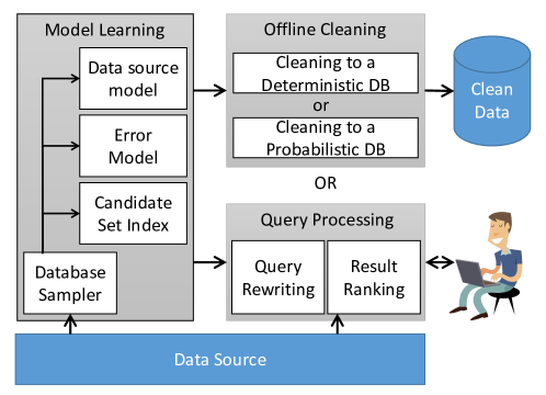
Figure 1: The architecture of BayesWipe. Our framework learns both data source model and error model from the raw data during the model learning phase. It can perform offline cleaning or query processing to provide clean data.

Figure 1 shows the system architecture for BayesWipe. During the model learning phase (Section 4), we first obtain a sample database by sending some queries to the database. On this sample data, we learn the generative model of the data as a Bayes network (Section 4.1). In parallel, we define and learn an error model which incorporates common kinds of errors (Section 4.2). We also create an index to quickly propose candidate $T^{*}$s.

We can then choose to do either offline cleaning (Section 5) or online query processing (Section 6), as per the scenario. In the offline cleaning mode, we iterate over all the tuples in the database and clean them one by one. We can choose whether to store the resulting cleaned tuple in a deterministic database (where we store only the $T^{*}$ with the maximum posterior probability) or probabilistic database (where we store the entire distribution over the $T^{*}$). In the online query processing mode, we obtain a query from the user, and do query rewriting in order to find a set of queries that are likely to retrieve a set of highly relevant tuples. We execute these queries and re-rank the results, and then display them.

Input: $D$, the dirty dataset.

$BN$ $\leftarrow$ Learn Bayes Network ($D$)

foreach Tuple $T\in D$ do

       $\mathcal{C}\leftarrow$ Find Candidate Replacements ($T$)

       foreach Candidate $T^{*}\in\mathcal{C}$ do

             $P(T^{*})\leftarrow$ Find Joint Probability ($T^{*},BN$)

             $P(T|T^{*})\leftarrow$ Error Model ($T,T^{*}$)

            

       end foreach

      $T\leftarrow\arg\displaystyle\max_{T^{*}\in\mathcal{C}}P(T^{*})P(T|T^{*})$

end foreach

Algorithm 1 The algorithm for offline data cleaning

Input: $D$, the dirty dataset

Input: $Q$, the user’s query

$S\leftarrow$ Sample the source dataset $D$

$BN$ $\leftarrow$ Learn Bayes Network ($S$)

$ES$ $\leftarrow$ Learn Error Statistics ($S$)

$R\leftarrow$ Query and score results ($Q,D,BN$)

$ESQ\leftarrow$ Get expanded queries ($Q$)

foreach Expanded query $E\in ESQ$ do

       $R\leftarrow R\,\cup$ Query and score results ($E,D,BN$)

       $RQ\leftarrow RQ\,\cup$ Get all relaxed queries ($E$)

      

end foreach

$Sort(RQ)$ by expected relevance, using $ES$

while top-$k$ confidence not attained do

       $B\leftarrow$ Pick and remove top $RQ$

       $R\leftarrow R\,\cup$ Query and score results ($B,D,BN$)

      

end while

$Sort(R)$ by score

return R

Algorithm 2 Algorithm for online query processing.

In Algorithms 1 and 2, we present the overall algorithm for BayesWipe. In the offline mode, we show how we iterate over all the tuples in the dirty database, $D$ and replace them with cleaned tuples. In the query processing mode, the first three operations are performed offline, and the remaining operations show how the tuples are efficiently retrieved from the database, ranked and displayed to the user.

4 Model Learning

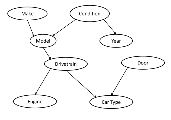
(a) Auto dataset

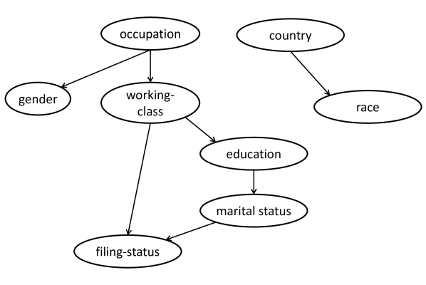
(b) Census dataset

Figure 2: The learned Bayes networks

This section details the process by which we estimate the components of Equation 2: the data source model ${\textbf{Pr}(T^{*})}$ and the error model ${\textbf{Pr}(T|T^{*})}$

4.1 Data Source Model

The data that we work with can have dependencies among various attributes (e.g., a car’s engine depends on its make). Therefore, we represent the data source model as a Bayes network, since it naturally captures relationships between the attributes via structure learning and infers probability distributions over values of the input tuples.

Constructing a Bayes network over ${\mathcal{D}}$ requires two steps: first, the induction of the graph structure of the network, which encodes the conditional independences between the $m$ attributes of ${\mathcal{D}}$’s schema; and second, the estimation of the parameters of the resulting network. The resulting model allows us to compute probability distributions over an arbitrary input tuple $T$.

Whenever the underlying patterns in the source database changes, we have to learn the structure and parameters of the Bayes network again. In our scenario, we observed that the structure of a Bayes network of a given dataset remains constant with small perturbations, but the parameters (CPTs) change more frequently. As a result, we spend a larger amount of time learning the structure of the network with a slower, but more accurate tool, Banjo [33]. Figures 2(a) and 2(b) show automatically learned structures for two data domains. The learned structure seems to be intuitively correct, since the nodes that are connected (for example, ‘country’ and ‘race’ in Figure 2(b)) are expected to be highly correlated.

Then, given a learned graphical structure ${\mathcal{G}}$ of ${\mathcal{D}}$, we can estimate the conditional probability tables (CPTs) that parameterize each node in ${\mathcal{G}}$ using a faster package called Infer.NET [35]. This process of inferring the parameters is run offline, but more frequently than the structure learning.

Once the Bayesian network is constructed, we can infer the joint distributions for arbitrary tuple $T$, which can be decomposed to the multiplication of several marginal distributions of the sets of random variables, conditioned on their parent nodes depending on ${\mathcal{G}}$.

4.2 Error Model

Having described the data source model, we now turn to the estimation of the error model ${\textbf{Pr}}(T|T^{*})$ from noisy data. There are many types of errors that can occur in data. We focus on the most common types of errors that occur in data that is manually entered by naïve users: typos, deletions, and substitution of one word with another. We also make an additional assumption that error in one attribute does not affect the errors in other attributes. This is a reasonable assumption to make, since we are allowing the data itself to have dependencies between attributes, while only constraining the error process to be independent across attributes. With these assumptions, we are able to come up with a simple and efficient error model, where we combine the three types of errors using a maximum entropy model.

Given a set of clean candidate tuples $\mathcal{C}$ where $T^{*}\in\mathcal{C}$, our error model ${\textbf{Pr}}(T|T^{*})$ essentially measures how clean $T$ is, or in other words, how similar $T$ is to $T^{*}$.

Edit distance similarity: This similarity measure is used to detect spelling errors. Edit distance between two strings $T_{A_{i}}$ and $T^{*}_{A_{i}}$ is defined as the minimum cost of edit operations applied to dirty tuple $T_{A_{i}}$ transform it to clean $T^{*}_{A_{i}}$. Edit operations include character-level copy, insert, delete and substitute. The cost for each operation can be modified as required; in this paper we use the Levenshtein distance, which uses a uniform cost function. This gives us a distance, which we then convert to a probability using [36]:

$$f_{ed}(T_{A_{i}},T_{A_{i}}^{*})=\exp\{-cost_{ed}(T_{A_{i}},T_{A_{i}}^{*})\}$$ (3)

Distributional Similarity Feature: This similarity measure is used to detect both substitution and omission errors. Looking at each attribute in isolation is not enough to fix these errors. We propose a context-based similarity measure called Distributional similarity ($f_{ds}$), which is based on the probability of replacing one value with another under a similar context [37]. Formally, for each string $T_{A_{i}}$ and $T_{A_{i}}^{*}$, we have:

$$f_{ds}(T_{A_{i}},T_{A_{i}}^{*})=\sum_{c\in C(T_{A_{i}},T_{A_{i}}^{*})}\frac{{\mathbf{Pr}}(c|T_{A_{i}}^{*}){\mathbf{Pr}}(c|T_{A_{i}}){\mathbf{Pr}}(T_{A_{i}})}{{\mathbf{Pr}}(c)}$$ (4)

where $C(T_{A_{i}},T_{A_{i}}^{*})$ is the context of a tuple attribute value, which is a set of attribute values that co-occur with both $T_{A_{i}}$ and $T_{A_{i}}^{*}$. ${\mathbf{Pr}}(c|T_{A_{i}}^{*})=(\#(c,T_{A_{i}}^{*})+\mu)/\#(T_{A_{i}}^{*})$ is the probability that a context value $c$ appears given the clean attribute $T_{A_{i}}^{*}$ in the sample database. Similarly, $P(T_{A_{i}})=\#(T_{A_{i}})/\#tuples$ is the probability that a dirty attribute value appears in the sample database. We calculate ${\mathbf{Pr}}(c|T_{A_{i}})$ and ${\mathbf{Pr}}(T_{A_{i}})$ in the same way. To avoid zero estimates for attribute values that do not appear in the database sample, we use Laplace smoothing factor $\mu$.

Unified error model: In practice, we do not know beforehand which kind of error has occurred for a particular attribute; we need a unified error model which can accommodate all three types of errors (and be flexible enough to accommodate more errors when necessary). For this purpose, we use the well-known maximum entropy framework [38] to leverage both the similarity measures, (Edit distance $f_{ed}$ and distributional similarity $f_{ds}$). For each attribute of the input tuple $T$ and $T^{*}$, we have the unified error model ${\mathbf{Pr}}(T|T^{*})$ given by:

$$\frac{1}{Z}\exp\left\{\alpha\sum_{i=1}^{m}f_{ed}(T_{A_{i}},T_{A_{i}}^{*})+\beta\sum_{i=1}^{m}f_{ds}(T_{A_{i}},T_{A_{i}}^{*})\right\}$$ (5)

where $\alpha$ and $\beta$ are the weight of each feature, $m$ is the number of attributes in the tuple. The normalization factor is $Z=\sum_{T^{*}}\exp\left\{\sum_{i}\lambda_{i}f_{i}(T^{*},T)\right\}$.

4.3 Finding the Candidate Set

The set of candidate tuples, $\mathcal{C}(T)$ for a given tuple $T$ are the possible replacement tuples that the system considers as possible corrections to $T$. The larger the set $\mathcal{C}$ is, the longer it will take for the system to perform the cleaning. If $\mathcal{C}$ contains many unclean tuples, then the system will waste time scoring tuples that are not clean to begin with.

An efficient approach to finding a reasonably clean $\mathcal{C}(T)$ is to consider the set of all the tuples in the sample database that differ from $T$ in not more than $j$ attributes. In order to find $\mathcal{C}(T)$ that satisfies this, conceptually, we have to iterate over every tuple $t$ in the sample database $D$, comparing it to the tuple $T$ and checking how many attributes it differs in. This operation can take $\mathcal{O}(n)$ time, where $n$ is the number of tuples in the sample database. Even with $j=3$, the naïve approach of constructing $\mathcal{C}$ from the sample database directly is too time consuming, since it requires one to go through the sample database in its entirety once for every result tuple encountered. To make this process faster, we create indices over $(j+1)$ attributes because searching through indices reduces the number of comparisons required to compute $\mathcal{C}(T)$. If any candidate tuple $T^{*}$ differs from $T$ in less than or equal to $j$ attributes, then it will be present in at least one of the indices, since we created $j+1$ of them (pigeon hole principle). These $j+1$ indices are created over those attributes that have the highest cardinalities, such as Make and Model (as opposed to attributes like Condition and Doors which can take only a few values). This ensures that the set of tuples returned from the index would be small in number.

For every possibly dirty tuple $T$ in the database, we go over each such index and find all the tuples that match the corresponding attribute. The union of all these tuples is then examined and the candidate set $\mathcal{C}$ is constructed by keeping only those tuples from this union set that do not differ from $T$ in more than $j$ attributes. Thus we can be sure that by using this method, we have obtained the entire set $\mathcal{C}$ .

5 Offline cleaning

5.1 Cleaning to a Deterministic Database

In order to clean the data in situ, we first use the techniques of the previous section to learn the data source model, the error model and create the index. Then, we iterate over all the tuples in the database and use Equation 1 to find the $T^{*}$ with the best score. We then replace the tuple with that $T^{*}$, thus creating a deterministic database using the offline mode of BayesWipe.

Computing ${\mathbf{Pr}}(T^{*}){\mathbf{Pr}}(T|T^{*})$ is very fast. Even though we do a Bayesian inference for ${\mathbf{Pr}}(T^{*})$, the tuple has all the values specified, so the inference ends up being a simple multiplication over the CPTs of the Bayes network, and is very cheap. ${\mathbf{Pr}}(T|T^{*})$ involves simple edit distance and distributional similarity calculations all of which involve simple arithmetic operations and lookups devoid of Bayesian inference.

Recall from Section 4.2 that there are parameters in the error model called $\alpha$ and $\beta$, which need to be set. Interestingly, in addition to controlling the relative weight given to the various features in the error model, these parameters can be used to control overcorrection by the system.

Overcorrection: Any data cleaning system is vulnerable to overcorrection, where a legitimate tuple is modified by the system to an unclean value. Overcorrection can have many causes. In a traditional, deterministic system, overcorrection can be caused by erroneous rules learned from infrequent data. For example, certain makes of cars are all owned by the same conglomerate (GM owns Chevrolet). In a misguided attempt to simplify their inventory, a car salesman might list all the cars under the name of the conglomerate. This may provide enough support to learn the wrong rule (Malibu $\to$ GM).

Typically, once an erroneous rule has been learned, there is no way to correct it or ignore it without a lot of oversight from domain experts. However, BayesWipe provides a way to regulate the amount of overcorrection in the system with the help of a ‘degree of change’ parameter. Without loss of generality, we can rewrite Equation 5 to the following:

$${\mathbf{Pr}}(T|T^{*}) =\frac{1}{Z}\exp\bigg{\{}\gamma\Big{(}\delta\sum_{i=1}^{m}f_{ed}(T_{A_{i}},T_{A_{i}}^{*})$$

$$\qquad\qquad+(1-\delta)\sum_{i=1}^{m}f_{ds}(T_{A_{i}},T_{A_{i}}^{*})\Big{)}\bigg{\}}$$

Since we are only interested in their relative weights, the parameters $\alpha$ and $\beta$ have been replaced by $\delta$ and $(1-\delta)$ with the help of a normalization constant, $\gamma$. This parameter, $\gamma$, can be used to modify the degree of variation in ${\mathbf{Pr}}(T|T^{*})$. High values of $\gamma$ imply that small differences in $T$ and $T^{*}$ cause a larger difference in the value of ${\mathbf{Pr}}(T|T^{*})$, causing the system to give higher scores to the original tuple (compared to a modified tuple).

Example: Consider the following fragment from the database. The first tuple is a very frequent tuple in the database, the second one is an erroneous tuple, and the third tuple is an infrequent, correct tuple. The ‘true’ correction of the second tuple is the third tuple. The ${\mathbf{Pr}}(T^{*})$ values shown reflect the values that the data source model might predict for them, roughly based on the frequency with which they occur in the source data.

Id	Make	Model	Type	Engine	Condition	$P(T^{*})$
1	Honda	Civic	Sedan	V4	New	0.400
2	Honda	Z4	Sedan	V6	New	0.001
3	BMW	Z4	Sedan	V6	New	0.005

A proper data cleaning system will correct tuple 2 to tuple 3, and not modify any of the others. However, if incorrect rules (for example, Z4 $\to$ Honda) were learned, there could be overcorrection, where tuple 3 is modified to tuple 2.

On the other hand, BayesWipe handles this situation based on the value of $\gamma$. Looking at tuple 3 (which is a clean tuple), suppose the candidate replacement tuples for it are also tuples 1, 2 and 3. In that case, the situation may look like the following:

		low $\gamma$		high $\gamma$
Cd.	$P(T^{*})$	$P(T|T^{*})$	score	$P(T|T^{*})$	score
1	0.400	0.02	0.0080	0.002	0.00080
2	0.001	0.30	0.0003	0.030	0.00003
3	0.005	1.00	0.0050	1.000	0.00500

As we can see, if we choose a low value of $\gamma$, the candidate with the highest score is tuple 1, which means an overcorrection will occur. However, with higher $\gamma$, the candidate with the highest score is tuple 3 itself, which means the tuple will not be modified, and overcorrection will not occur. On the other hand, if we set $\gamma$ too high, then even legitimately dirty tuples like tuple 2 won’t get changed, thus the number of actual corrections will also be lower.

To make full use of this capability of regulating overcorrection, we need to be able to set the value of $\gamma$ appropriately. In the absence of a training dataset (for which the ground truth is known), we can only estimate the best $\gamma$ approximately. We do this by finding a value of $\gamma$ for which the percentage of tuples modified by the system is equal to the expected percentage of noise in the dataset.

5.2 Cleaning to a Probabilistic Database

We note that many data cleaning approaches — including the one we described in the previous sections — come up with multiple alternatives for the clean version for any given tuple, and evaluate their confidence in each of the alternatives. For example, if a tuple is observed as ‘Honda, Corolla’, two correct alternatives for that tuple might be ‘Honda, Civic’ and ‘Toyota, Corolla’. In such cases, where the choice of the clean tuple is not an obvious one, picking the most-likely option may lead to the wrong answer. Additionally, if we intend to do further processing on the results, such as perform aggregate queries, join with other tables, or transfer the data to someone else for processing, then storing the most likely outcome is lossy.

A better approach (also suggested by others [4]) is to store all of the alternative clean tuples along with their confidence values. Doing this, however, means that the resulting database will be a probabilistic database (PDB), even when the source database is deterministic.

It is not clear upfront whether PDB-based cleaning will have advantages over cleaning to a deterministic database. On the positive side, using a PDB helps reduce loss of information arising from discarding all alternatives to tuples that did not have the maximum confidence. On the negative side, PDB-based cleaning increases the query processing cost (as querying PDBs are harder than querying deterministic databases [39]).

Another challenge is one of presentation: users usually assume that they are dealing with a deterministic source of data, and presenting all alternatives to them can be overwhelming to them. In this section, and in the associated experiments, we investigate the potential advantages to using the BayesWipe system and storing the resulting cleaned data in a probabilistic database. For our experiments, we used Mystiq [40], a prototype probabilistic database system from University of Washington, as the substrate. In order to create a probabilistic database from the corrections of the input data, we follow the offline cleaning procedure described previously in Section 4. Instead of storing the most likely $T^{*}$, we store all the $T^{*}$s along with their $P(T^{*}|T)$ values. When evaluating the performance of the probabilistic database, we used simple select queries on the resulting database. Since representing the results of a probabilistic database to the user is a complex task, in this paper we focus on showing the XOR representation of the tuple alternatives to the user. The rationale for our decision is that in a used car scenario, the user will be provided with a URL link to the car through the clickable tuple id and the several alternative clean values for the dirty attributes are shown within the single tuple returned to the user. As a result, the form of our output is a tuple-disjoint independent database [41]. This can be better explained with an example:

TABLE II: Cleaned probabilistic database

TID	Model	Make	Orig.	Size	Eng.	Cond.	P
$t_{1}$	Civic	Honda	JPN	Mid-size	V4	NEW	0.6
	Civic	Honda	JPN	Compact	V6	NEW	0.4
…
$t_{3}$	Civic	Honda	JPN	Mid-size	V4	USED	0.9
	Civik	Honda	JPN	Mid-size	V4	USED	0.1

Example: Suppose we clean our running example of Table I. We will obtain a tuple-disjoint independent probabilistic database [41]; a fragment of which is shown in Table II. Each original input tuple ($t_{1},t_{3}$), has been cleaned, and their alternatives are stored along with the computed confidence values for the alternatives (0.6 and 0.4 for $t_{1}$, in this example). Suppose the user issues a query Model = Civic. Both options of tuple $t_{1}$ of the probabilistic database satisfy the constraints of the query. Since there are two valid alternatives to tuple $t_{1}$ in the result with probabilities $0.6$ and $0.4$, in order to get a single tuple representation, the matching attributes in the alternatives are shown deterministically whereas the unclean attributes like Size, Engine and Condition with several possible clean values are shown as options. Only the first option in tuple $t_{3}$ matches the query. Thus the XOR result will contain only a single alternative for $t_{3}$ with probability 0.9. It is important to note that in the case of $t_{1}$, the Mid-size car can be associated with an Eng. value of V4 and a probability of 0.6 respectively. The XOR representation doesn’t necessarily allow for combining Mid-size with either an Eng. value of V6 or a probability value of 0.4.

The experimental results compare the tuple ids when computing the recall of the method because tuple id provides the URL to the car’s web page which can be used to determine a match. The output probabilistic relation is shown in Table III.

TABLE III: Result probabilistic database

TID	Model	Make	Orig.	Size	Eng.	Cond.	P
$t_{1}$	Civic	Honda	JPN	Mid-size/Compact	V4/V6	NEW	0.6/0.4
$t_{3}$	Civic	Honda	JPN	Mid-size	V4	USED	0.9

The interesting fact here is that the result of any query will always be a tuple-independent database. This is because we projected out every attribute except for the tuple-ID, and the tuple-IDs are independent of each other.

When showing the results of our experiments, we evaluate the precision and recall of the system. Since precision and recall are deterministic concepts, we have to convert the probabilistic database into a deterministic database (that will be shown to the user) prior to computing these values. We can do this conversion in two ways: (1) by picking only those tuples whose probability is higher than some threshold. We call this method the threshold based determinization. (2) by picking the top-$k$ tuples and discarding the probability values (top-$k$ determinization). The experiment section (Section 8.2) shows results with both determinizations.

6 Query rewriting for Online Query Processing

In this section we extend the techniques of the previous section so that it can be used in an online query processing method where the result tuples are cleaned at query time. Certain tuples that do not satisfy the query constraints, but are relevant to the user, need to be retrieved, ranked and shown to the user. The process also needs to be efficient, since the time that the users are willing to wait before results are shown to them is very small. We show our query rewriting mechanisms aimed at addressing both.

We begin by executing the user’s query ($Q^{*}$) on the database. We store the retrieved results, but do not show them to the user immediately. We then find rewritten queries that are most likely to retrieve clean tuples. We do that in a two-stage process: we first expand the query to increase the precision, and then relax the query by deleting some constraints (to increase the recall).

6.1 Increasing the precision of rewritten queries

We can improve precision by adding relevant constraints to the query $Q^{*}$ given by the user. For example, when a user issues the query Model = Civic, we can expand the query to add relevant constraints Make = Honda, Country = Japan, Size = Mid-Size. These additions capture the essence of the query — because they limit the results to the specific kind of car the user is probably looking for. These expanded structured queries generated from the user’s query are called $ESQ$s.

Each user query $Q^{*}$ is a select query with one or more attribute-value pairs as constraints. In order to create an $ESQ$, we will have to add highly correlated constraints to $Q^{*}$.

Searching for correlated constraints to add requires Bayesian inference, which is an expensive operation. Therefore, when searching for constraints to add to $Q^{*}$, we restrict the search to the union of all the attributes in the Markov blanket [42]. The Markov blanket of an attribute comprises its children, its parents, and its children’s other parents. It is the set of attributes whose value being given, the node becomes independent of all other nodes in the network. Thus, it makes sense to consider these nodes when finding correlated attributes. This correlation is computed using the Bayes Network that was learned offline on a sample database (recall the architecture of BayesWipe in Figure 1.)

Given a $Q^{*}$, we attempt to generate multiple $ESQ$s that maximizes both the relevance of the results and the coverage of the queries of the solution space.

Note that if there are $m$ attributes, each of which can take $n$ values, then the total number of possible $ESQ$s is $n^{m}$. Searching for the $ESQ$ that globally maximizes the objectives in this space is infeasible; we therefore approximately search for it by performing a heuristic-informed search. Our objective is to create an $ESQ$ with $m$ attribute-value pairs as constraints.We begin with the constraints specified by the user query $Q^{*}$. We set these as evidence in the Bayes network, and then query the Markov blanket of these attributes for the attribute-value pairs with the highest posterior probability given this evidence. We take the top-$k$ attribute-value pairs and append them to $Q^{*}$ to produce $k$ search nodes, each search node being a query fragment. If $Q$ has $p$ constraints in it, then the heuristic value of $Q$ is given by ${\textbf{Pr}}(Q)^{m/p}$. This represents the expected joint probability of $Q$ when expanded to $m$ attributes, assuming that all the constraints will have the same average posterior probability. We expand them further, until we find $k$ queries of size $m$ with the highest probabilities.

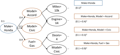
Figure 3: Query Expansion Example. The tree shows the candidate constraints that can be added to a query, and the rectangles show the expanded queries with the computed probability values.

Example: In Figure 3, we show an example of the query expansion. The node on the left represents the query given by the user “Make=Honda”. First, we look at the Markov Blanket of the attribute Make, and determine that Model and Condition are the nodes in the Markov blanket. we then set “Make=Honda” as evidence in the Bayes network and then run an inference over the values of the attribute Model. The two values of the Model attribute with the highest posterior probability are Accord and Civic. The most probable values of the Condition attribute are “new” and “old”. Using each of these values, new queries are constructed and added to the queue. Thus, the queue now consists of the 4 queries: “Make=Honda, Model=Civic”, “Make=Honda, Model=Accord” and “Make=Honda, Condition=old”. A fragment of these queries are shown in the middle column of Figure 3. We dequeue the highest probability item from the queue and repeat the process of setting the evidence, finding the Markov Blanket, and running the inference. We stop when we get the required number of $ESQ$s with a sufficient number of constraints.

6.2 Increasing the recall

Adding constraints to the query causes the precision of the results to increase, but reduces the recall drastically. Therefore, in this stage, we choose to delete some constraints from the $ESQ$s, thus generating relaxed queries ($RQ$). Notice that tuples that have corruptions in the attribute constrained by the user can only be retrieved by relaxed queries that do not specify a value for those attributes. Instead, we have to depend on rewritten queries that contain correlated values in other attributes to retrieve these tuples. Using relaxed queries can be seen as a trade-off between the recall of the resultset and the time taken, since there are an exponential number of relaxed queries for any given $ESQ$. As a result, an important question is the choice of $RQ$s to execute. We take the approach of generating every possible $RQ$, and then ranking them according to their expected relevance. This operation is performed entirely on the learned error statistics, and is thus very fast.

We score each relaxed query by the expected relevance of its result set.

$$Rank(q)=\mathbb{E}\left(\frac{\sum_{T_{q}}\textit{Score}(T_{q}|Q^{*})}{|T_{q}|}\right)$$

where $T_{q}$ are the tuples returned by a query $q$, and $Q^{*}$ is the user’s query. Executing an $RQ$ with a higher rank will have a more beneficial result on the result set because it will bring in better quality result tuples. Estimating this quantity is difficult because we do not have complete information about the tuples that will be returned for any query $q$. The best we can do, therefore, is to approximate this quantity.

Let the relaxed query be $Q$, and the expanded query that it was relaxed from be $ESQ$. We wish to estimate ${\mathbb{E}}[P(T|T^{*})]$ where $T$ are the tuples returned by $Q$. Using the attribute-error independence assumption, we can rewrite that as $\prod_{i=0}^{m}\textbf{Pr}(T.A_{i}|T^{*}.A_{i})$, where $T.A_{i}$ is the value of the $i$-th attribute in T. Since $ESQ$ was obtained by expanding $Q^{*}$ using the Bayes network, it has values that can be considered clean for this evaluation. Now, we divide the $m$ attributes of the database into 3 classes: (1) The attribute is specified both in $ESQ$ and in $Q$. In this case, we set ${\textbf{Pr}}(T.A_{i}|T^{*}.A_{i})$ to 1, since $T.A_{i}=T^{*}.A_{i}$. (2) The attribute is specified in $ESQ$ but not in $Q$. In this case, we know what $T^{*}.A_{i}$ is, but not $T.A_{i}$. However, we can generate an average statistic of how often $T^{*}.A_{i}$ is erroneous by looking at our sample database. Therefore, in the offline learning stage, we precompute tables of error statistics for every $T^{*}$ that appears in our sample database, and use that value. (3) The attribute is not specified in either $ESQ$ or $Q$. In this case, we know neither the attribute value in $T$ nor in $T^{*}$. We, therefore, use the average error rate of the entire attribute as the value for ${\textbf{Pr}}(T.A_{i}|T^{*}.A_{i})$. This statistic is also precomputed during the learning phase. This product gives the expected rank of the tuples returned by $Q$.

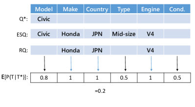
Figure 4: Query Relaxation Example.

Example: In Figure 4, we show an example for finding the probability values of a relaxed query. Assume that the user’s query $Q^{*}$ is “Civic”, and the $ESQ$ is shown in the second row. For an RQ that removes the attribute values “Civic” and “Mid-Size” from the $ESQ$, the probabilities are calculated as follows: For the attributes “Make, Country” and “Engine”, the values are present in both the $ESQ$ as well as the $RQ$, and therefore, the $P(T|T^{*})$ for them is 1. For the attribute “Model” and “Type”, the values are present in $ESQ$ but not in $RQ$, hence the value for them can be computed from the learned error statistics. For example, for “Civic”, the average value of $P(T|Civic)$ as learned from the sample database (0.8) is used. Finally, for the attribute “Condition”, which is present neither in $ESQ$ nor in $RQ$, we use the average error statistic for that attribute (i.e. the average of $P(T_{a}|T^{*}_{a})$ for $a$ = “Condition” which is 0.5).

The final value of ${\mathbb{E}}[P(T|T^{*})]$ is found from the product of all these attributes as 0.2. This process is very fast because it only involves lookups and multiplication - bayesian inference is not needed.

6.3 Terminating the process

We begin by looking at all the $RQ$s in descending order of their rank. If the current $k$-th tuple in our resultset has a relevance of $\lambda$, and the estimated rank of the $Q$ we are about to execute is $R(T_{q}|Q)$, then we stop evaluating any more queries if the probability ${\mathbf{Pr}}(R(T_{q}|Q)>\lambda)$ is less than some user defined threshold ${\mathcal{P}}$. This ensures that we have the true top-$k$ resultset with a probability ${\mathcal{P}}$.

7 Map-Reduce framework

BayesWipe is most useful for big-data related scenarios. BayesWipe has two modes: online and offline. The online mode of BayesWipe already works for big data scenarios by optimising the rewritten queries it issues. Now, we show that the offline mode can also be optimized for a big-data scenario by implementing it as a Map-Reduce application.

So far, BayesWipe-Offline has been implemented as a two-phase, single threaded program. In the first phase, the program learns the Bayes network (both structure and parameters), learns the error statistics, and creates the candidate index. Recall from section 4.3 that we create an index on the attributes of the sample database to speed up the creation of the candidate set of clean tuples; which we refer to as the candidate index. The candidate index is constructed on a set of $j+1$ attributes when the restriction on a candidate clean tuple is to differ from the dirty tuple in not more than $j$ attributes. The attributes in the dirty tuple are compared to the attributes of the tuples in the sample database using the candidate index to generate the set of candidate clean tuples. Note that this candidate index can be constructed on any arbitrary set of $j+1$ attributes present in the sample database. In the second phase, the program goes through every tuple in the input database, picks a set of candidate tuples, and then evaluates the $P(T^{*}|T)P(T^{*})$ for every candidate tuple, and replaces $T$ with the $T^{*}$ that maximises that value. Since the learning is typically done on a sample of the data, it is more important to focus on the second phase for the parallelizing efforts. Later, we will see how the learning of the error statistics can also be parallelized.

7.1 Simple Approach

The simplest approach to parallelizing BayesWipe is to run the first phase (the learning phase) on a single machine. Then, a copy of the bayes network (structure and CPTs), the error statistics, and the candidate index can be sent to a number of other machines. Each of those machines also receives a fraction of the input data from the dirty database. With the help of the generative model and the input data, it can clean the tuples, and then create the output.

If we express this in Map-Reduce terminology, we will have a pre-processing step where we create the generative and error models. The Map-Reduce architecture will have only mappers, and no reducers. The result of the mapping will be the tuple ${\langle T,T^{*}\rangle}$.

The problem with this approach is that in a truly big data scenario, the candidate index can become very large. Indeed, as the number of tuples increases, the size of the domain of each attribute also increases (see Figure 8(a) for 1 shard). Further, the number of different combinations, and the number of erroneous values for each attribute also increase (Figure 8(b)). All of this results in a rather large candidate index. Transmitting and using the entire index on each mapper node is wasteful of both network, memory, (and if swapped out, disk resources). Note that to create a rich and useful data correction system, we have to accommodate a large candidate clean-tuple set, ${\mathcal{C}}(T)$, for every $T$. ${\mathcal{C}}(T)$ roughly tracks the sample database size. If we are unable to shard ${\mathcal{C}}(T)$, then sharding the input data is pointless. In the following section we endeavor to show a strategy where not just the input, but also the index on the candidate set ${\mathcal{C}}(T)$ can be sharded across machines.

7.2 Improved Approach

In order to split both the input tuples and the candidate index, we use a two-stage approach. In the first stage, we run a map-reduce that splits the problem into multiple shards, each shard having a small fraction of the candidate index. The second stage is a simple map-reduce that picks the best output from stage 1 for each input tuple.

Stage 1: Given an input tuple $T$ and a set of candidate tuples, the $T^{*}$s, suppose the candidate index is created on $k$ attributes, $A_{1}...A_{k}$. We can say that for every tuple $T$, and one of its candidate tuples $T^{*}$, they will have at least one matching attribute $a_{i}$ from this set. We can use this common element $a_{i}$ to predict which shards the candidate $T^{*}$s might be available in. We therefore, send the tuple $T$ to each shard that matches the hash of the value $a_{i}$.

In the map-reduce architecture, it is possible to define a ‘partition’ function. Given a mapped key-value pair, this function determines which reducer nodes will process the data. We can use an exact equivalence on each value that the matching attribute can take, $a_{i}$ as the partition function. However, notice that the number of possible values that $A_{1}...A_{k}$ can take is rather large. If we naïvely use $a_{i}$ as the partition function, we will have to create those many reducer nodes. Therefore, more generally, we hash this value into a fixed number of reducer nodes, using a deterministic hash function. This will then find all candidate tuples that are eligible for this tuple, compute the similarity, and output it.

Example: Suppose we have tuple $T_{1}$ that has values $(a_{1},a_{2},a_{3},a_{4},a_{5})$. Suppose our candidate index is created on attributes $A_{1},A_{2},A_{4}$. This means that any candidates $T^{*}$ that are eligible for this tuple have to match one of the values $a_{1},a_{2}$ or $a_{4}$. Then the mapper will create the pairs $(a_{1},T)$, $(a_{2},T)$ and $(a_{4},T)$, and send to the reducers. The partition function is the hash of the key - so in this case, the first one will be sent to the reducer number $hash(A1=a1)$, the second will be sent to the reducer numbered $hash(A2=a2)$, and so on.

In the reducer, the similarity computation and computation of the prior probabilities from the BayesWipe algorithm are run. Since each reducer only has a fraction of the candidate index (the part that matches $A1=a1$, for instance), it can hold it in memory and computation is quite fast. Each reducer produces a pair $(T_{1},(T_{1n}^{*},{\text{score}}))$. Since there are several candidate clean tuples, $n$ is used to identify a specific tuple among those alternatives.

Stage 2: This stage is a simple $\max$ calculation. The mapper does nothing, it simply passes on the key-value pair $(T_{1},(T_{1n}^{*},{\text{score}}))$ that was generated in the previous Map-Reduce job. Notice that the key of this pair is the original, dirty tuple $T_{1}$. The Map-Reduce architecture thus automatically groups together all the possible clean versions of $T_{1}$ along with their scores. The reducer picks the best T* based on the score (using a simple $\max$ function), and outputs it to the database.

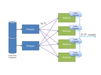
Figure 5: Stage-1 Map-Reduce Framework for BayesWipe.

7.3 Results of This Strategy

In Figure 8(a) and Figure 8(b) we can see how this map reduce strategy helps in reducing the memory footprint of the reducer. First, we plot the size of the index that needs to be held in each node as the number of tuples in the input increases. The topmost curve shows the size of index in bytes if there was no sharding - as expected, it increases sharply. The other curves show how the size of the index in the one of the nodes varies for the same dataset sizes. From the graph, it can be seen that as the number of tuples increases, the size of the index grows at a lower rate when the number of shards is increased. This shows that increasing the number of reduce nodes is a credible strategy for distributing the burden of the index.

In the second figure (Figure 8(b)), we see how the size of the index varies with the percentage of noise in the dataset. As expected, when the noise increases, the number of possible candidate tuples increase (since there are more variations of each attribute value in the pool). Without sharding, we see that the size of the dataset increases. While the increase in the size of the index is not as sharp as the increase due to the size of the dataset, it is still significant. Once again, we observe that as the number of shards is increased, the size of the index in the shard reduces to a much more manageable value.

Note that a slight downside to this architecture is that a shuffle/reduce of $(T,(T_{n}^{*},{\text{score}}))$ is needed in the second stage, and this intermediate data structure can be quite large. While this leads to some network and temporary storage overhead, the primary objective of sharding the expensive computation has been achieved by this architecture.

8 Empirical Evaluation

We quantitatively study the performance of BayesWipe in both its modes — offline, and online, and compare it against state-of-the-art CFD approaches. We present experiments on evaluating the approach in terms of the effectiveness of data cleaning, efficiency and precision of query rewriting. A demo for the offline cleaning mode of BayesWipe can be downloaded from http://bayeswipe.sushovan.de/.

8.1 Datasets

To perform the experiments, we obtained the real data from the web. The first dataset is Used car sales dataset $D_{car}$ crawled from Google Base. Such “dirty” dataset is referred to as “$D^{\prime}_{car}$”. The second dataset we used was adapted from the Census Income dataset $D_{census}$ from the UCI machine learning repository [43]. From the fourteen available attributes, we picked the attributes that were categorical in nature, resulting in the following 8 attributes: working-class, education, marital status, occupation, race, gender, filing status. country. The same setup was used for both datasets – including parameters and error features.

These datasets were observed to be mostly clean. We then introduced three types of noise to the attributes. To add noise to an attribute, we randomly changed it either to a new value which is close in terms of string edit distance (distance between 1 and 4, simulating spelling errors) or to a new value which was from the same attribute (simulating replacement errors) or just delete it (simulating deletion errors). As we have mentioned before, one of the assumptions of this paper is that the error model is a combination of these three kinds of errors, and that the errors are independent of each other. By synthetically generating these errors, we were able to test our system against a dataset that satisfies the assumption.

The next dataset tests our system against a real-world scenario where we do not control the error process, and thus validates that this assumption was not unrealistic.

To test our system against real-world noise where we do not have any control over amount, type or behavior of the noise generation process, we crawled car inventory data from the website ‘cars.com’. We manually verified that the data obtained did, in fact, have a reasonable number of inaccuracies, making it a suitable candidate for testing our system.

8.2 Experiments

Offline Cleaning Evaluation: The first set of evaluations shows the effectiveness of the offline cleaning mode. In Figure 6(a), we compare BayesWipe against CFDs [44].

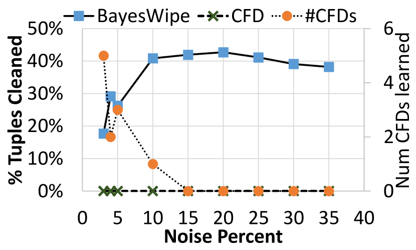
(a) % performance of BayesWipe compared to CFD, for the used-car dataset.

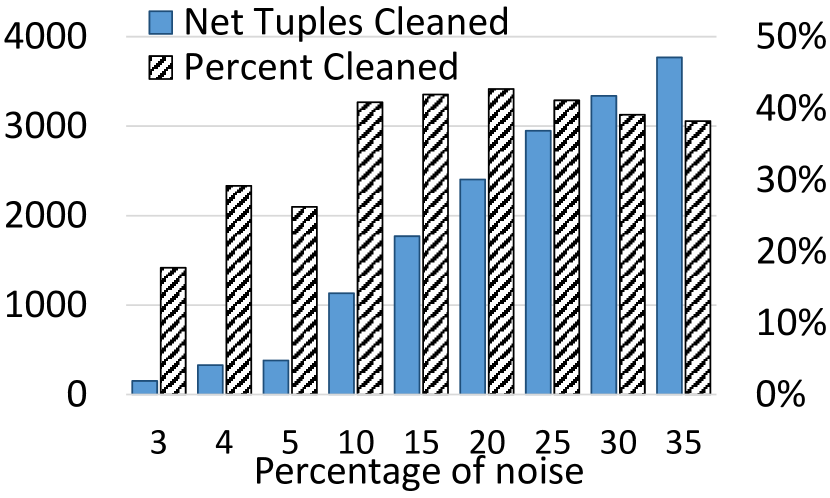
(b) % net corrupt values cleaned, car database

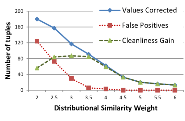
(c) Net corrections vs $\gamma$. (The $x$-axis values show the un-normalized distributional similarity weight, which is simply $\gamma\times 3/5$.)

Figure 6: Offline cleaning mode of BayesWipe

The dotted line that shows the number of CFDs learned from the noisy data quickly falls to zero, which is not surprising: CFDs learning was designed with a clean training dataset in mind. Further, the only constraints learned by this algorithm are the ones that have not been violated in the dataset — unless a tuple violates some CFD, it cannot be cleaned. As a result, the CFD method cleans exactly zero tuples independent of the noise percentage. On the other hand, BayesWipe is able to clean between 20% to 40% of the incorrect values. It is interesting to note that the percentage of tuples cleaned increases initially and then slowly decreases, because for very low values of noise, there aren’t enough errors for the system to learn a reliable error model from; and at larger values of noise, the data source model learned from the noisy data is of poorer quality.

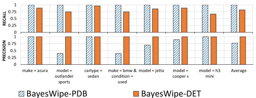
(a) Precision and recall of the PDB method shown against the deterministic method for specific queries.

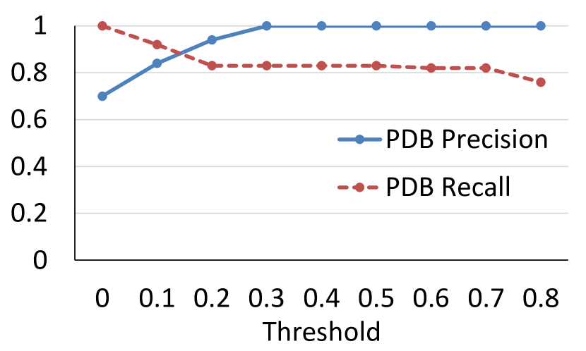
(b) Precision and recall of the PDB method using a threshold.

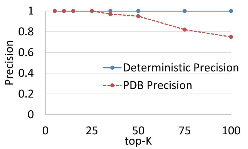
(c) top-$k$ precision of PDB vs deterministic method.

Figure 7: Results of probabilistic method.

While Figure 6(a) showed only percentages, in Figure 6(b) we report the actual number of tuples cleaned in the dataset along with the percentage cleaned. This curve shows that the raw number of tuples cleaned always increases with higher input noise percentages.

Setting $\gamma$: As explained in Section 5.1, the weight given to the edit distance ($\delta$) compared to the weight given to the distributional similarity ($1-\delta$); and the overcorrection parameter ($\gamma$) are parameters that can be tuned, and should be set based on which kind of error is more likely to occur. In our experiments, we performed a grid search to determine the best values of $\delta$ and $\gamma$ to use. In Figure 6(c), we show a portion of the grid search where $\delta=2/5$, and varying $\gamma$.

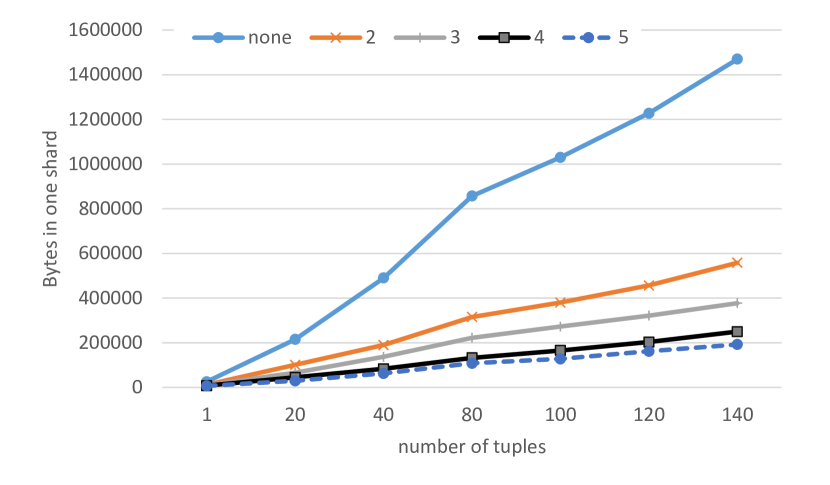
(a) vs the Number of Tuples (in Thousands) in the Dataset, for Various Number of Shards.

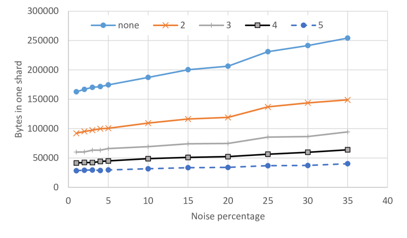
(b) vs the Noise in the Dataset, for Various Number of Shards.

Figure 8: Map-Reduce index sizes

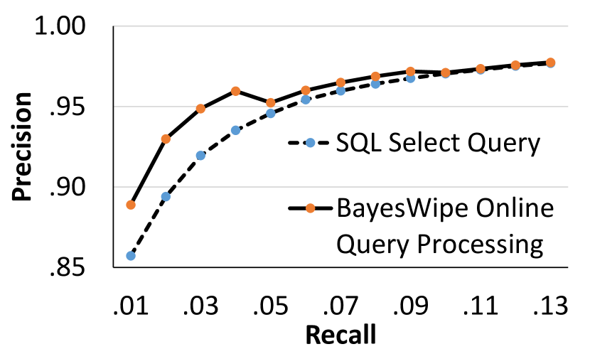
(c) Average precision vs recall

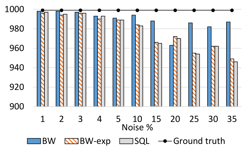
(d) Net improvement in data quality (TP-FP)

Figure 9: Online cleaning mode of BayesWipe

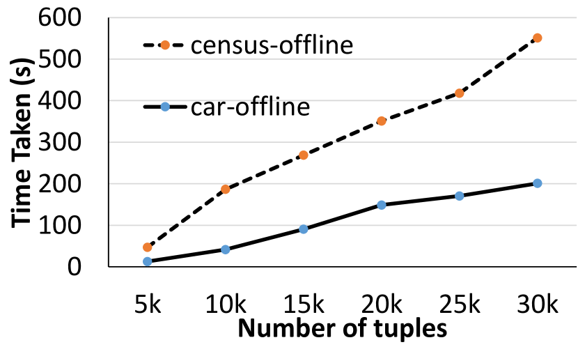
(a) Time taken vs number of tuples in offline mode

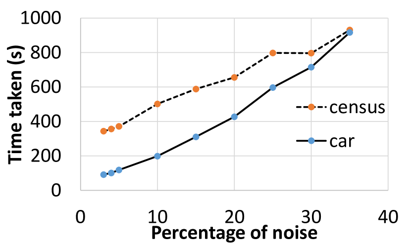
(b) Time taken vs noise percentage in offline mode

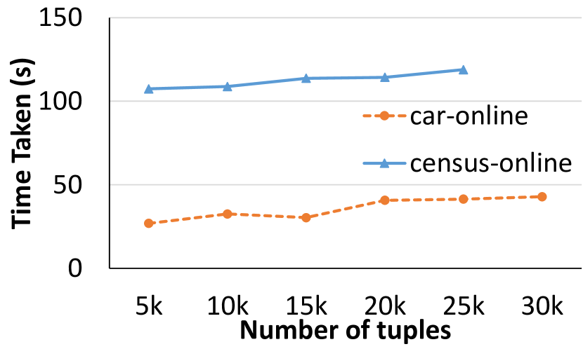
(c) Time taken vs number of tuples in online mode

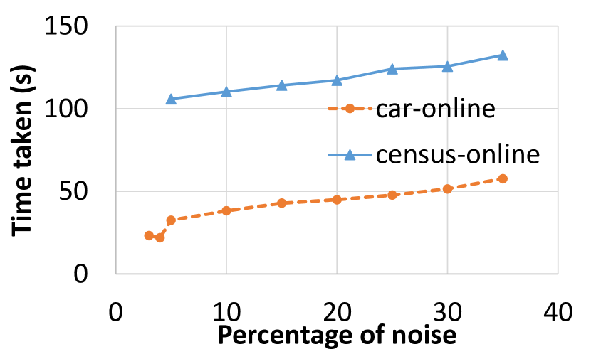
(d) Time taken vs noise percentage in online mode

Figure 10: Performance evaluations

The “values corrected” data points in the graph correspond to the number of erroneous attribute values that the algorithm successfully corrected (when checked against the ground truth). The “false positives” are the number of legitimate values that the algorithm changes to an erroneous value. When cleaning the data, our algorithm chooses a candidate tuple based on both the prior of the candidate as well as the likelihood of the correction given the evidence. Low values of $\gamma$ give a higher weight to the prior than the likelihood, allowing tuples to be changed more easily to candidates with high prior. The “overall gain” in the number of clean values is calculated as the difference of clean values between the output and input of the algorithm.

If we set the parameter values too low, we will correct most wrong tuples in the input dataset, but we will also ‘overcorrect’ a larger number of tuples. If the parameters are set too high, then the system will not correct many errors — but the number of ‘overcorrections’ will also be lower. Based on these experiments, we picked a parameter value of $\delta=0.638,\gamma=5.8$ and kept it constant throughout.

Using probabilistic databases: We empirically evaluate the PDB-mode of BayesWipe in Figure 7. In the first figure, we show the performance of the PDB mode of BayesWipe against the deterministic mode for specific queries. As we can see from the first, third and seventh queries, the BayesWipe-PDB improves the recall without any loss of precision. However, in most cases (and on average), BayesWipe-PDB provides a better recall at the cost of some precision.

The second figure shows the performance of BayesWipe-PDB as the probability threshold for inclusion of a tuple in the resultset is varied. As expected, with low values of the threshold, the system allows most tuples into the resultset, thus showing high recall and low precision. As the threshold increased, the precision increases, but the recall falls.

In Figure 7(c), we compare the precision of the PDB mode using top-$k$ determinization against the deterministic mode of BayesWipe. As expected, both the modes show high precision for low values of $k$, indicating that the initial results are clean and relevant to the user. For higher values of $k$, the PDB precision falls off, indicating that PDB methods are more useful for scenarios where high recall is important without sacrificing too much precision.

Online Query Processing: While in the offline mode, we had the luxury of changing the tuples in the database itself, in online query processing, we use query rewriting to obtain a resultset that is similar to the offline results, without modification to the database. We consider an SQL select query system as our baseline. We evaluate the precision and recall of our method against the ground truth and compare it with the baseline, using randomly generated queries.

We issued randomly generated queries to both BayesWipe and the baseline system. Figure 8(c) shows the average precision over 10 queries at various recall values. It shows that our system outperforms the SQL select query system in top-$k$ precision, especially since our system considers the relevance of the results when ranking them. On the other hand, the SQL search approach is oblivious to ranking and returns all tuples that satisfy the user query. Thus it may return irrelevant tuples early on, leading to less precision.

Figure 8(d) shows the improvement in the absolute numbers of tuples returned by the BayesWipe system. The graph shows the number of true positive tuples returned (tuples that match the query results from the ground truth) minus the number of false positives (tuples that are returned but do not appear in the ground truth result set). We also plot the number of true positive results from the ground truth, which is the theoretical maximum that any algorithm can achieve. The graph shows that the BayesWipe system outperforms the SQL query system at nearly every level of noise. Further, the graph also illustrates that — compared to an SQL query baseline — BayesWipe closes the gap to the maximum possible number of tuples to a large extent. In addition to showing the performance of BayesWipe against the SQL query baseline, we also show the performance of BayesWipe without the query relaxation part (called BW-exp). We can see that the full BayesWipe system outperforms the BW-exp system significantly, showing that query relaxation plays an important role in bringing relevant tuples to the resultset, especially for higher values of noise.

This shows that our proposed query ranking strategy indeed captures the expected relevance of the to-be-retrieved tuples, and the query rewriting module is able to generate the highly ranked queries.

Efficiency: In Figure 10 we show the data cleaning time taken by the system in its various modes. The first two graphs show the offline mode, and the second two show the online mode. As can be seen from the graphs, BayesWipe performs reasonably well both in datasets of large size and datasets with large noise.

Evaluation on real data with naturally occurring errors: In this section we used a dataset of 1.2 million tuples crawled from the cars.com website to check the performance of the system with real-world data, where the corruptions were not synthetically introduced. Since this data is large, and the noise is completely naturally occurring, we do not have ground truth for this data. To evaluate this system, we conducted an experiment on Amazon Mechanical Turk. First, we ran the offline mode of BayesWipe on the entire database. We then picked only those tuples that were changed during the cleaning, and then created an interface in mechanical turk where only those tuples were shown to the user in random order. Due to resource constraints, the experiment was run with the first 200 tuples that the system found to be unclean. We inserted 3 known answers into the questionnaire, and removed any responses that failed to annotate at least 2 out of the 3 answers correctly.

An example is shown in Figure 11. The turker is presented with two cars, and she does not know which of the cars was originally present in the dirty dataset, and which one was produced by BayesWipe. The turker will use her own domain knowledge, or perform a web search and discover that a Mazda CX-9 touring is only available in a 3.7l engine, not a 3.5l. Then the turker will be able to declare the second tuple as the correct option with high confidence.

The results of this experiment are shown in Table IV. As we can see, the users consistently picked the tuples cleaned by BayesWipe more favorably compared to the original dirty tuples, proving that it is indeed effective in real-world datasets. Notice that it is not trivial to obtain a 56% rate of success in these experiments. Finding a tuple which convinces the turkers that it is better than the original requires searching through a huge space of possible corrections. An algorithm that picks a possible correction randomly from this space is likely to get a near 0% accuracy.

The first row of Table IV shows the fraction of tuples for which the turkers picked the version cleaned by BayesWipe and indicated that they were either ‘very confident’ or ‘confident’. The second row shows the fraction of tuples for all turker confidence values, and therefore is a less reliable indicator of success.

In order to show the efficacy of BayesWipe we also performed an experiment in which the same tuples (the ones that BayesWipe had changed) were modified by a random perturbation. The random perturbation was done by the same error process as described before (typo, deletion, substitution with equal probability). Then these tuples (the original tuple from the database and the perturbed tuple) were presented as two choices to the turkers. The preference by the turkers for the randomly perturbed tuple over the original dirty tuple is shown in the third column, ‘Random’. It is obvious from this that the turkers overwhelmingly do not favor the random perturbed tuples. This demonstrates two things. First, it shows the fact that BayesWipe was performing useful cleaning of the tuples. In fact, BayesWipe shows a tenfold improvement over the random perturbation model, as judged by human turkers. This shows that in the large space of possible modifications of a wrong tuple, BayesWipe picks the correct one most of the time. Second, it provides additional support for the fact that the turkers are picking the tuple carefully, and are not randomly submitting their responses.

In this experiment, we also found the average fraction of known answers that the turkers gave wrong answers to. This value was 8%. This leads to the conclusion that the difference between the turker’s preference of BayesWipe over both the original tuples (which is 12%) and the random perturbation (which is 50%) are both significant.

Confidence	BayesWipe	Original	Random	Increase over Random
High confidence only	56.3%	43.6%	5.5%	50.8% points (10x better)
All confidence values	53.3%	46.7%	12.4%	40.9% points (4x better)

TABLE IV: Results of the Mechanical Turk Experiment, showing the percentage of tuples for which the users picked the results obtained by BayesWipe as against the original tuple. Also shows performance against a random modification.

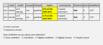
Figure 11: A fragment of the questionnaire provided to the Mechanical Turk workers.

9 Conclusion

In this paper we presented a novel system, BayesWipe that works using end-to-end probabilistic semantics, and without access to clean master data. We showed how to effectively learn the data source model as a Bayes network, and how to model the error as a mixture of error features. We showed the operation of this system in two modalities: (1) offline data cleaning, an in situ rectification of data and (2) online query processing mode, a highly efficient way to obtain clean query results over inconsistent data. There is an option to generate a standard, deterministic database as the output, as well as a probabilistic database, where all the alternatives are preserved for further processing. We empirically showed that BayesWipe outperformed existing baseline techniques in quality of results, and was highly efficient. We also showed the performance of the BayesWipe system at various stages of the query rewriting operation. We demonstrated how BayesWipe can be run on the map-reduce architecture so that it can scale to huge data sizes. User experiments showed that the system is useful in cleaning real-world noisy data.

Sushovan De is currently employed at Google. He graduated with a Ph.D. in Computer Science from Arizona State University. His research interests comprise Information Retrieval, Data Cleaning, and Probabilistic Databases.

Yuheng Hu is a Research Staff Member in the USER (User Systems and Experience Research) group at IBM Research - Almaden. He obtained his Ph.D in Computer Science at Arizona State University. His research interests are in the areas of Machine Learning, Social Computing and Human-Computer Interaction.

Meduri Venkata Vamsikrishna is a Ph.D student in Computer Science at Arizona State University. He received a Master’s degree in Computer Science from the National Unviersity of Singapore. His research interests include Data Mining from Social Media and Data Cleaning.

Yi Chen is an associate professor and the Henry J. Leir Chair in Healthcare in the School of Management with a joint appointment in the College of Computing Sciences at New Jersey Institute of Technology (NJIT). She received her Ph.D. degree in Computer Science from the University of Pennsylvania. Her current research focuses on Information Discovery on Big Data, Social Computing and Information Integration.

Subbarao Kambhampati is a professor in Computer Science at Arizona State University. He directs the Yochan research group which is associated with the Artifical Intelligence Lab at Arizona State University. He is the ”President-elect” of AAAI, the Association for the Advancement of Artificial Intelligence. He secured a Ph.D. degree in Computer Science from the University of Maryland, College Park. His research interests are Automated Planning in Artificial Intelligence and Data and Information Integration on the Web

References

- [1] W. Fan and F. Geerts, “Foundations of data quality management,” Synthesis Lectures on Data Management, 2012.
- [2] P. Gray, “Before Big Data, clean data,” 2013. [Online]. Available: http://www.techrepublic.com/blog/big-data-analytics/before-big-data-clean-data/
- [3] H. Leslie, “Health data quality – a two-edged sword,” 2010. [Online]. Available: http://omowizard.wordpress.com/2010/02/21/health-data-quality-a-two-edged-sword/
- [4] Computing Research Association, “Challenges and opportunities with big data,” http://cra.org/ccc/docs/init/bigdatawhitepaper.pdf, 2012.
- [5] E. Knorr, R. Ng, and V. Tucakov, “Distance-based outliers: algorithms and applications,” VLDB, 2000.
- [6] H. Xiong, G. Pandey, M. Steinbach, and V. Kumar, “Enhancing data analysis with noise removal,” TKDE, 2006.
- [7] P. Singla and P. Domingos, “Entity resolution with markov logic,” in ICDM, 2006.
- [8] I. Fellegi and D. Holt, “A systematic approach to automatic edit and imputation,” J. American Statistical association, 1976.
- [9] P. Bohannon, W. Fan, M. Flaster, and R. Rastogi, “A cost-based model and effective heuristic for repairing constraints by value modification,” in SIGMOD, 2005.
- [10] W. Fan, F. Geerts, L. Lakshmanan, and M. Xiong, “Discovering conditional functional dependencies,” ICDE, 2009.
- [11] L. E. Bertossi, S. Kolahi, and L. V. S. Lakshmanan, “Data cleaning and query answering with matching dependencies and matching functions,” ICDT, 2011.
- [12] A. Fuxman, E. Fazli, and R. J. Miller, “Conquer: Efficient management of inconsistent databases,” SIGMOD, 2005.
- [13] S. De, Y. Hu, Y. Chen, and S. Kambhampati, “Bayeswipe: A multimodal system for data cleaning and consistent query answering on structured bigdata,” IEEE Big Data, 2014.
- [14] G. Wolf, A. Kalavagattu, H. Khatri, R. Balakrishnan, B. Chokshi, J. Fan, Y. Chen, and S. Kambhampati, “Query processing over incomplete autonomous databases: query rewriting using learned data dependencies,” VLDB, 2009.
- [15] S. De, “Unsupervised bayesian data cleaning techniques for structured data,” Ph.D. dissertation, ASU, 2014.
- [16] P. Bohannon, W. Fan, F. Geerts, X. Jia, and A. Kementsietsidis, “Conditional functional dependencies for data cleaning,” ICDE, 2007.
- [17] W. Fan, F. Geerts, X. Jia, and A. Kementsietsidis, “Conditional functional dependencies for capturing data inconsistencies,” TODS, 2008.
- [18] J. Wang and N. Tang, “Towards dependable data repairing with fixing rules,”SIGMOD, 2014.
- [19] J. Wang, S. Krishnan, M. J. Franklin, K. Goldberg, T. Kraska, and T. Milo, “A sample-and-clean framework for fast and accurate query processing on dirty data,” SIGMOD, 2014.
- [20] L. Golab, H. J. Karloff, F. Korn, D. Srivastava, and B. Yu, “On generating near-optimal tableaux for conditional functional dependencies,” PVLDB, 2008.
- [21] G. Cormode, L. Golab, K. Flip, A. McGregor, D. Srivastava, and X. Zhang, “Estimating the confidence of conditional functional dependencies,” in SIGMOD, 2009.
- [22] M. Arenas, L. Bertossi, and J. Chomicki, “Consistent query answers in inconsistent databases,” PODS, 1999.
- [23] G. Cong, W. Fan, F. Geerts, X. Jia, and S. Ma, “Improving data quality: Consistency and accuracy,” VLDB, 2007.
- [24] M. Yakout, A. K. Elmagarmid, J. Neville, M. Ouzzani, and I. F. Ilyas, “Guided data repair,” VLDB, 2011.
- [25] G. Beskales, I. F. Ilyas, L. Golab, and A. Galiullin, “Sampling from repairs of conditional functional dependency violations,” VLDB, 2013.
- [26] W. Fan, J. Li, S. Ma, N. Tang, and W. Yu, “Towards certain fixes with editing rules and master data,” VLDB, 2010.
- [27] G. Beskales, I. F. Ilyas, L. Golab, and A. Galiullin, “On the relative trust between inconsistent data and inaccurate constraints,” ICDE, 2013.
- [28] X. L. Dong, L. Berti-Equille, and D. Srivastava, “Truth discovery and copying detection in a dynamic world,” VLDB,2009.
- [29] T. Dasu and J. M. Loh, “Statistical distortion: Consequences of data cleaning,” VLDB, 2012.
- [30] X. Chu, J. Morcos, I. F. Ilyas, M. Ouzzani, P. Papotti, N. Tang, and Y. Ye, “Katara: A data cleaning system powered by knowledge bases and crowdsourcing,” SIGMOD, 2015.
- [31] J. Wang, T. Kraska, M. J. Franklin, and J. Feng, “Crowder: Crowdsourcing entity resolution,” VLDB, 2012.
- [32] Y. Zheng, J. Wang, G. Li, R. Cheng, and J. Feng, “Qasca: A quality-aware task assignment system for crowdsourcing applications,” SIGMOD, 2015.
- [33] A. Hartemink., “Banjo: Bayesian network inference with java objects.” http://www.cs.duke.edu/~amink/software/banjo.
- [34] S. Russell and P. Norvig, Artificial intelligence: a modern approach. Prentice Hall, 2010.
- [35] T. Minka, W. J.M., J. Guiver, and D. Knowles, “Infer.NET 2.4”, Microsoft Research Cambridge, 2010. http://research.microsoft.com/infernet.
- [36] E. Ristad and P. Yianilos, “Learning string-edit distance,” Pattern Analysis and Machine Intelligence, IEEE Transactions on, 1998.
- [37] M. Li, Y. Zhang, M. Zhu, and M. Zhou, “Exploring distributional similarity based models for query spelling correction,” ICCL, 2006.
- [38] A. Berger, V. Pietra, and S. Pietra, “A maximum entropy approach to natural language processing,” Computational linguistics, 1996.
- [39] N. Dalvi and D. Suciu, “Efficient query evaluation on probabilistic databases,” VLDB, 2004.
- [40] J. Boulos, N. Dalvi, B. Mandhani, S. Mathur, C. Re, and D. Suciu, “Mystiq: a system for finding more answers by using probabilities,” SIGMOD, 2005.
- [41] D. Suciu and N. Dalvi, “Foundations of probabilistic answers to queries,” SIGMOD, 2005.
- [42] J. Pearl, Probabilistic Reasoning in Intelligent Systems: Networks of Plausible Inference. Morgan Kaufmann Publishers, 1988.
- [43] A. Asuncion and D. Newman, “UCI machine learning repository,” 2007.
- [44] F. Chiang and R. Miller, “Discovering data quality rules,” VLDB, 2008.