Stochastic Galerkin Methods for the Steady-State Navier-Stokes Equations

Abstract

We study the steady-state Navier-Stokes equations in the context of stochastic finite element discretizations. Specifically, we assume that the viscosity is a random field given in the form of a generalized polynomial chaos expansion. For the resulting stochastic problem, we formulate the model and linearization schemes using Picard and Newton iterations in the framework of the stochastic Galerkin method, and we explore properties of the resulting stochastic solutions. We also propose a preconditioner for solving the linear systems of equations arising at each step of the stochastic (Galerkin) nonlinear iteration and demonstrate its effectiveness for solving a set of benchmark problems.

1 Introduction

Models of mathematical physics are typically based on partial differential equations (PDEs) that use parameters as input data. In many situations, the values of parameters are not known precisely and are modeled as random fields, giving rise to stochastic partial differential equations. In this study we focus on models from fluid dynamics, in particular the stochastic Stokes and the Navier-Stokes equations. We consider the viscosity as a random field modeled as colored noise, and we use numerical methods based on spectral methods, specifically, the generalized polynomial chaos (gPC) framework [10, 14, 26, 27]. That is, the viscosity is given by a gPC expansion, and we seek gPC expansions of the velocity and pressure solutions.

There is a number of reasons to motivate our interest in Navier-Stokes equations with stochastic viscosity. For example, the exact value of viscosity may not be known, due to measurement error, the presence of contaminants with uncertain concentrations, or of multiple phases with uncertain ratios. Alternatively, the fluid properties might be influenced by an external field, with applications for example in magnetohydrodynamics. Specifically, we assume that the viscosity$~{}\nu$ depends on a set of random variables $\xi$. This means that the Reynolds number,

$$\operatorname{Re}\left(\xi\right)=\frac{UL}{\nu\left(\xi\right)},$$

where $U$ is the characteristic velocity and $L$ is the characteristic length, is also stochastic. Consequently, the solution variables are random fields, and different realizations of the viscosity give rise to realizations of the velocities and pressures. As observed in [19], there are other possible formulations and interpretations of fluid flow with stochastic Reynolds number for example, where the velocity is fixed but the volume of fluid moving into a channel is uncertain so the uncertainty derives from the Dirichlet inflow boundary condition.

We consider models of steady-state stochastic motion of an incompressible fluid moving in a domain $D\subset\mathbb{R}^{2}$. Extension to three-dimensional models is straightforward. We formulate the stochastic Stokes and Navier-Stokes equations using the stochastic finite element method, assuming that the viscosity has a general probability distribution parametrized by a gPC expansion. We describe linearization schemes based on Picard and Newton iteration for the stochastic Galerkin method, and we explore properties of the solutions obtained, including a comparison of the stochastic Galerkin solutions with those obtained using other approaches, such as Monte Carlo and stochastic collocation methods [26]. Finally, we propose efficient hierarchical preconditioners for iterative solution of the linear systems solved at each step of the nonlinear iteration in the context of the stochastic Galerkin method. Our approach is related to recent work by Powell and Silvester [19]. However, besides using a general parametrization of the viscosity, our formulation of the stochastic Galerkin system allows straightforward application of state-of-the-art deterministic preconditioners by wrapping them in the hierarchical preconditioner developed in [22]. For alternative preconditioners see, e.g., [2, 11, 17, 18, 20, 23, 25]. Finally, we note that there exist related approaches based on stochastic perturbation methods [13], important developments also include reduced-order models such as [4, 24], and an overview of existing methods for stochastic computational fluid dynamics can be found in the monograph [14].

The paper is organized as follows. In Section 2, we recall the deterministic steady-state Navier-Stokes equations and their discrete form. In Section 3, we formulate the model with stochastic viscosity, derive linearization schemes for the stochastic Galerkin formulation of the model, and explore properties of the resulting solutions for a set of benchmark problems that model the flow over an obstacle. In Section 4 we introduce a preconditioner for the stochastic Galerkin linear systems solved at each step of the nonlinear iteration, and in Section 5 we summarize our work.

2 Deterministic Navier-Stokes equations

We begin by defining the model and notation, following [6]. For the deterministic Navier-Stokes equations, we wish to find velocity$~{}\vec{u}$ and pressure$~{}p$ such that

$$-\nu\nabla^{2}\vec{u}+\left(\vec{u}\cdot\nabla\right)\vec{u}+\nabla p =\vec{f},$$ (1)

$$\nabla\cdot\vec{u} =0,$$ (2)

in a spatial domain$~{}D$, satisfying boundary conditions

$$\vec{u} =\vec{g},\quad\text{on }\Gamma_{\text{Dir}},$$ (3)

$$\nu\nabla\vec{u}\cdot\vec{n}-p\vec{n} =\vec{0},\quad\text{on }\Gamma_{\text{Neu}},$$ (4)

where$~{}\partial D=\overline{\Gamma}_{\text{Dir}}\cup\overline{\Gamma}_{\text{Neu}}$, and assuming sufficient regularity of the data. Dropping the convective term $\left(\vec{u}\cdot\nabla\right)\vec{u}$ from (1) yields the Stokes problem

$$-\nu\nabla^{2}\vec{u}+\nabla p =\vec{f},$$ (5)

$$\nabla\cdot\vec{u} =0.$$ (6)

The mixed variational formulation of (1)–(2) is to find $\left(\vec{u},p\right)\in\left(V_{E},Q_{D}\right)$ such that

$$\nu\int_{D}\nabla\vec{u}:\nabla\vec{v}+\int_{D}\left(\vec{u}\cdot\nabla\vec{u}\right)\vec{v}-\int_{D}p\left(\nabla\cdot\vec{v}\right) =\int_{D}\vec{f}\cdot\vec{v},\quad\forall\vec{v}\in V_{D},$$ (7)

$$\int_{D}q\left(\nabla\cdot\vec{u}\right) =0,\quad\forall q\in Q_{D},$$ (8)

where $\left(V_{D},Q_{D}\right)$ is a pair of spaces satisfying the inf-sup condition and $V_{E}$ is an extension of $V_{D}$ containing velocity vectors that satisfy the Dirichlet boundary conditions [3, 6, 12].

Let $c(\vec{z};\vec{u},\vec{v})\equiv\int_{\Omega}\left(\vec{z}\cdot\nabla\vec{u}\right)\cdot\vec{v}$. Because the problem (7)–(8) is nonlinear, it is solved using a linearization scheme in the form of Newton or Picard iteration, derived as follows. Consider the solution $\left(\vec{u},p\right)$ of (7)–(8) to be given as $\vec{u}=\vec{u}^{n}+\delta\vec{u}^{n}$ and $p=p^{n}+\delta p^{n}$. Substituting into (7)–(8) and neglecting the quadratic term $c(\delta\vec{u}^{n};\delta\vec{u}^{n},\vec{v})$ gives

$$\nu\int_{D}\nabla\delta\vec{u}^{n}:\nabla\vec{v}+c(\delta\vec{u}^{n};\vec{u}^{n},\vec{v})+c(\vec{u}^{n};\delta\vec{u}^{n},\vec{v})-\int_{D}\delta p^{n}\left(\nabla\cdot\vec{v}\right) =R^{n}\left(\vec{v}\right),$$ (9)

$$\int_{D}q\left(\nabla\cdot\delta\vec{u}^{n}\right) =r^{n}\left(q\right),$$ (10)

where

$$R^{n}\left(\vec{v}\right) =\int_{D}\vec{f}\cdot\vec{v}-\nu\int_{D}\nabla\vec{u}^{n}:\nabla\vec{v}-c(\vec{u}^{n};\vec{u}^{n},\vec{v})+\int_{D}p^{n}\left(\nabla\cdot\vec{v}\right),$$ (11)

$$r^{n}\left(q\right) =-\int_{D}q\left(\nabla\cdot\vec{u}^{n}\right).$$ (12)

Step $n$ of the Newton iteration obtains $\left(\delta\vec{u}^{n},\delta p^{n}\right)$ from (9)–(10) and updates the solution as

$$\vec{u}^{n+1} =\vec{u}^{n}+\delta\vec{u}^{n},$$ (13)

$$p^{n+1} =p^{n}+\delta p^{n}.$$ (14)

Step $n$ of the Picard iteration omits the term $c(\delta\vec{u}^{n};\vec{u}^{n},\vec{v})$ in (9), giving

$$\nu\int_{D}\nabla\delta\vec{u}^{n}:\nabla\vec{v}+c(\vec{u}^{n};\delta\vec{u}^{n},\vec{v})-\int_{D}\delta p^{n}\left(\nabla\cdot\vec{v}\right) =R^{n}\left(\vec{v}\right),$$ (15)

$$\int_{D}q\left(\nabla\cdot\delta\vec{u}^{n}\right) =r^{n}\left(q\right).$$ (16)

Consider the discretization of (1)–(2) by a div-stable mixed finite element method; for experiments discussed below, we used Taylor-Hood elements [6]. Let the bases for the velocity and pressure spaces be denoted $\left\{\phi_{i}\right\}_{i=1}^{N_{u}}$ and $\left\{\varphi_{i}\right\}_{i=1}^{N_{p}}$, respectively. In matrix terminology, each nonlinear iteration entails solving a linear system

$$\left[\begin{array}[c]{cc}\mathbf{F}^{n}&\mathbf{B}^{T}\\ \mathbf{B}&\mathbf{0}\end{array}\right]\left[\begin{array}[c]{c}\delta\mathbf{u}^{n}\\ \delta\mathbf{p}^{n}\end{array}\right]=\left[\begin{array}[c]{c}\mathbf{R}^{n}\\ \mathbf{r}^{n}\end{array}\right],$$ (17)

followed by an update of the solution

$$\mathbf{u}^{n+1} =\mathbf{u}^{n}+\delta\mathbf{u}^{n},$$ (18)

$$\mathbf{p}^{n+1} =\mathbf{p}^{n}+\delta\mathbf{p}^{n}.$$ (19)

For Newton’s method, $\mathbf{F}^{n}$ is the Jacobian matrix, a sum of the vector-Laplacian matrix $\mathbf{A}$, the vector-convection matrix $\mathbf{N}^{n}$, and the Newton derivative matrix $\mathbf{W}^{n}$,

$$\mathbf{F}^{n}=\mathbf{A}+\mathbf{N}^{n}+\mathbf{W}^{n},$$ (20)

where

$$\mathbf{A}\mathbf{=}\left[a_{ab}\right],\qquad a_{ab}=\nu\int_{D}\,\nabla\phi_{b}:\nabla\phi_{a}\mathbf{,}$$

$$\mathbf{N}^{n}=\left[n_{ab}^{n}\right],\qquad n_{ab}^{n}=\int_{D}\left(u^{n}\cdot\nabla\phi_{b}\right)\cdot\phi_{a},$$

$$\mathbf{W}^{n}=\left[w_{ab}^{n}\right],\qquad w_{ab}^{n}=\int_{D}\left(\phi_{b}\cdot\nabla u^{n}\right)\cdot\phi_{a}.$$

For Picard iteration, the Newton derivative matrix $\mathbf{W}^{n}$ is dropped, and $\mathbf{F}^{n}=\mathbf{A}+\mathbf{N}^{n}$. The divergence matrix $B$ is defined as

$$\mathbf{B}=\left[b_{cd}\right],\qquad b_{cd}=\int_{D}\phi_{d}\left(\nabla\cdot\varphi_{c}\right).$$ (21)

The residuals at step $n$ of both nonlinear iterations are computed as

$$\left[\begin{array}[c]{c}\mathbf{R}^{n}\\ \mathbf{r}^{n}\end{array}\right]=\left[\begin{array}[c]{c}\mathbf{f}\\ \mathbf{g}\end{array}\right]-\left[\begin{array}[c]{cc}\mathbf{P}^{n}&\mathbf{B}^{T}\\ \mathbf{B}&\mathbf{0}\end{array}\right]\left[\begin{array}[c]{c}\mathbf{u}^{n}\\ \mathbf{p}^{n}\end{array}\right],$$ (22)

where $\mathbf{P}^{n}=\mathbf{A}+\mathbf{N}^{n}$ and $\mathbf{f}$ is a discrete version of the forcing function of (1).

3 The Navier-Stokes equations with stochastic viscosity

Let $\left(\Omega,\mathcal{F},\mathcal{P}\right)$ represent a complete probability space, where $\Omega$ is the sample space, $\mathcal{F}$ is a$~{}\sigma$-algebra on $\Omega$ and $\mathcal{P}$ is a probability measure. We will assume that the randomness in the model is induced by a vector of independent, identically distributed (i.i.d.) random variables $\xi=\left(\xi_{1},\dots,\xi_{N}\right)^{T}$ such that $\xi:\Omega\rightarrow\Gamma\subset\mathbb{R}^{N}$. Let $\mathcal{F}_{\xi}\mathcal{\subset F}$ denote the $\sigma$-algebra generated by$~{}\xi$, and let $\mu\left(\xi\right)$ denote the joint probability density measure for $\xi$. The expected value of the product of random variables$~{}u$ and$~{}v$ that depend on$~{}\xi$ determines a Hilbert space $T_{\Gamma}\equiv L^{2}\left(\Omega,\mathcal{F}_{\xi},\mu\right)$ with inner product

$$\left\langle u,v\right\rangle=\mathbb{E}\left[uv\right]=\int_{\Gamma}u\left(\xi\right)v\left(\xi\right)\,d\mu\left(\xi\right),$$ (23)

where the symbol $\mathbb{E}$ denotes mathematical expectation.

3.1 The stochastic Galerkin formulation

The counterpart of the variational formulation (7)–(8) consists of performing a Galerkin projection on the space $T_{\Gamma}$ using mathematical expectation in the sense of (23). That is, we seek the velocity $\vec{u}$, a random field in $V_{E}\otimes T_{\Gamma}$, and the pressure $p\in Q_{D}\otimes T_{\Gamma}$, such that

$$\mathbb{E}\left[\int_{D}\!\nu\,\nabla\vec{u}:\nabla\vec{v}+\int_{D}\!\left(\vec{u}\cdot\nabla\vec{u}\right)\vec{v}-\int_{D}\!p\left(\nabla\cdot\vec{v}\right)\right] =\mathbb{E}\left[\int_{D}\!\vec{f}\cdot\vec{v}\right]\quad\forall\vec{v}\in V_{D}\otimes T_{\Gamma},$$ (24)

$$\mathbb{E}\left[\int_{D}\!q\left(\nabla\cdot\vec{u}\right)\right] =0\quad\forall q\in Q_{D}\otimes T_{\Gamma}.$$ (25)

The stochastic counterpart of the Newton iteration (9)–(10) is

$$\mathbb{E}\left[\int_{D}\nu\,\nabla\delta\vec{u}^{n}:\nabla\vec{v}+c(\vec{u}^{n};\delta\vec{u}^{n},\vec{v})+c(\delta\vec{u}^{n};\vec{u}^{n},\vec{v})-\int_{D}\delta p^{n}\left(\nabla\cdot\vec{v}\right)\right] =R^{n},$$ (26)

$$\mathbb{E}\left[\int_{D}q\left(\nabla\cdot\delta\vec{u}^{n}\right)\right] =r^{n},$$ (27)

where

$$R^{n}\left(\vec{v}\right) =\mathbb{E}\left[\int_{D}\vec{f}\cdot\vec{v}-\int_{D}\nu\,\nabla\vec{u}^{n}:\nabla\vec{v}-c(\vec{u}^{n};\vec{u}^{n},\vec{v})+\int_{D}p^{n}\left(\nabla\cdot\vec{v}\right)\right],$$ (28)

$$r^{n}\left(q\right) =-\mathbb{E}\left[\int_{D}q\left(\nabla\cdot\vec{u}^{n}\right)\right].$$ (29)

The analogue for Picard iteration omits $c(\delta\vec{u}^{n};\vec{u}^{n},\vec{v})$ from (26):

$$\mathbb{E}\left[\int_{D}\nu\,\nabla\delta\vec{u}^{n}:\nabla\vec{v}+c(\vec{u}^{n};\delta\vec{u}^{n},\vec{v})-\int_{D}\delta p^{n}\left(\nabla\cdot\vec{v}\right)\right]=R^{n}.$$ (30)

In computations, we will use a finite-dimensional subspace $T_{P}\subset T_{\Gamma}$ spanned by a set of polynomials $\left\{\psi_{\ell}\left(\xi\right)\right\}$ that are orthogonal with respect to the density function $\mu$, that is $\left\langle\psi_{k},\psi_{\ell}\right\rangle=\delta_{k\ell}$. This is referred to as the gPC basis; see [10, 27] for details and discussion. For $T_{P}$, we will use the space spanned by multivariate polynomials in $\{\xi_{j}\}_{j=1}^{N}$ of total degree $P$, which has dimension $M={\left(\!\!\begin{array}[c]{c}N+P\\ P\end{array}\!\!\right)}$. We will also assume that the viscosity is given by a gPC expansion

$$\nu=\sum_{\ell=0}^{M_{\nu}-1}\nu_{\ell}\left(x\right)\psi_{\ell}\left(\xi\right),$$ (31)

where $\left\{\nu_{\ell}\left(x\right)\right\}$ is a set of given deterministic spatial functions.

3.2 Stochastic Galerkin finite element formulation

We discretize (26) (or (30)) and (27) using div-stable finite elements as in Section 2 together with the gPC basis for $T_{P}$. For simplicity, we assume that the right-hand side $f\left(x\right)$ and the Dirichlet boundary conditions (3) are deterministic. This means in particular that, as in the deterministic case, the boundary conditions can be incorporated into right-hand side vectors (specified as $\mathbf{y}$ below). Thus, we seek a discrete approximation of the solution of the form

$$\vec{u}\left(x,\xi\right) \approx\sum_{k=0}^{M-1}\sum_{i=1}^{N_{u}}u_{ik}\phi_{i}(x)\psi_{k}(\xi)=\sum_{k=0}^{M-1}\vec{u}_{k}(x)\psi_{k}(\xi),$$ (32)

$$p\left(x,\xi\right) \approx\sum_{k=0}^{M-1}\sum_{j=1}^{N_{p}}p_{jk}\varphi_{j}(x)\psi_{k}(\xi)=\sum_{k=0}^{M-1}p_{k}(x)\psi_{k}(\xi),$$ (33)

The structure of the discrete operators depends on the ordering of the unknown coefficients $\{u_{ik}\}$, $\{p_{jk}\}$. We will group velocity-pressure pairs for each $k$, the index of stochastic basis functions (and order equations in the same way), giving the ordered list of coefficients

$$u_{1:N_{u},0},p_{1:N_{p},0},\,u_{1:N_{u},1},p_{1:N_{p},1},\,\ldots,\,u_{1:N_{u},M-1},p_{1:N_{p},M-1}.$$ (34)

To describe the discrete structure, we first consider the stochastic version of the Stokes problem (5)–(6), where the convection term $c(\cdot;\cdot,\cdot)$ is not present in (26) and (30). The discrete stochastic Stokes operator is built from the discrete components of the vector-Laplacian

$$\mathbf{A}_{\ell}\mathbf{=}\left[a_{\ell,ab}\right],\quad a_{\ell,ab}=\left(\int_{D}\nu_{\ell}\left(x\right)\,\nabla\phi_{b}:\nabla\phi_{a}\right),\qquad\ell=1,\ldots,M_{\nu}-1,$$ (35)

which are incorporated into the block matrices

$$\mathcal{S}_{0}=\left[\begin{array}[c]{cc}\mathbf{A}_{0}&\mathbf{B}^{T}\\ \mathbf{B}&\mathbf{0}\end{array}\right],\qquad\mathcal{S}_{\ell}=\left[\begin{array}[c]{cc}\mathbf{A}_{\ell}&\mathbf{0}\\ \mathbf{0}&\mathbf{0}\end{array}\right],\quad\ell=1,\dots,M_{\nu}-1.$$ (36)

These operators will be coupled with matrices arising from terms in $T_{P}$,

$$\mathbf{H}_{\ell}=\left[h_{\ell,jk}\right],\quad h_{\ell,jk}\equiv\mathbb{E}\left[\psi_{\ell}\psi_{j}\psi_{k}\right],\qquad\ell=0,\dots,M_{\nu}-1,\quad j,k=0,\dots,M-1.$$ (37)

Combining the expressions from (35), (36) and (37) and using the ordering (34) gives the discrete stochastic Stokes system

$$\left(\sum_{\ell=0}^{M_{\nu}-1}\mathbf{H}_{\ell}\otimes\mathcal{S}_{\ell}\right)\mathbf{v}=\mathbf{y},$$ (38)

where $\otimes$ corresponds to the matrix Kronecker product. The unknown vector $\mathbf{v}$ corresponds to the ordered list of coefficients in (34) and the right-hand side is ordered in an analogous way. Note that $\mathbf{H}_{0}$ is the identity matrix of order $M$.

Remark 1.

With this ordering, the coefficient matrix contains a set of $M$ block $2\times 2$ matrices of saddle-point structure along its block diagonal, given by

$$\mathcal{S}_{0}+\sum_{\ell=1}^{M_{\nu}-1}h_{\ell,jj}\mathcal{S}_{\ell},\qquad j=0,\ldots,M-1.$$

This enables the use of existing deterministic solvers for the individual diagonal blocks. An alternative ordering based on the blocking of all velocity coefficients followed by all pressure coefficients, considered in [19], produces a matrix of global saddle-point structure.

The matrices arising from the linearized stochastic Navier-Stokes equations augment the Stokes systems with stochastic variants of the vector-convection matrix and Newton derivative matrix appearing in (20). In particular, at step $n$ of the nonlinear iteration, let $\vec{u}_{\ell}^{n}(x)$ be the $\ell$th term of the velocity iterate (as in the expression on the right in (32) for $k=\ell$), and let

$$\mathbf{N}_{\ell}^{n}=\left[n_{\ell,ab}^{n}\right],\qquad n_{\ell,ab}^{n}=\int_{D}\left(\vec{u}_{\ell}^{n}\cdot\nabla\phi_{b}\right)\cdot\phi_{a},$$

$$\mathbf{W}_{\ell}^{n}=\left[w_{\ell,ab}^{n}\right],\qquad w_{\ell,ab}^{n}=\int_{D}\left(\phi_{b}\cdot\nabla\vec{u}_{\ell}^{n}\right)\cdot\phi_{a}.$$

Then the analogues of (35)–(36) are

$$\mathbf{F}_{\ell}^{n} =\mathbf{A}_{\ell}+\mathbf{N}_{\ell}^{n}+\mathbf{W_{\ell}}^{n},$$ for the stochastic Newton method (39)

$$\mathbf{F}_{\ell}^{n} =\mathbf{A}_{\ell}+\mathbf{N}_{\ell}^{n},$$ for stochastic Picard iteration, (40)

so for Newton’s method

$$\mathcal{F}_{0}^{n}=\left[\begin{array}[c]{cc}\mathbf{F}_{0}^{n}&\mathbf{B}^{T}\\ \mathbf{B}&\mathbf{0}\end{array}\right],\qquad\mathcal{F}_{\ell}^{n}=\left[\begin{array}[c]{cc}\mathbf{F}_{\ell}&\mathbf{0}\\ \mathbf{0}&\mathbf{0}\end{array}\right],$$ (41)

and as above, for Picard iteration the Newton derivative matrices $\{\mathbf{W}^{n}\}$ are dropped. Note that $\ell=0,\ldots,\widehat{M}-1$ here, where $\widehat{M}=\max\left(M,M_{\nu}\right)$. (In particular, if $M_{\nu}>M$, we set $\mathbf{N}_{\ell}^{n}=\mathbf{W}_{\ell}^{n}=0$ for $\ell=M+1,\dots,M_{\nu}-1$.) Step $n$ of the stochastic nonlinear iteration entails solving a linear system and updating,

$$\left[\sum_{\ell=0}^{\widehat{M}-1}\mathbf{H}_{\ell}\otimes\mathcal{F}_{\ell}^{n}\right]\delta\mathbf{v}^{n}=\mathcal{R}^{n},\qquad\mathbf{v}^{n+1}=\mathbf{v}^{n}+\delta\mathbf{v}^{n},$$ (42)

where

$$\mathcal{R}^{n}=\mathbf{y}-\left[\sum_{\ell=0}^{\widehat{M}-1}\mathbf{H}_{\ell}\otimes\mathcal{P}_{\ell}^{n}\right]\mathbf{v}^{n},$$ (43)

$\mathbf{v}^{n}$ and $\delta\mathbf{v}^{n}$ are vectors of current velocity and pressure coefficients and updates, respectively, ordered as in (34), $\mathbf{y}$ is the similarly ordered right-hand side determined from the forcing function and Dirichlet boundary data, and

$$\mathcal{P}_{0}^{n}=\left[\begin{array}[c]{cc}\mathbf{A}_{0}+\mathbf{N}_{0}^{n}&\mathbf{B}^{T}\\ \mathbf{B}&\mathbf{0}\end{array}\right],\qquad\mathcal{P}_{\ell}^{n}=\left[\begin{array}[c]{cc}\mathbf{A}_{\ell}+\mathbf{N}_{\ell}^{n}&\mathbf{0}\\ \mathbf{0}&\mathbf{0}\end{array}\right];$$

note that the $(1,1)$-blocks here are as in (40).

3.3 Sampling methods

In experiments described below, we compare some results obtained using stochastic Galerkin methods to those obtained from Monte Carlo and stochastic collocation. We briefly describe these approaches here.

Both Monte Carlo and stochastic collocation methods are based on sampling. This entails the solution of a number of mutually independent deterministic problems at a set of sample points $\left\{\xi^{\left(q\right)}\right\}$, which give realizations of the viscosity (31). That is, a realization of viscosity $\nu\left(\xi^{\left(q\right)}\right)$ gives rise to deterministic functions $\vec{u}\left(\cdot,\xi^{\left(q\right)}\right)$ and$~{}p\left(\cdot,\xi^{\left(q\right)}\right)$ on $D$ that satisfy the standard deterministic Navier-Stokes equations, and to finite-element approximations $\vec{u}^{(q)}(x)$, $p^{(q)}(x)$.

In the Monte Carlo method, the$~{}N_{MC}$ sample points are generated randomly, following the distribution of the random variables$~{}\xi$, and moments of the solution are obtained from ensemble averaging. For stochastic collocation, the sample points consist of a set of predetermined collocation points. This approach derives from a methodology for performing quadrature or interpolation in multidimensional space using a small number of points, a so-called sparse grid [8, 16]. There are two ways to implement stochastic collocation to obtain the coefficients in (32)–(33), either by constructing a Lagrange interpolating polynomial, or, in the so-called pseudospectral approach, by performing a discrete projection into $T_{P}$ [26]. We use the second approach because it facilitates a direct comparison with the stochastic Galerkin method. In particular, the coefficients are determined using a quadrature

$$u_{ik}=\sum_{q=1}^{N_{q}}\vec{u}^{(q)}\left(x_{i}\right)\,\psi_{k}\left(\xi^{\left(q\right)}\right)\,w^{\left(q\right)},\qquad p_{ik}=\sum_{q=1}^{N_{q}}p^{(q)}\left(x_{i}\right)\,\psi_{k}\left(\xi^{\left(q\right)}\right)\,w^{\left(q\right)},$$

where $\xi^{\left(q\right)}$ are collocation (quadrature) points, and $w^{\left(q\right)}$ are quadrature weights. We refer, e.g., to [14] for an overview and discussion of integration rules.

Fig. 1: Finite element mesh for the flow around an obstacle problem.

3.4 Example: flow around an obstacle

In this section, we present results of numerical experiments for a model problem given by a flow around an obstacle in a channel of length $12$ and height $2$. The viscosity (31) was taken to be a truncated lognormal process with mean values $\nu_{0}=1/50$ or $1/150$, which corresponds to mean Reynolds numbers $\operatorname{Re}_{0}=100$ or $300$, respectively, and its representation was computed from an underlying Gaussian random process using the transformation described in [9]. That is, for $\ell=0,\dots,M_{\nu}-1$, $\psi_{\ell}\left(\xi\right)$ is the product of $N$ univariate Hermite polynomials, and denoting the coefficients of the Karhunen-Loève expansion of the Gaussian process by $g_{j}\left(x\right)$ and $\eta_{j}=\xi_{j}-g_{j}$, $j=1,\dots,N$, the coefficients in the expansion (31) are computed as

$$\nu_{\ell}\left(x\right)=\mathbb{E}\left[\psi_{\ell}\left(\eta\right)\right]\exp\left[g_{0}\left(x\right)+\frac{1}{2}\sum_{j=1}^{N}\left(g_{j}\left(x\right)\right)^{2}\right].$$

The covariance function of the Gaussian field, for points $X_{1}=(x_{1},y_{1})$, $X_{2}=(x_{2},y_{2})\in D$, was chosen to be

$$C\left(X_{1},X_{2}\right)=\sigma_{g}^{2}\exp\left(-\frac{\left|x_{2}-x_{1}\right|}{L_{x}}-\frac{\left|y_{2}-y_{1}\right|}{L_{y}}\right),$$

where $L_{x}$ and $L_{y}$ are the correlation lengths of the random variables $\xi_{i}$, $i=1,\dots,N$, in the $x$ and $y$ directions, respectively, and $\sigma_{g}$ is the standard deviation of the Gaussian random field. The correlation lengths were set to be equal to $25\%$ of the width and height of the domain, i.e. $L_{x}=3$ and $L_{y}=0.5$. The coefficient of variation of the lognormal field, defined as $CoV=\sigma_{\nu}/\nu_{0}$ where $\sigma_{\nu}$ is the standard deviation, was $10\%$ or $30\%$. The stochastic dimension was $N=2$. The lognormal formulation was chosen to enable exploration of a general random field in which the viscosity guaranteed to be positive. See [1] for an example of the use of this formulation for diffusion problems and [28] for its use in models of porous media.

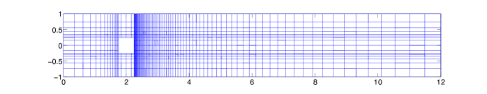
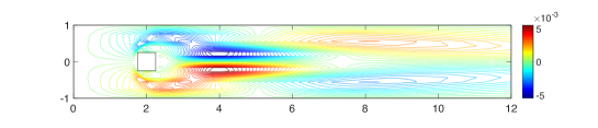
We implemented the methods in Matlab using IFISS 3.3 [5]. The spatial discretization uses a stretched grid, discretized by $1520$ Taylor-Hood finite elements; the domain and grid are shown in Figure 1. There are $12,640$ velocity and $1640$ pressure degrees of freedom. the degree used for the polynomial expansion of the solution was $P=3$, and the degree used for the expansion of the lognormal process was $2P$, which ensures a complete representation of the process in the discrete problem [15]. With these settings, $M=10$ and $M_{\nu}=\widehat{M}=28$, and $\mathbf{H}_{\ell}$ is of order $10$ in (42).

Fig. 2: Mean horizontal and vertical velocities and pressure (top) and variances of the same quantities (bottom), for $\operatorname{Re}=100$ and $CoV=10\%$.

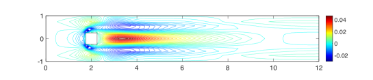
Consider first the case of $\operatorname{Re}_{0}=100$ and $CoV=10\%$. Figure 2 shows the mean horizontal and vertical components of the velocity and the mean pressure (top), and the variances of the same quantities (bottom). It can be seen that there is symmetry in all the quantities, the mean values are essentially the same as we would expect in the deterministic case, and the variance of the horizontal velocity component is concentrated in two “eddies” and is larger than the variance of the vertical velocity component. Figure 3 illustrates values of several coefficients of expansion (32) of the horizontal velocity. All the coefficients are symmetric, and as the index increases they become more oscillatory and their values decay. We found the same trends for the coefficients of the vertical velocity component and of the pressure. Our observations are qualitatively consistent with numerical experiments of Powell and Silvester [19].

Fig. 3: Coefficients $1-4$ of the gPC expansion of the horizontal velocity, $\operatorname{Re}_{0}=100$ and $CoV=10\%$.

Fig. 4: Variances of velocity components and pressure for $\operatorname{Re}_{0}=100$ and $CoV=30\%$.

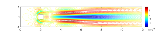
We also tested (the same) $\operatorname{Re}_{0}=100$ with increased $CoV=30\%$. We found that the mean values are essentially the same as in the previous case; Figure 4 shows the variances, which display the same qualitative behavior but have values that are approximately $10$ times larger than for the case $CoV=10\%$.

Fig. 5: Estimated pdfs of the velocities $u_{x}$ with $\operatorname{Re}_{0}=100$, $CoV=10\%$ (left) and $30\%$ (right) at the points with coordinates $(4.0100,-0.4339)$ (top) and $(4.0100,0.4339)$ (bottom).

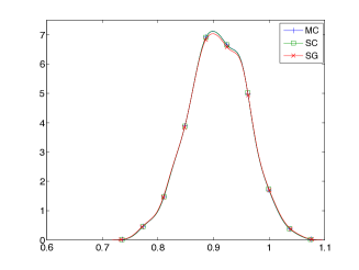
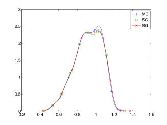
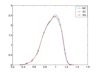
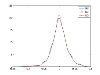
A different perspective on the results is given in Figure 5, which shows estimates of the probability density function (pdf) for the horizontal velocity at two points in the domain, $(4.0100,-0.4339)$ and $(4.0100,0.4339)$. These are locations at which large variances of the solution were seen, see Figures 2 and 4. The results were obtained using Matlab’s ksdensity function. It can be seen that with the larger value of $CoV$, the support of the velocity pdf is wider, and except for the peak values, for fixed $CoV$ the shapes of the pdfs at the two points are similar, indicating a possible symmetry of the stochastic solution. For this benchmark, we also obtained analogous data using the Monte Carlo and collocation sampling methods; it can be seen from the figure that these methods produced similar results.

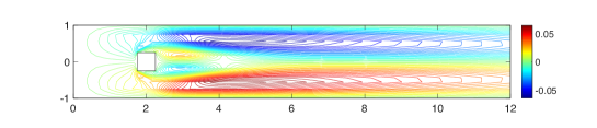
Next, we consider a larger value of the mean Reynolds number, $\operatorname{Re}_{0}=300$. Figure 6 shows the means and variances for the velocities and pressure for $CoV=10\%$. It is evident that increased $\operatorname{Re}_{0}$ results in increased values of the mean quantities, but they are again similar to what would be expected in the deterministic case. The variances exhibit wider eddies than for $\operatorname{Re}_{0}=100$, and in this case there is only one region of the largest variance in the horizontal velocity, located just to the right of the obstacle; this is also a region with increased variance of the pressure.

Fig. 6: Mean horizontal and vertical velocities and pressure (top) and variances of the same quantities (bottom), for $\operatorname{Re}_{0}=300$ and $CoV=10\%$.

In similar tests for the larger value $CoV=30\%$, we found that the mean values are essentially the same as for $CoV=10\%$, and Figure 7 shows the variances of velocities and pressures. From the figure it can be seen that the variances are qualitatively the same but approximately $10$ times larger than for $CoV=10\%$, results similar to those found for $\operatorname{Re}_{0}=100$.

Fig. 7: Variances of velocity components and pressure for $\operatorname{Re}_{0}=300$ and $CoV=30\%$.

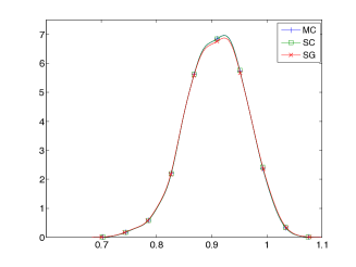
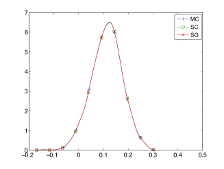
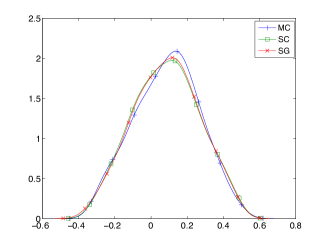
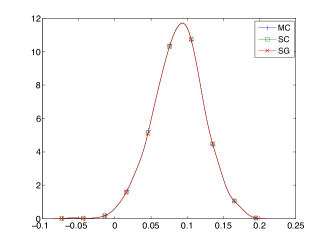
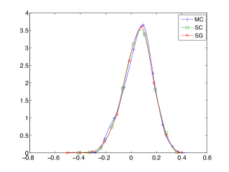
As above, we also examined estimated probability density functions for the velocities and pressures at a specified point in the domain, in this case, at the point $(3.6436,0)$, taken again from the region in which the solution has large variance. Figure 8 shows these pdf estimates, from which it can be seen that the three methods for handling uncertainty are in close agreement for each of the two values of $CoV$.

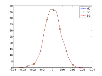
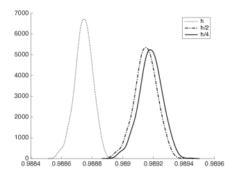
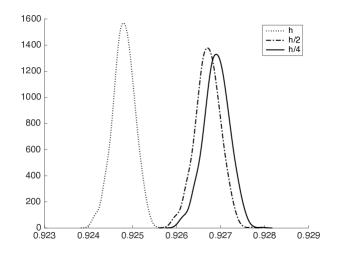
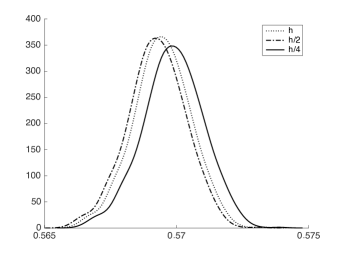
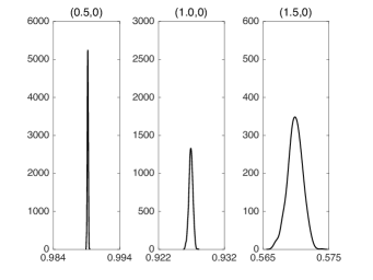
Finally, we show in Figure 9 the results of one additional experiment with $\operatorname{Re}_{0}=300$ and $CoV=10\%$, where estimated pdfs of the first velocity component $u_{x}$ were computed at three points near the inflow boundary, $(x,y)=(0.5,0)$, $(1,0)$ and $(1.5,0)$. These plots show some effects of spatial accuracy. The results for all methods were identical, and so only one representative pdf is shown. The images on the top and bottom left show results for a uniform mesh of width $h=1/8$ and for two refined meshes in which the horizontal mesh width to the left of the obstacle is reduced to $h/2$ and $h/4$. The image in the bottom right provides a more detailed view of the fine-grid results; in this image, the width of the horizontal window is the same ($0.01$) for the three subplots but the vertical heights are different. Several trends are evident:

• The pdfs at points nearer the boundary are much narrower.

• When the spatial accuracy is low, the methods miss some features of the pdf. In particular the methods produce a pdf that captures its “spiky” nature near the inflow, but the location of the spike is not correct.

We believe these effects stem from the fact that the inflow boundary is deterministic (with $u_{y}=1$ at $y=0$), and the effects of variability in the viscosity are felt less strongly at points near the inflow boundary. At points further from the deterministic inflow boundary, these effects and differences become less dramatic.

Fig. 8: Estimated pdfs of the velocities $u_{x}$ (top), $u_{y}$ (middle), and pressure$p$ (bottom) with $\operatorname{Re}_{0}=300$ and $CoV=10\%$ (left) and $30\%$ (right) at the point with coordinates $(3.6436,0)$.

Fig. 9: Estimated pdfs of the velocity $u_{x}$ at points $(0.5,0)$ (top left) $(1,0)$ (top right) and $(1.5,0)$ (bottom left), with $\operatorname{Re}_{0}=300$ and $CoV=10\%$ and three meshes. Bottom right: detailed depiction of the pdfs for each grid point obtained from the finest mesh.

3.5 Nonlinear solvers

We briefly comment on the nonlinear solution algorithm used to generate the results of the previous section. The nonlinear solver was implemented by modifying the analogue for deterministic systems in IFISS. It uses a hybrid strategy in which an initial approximation is obtained from solution of the stochastic Stokes problem (38), after which several steps of Picard iteration (equation (42) with $\mathcal{F}_{\ell}$ specified using (41) and (40)) are used to improve the solution, followed by Newton iteration ($\mathcal{F}_{\ell}$ from (39)). A convergent iteration stopped when the Euclidian norm of the algebraic residual (43) satisfied $\|\mathcal{R}^{n}\|_{2}\leq\epsilon\|y\|_{2}$ where $\epsilon=10^{-8}$ and $\mathbf{{y}}$ is as in (38).

In the experiments described in Section 3.4, we used values of the Reynolds number, $Re=100$ and $300$, and for each of these, two values of the coefficient of variation, $CoV=10\%$ and $30\%$. We list here the numbers of steps leading to convergence of the nonlinear algorithms that were used to generate the solutions discussed above. Direct solvers were used for the linear systems; we discuss a preconditioned iterative algorithm in Section 4 below.

$Re=100$,	$CoV=10\%$:	$6$ Picard steps	$1$ Newton step(s)
$Re=100$,	$CoV=30\%$:	6	2
$Re=300$,	$CoV=10\%$:	20	1
$Re=300$,	$CoV=30\%$:	20	2

Thus, a larger $CoV$ (larger standard deviation of the random field determining uncertainty in the process) leads to somewhat larger computational costs. For $Re=300$, the nonlinear iteration was not robust with $6$ initial Picard steps (for the stochastic Galerkin method as well as the sampling methods); $20$ steps was sufficient.

We also explored an inexact variant of these methods, in which the coefficient matrix of (42) for the Picard iteration was replaced by the block diagonal matrix $\mathbf{H}_{0}\otimes\mathcal{F}_{0}^{n}$ obtained from the mean coefficient. For $CoV=10\%$, with the same number of (now inexact) Picard steps as above ($6$ for $Re=100$ and $20$ for $Re=300$), this led to just one extra (exact) Newton step for $Re=100$ and no additional steps for $Re=300$. On the other hand, for $CoV=30\%$, this inexact method failed to converge.

4 Preconditioner for the linearized systems

The solution of the linear systems required during the course of the nonlinear iteration is a computationally intensive task, and use of direct solvers may be prohibitive for large problems. In this section, we present a preconditioning strategy for use with Krylov subspace methods to solve these systems, and we compare its performance with that of several other techniques. The new method is a variant of the hierarchical Gauss-Seidel preconditioner developed in [22].

4.1 Structure of the matrices and the preconditioner

We first recall the structure of the matrices $\{\mathbf{H}_{\ell}\}$ of (37). More comprehensive overviews of these matrices can be found in [7, 15]. The matrix structure can be understood through knowledge of the coefficient matrix $c_{P}\equiv\sum_{\ell=0}^{M_{\nu}-1}h_{\ell,jk}$ where $j,k=0,\dots,M-1$. The block sparsity structure depends on the type of coefficient expansion in (31). If only linear terms are included, that is $\psi_{\ell}=\xi_{\ell}$, $\ell=1,\dots,N$, then the coefficients $h_{\ell,jk}=\mathbb{E}\left[\xi_{\ell}\psi_{j}\psi_{k}\right]$ yield a Galerkin matrix with a block sparse structure. In the more general case, $h_{\ell,jk}=\mathbb{E}\left[\psi_{\ell}\psi_{j}\psi_{k}\right]$ and the stochastic Galerkin matrix becomes fully block dense. In either case, for fixed $\ell$ and a set of degree $\mathscr{P}$ polynomial expansions, with $1\leq\mathscr{P}\leq P$, the corresponding coefficient matrix $c_{\mathscr{P}}$ has a hierarchical structure

$$c_{\mathscr{P}}=\left[\begin{array}[c]{cc}c_{\mathscr{P}-1}&b_{\mathscr{P}}^{T}\\ b_{\mathscr{P}}&d_{\mathscr{P}}\end{array}\right],\qquad\mathscr{P}=1,\dots,P.$$

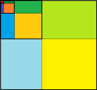
Now, let $\mathcal{A}_{P}$ denote the global stochastic Galerkin matrix corresponding to either a Stokes problem (38) or a linearized system (42); we will focus on the latter system in the discussion below. The matrix $\mathcal{A}_{P}$ also has a hierarchical structure

$$\mathcal{A}_{\mathscr{P}}=\left[\begin{array}[c]{cc}\mathcal{A}_{\mathscr{P}-1}&\mathcal{B}_{\mathscr{P}}\\ \mathcal{C}_{\mathscr{P}}&\mathcal{D}_{\mathscr{P}}\end{array}\right],\qquad\mathscr{P}=1,\dots,P,$$ (44)

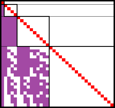
where $\mathcal{A}_{0}$ is the matrix of the mean, derived from $\nu_{0}$ in (31). This hierarchical structure is shown in the left side of Figure 10.

We will write vectors with respect to this hierarchy as

$$x_{\left(0:\mathscr{P}\right)}=\left[\begin{array}[c]{c}x_{\left(0\right)}\\ x_{\left(1\right)}\\ \vdots\\ x_{\left(\mathscr{P}\right)}\end{array}\right],$$

where $x_{\left(q\right)}$ includes all indices corresponding to polynomial degree $q$, blocked by spatial ordering determined by (34). With this notation, the global stochastic Galerkin linear system has the form

$$\mathcal{A}_{P}x_{\left(0:P\right)}=f_{\left(0:P\right)}.$$ (45)

To formulate the preconditioner for (45), we let $\widetilde{\mathcal{A}}_{0}$ represent an approximation of $\mathcal{A}_{0}$ and $\widetilde{\mathcal{D}}_{\mathscr{P}}$ represent an approximation of $\mathcal{D}_{\mathscr{P}}$. In particular, let

$$\widetilde{\mathcal{D}}_{\mathscr{P}}=\left[\begin{array}[c]{ccc}\widetilde{\mathcal{A}}_{0}&&\\ &\ddots&\\ &&\widetilde{\mathcal{A}}_{0}\end{array}\right],$$ (46)

where the number of diagonal blocks is given by $\mathscr{P}$. We will need the action of the inverse of $\widetilde{\mathcal{D}}_{\mathscr{P}}$, or an approximation to it, which can be obtained using an LU-factorization of $\widetilde{\mathcal{A}}_{0}$, or using some preconditioner for $\widetilde{\mathcal{A}}_{0}$, or using a Krylov subspace solver. A preconditioner $\mathcal{P}:w_{\left(0:\mathscr{P}\right)}\rightarrow v_{\left(0:\mathscr{P}\right)}$ for (45) is then defined as follows:

Algorithm 2.

[Approximate hierarchical Gauss-Seidel preconditioner (ahGS)] Solve (or solve approximately)

$$\widetilde{\mathcal{A}}_{0}v_{\left(0\right)}=w_{\left(0\right)},$$ (47)

and, for $\mathscr{P}$$=1,\ldots P$, solve (or solve approximately)

$$\widetilde{\mathcal{D}}_{\mathscr{P}}v_{\left(\mathscr{P}\right)}=\left(w_{\left(\mathscr{P}\right)}-\mathcal{C}_{\mathscr{P}}v_{\left(0:\mathscr{P}-1\right)}\right).$$ (48)

The cost of preconditioning can be reduced further by truncating the matrix-vector (MATVEC) operations used for the multiplications by the submatrices $\mathcal{C}_{\mathscr{P}}$ in (48). The idea is as follows. The system (45) can be written as

$$\sum_{j=0}^{M-1}\sum_{\ell=0}^{M_{\nu}-1}h_{\ell,jk}\mathcal{F}_{\ell}x_{j}=f_{k},\qquad k=0,\dots,M-1,$$ (49)

and the MATVEC with$~{}\mathcal{A}_{P}$ is given by

$$v_{j}=\sum_{k=0}^{M-1}\sum_{\ell=0}^{M_{\nu}-1}h_{\ell,jk}\mathcal{F}_{\ell}u_{k},$$ (50)

where the indices $j$, $k\in\left\{0,\dots,M-1\right\}$ correspond to nonzero blocks in$~{}\mathcal{A}_{P}$. The truncated MATVEC is an inexact evaluation of (50) proposed in [22, Algorithm 1], in which the summation over $\ell=0,\dots.M_{\nu}-1$ is replaced by summation over a subset $\mathcal{M}_{t}\subseteq\left\{0,\dots,M_{\nu}-1\right\}$. Figure 10 shows the hierarchical structure of the matrix and of the ahGS preconditioning operator. Both images in the figure correspond to the choice $P=3$, so that the hierarchical preconditioning operation (47)–(48) requires four steps. Because $N=4$, the matrix block size is $M=\left(\!\!\begin{array}[c]{c}N+P\\ P\end{array}\!\!\right)=35$. The block-lower-triangular component of the image on the right in Figure 10 shows the hierarchical structure of the ahGS preconditioning operator with truncation. For the matrix in the left panel, $M_{\nu}=\left(\!\!\begin{array}[c]{c}N+2P\\ 2P\end{array}\!\!\right)=210$, but the index set$~{}\mathcal{M}_{t}$ includes terms with indices at most $M-1$ in the accumulation of sums used for$~{}\mathcal{C}_{\mathcal{P}}$. These two heuristics, approximation by (46) and the truncation of MATVECs, significantly improve the sparsity structure of the preconditioner, on both the block diagonal (through the first technique) and the block lower triangle (through the second). In the next section, we will also consider truncated MATVECs with smaller maximal indices.

Fig. 10: Hierarchical structure of the stochastic Galerkin matrix (44) (left) and splitting operator $L+$diag$(D)$ for the approximate hierarchical Gauss-Seidel preconditioner (ahGS) with the truncation of the MATVEC (right).

4.2 Numerical experiments

In this section, we describe the results of experiments in which the ahGS preconditioner is used with GMRES to solve the systems arising from both Picard and Newton iteration. Unless otherwise specified, in the experiments discussed below, the block-diagonal matrices of (46), (47), (48) are taken to be $\widetilde{\mathcal{A}}_{0}=\mathcal{A}_{0}$, which corresponds to the first summand $\mathbf{H}_{0}\otimes\mathcal{F}_{0}^{n}$ in (42) and represents an approximation to the diagonal blocks of $\mathcal{D}_{\mathscr{P}}$; see also Remark 1. We also compare the performance of ahGS preconditioning with several alternatives:

• Mean-based preconditioner (MB) [17, 18], where the preconditioning operator is the block-diagonal matrix $\mathbf{H}_{0}\otimes\mathcal{F}_{0}^{n}=I\otimes\mathcal{F}_{0}^{n}$ derived from the mean of $\nu$.

• The Kronecker-product preconditioner [25] (denoted K), given by $\widehat{\mathbf{H}}_{0}\otimes\mathcal{F}_{0}^{n}$, where $\widehat{\mathbf{H}}_{0}$ is chosen to to minimize a measure of the difference $\mathcal{A}_{P}-\widehat{\mathbf{H}}_{0}\otimes\mathcal{F}_{0}^{n}$.

• Block Gauss-Seidel preconditioner (bGS), in which the preconditioning operation entails applying $(\widetilde{\mathcal{D}}_{\mathscr{P}}+L)^{-1}$ determined using the block lower triangle of $\mathcal{A}_{\mathcal{P}}$, that is with the approximation of the diagonal blocks by$~{}\mathcal{A}_{0}$ but without MATVEC truncation. This is an expensive operator but enables an understanding of the impact of various efforts to make the preconditioning operator more sparse.

• ahGS(PCD), a modification of ahGS in which the block-diagonal matrices of (47)–(48) are replaced by the pressure convection-diffusion (PCD) approximation [6] to the mean matrix $\mathcal{F}_{0}$ .

• ahGS(PCD-it), in which the block-diagonal solve of (48) is replaced by an approximate solve determined by twenty steps of a PCD-preconditioned GMRES iteration. For this strategy, $\widetilde{\mathcal{A}}_{0}$ in (47) and the blocks of $\widetilde{\mathcal{D}}_{\mathscr{P}}$ in (48) are taken to be the complete sum of (42), but the approximate solutions to these systems are obtained using a preconditioned inner iteration.

Four of the strategies, the ahGS, mean-based, Kronecker-product and bGS preconditioners, require the solution of a set of block-diagonal systems with the structure of a linearized Navier-Stokes operator of the form given in (17). We used direct methods for these computations. All results presented are for $\operatorname{Re}=100$; performance for $\operatorname{Re}=300$ were essentially the same. We believe this is because of the exact solves performed for the mean operators.

The results for the first step of Picard iteration are in Tables 1–4. All tests started with a zero initial iterate and stoppped when the residual $r^{(k)}=f_{(0:P)}-\mathcal{A}_{P}x_{(0:P)}^{(k)}$ for the $k$’th iterate satisfied $\|r^{(k)}\|_{2}\leq 10^{-8}\||f_{(0:P)}\|_{2}$ in the Euclidian norm. With other parameters fixed and no truncation of the MATVEC, Table 1 shows the dependence of GMRES iterations on the stochastic dimension $N$, Table 2 shows the dependence on the degree of polynomial expansion $P$, and Table 3 shows the dependence on the coefficient of variation $CoV$. It can be seen that the numbers of iterations with the ahGS preconditioner are essentially the same as with the block Gauss-Seidel (bGS) preconditioner, and they are much smaller compared to the mean-based (MB) and the Kronecker product preconditioners. When the exact solves with the mean matrix are replaced by the mean-based modified pressure-convection-diffusion (PCD) preconditioner for the diagonal block solves, the iterations grow rapidly. On the other hand, if the PCD preconditioner is used as part of an inner iteration as in ahGS(PCD-it), then good performance is recovered. This indicates that a good preconditioner for the mean matrix is an essential component of the global preconditioner for the stochastic Galerkin matrix.

Table 4 shows the iteration counts when the MATVEC operation is truncated in the action of the preconditioner. Truncation decreases the cost per iteration of the computation, and it can be also seen that performance can actually be improved. For example, with  $\ell_{t}=2$, the number of iterations is the smallest. Moreover there are only $21$ nonzeros in the lower triangular part of the sum of coefficient matrices $\{\mathbf{H}_{\ell}\}$ (each of which has order $10$) used in the MATVEC with $\ell_{t}\leq 2$, compared to $63$ nonzeros when no truncation is used; there are $203$ nonzeros in the set of $28$ full matrices $\{\mathbf{H}_{\ell}\}$.

Table 1: For Picard step: dependence on stochastic dimension $N$ of GMRES iteration counts, for various preconditioners, with polynomial degree $P=3$ and coefficient of variation $CoV=30\%$. $M$ is the block size of the stochastic Galerkin matrix, $M_{\nu}$ the number of terms in (31) and $ngdof$ the size of the stochastic Galerkin matrix.

$N$	$M$	$M_{\nu}$	$ngdof$	MB	K	bGS	ahGS	ahGS(PCD)	ahGS(PCD-it)
1	4	7	57,120	63	36	30	30	201	29
2	10	28	142,800	102	66	59	54	357	48
3	20	84	285,600	145	109	88	82	553	73

Table 2: For Picard step: dependence on polynomial degree $P$ of GMRES iteration counts, for various preconditioners, with stochastic dimension $N=3$ and coefficient of variation $CoV=30\%$. Other headings are as in Table 1.

$P$	$M$	$M_{\nu}$	$ngdof$	MB	K	bGS	ahGS	ahGS(PCD)	ahGS(PCD-it)
1	4	10	57,120	26	22	12	11	144	13
2	10	35	142,800	63	49	29	26	300	29
3	20	84	285,600	145	109	88	82	553	73

Table 3: For Picard step: dependence on coefficient of variation $CoV$ of GMRES iteration counts, for various preconditioners, with stochastic dimension $N=2$ and polynomial degree $P=3$. Other headings are as in Table 1.

$CoV(\%)$	MB	K	bGS	ahGS	ahGS(PCD)	ahGS(PCD-it)
10	16	14	7	7	186	10
20	36	27	17	16	259	17
30	102	66	59	54	357	48

Table 4: For Picard step: number of GMRES iterations when the preconditioners use truncated MATVEC. The matrices corresponding to higher degree expansion of the coefficient than $\ell_{t}$ are dropped from the action of the preconditioner. Here $N=2$, $P=3$, $M_{t}$ is the number of terms used in the inexact (truncated) evaluation of the MATVEC (50), $nnz(c_{\ell})$ is the number of nonzeros in the lower triangular parts of the coefficient matrices (37) after the truncation. Other headings are as in Table 1.

setup	$\ell_{t}$	0	1	2	3	6
	$M_{t}$	1	3	6	10	28
	$nnz(c_{\ell})$	0	12	21	43	63
bGS
CoV (%)	10	16	9	7	7	7
	20	36	19	15	17	17
	30	102	55	43	57	58
ahGS
CoV (%)	10	16	9	7	7	7
	20	36	19	14	16	16
	30	102	55	35	55	54

Results for the first step of Newton iteration, which comes after six steps of Picard iteration, are summarized in Tables 5–8. As above, the first three tables show the dependence on stochastic dimension $N$ (Table 5), polynomial degree $P$ (Table 6), and coefficient of variation $CoV$ (Table 7). It can be seen that all iteration counts are higher compared to corresponding results for the Picard iteration, but the other trends are very similar. In particular, the performances of the ahGS and bGS preconditioners are comparable except for the case when $N=3$, and $P=3$ (the last rows in Tables 5 and 6). Nevertheless, checking results in Table 8, which shows the effect of truncation, it can be seen that with the truncation of the MATVEC the iteration counts of the ahGS and bGS preconditioners can be further improved. Indeed, running one more experiment for the aforementioned case when $N=3$, and $P=3$, it turns out that with $\ell_{t}=2$ the number of iterations with the ahGS and bGS preconditioners are $118$ and $120$, respectively and with $\ell_{t}=3$ they are $101$ and $104$, respectively. That is, the truncation leads to fewer iterations also in this case, and the performance of ahGS and bGS preconditioners is again comparable.

Table 5: For Newton step: dependence on stochastic dimension $N$ of GMRES iteration counts, for various preconditioners, with polynomial degree $P=3$ and coefficient of variation $CoV=30\%$. Other headings are as in Table 1.

$N$	$M$	$M_{\nu}$	$ngdof$	MB	K	bGS	ahGS	ahGS(PCD)	ahGS(PCD-it)
1	4	7	57,120	73	42	32	32	309	40
2	10	28	142,800	126	80	77	69	546	63
3	20	84	285,600	235	170	128	151	1011	117

Table 6: For Newton step: dependence on polynomial degree $P$ of GMRES iteration counts, for various preconditioners, with stochastic dimension $N=3$ and coefficient of variation $CoV=30\%$. Other headings are as in Table 1.

$P$	$M$	$M_{\nu}$	$ngdof$	MB	K	bGS	ahGS	ahGS(PCD)	ahGS(PCD-it)
1	4	10	57,120	27	23	12	11	219	32
2	10	35	142,800	68	55	33	32	450	42
3	20	84	285,600	235	170	128	151	1011	117

Table 7: For Newton step: dependence on coefficient of variation $CoV$ of GMRES iteration counts, for various preconditioners, with stochastic dimension $N=2$ and polynomial degree $P=3$. Other headings are as in Table 1.

$CoV(\%)$	MB	K	bGS	ahGS	ahGS(PCD)	ahGS(PCD-it)
10	17	15	8	8	322	28
20	40	30	20	19	379	35
30	126	80	77	69	546	63

Table 8: For Newton step: number of GMRES iterations when the preconditioners use the truncation of the MATVEC. Headings are as in Table 4.

setup	$\ell_{t}$	0	1	2	3	6
	$M_{t}$	1	3	6	10	28
	$nnz(c_{\ell})$	0	12	21	43	63
bGS
CoV (%)	10	17	10	8	8	8
	20	40	22	18	20	20
	30	126	68	57	75	77
ahGS
CoV (%)	10	17	10	8	8	8
	20	40	22	17	19	19
	30	126	68	45	70	69

Finally, we briefly discuss computational costs. For any preconditioner, each GMRES step entails a matrix-vector product by the coefficient matrix. For viscosity given by a general probability distribution, this will typically involve a block-dense matrix, and, ignoring any overhead associated with increasing the number of GMRES steps, this will be the dominant cost per step. The mean-based preconditioner requires the action of the inverse of the block-diagonal matrix $I\otimes\mathcal{F}_{0}^{n}$. This has relatively small amount of overhead once the factors of $\mathcal{F}_{0}^{n}$ are computed. The ahGS preconditioner without truncation effectively entails a matrix-vector product by the block lower-triangular part of the coefficient matrix, so its overhead is bounded by $50\%$ of the cost of a multiplication by the coefficient matrix. This is an overestimate because it ignores the approximation of the block diagonal and the effect of truncation. For example, consider the case with stochastic dimension $N=2$ and polynomial expansions of degree $P=3$ for the solution and $2P=6$ for the viscosity; this gives $M=10$ and $M_{\nu}=28$. In Tables 4 and 8, $M_{t}$ indicates how many matrices are used in the MATVEC operations and $nnz(c_{\ell})$ is the number of nonzeros in the sum of the lower triangular parts of the coefficient matrices $\{\mathbf{H}_{\ell}\,|\,\ell=0,\ldots,M_{t}-1\}$. With complete truncation, $\ell_{t}=0$, and ahGS reduces to the mean-based preconditioner. With no truncation, $\ell_{t}=6$, and because the number of nonzeros in $\{\mathbf{H}_{\ell}\}$ is $203$, the overhead of ahGS is $63/203$, less than $30\%$ of the cost of multiplication by the coefficient matrix. If truncation is used, in particular when the iteration count is the lowest ($\ell_{t}=2$), the overhead is only $21/203\doteq 10\%$. Note that with increasing stochastic dimension and degree of polynomial expansion, the savings will be higher because the ratio of the sizes of the blocks $\mathcal{C}_{\mathscr{P}}/\mathcal{D}_{\mathscr{P}}$ decreases as $P$ increases, see (44). Last, the mean-based preconditioner is embarrassingly parallel; the ahGS preconditioner requires $P+1$ sequential steps, although each of these steps is also highly parallelizable. The Kronecker preconditioner is more difficult to assess because it does not have block-diagonal structure, and we do not discuss it here.

5 Conclusion

We studied the Navier-Stokes equations with stochastic viscosity given in terms of polynomial chaos expansion. We formulated the stochastic Galerkin method and proposed its numerical solution using a stochastic versions of Picard and Newton iteration, and we also compared its performance in terms of accuracy with that of stochastic collocation and Monte Carlo method. Finally, we presented a methodology of Gauss-Seidel hierarchical preconditioning with approximation using the mean-based diagonal block solves and a truncation of the MATVEC operations. The advantage of this approach is that neither the matrix nor the preconditioner need to be formed explicitly, and the ingredients include only the matrices from the polynomial chaos expansion and a good preconditioner for the mean-value deterministic problem, it allows an obvious parallel implementation, and it can be written as a “wrapper” around existing deterministic code.

References

- [1] I. Babuška, F. Nobile, and R. Tempone. A stochastic collocation method for elliptic partial differential equations with random input data. SIAM Journal on Numerical Analysis, 45:1005–1034, 2007.
- [2] M. Brezina, A. Doostan, T. Manteuffel, S. McCormick, and J. Ruge. Smoothed aggregation algebraic multigrid for stochastic PDE problems with layered materials. Numerical Linear Algebra with Applications, 21(2):239–255, 2014.
- [3] F. Brezzi and M. Fortin. Mixed and Hybrid Finite Element Methods. Springer-Verlag, New York – Berlin – Heidelberg, 1991.
- [4] H. C. Elman and Q. Liao. Reduced basis collocation methods for partial differential equations with random coefficients. SIAM/ASA Journal on Uncertainty Quantification, 1:192–217, 2013.
- [5] H. C. Elman, A. Ramage, and D. J. Silvester. IFISS: A computational laboratory for investigating incompressible flow problems. SIAM Review, 56:261–273, 2014.
- [6] H. C. Elman, D. J. Silvester, and A. J. Wathen. Finite elements and fast iterative solvers: with applications in incompressible fluid dynamics. Numerical Mathematics and Scientific Computation. Oxford University Press, New York, second edition, 2014.
- [7] O. G. Ernst and E. Ullmann. Stochastic Galerkin matrices. SIAM Journal on Matrix Analysis and Applications, 31(4):1848–1872, 2010.
- [8] T. Gerstner and M. Griebel. Numerical integration using sparse grids. Numerical Algorithms, 18:209–232, 1998.
- [9] R. Ghanem. The nonlinear Gaussian spectrum of log-normal stochastic processes and variables. Journal of Applied Mechanics, 66(4):964–973, 1999.
- [10] R. G. Ghanem and Pol D. Spanos. Stochastic Finite Elements: A Spectral Approach. Springer-Verlag New York, Inc., New York, NY, USA, 1991. (Revised edition by Dover Publications, 2003).
- [11] L. Giraldi, A. Nouy, and G. Legrain. Low-rank approximate inverse for preconditioning tensor-structured linear systems. SIAM Journal on Scientific Computing, 36(4):A1850–A1870, 2014.
- [12] V. Girault and P.-A. Raviart. Finite element methods for Navier-Stokes equations. Springer-Verlag, Berlin, 1986.
- [13] M. Kamiński. The Stochastic Perturbation Method for Computational Mechanics. John Wiley & Sons, 2013.
- [14] O. Le Maître and O. M. Knio. Spectral Methods for Uncertainty Quantification: With Applications to Computational Fluid Dynamics. Scientific Computation. Springer, 2010.
- [15] H. G. Matthies and A. Keese. Galerkin methods for linear and nonlinear elliptic stochastic partial differential equations. Computer Methods in Applied Mechanics and Engineering, 194(12–16):1295–1331, 2005.
- [16] E. Novak and K. Ritter. High dimensional integration of smooth functions over cubes. Numerische Mathematik, 75(1):79–97, 1996.
- [17] M. F. Pellissetti and R. G. Ghanem. Iterative solution of systems of linear equations arising in the context of stochastic finite elements. Advances in Engineering Software, 31(8-9):607–616, 2000.
- [18] C. E. Powell and H C. Elman. Block-diagonal preconditioning for spectral stochastic finite-element systems. IMA Journal of Numerical Analysis, 29(2):350–375, 2009.
- [19] C. E. Powell and D. J. Silvester. Preconditioning steady-state Navier–Stokes equations with random data. SIAM Journal on Scientific Computing, 34(5):A2482–A2506, 2012.
- [20] E. Rosseel and S. Vandewalle. Iterative solvers for the stochastic finite element method. SIAM Journal on Scientific Computing, 32(1):372–397, 2010.
- [21] Y. Saad. A flexible inner-outer preconditioned GMRES algorithm. SIAM Journal on Scientific Computing, 14(2):461–469, 1993.
- [22] B. Sousedík and R. G. Ghanem. Truncated hierarchical preconditioning for the stochastic Galerkin FEM. International Journal for Uncertainty Quantification, 4(4):333–348, 2014.
- [23] B. Sousedík, R. G. Ghanem, and E. T. Phipps. Hierarchical Schur complement preconditioner for the stochastic Galerkin finite element methods. Numerical Linear Algebra with Applications, 21(1):136–151, 2014.
- [24] L. Tamellini, O. Le Maître, and A. Nouy. Model reduction based on Proper Generalized Decomposition for the stochastic steady incompressible Navier–Stokes equations. SIAM Journal on Scientific Computing, 36(3):A1089–A1117, 2014.
- [25] E. Ullmann. A Kronecker product preconditioner for stochastic Galerkin finite element discretizations. SIAM Journal on Scientific Computing, 32(2):923–946, 2010.
- [26] D. Xiu. Numerical Methods for Stochastic Computations: A Spectral Method Approach. Princeton University Press, 2010.
- [27] D. Xiu and G. E. Karniadakis. The Wiener-Askey polynomial chaos for stochastic differential equations. SIAM Journal on Scientific Computing, 24(2):619–644, 2002.
- [28] D. Zhang. Stochastic Methods for Flow in Porous Media. Coping with Uncertainties. Academic Press, San Diego, CA, 2002.