Sensing/Decision-Based Cooperative Relaying Schemes With Multi-Access Transmission: Stability Region And Average Delay Characterization

Abstract

We consider a cooperative relaying system which consists of a number of source terminals, one shared relay, and a common destination with multi-packet reception (MPR) capability. In this paper, we study the stability and delay analysis for two cooperative relaying schemes; the sensing-based cooperative (SBC) scheme and the decision-based cooperative (DBC) scheme. In the SBC scheme, the relay senses the channel at the beginning of each time slot. In the idle time slots, the relay transmits the packet at the head of its queue, while in the busy one, the relay decides either to transmit simultaneously with the source terminal or to listen to the source transmission. The SBC scheme is a novel paradigm that utilizes the spectrum more efficiently than the other cooperative schemes because the relay not only exploits the idle time slots, but also has the capability to mildly interfere with the source terminal. On the other hand, in the DBC scheme, the relay does not sense the channel and it decides either to transmit or to listen according to certain probabilities. Numerical results reveal that the two proposed schemes outperform existing cooperative schemes that restrict the relay to send only in the idle time slots. Moreover, we show how the MPR capability at the destination can compensate for the sensing need at the relay, i.e., the DBC scheme achieves almost the same stability region as that of the SBC scheme. Furthermore, we derive the condition under which the two proposed schemes achieve the same maximum stable throughput.

I Introduction

User demands for high data rates and services are expected to increase exponentially in the next decade. According to the Federal Communication Commission (FCC), about 70$\%$ of the allocated spectrum in the US is not efficiently utilized. Hence, effective utilization of the available spectrum is a critical issue that has recently gained great attention. Cognitive radios and cooperative diversity have emerged as promising techniques to improve the wireless network performance in an attempt to exploit the unutilized spectrum [1]–[2]. Intuitively, by relaying the messages and emptying the queues of the primary sources, the secondary node creates more opportunities for its own transmission.

Cooperative diversity is a new paradigm for wireless networks, and hence, deep investigation is needed to fully understand the impact of this new paradigm on different network layers. Most of the work on cooperative communication has focused on the physical layer aspects of the problem [3]. Other works [4]–[5], however, have implemented cooperation at the network protocol level, and performance gains in terms of stable throughput, average delay, and energy efficiency were illustrated. In [4], the authors proposed a novel cognitive multiple-access strategy, where the relay exploits the bursty nature of the transmission of the source terminals via utilizing their periods of silence to enable cooperation. In this strategy, no extra channel resources are allocated for cooperation, and hence, this improve the spectral efficiency. Although the proposed strategy provides significant performance gain over conventional relaying strategies, the relay is restricted to transmit only in the idle time slots. However, allowing the relay to send simultaneously with the source with certain probability can improve the network performance.

Utilization of multi-packet reception (MPR) capability has received considerable attention in the literature. An MPR model was first introduced in [6]. Multi-access channel (MAC) systems with MPR capability have been addressed in the literature in different contexts [7]–[8]. However, most of which do not deal with cognitive or cooperative systems. In [9], a MAC network with two primary users, a cognitive relay, and a common destination was considered with a symmetric configuration. The primary users, simultaneously, access the channel to deliver their packets to a common destination, i.e., the relay and the destination have MPR capability. The authors assume that the relay perfectly senses the channel, i.e., it transmits during idle time slots, where the primary nodes are not transmitting. In this scheme, the authors assume that the primary users transmit simultaneously in each time slot which may cause degradation in the network performance especially in the presence of weak channels. Moreover, as the number of primary users increases, the complexity of the relay and the destination increases because these nodes have to decode the message of all the transmitting nodes in each time slots. In [10], the performance of an Ad-Hoc secondary network with $N$ secondary nodes accessing the spectrum licensed to a primary node was demonstrated. Both cases of perfect and imperfect sensing were considered. In the perfect sensing case, the secondary nodes do not interfere with the primary node and thus do not affect its stable throughput. However, with imperfect sensing, the secondary nodes control their transmission parameters, such as the power and the channel access probabilities, to limit the interference on the primary node. To compensate for the effect of interference, the authors explore the use of the secondary nodes as relays for the primary node traffic.

The average delay encountered by the packets is one of the most important metrics in evaluating the performance of wireless networks. In [11], the delay analysis for a network consists of one primary user, one cognitive relay, and a common destination was presented, where the relay is restricted to send only in the idle time slots with full priority for the relaying queue. Moreover, in [12], the delay analysis for the same network with a randomized cooperative policy was investigated, where the relay node serves either its own data or the primary packets with certain service probabilities. The authors, in [12], showed that the randomized policy enhances the cognitive relay delay at the expense of a slight degradation in the primary user one.

In this paper, we consider a general number of source terminals, one half duplex relay, and a common destination that has MPR capability, i.e., the destination can decode the message of more than one transmitting node in the same time slot. We consider a slotted time division multiple access (TDMA) framework in which each time slot is assigned to one source terminal only. We propose two cooperative schemes. The first scheme is the sensing-based cooperative (SBC) scheme, where the relay senses the channel at the beginning of each time slot. If the relay detects an idle time slot, the relay transmits the packet at the head of its queue. Alternatively, if the relay detects a busy time slot, it decides probabilistically to either listen to the source packet and store it if the destination fails to decode it successfully or to interfere with the source terminal transmission. We optimize this probabilistic scheme to maximize the network aggregate throughput and characterize the stability region. The main difference between this scheme and that in [4] is that, in [4], the authors restricted the relay to send only in the idle time slot. Moreover, unlike [9], the relay interferes with the source terminals with certain probability to limit the adverse effects of the interference.

In the SBC scheme, the relay depends on the sensing information to decide either to listen or to transmit. Although we do not take into consideration the sensing errors and the consumption of power, in practice these factors can negatively affect the performance of the system. Hence, we propose the decision-based cooperative (DBC) scheme, which is the second cooperative scheme proposed in this work. In the DBC scheme, unlike [10] that assumes imperfect sensing, the relay does not sense the channel and it decides, according to certain probabilities, either to listen to the source or to transmit whether the time slot is idle or busy. It is worth noting that the complexity of our proposed schemes does not increase as the number of source terminals increases, unlike [9], because for any number of source terminals the destination decodes, at most, the packets of two transmitting nodes; one of the source terminals and the relay.

In this work, we focus on the medium-access layer and address the impact of the proposed schemes on multiple-access performance metrics such as the stable throughput region and average delay. We show that in the two proposed schemes, the queues of the source terminals and those of the relay are interacting. Since the stability analysis for more than two interacting queues is difficult, we resort to a stochastic dominance approach. The stability analysis of interacting queues was initially addressed in [13], and later in [14], where the dominant system approach was explicitly introduced. The average delay is also an important performance measure, and its analysis illustrates the fundamental trade-off between the rate and reliability of communication. Delay analysis for interacting queues is a notoriously hard problem that has been investigated in [15] and in [8] for ALOHA with MPR channels. Hence, we also utilize stochastic dominance to approximate the average delay of the proposed schemes.

Our contributions in this paper can be summarized in the following points

• For the two proposed schemes, we present the stability analysis and derive the stability conditions for each queue in the system. We formulate an optimization problem to maximize the weighted aggregate stable throughput of the network and characterize the stability region via optimizing the probability of each action taken by the relay. The problem is formulated as non-convex quadratic constrained quadratic programming (QCQP) optimization problem [16]. We use the feasible point pursuit-successive convex approximation (FPP-SCA) algorithm [17] to achieve a good feasible solution by approximating the non-convex constraints as linear ones.

• We analyze the average delay performance for the two proposed schemes and derive approximate delay expressions using the dominant system approach.

• We show that the SBC scheme provides significantly better performance over existing cooperative schemes as in [4]. Moreover, the SBC scheme exploits the unutilized spectrum more efficiently than other schemes, because the relay not only transmits in the idle time slots but also has the capability to, simultaneously, transmit its packets with the source terminals. The relay uses this new attribute in a mild way to mitigate the negative effects of the interference and to enhance the maximum aggregate stable throughput of the network.

• We demonstrate that the DBC scheme, in certain cases, achieves the same stability region achieved by the SBC scheme. We also illustrate how the MPR capability at the destination can compensate for the need for the relay to detect the idle time slots to transmit its packets. Furthermore, we show that removing the MPR capability from the destination, in absence of sensing at the relay, causes catastrophic degradation in the performance of the system.

• We derive the channel condition under which the two proposed schemes achieve the same maximum stable throughput. Under this condition, sensing the channel by the relay becomes useless, and hence, the two proposed schemes provide the same performance.

The remainder of the paper is organized as follows. In Section II, we describe the system model. The SBC scheme with its stability and delay analysis is introduced in Section III, followed by the DBC scheme in Section IV. Numerical results are then presented in Section V. We demonstrate how the MPR capability at the destination can compensate for the relay need to sense the channel in Section VI. Finally, the paper is concluded in Section VII.

II System Model

We consider the uplink of a TDMA system that consists of $M$ source terminals $\{s_{i}\}_{i{=}1}^{M}$, one shared relay ($r$), and one common destination ($d$), as shown in Fig. 1. We define the set of the transmitting nodes $T{=}\{S$, $r\}$, where $S{=}\{s_{1},...,s_{M}\}$ is the set of source terminals, and that of the receiving nodes $L{=}\{r,d\}$. The source terminals access the channel by dividing the available resources among them, i.e., time slots in this case. Each terminal is allocated a fraction of the time. Let $w_{i}$ denote the fraction of time allocated to the source terminal $s_{i}$, where $i\in\{1,2,.....,M\}$. We assume continuous values of the resource sharing vector $\boldsymbol{w}=[w_{1},w_{2},...,w_{M}]$. Hence, we can define the set of all feasible resource sharing vector as follows

$$A=\Big{\{}\boldsymbol{w}=[w_{1},w_{2},...,w_{M}]\in R_{+}^{M},\enspace\sum\limits_{i=1}^{M}w_{i}=1\Big{\}}.$$ (1)

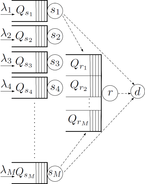
Figure 1: System Model

First, we describe the physical layer model. All wireless links are assumed to be stationary, frequency non-selective, and Rayleigh block fading. The fading coefficients $h_{m,n}$, where $m{\in}T$ and $n{\in}L$, are assumed to be constant during each slot duration, but change independently from one time slot to another according to a circularly symmetric complex Gaussian distribution with zero mean and variance $\rho_{m,n}^{2}$. All wireless links are corrupted by additive white Gaussian noise (AWGN) with zero mean and unit variance. All nodes transmit with fixed power $P$. An outage occurs when the instantaneous capacity of the link ($m$, $n$) is lower than the transmission rate $R$. Each link is characterized by the probability

$$f_{mn}=\mathbb{P}\{R<\log_{2}(1+P|h_{m,n}|^{2})\}=\exp\bigg{(}{-}\dfrac{2^{R}-1}{P\rho_{m,n}^{2}}\bigg{)}$$ (2)

which denotes the probability that the link ($m$, $n$) is not in outage. Let $g_{mn}^{I}$ denote the probability that the link ($m$, $n$) is not in outage in presence of interference from node $I$, where $m,I\in T$ and $n\in L$. In [9], the authors derived the same term but for symmetric configuration. We relax this assumption and re-derive the term to fit our model in Appendix A.

Next, we describe the medium access control layer model. Time is slotted with fixed slot duration, and the transmission of a packet takes exactly one time slot. Each source terminal has an infinite buffer (queue) to store its own incoming packets. Packet arrivals of the source terminals are independent and stationary Bernoulli processes with means $\lambda_{i}$ (packets per slot), where $i\in\{1,2,....,M\}$. The relay has $M$ relaying queues ($Q_{r_{1}}$, $Q_{r_{2}}$, . . ., $Q_{r_{M}}$) to store the packets of the source terminals that are not successfully decoded at the destination. Let $Q_{l}^{t}$ denote the number of packets in the $l$-th queue at the beginning of time slot $t$. The instantaneous evolution of the $l$-th queue length is given by

$$Q_{l}^{t+1}=(Q_{l}^{t}-Y_{l}^{t})^{+}+X_{l}^{t}$$ (3)

where $l\in\{s_{1},...s_{M},r_{1},...,r_{M}\}$ and $(x)^{+}{=}\max\{x,0\}$. The binary random variables $Y_{l}^{t}$ and $X_{l}^{t}$, denote the departures and arrivals of $Q_{l}$ in time slot $t$, respectively, and their values are either 0 or 1.

III Sensing-Based Cooperative Scheme

In this section, we introduce the proposed SBC scheme followed by its stability and delay analysis. We assume that the relay can sense the channel, and perfectly detect the idle time slots. Moreover, we assume that the errors and delay in packet acknowledgement (ACK) are negligible, which is reasonable for short length ACK packets as low rate codes can be employed in the feedback channel [4]. In the SBC scheme, the source terminals operate according to the following rules:

• Each terminal transmits the packet at the head of its queue in its assigned time slot, whenever the queue is not empty.

• If the destination decodes the packet successfully, it sends an ACK which can be heard by both the transmitting terminal and the relay. The terminal drops this packet upon hearing the ACK.

• If the destination does not receive the packet successfully but the relay does, then the relay stores this packet at the corresponding relaying queue and sends an ACK to the source terminal. Afterwards, the relay is responsible for conveying this packet to the destination.

• If a packet is received successfully by either the destination or the relay, the packet is removed from the terminal’s queue. Otherwise, the source terminal retransmits the packet in its next assigned time slot.

It is worth noting that if the relay and the destination decode a packet successfully, the relay does not store this packet in its queue because the packet is already delivered to the destination.

Next, we illustrate the transmission and reception policy of the relay using the SBC scheme. Let us consider the time slots allocated to the source terminal $s_{i}$. The relay takes one of the following two actions after sensing the channel to detect the queue state of $Q_{s_{i}}$.

• If $Q_{s_{i}}$ is empty, i.e. $s_{i}$ is not transmitting, the relay transmits the packet at the head of $Q_{r_{i}}$.

• If $Q_{s_{i}}$ is not empty, the relay transmits a packet from $Q_{r_{j}}$, where $j\in\{1,2,...,M\}$, with probability $\beta_{ij}$ or listens to source terminal transmission with probability $1{-}\sum\limits_{j=1}^{M}\beta_{ij}$.

Hereafter are some important remarks. First, the relay stores the packet of the source terminal if it decides to listen to the terminal’s transmission and successfully decodes the packet while the destination fails to decode it. Second, we assume that the relay is half duplex, and hence, it can not transmit and receive a packet in the same time slot. Thus, the relay can not receive packets when it decides to interfere with the source terminal.

From the given description of the proposed cooperative scheme, it is clear that the decision taken by the relay depends on the queue state of the source terminals, and this causes an interaction between the relay’s queues and those of the source terminals. Stability of interacting queues is complex [13], thus, we resort to using the dominant system approach. To perform the stability analysis of $s_{i}$, we assume that all other source terminals $s_{j}$, where $j\neq i$, are saturated, i.e, their queues always have packets. Moreover, we assume that $Q_{r_{i}}$ transmits a dummy packet whenever the relay decides to interfere with the source transmission and $Q_{r_{i}}$ is empty, where $i\in\{1,2,...,M\}$. This dominant system simplifies the stability analysis and provides an inner bound on the stability region.

III-A Stability Region Analysis

In this part, we characterize the stability region for the SBC scheme taking in consideration the dominant system described above. Then, we formulate an optimization problem to maximize the aggregate throughput and characterize the stability region via optimizing the values of $\{\beta_{ij}\}_{i,j{=}1}^{M}$ subject to constraints that ensure the stability of the system. The stability of the overall system requires the stability of each individual queue. From the definition in [18], the queue is stable if

$$\lim_{t\to\infty}\mathbb{P}\{Q_{l}^{t}<x\}=F(x)\enspace\text{and}\enspace\lim_{x\to\infty}F(x)=1$$ (4)

We can apply Loynes’ theorem to check the stability of a queue [19]. Loynes’ theorem states that if the arrival process and the service process of a queue are strictly stationary, then the queue is stable if and only if the average service rate is greater than the average arrival rate of the queue.

In the dominant system, a packet departs $Q_{s_{i}}$, where $i\in\{1,2,...,M\}$ in two cases. First, if it is successfully decoded by the destination when the relay decides to interfere with $s_{i}$ from one of its relaying queues. Second, if it is successfully decoded by at least one node, i.e., the destination or the relay when the relay decides to listen to $s_{i}$. Thus, the average service rate of $Q_{s_{i}}$ for certain $w_{i}$ is given by

$$\mu_{i}=w_{i}\Big{(}\sum\limits_{j=1}^{M}\beta_{ij}g_{s_{i}d}^{r}+(1-\sum\limits_{j=1}^{M}\beta_{ij})(f_{s_{i}d}+(1-f_{s_{i}d})f_{s_{i}r})\Big{)}.$$ (5)

For stability of $Q_{s_{i}}$, the following condition must be satisfied

$$\lambda_{i}<w_{i}\Big{(}\sum\limits_{j=1}^{M}\beta_{ij}g_{s_{i}d}^{r}+(1-\sum\limits_{j=1}^{M}\beta_{ij})(f_{s_{i}d}+(1-f_{s_{i}d})f_{s_{i}r})\Big{)}.$$ (6)

A packet arrives at $Q_{r_{i}}$ if the following two conditions are met. First, an outage occurs in the link between $s_{i}$ and the destination node while no outage occurs in the link between $s_{i}$ and the relay and this happens with probability $(1{-}f_{s_{i}d})f_{s_{i}r}$. Second, $Q_{s_{i}}$ is not empty and the relay decides to receive from $s_{i}$ and this happens with probability $\frac{\lambda_{i}}{\mu_{i}}(1-\sum\limits_{j=1}^{M}\beta_{ij})$. Thus, the average arrival rate of $Q_{r_{i}}$ is given by

$$\lambda_{r_{i}}=w_{i}(1{-}f_{s_{i}d})f_{s_{i}r}\frac{\lambda_{i}}{\mu_{i}}(1-\sum\limits_{j=1}^{M}\beta_{ij})$$ (7)

In the dominant system, the packet departs $Q_{r_{i}}$ in three cases. First, when $Q_{s_{i}}$ is empty a packet departs $Q_{r_{i}}$ if no outage occurs in the link between the relay and the destination. Second, when $Q_{s_{i}}$ is not empty a packet departs $Q_{r_{i}}$ if the relay decides to interfere with $s_{i}$ with a packet from $Q_{r_{i}}$. Third, if the relay decides to interfere with saturated source terminal $s_{j}$, where $j\neq i$, with a packet from $Q_{r_{i}}$. Thus, the average service rate of $Q_{r_{i}}$ can be expressed by

$$\mu_{r_{i}}{=}w_{i}\bigg{(}\Big{(}1{-}\frac{\lambda_{i}}{\mu_{i}}\Big{)}f_{rd}{+}\frac{\lambda_{i}}{\mu_{i}}\beta_{ii}g_{rd}^{s_{i}}\bigg{)}{+}\sum\limits_{j\neq i,j=1}^{M}w_{j}\beta_{ji}g_{rd}^{s_{j}}.$$ (8)

For the stability of $Q_{r_{i}}$, the service rate must be higher than the arrival rate, i.e., $\lambda_{r_{i}}<\mu_{r_{i}}$ , and hence, we have

$$\lambda_{i}<\frac{w_{i}f_{rd}+\sum\limits_{j=1,j\neq i}^{M}w_{j}\beta_{ji}g_{rd}^{s_{j}}}{w_{i}\Big{(}(1-\sum\limits_{j=1}^{M}\beta_{ij})(1-f_{s_{i}d})f_{s_{i}r}+f_{rd}-\beta_{ii}g_{rd}^{s_{i}}\Big{)}}\mu_{i}$$ (9)

Let $\lambda_{s}^{i}$ denote the maximum stable throughput for the i-th source terminal at a certain value of $w_{i}$. To guarantee the stability of the entire network the conditions in (6) and (9) must be satisfied. Hence, the maximum stable throughput is given by

$$\lambda_{s}^{i}<\min\{\mu_{i},\mu_{u_{i}}\}$$ (10)

where $\mu_{u_{i}}$ can be obtained easily from (9) as follows

$$\mu_{u_{i}}=\frac{w_{i}f_{rd}+\sum\limits_{j=1,j\neq i}^{M}w_{j}\beta_{ji}g_{rd}^{s_{j}}}{w_{i}\Big{(}(1-\sum\limits_{j=1}^{M}\beta_{ij})(1-f_{s_{i}d})f_{s_{i}r}+f_{rd}-\beta_{ii}g_{rd}^{s_{i}}\Big{)}}\mu_{i}$$ (11)

Next, we optimize the values of $\{\beta_{ij}\}_{i,j{=}1}^{M}$ to achieve the maximum weighted aggregate throughput of the network subject to constraints that ensure the stability of all queues. Thus, the optimization problem can written, for certain $w_{i}$, as follows

$$\underset{\enspace\enspace\{\beta\}_{i,j{=}1}^{M}}{\text{max}} \sum\limits_{i=1}^{M}x_{i}\lambda_{s}^{i}$$ (12)

subject to $$0\leq\sum\limits_{j=1}^{M}\beta_{ij}\leq 1, \enspace i\in\{1,2,...,M\}$$

$$\lambda_{s}^{i}\leq\mu_{i}, \enspace i\in\{1,2,...,M\}$$

$$\lambda_{s}^{i}\leq\mu_{u_{i}}, \enspace i\in\{1,2,...,M\}$$

$$0\leq\beta_{ij}\leq 1, \enspace i,j\in\{1,2,...,M\}$$

where $x_{i}$ is the weight assigned to $\lambda_{s}^{i}$. To obtain the stability region, we have to vary the value of each $x_{i}$, where $i\in\{1,2,...,M\}$, from zero to one for each $w_{i}$. Then vary $w_{i}$ also from zero to one to scan the whole stability region, i.e., the convex hull of all the obtained values of $\{\lambda_{s}^{i}\}_{i=1}^{M}$ provides the stability region. On the other hand, we set all values of $x_{i}$ by ones to calculate the maximum aggregate stable throughput of the network.

In the above problem, the summation in the first constraint is the probability that the relay transmits a packet from one of its relaying queue while $Q_{s_{i}}$ is not empty. The second and the third constraints guarantee the stability of the queues in the network. In order to solve this optimization problem, we define a new $M(M+1)$-dimensional vector $\boldsymbol{\beta}{=}[\beta_{11},...,\beta_{1M},...,\beta_{M1},...,\beta_{MM},\lambda_{s}^{1},...,\lambda_{s}^{M}]^{T}$ and rewrite the optimization problem, in the standard form [20], as follows

$$\underset{\boldsymbol{\beta}}{\text{min}} \boldsymbol{x}^{T}\boldsymbol{\beta}$$ (13)

s.t. $$0\leq\boldsymbol{b}_{i}^{T}\boldsymbol{\beta}\leq 1, \enspace i\in\{1,2,...,M\}$$

$$\boldsymbol{v}_{i}^{T}\boldsymbol{\beta}+u_{i}\leq 0, \enspace i\in\{1,2,...,M\}$$

$$\boldsymbol{\beta}^{T}\boldsymbol{A}_{i}\boldsymbol{\beta}+\boldsymbol{c}_{i}^{T}\boldsymbol{\beta}+d_{i}\leq 0, \enspace i\in\{1,2,...,M\}$$

$$\boldsymbol{0}\preceq\boldsymbol{\beta}\preceq\boldsymbol{1}$$

where $x{=}[0,0,...,0,-x_{1},...,-x_{M}]$, and the terms $\boldsymbol{v}_{i}$, $u_{i}$, $\boldsymbol{A}_{i}$, $\boldsymbol{c}_{i},$ and $d_{i}$ can be easily obtained from (5) and (11). From (5), the stability of $Q_{s_{i}}$ is represented by linear constraints in $\boldsymbol{\beta}$ while, from (11), the stability of $Q_{r_{i}}$ is represented by quadratic constraints in $\boldsymbol{\beta}$. The objective and the linear constraints are convex. However, the quadratic constraints are not convex because $\boldsymbol{A}_{i}$ is an indefinite matrix. In general, non-convex QCQP problems are NP hard [21], except for special cases such as those in [22]. Several methods have been proposed to approximate non-convex QCQP problems, including semi-definite relaxation (SDR) [21], the reformulation linearization technique (RLT) [23], and successive convex approximation (SCA) [24]. In our case, we use an iterative algorithm to obtain a good feasible solution as in [17]. We approximate the feasible region through a linear restriction of the non-convex parts of the constraints. The solution of the resulting optimization problem is then used to compute a new linearization and the procedure is repeated until convergence. Using the eigenvalue decomposition, the matrix $\boldsymbol{A}_{i}$ can be expressed as $\boldsymbol{A}_{i}=\boldsymbol{A}_{i}^{+}+\boldsymbol{A}_{i}^{-}$, where $\boldsymbol{A}_{i}^{+}\succeq 0$ and $\boldsymbol{A}_{i}^{-}\preceq 0$. For any $\boldsymbol{y}\in R^{M(M+1)\text{x}1}$, we can replace the non-convex constraint in (13) by the following convex one

$$\boldsymbol{\beta}^{T}\boldsymbol{A}_{i}^{+}\boldsymbol{\beta}+2\boldsymbol{y}^{T}\boldsymbol{A}_{i}^{-}\boldsymbol{\beta}+\boldsymbol{c}_{i}^{T}\boldsymbol{\beta}+d_{i}\leq\boldsymbol{y}^{T}\boldsymbol{A}_{i}^{-}\boldsymbol{y}$$ (14)

See [17] for more details. Thus, the non-convex problem is converted to a convex one, and we use Algorithm 1 to solve the optimization problem in (12).

1 Initialization: set $k=0$ and $\boldsymbol{y}_{0}=\boldsymbol{0}$.

2 Repeat

1. solve

   $$\underset{\boldsymbol{\beta}}{\text{min}} \boldsymbol{x}^{T}\boldsymbol{\beta}$$

   s. t. $$0\leq\boldsymbol{b}_{i}^{T}\boldsymbol{\beta}\leq 1$$

   $$\boldsymbol{v}_{i}^{T}\boldsymbol{\beta}+u_{i}\leq 0$$

   $$\boldsymbol{\beta}^{T}\boldsymbol{A}_{i}^{+}\boldsymbol{\beta}+2\boldsymbol{y}_{k}^{T}\boldsymbol{A}_{i}^{-}\boldsymbol{\beta}+\boldsymbol{c}_{i}^{T}\boldsymbol{\beta}+d_{i}\leq\boldsymbol{y}_{k}^{T}\boldsymbol{A}_{i}^{-}\boldsymbol{y}_{k}$$

   $$0\leq\boldsymbol{\beta}\leq 1,\enspace i\in\{1,2,...,M\}$$

2. Let $\boldsymbol{\beta}_{k}^{*}$ denote the optimal $\boldsymbol{\beta}$ obtained at the $k$-th iteration, and set $\boldsymbol{y}_{k+1}=\boldsymbol{\beta}_{k}^{*}$

3. Set $k=k+1$.

until convergence.

Algorithm 1 We use the FPP-SCA algorithm to achieve good feasible point

It is worth noting that we can use other techniques to solve this problem, but the FFP-SCA obtains good feasible point even for very large $M$. Moreover, a few iterations are required for convergence [17].

III-B Average Delay Characterization

In this subsection, we characterize the average delay for the dominant system of the SBC scheme. We derive an approximate expression of the delay as in [4], where we assume that the relay queues are discrete-time M/M/1 queues. If the packet is directly transmitted from the source terminal to the destination, it experiences a queueing delay only in the terminal’s queue. Alternatively, if the packet is delivered to the destination through the relay, this packet experiences two queuing delay; one in the terminal’s queue and the other in the relay’s queue. The packet experiences only the queueing delay at the source terminal with the following probability

$$\epsilon_{i}=w_{i}\frac{\Big{(}1{-}\sum\limits_{j=1}^{M}\beta_{ij}\Big{)}f_{s_{i}d}+\sum\limits_{j=1}^{M}\beta_{ij}g_{s_{i}d}^{r}}{\mu_{i}}$$ (15)

which is the probability that the packet is successfully decoded by the destination given that it is dropped from the source terminal. Thus, the average delay encountered by the packets of the $i$-th source terminal is given by

$$D_{i} =\epsilon_{i}T_{s_{i}}+(1-\epsilon_{i})(T_{s_{i}}+T_{r_{i}})$$

$$=T_{s_{i}}+(1-\epsilon_{i})T_{r_{i}}\enspace\enspace$$ (16)

where $T_{s_{i}}$ and $T_{r_{i}}$ denote the average queueing delays at $s_{i}$ and $r_{i}$, respectively. Since the arrival rates at $Q_{s_{i}}$ and $Q_{r_{i}}$ are given by $\lambda_{i}$ and $\lambda_{r_{i}}$, respectively, then applying Little’s law yields

$$T_{s_{i}}=N_{i}/\lambda_{i},\enspace T_{r_{i}}=N_{r_{i}}/\lambda_{r_{i}}$$ (17)

where $N_{i}$ and $N_{r_{i}}$ denote the average queue size of $Q_{s_{i}}$ and $Q_{r_{i}}$, respectively. The queues of the source terminals are discrete-time M/M/1 queues with Bernoulli arrivals and Geometrically distributed service rates, and we assume that $Q_{r_{i}}$ is a discrete-time M/M/1 queue. Thus, we can easily calculate $N_{s_{i}}$ and $N_{r_{i}}$, by applying the Pollaczek-Khinchine formula [25], as follows

$$N_{i}=\dfrac{-\lambda_{i}^{2}+\lambda_{i}}{\mu_{i}-\lambda_{i}},\enspace\enspace N_{r_{i}}=\dfrac{-\lambda_{r_{i}}^{2}+\lambda_{r_{i}}}{\mu_{r_{i}}-\lambda_{r_{i}}}\enspace$$ (18)

Substituting (17) and (18) in (III-B), we can write the average queueing delay for the $i$-th source terminal as

$$D_{i}=\frac{1-\lambda_{i}}{\mu_{i}-\lambda_{i}}+(1-\epsilon_{i})\frac{1-\lambda_{r_{i}}}{\mu_{r_{i}}-\lambda_{r_{i}}}$$ (19)

where the expressions of $\mu_{i}$ and $\lambda_{r_{i}}$, and $\mu_{r_{i}}$ are obtained in (5), (7), and (8), respectively.

IV Decision-Based Cooperative Scheme

In this section, we present the proposed DBC scheme together with its stability and delay analysis. In this scheme, the behavior of the source terminals is exactly the same as in the SBC scheme, where each source terminal transmits only in its assigned time slots. The source drops the packet if it hears an ACK from the relay or the destination, otherwise, the source retransmits the packet in the next assigned time slot. The main difference between the DBC and the SBC schemes is in the way the relay operates. In the SBC scheme, the relay decides its operation policy depending on the sensing information. However, in the DBC scheme, the relay does not sense the channel and it decides randomly either to transmit or to listen regardless the queue state of $s_{i}$. To illustrate the operation policy of the relay in the DBC scheme, let us consider the time slots allocated to $s_{i}$ where the relay takes one of the following actions:

• The relay transmits a packet from $Q_{r_{j}}$ with probability $\alpha_{ij}$, where $j\in\{1,2,..,M\}$

• The relay listens to the source transmission with probability $1-\sum\limits_{j=1}^{M}\alpha_{ij}$. The relay stores the source’s packet if the relay successfully decodes it while the destination fails.

When the relay decides to transmit without listening to the channel, the probability of successful transmission depends on the queue state of the source terminal because if the terminal’s queue is empty, there is a higher probability that the destination decodes the relay’s packet. Hence, it is clear that there is an interaction between the relay queues and those of the source terminals. To simplify the analysis, we assume the same dominant system used in the SBC scheme, where $Q_{r_{i}}$ transmits a dummy packet whenever the relay, randomly, decides to transmit a packet from $Q_{r_{i}}$ while this queue is empty. Furthermore, to perform the stability analysis of a certain source terminal, we assume that all other source terminals are saturated, i.e., their queues are not empty at any time slot. This dominant system simplifies the stability analysis and provides an inner bound on the stability region.

IV-A Stability Region Analysis

In this subsection, we follow the same steps as in the SBC scheme. First, we characterize the stability conditions for all the queues in the DBC scheme. Then, we formulate an optimization problem to maximize the weighted aggregate throughput and characterize the stability region by optimizing the values of $\{\alpha_{ij}\}_{i,j{=}1}^{M}$ under the stability constraints.

In the dominant system, a packet departs $Q_{s_{i}}$, where $i\in\{1,2,.....,M\}$, in two cases. First, if it is successfully decoded by at least one node, i.e., the destination or the relay when the relay decides to listen to $s_{i}$. Second, if it is successfully decoded by the destination when the relay decides to interfere with $s_{i}$. Thus, the average service rate of $Q_{s_{i}}$ for certain $w_{i}$ is given by

$$\mu_{i}=w_{i}\Big{(}(1-\sum\limits_{j=1}^{M}\alpha_{ij})(f_{s_{i}d}+(1-f_{s_{i}d})f_{s_{i}r})+\sum\limits_{j=1}^{M}\alpha_{ij}g_{s_{i}d}^{r}\Big{)}$$ (20)

For stability of $Q_{s_{i}}$, the following condition must be satisfied

$$\lambda_{i}<w_{i}\Big{(}(1-\sum\limits_{j=1}^{M}\alpha_{ij})(f_{s_{i}d}+(1-f_{s_{i}d})f_{s_{i}r})+\sum\limits_{j=1}^{M}\alpha_{ij}g_{s_{i}d}^{r}\Big{)}$$ (21)

A packet arrives at $Q_{r_{i}}$ if the following conditions are met. First, an outage occurs in the link between $s_{i}$ and the destination node while no outage occurs in the link between $s_{i}$ and the relay. Second, $Q_{s_{i}}$ is not empty which has a probability of $\lambda_{i}/\mu_{i}$, and the relay decides to listen to $s_{i}$ which happens with probability $1-\sum\limits_{j=1}^{M}\alpha_{ij}$. Thus, the average arrival rate of $Q_{r_{i}}$ is given by

$$\lambda_{r_{i}}=w_{i}(1-f_{s_{i}d})f_{s_{i}r}\frac{\lambda_{i}}{\mu_{i}}(1-\sum\limits_{j=1}^{M}\alpha_{ij})$$ (22)

In the dominant system, a packet departs from $Q_{r_{i}}$ in two cases. First, if the relay randomly decides to transmits a packet from $Q_{r_{i}}$ on the time slot allocated to $s_{i}$. In this case the packet departs $Q_{r_{i}}$ with probability $w_{i}\big{(}\alpha_{ii}f_{rd}(1-\frac{\lambda_{i}}{\mu_{i}}){+}\alpha_{ii}g_{rd}^{s_{i}}\frac{\lambda_{i}}{\mu_{i}}\big{)}$. Second, if the relay decides to transmits a packet from $Q_{r_{i}}$ in the time slot allocated to the saturated source terminal $s_{j}$, where $j\neq i$. In this case the packet departs $Q_{r_{i}}$ with probability $\sum\limits_{j{=}1,j\neq i}^{M}w_{j}\alpha_{ji}g_{rd}^{s_{j}}$. Thus, the average service rate of $Q_{r_{i}}$ can expressed by

$$\mu_{r_{i}}{=}w_{i}\Big{(}\alpha_{ii}f_{rd}(1-\frac{\lambda_{i}}{\mu_{i}}){+}\alpha_{ii}g_{rd}^{s_{i}}\frac{\lambda_{i}}{\mu_{i}}\Big{)}{+}\sum\limits_{j{=}1,j\neq i}^{M}w_{j}\alpha_{ji}g_{rd}^{s_{j}}$$ (23)

For the stability of $Q_{r_{i}}$, the service rate must be higher than the arrival rate, i.e., $\lambda_{r_{i}}<\mu_{r_{i}}$ , and hence, we have

$$\lambda_{i}<\frac{w_{i}\alpha_{ii}f_{rd}{+}\sum\limits_{j{=}1,j\neq i}^{M}w_{j}\alpha_{ji}g_{rd}^{s_{j}}}{w_{i}\Big{(}(1{-}\sum\limits_{j=1}^{M}\alpha_{ij})f_{s_{i}r}(1-f_{s_{i}d})+\alpha_{ii}f_{rd}-\alpha_{ii}g_{rd}^{s_{i}}\Big{)}}\mu_{i}$$ (24)

To guarantee the stability of the network the following condition must be satisfied

$$\lambda_{s}^{i}<\min\{\mu_{i},\mu_{u_{i}}\}$$ (25)

where $\mu_{u_{i}}$ obtained directly from (24) as follows

$$\mu_{u_{i}}=\frac{w_{i}\alpha_{ii}f_{rd}{+}\sum\limits_{j{=}1,j\neq i}^{M}w_{j}\alpha_{ji}g_{rd}^{s_{j}}}{w_{i}\Big{(}(1{-}\sum\limits_{j=1}^{M}\alpha_{ij})f_{s_{i}r}(1-f_{s_{i}d})+\alpha_{ii}f_{rd}-\alpha_{ii}g_{rd}^{s_{i}}\Big{)}}\mu_{i}$$ (26)

We can write the optimization problem to calculate the maximum weighted stable throughput of the network as

$$\underset{\enspace\enspace\{\alpha_{ij}\}_{i,j{=}1}^{M}}{\text{max}} \sum\limits_{i=1}^{M}x_{i}\lambda_{s}^{i}$$ (27)

subject to $$0\leq\sum\limits_{j=1}^{M}\alpha_{ij}\leq 1, \enspace i\in\{1,2,......,M\}$$

$$\lambda_{s}^{i}\leq\mu_{i}, \enspace i\in\{1,2,......,M\}$$

$$\lambda_{s}^{i}\leq\mu_{u_{i}}, \enspace i\in\{1,2,......,M\}$$

$$0\leq\alpha_{ij}\leq 1, \enspace i,j\in\{1,2,......,M\}$$

This optimization problem is exactly the same problem as that in the SBC scheme. Thus, we follow the same steps to solve this problem, and use the FPP-SCA algorithm to obtain good feasible solution.

IV-B Average Delay Characterization

In the DBC scheme, the source packets are either transmitted directly to the destination or through the relay. We define $\tau_{i}$, which is the probability that the packet is successfully decoded by the destination given that it is dropped from the $s_{i}$, as

$$\tau_{i}=w_{i}\frac{\Big{(}1{-}\sum\limits_{j=1}^{M}\alpha_{ij}\Big{)}f_{s_{i}d}+\sum\limits_{j=1}^{M}\alpha_{ij}g_{s_{i}d}^{r}}{\mu_{i}}$$ (28)

Thus, the packets of the $i$-th source terminal experience the following average delay

$$D_{i}=T_{s_{i}}+(1-\tau_{i})T_{r_{i}}$$ (29)

As in the SBC scheme, we can calculate $T_{s_{i}}$ and $T_{r_{i}}$ by assuming that $Q_{r_{i}}$ is a discrete-time M/M/1 queue and applying Pollaczek-Khinchine formula. Hence, we can write the average queueing delay for the $i$-th source terminal’s packets as

$$D_{i}=\frac{1-\lambda_{i}}{\mu_{i}-\lambda_{i}}+(1-\tau_{i})\frac{1-\lambda_{r_{i}}}{\mu_{r_{i}}-\lambda_{r_{i}}}$$ (30)

where the expressions of $\mu_{i}$, $\lambda_{r_{i}}$, and $\mu_{r_{i}}$ are obtained in (20), (22), and (23), respectively.

V Numerical Results

In this section, we evaluate the performance of the two proposed schemes for the case of two source terminals, i.e., $M{=}2$. We compare the performance of the SBC and DBC schemes with other cooperative schemes. First, we compare with the cooperative cognitive multiple-access (CCMA) scheme, proposed in [4], where the authors assume that the relay only transmits in the idle time slots. Moreover, the relay only helps the terminals which, on average, have worse channel condition than the relay itself. In other words, the relay assists the terminals whose outage probability to the destination satisfy $f_{rd}>f_{s_{i}d}$, where $i\in\{1,2,...,M\}$. Second, we compare with the DBC scheme while setting $g_{ij}^{I}{=}0$, i.e., the destination can decode only if there is one node is transmitting per time slot. We refer to this scheme by the collision model of the DBC scheme (CM-DBC). This scheme is important to illustrate how the MPR capability at the destination is essential in the absence of sensing at the relay. Third, we compare with the SBC and DBC schemes but with $\beta_{12}{=}\beta_{21}{=}0$ and $\alpha_{12}{=}\alpha_{21}{=}0$, respectively, to illustrate the effect of these probabilities and demonstrate the cases where their effect on the performance is essential. By setting $\beta_{12}{=}\beta_{21}{=}0$ and $\alpha_{12}{=}\alpha_{21}{=}0$, the relay can not transmit a relayed packet from $Q_{r_{i}}$ by interfering on $s_{j}$, where $i\neq j$.

We consider three cases for the channel conditions. In the first case, the system parameters are chosen as follows: $P{=}10,R{=}1$, $\rho_{s_{1},d}^{2}{=}0.02$, $\rho_{s_{2},d}^{2}{=}0.84$, $\rho_{s_{1},r}^{2}{=}0.97$, $\rho_{s_{2},r}^{2}{=}0.93$, and $\rho_{r,d}^{2}{=}0.03$. This case corresponds to an asymmetric channel situation, where the $r$-$d$ channel and the $s_{1}$-$d$ channel are weak while $s_{2}$-$d$ channel is strong. In Fig. 2, we plot the stability region for the cooperative schemes via varying the value of $w_{1}$ from zero to one by step $0.1$. It is obvious from the figure that the SBC scheme significantly outperforms the CCMA scheme. The rationale behind this enhancement is that in the CCMA scheme the relay is restricted to transmit its packets in the idle time slots only. On the other hand, the SBC scheme adds to the relay the capability to, simultaneously, transmit its packets with the source terminal while controlling the interference probabilistically. This capability expands the stability region.

It is worth noting that the two proposed schemes, SBC and DBC, can achieve exactly the same maximum stable throughput for $s_{2}$, while this is not the case for $s_{1}$. In the DBC scheme, the relay does not sense the channel, and hence, the relay may interfere with the source terminals. If the relay transmits a packet without sensing and interferes with $s_{2}$, the destination with high probability decodes the packet of $s_{2}$ first by treating the relay’s signal as noise, since the $s_{2}$-$d$ channel is strong, then decodes the relayed signal. This is not the case for $s_{1}$ because if the relay interferes with $s_{1}$ in the presence of these weak channels, $s_{1}$-$d$ and $r$-$d$, the destination most probably fails to decode both signals. The huge performance gap between the DBC scheme and the CM-DBC scheme demonstrates the importance of MPR capability at the destination in the absence of sensing capability at the relay. Removing the MPR capability causes a catastrophic reduction in the performance.

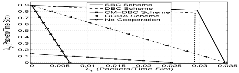
Figure 2: Stable throughput region for asymmetric channels configuration with weak relay-destination channel.

In Fig. 3, we use the same system parameters as in the former figure. We plot the maximum overall stable throughput versus $w_{1}$, which is the fraction of time allocated for $s_{1}$. This figure shows that as $w_{1}$ increases the maximum aggregate stable throughput of the network decreases. The reason behind this is that the maximum stable throughput for $s_{1}$ is equal to $0.035$ while that for $s_{2}$ is $0.9$. Consequently, as we allocate more time slots for $s_{2}$, the aggregate stable throughput of the network increases. Moreover, as shown in Fig. 2, the two proposed schemes, SBC and DBC, can achieve the same maximum stable throughput for $s_{2}$ which dominates the aggregate throughput for any $w_{1}$, and this is the reason why the aggregate throughput for the proposed schemes is close in Fig. 3.

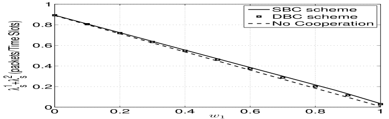
Figure 3: The maximum aggregate stable throughput for two source terminals in asymmetric channels configuration and weak relay-destination channel.

In the second case, Fig. 4, we plot the stability region for different cooperative schemes for the following system parameters: $P{=}10,R{=}1$, $\rho_{s_{1},d}^{2}{=}0.8$, $\rho_{s_{2},d}^{2}{=}0.08$, $\rho_{s_{1},r}^{2}{=}0.85$, $\rho_{s_{2},r}^{2}{=}0.9$, and $\rho_{r,d}^{2}{=}0.97$. This case corresponds to an asymmetric channel situation, where the channels $s_{1}$-$d$ and $r$-$d$ are strong while the channel $s_{2}$-$d$ is weak. It is important to note that the $r$-$d$ channel is stronger than that in the former case. In this case both proposed cooperative schemes achieve the same stability region, and hence, sensing does not increase the stability region of the system. In the DBC scheme, the relay transmits according a random experiment. If the relay decides, randomly, to interfere with $s_{1}$, the destination can decode both signals because both channels, $s_{1}$-$d$ and $r$-$d$, are strong. Alternatively, if the relay interferes with $s_{2}$, the destination most probably decodes the relay signal first, since $r$-$d$ channel is strong, then decodes the source signal. Consequently, the MPR capability at the destination decreases the need to detect idle time slots, and hence, both proposed schemes can achieve the same stability region. Removing the MPR capability at the destination, in absence of sensing, yields to the performance of the CM-DBC scheme which is much worse than that of the DBC scheme.

It is important to notice that both proposed schemes outperform the CCMA scheme which restricts the relay to send only in the idle time slots. Another insight from this figure is the importance of $\beta_{12}$ and $\beta_{21}$ in the SBC scheme and $\alpha_{12}$ and $\alpha_{21}$ in the DBC scheme to achieve this stability region. These probabilities have crucial effect in the asymmetric channel case as they enable the relay to utilize the time slots of one source to transmit the traffic of the other. Note that most of the packets of $s_{1}$ are transmitted directly to the destination due to the high gain of its direct channel. In contrast, $s_{2}$ suffers from low direct channel gain, so most of its packets are relayed. In the proposed schemes, the relay has the capability to interfere with $s_{1}$, which has high direct channel gain, and send a relayed packet of $s_{2}$, who suffers from low direct channel gain. This capability expands the stability region for both schemes.

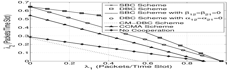
Figure 4: Stable throughput region for asymmetric channels configuration with strong relay-destination channel.

In Fig. 5, we plot the aggregate stable throughput of the two source network versus $w_{1}$. We use the same system parameters as in Fig. 4. It is obvious that the proposed schemes achieve higher aggregate throughput than that of the CCMA scheme. Unlike Fig. 3, the aggregate stable throughput increases as we allocate more time slots for $s_{1}$. In this case, the maximum stable throughput of $s_{1}$, $\lambda_{s}^{1}{=}0.98$, is greater than that of $s_{2}$, $\lambda_{s}^{2}{=}0.65$. Consequently, as $w_{1}$ increases the aggregate throughput of the network increases.

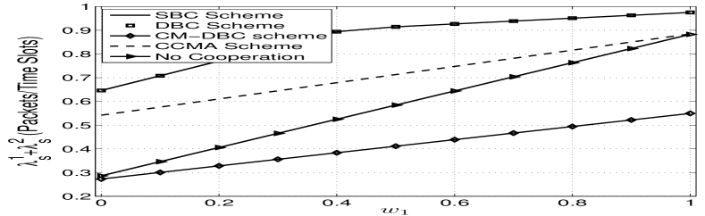
Figure 5: The maximum aggregate stable throughput for two source terminals in asymmetric channels configuration and strong relay-destination channel.

In the third case, Fig. 6, we plot the stability region for a roughly symmetric channel configuration where both direct links, $s_{1}$-$d$ and $s_{2}$-$d$, are strong. The system parameters are chosen as follows: $\rho_{s_{1},d}^{2}{=}0.75$, $\rho_{s_{2},d}^{2}{=}0.8$, $\rho_{s_{1},r}^{2}{=}0.63$, $\rho_{s_{2},r}^{2}{=}0.73$, and $\rho_{r,d}^{2}{=}0.85$. The SBC scheme still exceeds the CCMA scheme, however, in this case the role of of $\beta_{12}$ and $\beta_{21}$ diminishes due to the symmetric configuration. In this case, both source terminals have the same channel condition so the relay does not need to assist one source terminal at the expense of the other. Another insight from this figure is that, when the direct link channels are strong, we can achieve the performance of the CCMA scheme without even cooperation. However, the proposed schemes expand the stability region even when both direct links are strong.

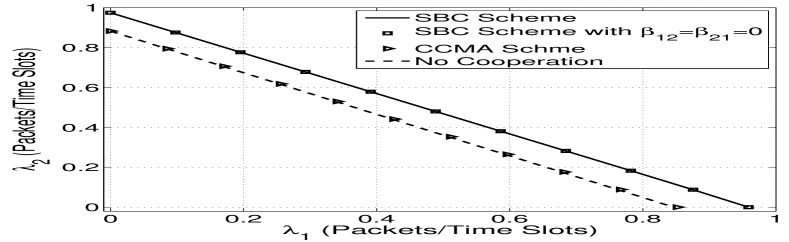
Figure 6: Stable throughput region for nearly symmetric channels configuration.

In Fig. 7, we illustrate how the proposed schemes respond when the channel capability to tolerate interference changes. We depict the effect of the transmission rate $R$ on the maximum aggregate stable throughput of the network for symmetric channel configuration. The parameters are chosen as follows: $w{=}0.5$, $\rho_{s_{1},d}^{2}{=}0.8$, $\rho_{s_{2},d}^{2}{=}0.8$, $\rho_{s_{1},r}^{2}{=}0.95$, $\rho_{s_{2},r}^{2}{=}0.95$, and $\rho_{r,d}^{2}{=}0.96$. It is clear that the stable throughput of the SBC and DBC schemes decrease slower than the CCMA and CM-DBC schemes. At low transmission rates, the channels can tolerate the interference, consequently, detecting the idle time slots is not important. It is obvious from the figure that the SBC and DBC schemes have the same performance for low transmission rates. As the transmission rate increases, the capability to sustain interference for all wireless channels decreases, and hence, it becomes essential for the relay to transmit only in the idle time slots. In the figure, as the transmission rate increases the performance of the two proposed schemes approaches to that of the CCMA scheme because the values of $\{\beta_{ij}\}_{i,j{=}1}^{2}$ and $\{\alpha_{ij}\}_{i,j{=}1}^{2}$ begin to decrease to limit the negative effect of interference. As we increase the transmission rate more, the channels can not sustain any interference. The values of $\{\beta_{ij}\}_{i,j{=}1}^{2}$ in the SBC scheme diminish to be almost zeros, and the relay is restricted to send only in the idle time slots. This means that the SBC scheme boils down to the CCMA scheme. On the other hand, for the DBC scheme, as the transmission rate increases, the ability that the destination decodes the transmission of two nodes simultaneously decreases, and hence, the DBC scheme turns to the CM-DBC scheme.

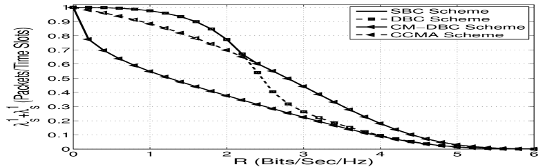
Figure 7: The maximum aggregate stable throughput versus the transmission rate for symmetric channels configuration.

In Figs. 8 and 9, we illustrate the delay performance of the proposed schemes. First, in Fig. 8, we plot the minimum average delay encountered by the packets of $s_{2}$, under the constraint that $\lambda_{s}^{1}{=}0.29$. Moreover, we use the same system parameters as in Fig. 2, where the two proposed schemes do not achieve the same stability region. The maximum stable throughputs for $s_{2}$, when $\lambda_{s}^{1}{=}0.29$, in the SBC and DBC schemes are $0.83$ and $0.77$, respectively. We do not plot the CCMA scheme to have a clear comparison between the plotted schemes, since the CCMA scheme performance is way worse than both. It is clear from the figure that the delay performance of the two proposed schemes in this case is close to each other for low $\lambda_{2}$. However, the SBC scheme delay performance slightly exceeds that of the DBC scheme. As $\lambda_{2}$ increases the SBC scheme begins to significantly outperform the DBC scheme. It is obvious that the results obtained through queue simulation are very close to the results of the closed-form expressions derived in (19) and (30). This validates the soundness of the mathematical model. Moreover, the trade-off between the stable throughput and the average delay is clear where as the throughput increases the delay increases.

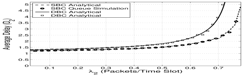
Figure 8: The average delay encountered by the packets of $s_{2}$ for asymmetric channels configuration with weak relay-destination channel.

In Fig. 9, we plot the minimum delay for $s_{1}$ when $\lambda_{s}^{2}{=}0.81$. We use the same system parameters as those in Fig. 4, where the two proposed schemes achieve the same stability region. In this case, the maximum stable throughput for $s_{2}$ in the SBC, DBC and CCMA schemes are $0.13$, $0.13$, and $0.038$, respectively. The figure depicts that the proposed schemes significantly outperform the CCMA scheme. The rationale behind this is that the CCMA scheme allocates a large fraction of the time slots for $s_{2}$ to satisfy the constraint $\lambda_{s}^{2}{=}0.81$, besides, the relay transmits only in the idle time slots. Consequently, the delay performance of the CCMA is much worse than that of the two proposed schemes. It is worth noting that even when the two proposed schemes can achieve the same stability region, the delay performance of the SBC scheme outperforms that of the DBC scheme. This is because the SBC scheme exploits the idle time slots to transmit the relayed packets, and the capability of the channel to sustain the interference to send simultaneously with the source terminal. Consequently, the SBC scheme exceeds the DBC scheme that exploits only the capability of the channels to tolerate interference.

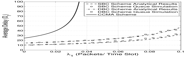
Figure 9: The average delay encountered by the packets of $s_{1}$ for asymmetric channels configuration with strong relay-destination channel.

VI Sensing at the relay versus MPR at the destination

In this section, we illustrate how the MPR capability at the destination can compensate for the lack of sensing at the relay. Moreover, we derive the condition under which the two proposed schemes achieve exactly the same maximum stable throughput, $\lambda_{s}^{i}$. In this part, we assume that $w_{1}{=}1$, and hence, all time slots are allocated to $s_{1}$, i.e., we have only one source terminal $s_{1}$.

Theorem 1.

The maximum stable throughput for the two proposed schemes is given by

$$\lambda_{s}^{1^{*}}=(1{-}\frac{T_{1}}{T_{1}{+}g_{rd}^{s_{1}}})(f_{s_{1}d}{+}T_{1}){+}\frac{T_{1}}{T_{1}{+}g_{rd}^{s_{1}}}g_{s_{1}d}^{r}$$ (31)

if the following condition is satisfied

$$f_{rd}-g_{rd}^{s_{1}} \leq\min\bigg{\{}\frac{g_{s_{1}d}^{r}(T_{1}+f_{rd})}{T_{1}+f_{s_{1}d}},$$ (32)

$$\frac{(T_{1}+g_{rd}^{s_{1}})^{2}(f_{s_{1}d}+T_{1})}{T_{1}(f_{s_{1}d}+T_{1}-g_{s_{1}d}^{r})}{-}(T_{1}+2g_{rd}^{s_{1}})\bigg{\}}$$

where $T_{1}{=}(1{-}f_{s_{1}d})f_{s_{1}r}$.

Proof of Theorem 1.

In the SBC scheme, we can rewrite the stability condition in (10) for $w_{1}{=}1$ as

$$\lambda_{s}^{1}<\min\{\mu_{1}^{\text{SBC}},\mu_{u_{1}}^{\text{SBC}}\}$$ (33)

where

$$\mu_{1}^{\text{SBC}} =(1-\beta_{11})(f_{s_{1}d}+T_{1})+\beta_{11}g_{s_{1}d}^{r}$$ (34)

$$\mu_{u_{1}}^{\text{SBC}} =\frac{f_{rd}}{(1-\beta_{11})T_{1}+f_{rd}-\beta_{11}g_{rd}^{s_{1}}}\mu_{1}^{\text{SBC}}$$ (35)

The optimization problem in (12) can be written as

$$\underset{\beta_{11}}{\text{max}} \min\{\mu_{1}^{\text{SBC}},\mu_{u_{1}}^{\text{SBC}}\}$$ (36)

subject to $$0\leq\beta_{11}\leq 1$$

Lemma 1.

If the following condition is satisfied

$$f_{rd}-g_{rd}^{s_{1}}\leq\frac{g_{s_{1}d}^{r}(T_{1}+f_{rd})}{T_{1}+f_{s_{1}d}},$$ (37)

the solution of the optimization problem in (36) is given by

$$\lambda_{s}^{1^{*}}=(1{-}\frac{T_{1}}{T_{1}{+}g_{rd}^{s_{1}}})(f_{s_{1}d}{+}T_{1}){+}\frac{T_{1}}{T_{1}{+}g_{rd}^{s_{1}}}g_{s_{1}d}^{r}$$ (38)

Proof.

See Appendix B ∎

For the DBC scheme, we can rewrite the the optimization problem in (27) as follows

$$\underset{\alpha_{11}}{\text{max}} \min\{\mu_{1}^{\text{DBC}},\mu_{u_{1}}^{\text{DBC}}\}$$ (39)

subject to $$0\leq\alpha_{11}\leq 1$$

where

$$\mu_{1}^{\text{DBC}} =(1-\alpha_{11})(f_{s_{1}d}+T_{1}){+}\alpha_{11}g_{s_{1}d}^{r}$$ (40)

$$\mu_{u_{1}}^{\text{DBC}} =\frac{\alpha_{11}f_{rd}}{(1-\alpha_{11})T_{1}+\alpha_{11}f_{rd}-\alpha_{11}g_{rd}^{s_{1}}}\mu_{1}^{\text{DBC}}$$ (41)

Lemma 2.

If the following condition is satisfied

$$f_{rd}-g_{rd}^{s_{1}}\leq\frac{(T_{1}+g_{rd}^{s_{1}})^{2}(f_{s_{1}d}+T_{1})}{T_{1}(f_{s_{1}d}+T_{1}-g_{s_{1}d}^{r})}{-}(T_{1}+2g_{rd}^{s_{1}})$$ (42)

the maximum stable throughput for $s_{1}$ in the DBC scheme, which is the solution of the problem in (39), is given by

$$\lambda_{s}^{1^{*}}=(1{-}\frac{T_{1}}{T_{1}{+}g_{rd}^{s_{1}}})(f_{s_{1}d}{+}T_{1}){+}\frac{T_{1}}{T_{1}{+}g_{rd}^{s_{1}}}g_{s_{1}d}^{r}$$ (43)

Proof.

See Appendix C ∎

The conditions (37) and (42) establish the result in (31) and (32).

∎

Theorem 1 states that if the values of $f_{rd}$ and $g_{rd}^{s_{1}}$ are close, i.e., they satisfy the condition in (32), the two proposed schemes achieve exactly the same maximum throughput. The values $f_{rd}$ and $g_{rd}^{s_{1}}$ depend on the variance of two channels; $s_{1}$-$d$ and $r$-$d$. From the definitions in (2) and (44), the value of $g_{rd}^{s_{1}}$ is close to that of $f_{rd}$ in two cases. First, if the two channels, $s_{1}$-$d$ and $r$-$d$, are strong, i.e., the destination can decode both signals with high probability. Second, if at least one of the channels, $r$-$d$ or $s_{1}$-$d$, is strong, i.e., the destination can decode the strong signal first then the weak one.

We can easily map the insights from the obtained condition in (32) to that in Fig. 2 and Fig. 4. First, in Fig. 2, the condition in (32) is violated for $s_{1}$, where we have two weak channels, $s_{1}$-$d$ and $r$-$d$. Hence, the maximum stable throughput of $s_{1}$ in the SBC scheme is greater than that in the DBC scheme. Alternatively, in the same figure, the condition is satisfied for $s_{2}$, where we have one strong channel $s_{2}$-$d$. Thus, the maximum stable throughput of $s_{2}$ in the SBC scheme is exactly the same as that in the DBC scheme. Second, in Fig. 4, the condition is satisfied for both users, hence, the maximum stable throughput for $s_{1}$ and $s_{2}$ is the same for the two proposed schemes. Moreover, the two schemes achieve the same stability region. From these results, we can realize that the MPR capability at the destination can compensate for the need for sensing to detect the idle time slots, if there is at least one strong channel to the destination. The strong channel facilitates the decoding at the destination, and mitigates the need of the relay to send only in empty channels.

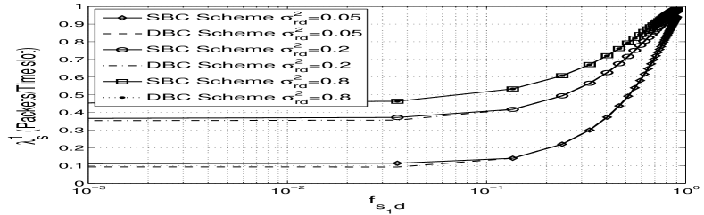
Figure 10: The effect of the channels, $s_{1}$-$d$ and $r$-$d$, on the maximum stable throughput of the two proposed schemes for $w_{1}{=}1$ for three fixed values for $r$-$d$ channel variance.

In Fig. 10, we show numerically different channel variances that satisfy the condition in (32). We plot the maximum stable throughput of $s_{1}$ versus $f_{s_{1}d}$ by varying $\sigma_{s_{1}d}^{2}$ from zero to one for three fixed values $\sigma_{rd}^{2}$. The system parameters of this figure are chosen as follows: $w_{1}{=}1$, $P{=}10$, $R{=}1$, and $\rho_{s_{1},r}^{2}{=}0.8$. In the first case, where $\sigma_{rd}^{2}{=}0.05$, the two proposed schemes achieve the same stable throughput approximately at $f_{s_{1}d}{=}0.15$. As we increase $\sigma^{2}_{rd}$, the performance of the two proposed schemes becomes closer than that of the former case. Ultimately, for the case of strong $r$-$d$ channel $\sigma_{rd}^{2}{=}0.8$, the two proposed schemes almost achieve the same performance for any $\sigma_{s_{1}d}^{2}$, and this result emphasises the insights obtained from the condition in (32).

VII Conclusion

In this paper, we have proposed two cooperation schemes, and studied their impact at the medium access layer metrics such as stable throughput and average delay. In the SBC scheme, the relay senses the channel at the beginning of each time slot, and it decides either to transmit or receive packets depending on the sensing outcome. On the other hand, in the DBC scheme, the relay does not sense the channel, and it decides its operation in a random fashion. For each scheme, we derived the stability conditions for each queue in the system and characterized the stability region. Furthermore, we derived approximate expression for the average delay encountered by the packets. We illustrated how the SBC scheme significantly outperforms existing cooperative schemes. The SBC scheme exploits the available resources more efficiently than other cooperative schemes because the relay not only utilizes the idle time slots, but also interferes with the source terminals in a mild way to mitigate the adverse effects of interference.

Moreover, we demonstrated that the MPR capability at the destination can compensate for the relay need to sense the channel. Although the relay in the DBC scheme does not sense the channel, our results show that the DBC scheme can achieve, under a certain condition, the same stability region as that of the SBC scheme.

Appendix A

Derivation of $g_{mn}^{I}$

The term $g_{mn}^{I}$ denotes the probability that the link ($m,n$) is not in outage in presence of interference from node I. Thus, we can express it as follows

$$g_{mn}^{I}=v_{mn}^{I}+(1-v_{mn}^{I})h_{mn}^{I}$$ (44)

where $v_{mn}^{I}$ is the probability that the node $n\in L$ successfully decodes both packets transmitted from $m\in T$ and $I\in T$, on the other hand, $h_{mn}^{I}$ is the probability that the node $n$ successfully decodes the packet transmitted from $m$ by treating $I$ as noise. Let X and Y be two independent exponential random variables with parameters $\gamma_{1}$ and $\gamma_{2}$, respectively, and $p(x)$ and $p(y)$ be their probability density functions. We define two deterministic variables $\eta$ and $\eta_{1}$. To derive the expression of $v_{mn}^{I}$, we first define the region

$$\Re(\eta,\eta_{1}) =\{(x,y):x>\eta\cap y>\cap x{+}y>\eta_{1}\}$$ (45)

$$=\{(x,y):x>\eta\cap y>\max[\eta,\eta_{1}-x]\}$$

$$=\{(x,y):\eta_{1}-\eta\geq x\geq\eta\cap y>\eta_{1}-x\}$$

$$\cup\{(x,y):x>\eta_{1}-\eta\cap y>\eta\},$$

then, we figure the following integration

$$V(\eta,\eta_{1},\gamma_{1},\gamma_{2}){=} \iint\limits_{\Re(\eta,\eta_{1})}p(x,y)dxdy$$ (46)

$${=} \int\limits_{\eta}^{\eta_{1}-\eta}p(x)\int\limits_{\eta-x}^{\infty}p(y)\enspace dydx$$

$${+} \int\limits_{\eta_{1}-\eta}^{\infty}p(x)\int\limits_{\eta}^{\infty}p(y)\enspace dydx$$

$${=} \frac{\gamma_{1}e^{\gamma_{2}\eta_{1}}}{\gamma_{1}{-}\gamma_{2}}\leavevmode\resizebox{272.45874pt}{}{$(\exp\big{(}{-}(\gamma_{1}{-}\gamma_{2})\eta\big{)}{-}\exp({-}(\gamma_{1}{-}\gamma_{2})(\eta_{1}{-}\eta)))$}$$

$${+} \exp(\eta_{1}\gamma_{1}+\eta(\gamma_{2}{-}\gamma_{1}))$$

Hence, we have

$$v_{mn}^{I}=V(\frac{2^{R}{-}1}{P},\frac{2^{2R}{-}1}{P},\frac{1}{\rho_{m,n}^{2}},\frac{1}{\rho_{I,n}^{2}}).$$ (47)

To derive the expression of $h_{mn}^{I}$, we first perform the following integration

$$H(\eta,\gamma_{1},\gamma_{2}) =\mathbb{P}\{R<\log(1+\frac{Px}{Py+1})\}$$ (48)

$$=\int\limits_{0}^{\infty}\exp\big{(}\frac{(2^{R}-1)(Py+1)\gamma_{1}}{P}\big{)}p(y)dy$$

$$=\frac{\gamma_{2}\exp(-\eta\gamma_{1})}{\gamma_{2}+P\gamma_{1}\eta}.$$

Hence, the probability $h_{mn}^{I}$ is given by

$$h_{mn}^{I}=H(\frac{2^{R}-1}{P},\frac{1}{\rho_{m,n}^{2}},\frac{1}{\rho_{I,n}^{2}})$$ (49)

Appendix B

Proof of Lemma 1

Taking the derivative of $\mu_{1}^{\text{SBC}}$ and $\mu_{u_{1}}^{\text{SBC}}$ with respect to $\beta_{11}$ yields the following

$$\frac{\partial\mu_{1}^{\text{SBC}}}{\partial\beta_{11}} =g_{s_{1}d}^{r}-f_{s_{1}d}-T_{1}$$ (50)

$$\frac{\partial\mu_{u_{1}}^{\text{SBC}}}{\partial\beta_{11}} {=}\frac{f_{rd}(g_{s_{1}d}^{r}{-}T_{1}{-}f_{s_{1}d})(T_{1}{+}f_{rd}{-}\beta_{11}(T_{1}{+}g_{rd}^{s_{1}}))}{\big{(}(1-\beta_{11})T_{1}+f_{rd}-\beta_{11}g_{rd}^{s_{1}}\big{)}^{2}}$$ (51)

$$+\frac{f_{rd}(T_{1}+g_{rd}^{s_{1}})(T_{1}{+}f_{s_{1}d}{+}\beta_{11}(g_{s_{1}d}^{r}+T_{1}-f_{s_{1}d}))}{\big{(}(1-\beta_{11})T_{1}+f_{rd}-\beta_{11}g_{rd}^{s_{1}}\big{)}^{2}}$$

From (50), we can see that $\mu_{1}^{\text{SBC}}$ is a monotonically decreasing function in $\beta_{11}$ because, from definition, $f_{s_{1}d}$ is greater than $g_{s_{1}d}^{r}$. On the other side, from (51), we can show that $\mu_{u_{1}}^{\text{SBC}}$ is monotonically increasing in $\beta_{11}$ if the following condition is satisfied

$$f_{rd}-g_{rd}^{s_{1}}\leq\frac{g_{s_{1}d}^{r}(T_{1}+f_{rd})}{T_{1}+f_{s_{1}d}}.$$ (52)

Since the value of $\mu_{1}^{\text{SBC}}$ at $\beta_{11}{=}{0}$ is greater than the value of $\mu_{u_{1}}^{\text{SBC}}$ at $\beta_{11}{=}{0}$ and $\mu_{1}^{\text{SBC}}$ decreases monotonically with $\beta_{11}$ while $\mu_{u_{1}}^{\text{SBC}}$ increases when (52) is satisfied, the optimal solution of (36) occurs when $\mu_{1}^{\text{SBC}}=\mu_{u_{1}}^{\text{SBC}}$. Thus, under the above condition in (52), the optimum $\beta_{11}$ is given by

$$\beta_{11}^{*}=\frac{T_{1}}{T_{1}+g_{rd}^{s_{1}}}$$ (53)

and, hence, the maximum stable throughput for $s_{1}$ is given by

$$\lambda_{s}^{1^{*}}=(1{-}\frac{T_{1}}{T_{1}{+}g_{rd}^{s_{1}}})(f_{s_{1}d}{+}T_{1}){+}\frac{T_{1}}{T_{1}{+}g_{rd}^{s_{1}}}g_{s_{1}d}^{r}$$ (54)

Appendix C

Proof of Lemma 2

It is clear, from (40), that $\mu_{1}^{\text{DBC}}$ decreases monotonically with $\alpha_{11}$. On the other hand, the derivative of $\mu_{u_{1}}^{\text{DBC}}$ with respect to $\alpha_{11}$ is given by

$$\frac{\partial\mu_{u_{1}}^{\text{DBC}}}{\partial\alpha_{11}} {=}\leavevmode\resizebox{422.77661pt}{}{$\frac{f_{rd}(T_{1}{+}f_{s_{1}d}{+}2\alpha_{11}(g_{s_{1}d}^{r}{-}T_{1}{-}f_{s_{1}d}))(T_{1}{+}\alpha_{11}(f_{rd}{-}T_{1}{-}g_{rd}^{s_{1}}))}{((1-\alpha_{11})T_{1}+\alpha_{11}f_{rd}-\beta_{11}g_{rd}^{s_{1}})^{2}}$}$$

$${-}\leavevmode\resizebox{422.77661pt}{}{$\frac{f_{rd}(f_{rd}-T_{1}-g_{rd}^{s_{1}})(\alpha_{11}(f_{s_{1}d}+T_{1})+\alpha_{11}^{2}(g_{s_{1}d}^{r}-f_{s_{1}d}-T_{1}))}{((1-\alpha_{11})T_{1}+\alpha_{11}f_{rd}-\alpha_{11}g_{rd}^{s_{1}})^{2}}$}$$ (55)

It is obvious from (41) that $\mu_{u_{1}}^{\text{DBC}}$ is a quadratic over linear function in $\alpha_{11}$, and hence, it is a concave function in $\alpha_{11}$ for the range of $\alpha_{11}$ from zero to one [20]. Besides, $\mu_{u_{1}}^{\text{DBC}}$ increases at $\alpha_{11}{=}0$, because the slope of $\mu_{u_{1}}^{\text{DBC}}$ at $\alpha_{11}{=}0$ is positive and given by

$$\frac{f_{rd}T_{1}(T_{1}+f_{s_{1}d})}{((1-\alpha_{11})T_{1}+\alpha_{11}f_{rd}-\alpha_{11}g_{rd}^{s_{1}})^{2}}$$ (56)

Note that the two functions $\mu_{1}^{\text{DBC}}$ and $\mu_{u_{1}}^{\text{DBC}}$ satisfy the following three conditions. First, the value of $\mu_{1}^{\text{DBC}}$ at $\alpha_{11}={0}$ is greater than the value of $\mu_{u_{1}}^{\text{DBC}}$ at the same point. Second, $\mu_{1}^{\text{DBC}}$ is monotonically decreasing function in $\alpha_{11}$. Third, $\mu_{u_{1}}^{\text{DBC}}$ is concave function with positive slope at $\alpha_{11}{=}0$. Therefore, the optimum value of $\alpha_{11}$ is obtained at the intersection point between $\mu_{1}^{\text{DBC}}$ and $\mu_{u_{1}}^{\text{DBC}}$ if the slope of $\mu_{u_{1}}^{\text{DBC}}$ is positive at this point because this means that $\mu_{u_{1}}^{\text{DBC}}$ increases monotonically with $\alpha_{11}$ from $\alpha_{11}{=0}$ until the intersection point. $\mu_{u_{1}}^{\text{DBC}}$ has a positive slope at the intersection point if the following condition satisfied

$$f_{rd}-g_{rd}^{s_{1}}\leq\frac{(T_{1}+g_{rd}^{s_{1}})^{2}(f_{s_{1}d}+T_{1})}{T_{1}(f_{s_{1}d}+T_{1}-g_{s_{1}d}^{r})}{-}(T_{1}+2g_{rd}^{s_{1}})$$ (57)

Under the above condition, the optimum solution of (39) occurs when $\mu_{1}^{\text{DBC}}{=}\mu_{u_{1}}^{\text{DBC}}$, hence the optimum value of $\alpha_{11}$ is given by

$$\alpha_{11}^{*}=\frac{T_{1}}{T_{1}+g_{rd}^{s_{1}}}$$ (58)

and, the maximum stable throughput for $s_{1}$ is given by

$$\lambda_{s}^{1^{*}}=(1{-}\frac{T_{1}}{T_{1}{+}g_{rd}^{s_{1}}})(f_{s_{1}d}{+}T_{1}){+}\frac{T_{1}}{T_{1}{+}g_{rd}^{s_{1}}}g_{s_{1}d}^{r}$$ (59)

which is exactly the same stable throughput for the SBC scheme in (54).

References

- [1] J. Mitola and G. Q. Maguire Jr, “Cognitive radio: making software radios more personal,” Personal Communications, IEEE, vol. 6, no. 4, pp. 13–18, 1999.
- [2] J. N. Laneman, D. N. Tse, and G. W. Wornell, “Cooperative diversity in wireless networks: Efficient protocols and outage behavior,” IEEE Transactions on Information Theory, vol. 50, no. 12, pp. 3062–3080, 2004.
- [3] A. Sendonaris, E. Erkip, and B. Aazhang, “User cooperation diversity. part i. system description,” IEEE Transactions on Communications, vol. 51, no. 11, pp. 1927–1938, 2003.
- [4] A. K. Sadek, K. R. Liu, and A. Ephremides, “Cognitive multiple access via cooperation: protocol design and performance analysis,” IEEE Transactions on Information Theory, vol. 53, no. 10, pp. 3677–3696, 2007.
- [5] B. Rong and A. Ephremides, “Cooperation above the physical layer: the case of a simple network,” in IEEE International Symposium on Information Theory. IEEE, 2009, pp. 1789–1793.
- [6] S. Ghez, S. Verdu, and S. C. Schwartz, “Stability properties of slotted aloha with multipacket reception capability,” IEEE Transactions on Automatic Control, vol. 33, no. 7, pp. 640–649, 1988.
- [7] A. ParandehGheibi, M. Médard, A. Ozdaglar, and A. Eryilmaz, “Information theory vs. queueing theory for resource allocation in multiple access channels,” in IEEE Personal Indoor and Mobile Radio Communications, Septemper 2008, pp. 1–5.
- [8] V. Naware, G. Mergen, and L. Tong, “Stability and delay of finite-user slotted aloha with multipacket reception,” IEEE Transactions on Information Theory, vol. 51, no. 7, pp. 2636–2656, 2005.
- [9] I. Krikidis, N. Devroye, and J. S. Thompson, “Stability analysis for cognitive radio with multi-access primary transmission,” IEEE Transactions on Wireless Communications, vol. 9, no. 1, pp. 72–77, 2010.
- [10] A. Fanous and A. Ephremides, “Stable throughput in a cognitive wireless network,” IEEE Transactions on Selected Areas in Communications, vol. 31, no. 3, pp. 523–533, 2013.
- [11] B. Rong and A. Ephremides, “Cooperative access in wireless networks: stable throughput and delay,” IEEE Transactions on Information Theory, vol. 58, no. 9, pp. 5890–5907, 2012.
- [12] M. Ashour, A. A. El-Sherif, T. ElBatt, and A. Mohamed, “Cooperative access in cognitive radio networks: Stable throughput and delay tradeoffs,” arXiv preprint arXiv:1309.1200, 2013.
- [13] B. S. Tsybakov and V. A. Mikhailov, “Ergodicity of a slotted aloha system,” Problemy Peredachi Informatsii, vol. 15, no. 4, pp. 73–87, 1979.
- [14] R. R. Rao and A. Ephremides, “On the stability of interacting queues in a multiple-access system,” IEEE Transactions on Information Theory, vol. 34, no. 5, pp. 918–930, 1988.
- [15] M. Sidi and A. Segall, “Two interfering queues in packet-radio networks,” IEEE Transactions on Communications, vol. 31, no. 1, pp. 123–129, 1983.
- [16] Y. Huang and D. Palomar, “Randomized algorithms for optimal solutions of double-sided qcqp with applications in signal processing,” IEEE Transactions on Signal Processing, vol. 62, no. 5, pp. 1093–1108, 2014.
- [17] O. Mehanna, K. Huang, B. Gopalakrishnan, A. Konar, and N. D. Sidiropoulos, “Feasible point pursuit and successive approximation of non-convex qcqps,” arXiv preprint arXiv:1410.2277, 2014.
- [18] W. Szpankowski, “Stability conditions for some distributed systems: Buffered random access systems,” Advances in Applied Probability, vol. 26, pp. 498–515, 1994.
- [19] R. Loynes, “The stability of a queue with non-independent inter-arrival and service times,” vol. 58, no. 3. Cambridge Univ Press, 1962, pp. 497–520.
- [20] S. P. Boyd and L. Vandenberghe, Convex optimization. Cambridge university press, 2004.
- [21] L. Vandenberghe and S. Boyd, “Semidefinite programming,” SIAM review, vol. 38, no. 1, pp. 49–95, 1996.
- [22] Y. Huang and D. P. Palomar, “Rank-constrained separable semidefinite programming with applications to optimal beamforming,” IEEE Transactions on Signal Processing, vol. 58, no. 2, pp. 664–678, 2010.
- [23] H. D. Sherali and W. P. Adams, A reformulation-linearization technique for solving discrete and continuous nonconvex problems. Springer, 1998, vol. 31.
- [24] A. Beck, A. Ben-Tal, and L. Tetruashvili, “A sequential parametric convex approximation method with applications to nonconvex truss topology design problems,” IEEE Transactions on Global Optimization, vol. 47, no. 1, pp. 29–51, 2010.
- [25] L. Kleinrock, “Queueing systems. volume 1: Theory,” 1975.