On the novelty, efficacy, and significance of weak measurements for quantum tomography

Abstract

The use of weak measurements for performing quantum tomography is enjoying increased attention due to several recent proposals. The advertised merits of using weak measurements in this context are varied, but are generally represented by novelty, increased efficacy, and foundational significance. We critically evaluate two proposals that make such claims and find that weak measurements are not an essential ingredient for most of their advertised features.

I Introduction

The business of quantum state tomography is converting multiple copies of an unknown quantum state into an estimate of that state by performing measurements on the copies. The naïve approach to the problem involves measuring different observables (represented by Hermitian operators) on each copy of the state and constructing the estimate as a function of the measurement outcomes (corresponding to different eigenvalues of the observables). Though tomography can be performed in such a way, there are more general ways of interrogating the ensemble; indeed, generalizations such as ancilla-coupled Dar2002 and joint Mas1993 measurements lead one to evaluate the problem of tomography from the perspective of generalized measurements Nie2010 , an approach which has yielded many optimal tomographic strategies Hol1982 ; Hra1997 ; BagBalGil2006 ; Blu2010 ; Gro2010 .

An interesting subclass of generalized measurements is the class of weak measurements BarLanPro1982 ; CavMil1987 ; DarYue1996 ; FucJac2001 ; OreBru2005 . Figure 1 gives a quantum-circuit description of a weak measurement. Weak measurements are often the only means by which an experimentalist can probe her system, thus making them of practical interest ChuGerKub1998 ; SmiSilDeu2006 ; GillettDaltonLanyon2010 ; SayDotZho2011 ; VijMacSli2012 ; CamFluRoc2013 ; CooRioDeu2014 . Sequential weak measurements are also useful for describing continuous measurements WisemanMilburn2010 .

Weak measurements are also central in the more contentious formalism of weak values AAV1988 . In particular, the technique of weak-value amplification HostenKwiat2008 has generated much debate over its metrological utility StrubiBruder2013 ; Knee2013a ; TanYam2013 ; FerCom2013 ; Knee2013b ; ComFerJia13a ; ZhaDatWam13 ; DresselMalikMiatto2014 ; JordanMartinez-RinconHowell2014 ; LeeTsutsui2014 ; KneComFerGau14 .

The two proposals we review in this paper assert that it is useful to approach the problem of tomography with weak measurements holding a prominent place in one’s thinking. Some care needs to be taken in identifying whether a particular emphasis has the potential to be useful when thinking about tomography, given the large body of work already devoted to the subject. Since weak measurements are included in the framework of generalized measurements, none of the known results for optimal measurements in particular scenarios are going to be affected by shifting our focus to weak measurements. In Sec. II we outline criteria for evaluating this shift of focus.

Figure 1: A circuit depicting an ancilla-coupled measurement. Here $A$ is a two-system Hermitian operator, $\left|{\psi}\right\rangle$ is the state of the system being measured, $\left|{\phi}\right\rangle$ is the initial state of the meter, $\epsilon$ is a real number parameterizing the strength of the measurement, and $O$ is a standard observable with outcomes $o_{j}$. If $\left|\epsilon\right|\ll 1$ the measurement is weak, $U(\epsilon)\simeq\mathds{1}$, and very little is learned or disturbed about the system by measuring the meter.

We apply these criteria to two specific tomographic schemes that advocate the use of weak measurements. Direct state tomography (Sec. III) utilizes a procedure of weak measurement and postselection, motivated by weak-value protocols, in an attempt to give an operational interpretation to wavefunction amplitudes LunSutPat2011 . Weak-measurement tomography (Sec. IV) seeks to outperform so-called “standard” tomography by exploiting the small system disturbance caused by weak measurements to recycle the system for further measurement DasArv2014 .

II Evaluation principles

Here we present our criteria for evaluating claims about the importance of weak measurements for quantum state tomography. The primary tool we utilize is generalized measurement theory, specifically, describing a measurement by a positive-operator-valued measure (POVM). A POVM assigns a positive operator $E_{F}$ to every measurable subset $F$ of the set $\Omega$ of measurement outcomes $\chi\in\Omega$. For countable sets of outcomes, this means the measurement is described by the countable set of positive operators,

$$\left\{E_{\chi}\right\}_{\chi\in\Omega}\,.$$ (1)

The positive operators $E_{F}$ are then given by the sums

$$E_{F} =\sum_{\chi\in F}E_{\chi}\,.$$ (2)

For continuous sets of outcomes the positive operator associated with a particular measurable subset $F$ is given by the integral

$$E_{F} =\int_{F}dE_{\chi}\,.$$ (3)

These positive operators capture all the statistical properties of a given measurement, in that the probability of obtaining a measurement result $\chi$ within a measurable subset $F\subseteq\Omega$ for a particular state $\rho$ is given by the formula

$$\Pr(\chi\in F|\rho) =\operatorname{Tr}\big{(}\rho E_{F}\big{)}\,.$$ (4)

That each measurement yields some result is equivalent to the completeness condition,

$$E_{\Omega} =\mathds{1}\,.$$ (5)

POVMs are ideal representations of tomographic measurements because they contain all the information relevant for tomography, i.e., measurement statistics, while removing many irrelevant implementation details. If two wildly different measurement protocols reduce to the same POVM, their tomographic performances are identical.

II.1 Novelty

The authors of both schemes we evaluate make claims about the novelty of their approach. These claims seem difficult to substantiate, since no tomographic protocol within the framework of quantum theory falls outside the well-studied set of tomographic protocols employing generalized measurements. To avoid trivially dismissing claims in this way, however, we define a relatively conservative subset of measurements that might be considered “basic” and ask if the proposed schemes fall outside of this category.

The subset of measurements we choose is composed of randomly chosen one-dimensional orthogonal projective measurements [hereafter referred to as random ODOPs; see Fig. 2(a)]. These are the measurements that can be performed using only traditional von Neumann measurements, given that the experimenter is allowed to choose randomly the observable he wants to measure. This is quite a restriction on the full set of measurements allowed by quantum mechanics. Many interesting measurements, such as symmetric informationally complete POVMs, like the tetrahedron measurement shown in Fig. 2(b), cannot be realized in such a way. With ODOPs assumed as basic, however, if the POVM generated by a particular weak-measurement scheme is a random ODOP, we conclude that weak measurements should not be thought of as an essential ingredient for the scheme.

(a)

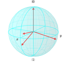
(b)

Figure 2: (a) Implementation of a random ODOP by performing a randomly selected [probability $P(\lambda)$], basis-changing unitary $U(\lambda)$ before making a projective measurement of a standard observable $O$, with outcomes $o_{j}$. (b) POVM elements, represented as Bloch vectors, for the tetrahedron measurement, an example of a POVM that cannot be implemented as a random ODOP, because the POVM elements cannot be sorted into sets of equally weighted orthogonal projectors.

Identifying other subsets of POVMs as “basic” might yield other interesting lines of inquiry. For example, when doing tomography on ensembles of atoms, weak collective measurements might be compared with nonadaptive separable projective measurements SmiSilDeu2006 ; CooRioDeu2014 .

II.2 Efficacy

Users of tomographic schemes are arguably less interested in the novelty of a particular approach than they are in its performance. There is a variety of performance metrics available for state estimates, some of which have operational interpretations relevant for particular applications. Given that we have no particular application in mind, we adopt a reasonable figure of merit, Haar-invariant average fidelity, which fortuitously is the figure of merit already used to analyze the scheme we consider in Sec. IV. This is the fidelity, $f\big{(}\rho,\hat{\rho}(\chi)\big{)}$, of the estimated state $\hat{\rho}(\chi)$ with the true state $\rho$, averaged over possible measurement records $\chi$ and further averaged over the unitarily invariant (maximally uninformed) prior distribution over pure true states. For the case of discrete measurement outcomes, this quantity is written as

$$F\big{(}\hat{\rho},E\big{)} \mathrel{\mathop{:}}=\int d\rho\sum_{\chi}\Pr(\chi|\rho)f\big{(}\rho,\hat{\rho}(\chi)\big{)}\,.$$ (6)

An obvious problem with this figure of merit is its dependence on the estimator $\hat{\rho}$. We want to compare measurement schemes directly, not measurement–estimator pairs. To remove this dependence we should calculate the average fidelity with the optimal estimator for each measurement, expressed as

$$F(E) \mathrel{\mathop{:}}=\max_{\hat{\rho}}F\big{(}\hat{\rho},E\big{)}\,.$$ (7)

To avoid straw-man arguments, it is also important to compare the performance of a particular tomographic protocol to the optimal protocol, or at least the best known protocol. Both proposals we review in this paper are nonadaptive measurements on each copy of the system individually. Since there are practical reasons for restricting to this class of measurements, we compare to the optimal protocol subject to this constraint.

This brings up an interesting point that can be made before looking at any of the details of the weak-measurement proposals. For our chosen figure of merit, the optimal individual nonadaptive measurement is a random ODOP (specifically the Haar-invariant measurement, which samples a measurement basis from a uniform distribution of bases according to the Haar measure). Therefore, weak-measurement schemes cannot hope to do better than random ODOPs, and even if they are able to attain optimal performance, weak measurements are clearly not an essential ingredient for attaining that performance.

II.3 Foundational significance

Many proposals for weak-measurement tomography are motivated not by efficacy, but rather by a desire to address some foundational aspect of quantum mechanics. This desire offers an explanation for the attention these proposals receive in spite of the disappointing performance we find when they are compared to random ODOPs.

There are two prominent claims of foundational significance. The first is that a measurement provides an operational interpretation of wavefunction amplitudes more satisfying than traditional interpretations. This is the motivation behind the direct state tomography of Sec. III, where the measurement allegedly yields expectation values directly proportional to wavefunction amplitudes rather than their squares.

The second claim is that weak measurement finds a clever way to get around the uncertainty–disturbance relations in quantum mechanics. The intuition behind using weak measurements in this pursuit is that, since weak measurements minimally disturb the system being probed, they might leave the system available for further use; the information obtained from a subsequent measurement, together with the information acquired from the preceding weak measurements, might be more information in total than can be obtained with traditional approaches. Of course, generalized measurement theory sets limits on the amount of information that can be extracted from a system, suggesting that such a foundational claim is unfounded. We more fully evaluate this claim in Sec. IV.

III Direct state tomography

In LunSutPat2011 and LunBab2012 Lundeen et al. propose a measurement technique designed to provide an operational interpretation of wavefunction amplitudes. They make various claims about the measurement, including its ability to make “the real and imaginary components of the wavefunction appear directly” on their measurement device, the absence of a requirement for global reconstruction since “states can be determined locally, point by point,” and the potential to “characterize quantum states in situ …without disturbing the process in which they feature.” The protocol is thus often characterized as direct state tomography (DST).

To evaluate these claims, we apply the principles discussed in Sec. II.  Lundeen et al. have outlined procedures for both pure and mixed states. We focus on the pure-state problem for simplicity, although much of what we identify is directly applicable to mixed-state DST. To construct the POVM, we need to describe the measurement in detail. The original proposal for DST of Lundeen et al. calls for a continuous meter for performing the weak measurements. As shown by Maccone and Rusconi MacRus2014 , the continuous meter can be replaced by a qubit meter prepared in the positive $\sigma_{x}$ eigenstate $\left|{+}\right\rangle$, a replacement we adopt to simplify the analysis. Since wavefunction amplitudes are basis-dependent quantities, it is necessary to specify the basis in which we want to reconstruct the wavefunction. We call this the reconstruction basis and denote it by $\left\{\left|{n}\right\rangle\right\}_{0\leq n<d}$, where $d$ is the dimension of the system we are reconstructing.

The meter is coupled to the system via one of a collection of interaction unitaries $\left\{U_{\varphi,n}\right\}_{0\leq n<d}$, where

$$U_{\varphi,n} \mathrel{\mathop{:}}=e^{-i\varphi\left|{n}\middle\rangle\middle\langle{n}\right|\otimes\sigma_{z}}\,.$$ (8)

The strength of the interaction is parametrized by $\varphi$. A weak interaction, i.e., one for which $|\varphi|\ll 1$, followed by measuring either $\sigma_{y}$ or $\sigma_{z}$ on the meter, effects a weak measurement of the system. In addition, after the interaction, there is a strong (projective) measurement directly on the system in the conjugate basis $\left\{\left|{c_{j}}\right\rangle\right\}_{0\leq j<d}$, which is defined by

$$\left\langle{n}\middle|{c_{j}}\right\rangle=\omega^{nj}/\sqrt{d}\;,\qquad\omega\mathrel{\mathop{:}}=e^{2\pi i/d}\,.$$ (9)

The protocol for DST of Lundeen et al., motivated by thinking in terms of weak values, discards all the data except for the case when the outcome of the projective measurement is $c_{0}$. This protocol is depicted as a quantum circuit in Fig. 3.

Figure 3: Quantum circuit depicting direct state tomography. The meter is coupled to the system via one of a family of unitaries, $\left\{U_{\varphi,n}\right\}_{0\leq n<d}$, each of which corresponds to a reconstruction-basis element. The meter is then measured in either the $y$ or $z$ basis to obtain information about either the real or imaginary part of the wavefunction amplitude of the selected reconstruction-basis element. This procedure is postselected on obtaining the $c_{0}$ outcome from the measurement of the system in the conjugate basis. While the postselection is often described as producing an effect on the meter, the circuit makes clear that the measurements can be performed in either order, so it is equally valid to say the measurement of the meter produces an effect on the system.

For each $n$, the expectation values of $\sigma_{y}$ and $\sigma_{z}$, conditioned on obtaining the outcome $c_{0}$ from the projective measurement, are given by

$$\begin{split}\left.{\left\langle{\sigma_{y}}\right\rangle}\right|_{n,c_{0}}&=\frac{2\sin\varphi}{d\,\Pr\!\big{(}c_{0}|U_{n,\varphi},\psi\big{)}}\operatorname{Re}(\psi_{n}\Upsilon^{*})\\ &\qquad+\frac{\sin 2\varphi-2\sin\varphi}{d\,\Pr\!\big{(}c_{0}|U_{n,\varphi},\psi\big{)}}|\psi_{n}|^{2}\,,\end{split}$$ (10)

$$\left.{\left\langle{\sigma_{z}}\right\rangle}\right|_{n,c_{0}} =\frac{2\sin\varphi}{d\,\Pr\!\big{(}c_{0}|U_{n,\varphi},\psi\big{)}}\operatorname{Im}(\psi_{n}\Upsilon^{*})\,,$$ (11)

where $\psi_{n}\mathrel{\mathop{:}}=\left\langle{n}\middle|{\psi}\right\rangle$. The probability for obtaining outcome $c_{0}$ is

$$\begin{split}&\Pr\!\big{(}c_{0}|U_{n,\varphi},\psi\big{)}\\ &\;=\frac{1}{d}\Big{(}|\Upsilon|^{2}+2(\cos\varphi-1)\big{[}\operatorname{Re}(\psi_{n}\Upsilon^{*})-|\psi_{n}|^{2}\big{]}\Big{)}\,,\end{split}$$ (12)

and

$$\Upsilon \mathrel{\mathop{:}}=\sum_{n}\psi_{n}\,.$$ (13)

We can always choose the unobservable global phase of $\left|{\psi}\right\rangle$ to make $\Upsilon$ real and positive. With this choice, which we adhere to going forward, $\left.{\left\langle{\sigma_{y}}\right\rangle}\right|_{n,c_{0}}$ provides information about the real part of $\psi_{n}$, and $\left.{\left\langle{\sigma_{z}}\right\rangle}\right|_{n,c_{0}}$ provides information about the imaginary part of $\psi_{n}$.

Specializing these results to weak measurements gives

$$\psi_{n} =\frac{\Upsilon}{2\varphi}\!\left(\left.{\left\langle{\sigma_{y}}\right\rangle}\right|_{c_{0},n}+i\!\left.{\left\langle{\sigma_{z}}\right\rangle}\right|_{c_{0},n}\right)+\mathcal{O}(\varphi^{2})\,.$$ (14)

This is a remarkably simple formula for estimating the state $\left|{\psi}\right\rangle$! There is, however, an important detail that should temper our enthusiasm. Contrary to the claim in LunBab2012 , this formula does not allow one to reconstruct the wavefunction point-by-point (amplitude-by-amplitude in this case of a finite-dimensional system), because one has no idea of the value of the “normalization constant” $\Upsilon$ until all the wavefunction amplitudes have been measured. This means that while ratios of wavefunction amplitudes can be reconstructed point-by-point, reconstructing the amplitudes themselves requires a global reconstruction. Admittedly, this reconstruction is simpler than commonly used linear-inversion techniques, but it comes at the price of an inherent bias in the estimator, arising from the weak-measurement approximation, as was discussed in MacRus2014 .

The scheme as it currently stands relies heavily on postselection, a procedure that often discards relevant data. To determine what information is being discarded and whether it is useful, we consider the measurement statistics of $\sigma_{y}$ and $\sigma_{z}$ conditioned on an arbitrary outcome $c_{m}$ of the strong measurement. To do that, we first introduce a unitary operator $Z$, diagonal in the reconstruction basis, which cyclically permutes conjugate-basis elements and puts phases on reconstruction-basis elements:

$$Z\left|{c_{j}}\right\rangle=\left|{c_{j+1}}\right\rangle\,,\qquad Z\left|{n}\right\rangle=\omega^{n}\left|{n}\right\rangle\,.$$ (15)

As is illustrated in Fig. 4, postselecting on outcome $c_{m}$ with input state $\left|{\psi}\right\rangle$ is equivalent to postselecting on $c_{0}$ with input state $Z^{-m}\left|{\psi}\right\rangle=\sum_{n}\omega^{-mn}\psi_{n}\left|{n}\right\rangle$.

(a)

(b)

Figure 4: (a) Postselection on outcome $c_{m}$, achieved by postselecting on $c_{0}$ after cyclic permutation of the conjugate basis by application of the unitary $Z^{-m}$. (b) Since $Z$ commutes with $U_{\varphi,n}$, (a) is identical to postselecting on $c_{0}$ with input state $Z^{-m}\left|{\psi}\right\rangle$.

Armed with this realization, we can write reconstruction formulae for all postselection outcomes,

$$\psi_{n}=\omega^{mn}\frac{\Upsilon}{2\varphi}\!\left(\left.{\left\langle{\sigma_{y}}\right\rangle}\right|_{c_{m},n}+i\!\left.{\left\langle{\sigma_{z}}\right\rangle}\right|_{c_{m},n}\right)+\mathcal{O}(\varphi^{2})\,.$$ (16)

This makes it obvious that all the measurement outcomes in the conjugate basis give “direct” readings of the wavefunction in the weak-measurement limit. Postselection in this case is not only harmful to the performance of the estimator, it is not even necessary for the interpretational claims of DST. Henceforth, we drop the postselection and include all the data produced by the strong measurement.

The uselessness of postselection is not a byproduct of the use of a qubit meter. In the continuous-meter case, the conditional expectation values in the weak-measurement limit are given as weak values

$$\left.{\left\langle{\left|{x}\middle\rangle\middle\langle{x}\right|}\right\rangle}\right|_{p} =\frac{\left\langle{p}\middle|{x}\right\rangle\left\langle{x}\middle|{\psi}\right\rangle}{\left\langle{p}\middle|{\psi}\right\rangle}\,.$$ (17)

Weak-value-motivated DST postselects on meter outcome $p=0$ to hold the amplitude $\left\langle{p}\middle|{x}\right\rangle$ constant and thus make the expectation value proportional to the wavefunction $\left\langle{x}\middle|{\psi}\right\rangle$. Since $\left\langle{p}\middle|{x}\right\rangle$ is only a phase, however, it is again obvious that postselecting on any value of $p$ gives a “direct” reconstruction of a rephased wavefunction. Shi et al. Shi2015 have developed a variation on Lundeen’s protocol that requires measuring weak values of only one meter observable. This is made possible by keeping data that is discarded in the original postselection process.

We now consider whether the weak measurements in DST contribute anything new to tomography. It is already clear from Eqs. (10) and (11) that for this protocol to provide data that is proportional to amplitudes in the reconstruction basis, the weakness of the interaction is only important for the measurement of $\sigma_{y}$. We are after something deeper than this, however, and to get at it, we change perspective on the protocol of Fig. 3, asking not how postselection on the result of the strong measurement affects the measurement of $\sigma_{y}$ or $\sigma_{z}$, but rather how those measurements change the description of the strong measurement. As is discussed in Fig. 3, this puts the protocol on a footing that resembles that of the random ODOPs in Fig. 2(a).

The measurement of $\sigma_{z}$, which provides the imaginary-part information, is trivial to analyze, because the analysis can be reduced to drawing more circuits. In Fig. 5(a), the interaction unitary is written in terms of system unitaries $U_{n,\pm}\mathrel{\mathop{:}}=e^{\mp i\varphi\otimes\left|{n}\middle\rangle\middle\langle{n}\right|}$ that are controlled in the $z$-basis of the qubit. The $\sigma_{z}$ measurement on the meter commutes with the interaction unitary, so using the principle of deferred measurement, we can move this measurement through the controls, which become classical controls that use the results of the measurement. The resulting circuit, depicted in Fig. 5(b), shows that the imaginary part of each wavefunction amplitude can be measured by adding a phase to that amplitude, with the sign of the phase shift determined by a coin flip. This is a particular example of the random ODOP described by Fig. 2(a). We conclude that weak measurements are not an essential ingredient for determining the imaginary parts of the wavefunction amplitudes.

(a)

(b)

Figure 5: (a) The imaginary-part measurement in a circuit where the interaction unitary is written in terms of system unitaries $U_{n,\pm}\mathrel{\mathop{:}}=e^{\mp i\varphi\left|{n}\middle\rangle\middle\langle{n}\right|}$ controlled in the $z$-basis. This circuit is equivalent to that of Fig. 3 when $\sigma_{z}$ is measured on the meter; the result of the measurement reveals the sign of interaction, i.e., which of the unitaries $U_{n,\pm}$ was applied to the system. (b) The coherent controls can be turned into classical controls by moving the measurement before the controls. The result is a particular instance of the random ODOP depicted in Fig. 2(a).

Measuring the real parts is more interesting, since the $\sigma_{y}$ measurement does not commute with the interaction unitary. We proceed by finding the Kraus operators that describe the post-measurement state of the system. The strong, projective measurement in the conjugate basis has Kraus operators $K_{m}=\left|{c_{m}}\middle\rangle\middle\langle{c_{m}}\right|$, whereas the unitary interaction $U_{\varphi,n}$, followed by the measurement of $\sigma_{y}$ with outcome $\pm$, has (Hermitian) Kraus operator

$$\begin{split}K_{\pm}^{(y,n)}&\mathrel{\mathop{:}}=\left\langle{\pm y}\right|U_{\varphi,n}\left|{+}\right\rangle\\ &=\frac{1}{\sqrt{2}}\left(\mathds{1}+\big{(}\sqrt{2}s_{\pm}-1\big{)}\left|{n}\middle\rangle\middle\langle{n}\right|\right)\,,\\ s_{\pm}&\mathrel{\mathop{:}}=\pm\sin(\varphi\pm\pi/4)\,,\end{split}$$ (18)

where the eigenstates of $\sigma_{y}$ are $\left|{\pm y}\right\rangle\mathrel{\mathop{:}}=\big{(}e^{\mp i\pi/4}\left|{0}\right\rangle+e^{\pm i\pi/4}\left|{1}\right\rangle\big{)}/\sqrt{2}$. The composite Kraus operators, $K_{\pm,m}^{(y,n)}=K_{m}K_{\pm}^{(y,n)}$, yield POVM elements $E_{\pm,m}^{(y,n)}\mathrel{\mathop{:}}=K_{\pm,m}^{(y,n)\dagger}K_{\pm,m}^{(y,n)}=K_{\pm}^{(y,n)}\left|{c_{m}}\middle\rangle\middle\langle{c_{m}}\right|K_{\pm}^{(y,n)}$. For each $n$, these POVM elements make up a rank-one POVM with $2d$ outcomes.

The POVM elements can productively be written as

$$E_{\pm,m}^{(y,n)} =\alpha^{(y)}_{\pm}\left|{b_{\pm,m}^{(y,n)}}\middle\rangle\middle\langle{b_{\pm,m}^{(y,n)}}\right|\,,$$ (19)

$$\begin{split}\left|{b_{\pm,m}^{(y,n)}}\right\rangle&\mathrel{\mathop{:}}=K_{\pm}^{(y,n)}\left|{c_{m}}\right\rangle\Big{/}\sqrt{\alpha^{(y)}_{\pm}}\\ &=\left(\left|{c_{m}}\right\rangle+\big{(}\sqrt{2}s_{\pm}-1\big{)}\omega^{mn}\left|{n}\right\rangle\right)\Big{/}\sqrt{2\alpha^{(y)}_{\pm}}\,,\end{split}$$ (20)

$$\alpha^{(y)}_{\pm} \mathrel{\mathop{:}}=\frac{1}{2}\!\left(1-\frac{1}{d}+\frac{2}{d}s_{\pm}^{2}\right)\,.$$ (21)

The POVM for each $n$ does not fit into our framework of random ODOPs, but can be thought of as within a wider framework of random POVMs. Indeed, the Neumark extension Neumark1940 ; Peres1993 teaches us how to turn any rank-one POVM into an ODOP in a higher-dimensional Hilbert space, where the dimension matches the number of outcomes of the rank-one POVM.

Vallone and Dequal ValDeq2015 have proposed an augmentation of the original DST to obtain a “direct” wavefunction measurement without the need for the weak-measurement approximation. The essence of their protocol is to perform an additional $\sigma_{x}$ measurement on the meter. The statistics of this measurement allow the second-order term in $\varphi$ to be eliminated from the real-part calculation, giving a reconstruction formula that is exact for all values of $\varphi$. Of course, the claim that the original DST protocol “directly” measures the wavefunction is misleading, and directness claims for Vallone and Dequal’s modifications are necessarily more misleading. Even ratios of real parts of wavefunction amplitudes no longer can be obtained by ratios of simple expectation values, since these calculations rely on both $\sigma_{x}$ and $\sigma_{y}$ expectation values for different measurement settings.

We analyze this additional meter measurement in the same way we analyzed the $\sigma_{y}$ measurement. The Kraus operators corresponding to the meter measurements are

$$K_{+}^{(x,n)} \mathrel{\mathop{:}}=\left\langle{+}\right|U_{\varphi,n}\left|{+}\right\rangle=\mathds{1}+\big{(}\cos\varphi-1\big{)}\left|{n}\middle\rangle\middle\langle{n}\right|\,,$$ (22)

$$K_{-}^{(x,n)} \mathrel{\mathop{:}}=\left\langle{-}\right|U_{\varphi,n}\left|{+}\right\rangle=\sin\varphi\left|{n}\middle\rangle\middle\langle{n}\right|\,.$$ (23)

The composite Kraus operators, $K_{\pm,m}^{(x,n)}=K_{m}K_{\pm}^{(x,n)}$, yield POVM elements $E_{\pm,m}^{(x,n)}$ that can be written as

$$E_{\pm,m}^{(x,n)} =\alpha^{(x)}_{\pm}\left|{b_{\pm,m}^{(x,n)}}\middle\rangle\middle\langle{b_{\pm,m}^{(x,n)}}\right|\,,$$ (24)

$$\begin{split}\left|{b_{+,m}^{(x,n)}}\right\rangle&\mathrel{\mathop{:}}=K_{+}^{(x,n)}\left|{c_{m}}\right\rangle\Big{/}\sqrt{\alpha^{(x)}_{+}}\\ &=\Big{(}\left|{c_{m}}\right\rangle+\big{(}\cos\varphi-1\big{)}\omega^{mn}\left|{n}\right\rangle\Big{)}\Big{/}\sqrt{\alpha^{(x)}_{+}}\,,\end{split}$$ (25)

$$\left|{b_{-,m}^{(x,n)}}\right\rangle \mathrel{\mathop{:}}=K_{-}^{(x,n)}\left|{c_{m}}\right\rangle\Big{/}\sqrt{\alpha^{(x)}_{-}}=\left|{n}\right\rangle\,,$$ (26)

$$\alpha^{(x)}_{+} \mathrel{\mathop{:}}=1-\frac{\sin^{2}\!\varphi}{d}\,,\qquad\alpha^{(x)}_{-}\mathrel{\mathop{:}}=\frac{\sin^{2}\!\varphi}{d}\,.$$ (27)

It is useful to ponder the form of the POVM elements for the $\sigma_{y}$ and $\sigma_{x}$ measurements of the DST protocols. For the original DST protocol of Fig. 3, without postselection, the only equatorial measurement on the meter is of $\sigma_{y}$; the corresponding POVM elements, given by Eq. (19), are nearly measurements in the conjugate basis, except that the $n$-component of the conjugate basis vector is changed in magnitude by an amount that depends on the result of the $\sigma_{y}$ measurement. For the augmented DST protocol of Vallone and Dequal, the additional POVM elements (24), which come from the measurement of $\sigma_{x}$ on the meter, are quite different depending on the result of the $\sigma_{x}$ measurement. For the result $+$, the POVM element is similar to the POVM elements for the measurement of $\sigma_{y}$, but with a different modification of the $n$-component of the conjugate vector. For the result $-$, the POVM element is simply a measurement in the reconstruction basis; as we see below, the addition of the measurement in the reconstruction basis has a profound effect on the performance of the augmented DST protocol outside the region of weak measurements, an effect unanticipated by the weak-value motivation.

Although claims regarding the efficacy of DST are rather nebulous, we consider the negative impact of the weak-measurement limit on tomographic performance. In doing so, we assume for simplicity that the system is a qubit, in some unknown pure state that is specified by polar and azimuthal Bloch-sphere angles, $\theta$ and $\phi$. In this case we assume that the reconstruction basis is the eigenbasis of $\sigma_{z}$; the conjugate basis is the eigenbasis of $\sigma_{x}$.

The method we use to evaluate the effect of variations in $\varphi$ is taken from the work of de Burgh et al. deBurgh2008 , which uses the Cramér–Rao bound (CRB) to establish an asymptotic (in number of copies) form of the average fidelity.

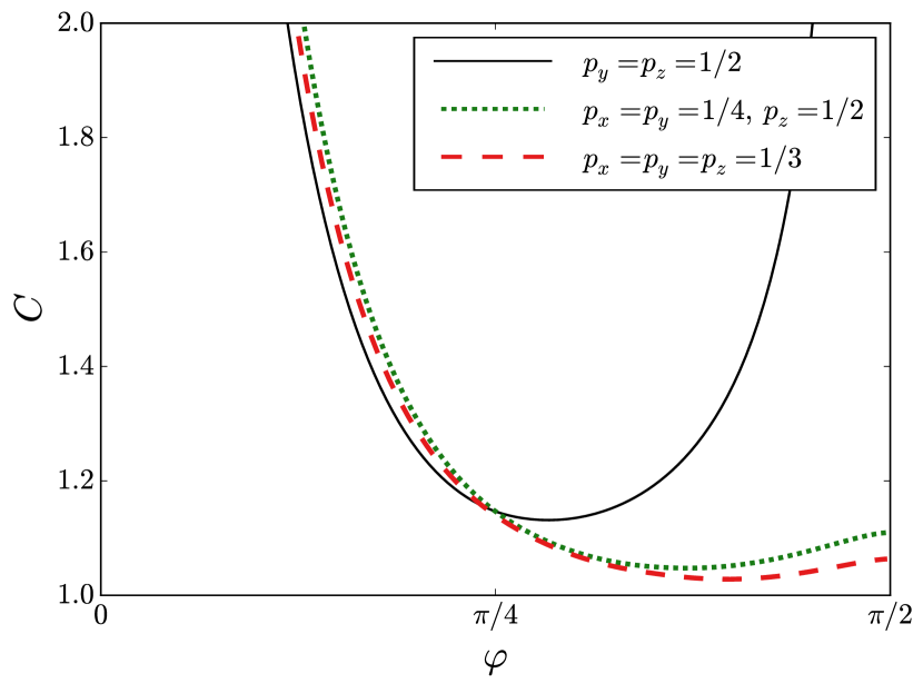
Figure 6: (Color online) CRB $C(\varphi)$ of Eq. (29) for original DST (solid black) and augmented DST (dotted green for probability $1/4$ for $\sigma_{x}$ and $\sigma_{y}$ measurements and $1/2$ probability for a $\sigma_{z}$ measurement; dashed red for equal probabilities for all three measurements). As the plot makes clear, the optimal values for $\varphi$ are far from the weak-measurement limit. Values of $\varphi$ for which $\varphi^{2}\simeq 0$ give exceptionally large CRBs, confirming the intuition that weak measurements learn about the true state very slowly. The CRB for original DST also grows without bound as $\varphi$ approaches $\pi/2$, since that measurement strength leads to degenerate Kraus operators and a POVM that, not informationally complete, consists only of projectors onto $\sigma_{x}$ and $\sigma_{y}$ eigenstates of the system. The CRB remains finite when the meter measurements are augmented with $\sigma_{x}$, since the resultant POVM at $\varphi=\pi/2$ then includes $\sigma_{z}$ projectors on the system [i.e., projectors in the reconstructions basis; see Eq. (26)], giving an informationally complete overall POVM.

In analyzing the two DST protocols, original and augmented, we assume that the two values of $n$ are chosen randomly with probability $1/2$. For the original protocol, we choose the $\sigma_{z}$ and $\sigma_{y}$ measurements with probability $1/2$. For the augmented protocol, we make one of two choices: equal probabilities for the $\sigma_{x}$, $\sigma_{y}$, and $\sigma_{z}$ measurements or probabilities of $1/2$ for the $\sigma_{z}$ measurement and $1/4$ for the $\sigma_{x}$ and $\sigma_{y}$ measurements. Formally, these assumed probabilities scale the POVM elements when all of them are combined into a single overall POVM.

The asymptotic form involves the Fisher informations, $J_{\theta}$ and $J_{\phi}$, for the two Bloch-sphere state parameters, calculated from the statistics of whatever measurement we are making on the qubit. The CRB already assumes the use of an optimal estimator. When the number of copies, $N$, is large, the average fidelity takes the simple form

$$F(\varphi) \simeq 1-\frac{1}{N}C(\varphi)\,,$$ (28)

$$\begin{split}C(\varphi)&=\int_{0}^{\pi}d\theta\,\sin\theta\\ &\quad\times\int_{0}^{2\pi}d\phi\,\frac{1}{4}\!\!\left(\frac{1}{J_{\theta}(\theta,\phi,\varphi)}+\frac{\sin^{2}\theta}{J_{\phi}(\theta,\phi,\varphi)}\!\right)\,.\end{split}$$ (29)

Though we have derived analytic expressions for the Fisher informations, it is more illuminating to plot the CRB $C(\varphi)$, obtained by numerical integration (see Fig. 6). For original DST, the optimal value of $\varphi$ is just beyond $\pi/4$, invalidating all qualities of “directness” that come from assuming $\varphi\ll 1$. For the augmented DST of Vallone and Dequal, the optimal value of $\varphi$ moves toward $\pi/2$, even further outside the region of weak measurements. In both cases, $C(\varphi)$ blows up at $\varphi=0$; for weak measurements, $C(\varphi)$ is so large that the information gain is glacial.

We visualize this asymptotic behavior by estimating the average fidelity over pure states as a function of $N$ using the sequential Monte Carlo technique smc_foot , for various protocols and values of $\varphi$. Figure 7 plots these results and shows how the average fidelity, for the optimal value of $\varphi$, approaches the asymptotic form (28) as $N$ increases. We note that the estimator used in these simulations is the estimator optimized for average fidelity discussed in BagBalGil2006 . If we were to use the reconstruction formula proposed by Lundeen et al., the performance would be worse.

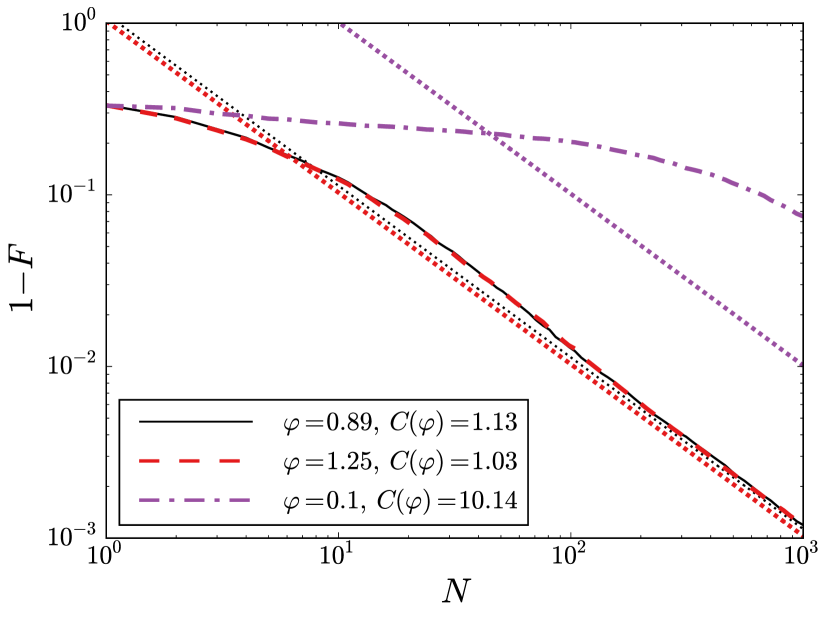
Figure 7: (Color online) Average infidelity $1-F$ as a function of the number $N$ of system copies for three measurements. The dashed red curve is for augmented DST with equal probabilities for the three meter measurements; the value $\varphi=1.25$ is close to the optimal value from Fig. 6. The other two curves are for original DST: the solid black curve is for $\varphi=0.89$, which is close to optimal (this curve nearly coincides with the dashed red curve for augmented DST); the dashed-dotted purple curve is for a small value $\varphi=0.1$, where the weak-measurement approximation is reasonable. The three dotted curves give the corresponding asymptotic behavior $C(\varphi)/N$. The two weak-measurement curves illustrate the glacial information acquisition when weak measurements are used; the dashed-dotted curve hasn’t begun to approach the dotted asymptotic form for $N=10^{3}$.

Our conclusions are the following. First, postselection contributes nothing to DST. Its use comes from attention to weak values, but postselection is actually a negative for tomography because it discards data that are just as cogent as the data that are retained in the weak-value scenario. Second, weak measurements in this context add very little to a tomographic framework based on random ODOPs. Finally, the “direct” in DST is a misnomer misnomer because the protocol does not provide point-by-point reconstruction of the wavefunction.

The inability to provide point-by-point reconstruction is a symptom of a general difficulty. Any procedure, classical or quantum, for detecting a complex amplitude when only absolute squares of amplitudes are measurable involves interference between two amplitudes, say, $A$ and $B$, so that some observed quantity involves a product of two amplitudes, say, ${\rm Re}(A^{*}B)$. If one regards $A$ as “known” and chooses it to be real, then ${\rm Re}(B)$ can be said to be observed directly. This is the way amplitudes and phases of classical fields are determined using interferometry and square-law detectors.

Of course, quantum amplitudes are not classical fields. One loses the ability to say that one amplitude is known and objective, with the other to be determined relative to the known amplitude. Indeed, if one starts from the tomographic premise that nothing is known and everything is to be estimated from measurement statistics, then $A$ cannot be regarded as “known.” DST fits into this description, with the sum of amplitudes, $\Upsilon$ of Eq. (13), made real by convention, playing the role of $A$. The achievement of DST is that this single quantity is the only “known” quantity needed to construct all the amplitudes $\psi_{n}$ from measurement statistics. Single quantity or not, however, $\Upsilon$ must be determined from the entire tomographic procedure before any of the amplitudes $\psi_{n}$ can be estimated.

IV Weak-measurement tomography

The second scheme we consider is a proposal for qubit tomography by Das and Arvind DasArv2014 . This protocol was advertised as opening up “new ways of extracting information from quantum ensembles” and outperforming, in terms of fidelity, tomography performed using projective measurements on the system. The optimality claim cannot be true, of course, since a random ODOP based on the Haar invariant measure for selecting the ODOP basis is optimal when average fidelity is the figure of merit, but the novelty of the information extraction remains to be evaluated.

Figure 8: Quantum circuit depicting the weak-measurement tomography protocol of Das and Arvind. Two identical meters are used as ancillas to perform the weak $z$ and $x$ measurements. The circuit makes clear that there is nothing important in the order the measurements are performed after the interactions have taken place, so we consider the protocol as a single ancilla-coupled measurement.

The weak measurements in this proposal are measurements of Pauli components of the qubit. These measurements are performed by coupling the qubit system via an interaction unitary,

$$U^{(j)}=e^{-i\sigma_{j}\otimes P}\,,$$ (30)

to a continuous meter, which has position $Q$ and momentum $P$ and is prepared in the Gaussian state

$$\left|{\phi}\right\rangle=\sqrt[4]{\frac{\epsilon}{2\pi}}\int_{-\infty}^{\infty}dq\,e^{-\epsilon q^{2}/4}\left|{q}\right\rangle\,.$$ (31)

The position of the meter is measured to complete the weak measurement. The weakness of the measurement is parametrized by $\epsilon=1/\Delta q^{2}$.

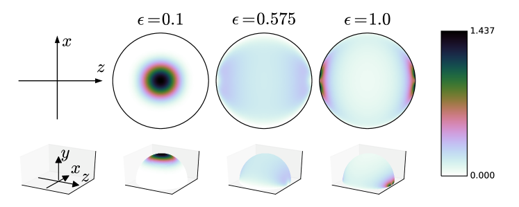
Figure 9: (Color online) Effective distributions over measurement bases visualized as distributions over the positive-$y$ Bloch hemisphere. Very weak measurements of $z$ and $x$ (e.g., $\epsilon=0.1$) don’t perturb the final $y$ measurement very much, so the distribution of bases is concentrated about the $y$ axis. Very strong measurements (e.g., $\epsilon=1$) end up extracting most of the information in the first $z$ measurement, so the distribution becomes concentrated around the $z$ axis. The optimal measurement ($\epsilon\simeq 0.575$) has an effective distribution that is nearly uniform.

The Das-Arvind protocol involves weakly measuring the $z$ and $x$ Pauli components and then performing a projective measurement of $\sigma_{y}$. We depict this protocol as a circuit in Fig. 8. Das and Arvind view this protocol as providing more information than is available from the projective $\sigma_{y}$ measurement because the weak measurements extract a little extra information about the $z$ and $x$ Pauli components without appreciably disturbing the state of the system before it is slammed by the projective $\sigma_{y}$ measurement. Again, we turn the tables on this point of view, with its notion of a little information flowing out to the two meters, to a perspective akin to that of the random ODOP of Fig. 2(a). We ask how the weak measurements modify the description of the final projective measurement. For this purpose, we again need Kraus operators to calculate the POVM of the overall measurement.

The Kraus operators for the projective measurement are $K^{(y)}_{\pm}=\left|{\pm y}\middle\rangle\middle\langle{\pm y}\right|$, and the (Hermitian) Kraus operator for a weak measurement with outcome $q$ on the meter is

$$\begin{split}K^{(j)}(q)&\mathrel{\mathop{:}}=\left\langle{q}\right|\,U^{(j)}\left|{\phi}\right\rangle\sqrt{dq}\\ &=\sqrt[4]{\frac{\epsilon}{2\pi}}\exp\!\left(-\frac{\epsilon(q^{2}+1)}{4}\right)\\ &\quad\times\Big{(}\mathds{1}\cosh(\epsilon q/2)+\sigma_{j}\sinh(\epsilon q/2)\Big{)}\sqrt{dq}\,.\end{split}$$ (32)

The Kraus operators for the whole measurement procedure are $K_{\pm}(q_{1},q_{2})\mathrel{\mathop{:}}=K^{(y)}_{\pm}K^{(x)}(q_{2})K^{(z)}(q_{1})$. From these come the infinitesimal POVM elements for outcomes $q_{1}$, $q_{2}$, and $\pm$:

$$\begin{split}d&E_{\pm}(q_{1},q_{2})\\ &\,\mathrel{\mathop{:}}=K^{\dagger}_{\pm}(q_{1},q_{2})K_{\pm}(q_{1},q_{2})\\ &\,=K^{(z)}(q_{1})K^{(x)}(q_{2})\left|{\pm y}\middle\rangle\middle\langle{\pm y}\right|K^{(x)}(q_{2})K^{(z)}(q_{1})\,.\end{split}$$ (33)

These POVM elements are clearly rank-one.

Using the Pauli algebra, we can bring the POVM elements into the explicit form,

$$\begin{split}dE_{\pm}(q_{1},q_{2})&=K^{\dagger}_{\pm}(q_{1},q_{2})K_{\pm}(q_{1},q_{2})\\ &=dq_{1}\,dq_{2}\,G(q_{1},q_{2})\frac{1}{2}(\mathds{1}+\hat{\mathbf{n}}_{\pm}(q_{1},q_{2})\cdot\boldsymbol{\sigma})\,,\end{split}$$ (34)

where we have introduced a probability density and unit vectors,

$$\begin{split}G(q_{1},q_{2})&\mathrel{\mathop{:}}=\frac{\epsilon}{2\pi}\exp\!\left(-\frac{\epsilon(q_{1}^{2}+q_{2}^{2}+2)}{2}\right)\\ &\qquad\times\cosh\epsilon q_{1}\cosh\epsilon q_{2}\,,\end{split}$$ (35)

$$\hat{\mathbf{n}}_{\pm}(q_{1},q_{2}) \mathrel{\mathop{:}}=\frac{\hat{\mathbf{x}}\sinh\epsilon q_{2}\pm\hat{\mathbf{y}}+\hat{\mathbf{z}}\sinh\epsilon q_{1}\cosh\epsilon q_{2}}{\cosh\epsilon q_{1}\cosh\epsilon q_{2}}\,.$$ (36)

We note that $G(q_{1},q_{2})=G(-q_{1},-q_{2})$ and $\hat{\mathbf{n}}_{\pm}(q_{1},q_{2})=-\hat{\mathbf{n}}_{\mp}(-q_{1},-q_{2})$. This means that the overall POVM is made up of a convex combination of equally weighted pairs of orthogonal projectors and is therefore a random ODOP. From this perspective, the weak measurements are a mechanism for generating a particular distribution from which different projective measurements are sampled; i.e., they are a particular way of generating a distribution $P(\lambda)$ in Fig. 2. Several of these distributions are plotted in Fig. 9.

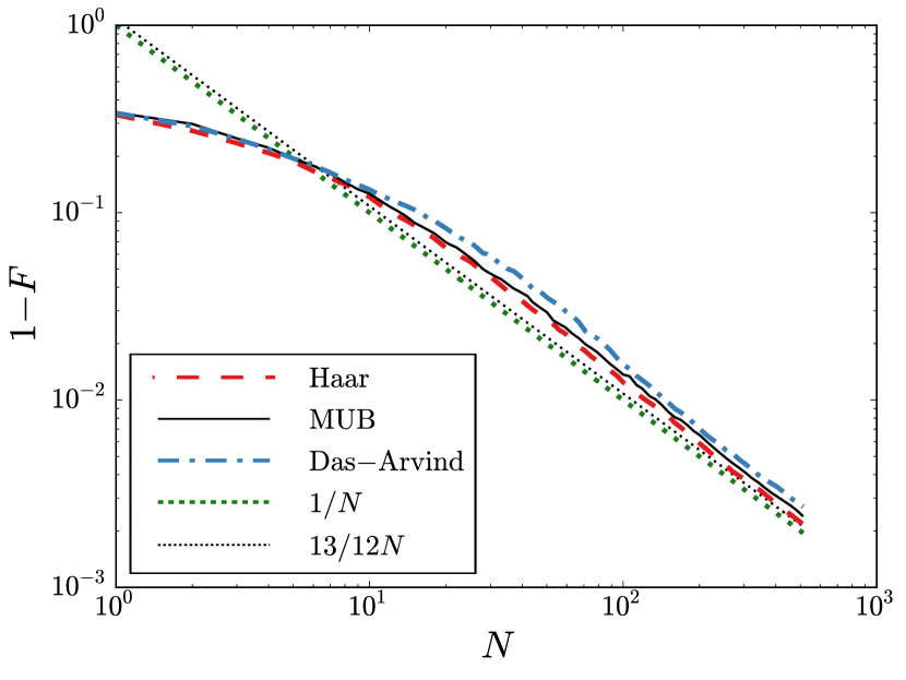
Figure 10: (Color online) Average infidelity $1-F$ as a function of the number $N$ of system copies for three measurements: Das and Arvind’s measurement protocol (dotted-dashed blue) with $\epsilon=0.575$; MUB consisting of Pauli $\sigma_{x}$, $\sigma_{y}$, and $\sigma_{z}$ measurements (solid black); random ODOP consisting of projective measurements sampled from the Haar-uniform distribution (dashed red). The dotted lines, $1/N$ and $13/12N$, are the CRBs defined by Eq. (29) for the optimal generalized tomographic protocol and MUB measurements, respectively.

It is interesting to note that the value of $\epsilon$ that Das and Arvind identified as optimal (about $0.575$) produces a distribution that is nearly uniform over the Bloch sphere. This matches our intuition when thinking of the measurement as a random ODOP, since the optimal random ODOP samples from the uniform distribution

To visualize the performance of this protocol, we again use sequential Monte Carlo simulations of the average fidelity. Das and Arvind compare their protocol to a measurement of $\sigma_{x}$, $\sigma_{y}$, and $\sigma_{z}$, whose eigenstates are mutually unbiased bases (MUB). In Fig. 10, we compare Das and Arvind’s protocol for $\epsilon=0.575$ to a MUB measurement and to the optimal projective-measurement-based tomography scheme, i.e., the Haar-uniform random ODOP.

We don’t discuss the process of binning the position-measurement results that Das and Arvind engage in, since such a process produces a rank-2 POVM that is equivalent to sampling from a discrete distribution over projective measurements and then adding noise, a practice that necessarily degrades tomographic performance.

We conclude that the protocol does not offer anything beyond that offered by random ODOPs and that its claim of extracting information about the system without disturbance is not supported by our analysis. In particular, when operated optimally, it is essentially the same as the strong projective measurements of a Haar-uniform random ODOP. It is true that the presence of the $z$ and $x$ measurements provides more information than a projective $y$ measurement by itself, but this is not because the $z$ and $x$ measurements extract information without disturbing the system.

V Summary and conclusion

Our analysis of weak-measurement tomographic schemes gives us guidance for future forays into tomography.

POVMs contain the necessary and sufficient information for comparing the performance of tomographic techniques. Specific realizations of a POVM might provide pleasing narratives, but these narratives are irrelevant for calculating figures of merit. Optimal POVMs for many figures of merit and technical limitations are known. A new tomographic proposal should identify restrictions on the set of available POVMs that come about from practical considerations and compare itself to the best known POVM in that set. The question of the optimality of Das and Arvind’s tomographic scheme is easily answered by identifying what POVMs arise from “projective measurement-based tomography” and realizing these POVMs are optimal even in the generalized nonadaptive, individual-measurement scenario.

Claims about novel properties of a state-reconstruction technique should be evaluated as a comparison with a motivated restriction on the set of POVMs. The false dichotomy between “tomographic methods” and whatever new method is being proposed obfuscates that all new methods implement a POVM and that reconstructing a state from POVM statistics is nothing but tomography. Our analysis shows that even the relatively bland and conceptually simple set of random ODOPs captures most of the behavior exhibited by more exotic protocols.

It is appropriate to move beyond the minimal, platform-independent POVM description when considering ease of implementation or when trying to provide a helpful conceptual framework. Nonetheless, a pleasing conceptual framework should not be confused with an optimal experimental arrangement. If the experimental setup described by Lundeen et al. happens to be the easiest to implement in one’s lab, the state should still be reconstructed using techniques developed in the general POVM setting rather than the perturbative reconstruction formula presented in work on DST, regardless of how attractive one finds the wavefunction-amplitude analogy.

- (1) G. M. D’Ariano, Universal quantum observables, Physics Letters A 300, 1 (2002).
- (2) S. Massar and S. Popescu, Optimal extraction of information from finite quantum ensembles, Physical Review Letters 74, 1259 (1995).
- (3) M. A. Nielsen and I. L. Chuang, Quantum Computation and Quantum Information, (Cambridge University Press, 2010).
- (4) A. S. Holevo, Probabilistic and Statistical Aspects of Quantum Theory, (North Holland, Amsterdam, 1982).
- (5) Z. Hradil, Quantum-state estimation, Physical Review A 55, R1561(R) (1997).
- (6) E. Bagan, M. A. Ballester, R. D. Gill, A. Monras, and R. Munoz-Tapia, Optimal full estimation of qubit mixed states, Physical Review A 73, 032301 (2006).
- (7) R. Blume-Kohout, Optimal, reliable estimation of quantum states, New Journal of Physics, 12, 043034 (2010).
- (8) D. Gross, Y.-K. Liu, S. T. Flammia, S. Becker, and J. Eisert, Quantum state tomography via compressed sensing, Physical Review Letters 105, 150401 (2010).
- (9) A. Barchielli, L. Lanz, and G. M. Prosperi, A model for the macroscopic description and continual observations in quantum mechanics, Il Nuovo Cimento B 72, 79 (1982).
- (10) C. M. Caves and G. J. Milburn, Quantum-mechanical model for continuous position measurements, Physical Review A 36, 5543 (1987).
- (11) G. M. D’Ariano and H. P. Yuen, Impossibility of measuring the wave function of a single quantum system, Physical Review Letters 76, 2832 (1996).
- (12) C. A. Fuchs and K. Jacobs, Information-tradeoff relations for finite-strength quantum measurements, Physical Review A 63, 062305 (2001).
- (13) O. Oreshkov and T. A. Brun, Weak measurements are universal, Physical Review Letters 95, 110409 (2005).
- (14) I. L. Chuang, N. Gershenfeld, M. G. Kubinec, and D. W. Leung, Bulk quantum computation with nuclear magnetic resonance: Theory and experiment, Proceedings of the Royal Society A: Mathematical, Physical and Engineering Sciences 454, 447 (1998).
- (15) G. A. Smith, A. Silberfarb, I. H. Deutsch, and P. S. Jessen, Efficient quantum-state estimation by continuous weak measurement and dynamical control, Physical Review Letters 97, 180403 (2006).
- (16) G. G. Gillett, R. B. Dalton, B. P. Lanyon, M. P. Almeida, M. Barbieri, G. J. Pryde, J. L. O’Brien, K. J. Resch, S. D. Bartlett, and A. G. White, Experimental feedback control of quantum systems using weak measurements, Physical Review Letters 104, 080503 (2010).
- (17) C. Sayrin, I. Dotsenko, X. Zhou, B. Peaudecerf, T. Rybarczyk, S. Gleyzes, P. Rouchon, M. Mirrahimi, H. Amini, M. Brune, J.-M. Raimond, and S. Haroche, Real-time quantum feedback prepares and stabilizes photon number states, Nature 477, 73 (2011).
- (18) R. Vijay, C. Macklin, D. H. Slichter, S. J. Weber, K. W. Murch, R. Naik, A. N. Korotkov, and I. Siddiqi, Stabilizing Rabi oscillations in a superconducting qubit using quantum feedback, Nature 490, 77 (2012).
- (19) P. Campagne-Ibarcq, E. Flurin, N. Roch, D. Darson, P. Morfin, M. Mirrahimi, M. H. Devoret, F. Mallet, and B. Huard, Persistent control of a superconducting qubit by stroboscopic measurement feedback, Physical Review X 3, 021008 (2013).
- (20) R. L. Cook, C. A. Riofrio, and I. H. Deutsch, Single-shot quantum state estimation via a continuous measurement in the strong backaction regime, Physical Review A 90, 032113 (2014).
- (21) H. M. Wiseman and G. J. Milburn, Quantum measurement and control (Cambridge University Press, 2010).
- (22) Y. Aharonov, D. Z. Albert, and L. Vaidman, How the result of a measurement of a component of the spin of a spin-1/2 particle can turn out to be 100, Physical Review Letters 60, 1351 (1988).
- (23) O. Hosten and P. Kwiat, Observation of the spin Hall effect of light via weak measurements, Science 319, 787 (2008).
- (24) G. Strübi and C. Bruder, Measuring ultrasmall time delays of light by joint weak measurements, Physical Review Letters 110, 083605 (2013).
- (25) G. C. Knee, G. A. D. Briggs, S. C. Benjamin, and E. M. Gauger, Quantum sensors based on weak-value amplification cannot overcome decoherence, Phys. Rev. A 87, 012115 (2013).
- (26) S. Tanaka and N. Yamamoto, Information amplification via postselection: A parameter-estimation perspective, Phys. Rev. A 88, 042116 (2013).
- (27) C. Ferrie and J. Combes, Weak value amplification is suboptimal for estimation and detection, Phys. Rev. Lett. 112, 040406 (2014); in particular, see the Supplementary Material.
- (28) G. C. Knee and E. M. Gauger, When amplification with weak values fails to suppress technical noise, Phys. Rev. X 4, 011032 (2014) .
- (29) J. Combes, C. Ferrie, Z. Jiang, and C. M. Caves, Quantum limits on postselected, probabilistic quantum metrology, Phys. Rev. A 89, 052117 (2014).
- (30) L. Zhang, A. Datta, and I. A. Walmsley, Precision metrology using weak measurements, arXiv:1310.5302.
- (31) J. Dressel, M. Malik, F. M. Miatto, A. N. Jordan, and R. W. Boyd, Colloquium: Understanding quantum weak values: Basics and applications, Reviews of Modern Physics 86, 307 (2014).
- (32) A. N. Jordan, J. Martinez-Rincon, and J. C. Howell, Technical advantages for weak-value amplification: When less is more, Physical Review X 4, 011031 (2014).
- (33) J. Lee and I. Tsutsui, Merit of amplification by weak measurement in view of measurement uncertainty, Quantum Studies: Mathematics and Foundations, 1, 65 (2014).
- (34) G. C. Knee, J. Combes, C. Ferrie, and E. M. Gauger, Weak-value amplification: State of play, arXiv:1410.6252
- (35) J. S. Lundeen, B. Sutherland, A. Patel, C. Stewart, and C. Bamber, Direct measurement of the quantum wavefunction, Nature 474, 188 (2011).
- (36) D. Das and Arvind, Estimation of quantum states by weak and projective measurements, Physical Review A 89, 062121 (2014).
- (37) J. S. Lundeen and C. Bamber, Procedure for direct measurement of general quantum states using weak measurement, Physical Review Letters 108, 070402 (2012).
- (38) L. Maccone and C. C. Rusconi, State estimation: A comparison between direct state measurement and tomography, Physical Review A 89, 022122 (2014).
- (39) M. A. Neumark (aka Naimark), Spectral functions of a symmetric operator, Izvestya Acad. Nauk SSSR: Ser. Mat. 4, 277 (1940).
- (40) A. Peres, Quantum Theory: Concepts and Methods (Kluwer, 1993).
- (41) G. Vallone and D. Dequal, Direct measurement of the quantum wavefunction by strong measurements, arXiv:1504.06551.
- (42) Z. Shi, M. Mirhosseini, J. Margiewicz, M. Malik, F. Rivera, Z. Zhu, and R. W. Boyd, Scan-free direct measurement of an extremely high-dimensional photonic state, Optica 2, 388–392 (2015)
- (43) M. D. de Burgh, N. K. Langford, A. C. Doherty and A. Gilchrist, Choice of measurement sets in qubit tomography, Physical Review A 78, 052122 (2008).
- (44) C. E. Granade, C. Ferrie, N. Wiebe, and D. G. Cory, Robust online Hamiltonian learning, New Journal of Physics 14, 103013 (2012).
- (45) C. Granade and C. Ferrie, QInfer: Library for Statistical Inference in Quantum Information, (2012).
- (46) The sequential Monte Carlo algorithm was detailed in granade2012 and implemented in qinfer .
- (47) In the long tradition of institutions abandoning a name in favor of initials, to divorce from some original product or purpose, we recommend the use of DST in the hope that the “direct” can be forgotten.