A new Phase Space Density for Quantum Expectations

Johannes Keller Zentrum Mathematik, Technische Universität München, Boltzmannstraße 3, 85748 Garching bei München. keller@ma.tum.de Caroline Lasser Zentrum Mathematik, Technische Universität München, Boltzmannstraße 3, 85748 Garching bei München. classer@ma.tum.de  and  Tomoki Ohsawa Department of Mathematical Sciences, The University of Texas at Dallas, 800 West Campbell Rd, Richardson, TX 75080-3021. tomoki@utdallas.edu
Abstract.

We introduce a new density for the representation of quantum states on phase space. It is constructed as a weighted difference of two smooth probability densities using the Husimi function and first-order Hermite spectrograms. In contrast to the Wigner function, it is accessible by sampling strategies for positive densities. In the semiclassical regime, the new density allows to approximate expectation values to second order with respect to the high frequency parameter and is thus more accurate than the uncorrected Husimi function. As an application, we combine the new phase space density with Egorov’s theorem for the numerical simulation of time-evolved quantum expectations by an ensemble of classical trajectories. We present supporting numerical experiments in different settings and dimensions.

Key words and phrases:
Time-dependent Schrödinger equation, Egorov’s theorem, expectation values, Husimi functions
2010 Mathematics Subject Classification:
81S30,81Q20,65D30,65Z05
Support by the German Research Foundation (DFG), Collaborative Research Center SFB-TRR 109, the graduate program TopMath of the Elite Network of Bavaria and the Simons Visiting Professorship program of the Simons Foundation and the Mathematisches Forschungsinstitut Oberwolfach is gratefully acknowledged.

1. Introduction

The wave functions describing the nuclear part of a molecular quantum system are square integrable functions on dsuperscript𝑑{\mathbb{R}}^{d} with specific properties. They are smooth functions, but highly oscillatory and the dimension d𝑑d is large. The frequencies of oscillations are typically related to a small semiclassical parameter ε>0𝜀0\varepsilon>0, which can be thought of as the square root of the ratio of the electronic versus the average nuclear mass for the molecular system of interest. One expects

dψ¯(x)(iεx)ψ(x)dx=O(1)subscriptsuperscript𝑑¯𝜓𝑥i𝜀subscript𝑥𝜓𝑥differential-d𝑥𝑂1\int_{{\mathbb{R}}^{d}}\overline{\psi}(x)\,(-{\rm i}\varepsilon\nabla_{x})\psi(x)\,{\rm d}x=O(1)

as ε0𝜀0\varepsilon\to 0 for most nuclear wave functions ψL2(d)𝜓superscript𝐿2superscript𝑑\psi\in L^{2}({\mathbb{R}}^{d}). Often the semiclassical analysis of a molecular quantum system requires a phase space representation of the nuclear wave function, the most popular being the Wigner function

𝒲ψ(z):=(2πε)ddψ¯(q+y2)ψ(qy2)eiyp/εdy,z=(q,p)2d.{\mathcal{W}}_{\psi}(z)\mathrel{\mathop{:}}=(2\pi\varepsilon)^{-d}\int_{{\mathbb{R}}^{d}}\overline{\psi}(q+\tfrac{y}{2})\psi(q-\tfrac{y}{2}){\rm e}^{{\rm i}y\cdot p/\varepsilon}{\rm d}y,\qquad z=(q,p)\in{\mathbb{R}}^{2d}.

The Wigner function is a square integrable real-valued function on the phase space Td2dsuperscript𝑇superscript𝑑superscript2𝑑T^{*}{\mathbb{R}}^{d}\cong{\mathbb{R}}^{2d} with many striking properties as for example

dx|ψ(x)|2dx=2dq𝒲ψ(z)dz,subscriptsuperscript𝑑𝑥superscript𝜓𝑥2differential-d𝑥subscriptsuperscript2𝑑𝑞subscript𝒲𝜓𝑧differential-d𝑧\displaystyle\int_{{\mathbb{R}}^{d}}x|\psi(x)|^{2}\,{\rm d}x=\int_{{\mathbb{R}}^{2d}}q\,{\mathcal{W}}_{\psi}(z)\,{\rm d}z,
dψ¯(x)(iεx)ψ(x)dx=2dp𝒲ψ(z)dz.subscriptsuperscript𝑑¯𝜓𝑥i𝜀subscript𝑥𝜓𝑥differential-d𝑥subscriptsuperscript2𝑑𝑝subscript𝒲𝜓𝑧differential-d𝑧\displaystyle\int_{{\mathbb{R}}^{d}}\overline{\psi}(x)\,(-{\rm i}\varepsilon\nabla_{x})\psi(x)\,{\rm d}x=\int_{{\mathbb{R}}^{2d}}p\,{\mathcal{W}}_{\psi}(z)\,{\rm d}z.

However, in most cases the Wigner function is not a probability density on phase space, since it may attain negative values.

A guiding example is provided by the superposition of Gaussian wave packets. The semiclassically scaled Gaussian wave packet gz0subscript𝑔subscript𝑧0g_{z_{0}} with phase space center z0=(q0,p0)2dsubscript𝑧0subscript𝑞0subscript𝑝0superscript2𝑑z_{0}=(q_{0},p_{0})\in{\mathbb{R}}^{2d} is defined as

(1.1) gz0(x):=(πε)d/4exp(12ε|xq0|2+iεp0(x12q0)),xd.g_{z_{0}}(x)\mathrel{\mathop{:}}=(\pi\varepsilon)^{-d/4}\exp\!\left(-\tfrac{1}{2\varepsilon}|x-q_{0}|^{2}+\tfrac{{\rm i}}{\varepsilon}p_{0}\cdot(x-\tfrac{1}{2}q_{0})\right),\qquad x\in{\mathbb{R}}^{d}.

It satisfies

dx|gz0(x)|2dx=q0anddgz0¯(x)(iεx)gz0(x)dx=p0.formulae-sequencesubscriptsuperscript𝑑𝑥superscriptsubscript𝑔subscript𝑧0𝑥2differential-d𝑥subscript𝑞0andsubscriptsuperscript𝑑¯subscript𝑔subscript𝑧0𝑥i𝜀subscript𝑥subscript𝑔subscript𝑧0𝑥differential-d𝑥subscript𝑝0\int_{{\mathbb{R}}^{d}}x|g_{z_{0}}(x)|^{2}\,{\rm d}x=q_{0}\quad\text{and}\quad\int_{{\mathbb{R}}^{d}}\overline{g_{z_{0}}}(x)\,(-{\rm i}\varepsilon\nabla_{x})g_{z_{0}}(x)\,{\rm d}x=p_{0}.

Its Wigner function is a nonnegative Gaussian function centered at the point z0subscript𝑧0z_{0}. However, the Wigner function of the superposition

ψ=gz1+gz2,z1,z22d,formulae-sequence𝜓subscript𝑔subscript𝑧1subscript𝑔subscript𝑧2subscript𝑧1subscript𝑧2superscript2𝑑\psi=g_{z_{1}}+g_{z_{2}},\qquad z_{1},z_{2}\in{\mathbb{R}}^{2d},

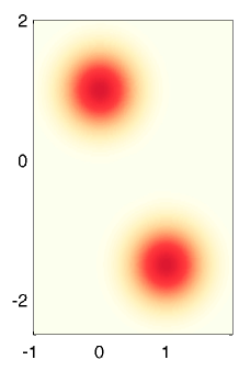
has three regions of localization as seen in the left panel of Figure 1. There are two regions around the points z1subscript𝑧1z_{1} and z2subscript𝑧2z_{2}, respectively, where the Wigner function has nonnegative Gaussian shape, whereas in between around the midpoint of z1subscript𝑧1z_{1} and z2subscript𝑧2z_{2} there is an oscillatory region with pronounced negative values.
Refer to caption
Refer to caption
Refer to caption
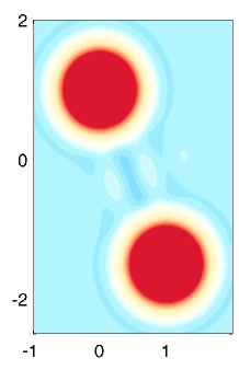
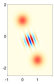
Figure 1. Contour plots of the Wigner function (left), the Husimi function (middle), and the density μψsubscript𝜇𝜓\mu_{\psi} (right) for a Gaussian superposition ψ=gz1+gz2𝜓subscript𝑔subscript𝑧1subscript𝑔subscript𝑧2\psi=g_{z_{1}}+g_{z_{2}}. We chose the phase space centers z1=(0,1)subscript𝑧101z_{1}=(0,1), z2=(1,32)subscript𝑧2132z_{2}=(1,-\tfrac{3}{2}), and the semiclassical parameter ε=0.14𝜀0.14\varepsilon=0.14. Negative values are indicated by blue color.

One way of obtaining a nonnegative phase space representation of a wave function is to convolve its Wigner function with another Wigner function. One then calls the nonnegative function

𝒲ψ𝒲ϕ,ϕ𝒮(d),subscript𝒲𝜓subscript𝒲italic-ϕitalic-ϕ𝒮superscript𝑑{\mathcal{W}}_{\psi}*{\mathcal{W}}_{\phi},\qquad\phi\in{\mathcal{S}}({\mathbb{R}}^{d}),

a spectrogram of ψ𝜓\psi. A widely used spectrogram is the Husimi function of ψ𝜓\psi,

ψ:=𝒲ψ𝒲g0,{\mathcal{H}}_{\psi}\mathrel{\mathop{:}}={\mathcal{W}}_{\psi}*{\mathcal{W}}_{g_{0}},

which is the spectrogram of ψ𝜓\psi with ϕitalic-ϕ\phi being the Gaussian wave packet g0subscript𝑔0g_{0} centered at the phase space origin. For the superposition example, the smoothing of the convolution removes the oscillations and widens the Gaussian profiles around the centers z1subscript𝑧1z_{1} and z2subscript𝑧2z_{2}; see the middle panel of Figure 1. However, the smoothing also destroys important exact relations satisfied by the Wigner function; see also [12, §7]. Let a:d:𝑎superscript𝑑a:{\mathbb{R}}^{d}\to{\mathbb{R}} be a smooth function with an appropriate decay property. Then,

da(x)|ψ(x)|2dx=2da(q)𝒲ψ(z)dz,subscriptsuperscript𝑑𝑎𝑥superscript𝜓𝑥2differential-d𝑥subscriptsuperscript2𝑑𝑎𝑞subscript𝒲𝜓𝑧differential-d𝑧\int_{{\mathbb{R}}^{d}}a(x)|\psi(x)|^{2}\,{\rm d}x=\int_{{\mathbb{R}}^{2d}}a(q){\mathcal{W}}_{\psi}(z)\,{\rm d}z,

while

da(x)|ψ(x)|2dx=2da(q)ψ(z)dz+O(ε)subscriptsuperscript𝑑𝑎𝑥superscript𝜓𝑥2differential-d𝑥subscriptsuperscript2𝑑𝑎𝑞subscript𝜓𝑧differential-d𝑧𝑂𝜀\int_{{\mathbb{R}}^{d}}a(x)|\psi(x)|^{2}\,{\rm d}x=\int_{{\mathbb{R}}^{2d}}a(q){\mathcal{H}}_{\psi}(z)\,{\rm d}z+O(\varepsilon)

as ε0𝜀0\varepsilon\to 0, where the error term depends on second and higher order derivatives of the function a𝑎a. Hence only the first moment of the position density x|ψ(x)|2maps-to𝑥superscript𝜓𝑥2x\mapsto|\psi(x)|^{2} is exactly recovered by the Husimi function.

Our aim is now to systematically construct a new phase space density that maintains some of the key properties of the Wigner function, while being amenable to sampling strategies for positive densities. We propose a proper reweighting of the Husimi function and the spectrograms obtained from the first order Hermite functions

φej(x):=(πε)d/42εxjexp(12ε|x|2),xd,j=1,,d.\varphi_{e_{j}}(x)\mathrel{\mathop{:}}=(\pi\varepsilon)^{-d/4}\sqrt{\tfrac{2}{\varepsilon}}x_{j}\exp\!\left(-\tfrac{1}{2\varepsilon}|x|^{2}\right),\qquad x\in{\mathbb{R}}^{d},\qquad j=1,\ldots,d.

We define a real-valued function μψ:2d:subscript𝜇𝜓superscript2𝑑\mu_{\psi}:{\mathbb{R}}^{2d}\to{\mathbb{R}} by

μψ:=(1+d2)𝒲ψ𝒲g012j=1d𝒲ψ𝒲φej.\mu_{\psi}\mathrel{\mathop{:}}=(1+\tfrac{d}{2}){\mathcal{W}}_{\psi}*{\mathcal{W}}_{g_{0}}-\tfrac{1}{2}\sum_{j=1}^{d}{\mathcal{W}}_{\psi}*{\mathcal{W}}_{\varphi_{e_{j}}}.

By construction, μψsubscript𝜇𝜓\mu_{\psi} is the difference of two nonnegative functions, a scalar multiple of the Husimi function 𝒲ψ𝒲g0subscript𝒲𝜓subscript𝒲subscript𝑔0{\mathcal{W}}_{\psi}*{\mathcal{W}}_{g_{0}} on the one side, and half the sum of the Hermite spectrograms 𝒲ψ𝒲φe1,,𝒲ψ𝒲φedsubscript𝒲𝜓subscript𝒲subscript𝜑subscript𝑒1subscript𝒲𝜓subscript𝒲subscript𝜑subscript𝑒𝑑{\mathcal{W}}_{\psi}*{\mathcal{W}}_{\varphi_{e_{1}}},\ldots,{\mathcal{W}}_{\psi}*{\mathcal{W}}_{\varphi_{e_{d}}} on the other side. For example, a single Gaussian wave packet ψ=gz0𝜓subscript𝑔subscript𝑧0\psi=g_{z_{0}} centered at the point z02dsubscript𝑧0superscript2𝑑z_{0}\in{\mathbb{R}}^{2d} results in

μgz0(z)subscript𝜇subscript𝑔subscript𝑧0𝑧\displaystyle\mu_{g_{z_{0}}}(z) =(1+d2)(2πε)dexp(12ε|zz0|2)absent1𝑑2superscript2𝜋𝜀𝑑12𝜀superscript𝑧subscript𝑧02\displaystyle=\left(1+\tfrac{d}{2}\right)(2\pi\varepsilon)^{-d}\exp\!\left(-\tfrac{1}{2\varepsilon}|z-z_{0}|^{2}\right)
12ε|zz0|2(2πε)dexp(12ε|zz0|2),12𝜀superscript𝑧subscript𝑧02superscript2𝜋𝜀𝑑12𝜀superscript𝑧subscript𝑧02\displaystyle\quad-\tfrac{1}{2\varepsilon}|z-z_{0}|^{2}\,(2\pi\varepsilon)^{-d}\exp\!\left(-\tfrac{1}{2\varepsilon}|z-z_{0}|^{2}\right),

which is the difference of two well-localized positive densities. For the superposition of two Gaussian wave packets ψ=gz1+gz2𝜓subscript𝑔subscript𝑧1subscript𝑔subscript𝑧2\psi=g_{z_{1}}+g_{z_{2}}, we obtain a density μψsubscript𝜇𝜓\mu_{\psi} characterized by two islands of positive values around the centers z1subscript𝑧1z_{1} and z2subscript𝑧2z_{2}, which are surrounded by a sea of negative values; see the contour plot in the right panel of Figure 1 and the explicit formula in §5.2.

The new phase space function μψsubscript𝜇𝜓\mu_{\psi} allows for the exact representation of the moments of ψ𝜓\psi up to order three in the following sense. If a:d:𝑎superscript𝑑a:{\mathbb{R}}^{d}\to{\mathbb{R}} is a polynomial of degree less than or equal to three, then

da(x)|ψ(x)|2dx=2da(q)μψ(z)dz,subscriptsuperscript𝑑𝑎𝑥superscript𝜓𝑥2differential-d𝑥subscriptsuperscript2𝑑𝑎𝑞subscript𝜇𝜓𝑧differential-d𝑧\displaystyle\int_{{\mathbb{R}}^{d}}a(x)|\psi(x)|^{2}\,{\rm d}x=\int_{{\mathbb{R}}^{2d}}a(q)\mu_{\psi}(z)\,{\rm d}z,
dψ¯(x)a(iε)ψ(x)dx=2da(p)μψ(z)dz.subscriptsuperscript𝑑¯𝜓𝑥𝑎i𝜀𝜓𝑥differential-d𝑥subscriptsuperscript2𝑑𝑎𝑝subscript𝜇𝜓𝑧differential-d𝑧\displaystyle\int_{{\mathbb{R}}^{d}}\overline{\psi}(x)a(-{\rm i}\varepsilon\nabla)\psi(x)\,{\rm d}x=\int_{{\mathbb{R}}^{2d}}a(p)\mu_{\psi}(z)\,{\rm d}z.

For arbitrary smooth functions a:2d:𝑎superscript2𝑑a:{\mathbb{R}}^{2d}\to{\mathbb{R}} and the associated Weyl quantized operator op(a)op𝑎\operatorname{op}(a), the quantum expectation value ψ,op(a)ψL2subscript𝜓op𝑎𝜓superscript𝐿2\left\langle\psi,\operatorname{op}(a)\psi\right\rangle_{L^{2}} of the observable op(a)op𝑎\operatorname{op}(a) is approximated as

(1.2) dψ¯(x)op(a)ψ(x)dx=2da(z)μψ(z)dz+O(ε2)subscriptsuperscript𝑑¯𝜓𝑥op𝑎𝜓𝑥differential-d𝑥subscriptsuperscript2𝑑𝑎𝑧subscript𝜇𝜓𝑧differential-d𝑧𝑂superscript𝜀2\int_{{\mathbb{R}}^{d}}\overline{\psi}(x)\,\operatorname{op}(a)\psi(x)\,{\rm d}x=\int_{{\mathbb{R}}^{2d}}a(z)\mu_{\psi}(z){\rm d}z+O(\varepsilon^{2})

for ε0𝜀0\varepsilon\to 0, where the error term depends on fourth and higher order derivatives of the function a𝑎a; see Theorem 3.2 later on. Phase space approximations of quantum expectations and Wigner functions play a central role in the analysis of quantum systems, in particular in the semiclassical regime; see [19, §IV] or [11, §7.1]. The idea of combining different spectrograms can also be found in the time-frequency literature; see e.g. [20] and the references given therein. However, the goal of [20] is cross-entropy optimization within a chosen set of spectrograms and not the approximation of Wigner functions or quantum expectations.

The second order accuracy with respect to ε𝜀\varepsilon in the expectation value approximation suggests using the new density in the context of molecular quantum dynamics. We consider the time-dependent Schrödinger equation

iεtψ(t)=(ε22Δ+V)ψ(t),ψ(0)=ψ0,formulae-sequencei𝜀subscript𝑡𝜓𝑡superscript𝜀22Δ𝑉𝜓𝑡𝜓0subscript𝜓0{\rm i}\varepsilon\partial_{t}\psi(t)=\left(-\tfrac{\varepsilon^{2}}{2}\Delta+V\right)\psi(t),\quad\psi(0)=\psi_{0},

with a smooth potential function V:d:𝑉superscript𝑑V:{\mathbb{R}}^{d}\to{\mathbb{R}} as provided by the time-dependent Born–Oppenheimer approximation. Let us denote by Φt:2d2d:subscriptΦ𝑡superscript2𝑑superscript2𝑑\Phi_{t}:{\mathbb{R}}^{2d}\to{\mathbb{R}}^{2d} the flow of the corresponding classical equations of motion

q˙=p,p˙=V(q).formulae-sequence˙𝑞𝑝˙𝑝𝑉𝑞\dot{q}=p,\qquad\dot{p}=-\nabla V(q).

Then, by Egorov’s theorem, we have

(1.3) ψ(t),op(a)ψ(t)L2=2d(aΦt)(z)𝒲ψ0(z)dz+O(ε2)subscript𝜓𝑡op𝑎𝜓𝑡superscript𝐿2subscriptsuperscript2𝑑𝑎subscriptΦ𝑡𝑧subscript𝒲subscript𝜓0𝑧differential-d𝑧𝑂superscript𝜀2\left\langle\psi(t),\operatorname{op}(a)\psi(t)\right\rangle_{L^{2}}=\int_{{\mathbb{R}}^{2d}}(a\circ\Phi_{t})(z){\mathcal{W}}_{\psi_{0}}(z){\rm d}z+O(\varepsilon^{2})

as ε0𝜀0\varepsilon\to 0, where the error depends on third and higher order derivatives of the functions aΦt𝑎subscriptΦ𝑡a\circ\Phi_{t} and V𝑉V as well as the L2superscript𝐿2L^{2}-norm of the initial wave function ψ0subscript𝜓0\psi_{0}. The Egorov approximation is computationally advantageous, in particular in high dimensions, since it allows to simulate the time-evolution of quantum expectations by an ensemble of classical trajectories. Over decades, it has been widely used in the physical chemistry literature under the name linearized semiclassical initial value representation (LSC-IVR) or Wigner phase space method.

Our new phase space density comes into play here, since the combination of the approximations in (1.2) and (1.3) provides

ψ(t),op(a)ψ(t)L2=2d(aΦt)(z)μψ0(z)dz+O(ε2),subscript𝜓𝑡op𝑎𝜓𝑡superscript𝐿2subscriptsuperscript2𝑑𝑎subscriptΦ𝑡𝑧subscript𝜇subscript𝜓0𝑧differential-d𝑧𝑂superscript𝜀2\left\langle\psi(t),\operatorname{op}(a)\psi(t)\right\rangle_{L^{2}}=\int_{{\mathbb{R}}^{2d}}(a\circ\Phi_{t})(z)\mu_{\psi_{0}}(z){\rm d}z+O(\varepsilon^{2}),

which can be read as a new method for the computation of time-evolved quantum expectations by initial sampling from a difference of nonnegative phase space distributions; see Theorem 4.1 and the numerical experiments in §6.

1.1. Outline

Our investigation proceeds along the following lines. In §2 we briefly review phase space distributions as the Wigner function, spectrograms, and the Husimi function. §3 derives the new phase space density μψsubscript𝜇𝜓\mu_{\psi} and proves our main result, that is, the second order approximation of expectation values by the phase space integration with respect to the new density function. §4 applies this result to the quantum propagation of expectation values. Then, several explicit formulas for the density μψsubscript𝜇𝜓\mu_{\psi} are derived in §5. The numerical experiments in §6 illustrate the applicability of the new approach for the dynamics of molecular quantum systems in dimensions d=1𝑑1d=1, d=2𝑑2d=2, and d=32𝑑32d=32. Appendix A presents a sampling strategy for the density μψsubscript𝜇𝜓\mu_{\psi} via the Gamma distribution used for the numerical experiments, while Appendix B provides further computational details.

2. Phase space distributions

In this section we review different possibilities for representing a square integrable function ψL2(d)𝜓superscript𝐿2superscript𝑑\psi\in L^{2}({{\mathbb{R}}^{d}}) via real-valued distributions on the classical phase space Td2dsuperscript𝑇superscript𝑑superscript2𝑑T^{*}{\mathbb{R}}^{d}\cong{{\mathbb{R}}^{2d}}. Considering functions with frequencies of the order 1/ε1𝜀1/\varepsilon for a small parameter 0<ε10𝜀much-less-than10<\varepsilon\ll 1, we work with the ε𝜀\varepsilon-rescaled Fourier transform

εψ(p):=(2πε)d/2dψ(q)eipq/εdq,pd.\mathcal{F}_{\varepsilon}\psi(p)\mathrel{\mathop{:}}=(2\pi\varepsilon)^{-d/2}\int_{{\mathbb{R}}^{d}}\psi(q){\rm e}^{-{\rm i}p\cdot q/\varepsilon}{\rm d}q,\qquad p\in{\mathbb{R}}^{d}.

We also use the Heisenberg–Weyl operator in ε𝜀\varepsilon-scaling:

Definition 2.1.

The Heisenberg–Weyl operator associated with a phase space point z=(q,p)2d𝑧𝑞𝑝superscript2𝑑z=(q,p)\in{{\mathbb{R}}^{2d}} is defined as

Tzψ:=eip(q/2)/εψ(q),ψL2(d).T_{z}\psi\mathrel{\mathop{:}}={\rm e}^{{\rm i}p\cdot(\bullet-q/2)/\varepsilon}\psi(\bullet-q),\qquad\psi\in L^{2}({\mathbb{R}}^{d}).

Among its many striking properties, the following two will be important for us later on. We have

Tz=Tz,z2d,formulae-sequencesuperscriptsubscript𝑇𝑧subscript𝑇𝑧𝑧superscript2𝑑T_{z}^{\dagger}=T_{-z},\qquad z\in{{\mathbb{R}}^{2d}},

and

Tz1Tz2=exp(i2εΩ(z1,z2))Tz1+z2,z1,z22d,formulae-sequencesubscript𝑇subscript𝑧1subscript𝑇subscript𝑧2i2𝜀Ωsubscript𝑧1subscript𝑧2subscript𝑇subscript𝑧1subscript𝑧2subscript𝑧1subscript𝑧2superscript2𝑑T_{z_{1}}T_{z_{2}}=\exp{\left(-\tfrac{{\rm i}}{2\varepsilon}\Omega(z_{1},z_{2})\right)}\,T_{z_{1}+z_{2}},\qquad z_{1},z_{2}\in{{\mathbb{R}}^{2d}},

where Ω:2d×2d:Ωsuperscript2𝑑superscript2𝑑\Omega:{{\mathbb{R}}^{2d}}\times{{\mathbb{R}}^{2d}}\to{\mathbb{R}} denotes the standard symplectic form on 2dsuperscript2𝑑{{\mathbb{R}}^{2d}}, i.e.,

(2.1) Ω(z1,z2):=z1TJz2=q1Tp2p1Tq2withJ=[0IdId0].\Omega(z_{1},z_{2})\mathrel{\mathop{:}}=z_{1}^{T}Jz_{2}=q_{1}^{T}p_{2}-p_{1}^{T}q_{2}\qquad\text{with}\qquad J=\begin{bmatrix}0&{\rm Id}\\ -{\rm Id}&0\end{bmatrix}.

All phase space distributions considered here turn the action of the Heisenberg–Weyl operator Tzsubscript𝑇𝑧T_{z} on a wave function into a phase space translation by z𝑧z, which is often referred to as a covariance property; see, e.g., (2.6) below.

Remark 2.2.

The Gaussian wave packet (1.1) with its phase space center at z02dsubscript𝑧0superscript2𝑑z_{0}\in{\mathbb{R}}^{2d} is obtained by applying the Heisenberg–Weyl operator Tz0subscript𝑇subscript𝑧0T_{z_{0}} to the Gaussian

g0(x):=(πε)d/4exp(12ε|x|2)g_{0}(x)\mathrel{\mathop{:}}=(\pi\varepsilon)^{-d/4}\exp\!\left(-\tfrac{1}{2\varepsilon}|x|^{2}\right)

centered at the origin, i.e., gz0=Tz0g0subscript𝑔subscript𝑧0subscript𝑇subscript𝑧0subscript𝑔0g_{z_{0}}=T_{z_{0}}g_{0}.

2.1. Wigner functions

We start our discussion with the celebrated Wigner function and recapitulate some basic relations.

Definition 2.3.

The Wigner function of a function ψL2(d)𝜓superscript𝐿2superscript𝑑\psi\in L^{2}({\mathbb{R}}^{d}) is defined as 𝒲ψ:2d:subscript𝒲𝜓superscript2𝑑{\mathcal{W}}_{\psi}:{{\mathbb{R}}^{2d}}\to{\mathbb{R}},

𝒲ψ(z):=(2πε)ddψ¯(q+y2)ψ(qy2)eiyp/εdy,z=(q,p)2d.{\mathcal{W}}_{\psi}(z)\mathrel{\mathop{:}}=(2\pi\varepsilon)^{-d}\int_{{\mathbb{R}}^{d}}\overline{\psi}(q+\tfrac{y}{2})\psi(q-\tfrac{y}{2}){\rm e}^{{\rm i}y\cdot p/\varepsilon}{\rm d}y,\qquad z=(q,p)\in{\mathbb{R}}^{2d}.

Wigner functions are continuous square-integrable functions on phase space; however, they need not be integrable. The marginals are the position and momentum density of the state, respectively. With a proper interpretation of the possibly not absolutely convergent integrals this means

d𝒲ψ(q,p)dp=|ψ(q)|2,d𝒲ψ(q,p)dq=|εψ(p)|2,formulae-sequencesubscriptsuperscript𝑑subscript𝒲𝜓𝑞𝑝differential-d𝑝superscript𝜓𝑞2subscriptsuperscript𝑑subscript𝒲𝜓𝑞𝑝differential-d𝑞superscriptsubscript𝜀𝜓𝑝2\int_{{\mathbb{R}}^{d}}{\mathcal{W}}_{\psi}(q,p){\rm d}p=|\psi(q)|^{2},\qquad\int_{{\mathbb{R}}^{d}}{\mathcal{W}}_{\psi}(q,p){\rm d}q=|\mathcal{F}_{\varepsilon}\psi(p)|^{2},

and in particular

2d𝒲ψ(z)dz=ψ2.subscriptsuperscript2𝑑subscript𝒲𝜓𝑧differential-d𝑧superscriptnorm𝜓2\int_{{\mathbb{R}}^{2d}}{\mathcal{W}}_{\psi}(z){\rm d}z=\|\psi\|^{2}.

Wigner transformation preserves orthogonality in the sense that

2d𝒲ψ(z)𝒲ϕ(z)dz=(2πε)d|ψ,ϕ|,ψ,ϕL2(d),formulae-sequencesubscriptsuperscript2𝑑subscript𝒲𝜓𝑧subscript𝒲italic-ϕ𝑧differential-d𝑧superscript2𝜋𝜀𝑑𝜓italic-ϕ𝜓italic-ϕsuperscript𝐿2superscript𝑑\int_{{{\mathbb{R}}^{2d}}}{\mathcal{W}}_{\psi}(z){\mathcal{W}}_{\phi}(z){\rm d}z=(2\pi\varepsilon)^{-d}\left|\langle\psi,\phi\rangle\right|,\qquad\psi,\phi\in L^{2}({\mathbb{R}}^{d}),

and it turns the action of the Heisenberg–Weyl operator into a phase space translation, i.e.,

𝒲Tzψ=𝒲ψ(z),z2d,{\mathcal{W}}_{T_{z}\psi}={\mathcal{W}}_{\psi}(\bullet-z),\qquad z\in{\mathbb{R}}^{2d},

which is an example of the covariance property alluded above.

Moreover, given a Schwartz function a:2d:𝑎superscript2𝑑a:{{\mathbb{R}}^{2d}}\to{\mathbb{R}}, one can use Wigner functions to express expectation values of Weyl quantized linear operators

(2.2) (op(a)ψ)(q)=(2πε)d2da(q+y2,p)ψ(y)ei(qy)p/εdydpop𝑎𝜓𝑞superscript2𝜋𝜀𝑑subscriptsuperscript2𝑑𝑎𝑞𝑦2𝑝𝜓𝑦superscriptei𝑞𝑦𝑝𝜀differential-d𝑦differential-d𝑝(\operatorname{op}(a)\psi)(q)=(2\pi\varepsilon)^{-d}\int_{{\mathbb{R}}^{2d}}a(\tfrac{q+y}{2},p)\psi(y){\rm e}^{{\rm i}(q-y)\cdot p/\varepsilon}{\rm d}y\,{\rm d}p

via the weighted phase space integral

(2.3) ψ,op(a)ψ=2da(z)𝒲ψ(z)dz.𝜓op𝑎𝜓subscriptsuperscript2𝑑𝑎𝑧subscript𝒲𝜓𝑧differential-d𝑧\left\langle\psi,\operatorname{op}(a)\psi\right\rangle=\int_{{\mathbb{R}}^{2d}}a(z){\mathcal{W}}_{\psi}(z){\rm d}z.

We note that the oscillatory integral formula (2.2) can be extended to more general classes of symbols a:2d:𝑎superscript2𝑑a:{{\mathbb{R}}^{2d}}\to{\mathbb{R}} with controlled growth properties at infinity; see for example [28, §4], [21, §2] or [9, §2].

2.2. Spectrograms

Except for Gaussian states, Wigner functions attain negative values (see [26]), and thus cannot be treated as probability densities. For example, any odd function ψL2(d)𝜓superscript𝐿2superscript𝑑\psi\in L^{2}({\mathbb{R}}^{d}) satisfies

𝒲ψ(0)=(2πε)dd|ψ(y2)|2dy0.subscript𝒲𝜓0superscript2𝜋𝜀𝑑subscriptsuperscript𝑑superscript𝜓𝑦22differential-d𝑦0{\mathcal{W}}_{\psi}(0)=-(2\pi\varepsilon)^{-d}\int_{{\mathbb{R}}^{d}}|\psi(\tfrac{y}{2})|^{2}\,{\rm d}y\leq 0.

One way to obtain nonnegative phase space representations of a quantum state is to convolve its Wigner function with another Wigner function.

Definition 2.4.

Let ψL2(d)𝜓superscript𝐿2superscript𝑑\psi\in L^{2}({{\mathbb{R}}^{d}}) and ϕ𝒮(d)italic-ϕ𝒮superscript𝑑\phi\in{\mathcal{S}}({{\mathbb{R}}^{d}}). Then, 𝒲ψ𝒲ϕsubscript𝒲𝜓subscript𝒲italic-ϕ{\mathcal{W}}_{\psi}*{\mathcal{W}}_{\phi} is called a spectrogram of ψ𝜓\psi.

In time-frequency analysis, spectrograms are typically introduced as the modulus squared of a short-time Fourier transform (see, e.g., the introduction in [8]) so that the representation via the convolution of two Wigner transforms is derived subsequently. Spectrograms also form a sub-class of Cohen’s class of phase space distributions [6, §3.2.1.]. They satisfy

(2.4) (𝒲ψ𝒲ϕ)(z)=(2πε)d|Tzϕ,ψ|2,z2d,formulae-sequencesubscript𝒲𝜓subscript𝒲italic-ϕ𝑧superscript2𝜋𝜀𝑑superscriptsubscript𝑇𝑧subscriptitalic-ϕ𝜓2𝑧superscript2𝑑({\mathcal{W}}_{\psi}*{\mathcal{W}}_{\phi})(z)=(2\pi\varepsilon)^{-d}\left|\langle T_{z}\phi_{-},\psi\rangle\right|^{2},\qquad z\in{\mathbb{R}}^{2d},

where ϕ(x):=ϕ(x)\phi_{-}(x)\mathrel{\mathop{:}}=\phi(-x) for xd𝑥superscript𝑑x\in{\mathbb{R}}^{d}; see also [9, Proposition 1.99]. Thus, spectrograms are nonnegative and smooth by construction. The integrability follows from (2.4) by the square integrability of general Fourier-Wigner transforms zTzϕ,ψmaps-to𝑧subscript𝑇𝑧italic-ϕ𝜓z\mapsto\langle T_{z}\phi,\psi\rangle with ϕ,ψL2(d)italic-ϕ𝜓superscript𝐿2superscript𝑑\phi,\psi\in L^{2}({{\mathbb{R}}^{d}}), see Proposition 1.42 in [9]. Normalization is preserved according to

(2.5) 2d(𝒲ψ𝒲ϕ)(z)dz=ψ2ϕ2.subscriptsuperscript2𝑑subscript𝒲𝜓subscript𝒲italic-ϕ𝑧differential-d𝑧superscriptnorm𝜓2superscriptnormitalic-ϕ2\int_{{\mathbb{R}}^{2d}}({\mathcal{W}}_{\psi}*{\mathcal{W}}_{\phi})(z){\rm d}z=\|\psi\|^{2}\cdot\|\phi\|^{2}.

Spectrograms also inherit the covariance property from the Wigner function, i.e.,

(2.6) 𝒲Tzψ𝒲ϕ=(𝒲ψ𝒲ϕ)(z),z2d.{\mathcal{W}}_{T_{z}\psi}*{\mathcal{W}}_{\phi}=({\mathcal{W}}_{\psi}*{\mathcal{W}}_{\phi})(\bullet-z),\qquad z\in{\mathbb{R}}^{2d}.

A particular spectrogram is obtained by convolving with the Wigner function of a Gaussian wave packet, which we will discuss next.

2.3. Husimi functions

The most commonly used nonnegative phase space distribution is the Husimi function; see e.g. [2, §4.1]. We consider the Wigner function

𝒲g0(z)=(πε)de|z|2/ε,z2d,formulae-sequencesubscript𝒲subscript𝑔0𝑧superscript𝜋𝜀𝑑superscriptesuperscript𝑧2𝜀𝑧superscript2𝑑{\mathcal{W}}_{g_{0}}(z)=(\pi\varepsilon)^{-d}{\rm e}^{-|z|^{2}/\varepsilon},\qquad z\in{{\mathbb{R}}^{2d}},

of the Gaussian wave packet g0subscript𝑔0g_{0} centered at the phase space origin and define:

Definition 2.5.

The Husimi function of ψL2(d)𝜓superscript𝐿2superscript𝑑\psi\in L^{2}({\mathbb{R}}^{d}) is defined as the spectrogram

ψ(z):=(𝒲ψ𝒲g0)(z)=2d𝒲ψ(w)(πε)de|zw|2/εdw.{\mathcal{H}}_{\psi}(z)\mathrel{\mathop{:}}=({\mathcal{W}}_{\psi}*{\mathcal{W}}_{g_{0}})(z)=\int_{{{\mathbb{R}}^{2d}}}{\mathcal{W}}_{\psi}(w)\,(\pi\varepsilon)^{-d}{\rm e}^{-|z-w|^{2}/\varepsilon}\,{\rm d}{w}.

The Husimi function of ψ𝜓\psi is the spectrogram (2.4) with ϕitalic-ϕ\phi being the Gaussian wave packet g0subscript𝑔0g_{0}, and since g0subscript𝑔0g_{0} is even, we have

ψ(z)=(2πε)d|Tzg0,ψ|2,z2d.formulae-sequencesubscript𝜓𝑧superscript2𝜋𝜀𝑑superscriptsubscript𝑇𝑧subscript𝑔0𝜓2𝑧superscript2𝑑{\mathcal{H}}_{\psi}(z)=(2\pi\varepsilon)^{-d}\left|\langle T_{z}g_{0},\psi\rangle\right|^{2},\qquad z\in{{\mathbb{R}}^{2d}}.

Also, since g0subscript𝑔0g_{0} is normalized, i.e., g0=1normsubscript𝑔01\|g_{0}\|=1, (2.5) gives

2dψ(z)dz=ψ2.subscriptsuperscript2𝑑subscript𝜓𝑧differential-d𝑧superscriptnorm𝜓2\int_{{\mathbb{R}}^{2d}}{\mathcal{H}}_{\psi}(z){\rm d}z=\|\psi\|^{2}.

That is, for ψL2(d)𝜓superscript𝐿2superscript𝑑\psi\in L^{2}({{\mathbb{R}}^{d}}) with ψ=1norm𝜓1\|\psi\|=1, the Husimi function is a smooth probability density on phase space.

Remark 2.6.

The Husimi function of ψL2(d)𝜓superscript𝐿2superscript𝑑\psi\in L^{2}({\mathbb{R}}^{d}) is the modulus squared of the so-called Fourier–Bros–Iagolnitzer (FBI) transform, which associates with ψ𝜓\psi the mapping

2d,z(2πε)d/2Tzg0,ψ.formulae-sequencesuperscript2𝑑maps-to𝑧superscript2𝜋𝜀𝑑2subscript𝑇𝑧subscript𝑔0𝜓{{\mathbb{R}}^{2d}}\to{\mathbb{C}},\quad z\mapsto(2\pi\varepsilon)^{-d/2}\langle T_{z}g_{0},\psi\rangle.

In contrast to the Wigner function and the spectrograms, the FBI transform is a linear, albeit complex-valued phase space representation; see [21, Chapter 3].

Integrating a Schwartz function a:2d:𝑎superscript2𝑑a:{{\mathbb{R}}^{2d}}\to{\mathbb{R}} against the Husimi function, we obtain

2da(z)ψ(z)dzsubscriptsuperscript2𝑑𝑎𝑧subscript𝜓𝑧differential-d𝑧\displaystyle\int_{{\mathbb{R}}^{2d}}a(z){\mathcal{H}}_{\psi}(z){\rm d}z =2da(z)(𝒲ψ𝒲g0)(z)dz=2d(a𝒲g0)(z)𝒲ψ(z)dzabsentsubscriptsuperscript2𝑑𝑎𝑧subscript𝒲𝜓subscript𝒲subscript𝑔0𝑧differential-d𝑧subscriptsuperscript2𝑑𝑎subscript𝒲subscript𝑔0𝑧subscript𝒲𝜓𝑧differential-d𝑧\displaystyle=\int_{{\mathbb{R}}^{2d}}a(z)({\mathcal{W}}_{\psi}*{\mathcal{W}}_{g_{0}})(z){\rm d}z=\int_{{\mathbb{R}}^{2d}}(a*{\mathcal{W}}_{g_{0}})(z){\mathcal{W}}_{\psi}(z){\rm d}z
=ψ,op(a𝒲g0)ψ,absent𝜓op𝑎subscript𝒲subscript𝑔0𝜓\displaystyle=\left\langle\psi,\operatorname{op}(a*{\mathcal{W}}_{g_{0}})\psi\right\rangle,

where the last equation uses the duality relation (2.3) between Weyl quantized operators and the Wigner transform. Therefore,

2da(z)ψ(z)dz=ψ,opaw(a)ψ,subscriptsuperscript2𝑑𝑎𝑧subscript𝜓𝑧differential-d𝑧𝜓subscriptopaw𝑎𝜓\int_{{\mathbb{R}}^{2d}}a(z){\mathcal{H}}_{\psi}(z){\rm d}z=\langle\psi,\operatorname{op}_{\rm aw}(a)\psi\rangle,

where

opaw(a):=op(a𝒲g0),a𝒮(2d),\operatorname{op}_{\rm aw}(a)\mathrel{\mathop{:}}=\operatorname{op}(a*{\mathcal{W}}_{g_{0}}),\qquad a\in{\mathcal{S}}({{\mathbb{R}}^{2d}}),

denotes the anti-Wick quantized operator of the function a𝑎a; see for example [9, §2.7] and [4, §11.4]. Weyl and anti-Wick quantization are ε𝜀\varepsilon-close in the following sense:

Lemma 2.7.

Let a:2d:𝑎superscript2𝑑a:{{\mathbb{R}}^{2d}}\to{\mathbb{R}} be a Schwartz function and ε>0𝜀0\varepsilon>0. Then, there are two families of Schwartz functions r1ε,r2ε:2d:subscriptsuperscript𝑟𝜀1subscriptsuperscript𝑟𝜀2superscript2𝑑r^{\varepsilon}_{1},r^{\varepsilon}_{2}:{{\mathbb{R}}^{2d}}\to{\mathbb{R}} that depend on fourth and higher order derivatives of a𝑎a, so that

opaw(a)subscriptopaw𝑎\displaystyle\operatorname{op}_{\rm aw}(a) =op(a+ε4Δa)+ε2op(r1ε),absentop𝑎𝜀4Δ𝑎superscript𝜀2opsubscriptsuperscript𝑟𝜀1\displaystyle=\operatorname{op}(a+\tfrac{\varepsilon}{4}\Delta a)+\varepsilon^{2}\operatorname{op}(r^{\varepsilon}_{1}),
opaw(aε4Δa)subscriptopaw𝑎𝜀4Δ𝑎\displaystyle\operatorname{op}_{\rm aw}(a-\tfrac{\varepsilon}{4}\Delta a) =op(a)+ε2op(r2ε),absentop𝑎superscript𝜀2opsubscriptsuperscript𝑟𝜀2\displaystyle=\operatorname{op}(a)+\varepsilon^{2}\operatorname{op}(r^{\varepsilon}_{2}),

where supε>0op(rjε)L2L2<subscriptsupremum𝜀0subscriptnormopsubscriptsuperscript𝑟𝜀𝑗superscript𝐿2superscript𝐿2\sup_{\varepsilon>0}\|\operatorname{op}(r^{\varepsilon}_{j})\|_{L^{2}\to L^{2}}<\infty for both j=1,2𝑗12j=1,2.

Proof.

The lemma is essentially proven in [18, Proposition 2.4.3] or [14, Lemma 1], and hence we only sketch the proof for the second of the two equivalent identities. We write out the definition

opaw(aε4Δa)subscriptopaw𝑎𝜀4Δ𝑎\displaystyle\operatorname{op}_{\rm aw}(a-\tfrac{\varepsilon}{4}\Delta a) =op(𝒲g0(aε4Δa))absentopsubscript𝒲subscript𝑔0𝑎𝜀4Δ𝑎\displaystyle=\operatorname{op}\left({\mathcal{W}}_{g_{0}}*(a-\tfrac{\varepsilon}{4}\Delta a)\right)

and Taylor expand aε4Δa𝑎𝜀4Δ𝑎a-\tfrac{\varepsilon}{4}\Delta a around z𝑧z in the integral

𝒲g0(aε4Δa)=(πε)d2d(aε4Δa)(ζ)e|zζ|2/εdζ.subscript𝒲subscript𝑔0𝑎𝜀4Δ𝑎superscript𝜋𝜀𝑑subscriptsuperscript2𝑑𝑎𝜀4Δ𝑎𝜁superscriptesuperscript𝑧𝜁2𝜀differential-d𝜁{\mathcal{W}}_{g_{0}}*(a-\tfrac{\varepsilon}{4}\Delta a)=(\pi\varepsilon)^{-d}\int_{{\mathbb{R}}^{2d}}(a-\tfrac{\varepsilon}{4}\Delta a)(\zeta){\rm e}^{-|z-\zeta|^{2}/\varepsilon}{\rm d}\zeta.

Due to the symmetry of the Gaussian, all Taylor expansion terms with odd derivatives of (aε4Δa)𝑎𝜀4Δ𝑎(a-\tfrac{\varepsilon}{4}\Delta a) vanish. The computation

(πε)d|α|=12d1(2α)!(2α(aε4Δa))(ζz)2αe|zζ|2/εdζ=ε4Δ(aε4Δa)superscript𝜋𝜀𝑑subscript𝛼1subscriptsuperscript2𝑑12𝛼superscript2𝛼𝑎𝜀4Δ𝑎superscript𝜁𝑧2𝛼superscriptesuperscript𝑧𝜁2𝜀differential-d𝜁𝜀4Δ𝑎𝜀4Δ𝑎(\pi\varepsilon)^{-d}\sum_{|\alpha|=1}\int_{{\mathbb{R}}^{2d}}\frac{1}{(2\alpha)!}(\partial^{2\alpha}(a-\tfrac{\varepsilon}{4}\Delta a))(\zeta-z)^{2\alpha}{\rm e}^{-|z-\zeta|^{2}/\varepsilon}{\rm d}\zeta=\frac{\varepsilon}{4}\Delta(a-\tfrac{\varepsilon}{4}\Delta a)

implies the second order approximation

𝒲g0(aε4Δa)subscript𝒲subscript𝑔0𝑎𝜀4Δ𝑎\displaystyle{\mathcal{W}}_{g_{0}}*(a-\tfrac{\varepsilon}{4}\Delta a) =(aε4Δa)+ε4Δ(aε4Δa)+O(ε2)absent𝑎𝜀4Δ𝑎𝜀4Δ𝑎𝜀4Δ𝑎𝑂superscript𝜀2\displaystyle=(a-\tfrac{\varepsilon}{4}\Delta a)+\tfrac{\varepsilon}{4}\Delta(a-\tfrac{\varepsilon}{4}\Delta a)+O(\varepsilon^{2})
=a+O(ε2),absent𝑎𝑂superscript𝜀2\displaystyle=a+O(\varepsilon^{2}),

where the O(ε2)𝑂superscript𝜀2O(\varepsilon^{2}) term is of Schwartz class. Applying the Calderón–Vaillancourt Theorem (see, e.g., [9, §2.5]) concludes the proof. ∎

Remark 2.8.

The result of Lemma 2.7 can formally be read in terms of the heat semigroup {exp(tΔ)}t0subscript𝑡Δ𝑡0\{\exp(t\Delta)\}_{t\geq 0} as

a𝒲g0=exp(ε4Δ)a=a+ε4Δa+O(ε2),𝑎subscript𝒲subscript𝑔0𝜀4Δ𝑎𝑎𝜀4Δ𝑎𝑂superscript𝜀2a*{\mathcal{W}}_{g_{0}}=\exp(\tfrac{\varepsilon}{4}\Delta)a=a+\tfrac{\varepsilon}{4}\Delta a+O(\varepsilon^{2}),

where a:2d:𝑎superscript2𝑑a:{{\mathbb{R}}^{2d}}\to{\mathbb{R}} is a Schwartz function.

3. The new phase space density

We learn from the preceding discussion of phase space distributions, in particular from Lemma 2.7, that the Husimi function allows to approximate an expectation value according to

ψ,op(a)ψ=2d(aε4Δa)(z)ψ(z)dz+O(ε2)𝜓op𝑎𝜓subscriptsuperscript2𝑑𝑎𝜀4Δ𝑎𝑧subscript𝜓𝑧differential-d𝑧𝑂superscript𝜀2\left\langle\psi,\operatorname{op}(a)\psi\right\rangle=\int_{{\mathbb{R}}^{2d}}(a-\tfrac{\varepsilon}{4}\Delta a)(z){\mathcal{H}}_{\psi}(z){\rm d}z+O(\varepsilon^{2})

as ε0𝜀0\varepsilon\to 0, where the error depends on the fourth and higher order derivatives of a𝑎a and the L2superscript𝐿2L^{2}-norm of ψ𝜓\psi. An integration by parts provides

ψ,op(a)ψ=2da(z)(ψε4Δψ)(z)dz+O(ε2),𝜓op𝑎𝜓subscriptsuperscript2𝑑𝑎𝑧subscript𝜓𝜀4Δsubscript𝜓𝑧differential-d𝑧𝑂superscript𝜀2\left\langle\psi,\operatorname{op}(a)\psi\right\rangle=\int_{{\mathbb{R}}^{2d}}a(z)\,({\mathcal{H}}_{\psi}-\tfrac{\varepsilon}{4}\Delta{\mathcal{H}}_{\psi})(z)\,{\rm d}z+O(\varepsilon^{2}),

and motivates us to define the following new phase space density.

Definition 3.1.

For ψL2(d)𝜓superscript𝐿2superscript𝑑\psi\in L^{2}({{\mathbb{R}}^{d}}) we define the phase space density μψ:2d:subscript𝜇𝜓superscript2𝑑\mu_{\psi}:{{\mathbb{R}}^{2d}}\to{\mathbb{R}},

μψsubscript𝜇𝜓\displaystyle\mu_{\psi} :=ψε4Δψ.\displaystyle\mathrel{\mathop{:}}={\mathcal{H}}_{\psi}-\tfrac{\varepsilon}{4}\Delta{\mathcal{H}}_{\psi}.

We summarize the key property of the new density as follows:

Theorem 3.2.

Let a:2d:𝑎superscript2𝑑a:{{\mathbb{R}}^{2d}}\to{\mathbb{R}} be a Schwartz function. Then, there exists a constant C0𝐶0C\geq 0 depending on fourth and higher order derivatives of a𝑎a such that for all ψL2(d)𝜓superscript𝐿2superscript𝑑\psi\in L^{2}({{\mathbb{R}}^{d}})

|ψ,op(a)ψ2da(z)μψ(z)dz|Cε2ψ2,𝜓op𝑎𝜓subscriptsuperscript2𝑑𝑎𝑧subscript𝜇𝜓𝑧differential-d𝑧𝐶superscript𝜀2superscriptnorm𝜓2\left|\langle\psi,\operatorname{op}(a)\psi\rangle-\int_{{\mathbb{R}}^{2d}}a(z)\mu_{\psi}(z){\rm d}z\right|\leq C\varepsilon^{2}\|\psi\|^{2},

where the density μψ:2d:subscript𝜇𝜓superscript2𝑑\mu_{\psi}:{{\mathbb{R}}^{2d}}\to{\mathbb{R}} was defined in Definition 3.1.

Proof.

By Lemma 2.7, we have

ψ,op(a)ψ=2d(aε4Δa)(z)ψ(z)dz+ε2ψ,op(rε)ψ𝜓op𝑎𝜓subscriptsuperscript2𝑑𝑎𝜀4Δ𝑎𝑧subscript𝜓𝑧differential-d𝑧superscript𝜀2𝜓opsuperscript𝑟𝜀𝜓\langle\psi,\operatorname{op}(a)\psi\rangle=\int_{{\mathbb{R}}^{2d}}(a-\tfrac{\varepsilon}{4}\Delta a)(z){\mathcal{H}}_{\psi}(z){\rm d}z+\varepsilon^{2}\langle\psi,\operatorname{op}(r^{\varepsilon})\psi\rangle

with

|ψ,op(rε)ψ|Cψ2,𝜓opsuperscript𝑟𝜀𝜓𝐶superscriptnorm𝜓2|\langle\psi,\operatorname{op}(r^{\varepsilon})\psi\rangle|\;\leq\;C\|\psi\|^{2},

where the constant C>0𝐶0C>0 depends on the fourth and higher order derivatives of a𝑎a. The Husimi function ψsubscript𝜓{\mathcal{H}}_{\psi} is smooth and bounded since

ψ(z)=(2πε)d|gz,ψ|2(2πε)dgz2ψ2=(2πε)dψ2.subscript𝜓𝑧superscript2𝜋𝜀𝑑superscriptsubscript𝑔𝑧𝜓2superscript2𝜋𝜀𝑑superscriptnormsubscript𝑔𝑧2superscriptnorm𝜓2superscript2𝜋𝜀𝑑superscriptnorm𝜓2{\mathcal{H}}_{\psi}(z)=(2\pi\varepsilon)^{-d}\left|\langle g_{z},\psi\rangle\right|^{2}\leq(2\pi\varepsilon)^{-d}{\left\|g_{z}\right\|}^{2}{\left\|\psi\right\|}^{2}=(2\pi\varepsilon)^{-d}{\left\|\psi\right\|}^{2}.

Hence, integration by parts implies

2d(aε4Δa)(z)ψ(z)dz=2da(z)(ψε4Δψ)(z)dz=2da(z)μψ(z)dz.subscriptsuperscript2𝑑𝑎𝜀4Δ𝑎𝑧subscript𝜓𝑧differential-d𝑧subscriptsuperscript2𝑑𝑎𝑧subscript𝜓𝜀4Δsubscript𝜓𝑧differential-d𝑧subscriptsuperscript2𝑑𝑎𝑧subscript𝜇𝜓𝑧differential-d𝑧\int_{{\mathbb{R}}^{2d}}(a-\tfrac{\varepsilon}{4}\Delta a)(z){\mathcal{H}}_{\psi}(z){\rm d}z=\int_{{\mathbb{R}}^{2d}}a(z)({\mathcal{H}}_{\psi}-\tfrac{\varepsilon}{4}\Delta{\mathcal{H}}_{\psi})(z){\rm d}z=\int_{{\mathbb{R}}^{2d}}a(z)\mu_{\psi}(z){\rm d}z.

Therefore,

|ψ,op(a)ψ2da(z)μψ(z)dz|=ε2|ψ,op(rε)ψ|Cε2ψ2,𝜓op𝑎𝜓subscriptsuperscript2𝑑𝑎𝑧subscript𝜇𝜓𝑧differential-d𝑧superscript𝜀2𝜓opsuperscript𝑟𝜀𝜓𝐶superscript𝜀2superscriptnorm𝜓2\left|\langle\psi,\operatorname{op}(a)\psi\rangle-\int_{{\mathbb{R}}^{2d}}a(z)\mu_{\psi}(z){\rm d}z\right|=\varepsilon^{2}|\langle\psi,\operatorname{op}(r^{\varepsilon})\psi\rangle|\;\leq\;C\,\varepsilon^{2}\|\psi\|^{2},

which concludes the proof. ∎

Remark 3.3.

Whenever a:2d:𝑎superscript2𝑑a:{{\mathbb{R}}^{2d}}\to{\mathbb{R}} is a polynomial of degree less than or equal to three, the constant C0𝐶0C\geq 0 of Theorem 3.2 vanishes so that the phase space integration with respect to μψsubscript𝜇𝜓\mu_{\psi} exactly reproduces the expectation value. Moreover, using higher order Hermite spectrograms, one can also construct densities which yield approximations of expectation values with higher order errors in ε𝜀\varepsilon, or, equivalently, which are exact for polynomial symbols a:2d:𝑎superscript2𝑑a:{{\mathbb{R}}^{2d}}\to{\mathbb{R}} of higher degree. We refer to the thesis [13, §10.5] for the next order result and an outline on how to prove higher order approximations.

Our next aim is to derive an alternative expression for the new density showing that it is a linear combination of spectrograms.

3.1. The new density in terms of Hermite functions

The Laplacian of the Husimi function can be related to the Wigner function of the ε𝜀\varepsilon-rescaled first order Hermite functions as follows:

Proposition 3.4.

Let ε>0𝜀0\varepsilon>0, j{1,,d}𝑗1𝑑j\in\{1,\ldots,d\}, and

φej(x):=(πε)d/42εxjexp(12ε|x|2),xd,\varphi_{e_{j}}(x)\mathrel{\mathop{:}}=(\pi\varepsilon)^{-d/4}\sqrt{\tfrac{2}{\varepsilon}}x_{j}\exp\!\left(-\tfrac{1}{2\varepsilon}|x|^{2}\right),\qquad x\in{\mathbb{R}}^{d},

be the first order Hermite functions. Then, for all ψL2(d)𝜓superscript𝐿2superscript𝑑\psi\in L^{2}({{\mathbb{R}}^{d}}),

Δψ=2εj=1d𝒲ψ𝒲φej2dεψΔsubscript𝜓2𝜀superscriptsubscript𝑗1𝑑subscript𝒲𝜓subscript𝒲subscript𝜑subscript𝑒𝑗2𝑑𝜀subscript𝜓\Delta{\mathcal{H}}_{\psi}=\tfrac{2}{\varepsilon}\sum_{j=1}^{d}{\mathcal{W}}_{\psi}*{\mathcal{W}}_{\varphi_{e_{j}}}-\tfrac{2d}{\varepsilon}{\mathcal{H}}_{\psi}

and consequently

μψ=ψε4Δψ=(1+d2)ψ12j=1d𝒲ψ𝒲φej.subscript𝜇𝜓subscript𝜓𝜀4Δsubscript𝜓1𝑑2subscript𝜓12superscriptsubscript𝑗1𝑑subscript𝒲𝜓subscript𝒲subscript𝜑subscript𝑒𝑗\mu_{\psi}={\mathcal{H}}_{\psi}-\tfrac{\varepsilon}{4}\Delta{\mathcal{H}}_{\psi}=(1+\tfrac{d}{2}){\mathcal{H}}_{\psi}-\tfrac{1}{2}\sum_{j=1}^{d}{\mathcal{W}}_{\psi}*{\mathcal{W}}_{\varphi_{e_{j}}}.
Proof.

Let z2d𝑧superscript2𝑑z\in{\mathbb{R}}^{2d}. We compute

Δ𝒲g0(z)Δsubscript𝒲subscript𝑔0𝑧\displaystyle\Delta{\mathcal{W}}_{g_{0}}(z) =(πε)dΔe|z|2/ε=(πε)d(2εze|z|2/ε)absentsuperscript𝜋𝜀𝑑Δsuperscriptesuperscript𝑧2𝜀superscript𝜋𝜀𝑑2𝜀𝑧superscriptesuperscript𝑧2𝜀\displaystyle=(\pi\varepsilon)^{-d}\Delta{\rm e}^{-|z|^{2}/\varepsilon}=(\pi\varepsilon)^{-d}\,\nabla\cdot\left(-\tfrac{2}{\varepsilon}z\,{\rm e}^{-|z|^{2}/\varepsilon}\right)
=(πε)d(4dε+4ε2|z|2)e|z|2/ε.absentsuperscript𝜋𝜀𝑑4𝑑𝜀4superscript𝜀2superscript𝑧2superscriptesuperscript𝑧2𝜀\displaystyle=(\pi\varepsilon)^{-d}\left(-\tfrac{4d}{\varepsilon}+\tfrac{4}{\varepsilon^{2}}|z|^{2}\right){\rm e}^{-|z|^{2}/\varepsilon}.

Moreover, by direct computation or [17, Theorem 1],

𝒲φej(z)=(πε)d(12ε|zj|2)e|z|2/ε,subscript𝒲subscript𝜑subscript𝑒𝑗𝑧superscript𝜋𝜀𝑑12𝜀superscriptsubscript𝑧𝑗2superscriptesuperscript𝑧2𝜀{\mathcal{W}}_{\varphi_{e_{j}}}(z)=-(\pi\varepsilon)^{-d}\left(1-\tfrac{2}{\varepsilon}|z_{j}|^{2}\right){\rm e}^{-|z|^{2}/\varepsilon},

such that

j=1d𝒲φej(z)superscriptsubscript𝑗1𝑑subscript𝒲subscript𝜑subscript𝑒𝑗𝑧\displaystyle\sum_{j=1}^{d}{\mathcal{W}}_{\varphi_{e_{j}}}(z) =(πε)d(2dd2ε|z|2)e|z|2/εabsentsuperscript𝜋𝜀𝑑2𝑑𝑑2𝜀superscript𝑧2superscriptesuperscript𝑧2𝜀\displaystyle=-(\pi\varepsilon)^{-d}\left(2d-d-\tfrac{2}{\varepsilon}|z|^{2}\right){\rm e}^{-|z|^{2}/\varepsilon}
=(πε)d(2d2ε|z|2)e|z|2/ε+d𝒲g0(z)absentsuperscript𝜋𝜀𝑑2𝑑2𝜀superscript𝑧2superscriptesuperscript𝑧2𝜀𝑑subscript𝒲subscript𝑔0𝑧\displaystyle=-(\pi\varepsilon)^{-d}\left(2d-\tfrac{2}{\varepsilon}|z|^{2}\right){\rm e}^{-|z|^{2}/\varepsilon}+d\cdot{\mathcal{W}}_{g_{0}}(z)

and

Δ𝒲g0(z)=2ε(πε)d(2d2ε|z|2)e|z|2/ε=2εj=1d𝒲φej(z)2dε𝒲g0(z).Δsubscript𝒲subscript𝑔0𝑧2𝜀superscript𝜋𝜀𝑑2𝑑2𝜀superscript𝑧2superscriptesuperscript𝑧2𝜀2𝜀superscriptsubscript𝑗1𝑑subscript𝒲subscript𝜑subscript𝑒𝑗𝑧2𝑑𝜀subscript𝒲subscript𝑔0𝑧\Delta{\mathcal{W}}_{g_{0}}(z)=-\tfrac{2}{\varepsilon}(\pi\varepsilon)^{-d}\left(2d-\tfrac{2}{\varepsilon}|z|^{2}\right){\rm e}^{-|z|^{2}/\varepsilon}=\tfrac{2}{\varepsilon}\sum_{j=1}^{d}{\mathcal{W}}_{\varphi_{e_{j}}}(z)-\tfrac{2d}{\varepsilon}\,{\mathcal{W}}_{g_{0}}(z).

To conclude the proof we note that Δψ=Δ(𝒲ψ𝒲g0)=𝒲ψΔ𝒲g0Δsubscript𝜓Δsubscript𝒲𝜓subscript𝒲subscript𝑔0subscript𝒲𝜓Δsubscript𝒲subscript𝑔0\Delta{\mathcal{H}}_{\psi}=\Delta({\mathcal{W}}_{\psi}*{\mathcal{W}}_{g_{0}})={\mathcal{W}}_{\psi}*\Delta{\mathcal{W}}_{g_{0}}. ∎

Remark 3.5.

For any ψL2(d)𝜓superscript𝐿2superscript𝑑\psi\in L^{2}({\mathbb{R}}^{d}), the real-valued density μψsubscript𝜇𝜓\mu_{\psi} is a weighted sum of spectrograms and therefore smooth and integrable. It satisfies the normalization condition

2dμψ(z)dz=ψ2subscriptsuperscript2𝑑subscript𝜇𝜓𝑧differential-d𝑧superscriptnorm𝜓2\int_{{{\mathbb{R}}^{2d}}}\mu_{\psi}(z){\rm d}z=\|\psi\|^{2}

and the covariance property

μTzψ=μψ(z),z2d.\mu_{T_{z}\psi}=\mu_{\psi}(\bullet-z),\qquad z\in{\mathbb{R}}^{2d}.

Next, we add a further characterization of the new density that does not explicitly require a convolution.

3.2. The new density in terms of ladder operators

The Gaussian wave packet g0subscript𝑔0g_{0} centered at the origin and the first order Hermite functions φe1,,φedsubscript𝜑subscript𝑒1subscript𝜑subscript𝑒𝑑\varphi_{e_{1}},\ldots,\varphi_{e_{d}} can be characterized by the raising and lowering operators

A=12ε(xεx)andA=12ε(x+εx),formulae-sequencesuperscript𝐴12𝜀𝑥𝜀subscript𝑥and𝐴12𝜀𝑥𝜀subscript𝑥A^{\dagger}=\tfrac{1}{\sqrt{2\varepsilon}}(x-\varepsilon\nabla_{x})\quad\text{and}\quad A=\tfrac{1}{\sqrt{2\varepsilon}}(x+\varepsilon\nabla_{x}),

respectively. On the one hand, we have

span{g0}={ψL2(d)Ajψ=0for allj=1,,d},spansubscript𝑔0conditional-set𝜓superscript𝐿2superscript𝑑formulae-sequencesubscript𝐴𝑗𝜓0for all𝑗1𝑑{\rm span}\{g_{0}\}=\left\{\psi\in L^{2}({\mathbb{R}}^{d})\mid A_{j}\psi=0\;\text{for all}\;j=1,\ldots,d\right\},

for the kernel of the lowering operator A=(A1,,Ad)𝐴subscript𝐴1subscript𝐴𝑑A=(A_{1},\ldots,A_{d}). On the other hand, the components of the raising operator applied to the Gaussian wave packet g0subscript𝑔0g_{0} generate the first order Hermite functions in the sense that

φej=Ajg0,j=1,,d.formulae-sequencesubscript𝜑subscript𝑒𝑗superscriptsubscript𝐴𝑗subscript𝑔0𝑗1𝑑\varphi_{e_{j}}=A_{j}^{\dagger}g_{0},\qquad j=1,\ldots,d.
Proposition 3.6.

For all ψL2(d)𝜓superscript𝐿2superscript𝑑\psi\in L^{2}({\mathbb{R}}^{d}), j=1,,d𝑗1𝑑j=1,\ldots,d, and z=(q,p)2d𝑧𝑞𝑝superscript2𝑑z=(q,p)\in{\mathbb{R}}^{2d}, we have

(𝒲ψ𝒲φej)(z)subscript𝒲𝜓subscript𝒲subscript𝜑subscript𝑒𝑗𝑧\displaystyle({\mathcal{W}}_{\psi}*{\mathcal{W}}_{\varphi_{e_{j}}})(z) =(2πε)d|TzAjg0,ψ|2absentsuperscript2𝜋𝜀𝑑superscriptsubscript𝑇𝑧superscriptsubscript𝐴𝑗subscript𝑔0𝜓2\displaystyle=(2\pi\varepsilon)^{-d}\;|\langle T_{z}A_{j}^{\dagger}g_{0},\psi\rangle|^{2}
=(2πε)d|gz,(Aj12εzj)ψ|2,absentsuperscript2𝜋𝜀𝑑superscriptsubscript𝑔𝑧subscript𝐴𝑗12𝜀superscriptsubscript𝑧𝑗𝜓2\displaystyle=(2\pi\varepsilon)^{-d}\left|\left\langle g_{z},\left(A_{j}-\tfrac{1}{\sqrt{2\varepsilon}}z_{j}^{\mathbb{C}}\right)\psi\right\rangle\right|^{2},

where z:=q+ipdz^{\mathbb{C}}\mathrel{\mathop{:}}=q+{\rm i}p\in{\mathbb{C}}^{d} and gzsubscript𝑔𝑧g_{z} is the Gaussian wave packet defined in (1.1). Consequently,

μψ(z)subscript𝜇𝜓𝑧\displaystyle\mu_{\psi}(z) =(2πε)d((1+d2)|Tzg0,ψ|212j=1d|TzAjg0,ψ|2)absentsuperscript2𝜋𝜀𝑑1𝑑2superscriptsubscript𝑇𝑧subscript𝑔0𝜓212superscriptsubscript𝑗1𝑑superscriptsubscript𝑇𝑧superscriptsubscript𝐴𝑗subscript𝑔0𝜓2\displaystyle=(2\pi\varepsilon)^{-d}\left((1+\tfrac{d}{2})\big{|}\langle T_{z}g_{0},\psi\rangle\big{|}^{2}-\tfrac{1}{2}\sum_{j=1}^{d}\big{|}\langle T_{z}A_{j}^{\dagger}g_{0},\psi\rangle\big{|}^{2}\right)
=(2πε)d((1+d2)|gz,ψ|212j=1d|gz,(Aj12εzj)ψ|2).absentsuperscript2𝜋𝜀𝑑1𝑑2superscriptsubscript𝑔𝑧𝜓212superscriptsubscript𝑗1𝑑superscriptsubscript𝑔𝑧subscript𝐴𝑗12𝜀superscriptsubscript𝑧𝑗𝜓2\displaystyle=(2\pi\varepsilon)^{-d}\left((1+\tfrac{d}{2})\big{|}\langle g_{z},\psi\rangle\big{|}^{2}-\tfrac{1}{2}\sum_{j=1}^{d}\left|\left\langle g_{z},\left(A_{j}-\tfrac{1}{\sqrt{2\varepsilon}}z_{j}^{\mathbb{C}}\right)\psi\right\rangle\right|^{2}\right).
Proof.

The relation (2.4) implies

(𝒲ψ𝒲φej)(z)subscript𝒲𝜓subscript𝒲subscript𝜑subscript𝑒𝑗𝑧\displaystyle({\mathcal{W}}_{\psi}*{\mathcal{W}}_{\varphi_{e_{j}}})(z) =(2πε)d|Tz(φej),ψ|2absentsuperscript2𝜋𝜀𝑑superscriptsubscript𝑇𝑧subscriptsubscript𝜑subscript𝑒𝑗𝜓2\displaystyle=(2\pi\varepsilon)^{-d}\;|\langle T_{z}(\varphi_{e_{j}})_{-},\psi\rangle|^{2}
=(2πε)d|TzAjg0,ψ|2,absentsuperscript2𝜋𝜀𝑑superscriptsubscript𝑇𝑧superscriptsubscript𝐴𝑗subscript𝑔0𝜓2\displaystyle=(2\pi\varepsilon)^{-d}\;|\langle T_{z}A_{j}^{\dagger}g_{0},\psi\rangle|^{2},

since (φej)(x)=φej(x)=φej(x)subscriptsubscript𝜑subscript𝑒𝑗𝑥subscript𝜑subscript𝑒𝑗𝑥subscript𝜑subscript𝑒𝑗𝑥(\varphi_{e_{j}})_{-}(x)=\varphi_{e_{j}}(-x)=-\varphi_{e_{j}}(x) for xd𝑥superscript𝑑x\in{\mathbb{R}}^{d}. For the second representation of the Hermite spectrogram we compute

εjTz=ipjTz+Tzεj𝜀subscript𝑗subscript𝑇𝑧isubscript𝑝𝑗subscript𝑇𝑧subscript𝑇𝑧𝜀subscript𝑗\varepsilon\partial_{j}\circ T_{z}={\rm i}p_{j}T_{z}+T_{z}\circ\varepsilon\partial_{j}

and deduce

TzAjsubscript𝑇𝑧subscriptsuperscript𝐴𝑗\displaystyle T_{z}\circ A^{\dagger}_{j} =12ε((xjqj)TzTzεj)absent12𝜀subscript𝑥𝑗subscript𝑞𝑗subscript𝑇𝑧subscript𝑇𝑧𝜀subscript𝑗\displaystyle=\tfrac{1}{\sqrt{2\varepsilon}}\left((x_{j}-q_{j})T_{z}-T_{z}\circ\varepsilon\partial_{j}\right)
=12ε((xjqj)Tz+ipjTzεjTz)absent12𝜀subscript𝑥𝑗subscript𝑞𝑗subscript𝑇𝑧isubscript𝑝𝑗subscript𝑇𝑧𝜀subscript𝑗subscript𝑇𝑧\displaystyle=\tfrac{1}{\sqrt{2\varepsilon}}\left((x_{j}-q_{j})T_{z}+{\rm i}p_{j}T_{z}-\varepsilon\partial_{j}\circ T_{z}\right)
=(Aj12ε(qjipj))Tzabsentsuperscriptsubscript𝐴𝑗12𝜀subscript𝑞𝑗isubscript𝑝𝑗subscript𝑇𝑧\displaystyle=\left(A_{j}^{\dagger}-\tfrac{1}{\sqrt{2\varepsilon}}(q_{j}-{\rm i}p_{j})\right)\circ T_{z}

so that

TzAjg0,ψ=Ajgz,ψ12ε(qj+ipj)gz,ψ.subscript𝑇𝑧superscriptsubscript𝐴𝑗subscript𝑔0𝜓superscriptsubscript𝐴𝑗subscript𝑔𝑧𝜓12𝜀subscript𝑞𝑗isubscript𝑝𝑗subscript𝑔𝑧𝜓\langle T_{z}A_{j}^{\dagger}g_{0},\psi\rangle=\langle A_{j}^{\dagger}g_{z},\psi\rangle-\tfrac{1}{\sqrt{2\varepsilon}}(q_{j}+{\rm i}p_{j})\langle g_{z},\psi\rangle.

Proposition 3.6 will be used for explicit expressions of μψsubscript𝜇𝜓\mu_{\psi} later on in §5, when ψ𝜓\psi is a superposition of Gaussian wave packets or a higher order Hermite function.

4. Quantum dynamics

As an application of the new density we consider the approximation of expectation values for the solution of the time-dependent semiclassical Schrödinger equation

iεtψ(t)=Hψ(t),ψ(0)=ψ0,formulae-sequencei𝜀subscript𝑡𝜓𝑡𝐻𝜓𝑡𝜓0subscript𝜓0{\rm i}\varepsilon\partial_{t}\psi(t)=H\psi(t),\qquad\psi(0)=\psi_{0},

where the Schrödinger operator H=op(h)𝐻opH=\operatorname{op}(h) is the Weyl quantization of a smooth function h:2d:superscript2𝑑h:{\mathbb{R}}^{2d}\to{\mathbb{R}} of subquadratic growth, that is, all derivatives of the function hh of order two and higher are bounded. Then, H𝐻H is essentially self-adjoint (see [25, Exercise IV.12]) so that for all square integrable initial data ψ0L2(d)subscript𝜓0superscript𝐿2superscript𝑑\psi_{0}\in L^{2}({\mathbb{R}}^{d}) there is a unique global solution

ψ(t)=eiHt/εψ0,t.formulae-sequence𝜓𝑡superscriptei𝐻𝑡𝜀subscript𝜓0𝑡\psi(t)={\rm e}^{-{\rm i}Ht/\varepsilon}\psi_{0},\qquad t\in{\mathbb{R}}.

The classical counterpart to the Schrödinger equation is the Hamiltonian ordinary differential equation

z˙(t)=Jh(z(t))withJ=[0IdId0]2d×2d.formulae-sequence˙𝑧𝑡𝐽𝑧𝑡with𝐽matrix0IdId0superscript2𝑑2𝑑\dot{z}(t)=J\nabla h(z(t))\quad\text{with}\quad J=\begin{bmatrix}0&{\rm Id}\\ -{\rm Id}&0\end{bmatrix}\in{\mathbb{R}}^{2d\times 2d}.

The associated Hamiltonian flow Φt:2d2d:subscriptΦ𝑡superscript2𝑑superscript2𝑑\Phi_{t}:{\mathbb{R}}^{2d}\to{\mathbb{R}}^{2d} is globally defined and smooth for all times t𝑡t\in{\mathbb{R}}, since hh is smooth and subquadratic.

In this setup we obtain the following quasiclassical approximation of time evolved quantum expectations using the new phase space density.

Corollary 4.1.

Suppose h:2d:superscript2𝑑h:{\mathbb{R}}^{2d}\to{\mathbb{R}} is a smooth function of subquadratic growth and H=op(h)𝐻opH=\operatorname{op}(h). Let ψL2(d)𝜓superscript𝐿2superscript𝑑\psi\in L^{2}({{\mathbb{R}}^{d}}) with ψL2=1subscriptnorm𝜓superscript𝐿21\|\psi\|_{L^{2}}=1. Then, for all Schwartz functions a:2d:𝑎superscript2𝑑a:{{\mathbb{R}}^{2d}}\to{\mathbb{R}}, and t𝑡t\in{\mathbb{R}}, there exists a constant C=C(a,h,t)0𝐶𝐶𝑎𝑡0C=C(a,h,t)\geq 0 such that

|eiHt/εψ,op(a)eiHt/εψ2d(aΦt)(z)μψ(z)dz|Cε2superscriptei𝐻𝑡𝜀𝜓op𝑎superscriptei𝐻𝑡𝜀𝜓subscriptsuperscript2𝑑𝑎subscriptΦ𝑡𝑧subscript𝜇𝜓𝑧differential-d𝑧𝐶superscript𝜀2\left|\left\langle{\rm e}^{-{\rm i}Ht/\varepsilon}\psi,\operatorname{op}(a){\rm e}^{-{\rm i}Ht/\varepsilon}\psi\right\rangle-\int_{{\mathbb{R}}^{2d}}(a\circ\Phi_{t})(z)\mu_{\psi}(z){\rm d}z\right|\leq C\varepsilon^{2}

with the density μψsubscript𝜇𝜓\mu_{\psi} from Definition 3.1, where Φt:2d2d:subscriptΦ𝑡superscript2𝑑superscript2𝑑\Phi_{t}:{{\mathbb{R}}^{2d}}\to{{\mathbb{R}}^{2d}} is the Hamiltonian flow associated with hh.

Proof.

The crucial element of our argument is Egorov’s theorem [3, Theorem 1.2], which provides

eiHt/εop(a)eiHt/ε=op(aΦt)+O(ε2),superscriptei𝐻𝑡𝜀op𝑎superscriptei𝐻𝑡𝜀op𝑎subscriptΦ𝑡𝑂superscript𝜀2{\rm e}^{{\rm i}Ht/\varepsilon}\operatorname{op}(a){\rm e}^{-{\rm i}Ht/\varepsilon}=\operatorname{op}(a\circ\Phi_{t})+O(\varepsilon^{2}),

where the error depends on third and higher order derivatives of aΦt𝑎subscriptΦ𝑡a\circ\Phi_{t} and hh, respectively. This means for the expectation value

eiHt/εψ,op(a)eiHt/εψsuperscriptei𝐻𝑡𝜀𝜓op𝑎superscriptei𝐻𝑡𝜀𝜓\displaystyle\left\langle{\rm e}^{-{\rm i}Ht/\varepsilon}\psi,\operatorname{op}(a){\rm e}^{-{\rm i}Ht/\varepsilon}\psi\right\rangle =ψ,op(aΦt)ψ+O(ε2).absent𝜓op𝑎subscriptΦ𝑡𝜓𝑂superscript𝜀2\displaystyle=\Big{\langle}\psi,\operatorname{op}(a\circ\Phi_{t})\psi\Big{\rangle}+O(\varepsilon^{2}).

Now it remains to apply Theorem 3.2 to obtain

eiHt/εψ,op(a)eiHt/εψ=2d(aΦt)(z)μψ(z)dz+O(ε2).superscriptei𝐻𝑡𝜀𝜓op𝑎superscriptei𝐻𝑡𝜀𝜓subscriptsuperscript2𝑑𝑎subscriptΦ𝑡𝑧subscript𝜇𝜓𝑧differential-d𝑧𝑂superscript𝜀2\left\langle{\rm e}^{-{\rm i}Ht/\varepsilon}\psi,\operatorname{op}(a){\rm e}^{-{\rm i}Ht/\varepsilon}\psi\right\rangle=\int_{{\mathbb{R}}^{2d}}(a\circ\Phi_{t})(z)\mu_{\psi}(z){\rm d}z+O(\varepsilon^{2}).

Remark 4.2.

Replacing the new density by the Husimi function in Corollary 4.1 deteriorates the approximation in the sense that

eiHt/εψ,op(a)eiHt/εψ=2d(aΦt)(z)ψ(z)dz+O(ε)superscriptei𝐻𝑡𝜀𝜓op𝑎superscriptei𝐻𝑡𝜀𝜓subscriptsuperscript2𝑑𝑎subscriptΦ𝑡𝑧subscript𝜓𝑧differential-d𝑧𝑂𝜀\left\langle{\rm e}^{-{\rm i}Ht/\varepsilon}\psi,\operatorname{op}(a){\rm e}^{-{\rm i}Ht/\varepsilon}\psi\right\rangle=\int_{{\mathbb{R}}^{2d}}(a\circ\Phi_{t})(z){\mathcal{H}}_{\psi}(z){\rm d}z+O(\varepsilon)

as ε0𝜀0\varepsilon\to 0. It requires an additional system of coupled ODEs involving higher order derivatives of the Hamilton function hh to retain second order accuracy with respect to ε𝜀\varepsilon; see [14, Theorem 3].

Remark 4.3.

Since the Hamiltonian hh is preserved by the classical flow ΦtsubscriptΦ𝑡\Phi_{t}, the constant C(h,h,t)=C(h,h)𝐶𝑡𝐶C(h,h,t)=C(h,h) of Corollary 4.1 does not depend on time, so that the approximation error of the total energy expectation value is of size O(ε2)𝑂superscript𝜀2O(\varepsilon^{2}) but time-independent.

Remark 4.4.

In the special case of a harmonic oscillator h(z)=zTAz𝑧superscript𝑧𝑇𝐴𝑧h(z)=z^{T}Az, with A2d×2d𝐴superscript2𝑑2𝑑A\in{\mathbb{R}}^{2d\times 2d} positive definite, generating a flow ΦtsubscriptΦ𝑡\Phi_{t} that is a linear orthogonal map on phase space, one can easily see that

μψ(t)=μψ0Φt.subscript𝜇𝜓𝑡subscript𝜇subscript𝜓0subscriptΦ𝑡\mu_{\psi(t)}=\mu_{\psi_{0}}\circ\Phi_{-t}.

In other words, μψ(t)subscript𝜇𝜓𝑡\mu_{\psi(t)} satisfies the classical Liouville equation. In general, the time evolution of μψ(t)subscript𝜇𝜓𝑡\mu_{\psi(t)} is much more intricate, see the equations for the Husimi function derived in [2, Theorem 4.5 and §4.2].

5. Examples of Phase Space Densities

In this section we explicitly compute the new density μψsubscript𝜇𝜓\mu_{\psi} from Definition 3.1 in three different cases, namely when ψ𝜓\psi is a Gaussian wave packet, a Gaussian superposition, or a multivariate Hermite function.

5.1. Gaussian wave packets

The Gaussian wave packet

gz(x)=(πε)d/4exp(12ε|xq|2+iεp(x12q)),xd.formulae-sequencesubscript𝑔𝑧𝑥superscript𝜋𝜀𝑑412𝜀superscript𝑥𝑞2i𝜀𝑝𝑥12𝑞𝑥superscript𝑑g_{z}(x)=(\pi\varepsilon)^{-d/4}\exp\!\left(-\tfrac{1}{2\varepsilon}|x-q|^{2}+\tfrac{{\rm i}}{\varepsilon}p\cdot(x-\tfrac{1}{2}q)\right),\quad x\in{\mathbb{R}}^{d}.

centered at z=(q,p)2d𝑧𝑞𝑝superscript2𝑑z=(q,p)\in{{\mathbb{R}}^{2d}} has the Wigner function

(5.1) 𝒲gz(w)=(πε)dexp(1ε|wz|2),w2d.formulae-sequencesubscript𝒲subscript𝑔𝑧𝑤superscript𝜋𝜀𝑑1𝜀superscript𝑤𝑧2𝑤superscript2𝑑{\mathcal{W}}_{g_{z}}(w)=(\pi\varepsilon)^{-d}\exp\!\left(-\tfrac{1}{\varepsilon}|w-z|^{2}\right),\qquad w\in{{\mathbb{R}}^{2d}}.

Its Husimi function is a Gaussian function, too, but broader, that is,

gz(w)=(2πε)dexp(12ε|wz|2),w2d.formulae-sequencesubscriptsubscript𝑔𝑧𝑤superscript2𝜋𝜀𝑑12𝜀superscript𝑤𝑧2𝑤superscript2𝑑{\mathcal{H}}_{g_{z}}(w)=(2\pi\varepsilon)^{-d}\exp\!\left(-\tfrac{1}{2\varepsilon}|w-z|^{2}\right),\qquad w\in{{\mathbb{R}}^{2d}}.

The Hermite spectrograms of gzsubscript𝑔𝑧g_{z} can be related to another Husimi function. Indeed, by the covariance property of the spectrograms,

(𝒲gz𝒲φej)(w)subscript𝒲subscript𝑔𝑧subscript𝒲subscript𝜑subscript𝑒𝑗𝑤\displaystyle({\mathcal{W}}_{g_{z}}*{\mathcal{W}}_{\varphi_{e_{j}}})(w) =(𝒲g0𝒲φej)(wz)=φej(wz)absentsubscript𝒲subscript𝑔0subscript𝒲subscript𝜑subscript𝑒𝑗𝑤𝑧subscriptsubscript𝜑subscript𝑒𝑗𝑤𝑧\displaystyle=({\mathcal{W}}_{g_{0}}*{\mathcal{W}}_{\varphi_{e_{j}}})(w-z)={\mathcal{H}}_{\varphi_{e_{j}}}(w-z)
=(2πε)d12ε|wjzj|2exp(12ε|wz|2)absentsuperscript2𝜋𝜀𝑑12𝜀superscriptsubscript𝑤𝑗subscript𝑧𝑗212𝜀superscript𝑤𝑧2\displaystyle=(2\pi\varepsilon)^{-d}\tfrac{1}{2\varepsilon}|w_{j}-z_{j}|^{2}\exp\!\left(-\tfrac{1}{2\varepsilon}|w-z|^{2}\right)

for all w=(w1,,wd)2d𝑤subscript𝑤1subscript𝑤𝑑superscript2𝑑w=(w_{1},\ldots,w_{d})\in{\mathbb{R}}^{2d} with w1,,wd2subscript𝑤1subscript𝑤𝑑superscript2w_{1},\ldots,w_{d}\in{\mathbb{R}}^{2} and all j=1,,d𝑗1𝑑j=1,\ldots,d. Summing all the Hermite spectrograms then yields

μgz(w)=(2πε)d(1+d214ε|wz|2)exp(12ε|wz|2),w2d.formulae-sequencesubscript𝜇subscript𝑔𝑧𝑤superscript2𝜋𝜀𝑑1𝑑214𝜀superscript𝑤𝑧212𝜀superscript𝑤𝑧2𝑤superscript2𝑑\mu_{g_{z}}(w)=(2\pi\varepsilon)^{-d}\left(1+\tfrac{d}{2}-\tfrac{1}{4\varepsilon}|w-z|^{2}\right)\exp\!\left(-\tfrac{1}{2\varepsilon}|w-z|^{2}\right),\qquad w\in{{\mathbb{R}}^{2d}}.

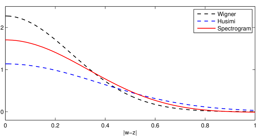
Figure 2 plots the new density μgz(w)subscript𝜇subscript𝑔𝑧𝑤\mu_{g_{z}}(w) together with the corresponding Wigner and Husimi function in terms of the distance |wz|𝑤𝑧|w-z|. Its polynomial prefactor puts the density μgzsubscript𝜇subscript𝑔𝑧\mu_{g_{z}} in between the Wigner and the Husimi Gaussian.
Refer to caption
Figure 2. Plots of the Wigner function (black dashed), the Husimi function (blue dashed), and the new density μψsubscript𝜇𝜓\mu_{\psi} (red solid) for Gaussian wave packet ψ=gz𝜓subscript𝑔𝑧\psi=g_{z} in dimension d=1𝑑1d=1 with semiclassical parameter ε=0.14𝜀0.14\varepsilon=0.14. We plot the three functions in terms of the distance |wz|𝑤𝑧|w-z|.

5.2. Gaussian superposition

Next we compute the new density μψsubscript𝜇𝜓\mu_{\psi} for a Gaussian superposition, that is, for

ψ=gz1+gz2,z1,z22d.formulae-sequence𝜓subscript𝑔subscript𝑧1subscript𝑔subscript𝑧2subscript𝑧1subscript𝑧2superscript2𝑑\psi=g_{z_{1}}+g_{z_{2}},\qquad z_{1},z_{2}\in{{\mathbb{R}}^{2d}}.

Writing the value of the Husimi function at a point z2d𝑧superscript2𝑑z\in{{\mathbb{R}}^{2d}} as

ψ(z)subscript𝜓𝑧\displaystyle{\mathcal{H}}_{\psi}(z) =(2πε)d|gz,gz1+|gz,gz2|2\displaystyle=(2\pi\varepsilon)^{-d}\left|\langle g_{z},g_{z_{1}}\rangle+|\langle g_{z},g_{z_{2}}\rangle\right|^{2}
=(2πε)d(|gz,gz1|2+|gz,gz2|2+2Re(gz1,gzgz,gz2))absentsuperscript2𝜋𝜀𝑑superscriptsubscript𝑔𝑧subscript𝑔subscript𝑧12superscriptsubscript𝑔𝑧subscript𝑔subscript𝑧222Resubscript𝑔subscript𝑧1subscript𝑔𝑧subscript𝑔𝑧subscript𝑔subscript𝑧2\displaystyle=(2\pi\varepsilon)^{-d}\;\left(|\langle g_{z},g_{z_{1}}\rangle|^{2}+|\langle g_{z},g_{z_{2}}\rangle|^{2}+2\operatorname{Re}{\left(\langle g_{z_{1}},g_{z}\rangle\langle g_{z},g_{z_{2}}\rangle\right)}\right)

motivates us to derive an explicit formula for the inner product of two Gaussian wave packets.

Lemma 5.1.

For any z1,z22dsubscript𝑧1subscript𝑧2superscript2𝑑z_{1},z_{2}\in{\mathbb{R}}^{2d}, we have

gz1,gz2=exp(|z1z2|24ε+i2εΩ(z1,z2)),subscript𝑔subscript𝑧1subscript𝑔subscript𝑧2superscriptsubscript𝑧1subscript𝑧224𝜀i2𝜀Ωsubscript𝑧1subscript𝑧2{\left\langle g_{z_{1}},g_{z_{2}}\right\rangle}=\exp{\left(-\tfrac{|z_{1}-z_{2}|^{2}}{4\varepsilon}+\tfrac{{\rm i}}{2\varepsilon}\Omega(z_{1},z_{2})\right)},

where ΩΩ\Omega is the standard symplectic form on Td2dsuperscript𝑇superscript𝑑superscript2𝑑T^{*}{\mathbb{R}}^{d}\cong{\mathbb{R}}^{2d} as defined in (2.1).

Proof.

By a direct calculation one can show

g0,gz=g0,Tzg0=exp(|z|24ε),z2d.formulae-sequencesubscript𝑔0subscript𝑔𝑧subscript𝑔0subscript𝑇𝑧subscript𝑔0superscript𝑧24𝜀𝑧superscript2𝑑{\left\langle g_{0},g_{z}\right\rangle}={\left\langle g_{0},T_{z}g_{0}\right\rangle}=\exp{\left(-\tfrac{|z|^{2}}{4\varepsilon}\right)},\qquad z\in{{\mathbb{R}}^{2d}}.

For the general case we then have

gz1,gz2subscript𝑔subscript𝑧1subscript𝑔subscript𝑧2\displaystyle{\left\langle g_{z_{1}},g_{z_{2}}\right\rangle} =Tz1g0,Tz2g0=g0,Tz1Tz2g0absentsubscript𝑇subscript𝑧1subscript𝑔0subscript𝑇subscript𝑧2subscript𝑔0subscript𝑔0subscript𝑇subscript𝑧1subscript𝑇subscript𝑧2subscript𝑔0\displaystyle={\left\langle T_{z_{1}}g_{0},T_{z_{2}}g_{0}\right\rangle}={\left\langle g_{0},T_{-z_{1}}T_{z_{2}}g_{0}\right\rangle}
=exp(i2εΩ(z1,z2))g0,Tz2z1g0=exp(i2εΩ(z1,z2)|z2z1|24ε).absenti2𝜀Ωsubscript𝑧1subscript𝑧2subscript𝑔0subscript𝑇subscript𝑧2subscript𝑧1subscript𝑔0i2𝜀Ωsubscript𝑧1subscript𝑧2superscriptsubscript𝑧2subscript𝑧124𝜀\displaystyle=\exp{\left(\tfrac{{\rm i}}{2\varepsilon}\Omega(z_{1},z_{2})\right)}{\left\langle g_{0},T_{z_{2}-z_{1}}g_{0}\right\rangle}=\exp{\left(\tfrac{{\rm i}}{2\varepsilon}\Omega(z_{1},z_{2})-\tfrac{|z_{2}-z_{1}|^{2}}{4\varepsilon}\right)}.

By Lemma 5.1 we have

gz1,gzgz,gz2=exp(|zz1|2+|zz2|24ε)exp(i2εΩ(z1z2,z))subscript𝑔subscript𝑧1subscript𝑔𝑧subscript𝑔𝑧subscript𝑔subscript𝑧2superscript𝑧subscript𝑧12superscript𝑧subscript𝑧224𝜀i2𝜀Ωsubscript𝑧1subscript𝑧2𝑧{\left\langle g_{z_{1}},g_{z}\right\rangle}{\left\langle g_{z},g_{z_{2}}\right\rangle}=\exp{\left(-\tfrac{|z-z_{1}|^{2}+|z-z_{2}|^{2}}{4\varepsilon}\right)}\exp{\left(\tfrac{{\rm i}}{2\varepsilon}\Omega(z_{1}-z_{2},z)\right)}

and obtain for the Husimi function

ψ(z)subscript𝜓𝑧\displaystyle{\mathcal{H}}_{\psi}(z) =(2πε)d(exp(|zz1|22ε)+exp(|zz2|22ε)\displaystyle=(2\pi\varepsilon)^{-d}\left(\exp{\left(-\tfrac{|z-z_{1}|^{2}}{2\varepsilon}\right)}+\exp{\left(-\tfrac{|z-z_{2}|^{2}}{2\varepsilon}\right)}\right.
+2exp(|zz1|2+|zz2|24ε)cos(12εΩ(z1z2,z))).\displaystyle\qquad\left.+2\exp{\left(-\tfrac{|z-z_{1}|^{2}+|z-z_{2}|^{2}}{4\varepsilon}\right)}\cos{\left(\tfrac{1}{2\varepsilon}\Omega(z_{1}-z_{2},z)\right)}\right).

For the Hermite spectrograms we first use Lemma 3.6 to obtain

(𝒲ψ𝒲φej)(z)subscript𝒲𝜓subscript𝒲subscript𝜑subscript𝑒𝑗𝑧\displaystyle({\mathcal{W}}_{\psi}*{\mathcal{W}}_{\varphi_{e_{j}}})(z) =(2πε)d|k=12gz,(AjTzkzj2εTzk)g0|2.absentsuperscript2𝜋𝜀𝑑superscriptsuperscriptsubscript𝑘12subscript𝑔𝑧subscript𝐴𝑗subscript𝑇subscript𝑧𝑘subscriptsuperscript𝑧𝑗2𝜀subscript𝑇subscript𝑧𝑘subscript𝑔02\displaystyle=(2\pi\varepsilon)^{-d}\;{\left|\sum_{k=1}^{2}{\left\langle g_{z},{\left(A_{j}T_{z_{k}}-\tfrac{z^{{\mathbb{C}}}_{j}}{\sqrt{2\varepsilon}}T_{z_{k}}\right)}g_{0}\right\rangle}\right|}^{2}.

We notice that, for j=1,,d𝑗1𝑑j=1,\dots,d and m=1,2𝑚12m=1,2,

AjTzm=zm,j2εTzm+TzmAj,subscript𝐴𝑗subscript𝑇subscript𝑧𝑚subscriptsuperscript𝑧𝑚𝑗2𝜀subscript𝑇subscript𝑧𝑚subscript𝑇subscript𝑧𝑚subscript𝐴𝑗A_{j}T_{z_{m}}=\tfrac{z^{{\mathbb{C}}}_{m,j}}{\sqrt{2\varepsilon}}T_{z_{m}}+T_{z_{m}}A_{j},

where zm,j:=qm,j+ipm,jz^{{\mathbb{C}}}_{m,j}\mathrel{\mathop{:}}=q_{m,j}+{\rm i}p_{m,j}\in{\mathbb{C}}. This implies that

gz,(AjTzmzj2εTzm)g0subscript𝑔𝑧subscript𝐴𝑗subscript𝑇subscript𝑧𝑚subscriptsuperscript𝑧𝑗2𝜀subscript𝑇subscript𝑧𝑚subscript𝑔0\displaystyle{\left\langle g_{z},{\left(A_{j}T_{z_{m}}-\tfrac{z^{{\mathbb{C}}}_{j}}{\sqrt{2\varepsilon}}T_{z_{m}}\right)}g_{0}\right\rangle} =gz,(zm,jzj2εTzm+TzmAj)g0absentsubscript𝑔𝑧subscriptsuperscript𝑧𝑚𝑗subscriptsuperscript𝑧𝑗2𝜀subscript𝑇subscript𝑧𝑚subscript𝑇subscript𝑧𝑚subscript𝐴𝑗subscript𝑔0\displaystyle={\left\langle g_{z},{\left(\tfrac{z^{{\mathbb{C}}}_{m,j}-z^{{\mathbb{C}}}_{j}}{\sqrt{2\varepsilon}}T_{z_{m}}+T_{z_{m}}A_{j}\right)}g_{0}\right\rangle}
=zm,jzj2εgz,gzm.absentsubscriptsuperscript𝑧𝑚𝑗subscriptsuperscript𝑧𝑗2𝜀subscript𝑔𝑧subscript𝑔subscript𝑧𝑚\displaystyle=\tfrac{z^{{\mathbb{C}}}_{m,j}-z^{{\mathbb{C}}}_{j}}{\sqrt{2\varepsilon}}{\left\langle g_{z},g_{z_{m}}\right\rangle}.

Consequently, since |zm,jzj|=|zm,jzj|subscriptsuperscript𝑧𝑚𝑗subscriptsuperscript𝑧𝑗subscript𝑧𝑚𝑗subscript𝑧𝑗|z^{{\mathbb{C}}}_{m,j}-z^{{\mathbb{C}}}_{j}|=|z_{m,j}-z_{j}| for each m𝑚m and j𝑗j, we have

(2πε)d(𝒲ψ𝒲φej)(z)superscript2𝜋𝜀𝑑subscript𝒲𝜓subscript𝒲subscript𝜑subscript𝑒𝑗𝑧\displaystyle(2\pi\varepsilon)^{d}\,({\mathcal{W}}_{\psi}*{\mathcal{W}}_{\varphi_{e_{j}}})(z) =|z1,jzj2εgz,gz1+z2,jzj2εgz,gz2|2absentsuperscriptsubscriptsuperscript𝑧1𝑗subscriptsuperscript𝑧𝑗2𝜀subscript𝑔𝑧subscript𝑔subscript𝑧1subscriptsuperscript𝑧2𝑗subscriptsuperscript𝑧𝑗2𝜀subscript𝑔𝑧subscript𝑔subscript𝑧22\displaystyle={\left|\tfrac{z^{{\mathbb{C}}}_{1,j}-z^{{\mathbb{C}}}_{j}}{\sqrt{2\varepsilon}}{\left\langle g_{z},g_{z_{1}}\right\rangle}+\tfrac{z^{{\mathbb{C}}}_{2,j}-z^{{\mathbb{C}}}_{j}}{\sqrt{2\varepsilon}}{\left\langle g_{z},g_{z_{2}}\right\rangle}\right|}^{2}
=12ε(|z1,jzj|2|gz,gz1|2+|z2,jzj|2|gz,gz2|2)absent12𝜀superscriptsubscript𝑧1𝑗subscript𝑧𝑗2superscriptsubscript𝑔𝑧subscript𝑔subscript𝑧12superscriptsubscript𝑧2𝑗subscript𝑧𝑗2superscriptsubscript𝑔𝑧subscript𝑔subscript𝑧22\displaystyle=\tfrac{1}{2\varepsilon}{\left(|z_{1,j}-z_{j}|^{2}{\left|{\left\langle g_{z},g_{z_{1}}\right\rangle}\right|}^{2}+|z_{2,j}-z_{j}|^{2}{\left|{\left\langle g_{z},g_{z_{2}}\right\rangle}\right|}^{2}\right)}
+1εRe[(z1,jzj)¯(z2,jzj)gz1,gzgz,gz2].1𝜀Re¯subscriptsuperscript𝑧1𝑗subscriptsuperscript𝑧𝑗subscriptsuperscript𝑧2𝑗subscriptsuperscript𝑧𝑗subscript𝑔subscript𝑧1subscript𝑔𝑧subscript𝑔𝑧subscript𝑔subscript𝑧2\displaystyle\quad+\tfrac{1}{\varepsilon}\operatorname{Re}{\left[\overline{(z^{{\mathbb{C}}}_{1,j}-z^{{\mathbb{C}}}_{j})}(z^{{\mathbb{C}}}_{2,j}-z^{{\mathbb{C}}}_{j}){\left\langle g_{z_{1}},g_{z}\right\rangle}{\left\langle g_{z},g_{z_{2}}\right\rangle}\right]}.

Now observe that

j=1d(z1,jzj)¯(z2,jzj)superscriptsubscript𝑗1𝑑¯subscriptsuperscript𝑧1𝑗subscriptsuperscript𝑧𝑗subscriptsuperscript𝑧2𝑗subscriptsuperscript𝑧𝑗\displaystyle\sum_{j=1}^{d}\overline{(z^{{\mathbb{C}}}_{1,j}-z^{{\mathbb{C}}}_{j})}(z^{{\mathbb{C}}}_{2,j}-z^{{\mathbb{C}}}_{j}) =j=1d[(q1,jqj)i(p1,jpj)][(q2,jqj)+i(p2,jpj)]absentsuperscriptsubscript𝑗1𝑑delimited-[]subscript𝑞1𝑗subscript𝑞𝑗isubscript𝑝1𝑗subscript𝑝𝑗delimited-[]subscript𝑞2𝑗subscript𝑞𝑗isubscript𝑝2𝑗subscript𝑝𝑗\displaystyle=\sum_{j=1}^{d}[(q_{1,j}-q_{j})-{\rm i}(p_{1,j}-p_{j})][(q_{2,j}-q_{j})+{\rm i}(p_{2,j}-p_{j})]
=(zz1)(zz2)+iΩ(zz1,zz2).absent𝑧subscript𝑧1𝑧subscript𝑧2iΩ𝑧subscript𝑧1𝑧subscript𝑧2\displaystyle=(z-z_{1})\cdot(z-z_{2})+{\rm i}\,\Omega(z-z_{1},z-z_{2}).

Therefore,

j=1d(𝒲ψ𝒲φej)(z)superscriptsubscript𝑗1𝑑subscript𝒲𝜓subscript𝒲subscript𝜑subscript𝑒𝑗𝑧\displaystyle\sum_{j=1}^{d}({\mathcal{W}}_{\psi}*{\mathcal{W}}_{\varphi_{e_{j}}})(z)
=1(2πε)d{|zz1|22εexp(|zz1|22ε)+|zz2|22εexp(|zz2|22ε)\displaystyle\quad=\tfrac{1}{(2\pi\varepsilon)^{d}}\biggl{\{}\tfrac{|z-z_{1}|^{2}}{2\varepsilon}\exp{\left(-\tfrac{|z-z_{1}|^{2}}{2\varepsilon}\right)}+\tfrac{|z-z_{2}|^{2}}{2\varepsilon}\exp{\left(-\tfrac{|z-z_{2}|^{2}}{2\varepsilon}\right)}
+1εexp(|zz1|2+|zz2|24ε)[(zz1)(zz2)cos(12εΩ(z1z2,z))\displaystyle\hskip 57.81621pt+\tfrac{1}{\varepsilon}\exp{\left(-\tfrac{|z-z_{1}|^{2}+|z-z_{2}|^{2}}{4\varepsilon}\right)}\Bigl{[}(z-z_{1})\cdot(z-z_{2})\cos{\left(\tfrac{1}{2\varepsilon}\Omega(z_{1}-z_{2},z)\right)}
Ω(zz1,zz2)sin(12εΩ(z1z2,z))]}.\displaystyle\hskip 173.44756pt-\Omega(z-z_{1},z-z_{2})\sin{\left(\tfrac{1}{2\varepsilon}\Omega(z_{1}-z_{2},z)\right)}\Bigr{]}\biggr{\}}.

Combining the Husimi function and the Hermite spectrograms gives the density μψsubscript𝜇𝜓\mu_{\psi} as plotted before in Figure 1 in the Introduction.

5.3. Hermite functions

Let us consider the higher order Hermite functions

φk:=1k!(A)kg0,k=(k1,,kd)d,\varphi_{k}\mathrel{\mathop{:}}=\frac{1}{\sqrt{k!}}(A^{\dagger})^{k}g_{0},\qquad k=(k_{1},\ldots,k_{d})\in{\mathbb{N}}^{d},

which result from the k𝑘k-fold application of the raising operator Asuperscript𝐴A^{\dagger} to the Gaussian wave packet g0subscript𝑔0g_{0} centered at the origin. The FBI transform of a Hermite function is known as

(5.2) (2πε)d/2gz,φk=1(2πε)dk!(12ε(qip))kexp(14ε|z|2)superscript2𝜋𝜀𝑑2subscript𝑔𝑧subscript𝜑𝑘1superscript2𝜋𝜀𝑑𝑘superscript12𝜀𝑞i𝑝𝑘14𝜀superscript𝑧2(2\pi\varepsilon)^{-d/2}\langle g_{z},\varphi_{k}\rangle=\frac{1}{\sqrt{(2\pi\varepsilon)^{d}k!}}\left(\tfrac{1}{\sqrt{2\varepsilon}}(q-{\rm i}p)\right)^{k}\exp\!\left(-\tfrac{1}{4\varepsilon}|z|^{2}\right)

for z2d𝑧superscript2𝑑z\in{{\mathbb{R}}^{2d}}; see [7, §2] or [17, Proposition 5]. Hence, the Husimi function satisfies

(5.3) φk(z)=1(2πε)dk!|12εz|2kexp(12ε|z|2)=j=1dhkj(zj),subscriptsubscript𝜑𝑘𝑧1superscript2𝜋𝜀𝑑𝑘superscript12𝜀𝑧2𝑘12𝜀superscript𝑧2superscriptsubscriptproduct𝑗1𝑑subscriptsubscript𝑘𝑗subscript𝑧𝑗\mathcal{H}_{\varphi_{k}}(z)=\frac{1}{(2\pi\varepsilon)^{d}k!}\left|\tfrac{1}{\sqrt{2\varepsilon}}z\right|^{2k}\,\exp\!\left(-\tfrac{1}{2\varepsilon}|z|^{2}\right)=\prod_{j=1}^{d}h_{k_{j}}(z_{j}),

where

hn(w):=φn(w),w2,h_{n}(w)\mathrel{\mathop{:}}={\mathcal{H}}_{\varphi_{n}}(w),\qquad w\in{\mathbb{R}}^{2},

denotes the Husimi function of the univariate n𝑛n-th Hermite function φnsubscript𝜑𝑛\varphi_{n}, n𝑛n\in{\mathbb{N}}. For the multivariate Hermite spectrograms we obtain the following:

Lemma 5.2.

For all kd𝑘superscript𝑑k\in{\mathbb{N}}^{d} and j=1,,d𝑗1𝑑j=1,\ldots,d and z2d𝑧superscript2𝑑z\in{{\mathbb{R}}^{2d}}, we have

(𝒲φk𝒲φej)(z)subscript𝒲subscript𝜑𝑘subscript𝒲subscript𝜑subscript𝑒𝑗𝑧\displaystyle({\mathcal{W}}_{\varphi_{k}}*{\mathcal{W}}_{\varphi_{e_{j}}})(z)
=(kjhkj1(zj)2kjhkj(zj)+(kj+1)hkj+1(zj))njhkn(zn).absentsubscript𝑘𝑗subscriptsubscript𝑘𝑗1subscript𝑧𝑗2subscript𝑘𝑗subscriptsubscript𝑘𝑗subscript𝑧𝑗subscript𝑘𝑗1subscriptsubscript𝑘𝑗1subscript𝑧𝑗subscriptproduct𝑛𝑗subscriptsubscript𝑘𝑛subscript𝑧𝑛\displaystyle\quad=\left(k_{j}h_{k_{j}-1}(z_{j})-2k_{j}h_{k_{j}}(z_{j})+(k_{j}+1)h_{k_{j}+1}(z_{j})\right)\cdot\prod_{n\neq j}h_{k_{n}}(z_{n}).
Proof.

Since Ajφk=kjφkejsubscript𝐴𝑗subscript𝜑𝑘subscript𝑘𝑗subscript𝜑𝑘subscript𝑒𝑗A_{j}\varphi_{k}=\sqrt{k_{j}}\varphi_{k-e_{j}}, Proposition 3.6 implies

(𝒲φk𝒲φej)(z)subscript𝒲subscript𝜑𝑘subscript𝒲subscript𝜑subscript𝑒𝑗𝑧\displaystyle({\mathcal{W}}_{\varphi_{k}}*{\mathcal{W}}_{\varphi_{e_{j}}})(z) =(2πε)d|gz,Ajφk12εzjgz,φk|2absentsuperscript2𝜋𝜀𝑑superscriptsubscript𝑔𝑧subscript𝐴𝑗subscript𝜑𝑘12𝜀superscriptsubscript𝑧𝑗subscript𝑔𝑧subscript𝜑𝑘2\displaystyle=(2\pi\varepsilon)^{-d}\left|\langle g_{z},A_{j}\varphi_{k}\rangle-\tfrac{1}{\sqrt{2\varepsilon}}z_{j}^{\mathbb{C}}\langle g_{z},\varphi_{k}\rangle\right|^{2}
=(2πε)d|kjgz,φkej12εzjgz,φk|2.absentsuperscript2𝜋𝜀𝑑superscriptsubscript𝑘𝑗subscript𝑔𝑧subscript𝜑𝑘subscript𝑒𝑗12𝜀superscriptsubscript𝑧𝑗subscript𝑔𝑧subscript𝜑𝑘2\displaystyle=(2\pi\varepsilon)^{-d}\left|\sqrt{k_{j}}\langle g_{z},\varphi_{k-e_{j}}\rangle-\tfrac{1}{\sqrt{2\varepsilon}}z_{j}^{\mathbb{C}}\langle g_{z},\varphi_{k}\rangle\right|^{2}.

By the formula (5.2) for the FBI transform, we obtain

(𝒲φk𝒲φej)(z)subscript𝒲subscript𝜑𝑘subscript𝒲subscript𝜑subscript𝑒𝑗𝑧\displaystyle({\mathcal{W}}_{\varphi_{k}}*{\mathcal{W}}_{\varphi_{e_{j}}})(z) =exp(12ε|z|2)(2πε)dk!|kj(12ε(qip))kej12εzj(12ε(qip))k|2absent12𝜀superscript𝑧2superscript2𝜋𝜀𝑑𝑘superscriptsubscript𝑘𝑗superscript12𝜀𝑞i𝑝𝑘subscript𝑒𝑗12𝜀superscriptsubscript𝑧𝑗superscript12𝜀𝑞i𝑝𝑘2\displaystyle=\frac{\exp\!\left(-\tfrac{1}{2\varepsilon}|z|^{2}\right)}{(2\pi\varepsilon)^{d}k!}\left|k_{j}\left(\tfrac{1}{\sqrt{2\varepsilon}}(q-{\rm i}p)\right)^{k-e_{j}}-\tfrac{1}{\sqrt{2\varepsilon}}z_{j}^{\mathbb{C}}\left(\tfrac{1}{\sqrt{2\varepsilon}}(q-{\rm i}p)\right)^{k}\right|^{2}
=exp(12ε|z|2)(2πε)dk!(kj12ε|zj|2)2|(12εz)kej|2.absent12𝜀superscript𝑧2superscript2𝜋𝜀𝑑𝑘superscriptsubscript𝑘𝑗12𝜀superscriptsubscript𝑧𝑗22superscriptsuperscript12𝜀𝑧𝑘subscript𝑒𝑗2\displaystyle=\frac{\exp\!\left(-\tfrac{1}{2\varepsilon}|z|^{2}\right)}{(2\pi\varepsilon)^{d}k!}\left(k_{j}-\tfrac{1}{2\varepsilon}|z_{j}|^{2}\right)^{2}\left|\left(\tfrac{1}{\sqrt{2\varepsilon}}z\right)^{k-e_{j}}\right|^{2}.

Then it remains to observe that

exp(12εzj2)(2πε)kj!(kj12ε|zj|2)2|12εzj|2kj212𝜀superscriptsubscript𝑧𝑗22𝜋𝜀subscript𝑘𝑗superscriptsubscript𝑘𝑗12𝜀superscriptsubscript𝑧𝑗22superscript12𝜀subscript𝑧𝑗2subscript𝑘𝑗2\displaystyle\frac{\exp\!\left(-\tfrac{1}{2\varepsilon}z_{j}^{2}\right)}{(2\pi\varepsilon)k_{j}!}\left(k_{j}-\tfrac{1}{2\varepsilon}|z_{j}|^{2}\right)^{2}\left|\tfrac{1}{\sqrt{2\varepsilon}}z_{j}\right|^{2k_{j}-2}
=kjhkj1(zj)2kjhkj(zj)+(kj+1)hkj+1(zj).absentsubscript𝑘𝑗subscriptsubscript𝑘𝑗1subscript𝑧𝑗2subscript𝑘𝑗subscriptsubscript𝑘𝑗subscript𝑧𝑗subscript𝑘𝑗1subscriptsubscript𝑘𝑗1subscript𝑧𝑗\displaystyle\qquad=k_{j}h_{k_{j}-1}(z_{j})-2k_{j}h_{k_{j}}(z_{j})+(k_{j}+1)h_{k_{j}+1}(z_{j}).

The combination of the Husimi function (5.3) and the Hermite spectrograms of Lemma 5.2 gives an explicit formula for the density μψsubscript𝜇𝜓\mu_{\psi} when ψ=φk𝜓subscript𝜑𝑘\psi=\varphi_{k} for kd𝑘superscript𝑑k\in{\mathbb{N}}^{d}.

6. Numerical Experiments

We present numerical experiments111All experiments have been performed with Matlab 8.3 on a 3.333.333.33 GHz Intel Xeon X5680 processor. for computing expectation values for the solution of the time-dependent Schrödinger equation

iεtψ(t)=(ε22Δ+V)ψ(t),ψ(0)=ψ0,formulae-sequencei𝜀subscript𝑡𝜓𝑡superscript𝜀22Δ𝑉𝜓𝑡𝜓0subscript𝜓0{\rm i}\varepsilon\partial_{t}\psi(t)=(-\tfrac{\varepsilon^{2}}{2}\Delta+V)\psi(t),\qquad\psi(0)=\psi_{0},

with three different potentials V:d:𝑉superscript𝑑V:{\mathbb{R}}^{d}\to{\mathbb{R}}. The various setups shall illustrate important aspects of our new algorithm, such as the second order accuracy with respect to ε𝜀\varepsilon, the good applicability in higher dimensions, and the capability of describing fundamental quantum effects.

6.1. Discretization

For the algorithmic discretization of Corollary 4.1 we proceed similarly as in [16, 10, 14]. We consider various smooth functions a:2d:𝑎superscript2𝑑a:{{\mathbb{R}}^{2d}}\to{\mathbb{R}} and evaluate the phase space integral on the right hand side of the semiclassical approximation

ψ(t),op(a)ψ(t)𝜓𝑡op𝑎𝜓𝑡\displaystyle\left\langle\psi(t),\operatorname{op}(a)\psi(t)\right\rangle =2d(aΦt)(z)μψ0(z)dz+O(ε2)absentsubscriptsuperscript2𝑑𝑎subscriptΦ𝑡𝑧subscript𝜇subscript𝜓0𝑧differential-d𝑧𝑂superscript𝜀2\displaystyle=\int_{{\mathbb{R}}^{2d}}(a\circ\Phi_{t})(z)\mu_{\psi_{0}}(z){\rm d}z+O(\varepsilon^{2})

for normalized initial data ψ0L2(d)subscript𝜓0superscript𝐿2superscript𝑑\psi_{0}\in L^{2}({\mathbb{R}}^{d}), ψ0=1normsubscript𝜓01\|\psi_{0}\|=1, via the quadrature formula

2d(aΦt)(z)μψ0(z)dzsubscriptsuperscript2𝑑𝑎subscriptΦ𝑡𝑧subscript𝜇subscript𝜓0𝑧differential-d𝑧\displaystyle\int_{{\mathbb{R}}^{2d}}(a\circ\Phi_{t})(z)\mu_{\psi_{0}}(z){\rm d}z =(1+d2)2d(aΦt)(z)ψ0(z)dzabsent1𝑑2subscriptsuperscript2𝑑𝑎subscriptΦ𝑡𝑧subscriptsubscript𝜓0𝑧differential-d𝑧\displaystyle=(1+\tfrac{d}{2})\int_{{\mathbb{R}}^{2d}}(a\circ\Phi_{t})(z){\mathcal{H}}_{\psi_{0}}(z){\rm d}z
12j=1d2d(aΦt)(z)(𝒲ψ0𝒲φej)(z)dz12superscriptsubscript𝑗1𝑑subscriptsuperscript2𝑑𝑎subscriptΦ𝑡𝑧subscript𝒲subscript𝜓0subscript𝒲subscript𝜑subscript𝑒𝑗𝑧differential-d𝑧\displaystyle\quad-\tfrac{1}{2}\sum_{j=1}^{d}\int_{{\mathbb{R}}^{2d}}(a\circ\Phi_{t})(z)({\mathcal{W}}_{\psi_{0}}*{\mathcal{W}}_{\varphi_{e_{j}}})(z){\rm d}z
1+d2Nk=1N(aΦt)(zk)d2Nk=1N(aΦt)(wk),absent1𝑑2𝑁superscriptsubscript𝑘1𝑁𝑎subscriptΦ𝑡subscript𝑧𝑘𝑑2𝑁superscriptsubscript𝑘1𝑁𝑎subscriptΦ𝑡subscript𝑤𝑘\displaystyle\approx\frac{1+\tfrac{d}{2}}{N}\sum_{k=1}^{N}(a\circ\Phi_{t})(z_{k})-\frac{d}{2N}\sum_{k=1}^{N}(a\circ\Phi_{t})(w_{k}),

where one samples the quadrature points according to the probability measures

z1,,zNψ0,w1,,wN1dj=1d𝒲ψ0𝒲φej;formulae-sequencesimilar-tosubscript𝑧1subscript𝑧𝑁subscriptsubscript𝜓0similar-tosubscript𝑤1subscript𝑤𝑁1𝑑superscriptsubscript𝑗1𝑑subscript𝒲subscript𝜓0subscript𝒲subscript𝜑subscript𝑒𝑗z_{1},\ldots,z_{N}\sim{\mathcal{H}}_{\psi_{0}}\,,\qquad w_{1},\ldots,w_{N}\sim\tfrac{1}{d}\sum_{j=1}^{d}{\mathcal{W}}_{\psi_{0}}*{\mathcal{W}}_{\varphi_{e_{j}}};

see also §A for the sampling strategies used for the Hermite spectrograms. The rate of convergence for the above quadrature rule is proportional to N1/2superscript𝑁12N^{-1/2} for Monte Carlo samplings. For low discrepancy (Quasi-Monte Carlo) sampling the convergence is faster, that is, of the order log(N)2d/N\log(N)^{2d}/N. However, the literature on non-uniform Quasi-Monte Carlo sampling is scarce, and it seems to be an open question whether the transformed Halton sequences employed in our numerical experiments form indeed a low discrepancy set or just come very close to being so in practice, see also [1].

For the discretization of the Hamiltonian flow ΦtsubscriptΦ𝑡\Phi_{t}, we apply the eighth-order symplectic splitting method from [27, Table 2.D], which is a suitable composition of the linear flows of

{q˙=pp˙=0 and {q˙=0p˙=V(q).cases˙𝑞𝑝otherwise˙𝑝0otherwise and cases˙𝑞0otherwise˙𝑝𝑉𝑞otherwise\begin{cases}\dot{q}=p\\ \dot{p}=0\end{cases}\qquad\text{ and }\qquad\begin{cases}\dot{q}=0\\ \dot{p}=-\nabla V(q)\end{cases}.

Since our algorithm evolves an ensemble of classical trajectories, the use of symplectic time integrators is crucial; see also [16, Fig. 4.2].
Refer to caption
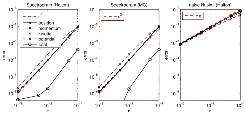
Figure 3. Average errors (6.2) of the expectation values of various observables on the time interval [0,20]020[0,20] for the new spectrogram method with initial Halton (left) and Monte Carlo (middle) sampling and results for the naive Husimi method with Halton sampling (right) for the torsional potential and Gaussian initial data centered at z=(1,0,0,0)𝑧1000z=(1,0,0,0).

6.2. Two-dimensional torsional potential

Our first numerical experiments are conducted for the two-dimensional torsional potential

V(q1,q2)=2cos(q1)cos(q2),q2,formulae-sequence𝑉subscript𝑞1subscript𝑞22subscript𝑞1subscript𝑞2𝑞superscript2V(q_{1},q_{2})=2-\cos(q_{1})-\cos(q_{2}),\qquad q\in{\mathbb{R}}^{2},

and different values of the semiclassical parameter ε𝜀\varepsilon. As the initial state we consider the Gaussian wave packet ψ0=gzsubscript𝜓0subscript𝑔𝑧\psi_{0}=g_{z} with phase space center z=(1,0,0,0)𝑧1000z=(1,0,0,0). This setup has already been considered in [5, 16, 14, 10]. We investigate the dynamics of the following symbols a:4:𝑎superscript4a:{\mathbb{R}}^{4}\to{\mathbb{R}},

  1. (1)

    Position: a(q,p)=q1𝑎𝑞𝑝subscript𝑞1a(q,p)=q_{1} and a(q,p)=q2𝑎𝑞𝑝subscript𝑞2a(q,p)=q_{2},

  2. (2)

    Momentum: a(q,p)=p1𝑎𝑞𝑝subscript𝑝1a(q,p)=p_{1} and a(q,p)=p2𝑎𝑞𝑝subscript𝑝2a(q,p)=p_{2},

  3. (3)

    Kinetic and potential energy: a(q,p)=12|p|2𝑎𝑞𝑝12superscript𝑝2a(q,p)=\tfrac{1}{2}|p|^{2} and a(q,p)=V(q)𝑎𝑞𝑝𝑉𝑞a(q,p)=V(q),

  4. (4)

    Total energy: a(q,p)=12|p|2+V(q)𝑎𝑞𝑝12superscript𝑝2𝑉𝑞a(q,p)=\tfrac{1}{2}|p|^{2}+V(q),

and compare the outcome of the new algorithm with the naive, first-order Husimi approximation

(6.1) ψ(t),op(a)ψ(t)=2d(aΦt)(z)ψ0(z)dz+O(ε).𝜓𝑡op𝑎𝜓𝑡subscriptsuperscript2𝑑𝑎subscriptΦ𝑡𝑧subscriptsubscript𝜓0𝑧differential-d𝑧𝑂𝜀\langle\psi(t),\operatorname{op}(a)\psi(t)\rangle=\int_{{{\mathbb{R}}^{2d}}}(a\circ\Phi_{t})(z){\mathcal{H}}_{\psi_{0}}(z){\rm d}z+O(\varepsilon).

The left and middle panel of Figure 3 confirm the second order accuracy of the new method for both Monte Carlo and Halton type samplings of the initial density μψ0subscript𝜇subscript𝜓0\mu_{\psi_{0}}. The right panel illustrates that the naive Husimi method is indeed only of first order in ε𝜀\varepsilon. The time-averaged errors

(6.2) 120020|ψref(t),op(a)ψref(t)1+d2Nk=1N(aΦt)(zk)+d2Nk=1N(aΦt)(wk)|dt120superscriptsubscript020subscript𝜓ref𝑡op𝑎subscript𝜓ref𝑡1𝑑2𝑁superscriptsubscript𝑘1𝑁𝑎subscriptΦ𝑡subscript𝑧𝑘𝑑2𝑁superscriptsubscript𝑘1𝑁𝑎subscriptΦ𝑡subscript𝑤𝑘differential-d𝑡\frac{1}{20}\int_{0}^{20}\Big{|}\langle\psi_{\rm ref}(t),\operatorname{op}(a)\psi_{\rm ref}(t)\rangle-\frac{1+\tfrac{d}{2}}{N}\sum_{k=1}^{N}(a\circ\Phi_{t})(z_{k})+\frac{d}{2N}\sum_{k=1}^{N}(a\circ\Phi_{t})(w_{k})\Big{|}{\rm d}t

are taken with respect to highly accurate grid based reference solutions ψref(t)ψ(t)subscript𝜓ref𝑡𝜓𝑡\psi_{\rm ref}(t)\approx\psi(t) of the Schrödinger equation; for details see Appendix B.1.

The total energy error in Figure 3 is smaller than the errors for other expectation values. Firstly, this can be explained by the fact that the total energy error is time independent, as explained in Remark 4.3, and symplectic integrators are practically energy preserving on the time scales considered here. Secondly, the leading O(ε2)𝑂superscript𝜀2O(\varepsilon^{2}) term in the asymptotic expansion of the error

\displaystyle\langle gz,op(h)gz2dh(w)μgz(w)dw=2dh(w)(𝒲gz(1ε4Δ)gz)(w)dw\displaystyle g_{z},\operatorname{op}(h)g_{z}\rangle-\int_{{\mathbb{R}}^{2d}}h(w)\mu_{g_{z}}(w)dw=\int_{{\mathbb{R}}^{2d}}h(w)({\mathcal{W}}_{g_{z}}-(1-\tfrac{\varepsilon}{4}\Delta){\mathcal{H}}_{g_{z}})(w)dw
=2dh(w)(𝒲gz(1ε4Δ)(1+ε4Δ+ε232Δ2)𝒲gz)(w)𝑑w+O(ε3)absentsubscriptsuperscript2𝑑𝑤subscript𝒲subscript𝑔𝑧1𝜀4Δ1𝜀4Δsuperscript𝜀232superscriptΔ2subscript𝒲subscript𝑔𝑧𝑤differential-d𝑤𝑂superscript𝜀3\displaystyle=\int_{{\mathbb{R}}^{2d}}h(w)\left({\mathcal{W}}_{g_{z}}-(1-\tfrac{\varepsilon}{4}\Delta)(1+\tfrac{\varepsilon}{4}\Delta+\tfrac{\varepsilon^{2}}{32}\Delta^{2}){\mathcal{W}}_{g_{z}}\right)(w)dw+O(\varepsilon^{3})
=ε2322dh(w)Δ2𝒲gz(w)𝑑w+O(ε3)absentsuperscript𝜀232subscriptsuperscript2𝑑𝑤superscriptΔ2subscript𝒲subscript𝑔𝑧𝑤differential-d𝑤𝑂superscript𝜀3\displaystyle=\tfrac{\varepsilon^{2}}{32}\int_{{\mathbb{R}}^{2d}}h(w)\Delta^{2}{\mathcal{W}}_{g_{z}}(w)dw+O(\varepsilon^{3})

can be bounded by the small constant

|1322dΔ2h(w)𝒲gz(w)𝑑w|116,132subscriptsuperscript2𝑑superscriptΔ2𝑤subscript𝒲subscript𝑔𝑧𝑤differential-d𝑤116\displaystyle\big{|}\tfrac{1}{32}\int_{{\mathbb{R}}^{2d}}\Delta^{2}h(w){\mathcal{W}}_{g_{z}}(w)dw\big{|}\leq\tfrac{1}{16},

which follows from the special form of the torsional potential and the initial state. The total energy errors for small values of ε𝜀\varepsilon are larger in the left panel of Figure 3 than in the middle panel, since the relatively small number of Halton points gives rise to perceptible quadrature errors.
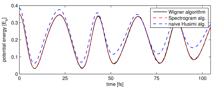
Refer to caption
Figure 4. The approximate dynamics of the potential energies for the 323232-dimensional Henon–Heiles system obtained by the Wigner, Spectrogram, and naive Husimi algorithms.

6.3. Henon–Heiles dynamics for 𝒅=𝟑𝟐𝒅32d=32

Henon–Heiles type systems have been used for benchmark simulations with the multiconfiguration time-dependent Hartree method (MCTDH); see [22]. We follow the presentation in [15, §5.B] by using the potential

V32(q)=12|q|2+1.8436j=131(qj2qj+113qj+13)+0.4j=131(qj2+qj+12)2subscript𝑉32𝑞12superscript𝑞21.8436superscriptsubscript𝑗131superscriptsubscript𝑞𝑗2subscript𝑞𝑗113superscriptsubscript𝑞𝑗130.4superscriptsubscript𝑗131superscriptsuperscriptsubscript𝑞𝑗2superscriptsubscript𝑞𝑗122V_{32}(q)=\tfrac{1}{2}|q|^{2}+1.8436\sum_{j=1}^{31}(q_{j}^{2}q_{j+1}-\tfrac{1}{3}q_{j+1}^{3})+0.4\sum_{j=1}^{31}(q_{j}^{2}+q_{j+1}^{2})^{2}

and the semiclassical parameter ε=0.0029𝜀0.0029\varepsilon=0.0029, which is a model for the dynamics of a hydrogen atom on a high-dimensional potential energy surface that exhibits regions of chaotic motion. The quartic confinement guarantees that none of the classical trajectories escapes to infinity. Moreover, as in [22, 15], the initial state is a Gaussian wave packet ψ0=gzsubscript𝜓0subscript𝑔𝑧\psi_{0}=g_{z} centered at z=(q,p)𝑧𝑞𝑝z=(q,p) with p=0𝑝0p=0 and qj=0.1215subscript𝑞𝑗0.1215q_{j}=0.1215 for all j=1,,32𝑗132j=1,\ldots,32.

Since grid-based reference solutions are not available for this high-dimensional setting, we compare our method with the results obtained by the second order approximation

ψ(t),op(a)ψ(t)=2d(aΦt)(z)𝒲ψ0(z)dz+O(ε2).𝜓𝑡op𝑎𝜓𝑡subscriptsuperscript2𝑑𝑎subscriptΦ𝑡𝑧subscript𝒲subscript𝜓0𝑧differential-d𝑧𝑂superscript𝜀2\langle\psi(t),\operatorname{op}(a)\psi(t)\rangle=\int_{{{\mathbb{R}}^{2d}}}(a\circ\Phi_{t})(z){\mathcal{W}}_{\psi_{0}}(z){\rm d}z+O(\varepsilon^{2}).

Note that, in this particular case, the initial Wigner function 𝒲ψ0(z)subscript𝒲subscript𝜓0𝑧{\mathcal{W}}_{\psi_{0}}(z) is the Gaussian (5.1), and hence the Wigner algorithm does not pose a difficulty in the initial sampling. Figure 4 shows the good agreement of the results from the Wigner and the spectrogram methods by means of the potential energy, and a considerable discrepancy with respect to the naive Husimi approximation (6.1).

6.4. Escape from a cubic potential well

Finally, we explore whether the new method is capable of describing the evolution of a quantum system that moves out of a potential well. For this purpose we consider the semiclassical Schrödinger operator H=ε22Δ+V𝐻superscript𝜀22Δ𝑉H=-\tfrac{\varepsilon^{2}}{2}\Delta+V with the one-dimensional barrier potential

V(q)=2.328q2+q3+0.025q4,q,formulae-sequence𝑉𝑞2.328superscript𝑞2superscript𝑞30.025superscript𝑞4𝑞V(q)=2.328\cdot q^{2}+q^{3}+0.025q^{4},\qquad q\in{\mathbb{R}},

and ε=0.4642𝜀0.4642\varepsilon=0.4642; see also Figure 5. This Hamiltonian can be derived from the Schrödinger operator

122Δ+12x2+0.1x312superscriptPlanck-constant-over-2-pi2Δ12superscript𝑥20.1superscript𝑥3-\tfrac{1}{2}\hbar^{2}\Delta+\tfrac{1}{2}x^{2}+0.1x^{3}

with =1Planck-constant-over-2-pi1\hbar=1 from [23, 24] by applying the space rescaling x0.13xmaps-to𝑥30.1𝑥x\mapsto\sqrt[3]{0.1}x and adding the confinement term 0.025q40.025superscript𝑞40.025\cdot q^{4}. The confinement prevents phase space trajectories from finite time blow up and guarantees that H𝐻H is essentially self-adjoint. The global potential energy minimum V(xglob)4765𝑉subscript𝑥glob4765V(x_{\rm glob})\approx-4765 is attained at xglob28.4subscript𝑥glob28.4x_{\rm glob}\approx-28.4, and the confinement is very small in the region of interest close to the origin.

Refer to caption
Figure 5. The cubic barrier potential V𝑉V with the barrier energy Vbsubscript𝑉𝑏V_{b} and the energy h(z0)subscript𝑧0h(z_{0}) of the trapped classical particle.

As initial states we consider translated Hermite functions

ψ0=Tz0φk,k{0,1,3,6}formulae-sequencesubscript𝜓0subscript𝑇subscript𝑧0subscript𝜑𝑘𝑘0136\psi_{0}=T_{z_{0}}\varphi_{k},\qquad k\in\{0,1,3,6\}

localized around z0=(0.4642,1)subscript𝑧00.46421z_{0}=(0.4642,-1), which corresponds to the initial phase space center used in [23]. Since the associated classical energy h(z0)subscript𝑧0h(z_{0}) lies below the barrier energy Vb2.03subscript𝑉𝑏2.03V_{b}\approx 2.03, the classical particle is trapped in the well for all times. In contrast, the quantum energy of the initial state gz0subscript𝑔subscript𝑧0g_{z_{0}} is approximately 2.092.092.09, and the energies of the excited states are even higher. Consequently, the expected phase space center of the quantum particle will escape from the classical trapping region after short time.

Figure 6 displays the trajectories of the expected phase space centers obtained by the purely classical, the full quantum, and the semiclassical spectrogram dynamics for the four different initial states. The results from the spectrogram algorithm show decent qualitative agreement with the behavior of the quantum solution even though the semiclassical parameter ε=0.4642𝜀0.4642\varepsilon=0.4642 is rather large. We also note that the results become more accurate for initial states of higher energy.
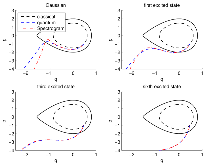
Refer to caption
Figure 6. Trajectories of the expected phase space centers obtained from quantum references and the new spectrogram algorithm for different initial states ψ0=Tz0φksubscript𝜓0subscript𝑇subscript𝑧0subscript𝜑𝑘\psi_{0}=T_{z_{0}}\varphi_{k}. The dashed black line shows the periodic classical orbit associated with z0subscript𝑧0z_{0}, and the solid black line illustrates the border of the trapping region.

The spectrogram algorithm is also capable of describing the evolution of the probability that the quantum particle escapes the potential well and is found in the region (,xmax]subscript𝑥max(-\infty,x_{\rm max}], where xmax1.62subscript𝑥max1.62x_{\rm max}\approx-1.62 is the local maximum of the barrier potential. To illustrate this property, we introduce the approximate escape probability

P(t)=ψt,op(r)ψtψtχ(,xmax]L22𝑃𝑡subscript𝜓𝑡op𝑟subscript𝜓𝑡subscriptsuperscriptnormsubscript𝜓𝑡subscript𝜒subscript𝑥max2superscript𝐿2P(t)=\left\langle\psi_{t},\operatorname{op}(r)\psi_{t}\right\rangle\approx\|\psi_{t}\chi_{(-\infty,x_{\rm max}]}\|^{2}_{L^{2}}

with the smooth symbol r(q,p)=exp(0.01/(qxmax)2)χ(,xmax](q)𝑟𝑞𝑝0.01superscript𝑞subscript𝑥max2subscript𝜒subscript𝑥max𝑞r(q,p)=\exp(-0.01/(q-x_{\rm max})^{2})\chi_{(-\infty,x_{\rm max}]}(q), where χAsubscript𝜒𝐴\chi_{A} denotes the characteristic function of the set A𝐴A. P(t)𝑃𝑡P(t) can easily be approximated by the spectrogram algorithm, and accurate numerical references are available; see Appendix B.3.
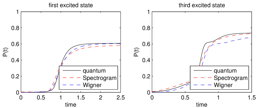
Refer to caption
Figure 7. Approximate escape probabilities P(t)𝑃𝑡P(t) computed from a highly accurate numerical quantum reference, and results of the spectrogram and Wigner algorithms for the initial states Tz0φ1subscript𝑇subscript𝑧0subscript𝜑1T_{z_{0}}\varphi_{1}, and Tz0φ3subscript𝑇subscript𝑧0subscript𝜑3T_{z_{0}}\varphi_{3}.

Figure 7 shows by means of two different initial states that the spectrogram algorithm yields a good qualitative picture of the evolution of escape probabilities.

Appendix A Sampling by the Gamma distribution

A.1. Using the Gamma distribution

We consider the Hermite functions translated by the Heisenberg–Weyl operator,

ψ=Tzφk,kd,z2d.formulae-sequence𝜓subscript𝑇𝑧subscript𝜑𝑘formulae-sequence𝑘superscript𝑑𝑧superscript2𝑑\psi=T_{z}\varphi_{k},\qquad k\in{\mathbb{N}}^{d},\qquad z\in{\mathbb{R}}^{2d}.

Then, by the covariance property (2.6), the Hermite spectrogram takes the form

(𝒲Tzφk𝒲φej)(w)=(𝒲φk𝒲φej)(wz),w2d,formulae-sequencesubscript𝒲subscript𝑇𝑧subscript𝜑𝑘subscript𝒲subscript𝜑subscript𝑒𝑗𝑤subscript𝒲subscript𝜑𝑘subscript𝒲subscript𝜑subscript𝑒𝑗𝑤𝑧𝑤superscript2𝑑({\mathcal{W}}_{T_{z}\varphi_{k}}*{\mathcal{W}}_{\varphi_{e_{j}}})(w)=({\mathcal{W}}_{\varphi_{k}}*{\mathcal{W}}_{\varphi_{e_{j}}})(w-z),\qquad w\in{{\mathbb{R}}^{2d}},

and by Lemma 5.2, we only have to consider the two-dimensional probability densities

wjhn(wjzj)=12πεn!|12ε(wjzj)|2nexp(12ε|wjzj|2)maps-tosubscript𝑤𝑗subscript𝑛subscript𝑤𝑗subscript𝑧𝑗12𝜋𝜀𝑛superscript12𝜀subscript𝑤𝑗subscript𝑧𝑗2𝑛12𝜀superscriptsubscript𝑤𝑗subscript𝑧𝑗2w_{j}\mapsto h_{n}(w_{j}-z_{j})=\frac{1}{2\pi\varepsilon\cdot n!}\left|\tfrac{1}{\sqrt{2\varepsilon}}(w_{j}-z_{j})\right|^{2n}\exp\!\left(-\tfrac{1}{2\varepsilon}|w_{j}-z_{j}|^{2}\right)

with n{k1,,kd}𝑛subscript𝑘1subscript𝑘𝑑n\in\{k_{1},\ldots,k_{d}\}. Specifically, we first translate by zjsubscript𝑧𝑗-z_{j} and then use the uniform distribution on [0,2π]02𝜋[0,2\pi] for the angular part combined with sampling from

rr2n+12nεn+1n!exp(12εr2)maps-to𝑟superscript𝑟2𝑛1superscript2𝑛superscript𝜀𝑛1𝑛12𝜀superscript𝑟2r\mapsto\frac{r^{2n+1}}{2^{n}\varepsilon^{n+1}n!}\exp\!\left(-\tfrac{1}{2\varepsilon}r^{2}\right)

for the radial part. Since

abr2n+12nεn+1n!exp(12εr2)dr=a2b2τn(2ε)n+1n!exp(12ετ)dτsuperscriptsubscript𝑎𝑏superscript𝑟2𝑛1superscript2𝑛superscript𝜀𝑛1𝑛12𝜀superscript𝑟2differential-d𝑟superscriptsubscriptsuperscript𝑎2superscript𝑏2superscript𝜏𝑛superscript2𝜀𝑛1𝑛12𝜀𝜏differential-d𝜏\int_{a}^{b}\frac{r^{2n+1}}{2^{n}\varepsilon^{n+1}n!}\exp\!\left(-\tfrac{1}{2\varepsilon}r^{2}\right){\rm d}r=\int_{a^{2}}^{b^{2}}\frac{\tau^{n}}{(2\varepsilon)^{n+1}n!}\exp\!\left(-\tfrac{1}{2\varepsilon}\tau\right){\rm d}\tau

for all a,b>0𝑎𝑏0a,b>0, we use the Gamma distribution with parameters n+1𝑛1n+1 and 2ε2𝜀2\varepsilon for the radial sampling.

In the particular case k=0𝑘0k=0, φ0=g0subscript𝜑0subscript𝑔0\varphi_{0}=g_{0} and so Tzφ0=gzsubscript𝑇𝑧subscript𝜑0subscript𝑔𝑧T_{z}\varphi_{0}=g_{z} is a Gaussian wave packet and

μgz(w)=(2πε)d(1+d214ε|wz|2)exp(12ε|wz|2),w2d;formulae-sequencesubscript𝜇subscript𝑔𝑧𝑤superscript2𝜋𝜀𝑑1𝑑214𝜀superscript𝑤𝑧212𝜀superscript𝑤𝑧2𝑤superscript2𝑑\mu_{g_{z}}(w)=(2\pi\varepsilon)^{-d}\left(1+\tfrac{d}{2}-\tfrac{1}{4\varepsilon}|w-z|^{2}\right)\exp\!\left(-\tfrac{1}{2\varepsilon}|w-z|^{2}\right),\qquad w\in{{\mathbb{R}}^{2d}};

see §5.1. One can directly sample this 2d2𝑑2d-dimensional probability density without factorizing its summands. After translation by z𝑧-z, one decomposes into a radial part and an independent angular variable which is uniformly distributed on 𝕊2d1superscript𝕊2𝑑1\mathbb{S}^{2d-1}. The radial density is given by

rrd(2ε)d+1d!exp(r/2ε),maps-to𝑟superscript𝑟𝑑superscript2𝜀𝑑1𝑑𝑟2𝜀r\mapsto\frac{r^{d}}{(2\varepsilon)^{d+1}d!}\exp\!\left(-r/2\varepsilon\right),

which corresponds to a Gamma distribution with parameters d+1𝑑1d+1 and 2ε2𝜀2\varepsilon.

A.2. Monte Carlo sampling

Pseudorandom numbers uniformly distributed on a multi-dimensional unit sphere are obtained by sampling from multivariate normal distributions and subsequent normalization, while Gamma distributed pseudorandom samples only require the uniform distribution on the unit cube together with the (numerical) inverse of the cumulative Gamma distribution function. Hence a Monte-Carlo sampling of μTzφksubscript𝜇subscript𝑇𝑧subscript𝜑𝑘\mu_{T_{z}\varphi_{k}} is straightforward.

A.3. Quasi-Monte Carlo sampling

For the generation of Quasi-Monte Carlo points we have heuristically mimicked the Monte-Carlo procedure of §A.2 by replacing the pseudorandom samples from the uniform distribution on the unit cube by a Halton sequence. Whether the resulting points are of low discrepancy with respect to the distribution μTzφksubscript𝜇subscript𝑇𝑧subscript𝜑𝑘\mu_{T_{z}\varphi_{k}} seems to be an open question not answered by the current literature, see e.g. [1].

Appendix B Numerical data

B.1. Two-dimensional torsional system

Table 1 contains the number of initial sampling points and the computational time for the new spectrogram algorithm. In the case of Monte Carlo integration, the results in Figure 3 are averaged over ten independent runs. For the time propagation we apply the above mentioned eighth-order symplectic integrator with time stepping 101superscript10110^{-1}. The parameters of the grid-based reference solver are collected in Table 2.

ε𝜀\varepsilon MC points comp. time Halton points comp. time
101superscript10110^{-1} 51045superscript1045\cdot 10^{4} 23s 51045superscript1045\cdot 10^{4} 16s
51025superscript1025\cdot 10^{-2} 31053superscript1053\cdot 10^{5} 1m59s 105superscript10510^{5} 33s
102superscript10210^{-2} 61056superscript1056\cdot 10^{5} 7m16s 21052superscript1052\cdot 10^{5} 1m59s
51035superscript1035\cdot 10^{-3} 1.51061.5superscript1061.5\cdot 10^{6} 14m15s 81058superscript1058\cdot 10^{5} 6m50s
103superscript10310^{-3} 1010610superscript10610\cdot 10^{6} 68m30s 21062superscript1062\cdot 10^{6} 18m31s
Table 1. Computational data for the execution of the new spectrogram algorithm for the two dimensional torsional potential and Gaussian initial data on the time interval [0,20]020[0,20]. The computation times are for one run only. They scale linearly with respect to the number of initial sampling points.
ε𝜀\varepsilon ##\#timesteps comp. domain space grid
101superscript10110^{-1} 51035superscript1035\cdot 10^{3} [3,3]×[3,3]3333[-3,3]\times[-3,3] 1536×1536153615361536\times 1536
51025superscript1025\cdot 10^{-2} 51035superscript1035\cdot 10^{3} [3,3]×[3,3]3333[-3,3]\times[-3,3] 1536×1536153615361536\times 1536
102superscript10210^{-2} 7.51037.5superscript1037.5\cdot 10^{3} [2,2]×[2,2]2222[-2,2]\times[-2,2] 2048×2048204820482048\times 2048
51035superscript1035\cdot 10^{-3} 104superscript10410^{4} [2,2]×[2,2]2222[-2,2]\times[-2,2] 2048×2048204820482048\times 2048
103superscript10310^{-3} 104superscript10410^{4} [2,2]×[2,2]2222[-2,2]\times[-2,2] 2048×2048204820482048\times 2048
Table 2. Parameters of the grid-based reference solutions for the two-dimensional torsional potential. The discretization has been done by Fourier collocation in 2superscript2{\mathbb{R}}^{2} and Strang splitting in time.

B.2. Henon–Heiles system for 𝒅=𝟑𝟐𝒅32d=32

For the initial sampling we used 217superscript2172^{17} Halton type points for all three initial densities, that is, the Wigner and the Husimi functions and the new density μψ0subscript𝜇subscript𝜓0\mu_{\psi_{0}}. The time stepping of the eighth order time integrator is 21022superscript1022\cdot 10^{-2}.

B.3. One-dimensional cubic well

For the spectrogram algorithm we employed 214superscript2142^{14} Halton points and the eighth-order integrator with time stepping 102superscript10210^{-2}, which results in a computational time of 222 seconds. The quantum references are generated by means of a Strang splitting with 215superscript2152^{15} Fourier modes on the interval [40,4]404[-40,4].

References

  • [1] C. Aistleitner and J. Dick, Low-discrepancy point sets for non-uniform measures, Acta Arith., 163 (2014), pp. 345–369.
  • [2] A. G. Athanassoulis, N. J. Mauser, and T. Paul, Coarse-scale representations and smoothed Wigner transforms, J. Math. Pures Appl. (9), 91 (2009), pp. 296–338.
  • [3] A. Bouzouina and D. Robert, Uniform semiclassical estimates for the propagation of quantum observables, Duke Math. J., 111 (2002), pp. 223–252.
  • [4] M. A. de Gosson, Symplectic Methods in Harmonic Analysis and in Mathematical Physics, Pseudo-Differential Operators, Springer, 2011.
  • [5] E. Faou, V. Gradinaru, and C. Lubich, Computing semiclassical quantum dynamics with Hagedorn wavepackets, SIAM J. Sci. Comput., 31 (2009), pp. 3027–3041.
  • [6] P. Flandrin, Time-frequency/time-scale analysis, vol. 10 of Wavelet Analysis and its Applications, Academic Press, Inc., San Diego, CA, 1999. With a preface by Yves Meyer, Translated from the French by Joachim Stöckler.
  • [7]  , A note on reassigned Gabor spectrograms of Hermite functions, J. Fourier Anal. Appl., 19 (2013), pp. 285–295.
  • [8]  , Time-frequency filtering based on spectrogram zeros, 2015. HAL preprint ensl-01121522.
  • [9] G. B. Folland, Harmonic analysis in phase space, vol. 122 of Annals of Mathematics Studies, Princeton University Press, Princeton, NJ, 1989.
  • [10] W. Gaim and C. Lasser, Corrections to Wigner type phase space methods, Nonlinearity, 27 (2014), pp. 2951–2974.
  • [11] P. Gérard, P. A. Markowich, N. J. Mauser, and F. Poupaud, Homogenization limits and Wigner transforms, Comm. Pure Appl. Math., 50 (1997), pp. 323–379.
  • [12] A. J. E. M. Janssen, Positivity and spread of bilinear time-frequency distributions, in The Wigner distribution, Elsevier, Amsterdam, 1997, pp. 1–58.
  • [13] J. Keller, Quantum Dynamics on Potential Energy Surfaces — Simpler States and Simpler Dynamics, PhD thesis, Technische Universität München, 2015.
  • [14] J. Keller and C. Lasser, Propagation of quantum expectations with Husimi functions, SIAM Journal on Applied Mathematics, 73 (2013), pp. 1557–1581.
  • [15]  , Quasi-classical description of molecular dynamics based on Egorov’s theorem, The Journal of Chemical Physics, 141 (2014), p. 054104.
  • [16] C. Lasser and S. Röblitz, Computing expectation values for molecular quantum dynamics, SIAM Journal on Scientific Computing, 32 (2010), pp. 1465–1483.
  • [17] C. Lasser and S. Troppmann, Hagedorn wavepackets in time-frequency and phase space, J. Fourier An. Appl., (2014), pp. 1–36.
  • [18] N. Lerner, Metrics on the phase space and non-selfadjoint pseudo-differential operators, vol. 3 of Pseudo-Differential Operators. Theory and Applications, Birkhäuser Verlag, Basel, 2010.
  • [19] P.-L. Lions and T. Paul, Sur les mesures de Wigner, Rev. Mat. Iberoamericana, 9 (1993), pp. 553–618.
  • [20] P. Loughlin, J. Pitton, and B. Hannaford, Approximating time-frequency density functions via optimal combinations of spectrograms, Signal Processing Letters, IEEE, 1 (1994), pp. 199–202.
  • [21] A. Martinez, An introduction to semiclassical and microlocal analysis, Universitext, Springer-Verlag, New York, 2002.
  • [22] M. Nest and H.-D. Meyer, Benchmark calculations on high-dimensional Henon-Heiles potentials with the multi-configuration time dependent Hartree (MCTDH) method, J. Chem. Phys., 117 (2002), pp. 10499–10505.
  • [23] T. Ohsawa and M. Leok, Symplectic semiclassical wave packet dynamics, J. Phys. A, 46 (2013), pp. 405201, 28.
  • [24] O. V. Prezhdo and Y. V. Pereverzev, Quantized Hamilton dynamics, The Journal of Chemical Physics, 113 (2000).
  • [25] D. Robert, Autour de l’approximation semi-classique, no. 68, Birkhauser, 1987.
  • [26] F. Soto and P. Claverie, When is the Wigner function of multidimensional systems nonnegative?, Journal of Mathematical Physics, 24 (1983).
  • [27] H. Yoshida, Construction of higher order symplectic integrators, Phys. Lett. A, 150 (1990), pp. 262–268.
  • [28] M. Zworski, Semiclassical analysis, vol. 138 of Graduate Studies in Mathematics, American Mathematical Society, Providence, RI, 2012.