On distribution modulo 1 of the sum of powers of a Salem number

Abstract.

Let $\theta$ be a Salem number and $P(x)$ a polynomial with integer coefficients. It is well-known that the sequence $(\theta^{n})$ modulo 1 is dense but not uniformly distributed. In this article we discuss the sequence $(P(\theta^{n}))$ modulo 1. Our first approach is computational and consists in estimating the number of n so that the fractional part of $(P(\theta^{n}))$ falls into a subinterval of the partition of $[0,1]$. If Salem number is of degree 4 we can obtain explicit density function of the sequence, using an algorithm which is also given. Some examples confirm that these two approaches give the same result.

1. Introduction

Studying the distribution modulo 1 of the powers of a fixed real number $\theta$ greater than 1, has been of interest for some time. In his monograph [7], R. Salem considered the case of certain special real numbers $\theta$. For instance, he showed that $\{\theta^{n}\}$ tends to $0$ in $\mathbb{R}/\mathbb{Z}$ when $\theta$ is a Pisot number. If $\theta$ is a Salem number, $\{\theta^{n}\}$ is dense in $\mathbb{R}/\mathbb{Z}$, i.e. the fractional parts of $\theta^{n}$ are dense in the interval [0, 1) but not uniformly distributed. (See [2], p. 87-89.) Moreover, Salem numbers are the only known numbers whose powers are dense in $\mathbb{R}/\mathbb{Z}$. Recall that a Pisot number is a real algebraic integer greater than 1 whose conjugates other than itself have modulus less than 1. A Salem number is a real algebraic integer greater than 1 whose conjugates other than itself have modulus less than or equal to 1 and at least one conjugate has modulus equal to 1. It is well known that one and only one of these conjugates $\theta^{-1}$ is inside the unit disc while the others are on the boundary. The degree $2t$ of $\theta$ is necessarily even and at least equal to 4.

We will use the following standard notation:

Definition.

For any real number x, we denote:

1. Integer part of x: $[x]=\max\{n\in Z:n\leq x\}$.

2. Fractional part of x: $\{x\}=x-[x]$.

3. Congruence modulo 1: $x\equiv x^{\prime}\;\textrm{mod}\;1\Leftrightarrow x-x^{\prime}\in\mathbb{Z}$.

4. Distance from x to the nearest integer: $\|x\|=\min\{|x-n|:n\in\mathbb{Z}\}$.

Let $u=(u(n))$ be an infinite sequence of real numbers. For $0\leq x\leq 1$, we define the repartition function

Definition.

$$f(x)=\lim_{N\to\infty}\frac{1}{N}\textrm{card}\left\{n<N|\{u(n)\right\}<x\}$$

There is an analogy between the repartition function and the distribution function as well as between $f^{\prime}(x)$ and density function in the Probability theory.

From now on, we suppose that $\theta$ is a Salem number, $u(n)=P(\theta^{n})$ where $P(x)$ is a polynomial with integer coefficients. Denote conjugates of $\theta$ by $\theta^{-1}$, $\exp(\pm 2i\pi\omega_{1}),\ldots,\exp(\pm 2i\pi\omega_{t-1})$. The sum of an algebraic integer and its conjugates is an integer and therefore for all $n\in\mathbb{N}$,

$$\theta^{n}+\theta^{-n}+2\sum_{j=1}^{t-1}\cos 2\pi n\omega_{j}\equiv 0\;\;(\textrm{mod}\;1)$$

so that the distribution of $\theta^{n}$ (mod 1) is essentially that of $-2\sum_{j=1}^{t-1}\cos 2\pi n\omega_{j}$.

2. The main theorem

The aim of this paper is to define an algorithm for determination of the repartition function and its first derivative, in the case $\theta$ is a Salem number of degree four. The algorithm is described in the following

Theorem 2.1.

Let $\theta$ be a Salem number of degree 4, $n$, $m$ positive integer numbers, $P_{m}(x)=\sum_{j=0}^{m}a_{j}x^{j}$ a polynomial of degree $m$ with integer coefficients. Let $Q^{-1}_{1}(x),Q^{-1}_{2}(x),\ldots,Q^{-1}_{K}(x)$ be all branches of the inverse function of $Q_{m}(x)=-2\sum_{j=0}^{m}a_{j}T_{j}(x)$, restricted to the domain $[-1,1]$ where $T_{j}(x)$ is Chebishev polynomial of the first kind of degree $j$. If domain of $Q_{k}^{-1}(x)$ is $[\alpha_{k},\beta_{k}]$, $\alpha_{k}<\beta_{k}$, $k=1,2,\ldots,K$ then we define its extension $S_{k}(x)$ on $\mathbb{R}$:

$$S_{k}(x)=\left\{\begin{array}[]{c}Q_{k}^{-1}(x);\;x\in[\alpha_{k},\beta_{k}]\\ Q_{k}^{-1}(\alpha_{k});\;x\in(-\infty,\alpha_{k})\\ Q_{k}^{-1}(\beta_{k});\;x\in(\beta_{k},\infty)\\ \end{array}\right.,$$

in the case $Q_{k}^{-1}(x)$ is decreasing for $x\in[\alpha_{k},\beta_{k}]$,

$$S_{k}(x)=\left\{\begin{array}[]{c}-Q_{k}^{-1}(x);\;x\in[\alpha_{k},\beta_{k}]\\ -Q_{k}^{-1}(\alpha_{k});\;x\in(-\infty,\alpha_{k})\\ -Q_{k}^{-1}(\beta_{k});\;x\in(\beta_{k},\infty)\\ \end{array}\right.$$

in the case $Q_{k}^{-1}(x)$ is increasing for $x\in[\alpha_{k},\beta_{k}]$.

Let us denote $g(x)=\pi^{-1}\sum_{k=1}^{K}(\arccos(S_{k}(x)))$ and let $M$ be a natural number such that $M\geq\max(\{|\alpha_{1}|,|\alpha_{2}|,\ldots,|\alpha_{K}|\}\bigcup\{|\beta_{1}|,|\beta_{2}|,\ldots,|\beta_{K}|\})$. The repartition function of $u(n)=P_{m}({\theta}^{n})$, is $f(x)=\sum_{i=-M}^{M}(g(x+i)-g(i))$. The first derivative of the repartition function is

(2.1) $$f^{\prime}(x)=\pi^{-1}\sum_{i=-M}^{M}\sum_{k=1}^{K}|(\arccos(Q^{-1}_{k}(x+i)))^{\prime}|.$$

Proof.

Let conjugates of $\theta$ be $\theta^{-1}$, $\exp(2i\pi\omega)$, $\exp(-2i\pi\omega)$. Since for any natural $n$

$$a_{j}(\theta^{nj}+\theta^{-nj}+2\cos 2\pi nj\omega)\equiv 0\;\;(\textrm{mod}\;1)\;\;j=0,1,\ldots,m$$

$$P_{m}(\theta^{n})=\sum_{j=0}^{m}a_{j}{\theta}^{nj}\equiv-\sum_{j=0}^{m}a_{j}(\theta^{-nj}+2\cos 2\pi nj\omega)\;\;(\textrm{mod}\;1)$$

so that the distribution of $P_{m}(\theta^{n})$ (mod 1) is essentially that of

$$-2\sum_{j=0}^{m}a_{j}\cos 2\pi nj\omega=-2\sum_{j=0}^{m}a_{j}T_{j}(\cos 2\pi n\omega)=Q_{m}(\cos 2\pi n\omega),$$

where $T_{j}(x)=\sum_{k=0}^{j}b^{\langle j\rangle}_{k}x^{k}$ is Chebishev polynomial of the first kind. Hence we have

$$Q_{m}(w)=-2\sum_{j=0}^{m}a_{j}\sum_{k=0}^{j}b^{\langle j\rangle}_{k}w^{k}=-2(c_{m}w^{m}+c_{m-1}w^{m-1}+\cdots+c_{0}).$$

where we denoted $w=\cos 2\pi n\omega$ and

(2.2) $$\begin{split}c_{m}&=a_{m}b^{\langle m\rangle}_{m},\;\;\\ c_{m-1}&=a_{m-1}b^{\langle m-1\rangle}_{m-1}+a_{m}b^{\langle m\rangle}_{m-1},\\ &\ldots\\ c_{j}&=a_{j}b^{\langle j\rangle}_{j}+a_{j+1}b^{\langle j+1\rangle}_{j}+\cdots+a_{m}b^{\langle m\rangle}_{j},\\ &\ldots\\ c_{0}&=a_{0}b^{\langle 0\rangle}_{0}+a_{1}b^{\langle 1\rangle}_{0}+a_{2}b^{\langle 2\rangle}_{0}+\ldots+a_{m}b^{\langle m\rangle}_{0}\\ \end{split}$$

If we denote an integer $M=2\sum_{j=0}^{m}|c_{j}|$ then it is obvious that $Q_{m}(w)\in[-M,M]$ thus $\{Q_{m}(w)\}<x\Leftrightarrow$ there is an $i\in\{-M,-M+1,\dots,M\}$ such that $i\leq Q_{m}(w)<i+x$. Now we conclude that there is a $k\in\{1,2,\dots,K\}$ such that $Q^{-1}_{k}(i)\leq w<Q^{-1}_{k}(i+x)$ or $Q^{-1}_{k}(i)\geq w>Q^{-1}_{k}(i+x)$. Previous two inequalities can be replaced with $S_{k}(i)\geq w>S_{k}(i+x)$. It is easy to verify that $(2\pi)^{-1}\arccos(\cos 2\pi t)=\|t\|$ and, as a consequence of this, that $(2\pi)^{-1}\arccos(-\cos 2\pi t)=(2\pi)^{-1}\arccos\cos(2\pi t+\pi)=\|t+1/2\|$, for that reason we have

$$(2\pi)^{-1}\arccos(Q^{-1}_{k}(i))\leq\|n\omega\|<(2\pi)^{-1}\arccos(Q^{-1}_{k}(i+x))$$

in the case $Q^{-1}_{k}(i)$ is decreasing, or

$$(2\pi)^{-1}\arccos(-Q^{-1}_{k}(i))\leq\|n\omega+1/2\|<(2\pi)^{-1}\arccos(-Q^{-1}_{k}(i+x))$$

in the case $Q^{-1}_{k}(i)$ is increasing.

It is fulfilled that $\|n\omega\|$ and $\|n\omega+1/2\|$ are uniformly distributed on $[0,1/2]$ because $1$, $\omega$ are Q-linearly independent [2], Theorem 5.3.2 so we can use [2] Theorem 4.6.3. Consequently, for all $L$, $R$ such that $0\leq L<R\leq 1/2$,

$$\lim_{N\to\infty}\frac{1}{N}\textrm{card}\{n<N|L\leq\|n\omega\|<R\}=2(R-L),$$

$$\lim_{N\to\infty}\frac{1}{N}\textrm{card}\{n<N|L\leq\|n\omega+\frac{1}{2}\|<R\}=2(R-L).$$

Let $K_{1}\leq K$ be natural number such that $Q^{-1}_{1},Q^{-1}_{2},\ldots,Q^{-1}_{K_{1}}$ are decreasing and $Q^{-1}_{K_{1}+1},Q^{-1}_{K_{1}+2},\ldots,Q^{-1}_{K}$ are increasing. Now we can determine the repartition function

$$f(x)=\lim_{N\to\infty}\frac{1}{N}\textrm{card}\{n<N|\{Q_{m}(\cos(2\pi n\omega))\}<x\}=$$

$$\lim_{N\to\infty}\frac{1}{N}\textrm{card}\bigcup_{i=-M}^{M}\Big{(}\bigcup_{k=1}^{K_{1}}\left\{n<N|(2\pi)^{-1}\arccos(Q^{-1}_{k}(i))\right.\leq$$

$$\leq\left.\|n\omega\|<(2\pi)^{-1}\arccos(Q^{-1}_{k}(i+x))\right\}\bigcup$$

$$\bigcup_{k=K_{1}+1}^{K}\left\{n<N|(2\pi)^{-1}\arccos(-Q^{-1}_{k}(i))\right.\leq$$

$$\leq\left.\|n\omega+1/2\|<(2\pi)^{-1}\arccos(-Q^{-1}_{k}(i+x))\right\}\Big{)}=$$

$$\sum_{i=-M}^{M}\sum_{k=1}^{K}\left(\pi^{-1}\arccos(S_{k}(i+x))-\pi^{-1}\arccos(S_{k}(i))\right)=$$

$$\sum_{i=-M}^{M}(g(x+i)-g(i))$$

because all sets in the double union are disjoint. Now it is obvious that the first derivative of the repartition function is

(2.3) $$f^{\prime}(x)=\sum_{i=-M}^{M}g^{\prime}(x+i).$$

∎

Remark.

Since $\{P(\theta^{n})\}=\{P(\theta^{n})+l\},\;l\in\mathbb{Z}$ we can take, without loss of generality, that $a_{0}=0$.

Remark.

Since $g(x+i)-g(i)=g(x+i)+c-g(i)-c$ it is clear that $f(x)$ will not be changed if we take $g(x)+c$, $c\in\mathbb{R}$ instead of $g(x)$.

Remark.

It is necessary to introduce branches of the inverse function $Q(x)$ more precisely. Since $Q(x)$ is a polynomial we can introduce a partition of $[-1,1]$ $-1=x_{0}<x_{1}<\cdots<x_{K}=1$ such that $Q^{\prime}(x_{1})=Q^{\prime}(x_{2})=\cdots=Q^{\prime}(x_{K-1})=0$ and $Q^{\prime}(x)$ is positive or negative on each sub-interval $(x_{k-1},x_{k})$, $k=1,2,\ldots,K$. Let us introduce $\alpha_{k},\beta_{k}$: if $Q^{\prime}(x)$ is positive on $(x_{k-1},x_{k})$ then $Q(x_{k-1})=\alpha_{k}$, $Q(x_{k+1})=\beta_{k}$; if $Q^{\prime}(x)$ is negative on $(x_{k-1},x_{k})$ then $Q(x_{k-1})=\beta_{k}$, $Q(x_{k})=\alpha_{k}$. Now we define $Q_{k}^{-1}(x)$ as the inverse function of $Q(x)$ on $[x_{k-1},x_{k}]$. Let us notice that the first derivative of $Q_{k}^{-1}(x)$ can tends to infinity only in end points of its domain $[\alpha_{k},\beta_{k}]$.

Corollary 2.1.

Let the line $x=v$, $v\in[0,1]$ be a vertical asymptote of the graph of the first derivative of the repartition function $y=f(x)$. $\lim_{x\rightarrow v-0}f^{\prime}(x)=\infty$ if and only if $v=1$ or $v=\{\beta_{k}\}$. $\lim_{x\rightarrow v+0}f^{\prime}(x)=\infty$ if and only if $v=0$ or $v=\{\alpha_{k}\}$, $k=1,2,\ldots,K$.

Proof.

We proved in the Theorem 2.1 that

$$f^{\prime}(x)=\sum_{i=-M}^{M}g^{\prime}(x+i)=\sum_{i=-M}^{M}\sum_{k=1}^{K}\pi^{-1}\arccos^{\prime}(S_{k}(i+x))=$$

$$=-\pi^{-1}\sum_{i=-M}^{M}\sum_{k=1}^{K}(1-S_{k}^{2}(i+x))^{-1/2}S_{k}^{\prime}(i+x)=$$

$$=-\pi^{-1}\sum_{i=-M}^{M}\sum_{k=1}^{K}(1-(Q^{-1}_{k})^{2}(i+x))^{-1/2}S_{k}^{\prime}(i+x)$$

$\lim_{x\rightarrow v-0}f^{\prime}(x)=\infty$ if and only if there are $i_{0}$, $k_{0}$ such that

$$\lim_{x\rightarrow v-0}(1-(Q^{-1}_{k_{0}})^{2}(i_{0}+x))^{-1/2}S_{k_{0}}^{\prime}(i_{0}+x)=\infty.$$

There are two cases: either $Q^{-1}_{k_{0}}(i_{0}+v)=\pm 1$ or $\lim_{x\rightarrow v-0}S_{k_{0}}^{\prime}(i_{0}+x)=\infty$. If $Q^{-1}_{k_{0}}(i_{0}+v)=\pm 1$ then $i_{0}-v=Q_{k_{0}}(\pm 1)$. Since $Q_{k_{0}}(\pm 1)$ is an integer and $v\in[0,1]$ we conclude that either $v=0$ or $v=1$. But $v=0$ is impossible because $v-0$ will be out of the domain of $Q^{-1}_{k_{0}}(x)$. If $\lim_{x\rightarrow v-0}S_{k_{0}}^{\prime}(i_{0}+x)=\infty$ then, using the last remark, either $i_{0}+v=\alpha_{k_{0}}$ or $i_{0}+v=\beta_{k_{0}}$. Again $i_{0}+v=\alpha_{k_{0}}$ is impossible because $i_{0}+v-0$ will be out of the domain of $S_{k_{0}}^{\prime}(x)$. If $i_{0}+v=\beta_{k_{0}}$ then we conclude that $v=\{\beta_{k_{0}}\}$ with an exception: if $\beta_{k_{0}}$ is an integer then its fractional part is $0$ but, as we have seen, $v=0$ is impossible. Nevertheless the claim is true because, in that case the line $x=1$ should be a vertical asymptote of the graph.

It is obvious that $\lim_{x\rightarrow v+0}f^{\prime}(x)=\infty$ if and only if $v=0$ or $v=\{\alpha_{k}\}$ can be proved completely analogously. ∎

We present next procedure for sketching the graph of the first derivative of the repartition function, resulting from the previous corollary:

1. Find set $\overline{A}$ of local minimum points, set $\overline{B}$ of local maximum points and set $\overline{S}$ of (horizontal inflection) stationary points of $Q(\cos(t))$.

2. Find set $A$ of fractional parts of values at local minimum points, set $B$ of fractional parts of values at local maximum points and set $S$ of fractional parts of values at stationary points of $Q(\cos(t))$.

3. Let $x_{0},x_{1},\ldots,x_{r}$, $0=x_{0}<x_{1}<\cdots<x_{r}=1$ be sorted $r+1$ elements of $A\cup B\cup S$.

4. If $x_{i}\in A\cup S,\;x_{i+1}\in B\cup S$ then $f^{\prime}(x)$ has vertical asymptotes $x=x_{i}$, $x=x_{i+1}$ on interval $(x_{i},x_{i+1})$ so $f^{\prime}(x)$ has the shape of $\cup$.

5. If $x_{i}\in A\cup S,\;x_{i+1}\in A\setminus(B\cup S)$ then $f^{\prime}(x)$ has vertical asymptote $x=x_{i}$ on interval $(x_{i},x_{i+1})$ so $f^{\prime}(x)$ has the shape of left half of $\cup$, we will denote it by $\lfloor$.

6. If $x_{i}\in B\setminus(A\cup S),\;x_{i+1}\in B\cup S$ then $f^{\prime}(x)$ has vertical asymptote $x=x_{i+1}$ on interval $(x_{i},x_{i+1})$ so $f^{\prime}(x)$ has the shape of right half of $\cup$, we will denote it by $\rfloor$.

7. If $x_{i}\in B\setminus(A\cup S),\;x_{i+1}\in A\setminus(B\cup S)$ then $f^{\prime}(x)$ has no vertical asymptote on interval $(x_{i},x_{i+1})$ so $f^{\prime}(x)$ has the shape of _⌣.

Remark.

In the first item of the previous procedure we have to solve the equation $-Q^{\prime}(\cos t)\sin t=0\Leftrightarrow\sin t=0\vee Q^{\prime}(\cos t)=0$. Solutions of $\sin t=0$ are $t=k\pi$, $k\in\mathbb{Z}$. If $x$ is a solution of $Q^{\prime}(x)=0$ and $-1\leq x\leq 1$ then $t=\arccos(x)+2k\pi$, $k\in\mathbb{Z}$ is a stationary point of $Q(\cos(t))$. Thus, if a solution of $Q^{\prime}(x)=0$ is out of $\mathbb{R}$ or greater than 1 in modulus we should ignore it.

In the second item we have to find $\{Q(\cos k\pi)\}=\{Q(\pm 1)\}=0$, $k\in\mathbb{Z}$ so that $0\in A\cup B\cup S$. Since the fractional part of a real number is in $[0,1)$ we should take that $0$ and $1$ must be both in or both out of set $A$, as well as $B$ and $S$. We conclude that $1\in A\cup B\cup S$.

3. Linear, quadratic and cubic polynomial

If $P(x)=a_{1}x$ then, using the notation of the Theorem 2.1, we have only one branch of the inverse function of $Q(x)=-2a_{1}x$ i.e. $Q^{-1}(x)=\frac{-x}{2a_{1}}$, so that $g(x)=\pi^{-1}\arccos(\frac{-x}{2a_{1}})$. The repartition function is $f(x)=\pi^{-1}\sum_{i=-2a_{1}}^{2a_{1}-1}(\arccos(-\frac{x+i}{2a_{1}})-\arccos(-\frac{i}{2a_{1}}))$. The first derivative of the repartition function is

$$f^{\prime}(x)=\frac{1}{2a_{1}\pi}\left(\frac{1}{\sqrt{1-\frac{(x-2a_{1})^{2}}{4a_{1}^{2}}}}+\frac{1}{\sqrt{1-\frac{(x-2a_{1}+1)^{2}}{4a_{1}^{2}}}}+\cdots+\frac{1}{\sqrt{1-\frac{(x+2a_{1}-1)^{2}}{4a_{1}^{2}}}}\right).$$

If we take $a_{1}=1$ we get Dupain’s formulae cited in [4].

Hereafter we suppose that $P(x)=a_{2}x^{2}+a_{1}x$ and then, using the notation of the Theorem 2.1, we have two branches of the inverse function of $Q(x)=-4a_{2}x^{2}-2a_{1}x+2a_{2}$ i.e. $Q_{1}^{-1}(x)=-\frac{a_{1}+\sqrt{a_{1}^{2}+8a_{2}^{2}-4a_{2}x}}{4a_{2}}$, $Q_{2}^{-1}(x)=-\frac{a_{1}-\sqrt{a_{1}^{2}+8a_{2}^{2}-4a_{2}x}}{4a_{2}}$. If we denote $\Delta=a_{1}^{2}+8a_{2}^{2}-4a_{2}x$;

$$G_{1}(x)=\left\{\begin{array}[]{l}-\arccos(Q_{1}^{-1}(x)),\;\;\textrm{if}\;\Delta\geq 0\;\;\textrm{and}-1\leq Q_{1}^{-1}(x)\leq 1,\\ 0,\;\;\textrm{othervise};\end{array}\right.$$

$$G_{2}(x)=\left\{\begin{array}[]{l}-\arccos(Q_{2}^{-1}(x)),\;\;\textrm{if}\;\Delta\geq 0\;\;\textrm{and}-1\leq Q_{2}^{-1}(x)\leq 1\\ 0,\;\;\textrm{othervise};\end{array}\right.$$

then we can prove that $g(x)=\pi^{-1}(G_{1}(x)+G_{2}(x)-\pi)$ in the case that $x<2a_{2}+2a_{1}-4a_{2}$ and $a_{2}>0$; $g(x)=\pi^{-1}(G_{1}(x)+G_{2}(x)+\pi)$ in the case that $x>2a_{2}+2a_{1}-4a_{2}$ and $a_{2}<0$. Since

$$G_{1}^{\prime}(x)=\left\{\begin{array}[]{l}\frac{2|a_{2}|}{(16a_{2}^{2}-(a_{1}+(a_{1}^{2}+8a_{2}^{2}-4a_{2}x)^{1/2})^{2})(a_{1}^{2}+8a_{2}^{2}-4a_{2}x)^{1/2}},\;^{\textrm{if}\;\Delta\geq 0,\;|Q_{1}^{-1}(x)|\leq 1}\\ 0,\;\;\textrm{othervise};\end{array}\right.$$

$$G_{2}^{\prime}(x)=\left\{\begin{array}[]{l}\frac{2|a_{2}|}{(16a_{2}^{2}-(a_{1}-(a_{1}^{2}+8a_{2}^{2}-4a_{2}x)^{1/2})^{2})(a_{1}^{2}+8a_{2}^{2}-4a_{2}x)^{1/2}},\;^{\textrm{if}\;\Delta\geq 0,\;|Q_{2}^{-1}(x)|\leq 1}\\ 0,\;\;\textrm{othervise};\end{array}\right.$$

we can determine $g^{\prime}(x)$ explicitly by $g^{\prime}(x)=\pi^{-1}(G_{1}^{\prime}(x)+G_{2}^{\prime}(x))$. The repartition function is $f(x)=\sum_{i=-M}^{M}(g(x+i)-g(i))$, $M=4|a_{2}|+2|a_{1}|+2|a_{2}|$ . The first derivative of the repartition function is $f^{\prime}(x)=\sum_{i=-M}^{M}g^{\prime}(x+i)$.

Since $Q^{\prime}(-\frac{a_{1}}{4a_{2}})=0$ $Q(x)$ has extremum $V=\frac{a_{1}^{2}}{4a_{2}}+2a_{2}$ at $x=-\frac{a_{1}}{4a_{2}}$. Using previous Corollary we can conclude that the graph of the first derivative of the repartition function $y=f^{\prime}(x)$ has an inner vertical asymptote $x=v$, $v=\{V\}\in(0,1)$ if and only if

(3.1) $$-1<-\frac{a_{1}}{4a_{2}}<1,\;\;a_{1}\neq 0,\;\;V\notin\mathbb{Z}.$$

If $a_{2}>0$ then $Q(x)$ has maximum $V$ so that $\lim_{x\rightarrow v-0}f^{\prime}(x)=\infty$. In that case $\lim_{x\rightarrow 0+0}f^{\prime}(x)=\infty$ so that the graph of $y=f^{\prime}(x)$ has shape $\cup_{\smile}$. Similarly if conditions 3.1 fulfilled and $a_{2}<0$ than the graph of $y=f^{\prime}(x)$ has shape ${}_{\smile}\cup$. If any of the conditions 3.1 is not fulfilled then the graph of $y=f^{\prime}(x)$ has shape $\cup$.

Finally we suppose that $P(x)=a_{3}x^{3}+a_{2}x^{2}+a_{1}x$ so that we have three branches of the inverse function of $Q(x)=-8a_{3}x^{3}-4a_{2}x^{2}+(6a_{3}-2a_{1})x+2a_{2}$. Its explicit formulas are clumsy so we will not cite them here. The roots of $Q^{\prime}(x)=0$ are

$$\frac{-a_{2}\pm\sqrt{9a_{3}^{2}+a_{2}^{2}-3a_{1}a_{3}}}{6a_{3}}.$$

In the Table 1, using the procedure for sketching the graph of $f^{\prime}(x)$, we represent different shapes of graphs.

Table 1. Procedure for sketching the graph of the first derivative of the repartition function

$$\begin{array}[]{|c|c|c|c|c|c|c|c|c|c|c|c|}\hline\cr a_{3},a_{2},a_{1}&\overline{x}_{1}&\overline{x}_{2}&{}_{Q(\overline{x}_{1})}&{}_{Q(\overline{x}_{2})}&A&B&S&f^{\prime}(x)\\ \hline\cr\hline\cr 1,1,1&-0.61&0.27&-0.11&2.63&.89,0,1&.63,0,1&&{\bigcup_{\smile}\bigcup}\\ \hline\cr 3,5,6&-0.68&0.12&4.22&10.39&.22,0,1&.39,0,1&&\lfloor\bigcup\rfloor\\ \hline\cr 3,3,10&-0.17&-0.17&6.11&6.11&0,1&0,1&{.11}&\bigcup\bigcup\\ \hline\cr 1,-1,-2&-0.5&0.83&-5&4.48&0,1&.48,0,1&&\bigcup\rfloor\\ \hline\cr 1,2,3&-0.67&0&2.82&4&.82,0,1&0,1&&\lfloor\bigcup\\ \hline\cr 1,-2,-2&-0.39&1.06&-6.21&&.79&0,1&&{}_{\smile}\bigcup\\ \hline\cr 1,2,-2&-1.06&0.39&&6.21&0,1&.21&&\bigcup_{\smile}\\ \hline\cr 1,0,0&-0.5&0.5&-2&2&0,1&0,1&&\bigcup\\ \hline\cr 1,1,4&\notin\mathbb{R}&\notin\mathbb{R}&&&0,1&0,1&&\bigcup\\ \hline\cr\end{array}$$

4. Some polynomials of degree $m>3$

If $P(x)=x^{m}$ then $u(n)=(\theta^{m})^{n}$. We need a Salem’s lemma which is proved in [7],[9]:

Lemma 4.1.

If $\theta$ is a Salem number of degree $2t$ then so is $\theta^{m}$ for all $m\in\mathbb{N}$.

Thus, if we denote $\theta_{1}=\theta^{m}$ we get $u(n)=\theta_{1}^{n}$ which is a well known sequence. Doche, Mendès France and Ruch [4] proved next

Lemma 4.2.

Let $\theta_{1}$ be a Salem number of degree $2t$, then the repartition function $f(x)$ of the sequence $(\theta_{1}^{n})$ modulo 1 satisfies

$$f^{\prime}(x)=1+2\sum_{k=1}^{\infty}J_{0}(4k\pi)^{t-1}\cos 2\pi kx$$

on $(0,1)$ for all $t\geq 2$.

Here $J_{0}(\cdot)$ is the Bessel function of the first kind of index $0$.

There are integer coefficients $a_{j}$ of $P(x)$ such that $Q(x)=-2^{m}x^{m}$. We can use equations 2.2 to find such $a_{j}$. The power $x^{n}$ can be expressed in terms of the Chebyshev polynomials of degrees up to $n$ (for proof see [6], chapter 2.3.1):

(4.1) $$x^{m}=2^{1-m}\sum_{k=0}^{[m/2]}{{}^{\prime}}{m\choose k}T_{m-2k}(x),$$

where the dash $(\sum{{}^{\prime}})$ denotes that the $k$-th term in the sum is to be halved if $m$ is even and $k=m/2$. Let $m$ be odd, we conclude that if

$$P(x)=\sum_{k=0}^{(m-1)/2}{m\choose k}x^{m-2k},$$

then $Q(x)=-2^{m}x^{m}$, its inverse function can be easily found: $Q^{-1}(x)=-\sqrt[m]{x}/2$. Using 2.1 we obtain that

$$f^{\prime}(x)=\frac{1}{\pi}\sum_{i=-2^{m}}^{2^{m}-1}\frac{\sqrt[m]{x+i}}{2m(x+i)\sqrt{1-(\sqrt[m]{x+i})^{2}/4}}.$$

We will show that $f^{\prime}(1/2+x)=f^{\prime}(1/2-x)$, $|x|\leq 1/2$. For that reason $x=1/2$ is a line of symmetry of the graph of $f^{\prime}(x)$. It is convenient to introduce

$$g^{\prime}(x)=\frac{1}{\pi}\frac{\sqrt[m]{x}}{2mx\sqrt{1-(\sqrt[m]{x})^{2}/4}},$$

then we have

$$\begin{array}[]{lll}f^{\prime}(1/2+x)&=\sum_{i=-2^{m}}^{2^{m}-1}g^{\prime}(1/2+x+i)&(g^{\prime}(x)\textrm{ is even})\\ &=\sum_{i=-2^{m}}^{2^{m}-1}g^{\prime}(-1/2-x-i)&(i=j-1)\\ &=\sum_{j=-2^{m}+1}^{2^{m}}g^{\prime}(-1/2-x-j+1)&(j=-i)\\ &=\sum_{i=-2^{m}}^{2^{m}-1}g^{\prime}(1/2-x+i)&\\ &=f^{\prime}(1/2-x).&\end{array}$$

Let $m$ be even, we conclude from 4.1 that if

$$P(x)=\sum_{k=0}^{m/2-1}{m\choose k}x^{m-2k}+\frac{1}{2}{m\choose{m/2}},$$

then $Q(x)=-2^{m}x^{m}$, its inverse function can be easily found: $Q^{-1}(x)=\pm\sqrt[m]{x}/2$. Using the algorithm presented in the Theorem 2.1 we obtain that

$$f^{\prime}(x)=\frac{1}{\pi}\sum_{i=1}^{2^{m}}\frac{\sqrt[m]{-x+i}}{m(-x+i)\sqrt{1-(\sqrt[m]{-x+i})^{2}/4}}.$$

Figure 1. $f^{\prime}(x)$ (the red curve) of $(\{P(\theta^{n})\})$, where $P(x)=x^{3}+x^{2}+x$ and distribution histogram of the sequence. The shape of $f^{\prime}(x)$ is $\bigcup_{\smile}\bigcup$.

Figure 2. $f^{\prime}(x)$ (the red curve) of $(\{P(\theta^{n})\})$, where $P(x)=3x^{3}+5x^{2}+6x$ and distribution histogram of the sequence. The shape of $f^{\prime}(x)$ is $\lfloor\bigcup\rfloor$.

Figure 3. $f^{\prime}(x)$ (the red curve) of $(\{P(\theta^{n})\})$, where $P(x)=x^{3}-x^{2}-2x$ and $\theta$ is a Salem number of degree 4. The distribution histogram of $(\{P(\theta_{1}^{n})\})$ where $\theta_{1}$ is a Salem number of degree 6. We can notice that it is close to the density function of the uniform distribution. The shape of $f^{\prime}(x)$ is $\bigcup\rfloor$.

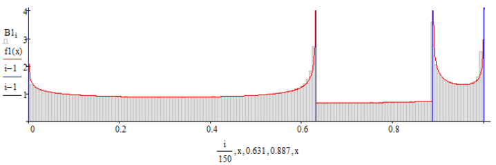
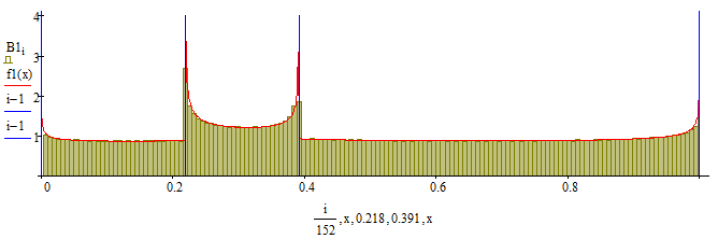
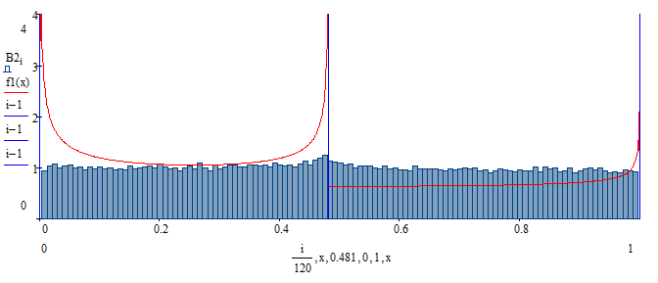
5. Some examples

To illustrate the algorithm and the procedure, we give examples of distributions for some polynomials from the Table 1. Using the definition of $f(x)$ and the well known fact that the first derivative of the function $f(x)$ on a small interval $[a,b]$ could be estimated with the finite difference: $f(b)-f(a)$ divided by $b-a$, we will approximate $f^{\prime}(x)$. The interval $[0,1]$ is divided into $p$ pieces. We compute the fractional part of $P(\theta^{n})$ for $1\leq n\leq N$, and count the number of $n$ so that the fractional part of $P(\theta^{n})$ falls into each of subintervals. The vertical axis indicates the number of such n divided by $N/p$ so that this normalisation results in a relative histogram that is most similar to $f^{\prime}(x)$.

Y. Dupain and J. Lesca [5] conclude that for large degrees t, the sequence $(\{\theta^{n}\})$ is close to being equidistributed, a fact that S. Akiyama and Y. Tanigawa [1] make very explicit in their article. We can notice that the same property is valid for the sequence $(P(\theta^{n}))$ modulo 1 (Fig. 3).

References

- [1] S. Akiyama and Y. Tanigawa, Salem numbers and uniform distribution modulo 1, Publ. Math. Debrecen 64(3–4) (2004), 329–341.
- [2] M.-J. Bertin, A. Decomps-Guilloux, M. Grandet-Hugot, M. Pathiaux-Delefosse, and J.-P. Schreiber, Pisot and Salem numbers, Birkhäuser, Basel, (1992).
- [3] Y. Bugeaud, Distribution modulo one and diophantine approximation, Cambridge Tracts in Mathematics vol. 193 (2012).
- [4] C. Doche, M. Mendès France, J.-J. Ruch, Equidistribution modulo 1 and Salem numbers. Funct. Approx. Comment. Math. 39 (2008), part 2, 261–271.
- [5] Y. Dupain and J. Lesca, Répartition des sous-suites d’une suite donnée. Acta Arith., 23 (1973), 307–314.
- [6] J. C. Mason and D. C. Handscomb, Chebyshev Polynomials, Rhapman & Hall – CRC, Boca Raton London New York Washington D.C., 2003.
- [7] R. Salem, Power series with integral coefficients. Duke Math. J. 12 (1945), 153-172.
- [8] R. Salem, Algebraic Numbers and Fourier Analysis, Heath Math. Monographs, Heath, Boston, 1963.
- [9] Chris Smyth, Seventy years of Salem numbers, Bull. London Math. Soc. (2015) 47 (3): 379-395
- [10] D. Stankov, On spectra of neither Pisot nor Salem algebraic integers, Monatsh. Math. 159 (2010), 115–131.
- [11] D. Stankov, On linear combinations of Chebyshev polynomials, Publ. Inst. Math. 97 (2015), 57–67.