Brownian Dynamics of Confined Rigid Bodies

Abstract

We introduce numerical methods for simulating the diffusive motion of rigid bodies of arbitrary shape immersed in a viscous fluid. We parameterize the orientation of the bodies using normalized quaternions, which are numerically robust, space efficient, and easy to accumulate. We construct a system of overdamped Langevin equations in the quaternion representation that accounts for hydrodynamic effects, preserves the unit-norm constraint on the quaternion, and is time reversible with respect to the Gibbs-Boltzmann distribution at equilibrium. We introduce two schemes for temporal integration of the overdamped Langevin equations of motion, one based on the Fixman midpoint method and the other based on a random finite difference approach, both of which ensure the correct stochastic drift term is captured in a computationally efficient way. We study several examples of rigid colloidal particles diffusing near a no-slip boundary, and demonstrate the importance of the choice of tracking point on the measured translational mean square displacement (MSD). We examine the average short-time as well as the long-time quasi-two-dimensional diffusion coefficient of a rigid particle sedimented near a bottom wall due to gravity. For several particle shapes we find a choice of tracking point that makes the MSD essentially linear with time, allowing us to estimate the long-time diffusion coefficient efficiently using a Monte Carlo method. However, in general such a special choice of tracking point does not exist, and numerical techniques for simulating long trajectories, such as the ones we introduce here, are necessary to study diffusion on long timescales.

I Introduction

The Brownian motion of rigid bodies suspended in a viscous solvent is one of the oldest subjects in nonequilibrium statistical mechanics, and is of crucial importance in a number of applications in chemical engineering and materials science. Examples include the dynamics of passive BoomerangDiffusion ; ColloidalClusters_Granick ; SphereNearWall ; ComplexShapeColloids ; RigidRods_BD ; AsymmetricBoomerangs or active ActiveSuspensions ; Hematites_Science ; FlippingNanorods ; RotationalDiffusion_Lowen particles in suspension, the dynamics of biomolecules in solution HYDROPRO ; HYDROPRO_Globular ; RotationalBD_Torre , the design of novel nano-colloidal materials BiaxialNematic_Boomerang , and others. At the mesoscopic scales of interest, the erratic motion of individual molecules in the solvent drives the diffusive motion of the suspended particles. The number of degrees of freedom necessary to simulate this motion directly using Molecular Dynamics (MD) is large enough to make this approach prohibitively expensive. Instead, the Brownian dynamics approach captures the effect of the solvent through a mobility operator, and thermal fluctuations are modeled using appropriate stochastic forcing terms. In previous work BrownianBlobs , we used a computational fluid solver and immersed boundary techniques to simulate the diffusive motion of spherical particles including hydrodynamic interactions. The fluctuating immersed boundary method developed in BrownianBlobs is suitable for minimally-resolved computations in which only the translational degrees of freedom are kept and hydrodynamics is resolved at a far-field level assuming the particles are spherical. Novel methods are, however, required to model the behavior of particles with nontrivial shapes such as rigidly-fused colloidal clusters ComplexShapeColloids ; ColloidalClusters_Granick or colloidal boomerangs BoomerangDiffusion . In this paper, we show how to include rotational degrees of freedom in the overdamped Langevin equations of motion for rigid bodies suspended in a viscous fluid, develop specialized temporal integrators for these equations, and apply them to a number of model problems.

One of the important goals of our work is to develop an overdamped formulation and associated numerical algorithms that apply when the hydrodynamic mobility (equivalently, resistance) depends strongly on the configuration. Many previous works have focused on the rotational diffusion of a single isolated rigid body in an unbounded domain. However, in practice, rigid particles diffuse either in a suspension, in which case they interact hydrodynamically with other particles, or near a boundary such as a microscope slide or the walls of a slit channel, in which case they interact hydrodynamically with the boundaries. Here we consider a general case of a rigid body performing translational and rotational Brownian motion in a confined system, specifically, we numerically study particles sedimented close to a single no-slip boundary. This is of particular relevance to recent experimental studies of the diffusive motion of colloidal particles that are much denser than water and thus sediment close to the microscope slide (glass plate) ColloidalClusters_Granick ; SphereNearWall ; BoomerangDiffusion .

When writing the equations of motion for a rigid body one must first choose how to represent the orientation of the body. For bodies with a high degree of symmetry one can use simple representations of orientation, for example, for axisymmetric particles (e.g., rigid rods) in three dimensions one can use two polar angles or a unit vector to represent the orientation of the axis of symmetry BD_Rods_Shaqfeh ; RigidRods_BD ; SpheroidNearWall . More complex (biaxial or skewed) particle shapes BoomerangDiffusion ; AsymmetricBoomerangs , or asymmetrically patterned particles of symmetric shapes SphereNearWall , as common in active particle suspensions ActiveSuspensions ; FlippingNanorods , require describing the complete orientation of the rigid bodies. Mathematically, the orientation of a general rigid body in three dimensions is an element of the rotation group $SO(3)$; the group of unitary $3\times 3$ matrices of unit determinant (rotation matrices). This group can be parameterized in a number of ways, the most fundamental one representing elements of this group by an orientated rotation angle, represented as a three-dimensional vector $\boldsymbol{\phi}$, the direction of which gives an axes of rotation relative to a reference configuration, and the magnitude of which gives an angle of rotation around that axes. Prior work on rotational Brownian motion in the overdamped regime has considered the use of Euler angles RotationalDiffusion_Lowen ; Overdamped_EulerAngles , oriented rotation angles Overdamped_AngleRotation , as well as a number of other representations RotationalBD_Doi ; RotationalBD_Torre . Each of these representations has its own set of problems, notably, most of them have singularities or redundancies (which can be avoided in principle with sufficient care), lead to complex analytical expressions involving potentially expensive-to-evaluate trigonometric functions, or require a large amount of storage (e.g., a rotation matrix with $9$ elements). Furthermore, with the exception of RotationalDiffusion_Lowen ; Overdamped_AngleRotation ; Overdamped_EulerAngles , most prior work on rotational diffusion either assumes that the mobility does not depend on configuration RotationalDiffusion_McCammon , focuses on cases where tracking a single axes is sufficient to describe the Brownian motion BD_Rods_Shaqfeh ; RigidRods_BD ; SphereRotation_Wall , or is not careful in handling the stochastic drift terms necessary when the rotational mobility is dependent on the position and orientation of the body.

In molecular dynamics circles LangevinRotation_Inertial ; LangevinRotation_Inertial1 ; Event_Driven_HE , it is well-known that a robust and efficient representation of orientation is provided by unit quaternions, which are unit vectors in four dimensions (i.e., points on the unit 4-sphere). This representation contains one redundant degree of freedom (four instead of the minimal required of three), however, it is free of singularities and thus numerically robust, and, as we will see, leads to a straightforward formulation that is simple to work with both analytically and numerically. In some sense, the quaternion representation is a direct generalization to bi-axial bodies of the standard representation used in Brownian Dynamics of uni-axial particles RigidRods_BD , namely, a unit vector in three dimensions. That common representation is also redundant (only two polar angles are required to describe a direction in three dimensions), however, it offers many advantages over more compressed representations such as polar angles, and is thus the representation of choice. Following the submission of this manuscript, we learned of a very recent work by Ilie et al that also uses quaternions in an overdamped Langevin equation for the motion of a general rigid body in bulk RotationalBD_Quaternions ; earlier work RotationalBD_QuaternionsOld has also used quaternions but without carefully considering the required stochastic drift terms.

We consider the overdamped regime, where the timescale of momentum diffusion in the fluid is much shorter than the timescale of the motion of the rigid bodies themselves. Formally, this regime corresponds to the limit of infinite Schmidt number StokesEinstein . Neglecting inertia, we track only the positions and orientations of the immersed bodies, deriving evolution equations for the quaternion representation. This Langevin system exhibits the correct deterministic dynamics and preserves the Gibbs-Boltzmann distribution in equilibrium, properly restricted to the unit quaternion 4-sphere. Integrating these equations proves challenging primarily due to the presence of the stochastic drift term that arises from the configuration-dependent mobility; this issue is identified theoretically in Appendix C in RotationalBD_Quaternions but that work is focused on unconfined particles for which a key stochastic drift term vanishes (see (C21) in RotationalBD_Quaternions ). The standard approach to handling the stochastic drift term is Fixman’s method, requiring a costly application of the inverse of the mobility which in some cases is not directly computable. As an alternative, we employ a recently-proposed Random Finite Difference (RFD) scheme BrownianBlobs ; MultiscaleIntegrators for approximating the drift; this approach only requires application of the mobility and its “square root” but not the inverse of the mobility.

We perform a number of numerical experiments in which we simulate the Brownian motion of rigid particles sedimented near a wall in the presence of gravity, as inspired by recent experimental studies of the diffusion of asymmetric spheres SphereNearWall , clusters of spheres ColloidalClusters_Granick ; ComplexShapeColloids , and boomerang colloids BoomerangDiffusion ; AsymmetricBoomerangs . In the first example, we study a tetramer formed by rigidly connecting four colloidal spheres placed at the vertices of a tetrahedron, modeling colloidal clusters that have been manufactured in the lab ColloidalClusters_Granick ; ComplexShapeColloids ; ColloidCluster_Holography ; ColloidalCluster_Nano . In the second example, we study the rotational and translational diffusion of an asymmetric colloidal sphere with center of mass displaced from the geometric center, modeling recently-manufactured “colloidal surfers” Hematites_Science in which a dense hematite cube is embedded in a polymeric spherical particle. In the last example we study the quasi two-dimensional diffusive motion of a dense boomerang colloid sedimented near a no-slip boundary, as inspired by recent experiments BoomerangDiffusion ; AsymmetricBoomerangs ; angleBoomerangs . We computationally demonstrate the crucial importance of the choice of tracking point when computing the translational diffusion coefficient. In particular, we show that with a suitable choice of the origin around which torques are expressed, one can obtain an approximate but relatively accurate formula for the effective long-time diffusion coefficient in the directions parallel to the boundary. However, we are unable to reach a precise and definite conclusion about the optimal choice of tracking point even for quasi-two-dimensional diffusion, since for all shapes studied here and in existing experiments the center of hydrodynamic stress and the center of mobility are too close to each other to be distinguished. In the more general case, our results indicate that there is no exact closed-form expression for the long-time quasi-two-dimensional coefficient, and numerical methods for simulating trajectories are necessary in order to study the long-time diffusive dynamics of even a single rigid body in the presence of confinement.

This paper is organized as follows. In Section II, we formulate the equations of motion for rigid bodies with translation and rotation, giving a brief background on the use of quaternions to parameterize orientation. Section III introduces temporal integrators for these equations, including a Fixman scheme, as well as a RFD scheme that approximates the stochastic drift using only applications of the mobility. We perform numerical tests of our schemes in Section IV to verify that we can correctly simulate the dynamics of a rigid body near a no-slip boundary, and study the influence of the choice of tracking point on the MSD. Finally, we give concluding thoughts and discuss future directions in Section V. Technical details are handled in Appendices.

II Langevin equations for rigid bodies

In this section, we formulate Langevin equations for rigid bodies performing rotational and translational diffusion. We begin by formulating an overdamped Langevin equation for rotational diffusion using a unit quaternion representation of rigid-body orientation. For the remainder of this section, we will assume that we know how to compute the configuration dependent hydrodynamic mobilities needed for our equations. These mobility matrices are applied to vectors of forces and torques to compute the resulting linear and angular velocities of the immersed rigid bodies. In future work, we will develop algorithms for computing these objects on the fly using a computational fluid solver as in the Fluctuating Immersed Boundary (FIB) method BrownianBlobs , as we discuss in more detail in Section V.

Our goal is to formulate an equation for the evolution of the orientation of a rigid body. It is important that the resulting system has the correct deterministic term, that it is time reversible with respect to the correct Gibbs-Boltzmann distribution in equilibrium, and that it preserves the constraint that the quaternion has unit norm. Before we accomplish this goal, we briefly review some required facts about quaternions.

II.1 Quaternions

Describing the orientation of a rigid body in three dimensions can be done in many ways. Rotation matrices are perhaps the most straightforward approach to accomplish this task, but they require the use of 9 floating point numbers to parameterize a 3 dimensional space. Additionally, accumulation of numerical errors over many time steps can cause rotation matrices to lose their orthonormal properties. Euler angles suffer from gimbal lock, where at certain orientations, two Euler angles describe rotation about the same axis, and a degree of freedom is lost. Oriented angles are inconvenient to accumulate (in particular one cannot simply add oriented angles to represent successive rotations) and require the evaluation of trigonometric functions. In this work, we choose to use normalized quaternions, which require 4 floating point numbers to store, are easy to normalize, can be accumulated in a convenient manner, and avoid the need for (potentially expensive to evaluate) trigonometric functions.

A normalized quaternion can be used to represent a finite rotation relative to a given initial reference frame, and is specified by $\boldsymbol{\theta}=\{s,\boldsymbol{p}\}\in\mathbb{R}^{4},$ a combination of a scalar $s$ and a vector $\boldsymbol{p}\in\mathbb{R}^{3}$ that satisfy the unit-norm constraint

$$\left\|\boldsymbol{\theta}\right\|^{2}=s^{2}+\boldsymbol{p}\cdot\boldsymbol{p}=1.$$ (1)

Quaternions can be combined via the operation of quaternion multiplication, whereby $\boldsymbol{\theta}_{3}=\boldsymbol{\theta}_{1}\boldsymbol{\theta}_{2}$ is defined via

$$\left[\begin{array}[]{c}s_{3}\\ \boldsymbol{p}_{3}\end{array}\right]= \left[\begin{array}[]{c}s_{1}s_{2}-\boldsymbol{p}_{1}\cdot\boldsymbol{p}_{2}\\ s_{1}\boldsymbol{p}_{2}+s_{2}\boldsymbol{p}_{1}+\boldsymbol{p}_{1}\times\boldsymbol{p}_{2}\end{array}\right],$$ (6)

with $\boldsymbol{\theta}_{i}=\{s_{i},\,\boldsymbol{p}_{i}\},\,i=1,2,3$. With this operation, normalized quaternions form a group with identity $\{1,\,\boldsymbol{0}\}$; the inverse of a quaternion $\boldsymbol{\theta}=\{s,\boldsymbol{p}\}$ is given by $\boldsymbol{\theta}^{-1}=\{s,-\boldsymbol{p}\}$.

In this work, we will use normalized quaternions to represent the orientation of a body in three space dimensions. Any finite rotation can be defined by its oriented angle, a vector $\boldsymbol{\phi}$, indicating a turn of $\phi=\left\|\boldsymbol{\phi}\right\|$ radians counterclockwise (i.e., using the right-hand convention) around an axis $\hat{\boldsymbol{\phi}}=\boldsymbol{\phi}/\phi$. This rotation can be associated with the quaternion

$$\boldsymbol{\theta}_{\boldsymbol{\phi}}=\{\cos(\phi/2),\,\sin(\phi/2)\hat{\boldsymbol{\phi}}\},$$ (7)

i.e., $\boldsymbol{p}$ gives the axis of the rotation and the magnitude of $\boldsymbol{p}$ gives the angle of rotation; the inclusion of $s$ and the normalization constraint is thus not strictly necessary IsotropicRotationalDiffusion but is useful numerically. Note that $\boldsymbol{\theta}$ and $-\boldsymbol{\theta}$ correspond to the same physical rotation/orientation .

Performing a rotation on any three dimensional vector $\boldsymbol{r}$ in the reference frame gives a rotated vector $\boldsymbol{r}^{\prime}=\boldsymbol{R}(\boldsymbol{\theta})\boldsymbol{r}$, where the rotation matrix is

$$\boldsymbol{R}(\boldsymbol{\theta})=2\left[\boldsymbol{p}\boldsymbol{p}^{T}+s\boldsymbol{P}+\left(s^{2}-\frac{1}{2}\right)\boldsymbol{I}\right].$$

Here $\boldsymbol{P}$ is a cross-product $3\times 3$ matrix such that $\boldsymbol{P}\boldsymbol{r}=\boldsymbol{p}\times\boldsymbol{r}$ for any $\boldsymbol{r}$, i.e., $P_{ij}=\epsilon_{ikj}p_{k}$, where $\epsilon$ is the Levi-Civita symbol. Given two normalized quaternions $\boldsymbol{\theta}_{1}$ and $\boldsymbol{\theta}_{2}$, their rotation matrices satisfy the condition

$$\boldsymbol{R}(\boldsymbol{\theta}_{1})\boldsymbol{R}(\boldsymbol{\theta}_{2})=\boldsymbol{R}(\boldsymbol{\theta}_{1}\boldsymbol{\theta}_{2}),$$ (8)

that is, successive rotations can be accumulated by multiplying their associated quaternions. More precisely, if a rotation given by oriented angle $\boldsymbol{\phi}$ followed by a rotation $\boldsymbol{\psi}$ yields a total rotation $\boldsymbol{\zeta}$, then it holds that $\boldsymbol{\theta}_{\boldsymbol{\zeta}}=\boldsymbol{\theta}_{\boldsymbol{\psi}}\boldsymbol{\theta}_{\boldsymbol{\phi}}$.

Given an angular velocity $\boldsymbol{\omega}$, we can write the corresponding time derivative of orientation as

$$\dot{\boldsymbol{\theta}}=\boldsymbol{\Psi}\boldsymbol{\omega},$$ (9)

where $\boldsymbol{\Psi}\left(\boldsymbol{\theta}\right)$ is the $4\times 3$ matrix

$$\boldsymbol{\Psi=}\frac{1}{2}\left[\begin{array}[]{c}-\boldsymbol{p}^{T}\\ s\boldsymbol{I}-\boldsymbol{P}\end{array}\right].$$ (10)

The matrix $\boldsymbol{\Psi}$ has many properties that will be useful when we formulate equations of motion for bodies with orientation. First, it satisfies the property

$$\boldsymbol{\Psi}^{T}\boldsymbol{\theta}=\frac{1}{2}\left(-s\boldsymbol{p}+s\boldsymbol{p}\right)=\boldsymbol{0},$$ (11)

which together with the relation $\dot{\boldsymbol{\theta}}=\boldsymbol{\Psi}\boldsymbol{\omega}$, indicates that the deterministic evolution (9) remains on the constraint (1). This property is used in Section II to show that the Langevin equations presented in this work also preserve the constraint. Another useful relationship is the fact that

$$\partial_{\boldsymbol{\theta}}\cdot\boldsymbol{\Psi}^{T}=0\quad\mbox{i.e.}\quad\partial_{l}\left(\Psi_{lk}\right)=0,$$ (12)

which is clear because the $j$-th row of $\boldsymbol{\Psi}$ has no entries that depend on the $j$-th component of $\boldsymbol{\theta}$. Here and in the remainder of this paper we use Einstein’s repeated index summation convention, and denote $\partial_{j}\equiv\partial/\partial\theta_{j}$.

Describing the orientation of a body at several times $t^{n}$ requires choosing a single initial reference orientation associated with $\boldsymbol{\theta}^{0}=\left\{1,\boldsymbol{0}\right\}$, and recording the quaternion $\boldsymbol{\theta}^{n}$ that describes the rotation from the reference orientation to the orientation at instant $t^{n}$. Furthermore, if the body undergoes a rotation with constant angular velocity $\boldsymbol{\omega}$ from time $t^{n}$ to time $t^{n+1}=t^{n}+\Delta t,$ we have that $\boldsymbol{\theta}^{n+1}=\boldsymbol{\theta}_{\boldsymbol{\omega}\Delta t}\boldsymbol{\theta}^{n}$. This leads to a natural recipe for tracking orientation using the Rotate procedure

$$\boldsymbol{\theta}^{n+1}=\mbox{Rotate(}\boldsymbol{\theta}^{n},\,\boldsymbol{\omega}\Delta t)=\boldsymbol{\theta}_{\boldsymbol{\omega}\Delta t}\boldsymbol{\theta}^{n}.$$ (13)

In constructing numerical schemes in Section III, it will be necessary to consider the second order expansion of this rotate procedure

$$\mbox{Rotate(}\boldsymbol{\theta},\,\boldsymbol{\omega}\Delta t)= \boldsymbol{\theta}+\boldsymbol{\Psi}\boldsymbol{\omega}\Delta t-\frac{\left(\boldsymbol{\omega}\cdot\boldsymbol{\omega}\right)\Delta t^{2}}{8}\boldsymbol{\theta}+O\left(\Delta t^{3}\right),$$ (14)

as shown in Appendix (A.1).

II.2 Rotational Brownian Motion

For simplicity, we first consider a single rigid body that is free to rotate but with a reference point $\boldsymbol{q}$, around which torques are measured, that is fixed in space. We let the orientation of this body (relative to some fixed reference frame) be denoted by the quaternion $\boldsymbol{\theta}\left(t\right)$, and we suppose that the body is subjected to a torque $\boldsymbol{\tau}$ generated by a given conservative potential $U(\boldsymbol{\theta})$. It can be shown (see Appendix A.2) the the torque generated by the potential is

$$\boldsymbol{\tau}= -\boldsymbol{\Psi}^{T}\partial_{\boldsymbol{\theta}}U$$ (15)

In practice, it is not necessary to formulate $U(\boldsymbol{\theta})$ and calculate $-\boldsymbol{\Psi}^{T}\partial U/\partial\boldsymbol{\theta}$ to obtain the torque. Often is is much more convenient to calculate torque directly based on the geometries of the rigid bodies and the forces applied to them. We will see that (15) will be a convenient relation for formulating the constrained equations of motion. The schemes that we develop will be able to simulate the motion of rigid bodies without direct knowledge of $U(\boldsymbol{\theta})$; they simply update the positions and orientations of the bodies based on the total forces and torques applied to each body.

II.2.1 Overdamped Langevin Equation

We introduce the $3\times 3$ symmetric positive semidefinite (SPD) rotational mobility matrix $\boldsymbol{M}_{\boldsymbol{\omega}\boldsymbol{\tau}}\left(\boldsymbol{\theta}\right)$, which acts on torque to produce the resulting angular velocity, $\boldsymbol{\omega}=\boldsymbol{M}_{\boldsymbol{\omega}\boldsymbol{\tau}}\boldsymbol{\tau}$. Note that the mobility contains all the effects of hydrodynamics, including the shape of the body, the hydrodynamic interactions with other bodies or boundaries, far-field boundary conditions, etc. In this section we will assume this matrix is known, and discuss ways to obtain it explicitly in Section IV. Using (9) and (15), we can write down a deterministic equation of motion for the rigid body,

$$\frac{d\boldsymbol{\theta}}{dt}= \boldsymbol{\Psi}\boldsymbol{M}_{\boldsymbol{\omega}\boldsymbol{\tau}}\boldsymbol{\tau}=-\left(\boldsymbol{\Psi}\boldsymbol{M}_{\boldsymbol{\omega}\boldsymbol{\tau}}\boldsymbol{\Psi}^{T}\right)\partial_{\boldsymbol{\theta}}U=-\widetilde{\boldsymbol{M}}\,\partial_{\boldsymbol{\theta}}U,$$

where we have defined the $4\times 4$ mobility matrix $\widetilde{\boldsymbol{M}}=\boldsymbol{\Psi}\boldsymbol{M}_{\boldsymbol{\omega\tau}}\boldsymbol{\Psi}^{T}$.

It is now straight forward to formulate an Ito Langevin equation for the rotational diffusion of the body,

$$\frac{d\boldsymbol{\theta}}{dt}= -\widetilde{\boldsymbol{M}}\partial_{\boldsymbol{\theta}}U+\sqrt{2k_{B}T}\;\widetilde{\boldsymbol{M}}^{\frac{1}{2}}\boldsymbol{\mathcal{W}}+\left(k_{B}T\right)\partial_{\boldsymbol{\theta}}\cdot\widetilde{\boldsymbol{M}},$$ (16)

where $\boldsymbol{\mathcal{W}}(t)$ is a collection of independent white noise processes. Here $\widetilde{\boldsymbol{M}}^{\frac{1}{2}}=\boldsymbol{\Psi}\boldsymbol{M}_{\boldsymbol{\omega}\boldsymbol{\tau}}^{\frac{1}{2}}$, with the “square root” of the mobility $\boldsymbol{M}_{\boldsymbol{\omega}\boldsymbol{\tau}}^{\frac{1}{2}}$ obeying the fluctuation-dissipation relation $\boldsymbol{M}_{\boldsymbol{\omega}\boldsymbol{\tau}}^{\frac{1}{2}}\left(\boldsymbol{M}_{\boldsymbol{\omega}\boldsymbol{\tau}}^{\frac{1}{2}}\right)^{T}=\boldsymbol{M}_{\boldsymbol{\omega}\boldsymbol{\tau}}$, for example, it could be the Cholesky factor of $\boldsymbol{M}_{\boldsymbol{\omega}\boldsymbol{\tau}}$. Note that in (16) the covariance for the noise satisfies the fluctuation dissipation balance condition $\widetilde{\boldsymbol{M}}^{\frac{1}{2}}\left(\widetilde{\boldsymbol{M}}^{\frac{1}{2}}\right)^{T}=\widetilde{\boldsymbol{M}}.$ The $i$-th component of the stochastic drift term $\partial_{\boldsymbol{\theta}}\cdot\widetilde{\boldsymbol{M}}$ may be written in indicial notation as $\partial_{j}\widetilde{M}_{ji}(\boldsymbol{\theta})$.

Using Ito’s formula, we can show that the overdamped dynamics (16) strictly preserves the constraint that $\boldsymbol{\theta}$ have unit norm,

$$\frac{d}{dt}\left(\boldsymbol{\theta}^{T}\boldsymbol{\theta}\right)=\boldsymbol{\theta}^{T}\frac{d\boldsymbol{\theta}}{dt}+\left(k_{B}T\right)\boldsymbol{I}:\widetilde{\boldsymbol{M}}=\left(k_{B}T\right)\left(\boldsymbol{\theta}^{T}\left(\partial_{\boldsymbol{\theta}}\cdot\widetilde{\boldsymbol{M}}\right)+\boldsymbol{I}:\widetilde{\boldsymbol{M}}\right)=\left(k_{B}T\right)\partial_{\boldsymbol{\theta}}\cdot\left(\boldsymbol{\theta}^{T}\widetilde{\boldsymbol{M}}\right)=0,$$

where we used (11) and its consequence $\boldsymbol{\theta}^{T}\widetilde{\boldsymbol{M}}=0$. Note that the stochastic drift term in (16) can be rewritten as (see Appendix B),

$$\partial_{\theta}\cdot\widetilde{\boldsymbol{M}}=\partial_{\theta}\cdot\left(\boldsymbol{\Psi}\boldsymbol{M}_{\boldsymbol{\omega}\boldsymbol{\tau}}\boldsymbol{\Psi}^{T}\right)=\boldsymbol{\Psi}\left(\partial_{\boldsymbol{\theta}}\boldsymbol{M}_{\boldsymbol{\omega}\boldsymbol{\tau}}\right):\boldsymbol{\Psi}^{T}-\frac{1}{4}\text{Tr}\left(\boldsymbol{M}_{\boldsymbol{\omega}\boldsymbol{\tau}}\right)\boldsymbol{\theta},$$ (17)

where Tr denotes trace, and colon denotes double contraction; in index notation $\left(\boldsymbol{\Psi}\left(\partial_{\boldsymbol{\theta}}\boldsymbol{M}_{\boldsymbol{\omega}\boldsymbol{\tau}}\right):\boldsymbol{\Psi}^{T}\right)_{i}=\Psi_{ij}\partial_{l}\left(M_{\boldsymbol{\omega}\boldsymbol{\tau}}\right)_{jk}\Psi_{lk}$ and $\left\{\text{Tr}\left(\boldsymbol{M}_{\boldsymbol{\omega}\boldsymbol{\tau}}\right)\boldsymbol{\theta}\right\}_{i}=\left(M_{\boldsymbol{\omega}\boldsymbol{\tau}}\right)_{jj}\theta_{i}$ . We will see that this way of writing the drift is convenient when we consider numerical methods for integrating (16) in Section III. Note that the stochastic drift term proportional to $\text{Tr}\left(\boldsymbol{M}_{\boldsymbol{\omega}\boldsymbol{\tau}}\right)\boldsymbol{\theta}/4$ can be seen in Eq. (36) in RotationalBD_Quaternions to be related to enforcing the normalization constraint, and it will turn out we do not need to include it explicitly just as in RotationalBD_Quaternions .

In the special case of a free particle with unit mobility, $\boldsymbol{M}_{\boldsymbol{\omega}\boldsymbol{\tau}}=\boldsymbol{I}$, (16) degenerates to the Stratonovich equation (see (38)),

$$\dot{\boldsymbol{\theta}}=\left(2k_{B}T\right)^{\frac{1}{2}}\boldsymbol{\Psi}\circ\boldsymbol{\mathcal{W}}.$$ (18)

Recall that the infinitesimal change in orientation is given by the infinitesimal rotation $d\boldsymbol{\phi}$ in the axes-angle representation, where the direction of the vector $d\boldsymbol{\phi}$ is the axes around which the body is rotated by an angle $d\phi$. Also recall that the corresponding change in the quaternion is

$$d\boldsymbol{\theta}=\boldsymbol{\Psi}\left(\boldsymbol{\theta}\right)d\boldsymbol{\phi},$$

at least deterministically. Since the standard rules of calculus apply in the Stratonovich interpretation, (18) is equivalent to

$$d\boldsymbol{\varphi}=\left(2k_{B}T\right)^{\frac{1}{2}}d\boldsymbol{\mathcal{B}}$$ (19)

where $\boldsymbol{\mathcal{B}}\left(t\right)$ is Brownian motion, formally $\boldsymbol{\mathcal{W}}\equiv d\boldsymbol{\mathcal{B}}/dt$. This is a natural definition of isotropic rotational diffusion IsotropicRotationalDiffusion .

We can verify that (16) has the correct noise covariance when $\boldsymbol{M}_{\boldsymbol{\omega}\boldsymbol{\tau}}$ is not a multiple of the identity by considering the rotational mean square displacement at short times. Let us consider a set of orthonormal vectors $\boldsymbol{u}_{i}(t)$ which are attached to the rigid body, and define a rotational displacement following Kraft et al. ComplexShapeColloids ,

$$\Delta\hat{\boldsymbol{u}}\left(\Delta t\right)\equiv\frac{1}{2}\sum_{i=1}^{3}\boldsymbol{u}_{i}(0)\times\boldsymbol{u}_{i}\left(\Delta t\right).$$ (20)

A straightforward calculation relates this rotational displacement to the total angle of rotation $\boldsymbol{\phi}_{\Delta t}$ relative to the the initial configuration,

$$\Delta\hat{\boldsymbol{u}}\left(\Delta t\right)=\sin\left(\phi_{\Delta t}\right)\hat{\boldsymbol{\phi}}_{\Delta t}=\boldsymbol{\phi}_{\Delta t}+O(\Delta t^{\frac{3}{2}}),$$ (21)

which shows that the magnitude of the rotational displacement is insensitive to the choice of the initial triad $\boldsymbol{u}_{i}(0)$. If the covariance of the noise in (16) is correct, it should hold that (c.f. Eqs. (1,2) in Ref. ComplexShapeColloids )

$$\frac{1}{2k_{B}T}\,\lim_{\Delta t\to 0}\frac{\langle\left(\Delta\hat{\boldsymbol{u}}\left(\Delta t\right)\right)\left(\Delta\hat{\boldsymbol{u}}\left(\Delta t\right)\right)^{T}\rangle}{\Delta t}=\frac{1}{2k_{B}T}\,\lim_{\Delta t\to 0}\left(\frac{\boldsymbol{\phi}_{\Delta t}\boldsymbol{\phi}_{\Delta t}^{T}}{\Delta t}\right)= \boldsymbol{M}_{\boldsymbol{\omega}\boldsymbol{\tau}},$$ (22)

which follows directly from (16). This shows that our equation has the same physical noise covariance as the overdamped equation in Ref. ComplexShapeColloids , only written in a different representation. In our numerical tests, we will use $\langle\left(\Delta\hat{\boldsymbol{u}}\left(\tau\right)\right)\left(\Delta\hat{\boldsymbol{u}}\left(\tau\right)\right)^{T}\rangle$ as a convenient definition of a rotational mean square displacement (RMSD) at time $\tau$; note that this RMSD is necessarily bounded and thus must reach a plateau at long times.

II.2.2 Smoluchowski Equation

A key property of the overdamped Langevin equation (16) is that it is time reversible with respect to the Gibbs-Boltzmann equilibrium distribution

$$P_{\text{eq}}\left(\boldsymbol{\theta}\right)=Z^{-1}\exp\left(-U\left(\boldsymbol{\theta}\right)/k_{B}T\right)\delta\left(\boldsymbol{\theta}^{T}\boldsymbol{\theta}-1\right),$$ (23)

with $Z$ a normalization constant. The overdamped equation (16) has the familiar structure of a generic Langevin equation (see Section I.A in Ref. MultiscaleIntegrators ); however, a crucial difference is that (16) is an SDE on a manifold, namely, the unit 4-sphere, rather than an SDE in Eucledian space. A discussion of overdamped Langevin equations constrained on a manifold can be found in Ref. ConstrainedStochasticDiffusion . As explained there, for general curved manifolds one has to carefully construct the stochastic drift terms in order to ensure consistency with the desired equilibrium distribution. Note that the original (true or physical) dynamics is unconstrained, and could, in principle, be described using a non-redundant parameterization of the rotation group such as Euler angles RotationalDiffusion_Lowen ; the unit norm constraint implicit in (16) arises because it is mathematically simpler to embed the unit 4-sphere in a four dimensional Euclidean space than to parameterize it directly. The geometric matrix $\boldsymbol{\Psi}\left(\boldsymbol{\theta}\right)$ plays the role of the projection operator in Ref. ConstrainedStochasticDiffusion , but unlike a projection operator, $\boldsymbol{\Psi}$ is not square and projects from the original (physical) three-dimensional space of angular velocity to the tangent space of the unit 4-sphere.

To see that (23) is indeed the equilibrium distribution let us consider the case of a freely-rotating particle, $U\left(\boldsymbol{\theta}\right)=0$, which should correspond to uniform probability of all orientations. The uniform distribution over the space of orientations of a rigid body in three dimensions is the so-called Haar measure over the group $SO(3)$, and has been the subject of mathematical study rummler2002distribution ; miles1965random . It is known that in the quaternion representation this Haar measure corresponds to a constant probability density over the surface of the unit 4-sphere, i.e., the Hausdorff measure on the unit 4-sphere rummler2002distribution ; prentice1978invariant ; IsotropicRotationalDiffusion ; generating random uniformly-distributed orientations amounts to simply generating a point uniformly sampled on the unit 4-sphere . This uniform distribution over the unit quaternion sphere is captured in (23) by the term $\delta\left(\boldsymbol{\theta}^{T}\boldsymbol{\theta}-1\right)$, and the additional prefactor $\exp\left(-U\left(\boldsymbol{\theta}\right)/k_{B}T\right)$ captures the standard Gibbs-Boltzmann weighting of the configurations based on their potential energy.

Note that more generally, for a manifold $\Sigma$ defined by the scalar constraint $g(\boldsymbol{\theta})=0,$ the Hausdorff measure $d\sigma_{\Sigma}$ on the the surface contains a metric factor relative to the Lebesque measure $d\boldsymbol{\theta}$ in unconstrained coordinates, as given by the co-area formula ConstrainedStochasticDiffusion ,

$$d\sigma_{\Sigma}(\boldsymbol{\theta})=\delta\left(g(\boldsymbol{\theta})\right)\left\|\boldsymbol{\nabla}g(\boldsymbol{\theta)}\right\|_{2}\,d\boldsymbol{\theta}.$$

In our case, however, $g(\boldsymbol{\theta})=\boldsymbol{\theta}^{T}\boldsymbol{\theta}-1$ and $\left\|\boldsymbol{\nabla}g(\boldsymbol{\theta)}\right\|_{2}=\left\|\boldsymbol{\theta}\right\|_{2}=1$ is constant over the surface of the unit 4-sphere, and the metric factor can be absorbed into the normalization factor $Z$. The fact that no metric factors appear in the quaternion representation simplifies the equations; in other representations such as Euler angles or rotation angles the Gibbs-Boltzmann distribution is not uniform even in the absence of external potentials, and therefore “metric forces” need to be included in the stochastic drift terms to ensure the correct equilibrium distribution Overdamped_AngleRotation ; Overdamped_EulerAngles . This subtle point has been missed in a number of prior works even though the concept of metric forces is well understood for rather general constrained Langevin equations ConstrainedBD .

To demonstrate that (23) is the equilibrium distribution (invariant measure) for (16), we examine the Fokker-Planck equation (FPE) for the probability density $P\left(\boldsymbol{\theta},t\right)$,

$$\partial_{t}P =\partial_{i}\left\{\widetilde{M}_{ij}\left[\left(\partial_{j}U\right)P+\left(k_{B}T\right)\partial_{j}P\right]\right\}.$$ (24)

When $P$ is the Gibbs-Boltzmann distribution (23), we formally obtain

$$\left[\left(\partial_{j}U\right)P_{\mbox{eq}}+\left(k_{B}T\right)\partial_{j}P_{\mbox{eq}}\right]\sim \exp\left(-U\left(\boldsymbol{\theta}\right)/k_{B}T\right)\delta^{\prime}\left(\boldsymbol{\theta}^{T}\boldsymbol{\theta}-1\right)\theta_{j}.$$

We can then use the fact that $\boldsymbol{\Psi}^{T}\boldsymbol{\theta}=0$ to see that at thermodynamic equilibrium the thermodynamic driving force inside the square brackets in (24) vanishes, which implies that the Gibbs-Boltzmann distribution is an equilibrium distribution; using standard tools combined with reasonable assumptions on $U(\boldsymbol{\theta})$, it can also be shown that (23) is the unique invariant measure ConstrainedStochasticDiffusion . Note that the calculation above is formal, but one can make a more precise argument by considering the backward Kolmogorov equation applied to $\mathbb{E}\left[f\right]$ for an arbitrary well behaved function $f$ and expressing expectation values as integrals over the unit 4-sphere, similar to the approach taken in ConstrainedStochasticDiffusion . A similar calculation can be used to show that the generator of the Markov diffusion process (16) is self-adjoint with respect to a dot product weighted by the invariant measure (23), which proves that the overdamped dynamics is time reversible with respect to (23).

We can compare the Eq. (24) with the FPE derived for rigid rods in Ref. RigidRods_BD . A rigid rod can be parameterized with a unit 3-vector $\boldsymbol{\psi}$ indicating the orientation of the rod. If we expand (24) and use the property (12), we can rewrite the FPE in the form

$$\partial_{t}P= \partial_{i}\left\{\Psi_{ik}\left(M_{\boldsymbol{\omega}\boldsymbol{\tau}}\right)_{kl}\Psi_{jl}\left[\left(\partial_{j}U\right)P+\left(k_{B}T\right)\partial_{j}P\right]\right\}$$

$$= \Psi_{ik}\partial_{i}\left\{\left(M_{\boldsymbol{\omega}\boldsymbol{\tau}}\right)_{kl}\left(\Psi_{jl}\left(\partial_{j}U\right)P+\left(k_{B}T\right)\Psi_{jl}\partial_{j}P\right)\right\}.$$

This FPE has exactly the same form as the rotational part of Eq. (4.149) in RigidRods_BD , with the crucial difference that for rods $\boldsymbol{\Psi}$ is the cross product matrix corresponding to the direction $\boldsymbol{\psi}$. We see that (24) is a natural generalization of the standard Smoluckowski equation for uniaxial bodies to biaxial bodies.

II.3 Rotation-Translation Coupling

In order to describe Brownian motion of freely suspended particles, it is necessary to also include translation in our model of rigid body motion. We first consider tracking both the location and orientation of a single rigid body. To do this, we introduce a variable $\boldsymbol{q}\left(t\right)$ for the Cartesian coordinates of a chosen tracking point fixed in the body frame. We assume that we are given hydrodynamic information in the form of a known grand mobility matrix $\boldsymbol{N}\left(\boldsymbol{q},\boldsymbol{\theta}\right)$, which is the linear mapping from given force $\boldsymbol{F}$ and torque $\boldsymbol{\tau}$ (about $\boldsymbol{q}$) to the resulting velocity $\boldsymbol{u}\equiv\dot{\boldsymbol{q}}$ and angular velocity $\boldsymbol{\omega}$,

$$\left[\begin{array}[]{c}\boldsymbol{u}\\ \boldsymbol{\omega}\end{array}\right]=\boldsymbol{N}\left[\begin{array}[]{c}\boldsymbol{F}\\ \boldsymbol{\tau}\end{array}\right]= \left[\begin{array}[]{cc}\boldsymbol{M}_{\boldsymbol{u}\boldsymbol{F}}&\boldsymbol{M}_{\boldsymbol{u}\boldsymbol{\tau}}\\ \boldsymbol{M}_{\boldsymbol{\omega}\boldsymbol{F}}&\boldsymbol{M}_{\boldsymbol{\omega}\boldsymbol{\tau}}\end{array}\right]\left[\begin{array}[]{c}\boldsymbol{F}\\ \boldsymbol{\tau}\end{array}\right],$$ (33)

where $\boldsymbol{M}_{\boldsymbol{u}\boldsymbol{\tau}}=\boldsymbol{M}_{\boldsymbol{\omega}\boldsymbol{F}}^{T}$ is the translation-rotation coupling tensor, and $\boldsymbol{M}_{\boldsymbol{u}\boldsymbol{F}}$ is the translation-translation mobility familiar from Brownian Dynamics of spherical particles.

Let us suppose that the torque and force are generated from a conservative potential $U(\boldsymbol{q},\boldsymbol{\theta})$. Then using the fact that $\dot{\boldsymbol{q}}=\boldsymbol{u}$, along with (9) and (15) we can write the overdamped Langevin equation including translation as the Ito SDE,

$$\boldsymbol{\upsilon}=\frac{d\boldsymbol{x}}{dt}= -\widetilde{\boldsymbol{N}}\partial_{\boldsymbol{x}}U+\sqrt{2k_{B}T}\,\widetilde{\boldsymbol{N}}^{\frac{1}{2}}\boldsymbol{\mathcal{W}}+\left(k_{B}T\right)\partial_{\boldsymbol{x}}\cdot\widetilde{\boldsymbol{N}}$$ (34)

$$= -\left(\boldsymbol{\Xi}\boldsymbol{N}\boldsymbol{\Xi}^{T}\right)\partial_{\boldsymbol{x}}U+\sqrt{2k_{B}T}\,\boldsymbol{\Xi}\boldsymbol{N}^{\frac{1}{2}}\boldsymbol{\mathcal{W}}+\left(k_{B}T\right)\partial_{\boldsymbol{x}}\cdot\left(\boldsymbol{\Xi}\boldsymbol{N}\boldsymbol{\Xi}^{T}\right),$$

where $\boldsymbol{x}=\left(\boldsymbol{q},\boldsymbol{\theta}\right)^{T}$ and $\boldsymbol{\upsilon}=\left(\boldsymbol{u},\dot{\boldsymbol{\theta}}\right)^{T}$ are composite vectors of the translational and rotational variables (and their velocities), and we have introduced the block matrix

$$\boldsymbol{\Xi}=\left[\begin{array}[]{cc}\boldsymbol{I}&\boldsymbol{0}\\ \boldsymbol{0}&\boldsymbol{\Psi}\end{array}\right].$$ (35)

The “square root” of the mobility $\boldsymbol{N}^{\frac{1}{2}}$ satisfies the fluctuation-dissipation relation $\boldsymbol{N}^{\frac{1}{2}}\left(\boldsymbol{N}^{\frac{1}{2}}\right)^{T}=\boldsymbol{N}$. A similar computation to that mentioned in Section II.2 shows that (34) is time reversible with respect to the Gibbs-Boltzmann distribution ConstrainedStochasticDiffusion ,

$$P_{\mbox{eq}}(\boldsymbol{q},\boldsymbol{\theta})= Z^{-1}\exp\left(-U\left(\boldsymbol{q},\boldsymbol{\theta}\right)/k_{B}T\right)\delta\left(\boldsymbol{\theta}^{T}\boldsymbol{\theta}-1\right).$$ (36)

III Temporal Integrators

In this section we introduce temporal integrators for the overdamped equations of motion of rigid bodies immersed in fluid, as formulated in Section II. We update the quaternion representation of orientation using the Rotate procedure (13) introduced in Section II.1, preserving the unit-norm constraint to numerical precision. The stochastic drift term in (34) is approximated in two ways, using a Fixman midpoint scheme and a Random Finite Difference (RFD) scheme, see Section I.B in Ref. MultiscaleIntegrators for a comparison of the two approaches in the context of unconstrained overdamped Langevin equations.

III.1 Euler-Maruyama scheme

For illustration purposes, we begin by considering a naive Euler-Maruyama (EM) scheme applied to an incorrect variant of (16), in which we do not carefully handle the stochastic drift term $\left(k_{B}T\right)\partial_{\boldsymbol{\theta}}\cdot\widetilde{\boldsymbol{M}}$. In the EM scheme, we advance the configuration from time level $n$ to time level $n+1$ with the time step

$$\boldsymbol{\omega}^{n}= -\boldsymbol{M}_{\boldsymbol{\omega}\boldsymbol{\tau}}^{n}\boldsymbol{\tau}^{n}+\left(\frac{2k_{B}T}{\Delta t}\boldsymbol{M}_{\boldsymbol{\omega}\boldsymbol{\tau}}^{n}\right)^{\frac{1}{2}}\boldsymbol{W}^{n}$$ (37)

$$\boldsymbol{\theta}^{n+1}= \text{Rotate}\left(\boldsymbol{\theta}^{n},\,\boldsymbol{\omega}^{n}\Delta t\right),$$

where a superscript denotes the point in time at which a particular quantity is evaluated, e.g. $\boldsymbol{\theta}^{n}\approx\boldsymbol{\theta}(n\Delta t)$ and $\boldsymbol{M}_{\boldsymbol{\omega}\boldsymbol{\tau}}^{n}=\boldsymbol{M}_{\boldsymbol{\omega}\boldsymbol{\tau}}\left(\boldsymbol{\theta}^{n}\right)$, and the Rotate procedure is defined by (13). Here $\boldsymbol{W}^{n}$ is a collection of i.i.d. standard (i.e., mean zero and unit variance) Gaussian variates generated using a pseudo-random number generator. Here and henceforth, we have used (15) to express the updates directly in terms of torque $\boldsymbol{\tau}(\boldsymbol{\theta})$. While the scheme (37) is not actually consistent with (16), it makes a natural starting point when discussing temporal integrators for (16).

Note that because we use the Rotate procedure (13), this update actually moves along the unit norm constraint of normalized quaternions, as opposed to stepping off of the constraint and then projecting back onto it ConstrainedStochasticDiffusion . This is a natural way to update orientation multiplicatively while still being consistent with the additive Langevin equations formulated in Section II. In the alternative approach followed in RotationalBD_Quaternions one has to solve a quadratic equation (c.f. (15) in RotationalBD_Quaternions ) for a Lagrange multiplier to enforce the normalization constraint; while this avoids the use of trigonometric functions, it is difficult to make such methods second-order accurate. We can expand the Rotate procedure using the Taylor series (14) and truncate the result at first order in $\Delta t$, to obtain an expression for the leading order change in $\boldsymbol{\theta}$,

$$\frac{\boldsymbol{\theta}^{n+1}-\boldsymbol{\theta}^{n}}{\Delta t}\approx \boldsymbol{\Psi}^{n}\boldsymbol{\omega}^{n}-\Delta t\frac{\left(\boldsymbol{\omega}^{n}\cdot\boldsymbol{\omega}^{n}\right)}{8}\boldsymbol{\theta}^{n}.$$

$$= \boldsymbol{\Psi}^{n}\left(-\boldsymbol{M}_{\boldsymbol{\omega}\boldsymbol{\tau}}^{n}\boldsymbol{\tau}^{n}+\left(2k_{B}T\,\boldsymbol{M}_{\boldsymbol{\omega}\boldsymbol{\tau}}^{n}\right)^{\frac{1}{2}}\boldsymbol{W}^{n}\right)$$

$$-\left(k_{B}T\right)\frac{\left(\boldsymbol{W}^{n}\right)^{T}\boldsymbol{M}_{\boldsymbol{\omega}\boldsymbol{\tau}}^{n}\boldsymbol{W}^{n}}{4}\boldsymbol{\theta}^{n}+O\left(\Delta t\right).$$

Note that the last term is equal in expectation to $-k_{B}T\left(\text{Tr}\left(\boldsymbol{M}_{\boldsymbol{\omega}\boldsymbol{\tau}}^{n}\right)/4\right)\boldsymbol{\theta}^{n}$, which gives us the second term in the stochastic drift on the right hand side of (17). Therefore, when constructing temporal integrators that are actually consistent with the correct dynamics (16), we see that we only need to add terms in the orientational update $\boldsymbol{\theta}^{n+1}-\boldsymbol{\theta}^{n}$ that will generate the remaining stochastic drift $k_{B}T\left(\boldsymbol{\Psi}\left(\partial_{\boldsymbol{\theta}}\boldsymbol{M}_{\boldsymbol{\omega}\boldsymbol{\tau}}\right):\boldsymbol{\Psi}^{T}\right)^{n}$. Fortunately, adding this term to the orientation looks to first order like a Rotate procedure with angular velocity $k_{B}T\left(\left(\partial_{\boldsymbol{\theta}}\boldsymbol{M}_{\boldsymbol{\omega}\boldsymbol{\tau}}\right):\boldsymbol{\Psi}^{T}\right)^{n}$. With this in mind, we now construct first order weakly accurate temporal integrators for (16).

III.2 Midpoint Scheme

The standard approach to handling the stochastic drift in overdamped Langevin equations is to use Fixman’s midpoint scheme BD_Fixman ; BD_Hinch . Henceforth we consider the full equations (34) including translation and rotational diffusion. To apply the Fixman method to (34) we rewrite (34) in a split Stratonovich-Ito form,

$$\frac{d\boldsymbol{x}}{dt}=-\left(\boldsymbol{\Xi}\boldsymbol{N}\boldsymbol{\Xi}^{T}\right)\frac{\partial U}{\partial\boldsymbol{x}}+\left(2k_{B}T\right)^{\frac{1}{2}}\boldsymbol{\Xi}\boldsymbol{N}\circ\boldsymbol{N}^{-\frac{1}{2}}\boldsymbol{\mathcal{W}},$$ (38)

where the terms after $\circ$ are evaluated at the beginning of the time interval in the spirit of the Ito interpretation, while the terms before $\circ$ are evaluated at the midpoint of the time interval, in the spirit of the Stratonovich interpretation. Here $\boldsymbol{N}^{-\frac{1}{2}}$ satisfies $\boldsymbol{N}^{-\frac{1}{2}}\left(\boldsymbol{N}^{-\frac{1}{2}}\right)^{T}=\boldsymbol{N}^{-1}$; the term $\boldsymbol{N}^{-\frac{1}{2}}\boldsymbol{\mathcal{W}}$ can be thought of as a “random force and torque” ForceCoupling_Fluctuations and is equivalent in law to $\boldsymbol{N}^{-1}\boldsymbol{N}^{\frac{1}{2}}\boldsymbol{\mathcal{W}}$. We demonstrate that (38) is equivalent to (16) in section B.1 of the Appendix.

Note that the Fixman scheme can be seen as a direct application of the Euler-Heun predictor-corrector method EulerHeun to the split Ito-Stratonovich form (38). We also ensure that the scheme is weakly second-order accurate for the linearized Langevin equations (i.e., for additive noise) by following the predictor-corrector approach described in detail in Ref. MultiscaleIntegrators , giving our midpoint predictor-corrector Fixman-like temporal integrator,

$$\boldsymbol{\upsilon}^{n}=\left(\boldsymbol{u}^{n},\boldsymbol{\omega}^{n}\right)^{T}= \left(\boldsymbol{N}\left[\begin{array}[]{c}\boldsymbol{F}\\ \boldsymbol{\tau}\end{array}\right]\right)^{n}+\sqrt{\frac{2k_{B}T}{\Delta t/2}}\left(\boldsymbol{N}^{\frac{1}{2}}\right)^{n}\boldsymbol{W}^{n,1}$$ (41)

$$\boldsymbol{q}^{p,n+\frac{1}{2}}= \boldsymbol{q}^{n}+\frac{\Delta t}{2}\boldsymbol{u}^{n}$$

$$\boldsymbol{\theta}^{p,n+\frac{1}{2}}= \mbox{Rotate}\left(\boldsymbol{\theta}^{n},\,\frac{\Delta t}{2}\boldsymbol{\omega}^{n}\right)$$

$$\boldsymbol{\upsilon}^{p,n+\frac{1}{2}}= \left(\boldsymbol{N}\left[\begin{array}[]{c}\boldsymbol{F}\\ \boldsymbol{\tau}\end{array}\right]\right)^{p,n+\frac{1}{2}}+\sqrt{\frac{k_{B}T}{\Delta t}}\boldsymbol{N}^{p,n+\frac{1}{2}}\left(\boldsymbol{N}^{-\frac{1}{2}}\right)^{n}\left(\boldsymbol{W}^{n,1}+\boldsymbol{W}^{n,2}\right)$$ (44)

$$\boldsymbol{q}^{n+1}= \boldsymbol{q}^{n}+\Delta t\,\boldsymbol{u}^{p,n+\frac{1}{2}}$$

$$\boldsymbol{\theta}^{n+1}= \mbox{Rotate}\left(\boldsymbol{\theta}^{n},\,\Delta t\boldsymbol{\omega}^{p,n+\frac{1}{2}}\right).$$

We show that this scheme produces the correct stochastic drift in Appendix B, more precisely, the scheme (41) is a first-order weak integrator for (34).

The Fixman scheme requires the application of $\boldsymbol{N}^{-\frac{1}{2}}$, or, equivalently, of $\boldsymbol{N}^{-1}$; this is computationally expensive in cases when only $\boldsymbol{N}$ is easy to compute, and it is prohibitive in cases when only the application of $\boldsymbol{N}$ and $\boldsymbol{N}^{\frac{1}{2}}$ to a vectors can be computed. In the examples we study here these matrices will be small and thus easy to compute using direct linear algebra, but this approach does not extend easily to suspensions of many rigid particles. In the next section, we show how to avoid using $\boldsymbol{N}^{-\frac{1}{2}}$ or $\boldsymbol{N}^{-1}$ by using a random finite difference (RFD) approach.

It is important to observe that the Fixman scheme (41) is unaffected by the change of representations of orientations. All that needs to be changed to use other representations of orientations is to simply change the Rotate procedure. This point has already been intuited in prior works, where the standard Fixman method has been used for non-spherical bodies, such as, for example, work on Brownian dynamics for rigid rods BD_Rods_Shaqfeh . The analytical simplicity of the quaternion representation makes it straightforward for us to prove first order weak accuracy for the Fixman scheme in the general case (see Appendix B), although the key idea is in fact to write the dynamics in the split Ito-Strato form (38).

III.3 Random Finite Difference scheme

To avoid the computation of $\boldsymbol{N}^{-\frac{1}{2}}$ or $\boldsymbol{N}^{-1}$, we formulate a random finite difference (RFD) scheme BrownianBlobs ; MultiscaleIntegrators by expanding the stochastic drift term into pieces (see Appendix B),

$$\left\{\partial_{\boldsymbol{x}}\cdot\left(\boldsymbol{\Xi}\boldsymbol{N}\boldsymbol{\Xi}^{T}\right)\right\}_{i}= \Xi_{im}\left(\partial_{n}N_{mp}\right)\Xi_{np}+\left[\begin{array}[]{c}0\\ \left(\partial_{s}\Psi_{it}\right)\left(M_{\boldsymbol{\omega}\boldsymbol{\tau}}\right)_{tu}\Psi_{su}\end{array}\right],$$ (47)

where $i,n,m,$ and $p$ represent any component of $\boldsymbol{x}$, and $s,t$, and $u$ represent indices that range over only the orientation components, i.e. components of $\boldsymbol{\theta}$.

An Euler-Maruyama scheme such as (37) will, in expectation, produce the second term on the right-hand side of (47), as we saw in Section III.1. The remaining term $\boldsymbol{\Xi}\left(\partial_{\boldsymbol{x}}\left(\boldsymbol{N}\right):\boldsymbol{\Xi}^{T}\right)$ can be approximated in expectation using an RFD correction BrownianBlobs ; MultiscaleIntegrators to the velocity as follows,

$$\tilde{\boldsymbol{\upsilon}}= \left(\tilde{\boldsymbol{u}}^{n},\,\tilde{\boldsymbol{\omega}}^{n}\right)^{T}=\widetilde{\boldsymbol{W}}^{n}$$ (48)

$$\tilde{\boldsymbol{x}}= \left(\tilde{\boldsymbol{q}},\,\tilde{\boldsymbol{\theta}}\right)=\left(\boldsymbol{q}^{n}+\delta\tilde{\boldsymbol{u}}^{n},\;\mbox{Rotate}\left(\boldsymbol{\theta}^{n},\,\delta\tilde{\boldsymbol{\omega}}^{n}\right)\right)$$

$$\boldsymbol{\upsilon}^{n}=\left(\boldsymbol{u}^{n},\boldsymbol{\omega}^{n}\right)= \left(\boldsymbol{N}\left[\begin{array}[]{c}\boldsymbol{F}\\ \boldsymbol{\tau}\end{array}\right]\right)^{n}+\sqrt{\frac{2k_{B}T}{\Delta t}}\left(\boldsymbol{N}^{\frac{1}{2}}\right)^{n}\boldsymbol{W}^{n}+\frac{k_{B}T}{\delta}\left(\boldsymbol{N}\left(\tilde{\boldsymbol{x}}\right)-\boldsymbol{N}^{n}\right)\widetilde{\boldsymbol{W}}^{n}$$ (51)

$$\boldsymbol{q}^{n+1}= \boldsymbol{q}^{n}+\Delta t\boldsymbol{u}^{n}$$

$$\boldsymbol{\theta}^{n+1}= \mbox{Rotate}\left(\boldsymbol{\theta}^{n},\Delta t\boldsymbol{\omega}^{n}\right),$$

where $\widetilde{\boldsymbol{W}}^{n}$ is a collection of i.i.d. standard normal variates generated independently at each time step. Here $\delta$ is a small parameter that should be chosen to minimize roundoff errors in the finite difference MultiscaleIntegrators . Observe that the RFD scheme only requires the application of $\boldsymbol{N}^{n}$, $\boldsymbol{N}^{\frac{1}{2}}$ , and $N(\tilde{\boldsymbol{x}})$, which can be a considerable advantage over the Fixman scheme in the case when $\boldsymbol{N}$ is expensive to invert. In Appendix B we show that this RFD approach does in fact generate the correct drift terms, and the scheme (48) is a first-order weak integrator for (34). Observe that the RFD scheme is also invariant under changes of representation for the orientation of the body; all that is required is an appropriate Rotate procedure.

III.4 Suspensions of Rigid Bodies

The temporal integration schemes presented above straightforwardly generalize to suspensions of more than one rigid body. The overdamped Langevin equation (34) continues to hold, but now $\boldsymbol{x}$ collects the positions and orientations of all bodies, and $\boldsymbol{\upsilon}$ collects the linear and angular velocities of all bodies, and $\boldsymbol{\Xi}$ is a block-diagonal matrix with one diagonal block (35) per body. We assume here that we can compute the grand mobility tensor $\boldsymbol{N}$ for all of the bodies, which maps the forces and torques applied on the bodies to the resulting linear and angular velocities, and accounts for the hydrodynamic interactions among the bodies.

The deterministic and stochastic terms are handled in a straightforward way; we accumulate deterministic velocities and angular velocities on each body using the grand mobility tensor, and the random velocities and angular velocities that the bodies experience are given by $\sqrt{2k_{B}T/\Delta t}\,\boldsymbol{N}^{\frac{1}{2}}\boldsymbol{W}$ where $\boldsymbol{N}^{\frac{1}{2}}\left(\boldsymbol{N}^{\frac{1}{2}}\right)^{T}=\boldsymbol{N}$. Note that the direct computation of $\boldsymbol{N}^{\frac{1}{2}}$ can be expensive in the multi-body setting; a generalization of the fluctuating immersed boundary method BrownianBlobs or the fluctuating force coupling method ForceCoupling_Fluctuations can, however, generate the stochastic forcing in essentially linear time by using a fluctuating hydrodynamic solver.

We focus here on generalizing the Fixman and RFD approximations of the stochastic drift term. The grand mobility $\boldsymbol{N}$ consists of blocks $\boldsymbol{N}_{AB}$ which take forces and torques on body $B$ and produce the resulting velocities and angular velocities on body $A$ (which can be the same as body $B$). We consider now the stochastic drift for a given body $A$, denoting the position and orientation of body $A$ with $\boldsymbol{x}_{A}=\left\{\boldsymbol{q}_{A},\boldsymbol{\theta}_{A}\right\}$,

$$\frac{d\boldsymbol{x}_{A}}{dt}\mbox{ drift}= \left(k_{B}T\right)\sum_{B}\partial_{\boldsymbol{x}_{B}}\cdot\left(\boldsymbol{\Xi}_{A}\boldsymbol{N}_{AB}\boldsymbol{\Xi}_{B}^{T}\right),$$

$$= \left(k_{B}T\right)\sum_{B}\left[\left(\partial_{\boldsymbol{x}_{B}}\boldsymbol{\Xi}_{A}\right):\left(\boldsymbol{N}_{AB}\boldsymbol{\Xi}_{B}^{T}\right)+\boldsymbol{\Xi}_{A}\partial_{\boldsymbol{x}_{B}}\left(\boldsymbol{N}_{AB}\boldsymbol{\Xi}_{B}^{T}\right)\right]$$

$$= \left(k_{B}T\right)\left(\partial_{\boldsymbol{x}_{A}}\boldsymbol{\Xi}_{A}\right):\left(\boldsymbol{N}_{AA}\boldsymbol{\Xi}_{A}^{T}\right)+\left(k_{B}T\right)\sum_{B}\boldsymbol{\Xi}_{A}\left(\partial_{\boldsymbol{x}_{B}}\boldsymbol{N}_{AB}\right):\boldsymbol{\Xi}_{B}^{T}.$$ (52)

where the sums range over all bodies $B$, and we used the fact that $\partial_{\boldsymbol{x}_{B}}\boldsymbol{\Xi}_{A}$ is nonzero only when $A=B$. The first term term on the right hand side of (52) is a local term that does not contain any many-body effects, and can therefore be approximated by using the Rotate procedure, as for a single body. The second term on the right hand side of (52) can be approximated using a random finite difference or Fixman approach in the same way as for a single body. This second term contains many-body interactions which are captured in the computation of $\boldsymbol{N}^{-\frac{1}{2}}$ in the Fixman approach, and in the RFD approach they are captured by randomly displacing all bodies together (rather than one by one).

IV Diffusion Along a No-Slip Boundary

In this section we apply the Fixman and RFD temporal integrators to several model examples of a single rigid body immersed in a viscous fluid. Since we want to focus on examples with configuration-dependent mobilities, we examine rigid bodies confined to be in the vicinity of a no-slip boundary. Specifically, we simulate the diffusive motion of a tetramer of colloidal spheres (Section IV.3), an asymmetric sphere (Section IV.4), and a colloidal boomerang (Section IV.5), in the presence of gravity and a no-slip wall located at the plane $z=0$. For the tetramer we validate our new methods by comparing to the FIB method BrownianBlobs with stiff springs used to keep the tetramer nearly rigid. The Python codes used to produce the results reported here are available as open source at https://github.com/stochasticHydroTools/RotationalDiffusion.

There are two main types of quantities that we examine in these simulations, the first static and the second dynamic. The first type of quantities are various moments of the equilibrium distribution for the position and orientation of the rigid bodies, which we compare to moments of the expected Gibbs-Boltzmann distribution. The second type of quantities we study are components of the mean square displacement of the rigid bodies, as we now explain in more detail.

IV.1 Mean Square Displacement

We define the total mean square displacement (MSD) at time $\tau$ as the outer product

$$\boldsymbol{D}(\tau;\boldsymbol{x})= \langle\Delta\boldsymbol{X}(\tau;\boldsymbol{x})\left(\Delta\boldsymbol{X}(\tau;\boldsymbol{x})\right)^{T}\rangle=\left[\begin{array}[]{cc}\boldsymbol{D}_{t}&\boldsymbol{D}_{c}\\ \boldsymbol{D}_{c}^{T}&\boldsymbol{D}_{r}\end{array}\right](\tau;\boldsymbol{x}),$$ (55)

where $\Delta X(\tau;\boldsymbol{x})=(\Delta\boldsymbol{q}(\tau;\boldsymbol{x}),\,\Delta\hat{\boldsymbol{u}}(\tau;\boldsymbol{x})$), with position increment $\Delta\boldsymbol{q}(\tau)=\boldsymbol{q}(\tau)-\boldsymbol{q}(0)$ and orientation increment $\Delta\hat{\boldsymbol{u}}(\tau)$ as defined in (20). The average in (55) is taken over trajectories started at $\boldsymbol{x}=\left(\boldsymbol{q}\left(0\right),\boldsymbol{\theta}\left(0\right)\right)$. The short-time diffusion coefficient is given by the mobility in agreement with the Stokes-Einstein (SE) relation

$$\frac{1}{2k_{B}T}\,\lim_{\tau\to 0}\frac{\boldsymbol{D}(\tau;\boldsymbol{x})}{\tau}=\boldsymbol{N}(\boldsymbol{x}),$$ (56)

where the grand mobility tensor $\boldsymbol{N}$ is the block matrix (33). Our overdamped Langevin equation (34) is consistent with the SE relation (56), specifically, using (21) for the rotational component $\boldsymbol{D}_{r}$, we obtain

$$\boldsymbol{D}(\tau;\boldsymbol{x})=\left\langle\left[\begin{array}[]{cc}\left(\boldsymbol{d}_{\tau}\boldsymbol{d}_{\tau}^{T}\right)&\left(\boldsymbol{d}_{\tau}\boldsymbol{\phi}_{\tau}^{T}\right)\\ \left(\boldsymbol{\phi}_{\tau}\boldsymbol{d}_{\tau}^{T}\right)&\left(\boldsymbol{\phi}_{\tau}\boldsymbol{\phi}_{\tau}^{T}\right)\end{array}\right]\right\rangle+O\left(\tau^{\frac{3}{2}}\right),$$ (57)

where $\boldsymbol{d}_{\tau}=\Delta\boldsymbol{q}(\tau;\boldsymbol{x})$ is the translational displacement and $\boldsymbol{\phi}_{\tau}$ is the angle of rotation over the short time interval $\tau$. The SE formula (56) follows directly from (57) the noise term in (34) and (22).

We can further define the equilibrium MSD via the ergodic average

$$\boldsymbol{D}(\tau)= \langle\boldsymbol{D}\left(\tau;\boldsymbol{x}\right)\rangle,$$ (58)

where the average is taken over $\boldsymbol{x}$ distributed according to the Gibbs-Boltzmann distribution (36). In practice, we estimate $\boldsymbol{D}(\tau)$ from our simulations by taking a time average over one long trajectory (using the ergodic property) with the initial condition distributed according to (36), as generated using an accept/reject Monte Carlo method. We estimate error bars by running an ensemble of statistically independent trajectories.

The Stokes-Einstein relation (56) gives the short-time mean square displacement, which can be used to define a short-time translational diffusion tensor

$$\boldsymbol{\chi}_{st}=\frac{1}{2}\,\lim_{\tau\to 0}\frac{\left\langle\boldsymbol{D}_{t}(\tau;\boldsymbol{x})\right\rangle}{\tau}=k_{B}T\left\langle\boldsymbol{M}_{\boldsymbol{u}\boldsymbol{F}}\left(\boldsymbol{x}\right)\right\rangle.$$ (59)

In general, it is much harder to characterize the long-time diffusion coefficient

$$\boldsymbol{\chi}_{lt}=\frac{1}{2}\,\lim_{\tau\to\infty}\frac{\left\langle\boldsymbol{D}_{t}(\tau;\boldsymbol{x})\right\rangle}{\tau},$$ (60)

in the presence of confinement, even for a single body. The only simple case is when the MSD is strictly linear with time so that the long and short time diffusion coefficients are equal and one can just average the mobility over the Gibbs-Boltzmann distribution in order to obtain $\boldsymbol{\chi}_{lt}$ using (59).

Observe that the long-time diffusion coefficient is independent of the choice of point to track on the body, i.e., the choice of the point around which torques are expressed, however, the short-time one does depend on the choice. Our goal will therefore be to identify a tracking point that makes the MSD as close to linear as possible, so that the short-time diffusion coefficient provides a good estimate of the long-time one. If this can be accomplished, then the long-time diffusion coefficient can be estimated from the purely equilibrium calculation (59), without requiring us to simulate long trajectories and use (60).

IV.1.1 Choice of tracking point

The choice of the origin around which torques are expressed, which is the point on the body whose position we track when computing the translational MSD, strongly affects the short-time MSD. Given two fixed tracking points $\boldsymbol{q}_{1}$ and $\boldsymbol{q}_{2}$, it is straightforward to derive the following relationship between the blocks of $\boldsymbol{N}^{1}$ calculated using origin $\boldsymbol{q}_{1}$, and $\boldsymbol{N}^{2}$ calculated with origin $\boldsymbol{q}_{2}$ bernal1980transport ,

$$\boldsymbol{M}_{\boldsymbol{\omega}\boldsymbol{\tau}}^{2}= \boldsymbol{M}_{\boldsymbol{\omega}\boldsymbol{\tau}}^{1}$$ (61)

$$\boldsymbol{M}_{\boldsymbol{\omega}\boldsymbol{F}}^{2}= \boldsymbol{M}_{\boldsymbol{\omega F}}^{1}+\boldsymbol{M}_{\boldsymbol{\omega\tau}}^{1}\times\boldsymbol{r}_{12}$$

$$\boldsymbol{M}_{\boldsymbol{uF}}^{2}= \boldsymbol{M}_{\boldsymbol{uF}}^{1}-\boldsymbol{r}_{12}\times\left(\boldsymbol{M}_{\boldsymbol{\omega\tau}}^{1}\times\boldsymbol{r}_{12}\right)+\left(\boldsymbol{M}_{\boldsymbol{\omega F}}^{1}\right)^{T}\times\boldsymbol{r}_{12}-\boldsymbol{r}_{12}\times\boldsymbol{M}_{\boldsymbol{\omega F}}^{1},$$

where $\boldsymbol{r}_{12}=\boldsymbol{q}_{2}-\boldsymbol{q}_{1}$. Cross-products between vectors and tensors are defined in Eqs. (4,5) in bernal1980transport , with $\boldsymbol{A}\times\boldsymbol{b}$ corresponding to taking cross products between rows of $\boldsymbol{A}$ and $\boldsymbol{b}$, in index notation,

$$\left(\boldsymbol{A}\times\boldsymbol{b}\right)_{ij}=\left(\boldsymbol{A}_{i,:}\times\boldsymbol{b}\right)_{j}=\epsilon_{jkl}A_{ik}b_{l},$$ (62)

where $\boldsymbol{\epsilon}$ is the Levi-Civita tensor, and similarly,

$$\left(\boldsymbol{b}\times\boldsymbol{A}\right)_{ij}=\left(\boldsymbol{b}\times\boldsymbol{A}_{:,j}\right)_{i}=\epsilon_{ikl}b_{k}A_{lj}.$$ (63)

In general, the cross-coupling (translation-rotation) mobility tensors $\boldsymbol{M}_{\boldsymbol{\omega}\boldsymbol{F}}=\boldsymbol{M}_{\boldsymbol{u}\boldsymbol{\tau}}^{T}$ are not symmetric. However, it can be shown that for any body shape, there exists a unique point in the body called the center of diffusion or center of mobility (CoM), such that, when that point is taken as the origin, the coupling tensors are symmetric, $\boldsymbol{M}_{\boldsymbol{\omega}\boldsymbol{F}}^{T}=\boldsymbol{M}_{\boldsymbol{\omega}\boldsymbol{F}}=\boldsymbol{M}_{\boldsymbol{u}\boldsymbol{\tau}}=\boldsymbol{M}_{\boldsymbol{u}\boldsymbol{\tau}}^{T}$. The location of the CoM can be found by solving for $i\neq j$ the linear system

$$\left[\epsilon_{ikl}\left(M_{\boldsymbol{\omega\boldsymbol{\tau}}}\right)_{jk}-\epsilon_{jkl}\left(M_{\boldsymbol{\omega\boldsymbol{\tau}}}\right)_{ik}\right]r_{l}^{CoM}=\left(\boldsymbol{M}_{\boldsymbol{\omega}\boldsymbol{F}}\right)_{ij}-\left(\boldsymbol{M}_{\boldsymbol{\omega}\boldsymbol{F}}\right)_{ji},$$ (64)

where the mobilities are evaluated at an arbitrary origin, and $\boldsymbol{r}^{CoM}$ goes from the origin to the CoM. It is very important to note that in the presence of confinement the location of the CoM is not fixed relative to the body but changes with the position and orientation of the body relative to the boundaries. Therefore, one should consider the CoM computed in the absence of confinement only as an approximate CoM. For some bodies of sufficient symmetry, there exists a point called the center of hydrodynamic stress (CoH) BrennerBook , where the cross-coupling vanishes, $\boldsymbol{M}_{\boldsymbol{\omega}\boldsymbol{F}}=\boldsymbol{M}_{\boldsymbol{u}\boldsymbol{\tau}}=0$; note that if a CoH exists it is also the CoM. A CoH always exists in two dimensions, however, for general skew bodies in three dimensions a CoH does not exist BrennerBook . In two dimensions the CoH is the origin for which a torque out of the plane does not induce any translational motion in the plane, and its position can be found from

$$\boldsymbol{r}^{CoH}=(-M_{\omega F_{y}}/M_{\omega\tau},\;M_{\omega F_{x}}/M_{\omega\tau}).$$ (65)

Experimental investigations have lead to the suggestion that for planar particles confined to perform essentially quasi two-dimensional diffusion, the point (65) should be tracked BoomerangDiffusion ; AsymmetricBoomerangs .

IV.1.2 Free isotropic diffusion

For a freely-diffusing rigid body in an unbounded fluid in the absence of any external forces and torques, all orientations are equally likely. It is well-known that in the oriented angle representation the Haar measure over the rotation group corresponds to $\hat{\boldsymbol{\phi}}$ uniformly distributed over the unit 3-sphere, and a probability density $P(\phi)=\left(2/\pi\right)\sin^{2}\left(\phi/2\right)$ for the angle of rotation (see (14) in miles1965random ). Combined with (21) this shows that for free isotropic rotational diffusion the asymptotic long-time value of the rotational MSD is finite,

$$\lim_{\tau\rightarrow\infty}\boldsymbol{D}_{r}(\tau)= \lim_{\tau\rightarrow\infty}\langle\left(\Delta\hat{\boldsymbol{u}}\left(\tau\right)\right)\left(\Delta\hat{\boldsymbol{u}}\left(\tau\right)\right)^{T}\rangle=\left\langle\hat{\boldsymbol{\phi}}\hat{\boldsymbol{\phi}}^{T}\right\rangle\,\frac{2}{\pi}\int_{0}^{\pi}\sin^{2}\left(\phi/2\right)\sin^{2}\left(\phi\right)d\phi$$ (66)

$$= \frac{1}{3}\boldsymbol{I}\cdot\frac{1}{2}=\frac{1}{6}\boldsymbol{I}\approx 0.167\,\boldsymbol{I},$$

independent of the shape of the body.

When the CoM is used as the tracking point, the translational MSD for free isotropic diffusion is strictly linear in time,

$$\boldsymbol{D}_{t}^{CoM}(\tau)=\left(2\chi\tau\right)\cdot\boldsymbol{I},$$ (67)

where the average (short- and long-time) diffusion coefficient is $\chi=\left(k_{B}T\right)\,\mbox{Tr}\left(\boldsymbol{M}_{\boldsymbol{u}\boldsymbol{F}}\right)/d$, with $d$ being the dimensionality and the orientation of the body used to evaluate $\boldsymbol{M}_{\boldsymbol{u}\boldsymbol{F}}$ being arbitrary. See discussion around Eq. (46) in RotationalBD_Doi for more details, and note that the mathematical reason behind this result is the fact that for a symmetric cross-coupling mobility $\boldsymbol{M}_{\boldsymbol{u}\boldsymbol{\tau}}$, the translational component of the thermal drift term $\left(k_{B}T\right)\partial_{\boldsymbol{\theta}}\cdot\left(\boldsymbol{M}_{\boldsymbol{u}\boldsymbol{\tau}}\boldsymbol{\Psi}^{T}\right)$ vanishes identically for a freely-diffusing body, see (31,32) in RotationalBD_Doi .

IV.1.3 Confined Diffusion

Our primary focus in this work is diffusion of rigid bodies in the presence of confinement and gravity, specifically, we consider diffusion in the vicinity of a no-slip boundary StokesianDynamics_Wall . In a number of experiments, the Brownian particles being tracked are substantially denser than the solvent and thus sediment close to the bottom microscope slide due to gravity ColloidalClusters_Granick ; SphereNearWall , or, the particles are confined in a narrow slit channel BoomerangDiffusion ; AsymmetricBoomerangs . In both cases the boundaries strongly modify the hydrodynamic response. Notably, the CoM will depend on the position of the body relative to the boundary, and for non-skew particles, there may not be a CoH in the presence of a boundary even if there is one in an unbounded domain. Note that in the presence of gravity the typical height of a rigid body above a plane wall is on the order of the gravitational height $h_{g}\sim k_{B}T/\left(m_{e}g\right)$, where $m_{e}$ is the excess mass of the particle relative to the solvent, and $g$ is the gravitational acceleration. The value of the gravitational height varies widely in experiments from tens of nanometers to tens of micrometers, depending on the size and density of the colloidal particles.

In the numerical studies that follow we examine the MSD of isolated rigid particles sedimented near a wall in the presence of gravity. We orient our coordinate system so that the $x$ and $y$ axes are parallel to the wall and the $z$ axis is perpendicular to the wall located at $z=0$. In experiments based on confocal or optical microscopy, only the motion of the particle parallel to the wall can be observed and measured, in particular, what is measured is the parallel mean square displacement

$$D_{\parallel}(\tau)= D_{xx}(\tau)+D_{yy}(\tau).$$

In our simulations, we apply no forces in the $x$ and $y$ directions, and at large times we expect that $D_{\parallel}(\tau)$ will grow linearly with slope proportional to the long-time quasi-two-dimensional diffusion coefficient $\chi_{2D}$ which can be measured from simulations or experiments,

$$D_{\parallel}(\tau)\sim 4\chi_{2D}\tau\quad\mbox{ at long times}.$$

In general, we do not expect $D_{\parallel}(\tau)$ to be strictly linear in time. However, if it is, then the long-time diffusion coefficient is the same as the short-time diffusion coefficient, and can be obtained by averaging the parallel translational mobility over the equilibrium Gibbs-Boltzmann distribution (36),

$$\chi_{2D}=k_{B}T\left\langle M_{\parallel}\right\rangle=k_{B}T\left\langle M_{F_{x}F_{x}}\right\rangle=k_{B}T\left\langle M_{F_{y}F_{y}}\right\rangle.$$ (68)

If a CoH exists, and is independent of the configuration, then translational and rotational motion will decouple and (68) will be exact. In general, however, a CoH does not exist in three dimensions even in the absence of confinement. However, as argued in Refs. BoomerangDiffusion ; AsymmetricBoomerangs , if the diffusion is strongly confined to be effectively two-dimensional, either because of strong gravity or because of the presence of two tightly-spaced confining walls, an approximate CoH should exist and therefore the parallel MSD will be approximately linear in time. We will examine these claims numerically in Section IV.5.

We also investigate the perpendicular mean square displacement for the height above the plane wall,

$$D_{\perp}(\tau)= D_{zz}(\tau),$$

which we expect to reach a finite asymptotic value at large times due to the presence of gravity,

$$\lim_{\tau\to\infty}D_{\perp}(\tau)= \langle\left(z_{1}-z_{2}\right)^{2}\rangle_{\left(z_{1},z_{2}\right)}.$$ (69)

where $z_{1}$ and $z_{2}$ are the heights of the tracking point for two configurations sampled uniformly and randomly from the Gibbs-Boltzmann distribution (36). A good generalization of the concept of a gravitational height for nonspherical particles is

$$h_{g}=\left(\frac{1}{2}\lim_{\tau\to\infty}D_{\perp}(\tau)\right)^{\frac{1}{2}}\sim f_{g}\left(\frac{k_{B}T}{m_{e}g}\right),$$ (70)

where $f_{g}$ is a geometric factor that is hard to compute analytically for a general body but can be computed using a Monte Carlo algorithm from (69); the factor of $1/2$ is chosen so that $h_{g}=k_{B}T/\left(m_{e}g\right)$ for a point particle. Note, however, that $f_{g}$ depends on the choice of the tracking point, and should therefore be associated with a particular fixed point on the body. Also note that $h_{g}$ measures the relative displacement of the particle in the vertical direction rather than the distance to the plane; it may therefore be more appropriate to think of it as gravitational thickness rather than height.

For rotation, we examine the diagonal components of the RMSD $\boldsymbol{D}_{r}(\tau)$, which must reach a finite asymptotic limit at large times since the rotational displacements are bounded,

$$\lim_{\tau\to\infty}\boldsymbol{D}_{r}(\tau)=\langle\left(\Delta\hat{\boldsymbol{u}}\left(\boldsymbol{\theta}_{1},\boldsymbol{\theta}_{2}\right)\right)\left(\Delta\hat{\boldsymbol{u}}\left(\boldsymbol{\theta}_{1},\boldsymbol{\theta}_{2}\right)\right)^{T}\rangle_{\left(\boldsymbol{\theta}_{1},\boldsymbol{\theta}_{2}\right)},$$ (71)

where $\Delta\hat{\boldsymbol{u}}\left(\boldsymbol{\theta}_{1},\boldsymbol{\theta}_{2}\right)$ is the rotational displacement (20) between two random orientations $\boldsymbol{\theta}_{1}$ and $\boldsymbol{\theta}_{2}$ sampled uniformly from the Gibbs-Boltzmann distribution (36).

In order to compute averages over the Gibbs-Boltzmann distribution, which includes the effects of gravity and steric repulsion from the wall, we use a Monte Carlo method to generate random samples distributed according to (36). The simplest way to do this is an accept-reject method in which we first generate a random position $\boldsymbol{q}$ with uniform height and a uniform random orientation $\boldsymbol{\theta}$ of the body, and accept the random configuration $\boldsymbol{x}$ with probability $\exp\left(-U(\boldsymbol{x})/k_{B}T\right)$. Note that in principle the Gibbs-Boltzmann distribution is unbounded in the $z>0$ direction, and cannot be captured exactly by such an accept-reject method with height distributed in a finite interval. However, since the probability decays monotonically in the tail as $\sim\exp\left(-m_{e}gh/k_{B}T\right)$ where $h$ is the height of the tracking point of the body, we can adjust the upper bound of the uniformly distributed height empirically to ensure that we are only neglecting an insignificant portion of the distribution. One can avoid this bias by using an exponential distribution as a proposal density in the accept/reject process, or by using Markov Chain Monte Carlo to generate samples from the Gibbs-Boltzmann distribution; we have found this to produce indistinguishable results for our purposes, while being significantly slower. We estimate asymptotic values of the MSD from (69) and (69) by using the Monte Carlo method to generate a large number of pairs of samples from the equilibrium distribution, calculating the mean square displacement between each pair, and averaging this value over all of the pairs.

When using discrete time steps with stochastic forcing, it is possible for unphysical configurations to occur; this leads to a finite-time breakdown of explicit integrators AdaptiveEM_SDEs ; MetropolizedBD such as our Fixman and RFD schemes. Specifically, in our numerical tests, it is possible for the stochastic terms to “kick” some part of the body through the wall; this invalidates the hydrodynamic calculations used to compute the mobility, or makes the mobility not positive-semidefinite. To handle this possibility in our simulations, after each configurational update (including the predictor step to the midpoint in the Fixman scheme), we check whether any part of the body overlaps the wall, and if the new configuration is not valid, we start again at state $\boldsymbol{x}^{n}$ and repeat the time step, drawing new random numbers. This procedure is repeated until a valid new state is found (note that it is possible for multiple rejections to occur in one time interval). Because this rejection of invalid states changes the dynamics, and therefore the statistics of the system, we ensure that the number of rejections is very low compared to the total number of steps taken. In the results presented in this section, the rejection rate (number of rejections divided by number of attempted steps) is never greater than $5\times 10^{-5}$; in most cases it is zero.

IV.2 Rigid multiblob models for hydrodynamic calculations

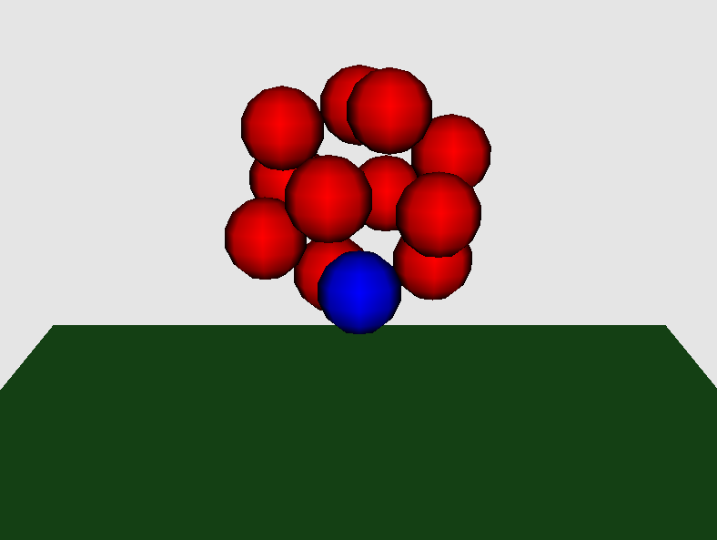
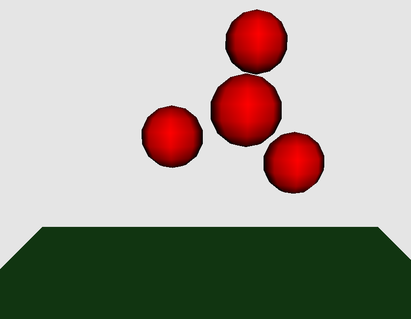
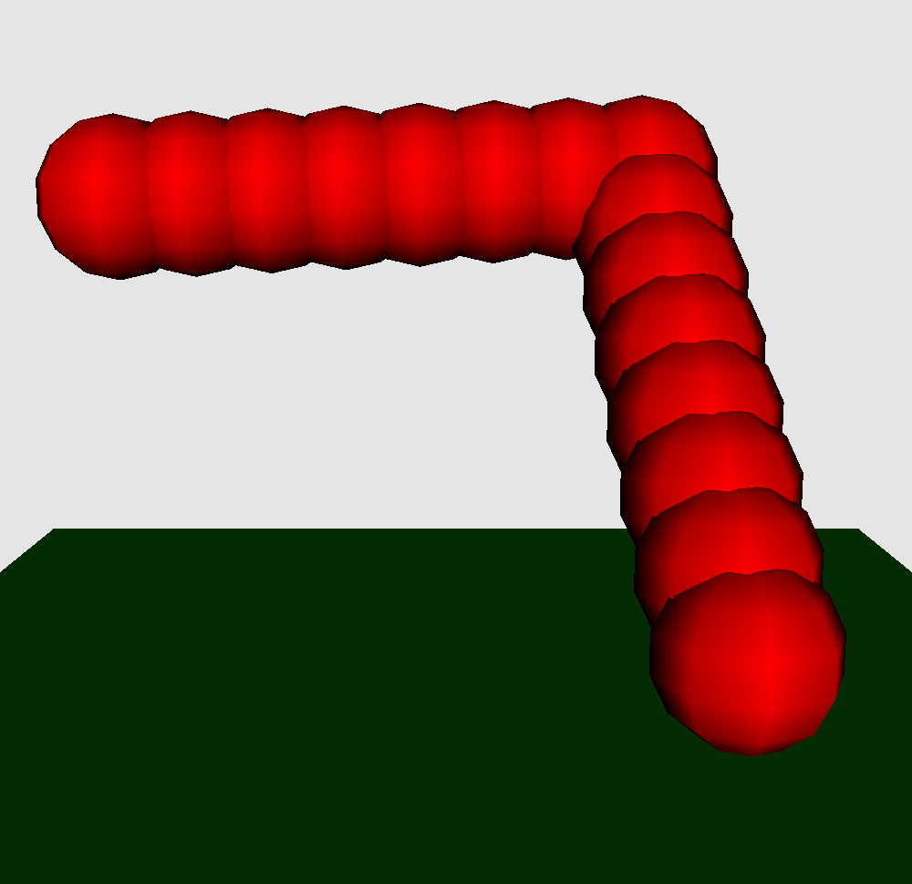
Figure 1: Rigid multiblob models of three types of particles studied in this work. The blobs are shown as red spheres of radius equal to the blob hydrodynamic radius, and the no-slip bottom wall is shown as a green plane. (Left) A spherical colloidal “surfer” that has a much denser metallic cube of hematite embedded in it, taken from the work of Palacci et al. Hematites_Science . In our computer simulations we model this as an icosahedron of rigidly-connected blobs, one of which (indicated by a blue sphere) models the dense hematite and holds all of the mass of the particle. (Middle) A tetramer formed by connecting four colloidal particles using DNA bonding into a tetrahedron, as in the work of Kraft et al. ComplexShapeColloids . The multiblob model has four blobs rigidly placed at the vertices of a tetrahedron. (Right) A right-angle boomerang colloid manufactured using lithography and studied in a slit channel formed by two microscope slides by Chakrabarty et al. BoomerangDiffusion , modeled here using a 15-blob approximation.

For the purposes of hydrodynamic calculations, we discretize rigid bodies by constructing them out of multiple rigidly-connected spherical “blobs” of hydrodynamic radius $a$. These blobs can be thought of as hydrodynamically minimally-resolved spheres forming a rigid conglomerate that approximates the hydrodynamics of the actual rigid object being studied. Examples of such “multiblob” MultiblobSprings models of several types of rigid bodies studied in recent experiments are given in Fig. 1. As Fig. 2 illustrates for a rigid sphere, the hydrodynamic fidelity of rigid multiblob MultiblobSprings models can be refined by increasing the number of blobs (and decreasing their hydrodynamic radius $a$ accordingly); of course, increasing the resolution comes at a significant increase in the computational cost of the method. Similar “bead” or “raspberry” models appear in a number of studies of hydrodynamics of particle suspensions HYDROPRO ; HYDROPRO_Globular ; RotationalBD_Torre ; Raspberry_MPCD ; Raspberry_LBM ; SPM_Rigid ; StokesianDynamics_Rigid ; HYDROLIB ; SphereConglomerate ; RigidBody_SD ; IBM_Sphere ; MultiblobSprings , with the blobs or beads being either connected rigidly as we do here, or connected via stiff springs; in some models the fluid or particle inertia is included also. Since in this work we focus on the long-time diffusive dynamics it is crucial to use rigid rather than stiff springs, and to eliminate inertia in the spirit of the overdamped approximation, in order to allow for a sufficiently large time step to reach physical time scales of interest (seconds to minutes in actual experiments).

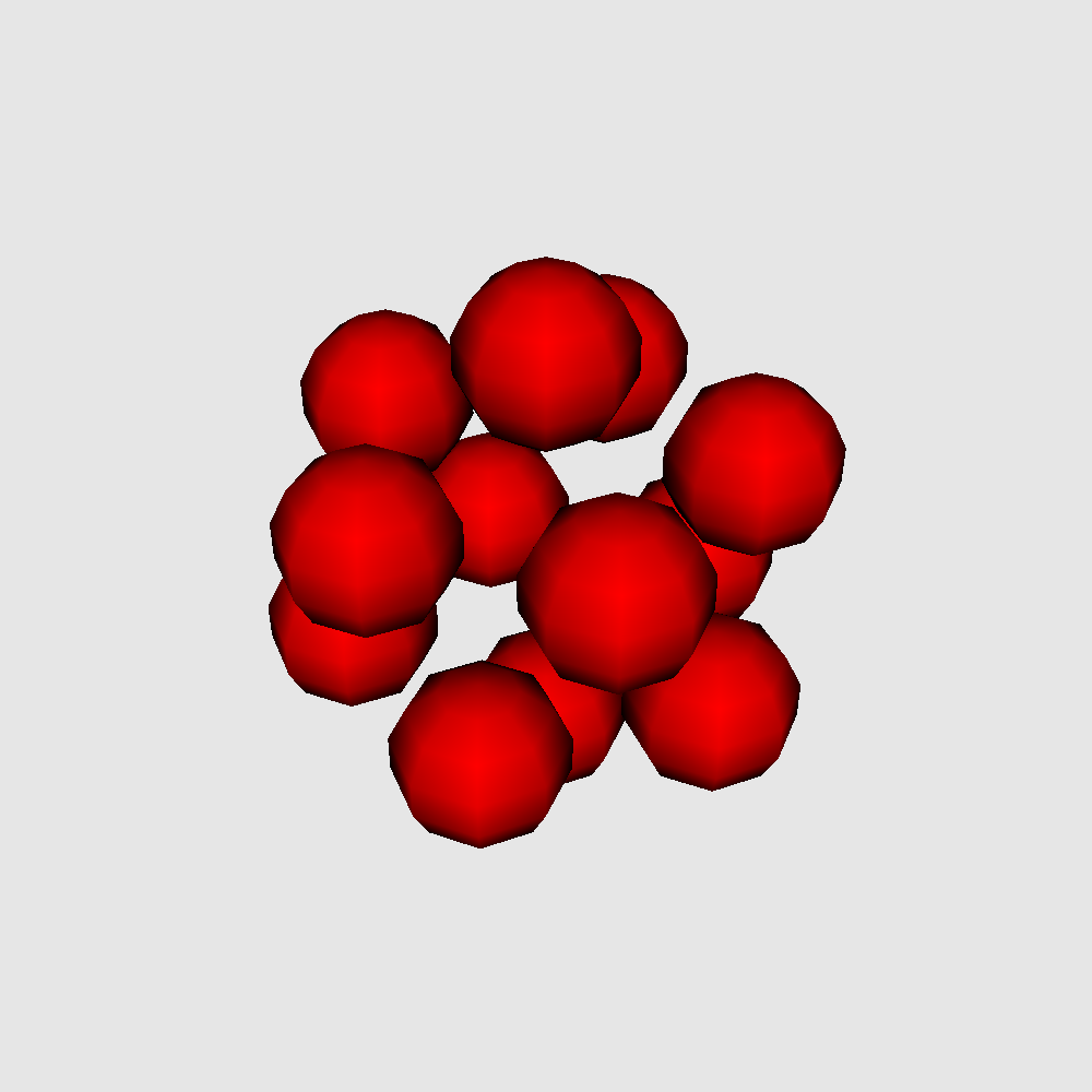
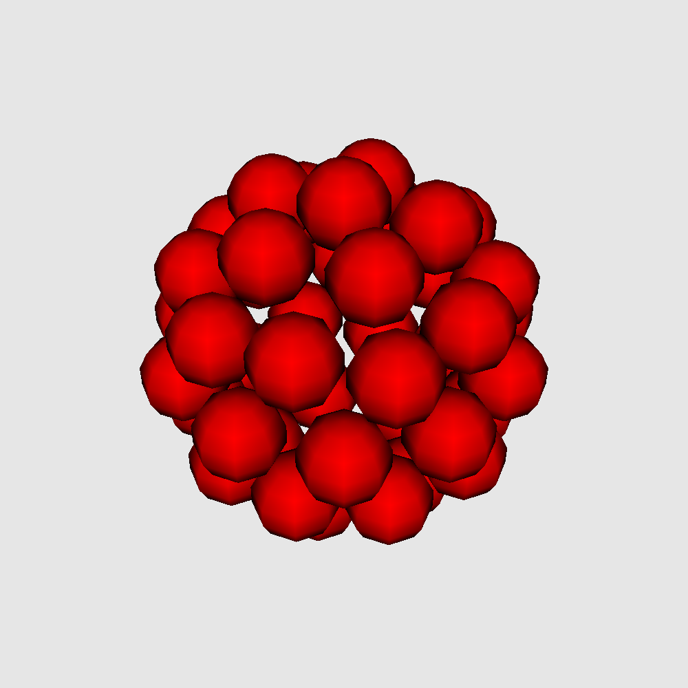
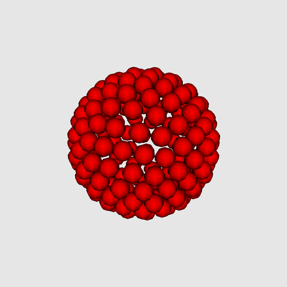
Figure 2: Rigid multiblob or “raspberry” models of a rigid sphere, containing 12 blobs (left), 42 blobs (center), or 162 blobs (right) placed on the surface of a sphere using a recursive triangulation procedure starting from an icosahedron (left-most panel). The radius of the red spheres is equal to the effective hydrodynamic radius of a blob; the hydrodynamic radius of the resulting rigid multiblob sphere is computed numerically MultiblobSprings ; RigidIBM and is generally larger than the geometric radius of the sphere used for the recursive triangulation.

After discretizing a rigid body using $n$ blobs, we write down a system of equations that constrain the blobs to move rigidly. These intuitive equations are written in a large number of prior works HYDROPRO ; HYDROPRO_Globular ; RotationalBD_Torre ; StokesianDynamics_Rigid ; HYDROLIB ; SphereConglomerate ; RigidBody_SD ; RegularizedStokeslets but we refer to StokesianDynamics_Rigid for a clear yet detailed exposition; the authors also provide associated computer codes (not used in this work) in the supplementary material. Letting $\boldsymbol{\lambda}=\left\{\boldsymbol{\lambda}_{1},\ldots,\boldsymbol{\lambda}_{n}\right\}$ be a vector of forces (Lagrange multipliers) that act on each blob to enforce the rigidity of the body, we have the linear system for $\boldsymbol{\lambda}$, $\boldsymbol{u}$ and $\boldsymbol{\omega}$,

$$\sum_{j}\left(\boldsymbol{M}_{B}\right)_{ij}\boldsymbol{\lambda}_{j}= \boldsymbol{u}+\boldsymbol{\omega}\times(\boldsymbol{r}_{i}-\boldsymbol{q}),\quad\forall i$$ (72)

$$\sum_{i}\boldsymbol{\lambda}_{i}= \boldsymbol{F}$$

$$\sum_{i}(\boldsymbol{r}_{i}-\boldsymbol{q})\times\boldsymbol{\lambda}_{i}= \boldsymbol{\tau},$$

where $\boldsymbol{u}$ is the velocity of the tracking point $\boldsymbol{q}$, $\boldsymbol{\omega}$ is the angular velocity of the body around $\boldsymbol{q}$, $\boldsymbol{F}$ is the total force applied on the body, $\boldsymbol{\tau}$ is the total torque applied to the body about point $\boldsymbol{q}$, and $\boldsymbol{r}_{i}$ is the position of blob $i$.

Here the blob-blob translational mobility $\boldsymbol{M}_{B}$ describes the hydrodynamic relations between the blobs, accounting for the influence of the boundaries. The $d\times d$ block of the translational mobility $\left(\boldsymbol{M}_{B}\right)_{ij}$ computes the velocity of blob $i$ given forces on blob $j$, neglecting the presence of the other blobs in a pairwise approximation. In the presence of a single wall, an analytic approximation to $\left(\boldsymbol{M}_{B}\right)_{ij}$ is given by Swan and Brady StokesianDynamics_Wall , as a generalization of the Rotne-Prager (RP) tensor RotnePrager to account for the no-slip boundary using Blake’s image construction. In this work we utilize the translation-translation part of the Rotne-Prager-Blake mobility given by Eqs. (B1) and (C2) in StokesianDynamics_Wall to compute $\boldsymbol{M}_{B}$, ignoring the higher order torque and stresslet terms in the spirit of the minimally-resolved blob model BrownianBlobs . The self-mobilities for a single blob are given in (94) in Appendix D. Note that in a suitable limit of infinitely many blobs of appropriate radius, solving (72) computes the exact grand mobility for the rigid body (or a collection of bodies), even though only a low-order RP-like approximation is used for $\boldsymbol{M}_{B}$ RigidIBM ; RegularizedStokeslets . To see this, note that blob methods can be considered as a discretization of a regularized first-kind integral equation RegularizedStokeslets for the Stokes flow around the rigid bodies. In a recent experimental and computational study TetheredNanowires , the mobility of a rigid rod tethered to a hard wall was computed using the multiblob approach as we do here, however, in that work the wall was created from (many) blobs instead of using the known generalization of the RP tensor to a single-wall geometry StokesianDynamics_Wall as we do here.

The solution of the linear system (72) defines a linear mapping from applied force and torque to body velocity and angular velocity, and thus gives the grand mobility $\boldsymbol{N}$ (for explicit formulas, see StokesianDynamics_Rigid ). Observe that generalizing the system (72) to a collection of rigid bodies is trivial. In the examples considered in the work, the number of blobs is small and the system (72) can easily be solved by computing the Schur complement StokesianDynamics_Rigid and inverting it directly with dense linear algebra. The use of dense linear algebra allows us to focus our attention on the temporal integrators for the overdamped dynamics and not on linear algebra or hydrodynamics issues. In principle, our temporal integrators can be used with a variety of methods for computing the hydrodynamic mobility of suspensions of rigid bodies, for example, boundary-integral or boundary-element methods can be used to compute the (action of the) grand mobility with higher accuracy.

We compute the square root $\boldsymbol{N}^{\frac{1}{2}}$ by performing a dense Cholesky factorization on $\boldsymbol{N}$. It is important to note that if $\boldsymbol{M}_{B}$ is SPD, the grand mobility $\boldsymbol{N}$ computed by solving (72) is also SPD. Note that the Swan-Brady approximation to $\boldsymbol{M}_{B}$ StokesianDynamics_Wall used here is based on the Rotne-Prager tensor and is thus only guaranteed to be positive definite when the blobs do not overlap each other or the wall, i.e., when no two blobs are closer than a distance $2a$ and the distance of all blob centroids to the wall is greater than $a$. It is possible to generalize the Rotne-Prager-Yamakawa tensor to confined systems RPY_Shear_Wall , thus guaranteeing an SPD $\boldsymbol{M}_{B}$ even when blobs overlap each other or the wall (but of course their centroids must remain above the wall), but we know of no published explicit formula that accomplishes this even for the case of a single wall. Fortunately, for our model of boomerang-shaped particles we numerically observe an SPD mobility when the blobs do not overlap the wall even though blobs overlap each other.

IV.3 Colloidal tetramer: Tetrahedron

In this section we study a tetramer formed by rigidly connecting four colloidal spheres at the vertices of a tetrahedron ComplexShapeColloids ; ColloidalClusters_Granick , diffusing near a single no-slip boundary. The tetrahedron is discretized in a minimally-resolved way using 4 blobs, one at each vertex of a regular tetrahedron, as illustrated in the pictured in the left panel of Fig. 1. In some arbitrary units, each blob is a distance $d=2$ away from all of the others and has a hydrodynamic radius of $a=0.5$; this somewhat arbitrary choice makes the tetrahedron hydrodynamically sufficiently different from a sphere to require resolving the orientation of the body as well.

To avoid symmetries and make the test more general, we assume each of the four spheres to have a different density; the gravitational forces on the vertices in the negative $z$ direction are set to $F_{1}=0.15$, $F_{2}=0.1$, $F_{3}=0.3$ and $F_{4}=0.05$ in units of $k_{B}T/a$. To prevent the tetrahedron from passing through the wall, we include a repulsive potential (73) between each of the blobs and the wall, based on an ad-hoc combination of a Yukawa and a hard-sphere-like divergent potential,

$$U_{\mbox{wall}}(h;\,a)= \frac{\epsilon a}{h-a}\,\exp\left(-\frac{h-a}{b}\right),$$ (73)

where $h$ is the height of the center of the blob above the wall, $\epsilon=20k_{B}T$ is the repulsion strength, and $b=0.5a$ to be the Debye length (these values are selected somewhat arbitrarily). The total force and torque on the rigid tetramer is the sum of the forces and torques on the individual blobs. The above choice of parameters gives the center of the tetrahedron a gravitational height (70) of $h_{g}\approx 1.75a$.

For comparison and validation, we also construct an approximation to the freely-moving rigid tetrahedron using four blobs connected by stiff springs, and then employ the FIB method BrownianBlobs to simulate the diffusive motion of the almost-rigid tetramer; the same parameters are used in both simulations. The FIB simulation was performed in a domain of $64\times 64\times 64$ grid cells of width $\Delta x=0.796a$ using the 4-point Peskin kernel, which ensures that the effective hydrodynamic radius of the blobs is $a$ BrownianBlobs . The boundaries on the top and bottom of the domain are both no-slip walls, which differs from the domain for the rigid body simulations, but since the center of the tetrahedron almost never goes past $20\%$ of the channel width (see figure 3), the effect of the top wall is relatively minor. The spring stiffness was set to $k=200\,k_{B}T/a$ to keep the deformations of the tetrahedron small; this imposes a stringent limit on the time step size $\Delta t$.

IV.3.1 Equilibrium Distribution

In this section we examine the equilibrium distribution for the colloidal tetramer. We use a Monte Carlo method to generate the marginal Gibbs-Boltzmann distribution for the height of the geometric center of the tetrahedron, and compare to our numerical results. We see in Fig. 3 that the Fixman (41) and RFD schemes (48) are in good agreement with the Gibbs-Boltzmann distribution. The Euler-Maruyama scheme (37), with the obvious additions to include translation, however, neglects parts of the stochastic drift and generates an equilibrium distribution which has clear errors that do not vanish as the time step size is refined (not shown).

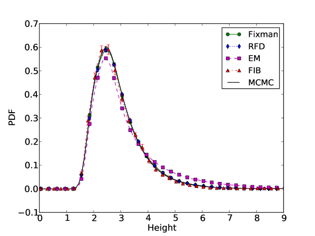
Figure 3: Equilibrium distribution for the height of the geometric center of the tetramer colloid pictured in the left panel of Fig. 1. The results obtained by using the FIB method and the Fixman (Section III.2) and RFD (Section III.3) integratrors agree with the Gibbs-Boltzmann distribution generated using Monte Carlo sampling. The results obtained by using the inconsistent EM scheme (37) demonstrate that neglecting the stochastic drift term yields an incorrect equilibrium distribution. This plot is based on 16 runs of $3\cdot 10^{5}$ time steps with a small time step size of $\Delta t\approx 0.0653\,\left(6\pi\eta a^{3}/k_{B}T\right)$; no rejections were needed for this small time step in any of the runs.

IV.3.2 Mean Square Displacement

In this section, we examine the translational mean square displacement of the tetrahedron. In the left panel of Fig. 4 we examine the effect of the choice of tracking point on the parallel mean square displacement by comparing $D_{\parallel}\left(\tau\right)$ when tracking the geometric center of the tetrahedron, versus tracking one of the four vertices. In both cases (56) gives the initial slope of the MSD as it must, and these slopes are clearly different. Since at long times the slopes of the parallel MSD is independent of the choice of tracking point, the MSD cannot be linear at all times for both choices of tracking point. Indeed, the results in Fig. 4 show that the parallel MSD is linear to within statistical and numerical truncation errors only when the geometric center is tracked. By contrast, the rotational MSD is insensitive to the choice of tracking point, as seen in the right panel of Fig. 4.

We note that far from the wall, torques applied about the center of the tetrahedron generate no translation, indicating that in the absence of confinement the geometric center is both the CoM and the exact three dimensional CoH (which does not exist for general rigid bodies). In the presence of the boundary, this is not strictly the case, but we nonetheless observe in Fig. 4 that the average parallel mobility evaluated using the center of the tetrahedron as an origin gives a good approximation to the long time quasi two-dimensional diffusion coefficient $\chi_{2D}$. This is perhaps not surprising due to the high symmetry of a tetrahedron, as the geometric center is the “obvious” point to track.

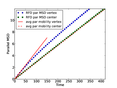
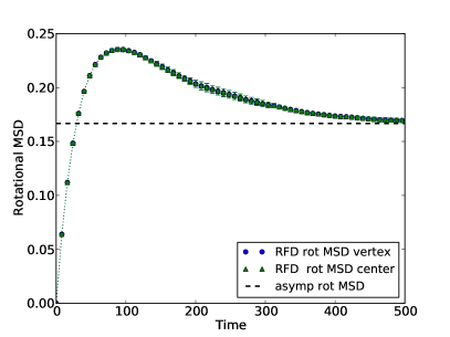
Figure 4: Mean square displacement for a colloidal tetramer sedimented near a bottom wall. The data for both figures is generated from 4 independent runs of $3\cdot 10^{5}$ time steps with a time step size of $\Delta t\approx 0.136\,\left(6\pi\eta a^{3}/k_{B}T\right)$; the highest rejection rate was $2.33\times 10^{-5}$ (a total of 7 rejections). The MSDs for each tracking point are calculated from the same trajectories. (Left) Comparison of parallel translational MSD $D_{\parallel}\left(\tau\right)$ when tracking the geometric center (green squares), versus when tracking the fourth vertex (blue squares). We see that at short times the numerical slope agrees with (56), shown as a red dashed line of slope $1.34(k_{B}T/6\pi\eta a)\approx 2.8\cdot 10^{-2}$ for the geometric center, and as a red solid line of slope $2.21(k_{B}T/6\pi\eta a)\approx 4.7\cdot 10^{-2}$ for the vertex. (Right) Comparison of the parallel ($(x-x)$ or $(y-y)$) component of the rotational mean square displacement using the two choices of tracking point. The asymptotic rotational MSD predicted by (71) is shown as a dashed line.

In Figure 5 we compare results for the MSD obtained using the overdamped rigid-body integrators from Section III to results obtained using the FIB method and stiff springs. We examine the mean square translational displacement parallel and perpendicular to the wall, as well as the rotational MSD, and find that the behavior of the tetrahedron is the same for both the stiff and rigid simulations; this provides a validation of our rigid-body methods and our codes. However, due to the presence of the stiff springs, using the FIB method to simulate a rigid body requires a time step size that is 32 times shorter. Due to the small time step size required for the tetrahedron constructed using rigid springs, and the high cost of numerically solving a Stokes problem each time step, it is computationally impractical to study the long time diffusion coefficient using the FIB method. The time step size for the rigid-body method could in principle be even larger and still resolve the dynamics of the body, but it is limited by the stiff potential used to repel the particle from the wall; we keep $\Delta t$ sufficiently small to strictly control the number of rejections of unphysical states where a blob gets too close to or passes through the wall. In Section V we discuss some ideas that may allow for the use of larger time step sizes even in the presence of steep repulsive forces.

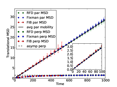
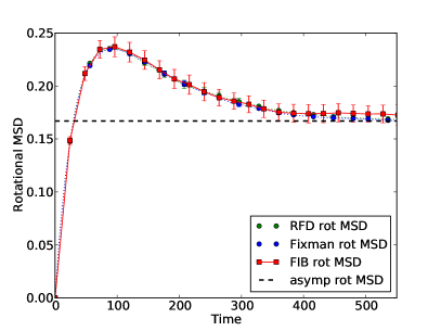
Figure 5: Comparison of the mean square displacement for a colloidal tetramer sedimented near a bottom wall, obtained by treating the body as rigid using the RFD and Fixman methods developed here (see caption of Fig. 4), versus keeping it nearly rigid with stiff springs and using the FIB method BrownianBlobs . For the FIB runs we used 32 simulations of $10^{5}$ time steps each, with a time step size 32 times smaller than in the rigid-body simulations. (Left) Parallel translational MSD when tracking the geometric center of the tetrahedron. The inset focuses on the short time diffusion, and shows a slight hydrodynamic difference between the rigid and semi-rigid models that is due to the different methods used to handle the hydrodynamics, as well as the slight flexibility of the tetrahedron in the FIB simulations. (Right) The parallel ($(x-x)$ or $(y-y)$) component of the rotational MSD (22).

IV.4 Asymmetric sphere: Icosahedron

In this section we examine the diffusive motion of a rigid sphere whose center of mass is displaced away from the geometric center, in the presence of gravity and a bottom wall (no-slip boundary). This models recently manufactured colloidal “surfers” that become active when the particles sediment to a microscope slide Hematites_Science ; here we consider a passive particle in the absence of chemical driving forces. Diffusive and rotational dynamics of a symmetric patterned (Janus) sphere near a boundary has been studied experimentally by Anthony et al. SphereNearWall , and can be described well by theoretical approximations for the mobility of a rigid sphere near a planar wall BrennerBook .

We construct a hydrodynamic model of an asymmetric rigid sphere of radius $a_{I}$ by rigidly constraining 12 blobs at the vertices of an icosahedron; a similar blob model of a sphere was used in Ref. MultiblobSprings but was based on (stiff) penalty springs rather than rigid-body constraints. Note that more accurate results can be obtained by using more blobs to construct the spherical shell RigidIBM . Each blob has a hydrodynamics radius of $a=0.175$ and is located a distance $2.5a$ from the center of the icosahedron, so that the minimal distance between two blobs is about $2.63a$. These parameters are chosen so that the icosahedron is hydrodynamically nearly rotationally invariant, and has an effective translational hydrodynamic radius (computed numerically) in bulk (i.e., far from the wall) of

$$a_{I}= \frac{1}{6\pi\eta\left(\mbox{Tr}\left(\boldsymbol{M}_{\boldsymbol{u}\boldsymbol{F}}\right)/3\right)}\approx 2.86a=0.5,$$

in some arbitrary units. A gravitational force of $F=0.5=1.25\,k_{B}T/a_{I}$ is applied to one of the 12 blobs, which represents the dense hematite cube embedded in the nearly spherical colloidal surfers of Palacci et al. Hematites_Science . Gravity therefore generates a torque around the center of the sphere and causes the icosahedron to prefer orientations where the heavy blob is facing down. A short-ranged repulsive force $U\left(h;\,a_{I}\right)$ given by (73) is added to keep the icosahedron from overlapping the wall, where now $h$ is the distance from the center of the icosahedron to the wall, the repulsion strength is $\epsilon=20k_{B}T$, and the Debye length is (arbitrarily) set to $b=a_{I}$. This choice of parameters gives the center of the icosahedron a gravitational height (70) of $h_{g}\approx 0.96a_{I}$. Note that in this example the icosahedron is considered to be a hydrodynamic approximation of a physical sphere and therefore the repulsive force acts on the center of the sphere (thus not generating any torque), rather than acting on each of the 12 blobs individually (which would generate some small spurious torque).

IV.4.1 Equilibrium Distribution

We first investigate the equilbrium distribution $P_{eq}\left(\boldsymbol{q},\boldsymbol{\theta}\right)$, examining the marginal distributions of height $h$ and orientation angle $\theta$, which is the angle between the $z$ axis and the vector connecting the center of the icosahedron to the blob to which we apply the gravitational force. In this simple example, we can compute the marginals of the equilibrium Gibbs-Boltzmann distribution analytically for both $h$ and $\theta$, and they are compared to numerical results in Fig. 6. We see that the RFD and Fixman schemes agree with each other and with theory. Due to the nonuniform gravitational forcing on the icosahedron, it prefers orientations with $\theta$ closer to zero, but the thermal fluctuations causes it to explore all orientations.

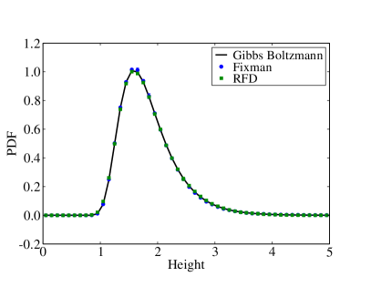
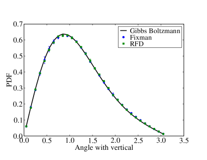
Figure 6: Equilibrium distribution for a rigid icosahedron of blobs compared to analytic expressions for the Gibbs-Boltzmann distribution. These figures were created using data from 6 independent runs of $4\cdot 10^{5}$ time steps with a small time step size of $\Delta t=0.04\,(6\pi\eta a_{I}^{3})/k_{B}T$ to avoid rejections; no rejections occurred during these simulations. (Left) Equilibrium distribution of the height $h$, the distance from the center of the icosahedron to the wall. (Right) Equilibrium distribution of the angle $\theta$, where $\theta=0$ indicates that the heavy blob is at the bottom of the icosahedron, and $\theta=\pi$ indicates that it is at the top. As expected, we see the distribution skewed towards smaller values of $\theta$ due to the gravitational force.

IV.4.2 Mean Square Displacement

To validate how well our scheme captures the dynamics of the system, we examine the mean square displacement of the geometric center of the icosahedron. In Fig. 7 we compare our results to the mean square displacement of an actual hard sphere with hydrodynamic radius $a=0.5.$ We apply torques and forces to the sphere that are identical to those applied to the icosahedron, but for the hydrodynamic mobility of the sphere we use the most accurate theoretical expressions available in the literature, see (95,96,97) in Appendix D, instead of relying on the blob approximation to a sphere (94), even though in this specific case (94) is sufficiently accurate. This tests allows us to both evaluate our temporal integration method, as well as to examine how well the 12-bead model approximates a single spherical particle.

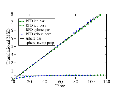
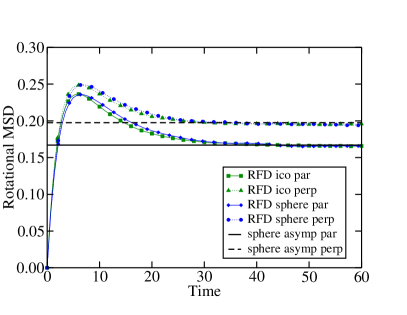
Figure 7: Mean square displacements for a sphere with nonuniform mass distribution diffusing near a planar boundary. Symbols show numerical results obtained by processing long equilibrium trajectories, while lines show theoretical predictions. These figures were generated using data from 16 independent trajectories of length $5\cdot 10^{5}$ time steps, using the RDF temporal integrator with a small time step size of $\Delta t=0.004\>(6\pi\eta a_{I}^{3})/k_{B}T$ to eliminate rejections. (Left) Parallel ($D_{\parallel}(\tau)$) and perpendicular ($D_{\perp}(\tau)$) translational MSD of a rigid icosahedron of blobs. The solid black line shows the theoretical parallel translational MSD predicted by (68) for a rigid sphere using the best-known approximations to the hydrodynamic mobility (95,96,97), while the dashed black line shows the asymptotic perpendicular translational MSD (69). As expected, the icosahedron behaves like a sphere with equal effective hydrodynamic radius MultiblobSprings . (Right) Parallel ($x-x$ or $y-y$) as well as perpendicular ($z-z$) components of the rotational mean square displacement (58). The dashed line shows the asymptotic rotational MSD (71). We see that the rotational dynamics of the rigid icosahedron and a true sphere are also in good agreement.

The results shown in Fig. 7 demonstrate that the dynamics of the icosahedral rigid multiblob is essentially identical to that of an actual sphere. Note that for a sphere the mobility does not depend on the orientation of the sphere. Furthermore, by symmetry, the gravitational force (perpendicular to the wall) cannot induce rotation of the sphere, and by symmetry, a torque cannot introduce vertical displacements. Because of these special symmetries the parallel MSD is linear for all times and therefore (68) gives the long-time quasi two-dimensional diffusion coefficient $\chi_{2D}$; this has in fact been confirmed experimentally with relatively good accuracy for spheres whose center of mass is very close to their geometric center SphereNearWall .

IV.5 Colloidal Boomerang

The authors of reference BoomerangDiffusion perform a detailed experimental study of the quasi-two-dimensional translational and rotational diffusion of lithographed symmetric right-angle boomerang colloids (see the right panel of Fig. 2) confined between two closely-spaced microscope slides. Subsequently this work was extended to asymmetric (L-shaped) right-angle boomerangs AsymmetricBoomerangs as well as non-right-angle boomerangs angleBoomerangs . Some theoretical analysis is also performed assuming that the overdamped dynamics of the particles is strictly two-dimensional. Of course, the actual dynamics of the particles is three dimensional, and a complete theoretical or numerical analysis of the diffusive dynamics requires the complete formalism developed in this paper.

In this section we examine a single symmetric right-angle boomerang near a single no-slip boundary (bottom wall) in the presence of gravity. We choose to study a single boundary rather than a slit channel as done in the experiments in order to simplify the hydrodynamic calculations of mobilities StokesianDynamics_Wall ; in principle one can construct tabulated approximations of self and pairwise mobilities in a slit channel but this is quite complex and expensive StokesianDynamics_Slit . While we cannot make direct comparisons with the experimental values reported in Ref. BoomerangDiffusion in this work, we can still address the fundamental questions about differences between fully three-dimensional and quasi two-dimensional diffusion. Specifically, by enlarging the gravitational force we apply to the boomerang (i.e., increasing its effective density mismatch with the solvent), we can cause the motion to be more or less confined to a two dimensional plane parallel to the bottom wall. In this section we use microns as the unit of length, seconds as the unit of time, and milligrams as the unit of mass.

For hydrodynamic calculations, we construct a blob model of a boomerang and try to match the physical parameters in the experiments BoomerangDiffusion as close as possible. Our model of the boomerang particle is constructed by rigidly connecting 15 blobs, one at the cross point, and 7 for each arm, as illustrated in the right panel in Fig. 1. Prior investigations in the context of the immersed boundary method IBM_Sphere , which we have also confirmed independently by using the Rotne-Prager tensor as the pairwise blob mobility, have shown that to construct a good hydrodynamic approximation of a rigid cylinder of radius $r$ using blobs, one should set the effective hydrodynamic radius of each blob to $a\approx\sqrt{3/2}\,r$, and place the blobs centers on a line at a distance of around $a$ (the precise value does not matter much). Following these recommendations, we set the blob radius to $a=0.325$, which gives an effective cylinder radius of 0.265, and the blobs are spaced a distance 0.3 apart. Note that in this minimally-resolved blob model the cross-section of the arms of the boomerang is cylindrical rather than square, as would be more realistic for modeling the lithographed particles. We have, however, compared to a more resolved 120-blob model constructed from the initial boomerang by replacing each of its 15 blobs by 8 smaller blobs of radius $0.1625$ placed at the vertices of a rectangular prism of size $0.15\times 0.285\times 0.245$ centered at the location of the original blob. We find only minor differences with the minimally-resolved model, for example, in bulk (without confinement) the diffusion coefficients in the plane of the boomerang are computed to be (in units of $\mu m^{2}/s$) $0.243$ and $0.283$ for the 15-blob model, and $0.245$ and $0.291$ for the 120-blob model.

For a free boomerang far away from boundaries, there is a unique CoM that, due to symmetry, must lie on the the line that bisects the boomerang arms. Also, there must be a unique point on the bisector for which there is no coupling between torque applied out of the plane of the boomerang and the translational motion in the plane of the boomerang. We can consider this point as the CoH for quasi-two-dimensional diffusion BoomerangDiffusion , although, as already explained, this point is not a CoH in the strict sense for three-dimensional diffusion. The locations of the bulk CoM and the bulk quasi-two-dimensional CoH, which we shall henceforth imprecisely refer to as just CoM and CoH, can be computed from (64) and (65), respectively. For our blob model, we compute the CoH to be is about 1.08 microns away from the cross point (center of the intersection blob), and the CoM is 0.96 microns from the cross point; we get the same estimates from the more refined 120-blob models. These numbers compare favorably to the experimental findings in BoomerangDiffusion , where the CoH is estimated to be a distance of 1.16 microns from the cross point; the CoM is not mentioned in the experimental works on boomerang particles. The difference between the CoH and CoM is too small for this specific particle shape for us to be able to tell the difference to within statistical errors; in future work we will look for other planar particle shapes for which the difference may be more significant and measurable in both simulations and experiments.

The total gravitational force applied to the body is $0.18\times g\,\left(k_{B}T/a\right)$ where $g$ is a parameter that we vary; we split the gravitational force evenly among the 15 blobs. Here $g=1$ gives a rough approximation of the gravitational binding experienced by the actual lithographed particles, which have a density of $1.2\,\mbox{g}/\mbox{cm}^{3}$. Each blob is also repelled from the wall using the potential (73) with screening length $b=0.5a$ and strength $\epsilon=23.08kT$. The gravitational height (70) for one of the two (equivalent) tips of the boomerang are shown in Table 1 for several values of $g$. Since the tips are the points that are most likely to venture further from the wall, these values give an indication of how close to two-dimensional the dynamics of the boomerang is.

IV.5.1 Translational Diffusion

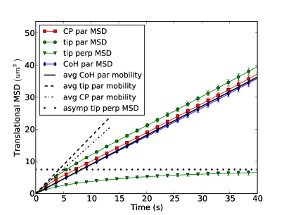
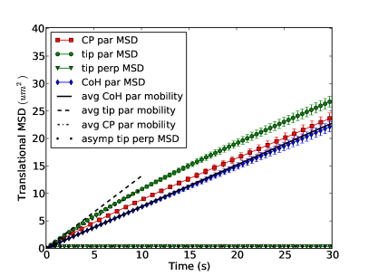
Figure 8: Translational MSD of a right-angle symmetric boomerang for gravity $g=1$ (left panel) and $g=20$ (right panel) parallel and perpendicular to the wall, see legend. The same trajectories are used but the parallel MSD is computed using three different choices of the tracking point: cross point (CP) at the corner of the right angle, (one of the) tip(s) of the boomerang, and the center of hydrodynamic stress (CoH), which we note is essentially indistinguishable for this purpose from the center of mobility (CoM). For the perpendicular MSD we only show the results for the tip and show the expected asymptotic value with a dotted line. The slopes of the parallel MSD at the origin are shown with lines (see legend) and estimated using Monte Carlo sampling via (68). We see that by calculating the MSD tracking the CoH/CoM, the MSD is essentially linear with time, and therefore the short time diffusion coefficient (68) matches the (unique) long time diffusion coefficient $\chi_{2D}$. This is not the case when tracking the cross point or the tip of one of the arms.

In Fig. 8 we show the parallel and perpendicular translational MSDs of the boomerang for a weak ($g=1$, left panel) and a strong gravitational sedimentation ($g=20$, right panel), where strong here means that the gravity is sufficiently strong to keep the boomerang essentially flat against the surface. For the parallel MSD, we show results based on three different choices of the tracking point: 1) the CoH, or in this example, equivalently the CoM; 2) the center of the blob at the tip of one of the arms; and 3) the cross point (CP), which is the center of the blob at the cross point where the arms meet. For an unconfined boomerang, we expect that the parallel MSD measured using the CoM will be strictly linear in time. We also expect that for the boomerang confined to a plane by strong gravity and exhibiting quasi two-dimensional diffusion, the MSD will be linear in time when tracking the CoH BoomerangDiffusion ; AsymmetricBoomerangs . However, in our simulations, we find that due to the close proximity of the CoH and the CoM, the MSD is identical to within statistical error independent of which of these two points was tracked. For clarity, we only include the MSD calculated from the CoH in our results, with the understanding that the CoM is indistinguishable at this level of accuracy. We see from the figure that by choosing the CoH as the tracking point, we obtain a MSD that is linear over all times up to statistical accuracy for both gravities. This means that we can get an accurate estimate of the long-time diffusion coefficient $\chi_{2D}$ by using equation (68) over a broad range of gravities. This statement should, however, be checked for other particle shapes for which the CoH and CoM are sufficiently far apart, before drawing broad conclusions.

$g$	$\chi_{2D}(\mu m^{2}/s)$	$\chi_{2D}/\chi_{3D}$	$\chi_{\theta}\left(\mbox{rad}^{2}/s\right)$	$h_{g}(\mu m)$	$\chi_{2D}/\chi_{3D}$ sphere
$1$	0.226	0.834	1.42	1.77	0.837
$10$	0.194	0.716	0.79	0.605	0.724
$20$	0.185	0.683	0.22	0.419	0.680

Table 1: Long-time quasi two-dimensional diffusion coefficient $\chi_{2D}$ for the boomerang colloid at $g=1,\,10,$ and $20$ estimated using (68) and tracking the CoH. The diffusion coefficient for a free boomerang in an unbounded fluid $\chi_{3D}$ is computed using (67). The rotational diffusion coefficient $\chi_{\theta}$ is calculated using (93). Comparing the effective gravitational heights (70), calculated for the tip of the boomerang, and the boomerang’s arm length ($2.1\mu m$) or the blob radius ($0.325\mu m$) gives an indication of how flat the boomerang is against the wall. In the last column we estimate the reduction in mobility relative to bulk for a sphere of the same radius as the blobs and at the same gravitational height as the tip of the boomerang.

In Table 1 we show the estimated long-time parallel diffusion coefficient $\chi_{2D}$ obtained from (68) for different strengths of the gravitational sedimentation. We find that, perhaps surprisingly, the presence of the boundary does not strongly reduce the effective short-time diffusion coefficient compared to bulk, except at the largest gravity. In the last column of the table we give the corresponding reduction in mobility for a sphere of the same radius as the blob radius, as obtained from the theoretical estimate (97) averaged against a Gibbs-Boltzmann distribution $\sim\exp\left(-h/h_{g}\right)$ for the height above the wall; a remarkable agreement is observed despite the significant difference in the particle shape. The value of the quasi two dimensional diffusion coefficient is measured experimentally in Ref. BoomerangDiffusion for the case of a boomerang particle confined between two microscope slides a distance $2\mu m$ apart, and a value of $\chi_{2D}^{\mbox{exp }}=0.054\,\mu m^{2}/s$ is reported. This is lower than the values calculated here, which we expect is largely due to the absence of the top wall in our simulations, which will significantly increase the drag on the boomerang for such strong confinement.

IV.5.2 Rotational Diffusion

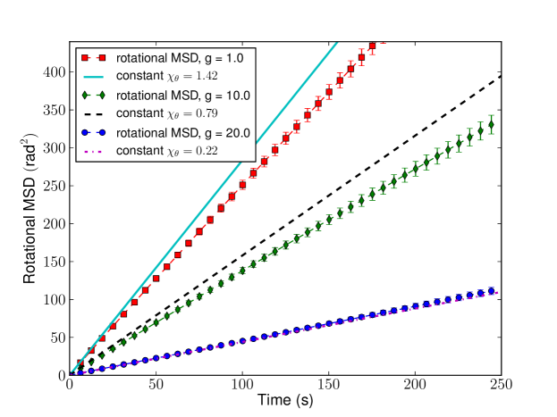
Figure 9: Planar rotational mean squared displacement (74) of the colloidal boomerang for three different strengths of the gravitational confinement.

To estimate the quasi-two-dimensional rotational diffusion coefficient $\chi_{\theta}$, measured experimentally in Ref. BoomerangDiffusion , we project the bisector of the boomerang arms into the $x-y$ plane, and define $\theta(t)$ to be the angle of rotation around the $z$ axis between this projected vector at time $t$ and the initial projected bisector. We count each full counterclockwise rotation as an addition of $2\pi$, and similarly we subtract $2\pi$ for each full clockwise rotation, allowing the value of $\theta$ to take values in all of $\mathbb{R}$. Truly two-dimensional rotational diffusion (where the colloid stays in the $x-y$ plane) corresponds to $\theta(t)$ being standard Brownian motion. We define a planar rotational mean square displacement from increments of the angle $\theta$,

$$D_{\theta}\left(\tau\right)=\left\langle\Delta\theta^{2}\right\rangle=\left\langle\left(\theta(t+\tau)-\theta(t)\right)^{2}\right\rangle.$$ (74)

In Fig. 9 we show numerical results for $D_{\theta}\left(\tau\right)$. We see that for $g=20$, when the boomerang is most flat, the quantity $D_{\theta}$ is linear in time for all times to within statistical error bars, while for lower gravities we see some deviations from linearity, as expected since the definition of $\theta$ assumes the diffusion is essentially two-dimensional.

We estimated the short-time planar rotation coefficient

$$\chi_{\theta}=\lim_{\Delta t\to 0}\,\frac{\langle\Delta\theta^{2}\rangle}{2\Delta t}$$

using Monte Carlo averaging based on (93) from Appendix C, and tabulate the computed values in Table 1. Note, however, that the trajectory $D_{\theta}\left(\tau\right)$ is only continuous if the boomerang never flips, i.e., the bisector is never nearly perpendicular to the wall; note that we do observe flips for two lower gravities. We see that $\chi_{\theta}$ is much larger for lower gravities, both because the boomerang diffuses more rapidly far from the wall, and also because in low gravity, the boomerang is not confined to the $x-y$ plane, and hence small changes in orientation can lead to large changes in our calculated two-dimensional angular displacement. The rotational diffusion coefficient measured experimentally in Ref. BoomerangDiffusion for a boomerang confined between two microscope glass slips is $\chi_{\theta}=0.044\,\mbox{rad}^{2}/s$, which is much smaller than our result for $g=20$. This is most likely in large part due to the absence of drag from the top wall. Additionally, without this second boundary, our simulated boomerang is able to rotate out of the $x-y$ plane more easily, reaching configurations where a small change in orientation can lead to a large change in $\theta(t)$.

V Conclusion

In this paper, we studied the Brownian motion of rigid bodies of arbitrary shape immersed in a viscous fluid in the overdamped regime, in the presence of confinement and gravity. We parameterized the orientation of the rigid bodies with normalized quaternions, which offer several advantages over other previously-used representations. Furthermore, we do not assume any particular symmetry for the rigid bodies, and we account carefully for the fact that the hydrodynamic mobility $\boldsymbol{N}$ depends on the configuration due to confinement or hydrodynamic interactions with other particles. We derived the appropriate form of the overdamped Langevin equations of motion, including all of the stochastic drift terms required to give the correct Gibbs-Boltzmann distribution in equilibrium, and to preserve the unit norm constraint of the quaternions.

In section III we developed temporal integrators for the rigid-body overdamped Langevin system and presented two ways to handle the stochastic drift term. The first approach is a generalization of the well known midpoint Fixman scheme BD_Fixman ; BD_Hinch , which generates the drift terms using a midpoint predictor step but requires a costly application or factorization of $\boldsymbol{N}^{-1}$. The second approach employs a Random Finite Difference approach to generate the drift terms using only applications of $\boldsymbol{N}$ and $\boldsymbol{N}^{\frac{1}{2}}$, making it an appealing choice. The RFD approach is especially promising in situations where the action of the mobility and the stochastic terms are generated by using a fluctuating hydrodynamics fluid solver, as in the fluctuating force coupling method (FCM) ForceCoupling_Fluctuations , or extensions of our fluctuating immersed boundary (FIB) method BrownianBlobs to include rotlet (and possible also stresslet) terms in the minimally-resolved blob model.

In Section IV we performed several numerical simulations of the Brownian motion of rigid particles diffusing near a wall in the presence of gravity, motivated by a number of recent experiments studying the diffusion of asymmetric spheres SphereNearWall , clusters of spheres ColloidalClusters_Granick ; ComplexShapeColloids , and boomerang colloids BoomerangDiffusion ; AsymmetricBoomerangs . First, we examined the behavior of a tetramer formed by rigidly connecting four colloidal spheres together, modeling colloidal clusters that have been manufactured in the lab ColloidalClusters_Granick ; ComplexShapeColloids . Second, we studied the rotational and translational diffusion of a colloidal sphere with nonuniform density, modeling recently-manufactured “colloidal surfers” Hematites_Science in which a dense hematite cube is embedded in a polymeric spherical particle. Finally, we investigated the quasi two-dimensional diffusive motion of a dense boomerang colloid sedimented near a no-slip boundary, inspired by recent experimental studies of lithographed boomerang-shaped particles BoomerangDiffusion ; AsymmetricBoomerangs .

We demonstrated that the choice of tracking point is crucial when computing the translational diffusion coefficient, as already observed and explained in Refs. BoomerangDiffusion ; AsymmetricBoomerangs . In particular, we demonstrate that in some cases there exists a suitable choice of the origin (around which torques are expressed) which can be used to obtain an approximate but relatively accurate formula for the effective long-time diffusion coefficient in the directions parallel to the boundary. For highly symmetric shapes with a clear geometric center it turned out that the “obvious” tracking point is the best one to use. However, for the boomerang shapes studied here we found that the CoH and CoM are so close to each other that we cannot numerically distinguish between them. Therefore, it remains to be confirmed whether the CoH, rather than the CoM, is the correct point to track in quasi-two-dimensional confinement as claimed in Refs. BoomerangDiffusion ; AsymmetricBoomerangs . Ideally one would find a planar shape for which these two points are far apart; unfortunately our calculations indicate that all of the boomerang shapes studied in published experiments have a CoH and a CoM that are too close to each other to be distinguished to within experimental and statistical accuracy. Additional investigations of other particle shapes are necessary to reach more definitive conclusions about diffusion in quasi-two-dimensional (strong) confinement.

In many practical situations only part of diffusing particle may be tracked, for example, a unit of a protein may be labeled by a fluorescent dye. In such cases, one must be very careful in interpreting the results for translational diffusion as if the particle were spherical and the center of the sphere were tracked. Furthermore, there are many particle shapes for which there is no obvious geometric center and it is then not trivial to determine what the best point to track is, even if one can track an arbitrary point on the body. In general, we find that there is no exact closed-form expression for the long-time quasi-two-dimensional coefficient; it appears necessary to perform numerical simulations in order to study the long-time diffusive dynamics of even a single rigid body in the presence of confinement. Our temporal integrators can easily be extended to study quasi-two-dimensional suspensions of passive or active particles sedimented near a boundary, which is quite relevant in practice since active particles often have metallic components and are therefore much denser than the solvent FlippingNanorods ; Hematites_Science .

In our simulations, the time step size was strongly restricted in order to keep the rigid body from passing through the wall. To this end, we rejected steps that encountered an unphysical state (e.g., a configuration where the computed mobility matrix is not positive semi-definite). This naive approach modifies the dynamics in a way that violates ergodicity and detailed balance, and we reduced our time step size to avoid performing a significant number of rejections. Several more sophisticated approaches exist that may solve this problem, including Metropolization MetropolizedBD , adaptive time-stepping AdaptiveEM_SDEs , or continious-time discretizations ContTimeDiscSpace_SDE . Employing these techniques in our integrators remains an area of future exploration.

Recently, the Brownian motion of a spheroid (an axisymmetric particle) near a single no-slip wall has been studied SpheroidNearWall by using a finite element method for pre-computing the hydrodynamic mobility over many positions of the particle relative to the wall, and using the RFD approach to compute the divergence of the mobility in expectation. The strategy of Ref. SpheroidNearWall of pre-computing the mobility does not extend to suspensions of particles, and constructing body-fitted finite element meshes and solving the resulting Stokes equations is rather computationally intensive. In this work we relied on a simple rigid multiblob approach for computing the hydrodynamic mobilities StokesianDynamics_Rigid , using direct dense linear algebra to compute inverses and Cholesky factorizations. This was useful for validating our methods, but it does not scale well with increasing numbers of rigid bodies or blobs per rigid body. Furthermore, the analytical approximation we used for the blob mobility is valid only for the case of a single no slip boundary StokesianDynamics_Wall , and even in that case it is not guaranteed to lead to a symmetric positive-definite grand mobility for all configurations. The RDF scheme developed in this work can be coupled with a computational fluid solver, similarly to the approach taken in the FIB method BrownianBlobs , in a way that will allow us to do simulations in more complex geometries such as slit or square channels or chambers, and scale to large numbers of blobs. The required rigid-body immersed boundary method has recently been developed RigidIBM , and in the future the temporal integrators developed in this work will be employed to account for the Brownian motion of the rigid particles.

Appendix

Appendix A Quaternions and Rotation

In this appendix we derive some relations regarding the quaternion representation of orientations, as used in the main text.

A.1 Rotating a body

In this section, we derive eq. (14). We proceed by first writing the Rotate procedure (13) using its definition, and then expand the trigonometric functions to second order. Letting $\boldsymbol{\theta}=\left\{s,\boldsymbol{p}\right\}$, and $\left\|\boldsymbol{\omega}\right\|=\omega$, we have

$$\mbox{Rotate(}\boldsymbol{\theta},\boldsymbol{\omega}\Delta t)= \left[\begin{array}[]{c}s\cos\left(\frac{\omega\Delta t}{2}\right)-\boldsymbol{p}\cdot\sin\left(\frac{\omega\Delta t}{2}\right)\boldsymbol{\omega}/\omega\\ s\sin\left(\frac{\omega\Delta t}{2}\right)\boldsymbol{\omega}/\omega+\cos\left(\frac{\omega\Delta t}{2}\right)\boldsymbol{p}+\sin\left(\frac{\omega\Delta t}{2}\right)\boldsymbol{\omega}\times\boldsymbol{p}/\omega\end{array}\right]$$

$$= \left[\begin{array}[]{c}s(1-\frac{\omega^{2}\Delta t^{2}}{8})-\boldsymbol{p}\cdot\boldsymbol{\omega}\frac{\Delta t}{2}\\ s\boldsymbol{\omega}\frac{\Delta t}{2}+\left(1-\frac{\omega^{2}\Delta t^{2}}{8}\right)\boldsymbol{p}+\boldsymbol{\omega}\times\boldsymbol{p}\frac{\Delta t}{2}\end{array}\right]+O\left(\Delta t^{3}\right)$$

$$= \left[\begin{array}[]{c}s-\boldsymbol{p}\cdot\boldsymbol{\omega}\frac{\Delta t}{2}\\ \boldsymbol{p}+s\boldsymbol{\omega}\frac{\Delta t}{2}-\boldsymbol{P}\boldsymbol{\omega}\frac{\Delta t}{2}\end{array}\right]-\frac{\omega^{2}\Delta t^{2}}{8}\left[\begin{array}[]{c}s\\ \boldsymbol{p}\end{array}\right]+O\left(\Delta t^{3}\right)$$

$$= \boldsymbol{\theta}+\boldsymbol{\Psi}\boldsymbol{\omega}\Delta t-\frac{\left(\boldsymbol{\omega}\cdot\boldsymbol{\omega}\right)\Delta t^{2}}{8}\boldsymbol{\theta}+O\left(\Delta t^{3}\right).$$

A.2 Torques

In this section, we consider the case when a torque is generated by a conservative potential $U_{\boldsymbol{\varphi}}\left(\boldsymbol{\varphi}\right)$, so that $\boldsymbol{\tau}=-\partial U_{\boldsymbol{\varphi}}/\partial\boldsymbol{\varphi}$. Here $\boldsymbol{\varphi}$ represents the oriented angle associated with orientation. For the purposes of this discussion, we neglect the dependence of potential on location, since this will have no bearing on the torque. Consider extending the energy to depend on a quaternion $U\left(\boldsymbol{\theta}\right)$ such that when $\left\|\boldsymbol{\theta}\right\|=1$, we have $U_{\boldsymbol{\varphi}}\left(\boldsymbol{\varphi}\right)=U(\boldsymbol{\theta}_{\boldsymbol{\varphi}})$. We want to be able to write the torque, $\boldsymbol{\tau}$ in terms of $U(\boldsymbol{\theta})$ without needing to convert first to $\boldsymbol{\varphi}$.

Only quaternions with unit norm represent a viable orientation, and therefore the value of the potential off of this constraint has no physical meaning and should not affect the torque in any way. The projected gradient of $U\left(\boldsymbol{\theta}\right)$ on the unit 4-sphere is

$$\frac{\tilde{\partial}U}{\partial\boldsymbol{\theta}}=\frac{\partial U}{\partial\boldsymbol{\theta}}-\left(\boldsymbol{\theta}\cdot\frac{\partial U}{\partial\boldsymbol{\theta}}\right)\boldsymbol{\theta}=\boldsymbol{P}_{\theta}\frac{\partial U}{\partial\boldsymbol{\theta}},$$

where $\boldsymbol{P}_{\theta}=\boldsymbol{I}-\boldsymbol{\theta}\boldsymbol{\theta}^{T}$, and it can easily be checked that $\boldsymbol{\Psi}^{T}\boldsymbol{P}_{\theta}=\boldsymbol{\Psi}^{T}$. In section II.1, we saw that

$$d\boldsymbol{\theta}=\frac{1}{2}\left[\begin{array}[]{c}-\boldsymbol{p}^{T}\\ s\boldsymbol{I}+\boldsymbol{P}\end{array}\right]d\boldsymbol{\varphi}=\frac{1}{2}\left[\begin{array}[]{c}-\boldsymbol{p}\cdot d\boldsymbol{\varphi}\\ s\,d\boldsymbol{\varphi}+\boldsymbol{p}\times d\boldsymbol{\varphi}\end{array}\right],$$

so that the change in potential energy due to a small rotation $d\boldsymbol{\varphi}$ is

$$dU=-\boldsymbol{\tau}\cdot d\boldsymbol{\varphi}=\frac{\tilde{\partial}U}{\partial\boldsymbol{\theta}}\cdot d\boldsymbol{\theta}=-\frac{1}{2}\left[\frac{\tilde{\partial}U}{\partial s}\boldsymbol{p}\cdot d\boldsymbol{\varphi}-\frac{\tilde{\partial}U}{\partial\boldsymbol{p}}\cdot\left(s\,d\boldsymbol{\varphi}+\boldsymbol{p}\times d\boldsymbol{\varphi}\right)\right].$$

Using the vector identity $\boldsymbol{a}\cdot\left(\boldsymbol{b}\times\boldsymbol{c}\right)=\boldsymbol{c}\cdot\left(\boldsymbol{a}\times\boldsymbol{b}\right),$ we can rewrite this as

$$\boldsymbol{\tau}\cdot d\boldsymbol{\varphi}=\frac{1}{2}\left[\frac{\tilde{\partial}U}{\partial s}\boldsymbol{p}-\left(s\boldsymbol{I}-\boldsymbol{P}\right)\frac{\tilde{\partial}U}{\partial\boldsymbol{p}}\right]\cdot d\boldsymbol{\varphi},$$

leading to the identification of torque as

$$\boldsymbol{\tau}=\frac{1}{2}\left[\frac{\tilde{\partial}U}{\partial s}\boldsymbol{p}-\left(s\boldsymbol{I}-\boldsymbol{P}\right)\frac{\tilde{\partial}U}{\partial\boldsymbol{p}}\right]=-\boldsymbol{\Psi}^{T}\frac{\tilde{\partial}U}{\partial\boldsymbol{\theta}}=-\boldsymbol{\Psi}^{T}\boldsymbol{P}_{\theta}\frac{\partial U}{\partial\boldsymbol{\theta}}=-\boldsymbol{\Psi}^{T}\frac{\partial U}{\partial\boldsymbol{\theta}}.$$ (75)

Appendix B Stochastic Drift Terms

Here we show that the temporal integrators introduced in Section III generate the correct stochastic drift terms, more precisely, they are first-order weakly accurate integrators. We will find it convenient in the following calculations to consider the drift term separated into multiple pieces as done in (47). We first derive (17), which we use in the following subsections. We start with the form of the drift written in (16), denoting for simplicity $\boldsymbol{M}\equiv\boldsymbol{M}_{\boldsymbol{\omega}\boldsymbol{\tau}}$ and using indicial notation with Einstein’s implied summation convention for clarity,

$$\left[\partial_{\boldsymbol{\theta}}\cdot\widetilde{\boldsymbol{M}}\right]_{i}=\partial_{j}\left(\widetilde{M}_{ij}\right)= \partial_{j}\left(\Psi_{ik}M_{kl}\Psi_{jl}\right)$$

$$= \left(\partial_{j}\Psi_{ik}\right)M_{kl}\Psi_{jl}+\Psi_{ik}\left(\partial_{j}M_{kl}\right)\Psi_{jl}+\Psi_{ik}M_{kl}\left(\partial_{j}\Psi_{jl}\right)$$

$$= \left(\partial_{j}\Psi_{ik}\right)M_{kl}\Psi_{jl}+\Psi_{ik}\left(\partial_{j}M_{kl}\right)\Psi_{jl}$$

$$= -\frac{1}{4}M_{kk}\theta_{i}+\Psi_{ik}\left(\partial_{j}M_{kl}\right)\Psi_{jl}$$

where we used (12) to go from the second to the third line. To go from the third to the fourth line we used the relationship $\left(\partial_{j}\Psi_{ik}\right)\Psi_{jl}=-\delta_{kl}\theta_{i}/4$, which can be shown by a straightforward calculation. In (somewhat ambiguous) matrix notation, we can write

$$\partial_{\boldsymbol{\theta}}\cdot\widetilde{\boldsymbol{M}}=\boldsymbol{\Psi}\left(\partial_{\boldsymbol{\theta}}\boldsymbol{M}\right):\boldsymbol{\Psi}^{T}-\frac{1}{4}\mbox{Tr}\left(\boldsymbol{M}\right)\boldsymbol{\theta},$$ (76)

which we use in proving first-order weak accuracy of our numerical schemes next.

We also derive a similar relation for the drift including translational degrees of freedom, as given in (47). We use Einstein’s implicit summation notation, where Greek indices range over components of location $\boldsymbol{q}$, $s,t$, and $u$ range over components of orientation $\boldsymbol{\theta}$, and $i$ represents any component of $\boldsymbol{x}$. We now expand the $i$-th component of the stochastic drift using the chain rule and (12),

$$\left\{\partial_{\boldsymbol{x}}\cdot\left(\boldsymbol{\Xi}\boldsymbol{N}\boldsymbol{\Xi}^{T}\right)\right\}_{i}= \left[\begin{array}[]{c}\left(\partial_{\beta}M_{i\beta}^{\boldsymbol{v}\boldsymbol{F}}\right)+\partial_{s}\left(M_{it}^{\boldsymbol{v}\boldsymbol{\tau}}\Psi_{st}\right)\\ \partial_{\alpha}\left(\Psi_{is}M_{s\alpha}^{\boldsymbol{\omega}\boldsymbol{F}}\right)+\partial_{s}\left(\Psi_{it}M_{tu}^{\boldsymbol{\omega}\boldsymbol{\tau}}\Psi_{su}\right)\end{array}\right]$$ (79)

$$= \left[\begin{array}[]{c}\left(\partial_{\beta}M_{i\beta}^{\boldsymbol{v}\boldsymbol{F}}\right)+\left(\partial_{s}M_{it}^{\boldsymbol{v}\boldsymbol{\tau}}\right)\Psi_{st}\\ \Psi_{is}\left(\partial_{\alpha}M_{s\alpha}^{\boldsymbol{\omega}\boldsymbol{F}}\right)+\Psi_{it}\left(\partial_{s}M_{tu}^{\boldsymbol{\omega}\boldsymbol{\tau}}\right)\Psi_{su}\end{array}\right]+\left[\begin{array}[]{c}0\\ \left(\partial_{s}\Psi_{it}\right)\left(M_{tu}^{\boldsymbol{\omega}\boldsymbol{\tau}}\right)\Psi_{su}\end{array}\right]$$ (84)

$$= \Xi_{im}\left(\partial_{n}N_{mp}\right)\Xi_{np}+\left[\begin{array}[]{c}0\\ -\frac{1}{4}M_{ss}^{\boldsymbol{\omega}\boldsymbol{\tau}}\theta_{i}\end{array}\right].$$ (87)

B.1 Fixman’s Method

To show that (38) is equivalent to (16), we can use the general identity that given two matrices $\boldsymbol{A}\left(\boldsymbol{x}\right)$ and $\boldsymbol{B}\left(\boldsymbol{x}\right)$,

$$\boldsymbol{A}\circ\boldsymbol{B}\,\boldsymbol{\mathcal{W}}\equiv \frac{1}{2}\left(\partial_{\boldsymbol{x}}\boldsymbol{A}\right):\left(\boldsymbol{B}\boldsymbol{B}^{T}\boldsymbol{A}^{T}\right)+\boldsymbol{A}\boldsymbol{B}\,\boldsymbol{\mathcal{W}}$$ (88)

$$= \frac{1}{2}\left(\partial_{\boldsymbol{x}}\cdot\left(\boldsymbol{A}\boldsymbol{B}\boldsymbol{B}^{T}\boldsymbol{A}^{T}\right)-\boldsymbol{A}\,\partial_{\boldsymbol{x}}\cdot\left(\boldsymbol{B}\boldsymbol{B}^{T}\boldsymbol{A}^{T}\right)\right)+\boldsymbol{A}\boldsymbol{B}\,\boldsymbol{\mathcal{W}},$$

in law, where $\left\{\left(\partial_{\boldsymbol{x}}\boldsymbol{A}\right):\left(\boldsymbol{B}\boldsymbol{B}^{T}\boldsymbol{A}^{T}\right)\right\}_{i}=\left(\partial_{l}A_{ij}\right)B_{jk}B_{mk}A_{lm}$, and we used the product rule to obtain the second line of (88). Applying this identity we obtain

$$\sqrt{2k_{B}T}\,\boldsymbol{\Xi}\boldsymbol{N}\circ\boldsymbol{N}^{-\frac{1}{2}}\boldsymbol{\mathcal{W}}$$ (89)

$$= \left(k_{B}T\right)\partial_{\boldsymbol{x}}\cdot\left(\boldsymbol{\Xi}\boldsymbol{N}\boldsymbol{\Xi}^{T}\right)-\left(k_{B}T\right)\boldsymbol{\Xi}\boldsymbol{N}\left(\partial_{\boldsymbol{x}}\cdot\boldsymbol{\Xi}^{T}\right)+\sqrt{2k_{B}T}\,\boldsymbol{\Xi}\boldsymbol{N}^{\frac{1}{2}}\boldsymbol{\mathcal{W}}$$

$$= \left(k_{B}T\right)\partial_{\boldsymbol{x}}\cdot\left(\boldsymbol{\Xi}\boldsymbol{N}\boldsymbol{\Xi}^{T}\right)+\sqrt{2k_{B}T}\,\boldsymbol{\Xi}\boldsymbol{N}^{\frac{1}{2}}\boldsymbol{\mathcal{W}},$$

where we used (12).

To show that scheme (41) produces the correct drift terms, we consider the drift for $\boldsymbol{q}$ and $\boldsymbol{\theta}$ separately. In the following expression, Greek indices range only over components corresponding to $\boldsymbol{q}$ and not those corresponding to $\boldsymbol{\theta}$, and indices $s,\,t,\,u,$ and $v$ correspond to only components of $\boldsymbol{\theta}$. All other indices range over every variable. Letting $\Delta x_{k}^{p,n+\frac{1}{2}}=\sqrt{k_{B}T\Delta t}\;\Xi_{kl}N_{lm}^{\frac{1}{2}}W_{m}^{n,1}$ be the stochastic term from the increment $x_{k}^{p,n+\frac{1}{2}}-x_{k}^{n}$, the stochastic drift generated for $\boldsymbol{q}$ by the corrector stage is equal to

$$\Delta_{\text{th}}q_{\alpha}^{n}= \sqrt{k_{B}T\Delta t}\left(\partial_{k}N_{\alpha j}\right)\Delta x_{k}^{p,n+\frac{1}{2}}N_{jl}^{-\frac{1}{2}}\left(W_{l}^{n,1}+W_{l}^{n,2}\right)$$

$$= k_{B}T\Delta t\left(\left(\partial_{\beta}N_{\alpha j}\right)N_{\beta m}^{\frac{1}{2}}W_{m}^{n,1}+\left(\partial_{s}N_{\alpha j}\right)\Psi_{st}N_{tp}^{\frac{1}{2}}W_{p}^{n,1}\right)\times$$

$$\,N_{jl}^{-\frac{1}{2}}\left(W_{l}^{n,1}+W_{l}^{n,2}\right),$$

where all matrices are evaluated at $x^{n}$ and the term involving $\Psi_{st}$ comes from expanding the Rotate procedure in the predictor stage. After taking expectation and noting that, for example, $N_{\alpha\beta}=M_{\alpha\beta}^{\boldsymbol{v}\boldsymbol{F}}$, we obtain the stochastic drift

$$\left\langle\Delta_{\text{th}}q_{\alpha}^{n}\right\rangle=k_{B}T\Delta t\left(\left(\partial_{\beta}M_{\alpha\beta}^{\boldsymbol{v}\boldsymbol{F}}\right)+\left(\partial_{s}M_{\alpha t}^{\boldsymbol{v}\boldsymbol{\tau}}\right)\Psi_{st}\right),$$ (90)

which matches the first row of the second line in (87) as required.

For the drift in the $\boldsymbol{\theta}$ direction, we expand the Rotate procedure in the corrector stage to first order in $\Delta t$ to obtain

$$\Delta_{\text{th}}\theta_{s}^{n}= \Psi_{st}\left(\sqrt{k_{B}T\Delta t}\left(\partial_{k}N_{ti}\right)\Delta x_{k}^{p,n+\frac{1}{2}}N_{ij}^{-\frac{1}{2}}\left(W_{j}^{n,1}+W_{j}^{n,2}\right)\right)$$

$$-\frac{k_{B}T\Delta t}{8}\left(\left(W_{i}^{n,1}+W_{i}^{n,2}\right)N_{ti}^{\frac{1}{2}}N_{tj}^{\frac{1}{2}}\left(W_{j}^{n,1}+W_{j}^{n,2}\right)\right)\theta_{s}$$

$$= \left(k_{B}T\Delta t\right)\Psi_{st}\left(\left(\partial_{\alpha}N_{ti}\right)N_{\alpha k}^{\frac{1}{2}}W_{k}^{n,1}\right.$$

$$\left.+\left(\partial_{u}N_{ti}\right)\Psi_{uv}N_{vk}^{\frac{1}{2}}W_{k}^{n,1}\right)N_{ij}^{-\frac{1}{2}}\left(W_{j}^{n,1}+W_{j}^{n,2}\right)$$

$$- \frac{k_{B}T\Delta t}{8}\left(\left(W_{i}^{n,1}+W_{i}^{n,2}\right)N_{ti}^{\frac{1}{2}}N_{tj}^{\frac{1}{2}}\left(W_{j}^{n,1}+W_{j}^{n,2}\right)\right)\theta_{s}.$$ (91)

After taking expectation we obtain the deterministic drift

$$\left\langle\Delta_{\text{th}}\theta_{s}^{n}\right\rangle=k_{B}T\Delta t\left[\Psi_{st}\left(\partial_{\alpha}M_{t\alpha}^{\boldsymbol{\omega}\boldsymbol{F}}\right)+\Psi_{st}\left(\partial_{u}M_{tv}^{\boldsymbol{\omega}\boldsymbol{\tau}}\right)\Psi_{uv}-\frac{1}{4}M_{tt}^{\boldsymbol{\omega}\boldsymbol{\tau}}\theta_{s}^{n}\right],$$ (92)

which matches the second row of the second line in (87) as required. Note that a direct application of the Euler-Heun scheme EulerHeun to the (38) would require the final update of orientation to be

$$\boldsymbol{\theta}^{n+1}=\boldsymbol{\theta}^{n}+\boldsymbol{\Psi}^{p,n+\frac{1}{2}}\boldsymbol{\omega}^{p,n+\frac{1}{2}}\Delta t.$$

Using $\boldsymbol{\Psi}^{p,n+\frac{1}{2}}$ instead of $\boldsymbol{\Psi}^{n}$ here generates the drift term $-\mbox{Tr}\left(\boldsymbol{M}\right)\boldsymbol{\theta}/4$; here we obtain that part of the stochastic drift by using the Rotate procedure instead of a simple additive update of the quaternions.

B.2 Random Finite Difference Scheme

To show that the random finite difference term generates the correct drift, we need to show that $\delta^{-1}\left(\widetilde{\boldsymbol{N}}-\boldsymbol{N}^{n}\right)\widetilde{\boldsymbol{W}}$ is a good approximation to $\partial_{\boldsymbol{x}}\left(\boldsymbol{N}\right):\boldsymbol{\Xi}^{T}$ in expectation. We use the convention that Greek indices correspond to translational degrees of freedom, $s$ and $t$ correspond to angular degrees of freedom, and the remaining indices are summed over all variables. Expanding the RFD term gives

$$\Delta_{\text{th}}x_{i}^{n}=\frac{k_{B}T}{\delta}\left(\widetilde{N}_{ij}-N_{ij}^{n}\right)\widetilde{W_{j}}= \frac{k_{B}T}{\delta}\partial_{k}\left(N_{ij}\right)\Delta\tilde{x}_{k}\widetilde{W}_{j}+O(\delta),$$

where $\Delta\widetilde{x}_{k}=\tilde{x}_{k}-x_{k}^{n}$. Expanding the increment $\Delta\tilde{x}_{k}$ gives

$$\frac{k_{B}T}{\delta}\partial_{k}\left(N_{ij}\right)\Delta\tilde{x}_{k}\widetilde{W}_{j}= k_{B}T\left(\partial_{\alpha}\left(N_{ij}\right)\widetilde{W}_{\alpha}\widetilde{W}_{j}+\partial_{s}\left(N_{ij}\right)\Psi_{st}\widetilde{W}_{t}\widetilde{W}_{j}\right).$$

Taking expectation gives the desired result

$$\left\langle\Delta_{\text{th}}x_{i}^{n}\right\rangle= k_{B}T\,\partial_{k}\left(N_{ij}\right)\Xi_{kj}.$$

Appendix C Planar Rotational Diffusion Coefficient

In Section IV.5, we computed the two dimensional rotational diffusion coefficient by measuring the change in angle $\theta$ of the bisector of the boomerang projected onto the $x-y$ plane. This is a convenient notion of rotational diffusion when the boomerang lies flat, in which case it can be used to measure the $z-z$ component of $\boldsymbol{M}_{\boldsymbol{\omega}\boldsymbol{\tau}}$. However, in the case of general three dimensional motion, the relationship between $D_{\theta}(\tau)$ and $\boldsymbol{M}_{\boldsymbol{\omega}\boldsymbol{\tau}}$ is not as simple. In this appendix, we derive the relationship between the short time diffusion coefficient in $\theta$ and the rotational mobility.

We consider the boomerang at an initial location and orientation, $\boldsymbol{x}=\left(\boldsymbol{q},s,\boldsymbol{p}\right)$ and let $\boldsymbol{v}=(v_{1},v_{2},v_{3})$ be the unit vector pointing in the direction of the bisector. We let $\boldsymbol{M}=\boldsymbol{M}_{\boldsymbol{\omega}\boldsymbol{\tau}}(\boldsymbol{x})$ be the rotational mobility evaluated at the initial configuration. Finally, we let $\boldsymbol{Q}$ be the projection operator that projects vectors onto the $xy$ plane. We then consider the change in the angle $\theta$ between the projected bisector and the $x$ axis after a rotation over a small time increment $\Delta t$. Let $\boldsymbol{\phi}$ be the angle of rotation over this time increment, and $\boldsymbol{R}$ be the rotation matrix that applies this small rotation. For small $\boldsymbol{\phi}$, the change in the scalar angle $\theta$ is

$$\Delta\theta= \frac{\left\|\left(\boldsymbol{Q}\boldsymbol{v}\right)\times\left(\boldsymbol{Q}\boldsymbol{R}\boldsymbol{v}\right)\right\|}{\left\|\boldsymbol{Q}\boldsymbol{v}\right\|^{2}}+\boldsymbol{O}\left(\left\|\boldsymbol{\phi}\right\|^{2}\right)$$

For small $\boldsymbol{\phi}$, we approximate the rotation matrix as

$$\boldsymbol{R}= 2\left[\boldsymbol{p}\boldsymbol{p}^{T}+s\boldsymbol{P}+\left(s^{2}-\frac{1}{2}\right)\boldsymbol{I}\right]=\boldsymbol{I}+\boldsymbol{\Phi}+O\left(\left\|\boldsymbol{\phi}\right\|^{2}\right),$$

where $\boldsymbol{\Phi}$ is the cross product matrix for $\boldsymbol{\phi}$, i.e.,$\boldsymbol{\Phi}\boldsymbol{x}=\boldsymbol{\phi}\times\boldsymbol{x}$. Using this approximation to $\boldsymbol{R}$, we get an expression for the instantaneous planar diffusion coefficient $\chi_{\theta}\left(\boldsymbol{x}\right)$,

$$\lim_{\Delta t\to 0}\,\frac{\langle\Delta\theta^{2}\rangle}{2k_{B}T\Delta t}= M_{33}-\alpha\left(2v_{1}v_{3}M_{13}+2v_{2}v_{3}M_{23}\right)+\alpha^{2}v_{3}^{2}\left(v_{1}^{2}M_{11}+v_{2}^{2}M_{22}+2M_{12}v_{1}v_{2}\right),$$ (93)

where $\alpha=\left(v_{1}^{2}+v_{2}^{2}\right)^{-1}$. The average short time projected rotational diffusion coefficient is then $\chi_{\theta}=\left\langle\chi_{\theta}\left(\boldsymbol{x}\right)\right\rangle$, where the average is taken with $\boldsymbol{x}$ distributed according to the equilibrium Gibbs-Boltzmann distribution (36).

Appendix D Hydrodynamic Mobility of a Sphere Near a Wall

A low-order approximation of the perpendicular and parallel translational mobilities of a sphere next to a no-slip boundary is derived by Swan and Brady StokesianDynamics_Wall as a generalization of the Rotne-Prager tensor using Blake’s image construction blake1971note . Neglecting stresslet contributions, this approximation gives the self-mobility

$$\frac{\mu_{\perp}(h)}{\mu_{0}} = 1-\frac{9a}{8h}+\frac{a^{3}}{2h^{3}}-\frac{a^{5}}{8h^{5}}$$ (94)

$$\frac{\mu_{\parallel}(h)}{\mu_{0}} = 1-\frac{9a}{16h}+\frac{2a^{3}}{16h^{3}}-\frac{a^{5}}{16h^{5}},$$

where $\mu_{0}=\left(6\pi\eta a\right)^{-1}$ is the mobility in an unbounded domain. We do not reproduce the lengthier formula for the other components of the mobility.

More accurate formulas for the self-mobility of a sphere near a wall are available. A very good approximation to the perpendicular mobility is given by a semi-empirical rational relation approximation to an exact series of Brenner SingleWallPerpMobility ,

$$\frac{\mu_{\perp}(h)}{\mu_{0}}= \frac{6\left(\frac{h}{a}\right)^{2}+2\left(\frac{h}{a}\right)}{6\left(\frac{h}{a}\right)^{2}+9\left(\frac{h}{a}\right)+2}.$$ (95)

The hard sphere approximation to the parallel mobility is given by a combination of a near-wall expression derived using lubrication theory and a truncated expansion in powers of $a/h$ which is more accurate further from the wall. The near-wall calculation given by Goldman and Brenner NearWallSphereMobility gives

$$\frac{\mu_{\parallel}(h)}{\mu_{0}}=\frac{2\left(\ln\left(\frac{h}{a}\right)-0.9543\right)}{\left(\ln\left(\frac{h}{a}\right)\right)^{2}-3.188\ln\left(\frac{h}{a}\right)+1.591}$$ (96)

and it is used when $h-a\leq 0.03a$. When the sphere is further from the wall, we calculate the parallel mobility from the exact power series expansion truncated to fifth order ConfinedSphere_Sedimented ,

$$\frac{\mu_{\parallel}(h)}{\mu_{0}}= 1-\frac{9a}{16h}+\frac{a^{3}}{8h^{3}}-\frac{45a^{4}}{256h^{4}}-\frac{a^{5}}{16h^{5}}.$$ (97)

We were unable to find more accurate expansions for the rotation-rotation and rotation-translation components of the mobility of a sphere near a wall. Therefore, we compute them from a cubic spline fit to the numerical mobility obtained from a sphere discretized with 162 blobs. We observe that this well-resolved multiblob model provides a rather accurate approximation, as confirmed by comparing the numerical translational mobilities to the above theoretical expansions.

References

- (1) Ayan Chakrabarty, Andrew Konya, Feng Wang, Jonathan V Selinger, Kai Sun, and Qi-Huo Wei. Brownian motion of boomerang colloidal particles. Physical review letters, 111(16):160603, 2013.
- (2) Stephen M. Anthony, Minsu Kim, and Steve Granick. Translation-rotation decoupling of colloidal clusters of various symmetries. The Journal of Chemical Physics, 129(24):–, 2008.
- (3) Stephen M Anthony, Liang Hong, Minsu Kim, and Steve Granick. Single-particle colloid tracking in four dimensions. Langmuir, 22(24):9812–9815, 2006.
- (4) Daniela J. Kraft, Raphael Wittkowski, Borge ten Hagen, Kazem V. Edmond, David J. Pine, and Hartmut Löwen. Brownian motion and the hydrodynamic friction tensor for colloidal particles of complex shape. Phys. Rev. E, 88:050301, 2013.
- (5) Jan KG Dhont. An introduction to dynamics of colloids. Elsevier, 1996.
- (6) Ayan Chakrabarty, Andrew Konya, Feng Wang, Jonathan V. Selinger, Kai Sun, and Qi-Huo Wei. Brownian motion of arbitrarily shaped particles in two dimensions. Langmuir, 30(46):13844–13853, 2014.
- (7) Donald L Koch and Ganesh Subramanian. Collective hydrodynamics of swimming microorganisms: Living fluids. Annual Review of Fluid Mechanics, 43:637–659, 2011.
- (8) Jeremie Palacci, Stefano Sacanna, Asher Preska Steinberg, David J Pine, and Paul M Chaikin. Living crystals of light-activated colloidal surfers. Science, 339(6122):936–940, 2013.
- (9) Daisuke Takagi, Adam B Braunschweig, Jun Zhang, and Michael J Shelley. Dispersion of self-propelled rods undergoing fluctuation-driven flips. Phys. Rev. Lett., 110(3):038301, 2013.
- (10) Raphael Wittkowski and Hartmut Löwen. Self-propelled brownian spinning top: Dynamics of a biaxial swimmer at low reynolds numbers. Phys. Rev. E, 85:021406, 2012.
- (11) A Ortega, D Amorós, and J García de La Torre. Prediction of hydrodynamic and other solution properties of rigid proteins from atomic-and residue-level models. Biophysical journal, 101(4):892–898, 2011. Code available at http://leonardo.inf.um.es/macromol/programs/hydropro/hydropro.htm.
- (12) José García de la Torre, María L Huertas, and Beatriz Carrasco. Calculation of hydrodynamic properties of globular proteins from their atomic-level structure. Biophysical Journal, 78(2):719–730, 2000.
- (13) Miguel X Fernandes and José García de la Torre. Brownian dynamics simulation of rigid particles of arbitrary shape in external fields. Biophysical journal, 83(6):3039–3048, 2002.
- (14) B. R. Acharya, A. Primak, and S. Kumar. Biaxial Nematic Phase in Bent-core Thermotropic Mesogens. Phys. Rev. Lett., 92:145506, 2004.
- (15) S. Delong, F. Balboa Usabiaga, R. Delgado-Buscalioni, B. E. Griffith, and A. Donev. Brownian Dynamics without Green’s Functions. J. Chem. Phys., 140(13):134110, 2014. Software available at https://github.com/stochasticHydroTools/FIB.
- (16) Brendan D Hoffman and Eric SG Shaqfeh. The effect of brownian motion on the stability of sedimenting suspensions of polarizable rods in an electric field. Journal of Fluid Mechanics, 624:361–388, 2009.
- (17) M. De Corato, F. Greco, G. D’Avino, and P. L. Maffettone. Hydrodynamics and brownian motions of a spheroid near a rigid wall. J. Chem. Phys., 142(19), 2015.
- (18) Tom Richard Evensen, Stine Nalum Naess, and Arnljot Elgsaeter. Free rotational diffusion of rigid particles with arbitrary surface topography: a brownian dynamics study using eulerian angles. Macromolecular Theory and Simulations, 17(2-3):121–129, 2008.
- (19) Tom Richard Evensen, Stine Nalum Naess, and Arnljot Elgsaeter. Brownian dynamics simulations of rotational diffusion using the cartesian components of the rotation vector as generalized coordinates. Macromolecular Theory and Simulations, 17(7-8):403–409, 2008.
- (20) Masato Makino and Masao Doi. Brownian motion of a particle of general shape in newtonian fluid. Journal of the Physical Society of Japan, 73(10):2739–2745, 2004.
- (21) Eric Dickinson, Stuart A Allison, and J Andrew McCammon. Brownian dynamics with rotation–translation coupling. Journal of the Chemical Society, Faraday Transactions 2: Molecular and Chemical Physics, 81(4):591–601, 1985.
- (22) RB Jones and FN Alavi. Rotational diffusion of a tracer colloid particle: IV. Brownian dynamics with wall effects. Physica A: Statistical Mechanics and its Applications, 187(3):436–455, 1992.
- (23) Xiuquan Sun, Teng Lin, and J Daniel Gezelter. Langevin dynamics for rigid bodies of arbitrary shape. The Journal of chemical physics, 128(23):234107, 2008.
- (24) Ruslan L Davidchack, Richard Handel, and MV Tretyakov. Langevin thermostat for rigid body dynamics. The Journal of chemical physics, 130(23):234101, 2009.
- (25) A. Donev, S. Torquato, and F. H. Stillinger. Neighbor List Collision-Driven Molecular Dynamics Simulation for Nonspherical Particles: I. Algorithmic Details II. Applications to Ellipses and Ellipsoids. J. Comp. Phys., 202(2):737–764, 765–793, 2005.
- (26) Ioana M. Ilie, Wim J. Briels, and Wouter K. den Otter. An elementary singularity-free rotational brownian dynamics algorithm for anisotropic particles. The Journal of Chemical Physics, 142(11), 2015.
- (27) Jorge H Sánchez and Carlos Rinaldi. Rotational brownian dynamics simulations of non-interacting magnetized ellipsoidal particles in dc and ac magnetic fields. Journal of Magnetism and Magnetic Materials, 321(19):2985–2991, 2009.
- (28) F. Balboa Usabiaga, X. Xie, R. Delgado-Buscalioni, and A. Donev. The Stokes-Einstein Relation at Moderate Schmidt Number. J. Chem. Phys., 139(21):214113, 2013.
- (29) S. Delong, Y. Sun, B. E. Griffith, E. Vanden-Eijnden, and A. Donev. Multiscale temporal integrators for fluctuating hydrodynamics. Phys. Rev. E, 90:063312, 2014. Software available at https://github.com/stochasticHydroTools/MixingIBAMR.
- (30) Jerome Fung and Vinothan N Manoharan. Holographic measurements of anisotropic three-dimensional diffusion of colloidal clusters. Physical Review E, 88(2):020302, 2013.
- (31) Martin Hoffmann, Claudia S Wagner, Ludger Harnau, and Alexander Wittemann. 3d brownian diffusion of submicron-sized particle clusters. ACS nano, 3(10):3326–3334, 2009.
- (32) Ayan Chakrabarty, Feng Wang, Chun-Zhen Fan, Kai Sun, and Qi-Huo Wei. High-precision tracking of brownian boomerang colloidal particles confined in quasi two dimensions. Langmuir, 29(47):14396–14402, 2013. PMID: 24171648.
- (33) W. H. Furry. Isotropic rotational brownian motion. Phys. Rev., 107:7–13, 1957.
- (34) G. Ciccotti, T. Lelièvre, and E. Vanden-Eijnden. Projection of diffusions on submanifolds: Application to mean force computation. Communications on Pure and Applied Mathematics, 61(3):371–408, 2008.
- (35) Hansklaus Rummler. On the distribution of rotation angles how great is the mean rotation angle of a random rotation? The Mathematical Intelligencer, 24(4):6–11, 2002.
- (36) Roger E Miles. On random rotations in r^3. Biometrika, pages 636–639, 1965.
- (37) MJ Prentice. On invariant tests of uniformity for directions and orientations. The Annals of Statistics, pages 169–176, 1978.
- (38) David C Morse. Theory of constrained brownian motion. Advances in Chemical Physics, 128(65-189):110, 2004.
- (39) M. Fixman. Simulation of polymer dynamics. I. General theory. J. Chem. Phys., 69:1527, 1978.
- (40) P.S. Grassia, E.J. Hinch, and L.C. Nitsche. Computer simulations of brownian motion of complex systems. Journal of Fluid Mechanics, 282:373–403, 1995.
- (41) Eric E. Keaveny. Fluctuating force-coupling method for simulations of colloidal suspensions. J. Comp. Phys., 269(0):61 – 79, 2014.
- (42) Thomas Schaffter. Numerical integration of sdes: a short tutorial. Swiss Federal Institute of Technology in Lausanne (EPFL), Switzerland, Unpublished manuscript, 2010.
- (43) José M García Bernal, De La Torre, and José García. Transport properties and hydrodynamic centers of rigid macromolecules with arbitrary shapes. Biopolymers, 19(4):751–766, 1980.
- (44) John Happel and Howard Brenner. Low Reynolds number hydrodynamics: with special applications to particulate media, volume 1. Springer Science & Business Media, 1983.
- (45) James W. Swan and John F. Brady. Simulation of hydrodynamically interacting particles near a no-slip boundary. Physics of Fluids, 19(11):113306, 2007.
- (46) H Lamba, Jonathan C Mattingly, and Andrew M Stuart. An adaptive euler–maruyama scheme for sdes: convergence and stability. IMA journal of numerical analysis, 27(3):479–506, 2007.
- (47) N. Bou-Rabee, A. Donev, and E. Vanden-Eijnden. Metropolis Integration Schemes for Self-Adjoint Diffusions. SIAM J. Multiscale Modeling and Simulation, 12(2):781–831, 2014.
- (48) Adolfo Vazquez-Quesada, Florencio Balboa Usabiaga, and Rafael Delgado-Buscalioni. A multiblob approach to colloidal hydrodynamics with inherent lubrication. The Journal of Chemical Physics, 141(20), 2014.
- (49) Simón Poblete, Adam Wysocki, Gerhard Gompper, and Roland G. Winkler. Hydrodynamics of discrete-particle models of spherical colloids: A multiparticle collision dynamics simulation study. Phys. Rev. E, 90:033314, 2014.
- (50) Vladimir Lobaskin and Burkhard Dünweg. A new model for simulating colloidal dynamics. New Journal of Physics, 6(1):54, 2004.
- (51) John J Molina and Ryoichi Yamamoto. Direct numerical simulations of rigid body dispersions. i. mobility/friction tensors of assemblies of spheres. The Journal of chemical physics, 139(23):234105, 2013.
- (52) James W Swan, John F Brady, Rachel S Moore, et al. Modeling hydrodynamic self-propulsion with Stokesian Dynamics. Or teaching Stokesian Dynamics to swim. Physics of Fluids, 23:071901, 2011.
- (53) K Hinsen. HYDROLIB: a library for the evaluation of hydrodynamic interactions in colloidal suspensions. Computer physics communications, 88(2):327–340, 1995.
- (54) B Cichocki and K Hinsen. Stokes drag on conglomerates of spheres. Physics of Fluids, 7:285, 1995.
- (55) Ramzi Kutteh. Rigid body dynamics approach to stokesian dynamics simulations of nonspherical particles. J. Chem. Phys., 132(17):–, 2010.
- (56) T.T. Bringley and C.S. Peskin. Validation of a simple method for representing spheres and slender bodies in an immersed boundary method for Stokes flow on an unbounded domain. J. Comp. Phys., 227(11):5397–5425, 2008.
- (57) B. Kallemov, A. Pal Singh Bhalla, B. E. Griffith, and A. Donev. An immersed boundary method for rigid bodies. Submitted to CAMCoS, ArXiv preprint 1505.07865, software available at https://github.com/stochasticHydroTools/RigidBodyIB, 2015.
- (58) Ricardo Cortez, Lisa Fauci, and Alexei Medovikov. The method of regularized Stokeslets in three dimensions: analysis, validation, and application to helical swimming. Physics of Fluids, 17:031504, 2005.
- (59) Jens Rotne and Stephen Prager. Variational treatment of hydrodynamic interaction in polymers. The Journal of Chemical Physics, 50:4831, 1969.
- (60) Sadao Ota, Tongcang Li, Yimin Li, Ziliang Ye, Anna Labno, Xiaobo Yin, Mohammad-Reza Alam, and Xiang Zhang. Brownian motion of tethered nanowires. Phys. Rev. E, 89:053010, 2014.
- (61) Eligiusz Wajnryb, Krzysztof A Mizerski, Pawel J Zuk, and Piotr Szymczak. Generalization of the rotne–prager–yamakawa mobility and shear disturbance tensors. Journal of Fluid Mechanics, 731:R3, 2013.
- (62) James W Swan and John F Brady. Particle motion between parallel walls: Hydrodynamics and simulation. Physics of Fluids, 22:103301, 2010.
- (63) Nawaf Bou-Rabee and Eric Vanden-Eijnden. Continuous-time random walks for the numerical solution of stochastic differential equations. arXiv preprint arXiv:1502.05034, 2015.
- (64) JR Blake. A note on the image system for a stokeslet in a no-slip boundary. In Proc. Camb. Phil. Soc, volume 70, pages 303–310. Cambridge Univ Press, 1971.
- (65) Peter Huang and Kenneth S Breuer. Direct measurement of anisotropic near-wall hindered diffusion using total internal reflection velocimetry. Physical review E, 76(4):046307, 2007.
- (66) AJ Goldman, Raymond G Cox, and Howard Brenner. Slow viscous motion of a sphere parallel to a plane wall - i motion through a quiescent fluid. Chemical engineering science, 22(4):637–651, 1967.
- (67) Luc P. Faucheux and Albert J. Libchaber. Confined brownian motion. Phys. Rev. E, 49:5158–5163, 1994.