Corrected constraints on big bang nucleosynthesis in a modified gravity model of $f(R)\propto R^{n}$

Abstract

Big bang nucleosynthesis in a modified gravity model of $f(R)\propto R^{n}$ is investigated. The only free parameter of the model is a power-law index $n$. We find cosmological solutions in a parameter region of $1<n\leq(4+\sqrt{6})/5$. We calculate abundances of ⁴He, D, ³He, ⁷Li, and ⁶Li during big bang nucleosynthesis. We compare the results with the latest observational data. It is then found that the power-law index is constrained to be $(n-1)=(-0.86\pm 1.19)\times 10^{-4}$ (95 % C.L.) mainly from observations of deuterium abundance as well as ⁴He abundance.

I Introduction

The present standard cosmological model is based on Einstein’s general relativity with the Friedmann-Lemaître-Robertson-Walker metric for a homogeneous and isotropic universe. All elementary particles of the standard particle model and dark matter and dark energy are taken into account in the cosmological model. The standard cosmological model has been supported by various kinds of astronomical observations. Observations of light element abundances in old astronomical objects are, however, one of the most important premises of the standard cosmological model. Roughly speaking, the theoretical predictions of light element abundances are consistent with observational data. In modified gravitational theories, cosmic expansion histories are different from that in the standard model, while in modified particle theories additional effects of exotic particles operate in the early universe. As a result, primordial elemental abundances in these models are different from those in the standard big bang nucleosynthesis (BBN) model. Therefore, we can limit any models which predict changes in abundances.

The baryogenesis in a modified gravity model of $f(R)\propto R^{n}$, where $R$ is the Ricci scalar and $n$ is the power-law index, has been studied to explain the small baryon-to-photon number ratio of the Universe Lambiase:2006dq . The authors derived a cosmological solution in which the scale factor of the universe scales as $a(t)\propto t^{\alpha}$, where $t$ is the cosmic time and $\alpha$ is a real parameter. They argued that $(4-\sqrt{6})/5\leq n\leq 1$ should be satisfied in order to realize a positive temperature of the universe. The BBN in the same model has also been analytically studied Kang:2008zi . They constrained the index to be $1-n\lesssim 2\times 10^{-4}$ by a comparison of an analytical estimation of ⁴He abundance and observational data.

In this paper, we calculate BBN in the model of $f(R)\propto R^{n}$ with a detailed nuclear reaction network code and show abundances of all light elements produced during BBN. In Ref. Kang:2008zi , only ⁴He abundance has been studied semianalytically. In this paper, however, it is found that observational constraints on the primordial D abundance can limit the modified gravity model more stringently than those on the ⁴He abundance. On the other hand, limits derived from observations of ³He, ⁷Li, and ⁶Li abundances are less stringent than those of D and ⁴He. In addition, we point out that models of $f(R)$ should describe the accelerated expansion of the present Universe. We find that the model used in the previous study Lambiase:2006dq ; Kang:2008zi is excluded by this requirement, and we suggest a simple correction to the model. In this paper, we consider three models: (1) a new model which describes the accelerated expansion of the present Universe, (2) the previous model Lambiase:2006dq ; Kang:2008zi which cannot describe the expansion, and (3) a corrected version of (2) which describes the expansion. Although the limit on the $f(R)\propto R^{n}$ model is corrected, our revised result supports the previous conclusion that the consideration of BBN excludes parameter values of $n$ largely different from unity Kang:2008zi .

In Sec. II, the modified gravity model is introduced, and equations for the cosmic evolution are derived. In Sec. III, our code for the BBN calculation is briefly explained. In Sec. IV, observational constraints on the primordial light element abundances are described. In Sec. V, a result of BBN is shown and interpreted. In Sec. VI, this work is briefly summarized.

II Cosmology of $f(R)\propto R^{n}$ gravity

In this section, formulas of the cosmology in the modified gravity model are shown. First, we derive equations of motion. The action is given by

$$S=\frac{1}{2\kappa^{2}}\int d^{4}x\sqrt{-g}f(R)+S_{\mathrm{m}}(g_{\mu\nu},\phi_{\mathrm{m}}),$$ (1)

where $\kappa^{2}=8\pi G$ is defined, with $G$ Newton’s constant, $g_{\mu\nu}$ the metric tensor, $g$ the determinant of the metric tensor, and $S_{\mathrm{m}}$ the action of the matter field $\phi_{\mathrm{m}}$ which takes into account radiation and matter in the Universe. The field equation for gravity is then derived by varying this action with respect to the metric tensor,

$$f^{\prime}R_{\mu\nu}-\frac{1}{2}fg_{\mu\nu}-\nabla_{\mu}\nabla_{\nu}f^{\prime}+g_{\mu\nu}\Box f^{\prime}=\kappa^{2}T_{\mu\nu},$$ (2)

where $f^{\prime}=df/dR$ is defined, and $T_{\mu\nu}$ is the energy-momentum tensor for matter defined as

$$T_{\mu\nu}=-\frac{2}{\sqrt{-g}}\frac{\delta\left(\sqrt{-g}{\cal L}_{\mathrm{m}}\right)}{\delta g^{\mu\nu}}.$$ (3)

Here ${\cal L}_{\mathrm{m}}$ is the Lagrangian density of matter, and it is related to $S_{\mathrm{m}}$ by

$$S_{\mathrm{m}}=\int d^{4}x\sqrt{-g}{\cal L}_{\mathrm{m}}.$$ (4)

We assume the spatially flat Friedmann-Lemaître-Robertson-Walker metric, as supposed in the standard cosmological model,

$$ds^{2}=dt^{2}-a(t)^{2}\left(dx^{2}+dy^{2}+dz^{2}\right).$$ (5)

For matter, on the other hand, we assume a perfect fluid described by a time-dependent energy density $\rho(t)$ and pressure $p(t)$,

$${T^{\mu}}_{\nu}=\mathrm{diag}\left(\rho,-p,-p,-p\right).$$ (6)

The 0-0 component of Eq. (2) then becomes

$$-3\frac{\ddot{a}}{a}f^{\prime}-\frac{1}{2}f+3\frac{\dot{a}}{a}f^{\prime\prime}\dot{R}=\kappa^{2}\rho.$$ (7)

The $i$-$i$ components, on the other hand, give

$$\left(\frac{\ddot{a}}{a}+2\frac{\dot{a}^{2}}{a^{2}}\right)f^{\prime}+\frac{1}{2}f-2\frac{\dot{a}}{a}f^{\prime\prime}\dot{R}-f^{\prime\prime\prime}\dot{R}^{2}-f^{\prime\prime}\ddot{R}=\kappa^{2}p.$$ (8)

From Eqs. (7) and (8), the following energy conservation holds,

$$\dot{\rho}+3\frac{\dot{a}}{a}\left(\rho+p\right)=0.$$ (9)

Second, we constrain the model space to be studied in this paper. We assume two functional shapes for $f(R)$. The first model is given Lambiase:2006dq ; Kang:2008zi by

$$f_{1}(R)=\left(\frac{R}{A}\right)^{n},$$ (10)

where $A$ is a constant given by $A=M_{\mathrm{p}}^{2-2/n}$, with $M_{\mathrm{p}}=1.22\times 10^{19}$ GeV the Planck mass. The power-law index $n$ is the only free parameter, and $n=1$ reduces to Einstein’s general relativity. This model has been analyzed in Refs. Lambiase:2006dq ; Kang:2008zi , and proper solutions of the scale factor exist only for $(4-\sqrt{6})/10\leq\alpha\leq 1/2$ in this model.

The second model is given by

$$f_{2}(R)=-\left(\frac{-R}{A}\right)^{n}.$$ (11)

A formulation of this model is given using the same assumptions as those adopted in Refs. Lambiase:2006dq ; Kang:2008zi , as follows. It is assumed that the matter part is predominantly contributed by the radiation with $p=\rho/3$. In this case, Eq. (9) leads to a relation of $\rho\propto a^{-4}$. Here, we additionally constrain the model space by assuming the power-law solution of the scale factor, i.e.,

$$a(t)\propto t^{\alpha}.$$ (12)

Inserting Eqs. (11) and (12) into Eqs. (7) and (8), we have two equations,

$$-\frac{n\left(2n+\alpha-3\right)}{2\left(2\alpha-1\right)}+\frac{1}{2}=\kappa^{2}\rho\left[\frac{6\alpha\left(2\alpha-1\right)}{At^{2}}\right]^{-n}$$ (13)

and

$$\frac{n\left(3\alpha-1\right)}{6\left(2\alpha-1\right)}+\frac{n\left(n-1\right)\left(2\alpha-2n+1\right)}{3\alpha\left(2\alpha-1\right)}-\frac{1}{2}$$

$$~{}~{}~{}~{}~{}~{}~{}~{}~{}~{}=\kappa^{2}p\left[\frac{6\alpha\left(2\alpha-1\right)}{At^{2}}\right]^{-n}.$$ (14)

We note that the Ricci scalar is given by

$$R=-6\left[\frac{\ddot{a}}{a}+\left(\frac{\dot{a}}{a}\right)^{2}\right]=-\frac{6\alpha\left(2\alpha-1\right)}{t^{2}}.$$ (15)

It is found that $\alpha=n/2$ must be satisfied in order to hold Eqs. (13) and (II) for any time $t$. Then we assume $\alpha=n/2$ in what follows. In this case, the energy density is related to the cosmic time as

$$\rho=\frac{1}{\kappa^{2}}\left[\frac{6\alpha\left(2\alpha-1\right)}{At^{2}}\right]^{n}\frac{-10\alpha^{2}+8\alpha-1}{2\left(2\alpha-1\right)}.$$ (16)

The pressure satisfies the relation $p=\rho/3$. Then we utilize the relation between the energy density and the cosmic temperature,

$$\rho=\frac{\pi^{2}}{30}g_{\ast}T^{4},$$ (17)

where $T$ is the temperature and $g_{\ast}(T)$ is the relativistic degrees of freedom for energy density. From Eqs. (16) and (17), the time-temperature relation of the universe is derived as

$$T=\left(\frac{15}{4\pi^{3}g_{\ast}}\right)^{1/4}g_{2\alpha}^{1/4}\frac{M_{\mathrm{p}}^{1/2}}{t^{\alpha}A^{\alpha/2}},$$ (18)

where

$$g_{2\alpha}=\left(6\alpha\right)^{2\alpha}\frac{-10\alpha^{2}+8\alpha-1}{2\left(2\alpha-1\right)^{1-2\alpha}}$$ (19)

is defined. Since the cosmic temperature must be positive, the parameter $g_{2\alpha}$ must be positive. Then a constraint on $\alpha$ is derived,

$$\frac{1}{2}\leq\alpha\leq\frac{4+\sqrt{6}}{10}.$$ (20)

The Hubble expansion rate is given as a function of energy density by inserting Eq. (16) into the equation $H=\dot{a}/a=\alpha/t$. We thus obtain

$$H=\alpha g_{2\alpha}^{-1/\left(4\alpha\right)}M_{\mathrm{p}}\left(\frac{8\pi\rho}{M_{\mathrm{p}}^{4}}\right)^{1/\left(4\alpha\right)}.$$ (21)

Finally, the Hubble expansion rate can also be directly given as a function of temperature using Eq. (17)

$$H=\frac{\alpha A^{1/2}}{g_{2\alpha}^{1/\left(4\alpha\right)}M_{\mathrm{p}}^{1/\left(2\alpha\right)}}\left(\frac{4\pi^{3}g_{\ast}}{15}\right)^{1/\left(4\alpha\right)}T^{1/\alpha}.$$ (22)

The special case of $n=1$ ($\alpha=1/2$) corresponds to Einstein’s general relativity. We note that the allowed region [Eq. (20)] is outside the region, $(4-\sqrt{6})/10\leq\alpha\leq 1/2$, in the $f_{1}(R)$ model Lambiase:2006dq ; Kang:2008zi .

The two models [Eqs. (10) and (11)] successfully describe solutions of $R\geq 0$ and $R\leq 0$, respectively. In the present setup, the left-hand sides of Eqs. (7) and (8) are proportional to the function $f(R)$. Since $f_{1}(R)\propto R^{n}$ should be real for real number $n$, the scalar $R$ must be non-negative. This requirement on $R$ is important when we derive the constraint [Eq. (20)]. For the case of $f_{2}(R)$, on the other hand, the scalar $R$ must be non-positive. Thus, in this model the power-law functions $f_{1}(R)$ and $f_{2}(R)$ must be real. Since the model of $f_{1}(R)$ Kang:2008zi also satisfies this requirement during the BBN epoch, it looks like a possible cosmological model.

The model $f_{1}(R)$ is, however, excluded since it cannot describe the late Universe, i.e., the $\Lambda$CDM model, whose energy density is dominated by the dark energy ($\Lambda$) and cold dark matter (CDM). Astronomical observations indicate that the Ricci scalar becomes negative in the late Universe, which can be described with the CDM and dark-energy-dominated universe. For example, in the standard cosmological model, the Ricci scalar [Eq. (15)] is given by

$$-R = \kappa^{2}\left(\rho-3p\right)+4\Lambda$$ (26)

$$= \left\{\begin{array}[]{ll}0&({\rm radiation~{}dominated~{}epoch})\\ \kappa^{2}\rho&({\rm matter~{}dominated~{}epoch})\\ 4\Lambda&(\Lambda~{}{\rm dominated~{}epoch})\\ \end{array}\right.$$

Since the present Universe is explained by a negative $R$ value, the negative $R$ should be consistently accommodated in the cosmological model. If the $R$ value during BBN is positive as in the case of $f_{1}(R)$, a transition from $R>0$ to $R<0$ must occur in the Universe between the BBN and the present epochs. While the $f_{2}(R)$ model can describe this late Universe, the $f_{1}(R)$ model cannot because of nonreal $f_{1}(R)$ values for $R<0$ and $n\neq 1$. The latter model is therefore excluded.

The model $f_{1}(R)$ can, however, be corrected so that it is consistent with observational evidence of accelerated expansion of the present Universe. One simple correction is given by

$$f(R)=\operatorname{sgn}(R)\left|\frac{R}{A}\right|^{n}.$$ (27)

This function reduces to $f_{1}(R)$ [Eq. (10)] for $R\geq 0$ and $f_{2}(R)$ [Eq. (11)] for $R<0$. This function also describes the general relativity ($n=1$) in which $f(R)=R/A$ is satisfied. It includes both solutions for $\alpha\geq 1/2$ and $\alpha<1/2$, and allows a transition from $R>0$ to $R<0$ in the cosmic evolution. Therefore, the model $f(R)$ is consistent with the acceleration of the Universe. We then use this function in the following calculation. When this model is used, the time-temperature relation is given by Eq. (18) with the function $g_{2\alpha}$ replaced by

$$g_{\alpha}=\left(6\alpha\right)^{2\alpha}\frac{-10\alpha^{2}+8\alpha-1}{2\left|2\alpha-1\right|^{1-2\alpha}}.$$ (28)

We show that for any fixed temperature $T$, the expansion rate is larger for a larger value of $\alpha$. For that purpose, we define a new parameter,

$$h(\alpha) = \left(\frac{H}{M_{\mathrm{p}}}\right)^{4\alpha}\frac{M_{\mathrm{p}}^{4}}{8\pi\rho}=\alpha^{4\alpha}g_{\alpha}^{-1}$$ (29)

$$= \left(\frac{\alpha}{6}\right)^{2\alpha}\frac{2\left|2\alpha-1\right|^{1-2\alpha}}{-10\alpha^{2}+8\alpha-1}.$$

The derivative of the $h(\alpha)$ function is given for $\alpha\neq 1/2$ by

$$h^{\prime}(\alpha) = \left(\frac{\alpha}{6}\right)^{2\alpha}\frac{4\left|2\alpha-1\right|^{1-2\alpha}}{-10\alpha^{2}+8\alpha-1}$$ (30)

$$\times\left[\ln\frac{\alpha}{12\left|\alpha-1/2\right|}+\frac{10\left(\alpha-2/5\right)}{-10\alpha^{2}+8\alpha-1}\right].~{}~{}~{}$$

In the allowed parameter region of Eq. (20) and $0.4347<\alpha<1/2$, the inequality $h^{\prime}(\alpha)>0$ holds. The $h(\alpha)$ and the Hubble rate are, therefore, monotonically increasing functions of $\alpha$ in the vicinity of $\alpha=1/2$.

III BBN calculation

The public BBN calculation code Kawano1992 ; Smith:1992yy is utilized and modified in this calculation. We updated rates of reactions related to nuclei with mass numbers $\leq 10$ using the JINA REACLIB Database Cyburt2010 (the latest version taken in December 2014). The neutron lifetime is the central value of the Particle Data Group, $880.3\pm 1.1$ s Agashe:2014kda . The baryon-to-photon ratio is $(6.037\pm 0.077)\times 10^{-10}$ Ishida:2014wqa , corresponding to the baryon density determined by the Planck observation of the cosmic microwave background, $\Omega_{\mathrm{m}}h^{2}=0.02205\pm 0.00028$ Ade:2013zuv .

In general, BBN codes take in only two independent equations from the equations of motion and the energy conservation equation. For example, the Kawano code Kawano1992 uses equations of the Hubble expansion rate and the time derivative of temperature, i.e., $dT/dt$. In the present modified gravity model, the Hubble expansion rate is given by Eq. (21). The energy conservation equation, i.e., Eq. (9), is, on the other hand, not changed from that in the standard BBN (SBBN) model. We can, therefore, use the same equation for the time evolution of temperature as that in the SBBN model [Eq. (D.26) in Ref. Kawano1992 ]. Then, only one modification of the Hubble rate to the code is required for BBN network calculations.

IV Observed light element abundances

Calculated BBN results are compared to the following observational constraints on light element abundances. The primordial ⁴He abundance is estimated with observations of metal-poor extragalactic H II regions. We use the latest determination of $Y_{\rm p}=0.2551\pm 0.0022$ Izotov:2014fga . The primordial D abundance is estimated with observations of metal-poor Lyman-$\alpha$ absorption systems in the foreground of quasistellar objects. We use the weighted mean value of D/H$=(2.53\pm 0.04)\times 10^{-5}$ Cooke:2013cba . ³He abundances are measured in Galactic H II regions through the $8.665$ GHz hyperfine transition of ³He⁺. These are, however, not the primordial abundances but present values which have also been also affected by Galactic chemical evolution, including production and destruction in stars. Nevertheless, it is very hard to reduce elemental abundances in the whole Galaxy, which have increased once by a significant factor since almost all of gas in the Galaxy needs to be incorporated into the stars multiple times and experience nuclear destruction reactions. We then adopt only the upper limit from the abundance ³He/H=$(1.9\pm 0.6)\times 10^{-5}$ Bania:2002yj in Galactic H II regions. We note that this is neither a significant nor a direct limit on the primordial abundance and should be considered to be just a rough guide. The primordial ⁷Li abundance is estimated with observations of Galactic metal-poor stars. We use the abundance $\log(^{7}$Li/H)$=-12+(2.199\pm 0.086)$ derived in a 3D nonlocal thermal equilibrium model Sbordone2010 . ⁶Li abundances in Galactic metal-poor stars have also been measured. We adopt the least-stringent $2~{}\sigma$ upper limit of all limits for stars reported in Lind:2013iza , i.e., ⁶Li/H=$(0.9\pm 4.3)\times 10^{-12}$ for the G64-12 (nonlocal thermal equilibrium model with five free parameters).

V Result

Figure 1 shows the abundances of ⁴He ($Y_{\rm p}$; mass fraction), D, ³He, ⁷Li, and ⁶Li (number ratio relative to H) as a function of the power-law index of the scale factor $\alpha-1/2$ or the index $n-1$ in the $f(R)$ function. The left half of the parameter region, i.e., $\alpha<1/2$, is consistent with the present $\Lambda$CDM model when the function $f(R)$ [Eq. (27)] is adopted, while it is inconsistent when the function $f_{1}(R)$ [Eq. (10)] is adopted (see Sec. II).

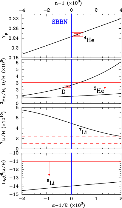
Figure 1: ⁴He mass fraction $Y_{\mathrm{p}}$ and number abundance ratios of D, ³He, ⁷Li and ⁶Li relative to H as a function of the power-law index of the scale factor $\alpha-1/2$ or the $f(R)$ function $n-1$. Solid curves show calculated results for the $f(R)\propto R^{n}$ model. The solid smaller and larger boxes of ⁴He and D abundances correspond to the $2\sigma$ and $4\sigma$ limits, respectively, from adopted observational constraints. The dashed box corresponds to the $2\sigma$ limits of ⁷Li abundance. The horizontal lines with downward arrows of ³He and ⁶Li abundances show observational upper limits. The result on the vertical line for $\alpha=1/2$ or $n=1$ is for the SBBN model. Note that the $f(R)$ function for $\alpha<1/2$ was corrected in this paper so that the cosmological model connects to the present $\Lambda$CDM model.

It is seen that the $2\sigma$ observational limits of ⁴He and D abundances are slightly inconsistent with the theoretical values for the SBBN, while their $4\sigma$ limits are consistent. In this figure, however, relatively small uncertainties coming from adopted nuclear reaction rates are not taken into account. Also, observational abundance determination may include some unknown systematic error. In addition, the disagreements of abundances are of the order of 10 % at most. The slight disagreements, therefore, do not seem so important at the moment, although they could be meaningful defects in the SBBN model in the future. In contrast to the disagreements, the ⁷Li abundance in the SBBN model is larger than observational limits by a factor of $\sim 3-4$. The SBBN values of ³He and ⁶Li abundances are, on the other hand, consistent with observational upper limits.

As proven in Sec. II, the cosmic expansion rate in the modified gravity model is increased when $\alpha$ increases. In particular, the expansion rate for $\alpha>1/2$ is always larger than in the SBBN model. All curves are understood as a result of a changed expansion rate as follows. First, when the expansion rate is larger, the freeze-out of weak reactions occurs earlier. The neutron abundance remaining after the freeze-out is then higher. Second, the time interval between the freeze-out and the ⁴He synthesis is shorter because of faster cosmic expansion. Neutron abundances are larger because of the above two reasons. Almost all neutrons are processed to form ⁴He nuclei at the ⁴He synthesis epoch. The ⁴He abundance is therefore larger for larger values of $\alpha$.

Because of the larger expansion rate, the reaction ¹H($n,\gamma$)²H also freezes out earlier. The relic neutron abundance right after the ⁴He synthesis then becomes higher. This higher neutron abundance significantly affects abundances of other light nuclei. D is predominantly produced via ¹H($n,\gamma$)²H. The higher neutron abundance then leads to higher D abundance. ³H is produced via ²H($d,p$)³H and destroyed via ³H($d,n$)⁴He. The enhanced D abundance leads to a higher ³H abundance by a higher production rate. ³He is produced via ²H($d,n$)³He and destroyed via ³He($n,p$)³H. The somewhat higher D abundance leads to a higher production rate, while the higher neutron abundance leads to a significantly higher destruction rate. Eventually, the ³He abundance is slightly higher. The primordial ³H abundance is the sum of ³H and ³He produced during the BBN. Long after the BBN, ³He nuclei $\beta$-decay into ³H nuclei. The final abundance of ³He is larger than that of ³H by about 2 orders of magnitude in SBBN. Therefore, the primordial ³H abundance predominantly reflects the larger ³He abundance during BBN.

⁷Li is produced via ⁴He($t,\gamma$)⁷Li and destroyed via ⁷Li($p,\alpha$)⁴He. The ⁷Li abundance is then higher because of the higher T abundance. ⁷Be is produced via ⁴He(³He$,\gamma$)⁷Be and destroyed via ⁷Be$(n,p$)⁷Li. A slightly higher abundance of ³He and a considerably higher abundance of the neutron leads to a smaller ⁷Be abundance. The primordial ⁷Li abundance is the sum of ⁷Li and ⁷Be produced during the BBN. Long after the BBN, ⁷Be nuclei recombine with electrons and are transformed to ⁷Li nuclei via the electron capture process. The abundance of ⁷Be is larger than that of ⁷Li in SBBN. Therefore, the larger expansion rate results in a smaller primordial ⁷Li abundance. ⁶Li is produced via ⁴He($d,\gamma$)⁶Li and destroyed via ⁶Li$(p,\alpha$)³He. The higher D abundance leads to a higher ⁶Li abundance.

We note that trends of theoretical curves in the modified gravity model are somewhat similar to those in the model including additional components of energy density, e.g., sterile neutrinos and a primordial magnetic field, within the framework of Einstein’s general relativity. A more illustrative and detailed explanation can be found for effects of the magnetic field on all light element abundances in Ref. Kawasaki:2012va .

When the $4\sigma$ limit of ⁴He is used, the constraints are derived,

$$-1\times 10^{-5}\lesssim \left(\alpha-1/2\right) \lesssim 5\times 10^{-4}$$

$$-2\times 10^{-5}\lesssim \left(n-1\right) \lesssim 10^{-3}.$$ (31)

When the $4\sigma$ limit of D is used, however, more stringent constraints are derived,

$$-3\times 10^{-4}\lesssim \left(\alpha-1/2\right) \lesssim 2\times 10^{-6}$$

$$-6\times 10^{-4}\lesssim \left(n-1\right) \lesssim 4\times 10^{-6}.$$ (32)

We find that the cases of $\alpha>1/2$ and $\alpha<1/2$ are constrained most stringently from the abundance constraints on D and ⁴He, respectively, for the following reasons. The $4\sigma$ range of D abundance is barely consistent with the SBBN result, and the upper limit is very close to the SBBN value. Since the D abundance increases with increasing $\alpha$ or $n$, the theoretical curve easily deviates from the observational limit for $\alpha>1/2$ (Fig. 1). On the other hand, the lower limit of ⁴He abundance is very close to the SBBN value. Since the ⁴He abundance also increases with increasing $\alpha$ or $n$, the theoretical curve easily deviates from the observational limit for $\alpha<1/2$.

Additionally, we find that the abundances of ³He and ⁶Li are not sensitive to the change of $\alpha$, and that they are within the adopted limits in the whole parameter region shown in Fig. 1. Although the ⁷Li abundance approaches the observed abundance level with increasing $\alpha$, it is always outside of the adopted limits in Fig. 1.

Figure 2 shows the likelihood function for the power-law index $\alpha-1/2$ or $n-1$ (solid curve). In this estimation, the likelihood function is defined as

$$L(\alpha)=L_{\mathrm{D}}(\alpha)L_{{}^{4}\mathrm{He}}(\alpha),$$ (33)

where the likelihood functions for respective nuclear abundances ($i=$D and ⁴He) are given by

$$L_{i}(\alpha)=\frac{1}{\sqrt{\mathstrut 2\pi}\sigma_{i,{\rm obs}}}\exp\left\{-\frac{\left[Y_{i,{\rm th}}(\alpha)-Y_{i,{\rm obs}}\right]^{2}}{2\sigma_{i,{\rm obs}}^{2}}\right\},$$ (34)

where $Y_{i,{\rm th}}(\alpha)$ is the theoretically calculated abundance of $i$, and $Y_{i,{\rm obs}}$ and $\sigma_{i,{\rm obs}}$ are the central value and 1 $\sigma$ error, respectively, of the adopted observational abundance of $i$. The solid curve has been normalized as $\int L(\alpha)d\alpha=1$.

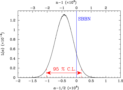
Figure 2: Likelihood function as a function of the power-law index $\alpha-1/2$ or $n-1$ (solid curve). This curve is estimated using the observational constraints on the D and ⁴He abundances. The parameter region bounded by vertical dashed lines is the 95 % C.L. The vertical solid line on $\alpha=1/2$ or $n=1$ corresponds to the SBBN model.

From the combination of the constraints on D and ⁴He abundances, we derive a 95 % C.L. on the parameters as

$$\left(\alpha-1/2\right) = \left(-0.43\pm 0.59\right)\times 10^{-4}$$

$$\left(n-1\right) = \left(-0.86\pm 1.19\right)\times 10^{-4}.$$ (35)

This parameter region is enclosed by vertical dashed lines. The solid vertical line corresponds to the SBBN model described by the general relativity ($\alpha=1/2$ or $n=1$). It is found that the deviation of the parameter $\alpha$ from $1/2$ is constrained to be less than ${\mathcal{O}}$($10^{-4}$). This constraint also indicates that even in the generalized model of the $f(R)$ gravity, the case of $n=1$ is very likely based upon the comparison of theoretical and observational nuclear abundances. If only the region of $\alpha>1/2$ is allowed, as in the case of the $f_{2}(R)$ function [Eq. (11)], the amplitude of $\alpha-1/2$ is constrained relatively strongly.

VI Summary

In this study we revisited effects of a modified gravity on BBN. The model is based on the $f(R)\propto R^{n}$ term in the action and the assumption of the scaling for the time evolution of scale factor $a(t)\propto t^{\alpha}$ in a homogeneous and isotropic universe. The $f(R)$ functions were constructed so that they describe the accelerated expansion of the present Universe successfully. We utilized a nuclear reaction network code and calculated all light element abundances in the modified gravity model. We compared the calculations with astronomical observations of primordial elemental abundances and found that the parameters are constrained to be $\left(\alpha-1/2\right)<{\mathcal{O}}(10^{-4})$ and $\left(n-1\right)<{\mathcal{O}}(10^{-4})$ mainly from the limits on primordial D and ⁴He abundances.

- (1) G. Lambiase and G. Scarpetta, Phys. Rev. D 74, 087504 (2006).
- (2) J. U. Kang and G. Panotopoulos, Phys. Lett. B 677, 6 (2009).
- (3) L. Kawano, NASA STI/Recon Technical Report N 92, 25163 (1992).
- (4) M. S. Smith, L. H. Kawano, and R. A. Malaney, Astrophys. J. Suppl. 85, 219 (1993).
- (5) R. H. Cyburt et al., Astrophys. J. Suppl. Ser. 189, 240 (2010).
- (6) K. A. Olive et al. (Particle Data Group Collaboration), Chin. Phys. C 38, 090001 (2014).
- (7) H. Ishida, M. Kusakabe, and H. Okada, Phys. Rev. D 90, 083519 (2014).
- (8) P. A. R. Ade et al. (Planck Collaboration), Astron. Astrophys. 571, A16 (2014).
- (9) Y. I. Izotov, T. X. Thuan, and N. G. Guseva, Mon. Not. Roy. Astron. Soc. 445, 778 (2014).
- (10) R. Cooke, M. Pettini, R. A. Jorgenson, M. T. Murphy, and C. C. Steidel, Astrophys. J. 781, 31 (2014).
- (11) T. M. Bania, R. T. Rood, and D. S. Balser, Nature 415, 54 (2002).
- (12) L. Sbordone et al., Astron. Astrophys. 522, A26 (2010).
- (13) K. Lind, J. Melendez, M. Asplund, R. Collet, and Z. Magic, Astron. Astrophys. 544, A96 (2013).
- (14) M. Kawasaki and M. Kusakabe, Phys. Rev. D 86, 063003 (2012).