Interrupted Stellar Encounters in Star Clusters

Abstract

Strong encounters between single stars and binaries play a pivotal role in the evolution of star clusters. Such encounters can also dramatically modify the orbital parameters of binaries, exchange partners in and out of binaries, and are a primary contributor to the rate of physical stellar collisions in star clusters. Often, these encounters are studied under the approximation that they happen quickly enough and within a small enough volume to be considered isolated from the rest of the cluster. In this paper, we study the validity of this assumption through the analysis of a large grid of single – binary and binary – binary scattering experiments. For each encounter we evaluate the encounter duration, and compare this with the expected time until another single or binary star will join the encounter. We find that for lower-mass clusters, similar to typical open clusters in our Galaxy, the percent of encounters that will be “interrupted” by an interloping star or binary may be 20-40% (or higher) in the core, though for typical globular clusters we expect $\lesssim$1% of encounters to be interrupted. Thus, the assumption that strong encounters occur in relative isolation breaks down for certain clusters. Instead, many strong encounters develop into more complex “mini-clusters”, which must be accounted for in studying, for example, the internal dynamics of star clusters, and the physical stellar collision rate.

1. Introduction

The evolution of (collisional) star clusters is often conceptualized, at a basic level, as being governed by the combination of the long-range cumulative effects of weak stellar encounters, known as “two-body relaxation”, and the results of short-range strong stellar encounters between individual stars and binaries. In Monte Carlo models for globular cluster (GC) evolution, this assumption is more than a conceptual convenience, and is inherent to the functionality of the code (e.g. Spurzem & Giersz, 1996; Joshi et al., 2000; Vasiliev, 2015). Two-body relaxation allows stars to gradually exchange energy, which evolves the cluster towards thermal equilibrium, and drives the processes of evaporation, mass segregation and core collapse. It has long been known that close encounters with “hard” binaries (i.e., those with relatively large binding energy compared to the kinetic energies of cluster stars, Heggie 1975) can halt core collapse by donating energy to other stars in the encounter, which can be given back to the cluster through two-body relaxation processes. This type of strong encounter may decrease the semi-major axis of the binary, and indeed, strong encounters can modify all orbital parameters of binaries, exchange stars into and out of binaries, and even result in physical stellar collisions. Moreover, strong encounters are a key component to star cluster evolution (Hut, 1983), and they can alter a binary population from its characteristics at birth (e.g. Ivanova et al., 2005; Hurley et al., 2007; Marks et al., 2011; Geller et al., 2013a, b, 2015; Leigh & Geller, 2015).

As such, the outcomes of single – binary (1+2) and binary – binary (2+2) encounters are well studied (e.g. Heggie, 1975; Hills, 1975; Hut & Bahcall, 1983; Fregeau et al., 2004), and more recently stellar encounters involving triples are also gaining importance (Leigh & Geller, 2012, 2013). Apart from direct $N$-body star cluster simulations (Aarseth, 2003; Wang et al., 2015), it is typical to make the simplifying assumption that such encounters happen rapidly enough, and within a small enough volume, that they are effectively isolated from the rest of the cluster. With such assumptions, one can run many few-body scattering experiments, each involving perhaps 3-6 stars, to derive statistical cross sections of the outcomes of such encounters (e.g. Hut & Bahcall, 1983; Fregeau et al., 2004), and apply this knowledge to help understand the more complex evolution of a full star cluster, which itself may contain many hundreds to millions of stars.

In this paper we investigate the validity of the assumption of treating these strong encounters as isolated. In reality the encounters occur within a star cluster, and most often in the dense cluster core, where they may not be allowed to progress fully on their own. More specifically, we use the numerical scattering code FEWBODY (Fregeau et al., 2004), to perform millions of isolated 1+2 and 2+2 scattering experiments, described in Section 2. We then compare the total encounter duration to the predicted time until another single or binary star would join, or “interrupt”, this ongoing stellar encounter, as defined in Section 3. We find that for certain cluster parameters, the fraction of interrupted strong encounters can reach over 40% (Section 4). Finally in Sections 5 and 6 we discuss the implications of these findings and provide our conclusions.

2. $N$-body Scattering Simulations

We present results from $>10^{7}$ individual 1+2 and 2+2 numerical scattering experiments performed using the FEWBODY code (Fregeau et al., 2004). We choose parameters for these scattering experiments that are relevant for the cores of star clusters with total masses ($M_{\text{cl}}$) and half-mass radii ($R_{\text{hm}}$) covering the range of observed open clusters (OCs) and GCs in our Galaxy. Specifically, we sample a grid in $M_{\text{cl}}$ extending from $10^{2}$ to $10^{6}$ M_⊙ in steps of 0.5 in $\log_{10}(M_{\text{cl}}$ [M_⊙] $)$, and in $R_{\text{hm}}$ from 1 to 10 pc in steps of 1 pc. We performed two sets of experiments over this grid, one drawing from a mass function appropriate for an old GC, at an age of 10 Gyr and $\text{[Fe/H]}=-1.5$, and the other drawing from a mass function more appropriate for an OC, at an age of 300 Myr and $\text{[Fe/H]}=0$.

For a single star in a given scattering experiment, we choose a stellar mass from a Kroupa et al. (1993) initial mass function (IMF) between 0.1 M_⊙ and the turnoff mass at the age of the cluster ($\sim$0.95 M_⊙ at 10 Gyr and $\text{[Fe/H]}=-1.5$, and $\sim$2.96 M_⊙ at 300 Myr and $\text{[Fe/H]}=0$). For a binary, we first choose the primary mass ($m_{1}$) from the same mass function and within the same mass limits. We then draw a mass ratio ($q=m_{2}/m_{1}$) from a uniform distribution to select the secondary mass ($m_{2}$), and enforce the criteria that $q\leq 1$ and $m_{2}>0.1$ M_⊙. We derive a radius for each star using this stellar mass and the cluster [Fe/H], following the method of Tout et al. (1996), which we provide to FEWBODY for identifying physical collisions during the encounters (see Fregeau et al. 2004 and Leigh & Geller 2012 for more details).

We choose binary orbital elements from the observed distributions of binaries with solar-type primary stars in the Galactic field from Raghavan et al. (2010), which are also consistent with observations of solar-type binaries in OCs (e.g., Geller et al., 2010, 2013a; Geller & Mathieu, 2012). Specifically, we draw orbital periods from a log-normal distribution (with a mean of $\log(P$ [days]) = 5.03 and $\sigma$ = 2.28), with a short period limit at the Roche radius (Eggleton, 1983) and a long-period limit at the “hard-soft boundary” of the core. Thus we require detached hard binaries initially, and assume that soft binaries are disrupted promptly and are generally not as relevant for the dynamical evolution of the cluster. We estimate the maximum period for a given hard binary, $P_{\text{hs}}$, using the virial theorem, such that,

$$P_{\text{hs}}=\frac{\pi G}{\sqrt{2}}\left(\frac{m_{1}m_{2}}{m_{3}}\right)^{3/2}\left(m_{1}+m_{2}\right)^{-1/2}\sigma_{0}^{-3},$$ (1)

where $m_{3}$ is the mass of the incoming object (either a single star or the combined mass of a binary), and $\sigma_{0}$ is the three-dimensional velocity dispersion (assumed to be $\sigma_{0}=\sqrt{3}\sigma_{\text{0,1D}}$). As we discuss in Section 5, we ran additional experiments drawing binary orbital periods from a uniform distribution in $\log(P)$, a common theoretical assumption. Finally, we draw eccentricities from a uniform distribution, and choose all angles of the encounter randomly.

For the majority of our experiments, we choose the impact parameter for a given encounter randomly from a uniform distribution between 0 and 1 times the binary semi-major axis in a 1+2 encounter, or the sum of the two binary semi-major axes for a 2+2 encounter. We discuss additional experiments with larger impact parameters in Section 5. The velocity at infinity for the incoming object is drawn from a lowered Maxwellian distribution (typical for star clusters), which is defined by the velocity dispersion and the escape velocity, both calculated at the center of a Plummer (1911) model (with the given $M_{\text{cl}}$ and $R_{\text{hm}}$).

The above parameters define discrete 1+2 and 2+2 scattering experiments that are appropriate for the cores of typical Milky Way star clusters. For each of our 90 clusters, we perform $10^{4}$ 1+2 and the equivalent number of 2+2 unique numerical scattering experiments (at two different cluster ages and two different period distributions, as well as a subset at higher impact parameters). We discuss results from these $>10^{7}$ scattering experiments in the following sections.

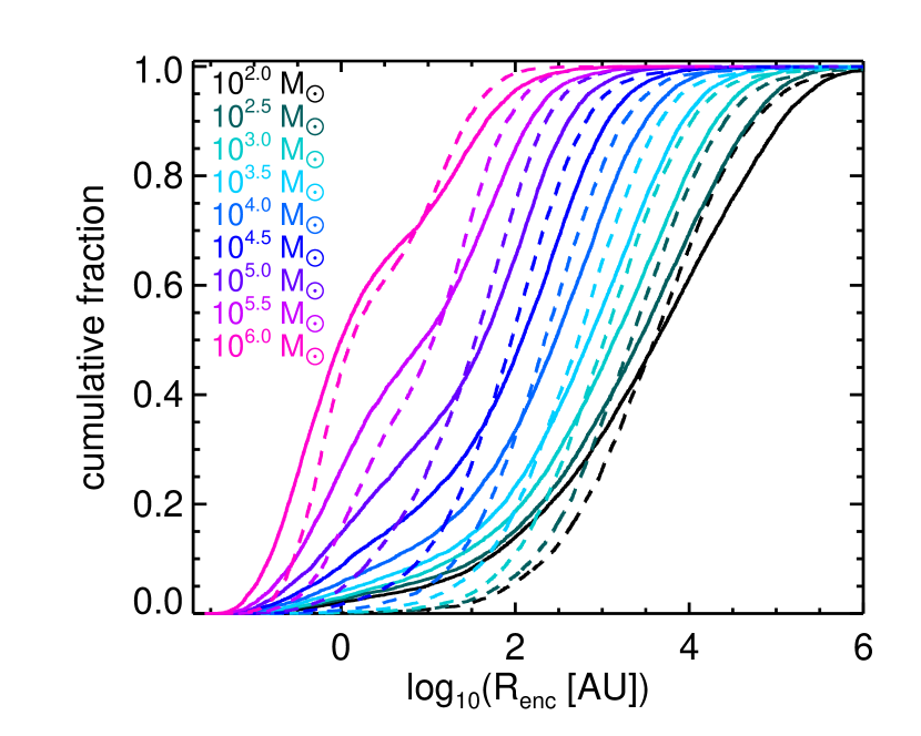
Figure 1.— Cumulative distributions of the mean sizes ($R_{\text{enc}}$) of 1+2 (solid lines) and 2+2 (dashed lines) encounters drawn from clusters with $R_{\text{hm}}=3$pc, over all $M_{\text{cl}}$ in our grid (as annotated in the figure), and using the 10 Gyr mass function.

3. Encounter Timescales

There are two relevant timescales for the purposes of this study. The first is the encounter duration, which we will call $t_{\text{d}}$. The second is the time until another single or binary star will join, or “interrupt”, this ongoing 1+2 or 2+2 encounter, which we will call $t_{\text{e}}$. The first timescale, $t_{\text{d}}$, is calculated and outputted by FEWBODY; we refer the reader to Fregeau et al. (2004), and specifically Sections 3.3.4 and 3.3.5 and Equations 5 and 6, for details. In short, FEWBODY uses stability assessment techniques along with a few simple rules to determine when the separate components of the encounter (including stable hierarchies) will no longer interact with each other or evolve internally, at which point the encounter is deemed complete. These criteria depend on a tolerance parameter $\delta=F_{\text{tid}}/F_{\text{rel}}$, the ratio of the tidal-to-binding (i.e., relative) forces at apocenter, which we set to the FEWBODY default value of $\delta=10^{-5}$. (In general, smaller values of $\delta$ yield more accurate results.) As we discuss in Section 5, our results are only minimally sensitive to changes in $\delta$.

To calculate the second timescale, $t_{\text{e}}$, we must first find the time for a single (₁) or binary (₂) star to interrupt an ongoing 1+2 (₃) or 2+2 (₄) encounter, which we will refer to as, respectively, $\tau_{3+1}$, $\tau_{3+2}$, $\tau_{4+1}$, and $\tau_{4+2}$. We define these timescales as follows.

$$\beta =\left(\frac{10^{3}\text{ pc}^{-3}}{n_{0}}\right)\left(\frac{v_{\text{rms,0}}}{5\text{ km s}^{-1}}\right)\left(\frac{0.5\text{ M}_{\odot}}{\langle m\rangle}\right)\left(\frac{1\text{ AU}}{R_{\text{enc}}}\right)\text{ ,}$$

$$\tau_{3+1} =5.4\times 10^{10}\left(1-f_{\text{b}}\right)^{-1}\beta\text{ yr ,}$$

$$\tau_{4+1} =4.2\times 10^{10}\left(1-f_{\text{b}}\right)^{-1}\beta\text{ yr ,}$$

$$\tau_{3+2} =4.2\times 10^{10}f_{\text{b}}^{-1}\beta\text{ yr ,}$$

$$\tau_{4+2} =1.8\times 10^{10}f_{\text{b}}^{-1}\beta\text{ yr ,}$$

where $n_{0}$ is the central number density, $v_{\text{rms,0}}$ is the central root-mean-square velocity (and we assume $v_{\text{rms,0}}=\sigma_{0}=\sqrt{3}\sigma_{\text{0,1D}}$), $\langle m\rangle$ is the mean mass of a star in the cluster, $R_{\text{enc}}$ is the mean radius of the encounter, (e.g., used to calculate the encounter’s mean geometric cross-section, $\pi$$R_{\text{enc}}^{2}$, see also Figure 1), and $f_{\text{b}}$ is the binary frequency. We derive these equations following the procedure in Leonard (1989), with numerical pre-factors derived following Leigh & Sills (2011). Finally, the time until a subsequent encounter is given by,

$$t_{\text{e}}=\begin{cases}\left(\Gamma_{3+1}+\Gamma_{3+2}\right)^{-1}&\text{, for 1+2}\\ \left(\Gamma_{4+1}+\Gamma_{4+2}\right)^{-1}&\text{, for 2+2},\\ \end{cases}$$ (3)

where $\Gamma=1/\tau$.

Most of the parameters in Equation 3 come directly from the input values discussed above, and the assumption of a Plummer model for the cluster. We describe our calculation of the remaining parameters below.

To calculate $n_{0}$ from the Plummer model, we first estimate the total number of stars by randomly drawing sufficient single stars from the appropriate mass function (discussed above), to reach the cluster mass, $M_{\text{cl}}$. In order to reduce stochastic effects, we perform this estimate multiple times, until the standard error on the mean number of stars derived for the cluster is $<0.01M_{\text{cl}}$.

We modified FEWBODY to calculate and output the mean of the maximum separation between any two stars in the encounter at every time step, and divide this value by two to get $R_{\text{enc}}$. At a given $R_{\text{hm}}$, the $R_{\text{enc}}$ distribution shifts toward lower values with larger $M_{\text{cl}}$ (see Figure 1). This is primarily due to the dependence of the hard-soft boundary on $M_{\text{cl}}$ (through $\sigma_{0}$), which shifts the distributions of binary semi-major axes, and also (by definition) the impact parameters, towards smaller values at larger $M_{\text{cl}}$.

Finally, to estimate the binary frequency, $f_{\text{b}}$, for a cluster with a given $M_{\text{cl}}$ and $R_{\text{hm}}$, we first estimate the expected average hard-soft boundary in the core of the cluster, as the mean of the $P_{\text{hs}}$ values (from Equation 1) for each encounter. We then calculate the fraction of the log-normal input period distribution below this hard-soft boundary, $f_{P}$, and assume that, if the full period distribution could be occupied, this would result in a 50% binary frequency (Raghavan et al., 2010). To find the (hard) binary frequency for the cluster, we simply multiply $f_{\text{b}}=0.5f_{P}$. In this way, we assume the total number of objects (binaries plus singles) in the cluster is fixed. The resulting $f_{\text{b}}$ values decrease toward higher $M_{\text{cl}}$ and lower $R_{\text{hm}}$ (Figure 2), as is consistent with observed star clusters (e.g., Leigh et al., 2015).

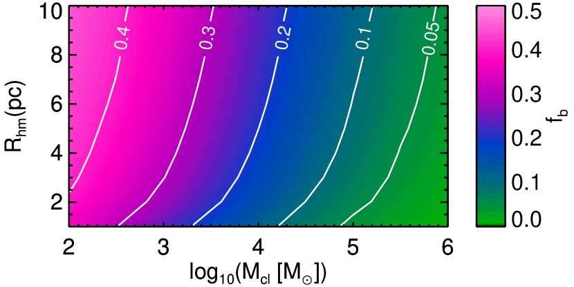
Figure 2.— Contour plot of the binary frequencies ($f_{\text{b}}$) that result from our estimates of the hard-soft boundary, a field binary frequency of 50%, and the 10 Gyr mass functions, for the given $R_{\text{hm}}$ and $M_{\text{cl}}$ values, as discussed in Section 2. (The colors and lines show the same values.)

4. Fraction of Interrupted Stellar Encounters

We find from these scattering experiments that the percent of ongoing stellar encounters that are expected to be interrupted by an interloping single or binary star in a star cluster core ranges from below 1% to over 40%. The main results are plotted in Figures 3 and 4.

For both the 1+2 and 2+2 experiments, we find that $t_{\text{e}}$ is only minimally sensitive to the cluster mass (Figure 3). Though the encounter’s geometric cross-section ($\pi$$R_{\text{enc}}^{2}$), and binary frequency, both decrease with increasing cluster mass (see Figures 1 and 2), the increase in central density roughly cancels out this effect. On the other hand, the distribution of $t_{\text{d}}$ changes dramatically with cluster mass, shifting toward shorter encounter durations and developing a pronounced bimodal shape at higher $M_{\text{cl}}$.

The shift toward shorter encounter durations at higher $M_{\text{cl}}$ is due to the corresponding decrease in the semi-major axis at the hard-soft boundary, which results in tighter binaries involved in the encounters. The encounter duration is then shorter due to the characteristically lower total angular momentum.

The emerging bimodal structure in the distribution of $t_{\text{d}}$ at higher $M_{\text{cl}}$ arises from an increasing frequency of physical collisions. Indeed the fraction of encounters that result in a physical stellar collision in the cores of our most massive and centrally concentrated clusters reaches nearly 90% (due to the more compact binaries involved in the encounters). In the diagonally hatched histograms in Figure 3, we highlight the subset of encounters that end with $\leq 2$ stars remaining (due to collisions) which clearly dominate the peaks at short $t_{\text{d}}$. With only two (or in some cases one) stars remaining, an encounter is considered to be finished, by definition, and therefore on average will not last as long as a similar resonant encounter that does not result in a physical collision.

In Figure 4, we compare $t_{\text{d}}$ and $t_{\text{e}}$ for each individual encounter directly (rather than as an ensemble). In the core of a typical GC, at $M_{\text{cl}}\sim 10^{5.5}$ M_⊙ and $R_{\text{hm}}\sim 3$ pc, $\lesssim$1% of encounters are expected to be interrupted. However, in the cores of typical OCs, at $M_{\text{cl}}\leq 10^{3}$ M_⊙ and $R_{\text{hm}}\leq 3$ pc, the fraction of ongoing encounters that are expected to be interrupted by an incoming single or binary star is $\gtrsim 25$%, and reaches $>40$% for the lowest mass and most compact clusters.

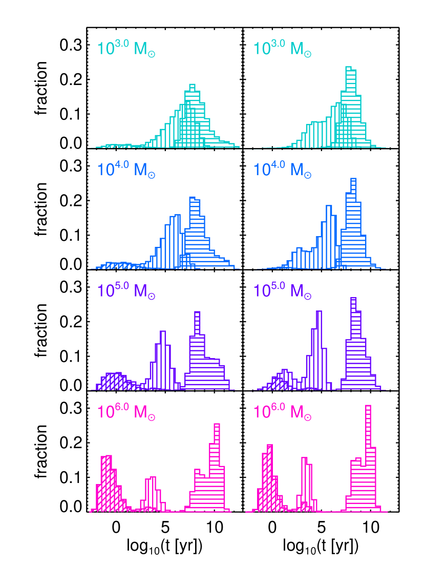
Figure 3.— Distributions of the total encounter durations ($t_{\text{d}}$; vertically hatched histograms) and times until the next encounter ($t_{\text{e}}$; horizontally hatched histograms) for the 1+2 (left panel) and 2+2 (right panel) scattering experiments drawn from clusters with $R_{\text{hm}}=3$pc and the $M_{\text{cl}}$ values indicated in each panel, for the 10 Gyr mass function. The diagonally hatched histograms show the encounters that resulted in at least 1 (left panel) or 2 (right panel) physical stellar collision(s). All histograms are normalized by the total number of encounters.

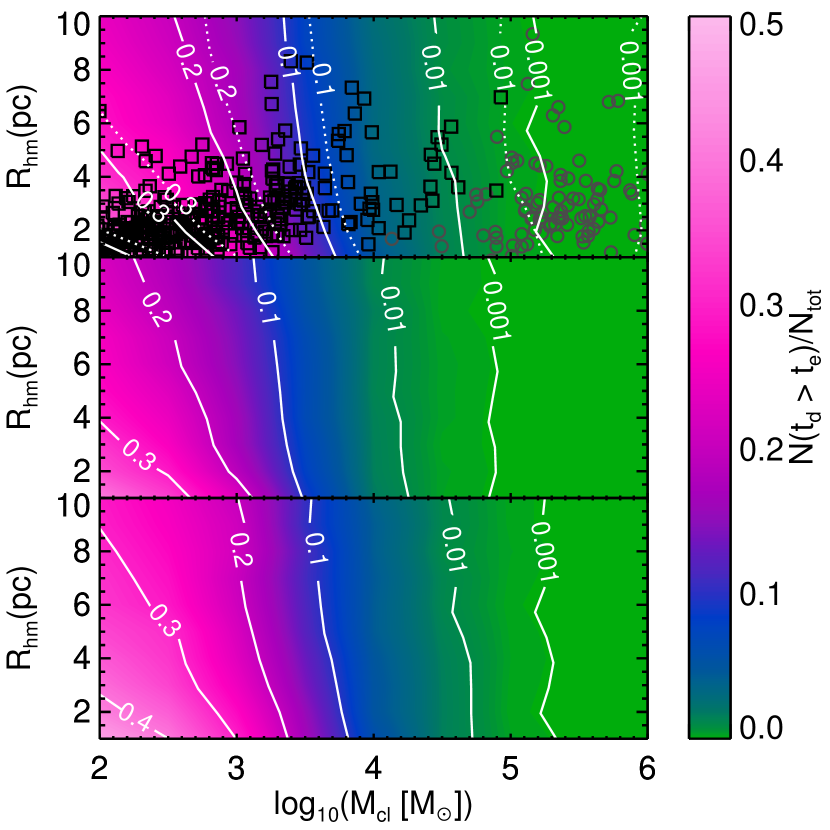
Figure 4.— Contour plots showing the fraction of interrupted encounters (where the encounter duration is greater than the predicted time until the next encounter: $t_{\text{d}}>t_{\text{e}}$, see Equation 3) for clusters with the given total masses, $M_{\text{cl}}$, and half-mass radii, $R_{\text{hm}}$. The top panel shows the average fraction from all encounters, weighted by the 1+2 and 2+2 encounter timescales from Leigh & Sills (2011). The bottom and middle panels shows the separate results for our 1+2 and 2+2 scattering experiments, respectively. The color shading and solid lines show (the same) results for the 10 Gyr (and sub-solar metallicity) mass function. In the top panel we also show results for the 300 Myr (and solar metallicity) mass function with the dotted lines. For reference we also plot a sample of observed GCs (Harris, 1996) with the gray circles, and OCs (Piskunov et al., 2008; Kharchenko et al., 2013) with the black squares. (Note, for the OCs, we estimate $R_{\text{hm}}$ from the King core and tidal radii from Kharchenko et al. 2013).

5. Discussion

We find that a substantial fraction of strong encounters may be interrupted, while they are ongoing, by an interloping single or binary star in the cluster. In this case, the common assumption of encounters progressing fully in isolation breaks down, and instead the encounter develops into a “mini-cluster” with a more complicated dynamical evolution. The fraction of interrupted encounters is largest for OCs (see Figure 4), where, on average, the encounter geometric cross-sections are the largest (Figure 1) and the encounter durations are the longest (Figure 3). For numerical models of star clusters, this result is encouraging, as OCs are most often modeled with direct $N$-body methods (e.g., Aarseth, 2003), which naturally account for stars or binaries interrupting an ongoing encounter. GCs are more often modeled with Monte Carlo codes (e.g., Chatterjee et al., 2010; Hypki & Giersz, 2013), where stellar encounters are assumed to run to completion in isolation, though direct $N$-body models are now approaching realistic GCs (Wang et al., 2015). Fortunately, as Figure 4 indicates, this assumption is much more valid (albeit not perfect) in massive GCs.

In the following, we briefly discuss a few additional processes and parameters that may increase or decrease the fraction of interrupted encounters, though all of which only contribute factors of approximately order unity.

First, we did not account for any effects of two-body relaxation, which leads to mass segregation and the preferential loss of lower-mass single stars from the cluster, and thereby tends to increase $\langle m\rangle$ and $f_{\text{b}}$ (e.g., Geller et al., 2013a). Increasing $\langle m\rangle$ decreases $t_{\text{e}}$, and therefore tends to increase the fraction of interrupted encounters. Increasing $f_{\text{b}}$ gives more weight to the 2+2 encounters in our calculations, and may increase or decrease the overall fraction of interrupted encounters accordingly.

Second, just as stars can be tidally stripped from a star cluster by the Galactic potential, stars involved in a strong encounter may endure an analogous process owing to the cluster potential. Following this analogy, we estimate an effective tidal radius for each encounter,

$$r_{\text{t,eff}}=\left(\frac{M_{\text{enc}}}{M_{\text{core}}}\right)^{1/3}r_{\text{core}}\text{ ,}$$ (4)

where $M_{\text{enc}}$ is the total stellar mass of the encounter, $M_{\text{core}}$ is the core mass of the star cluster, $r_{\text{core}}$ is the core radius of the cluster, and we assume that the encounter occurs at $\lesssim 1r_{\text{core}}$ from the cluster center. (Here, we estimate both $M_{\text{core}}$ and $r_{\text{core}}$ from the Plummer model.) If we assume that any encounter with, $R_{\text{enc}}>r_{\text{t,eff}}$ would be tidally disrupted before it is interrupted, this decreases the fraction of interrupted encounters by $\sim$15% (almost independent of $M_{\text{cl}}$ and $R_{\text{hm}}$).

We ran additional scattering experiments drawing binary orbital periods from a uniform distribution in $\log(P)$, within the same period limits as for the log-normal period distribution. For the same cluster parameters, this decreases the fraction of interrupted encounters by a factor of $\sim$2 over nearly all $M_{\text{cl}}$ and $R_{\text{hm}}$, owing to the larger fraction of short-period binaries (with smaller geometric cross sections) as compared to the more empirically motivated log-normal period distribution.

Additionally, we ran scattering experiments drawing impact parameters from uniform distributions extending from zero to 5, 10, 15 and 20 times the size of the binary, respectively, and find nearly no change in the fraction of interrupted encounters from the results presented above.

We also ran scattering experiments with $\delta$ values of $10^{-7}$, $10^{-6}$, $10^{-5}$, $10^{-4}$, and $10^{-3}$, respectively. We find that the fraction of interrupted encounters decreases slightly with smaller $\delta$ (i.e., more accurate outcome classifications in FEWBODY), and asymptotes at small $\delta$ toward a value of $\sim 0.7$ times the results at our default $\delta=10^{-5}$.

In closing, one important implication of our results may be to increase the expected rate of physical stellar collisions between two (or more) stars in star clusters. In previous papers, we showed that, for fixed total energy and angular momentum, the probability of a physical collision during a stellar encounter increases as the number of stars in the encounter increases (Leigh & Geller, 2012, 2015). Thus if additional stars join an ongoing encounter, this should increase the probability of a collision. Moreover, collision rates (or cross sections) calculated from isolated scattering experiments may only be lower limits on the true collision rates in star clusters.

6. Conclusions

Strong stellar encounters in star clusters do not always run to completion without another stellar interloper cutting in on the gravitational dance. Indeed, we find that $\sim 20-40$% of encounters in the cores of OCs may be interrupted before completion (see Figure 4). Moreover, our results suggest that an assumption of isolated encounters is frequently invalid in the OC regime, and instead many encounters may develop into small-$N$ “mini-clusters”, though this assumption may still be valid in more massive GCs. Finally, the probability of a physical stellar collision increases with an increasing number of stars in an encounter (e.g. Leigh & Geller, 2015), and therefore these interrupted encounters may enhance the rate of stellar collisions in star clusters relative to what is assumed from isolated encounters alone.

References

- Aarseth (2003) Aarseth, S. J. 2003, Gravitational N-Body Simulations (Cambridge, UK: Cambridge University Press)
- Chatterjee et al. (2010) Chatterjee, S., Fregeau, J. M., Umbreit, S., & Rasio, F. A. 2010, ApJ, 719, 915
- Eggleton (1983) Eggleton, P. P. 1983, ApJ, 268, 368
- Fregeau et al. (2004) Fregeau, J. M., Cheung, P., Portegies Zwart, S. F., & Rasio, F. A. 2004, MNRAS, 352, 1
- Geller et al. (2013b) Geller, A. M., de Grijs, R., Li, C., & Hurley, J. R. 2013b, ApJ, 779, 30
- Geller et al. (2015) Geller, A. M., de Grijs, R., Li, C., & Hurley, J. R. 2015, ApJ, 805, 11
- Geller et al. (2013a) Geller, A. M., Hurley, J. R., & Mathieu, R. D. 2013a, AJ, 145, 8
- Geller & Mathieu (2012) Geller, A. M., & Mathieu, R. D. 2012, AJ, 144, 54
- Geller et al. (2010) Geller, A. M., et al. 2010, AJ, 139, 1383
- Harris (1996) Harris, W. E. 1996, AJ, 112, 1487
- Heggie (1975) Heggie, D. C. 1975, MNRAS, 173, 729
- Hills (1975) Hills, J. G. 1975, AJ, 80, 809
- Hurley et al. (2007) Hurley, J. R., Aarseth, S. J., & Shara, M. M. 2007, ApJ, 665, 707
- Hut (1983) Hut, P. 1983, ApJ, 272, L29
- Hut & Bahcall (1983) Hut, P., & Bahcall, J. N. 1983, ApJ, 268, 319
- Hypki & Giersz (2013) Hypki, A., & Giersz, M. 2013, MNRAS, 429, 1221
- Ivanova et al. (2005) Ivanova, N., Belczynski, K., Fregeau, J. M., & Rasio, F. A. 2005, MNRAS, 358, 572
- Joshi et al. (2000) Joshi, K. J., Rasio, F. A., & Portegies Zwart, S. 2000, ApJ, 540, 969
- Kharchenko et al. (2013) Kharchenko, N. V., et al. 2013, A&A, 558, A53
- Kroupa et al. (1993) Kroupa, P., Tout, C. A., & Gilmore, G. 1993, MNRAS, 262, 545
- Küpper et al. (2010) Küpper, A. H. W., Kroupa, P., Baumgardt, H., & Heggie, D. C. 2010, MNRAS, 407, 2241
- Leigh & Geller (2012) Leigh, N., & Geller, A. M. 2012, MNRAS, 425, 2369
- Leigh & Sills (2011) Leigh, N., & Sills, A. 2011, MNRAS, 410, 2370
- Leigh & Geller (2013) Leigh, N. W. C., & Geller, A. M. 2013, MNRAS, 432, 2474
- Leigh & Geller (2015) Leigh, N. W. C., & Geller, A. M. 2015, MNRAS, 450, 1724
- Leigh et al. (2015) Leigh, N. W. C., et al. 2015, MNRAS, 446, 226
- Leonard (1989) Leonard, P. J. T. 1989, AJ, 98, 217
- Marks et al. (2011) Marks, M., Kroupa, P., & Oh, S. 2011, MNRAS, 417, 1684
- Piskunov et al. (2008) Piskunov, A. E., et al. 2008, A&A, 477, 165
- Plummer (1911) Plummer, H. C. 1911, MNRAS, 71, 460
- Raghavan et al. (2010) Raghavan, D., et al. 2010, ApJS, 190, 1
- Spurzem & Giersz (1996) Spurzem, R., & Giersz, M. 1996, MNRAS, 283, 805
- Tout et al. (1996) Tout, C. A., Pols, O. R., Eggleton, P. P., & Han, Z. 1996, MNRAS, 281, 257
- Vasiliev (2015) Vasiliev, E. 2015, MNRAS, 446, 3150
- Wang et al. (2015) Wang, L., et al. 2015, MNRAS, 450, 4070
- Webb et al. (2013) Webb, J. J., Harris, W. E., Sills, A., & Hurley, J. R. 2013, ApJ, 764, 124