Non-perturbative renormalization group calculation of the quasi-particle
velocity and the dielectric function of graphene
Carsten Bauer, Andreas Rückriegel, Anand Sharma, and
Peter Kopietz
Institut für Theoretische Physik, Universität Frankfurt, Max-von-Laue Strasse 1, 60438 Frankfurt, Germany
(June 29, 2015)
Abstract
Using a non-perturbative functional renormalization group
approach we calculate the renormalized
quasi-particle velocity and the
static dielectric function of suspended graphene as functions
of an external momentum .
Our numerical result for can be fitted by
,
where is the bare Fermi velocity, is an ultraviolet cutoff, and
,
for the physically relevant value () of the coupling constant.
In contrast to calculations based on the static random-phase approximation, we find that
approaches unity for .
Our result for agrees very well with a recent measurement
by Elias et al. [Nat. Phys. 7, 701 (2011)].
pacs:
81.05.ue, 11.10.Hi, 71.10.-w
At low energies the physical properties of graphene are dominated by
the Dirac points where the energy dispersion vanishes linearly.
In this regime many-body effects become important and can be measured
experimentally Kotov12 .
In view of the great interest in graphene both for fundamental research and applied physics,
it is important to gain a thorough understanding of correlation effects.
Of particular interest is the renormalization of the Fermi velocity
at the Dirac points by long-range Coulomb interactions, which
has been observed experimentally in suspended graphene using cyclotron resonance Elias11 , in ARPES measurements of quasi-freestanding graphene on SiC Siegel11 , and in graphene on hexagonal boron nitride (hBN) Yu13 .
Early one-loop renormalization group (RG) calculations Gonzalez94
predicted a logarithmic enhancement of the renormalized
Fermi velocity,
(1)
where is the infrared cutoff introduced in the RG procedure,
is an ultraviolet cutoff of the order of the inverse lattice spacing,
is the bare Fermi velocity,
and is the relevant dimensionless coupling constant.
Because for graphene suspended in vacuum
is rather large, perturbative RG calculations are not
expected to be quantitatively accurate.
In this work, we use a functional renormalization group
(FRG) approach Kopietz10 ; Metzner12
to derive non-perturbative RG flow equations for the cutoff- and momentum-dependent
velocity and the static dielectric
function of suspended graphene.
Since we are interested in
the RG flow of momentum-dependent functions,
the field theoretical RG is not sufficient, because with this method
one can only keep track of a
finite set of coupling constants.
We show here that this problem
can be solved within the FRG formalism Kopietz10 ; Metzner12 ;
specifically, we derive two coupled integro-differential
equations for the cutoff-dependent functions
and which are
non-perturbative in and self-consistently
describe the interplay between self-energy
and screening effects.
Our starting point is the following effective Hamiltonian describing
the low-energy physics of graphene,
(2)
where labels the two Dirac points
of the underlying tight-binding model on a honeycomb lattice,
is the bare Fermi velocity at Dirac point ,
and are two-component fermionic field operators
whose components are associated with the two
sublattices of the honeycomb lattice.
The two-component vector
contains Pauli matrices
acting on sublattice space, and
two-dimensional momentum integrations are denoted by
.
The interaction in Eq. (2)
is specified in terms of
the Fourier transform
of the Coulomb interaction and the Fourier components
of the density operators, .
For simplicity, we
consider a given spin projection and
suppress the spin label. We shall insert the spin-degeneracy
of the electrons in Eq. (10) below.
To derive FRG flow equations, we introduce a cutoff which inhibits
the propagation of electrons with momenta .
For our purpose it is sufficient
to work with a sharp momentum cutoff.
The regularized free propagator is then
,
where the label represents momentum
and fermionic Matsubara frequency .
At some large initial cutoff of the order of the inverse lattice spacing the regularized
Euclidean action of our system is
(3)
where is a two-component Grassmann field
and we have used a Hubbard-Stratonovich transformation
to represent the Coulomb interaction in terms of a scalar field
which couples to the Fourier components
of the density.
The integration symbols are and
.
Here
, where is a bosonic
Matsubara frequency.
It is now straightforward to write down a formally exact
flow equation for the generating functional
of the irreducible vertices describing their change
as we reduce the infrared cutoff . By construction
for the flowing vertices reduce to the exact
irreducible vertices of our original
Hamiltonian (2). As usual, we obtain an approximate
solution of this functional flow equation
by working with a truncated form of .
For our purpose, the following truncation is sufficient,
(4)
where in the last term
is the sublattice label
and , are the sublattice components of and the adjoint spinor .
It is convenient to express the renormalized fermionic and bosonic
propagators in terms of the corresponding self-energies as usual,
and
.
Note that the fermionic self-energy is a matrix in the sublattice labels.
Our truncation (4) retains only those vertices which
are already present in the bare action (3).
Although higher order vertices with more than
three external legs are generated by the RG procedure, they are irrelevant
at the Gaussian fixed point. In fact, a simple scaling analysis
keeping the Gaussian part of invariant
shows that the renormalized vertices with external legs
scale as , implying that all vertices
with external legs are irrelevant.
There are five marginal vertices
with three external legs, corresponding to the field combinations
,
,
,
, and .
While in our cutoff scheme
the purely bosonic -vertex
does not couple to the flow of the self-energies
and ,
the sublattice-changing vertices
of the type and
are neglected in Eq. (4).
We nevertheless believe that our truncation
(4) is accurate because the sublattice-preserving vertices of the type
and
are already finite in the bare action
(3).
Within our truncation and cutoff scheme, the self-energies
and three-legged vertices appearing in Eq. (4)
satisfy the following system of FRG flow equations,
(5a)
(5b)
(5c)
where for simplicity we have omitted the cutoff label and
the single-scale propagator is
(6)
The derivation of the above FRG equations starting from the general
Wetterich equation Wetterich93 for the
theory defined in Eq. (3)
is similar to the derivation
of the vertex expansion for mixed Bose-Fermi models discussed in
Refs. [Schuetz05, ; Kopietz10, ].
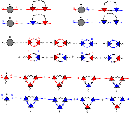
A graphical representation of the flow
equations (5a–5c)
is shown in Fig. 1.
Figure 1: (Color online)
Diagrammatic repesentation of the FRG flow equations
(5a–5c) for the fermionic self-energy
(first two lines), for the polarization (third and fourth line), and
the three-legged vertices (last two lines).
Solid arrows represent the exact cutoff-dependent
fermionic propagators,
wavy lines represent the corresponding bosonic propagators, and single-scale propagators
have an additional slash.
The dot over the vertices on the left-hand side represents
the derivative with respect to the cutoff .
The shaded triangles represent renormalized three-legged vertices with one bosonic and
two fermionic external legs carrying the same sublattice label.
For clarity, we have marked some of the external legs and the vertices with
the associated sublattice labels.
Since we are interested in the
low-energy behavior of the Green function,
we expand the self-energy
to linear order in the frequency,
(7)
Here is the wave-function renormalization factor.
Note that we do not expand the momentum dependence of the velocity correction
.
For small frequencies our scale-dependent fermionic propagator is given by
(8)
where
is the energy dispersion at cutoff scale and
is the corresponding velocity.
Moreover, we retain only the marginal part
of the three-point vertices.
The flow equation (5a)
for the self-energy then reduces to
(9)
Here we have introduced the cutoff-dependent dielectric function
.
The FRG flow of the polarization is given by
(10)
where we have now inserted the spin-degeneracy factor
.
It turns out that for the flow equation (5c)
for the three-point vertices
reduces
to the Ward identity Gonzalez10 , implying
a partial cancellation between self-energy and vertex corrections
in the above flow equations.
Note that this cancellation is not properly taken into account
in the random-phase approximation (RPA) where vertex corrections are assumed to be negligible Kotov08 .
Nevertheless,
by combining the RPA with a RG procedure
one can obtain accurate results
for the renormalized velocity of graphene Hofmann14 .
Although it is now straightforward to derive a closed system of FRG flow
equations for and
the two functions
and
,
let us neglect here the frequency dependence of the dielectric function,
.
In this approximation , but the
renormalization of the Fermi velocity is non-perturbatively
taken into account. This is sufficient to obtain the correct
quantum critical scaling in gaphene Sheehy07 .
After performing one of the integrations in Eqs. (9) and
(10) we obtain
(11a)
(11b)
Note that Eq. (11b) has been obtained from
Eq. (10) by shifting and then introducing elliptic coordinates.
Eqs. (11a) and (11b) form
a system of coupled integro-differential equations
for the two momentum- and cutoff-dependent functions
and
.
The physical renormalized velocity and the
static dielectric function
are and
.
We can easily recover the perturbative RG result (1)
if we approximate
on the right-hand side of
Eq. (11a) and expand the integrand to leading order
in . However, such an expansion is only valid for
, so that the physical limit at fixed
is not accessible within this approximation.
We have solved
the FRG flow equations (11a, 11b) numerically
without further approximations.
Note that these equations are non-perturbative in the effective coupling constant
and should be quantitatively accurate
even for large .
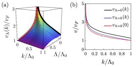
Our numerical result for in
Fig. 2 (a) clearly shows that the external momentum
replaces as effective infrared cutoff as soon as .
Figure 2: (Color online)
(a) Velocity
as a function of infrared cutoff and external momentum
obtained from the numerical solution of Eqs. (11a) and (11b).
In (b) the solid line represents our FRG result for the physical momentum-dependent velocity
as a function of .
For comparision, we also show
and .
The physical momentum-dependent velocity
is shown in Fig. 2 (b).
For comparison, we also show the
velocities
and ; the latter can also be obtained using the field-theoretical RG
if one stops the RG flow at finite and then substitutes .
While
this recipe works perfectly to leading
order in where the perturbative result for
can be obtained by replacing in Eq. (1),
we see
from Fig. 2 (b) that
this procedure remains approximately valid also
for the physically relevant .
Our FRG result for can be fitted by
,
where
and for .
Note that our result for is very close to the
first order expression .
This is surprising, because in a perturbative expansion
the second order correction
leads to an additional contribution
to the prefactor of , where
according to Mishchenko Mishchenko07 , Vafek et al.Vafek08 obtained , and Barnes et al.Barnes14 found . In any case, for
the second order correction
is substantial; our
FRG calculation suggests that in this case
the terms of order are to a large extent
cancelled by higher order corrections.
To compare our results with the experimental data for the renormalized velocity
in suspended graphene Elias11 , we need to fix the value
of the ultraviolet cutoff which appears as a free parameter
in our low-energy action (3).
Following the usual field-theoretical
procedure deJuan10 , we eliminate in favour of some measurable observable.
Note that the authors of Ref. [Elias11, ] use cyclotron resonance to measure
the quasi-particle velocity at the Fermi momentum
for different densities in slightly doped graphene.
Assuming that the function is approximately independent of
(which seems to be reasonable at low densities),
we may fix by demanding that our result for
agrees with the measured quasi-particle velocity at
one particular value of .
Here we choose the data point at
to fix ; other choices lead to fits of similar quality.
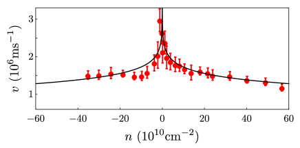
In Fig. 3 we compare the renormalized velocity obtained with
this prescription with the experimental data Elias11 .
Figure 3: (Color online)
Comparison of our FRG result
for the renormalized velocity as a function of the density
with the data from Ref. [Elias11, ] (dots with error-bars).
The ultraviolet cutoff is fixed as described in the text.
Obviously, in the entire range of available densities
our FRG result agrees quite well with the data.
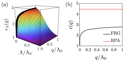
Finally, in Fig. 4 (a) we show our numerical results for the
momentum- and cutoff-dependent dielectric function
. Here the external momentum and the cutoff
do not play the same role, because the dielectric function
is defined in terms of the bosonic self-energy while the infrared cutoff
has been introduced in the fermionic propagator.
The physical dielectric function
is shown in Fig. 4 (b).
Figure 4: (Color online)
(a) Momentum- and cutoff-dependent
dielectric function
obtained from the
numerical solution of the FRG flow equations (11a) and (11b).
(b) Physical dielectric function
.
The dashed line represents the RPA result for .
Note that the logarithmic divergence of the velocity for small
leads to the logarithmic vanishing of the static bosonic self-energy , so that
the corresponding dielectric function
logarithmically approaches unity
for . Hence, in the static long-wavelength limit
the Coulomb interaction in suspended graphene is not screened at all.
On the other hand, if we replace
the flowing velocity by the bare velocity
on the right-hand side of
our flow equation (11b) and take the limit
we recover the RPA result
.
In summary, we have derived and solved non-perturbative FRG flow equations
for the momentum- and cutoff-dependent quasi-particle velocity
and the static dielectric function
of suspended graphene.
In the physical limit our result
for diverges as for and
agrees very well
with a recent experiment Elias11 .
The dielectric function is shown to approach unity for ,
in contrast to the prediction of the RPA.
Our approach can be extended in several directions:
with some extra numerical effort, the frequency-dependence of the dielectric function
can be taken into account. Moreover, we can generalize our approach to allow for
the spontaneous formation of a charge-density wave
which transforms the system into
an excitonic insulator Kotov12 ; Khveshchenko01 .
We thank A. Geim for making the data for the renormalized velocity
from Ref. [Elias11, ] available to us.
Two of us (C. B. and P. K.) acknowledge the hospitality of the
physics department of the University of Florida, Gainesville, where part of this work
has been carried out.
References
(1)
V. N. Kotov, B. Uchoa, V. M. Pereira, F. Guinea, and A. H. Castro Neto,
Rev. Mod. Phys. 84, 1067 (2012).
(2)
D. C. Elias, R. V. Gorbachev, A. S. Mayorov, S. V. Morozov,
A. A. Zhukov, P. Blake, L. A. Ponomarenko,
I. V. Grigorieva, K. S. Novoselov, F. Guinea, and A. K. Geim,
Nat. Phys. 7, 701 (2011).
(3)
D. A. Siegel, C. H. Park, C. Hwang, J. Deslippe, A. V. Fedorov, S. G. Louie, and A. Lanzara, Proc. Natl. Acad. Sci. U.S.A. 108, 11365
(2011).
(4)
G. L. Yu, R. Jalil, B. Belle, A. S. Mayorov, P. Blake, F. Schedin, S. V. Morozov, L. A. Ponomarenko, F. Chiappini, S. Wiedmann, U. Zeitler, M. I. Katsnelson, A. K. Geim, K. S. Novoselov, and D. C. Elias, Proc. Natl. Acad. Sci. U.S.A. 110, 3282 (2013).
(5)
J. Gonzalez, F. Guinea, and M. A. H. Vozmediano,
Nucl. Phys. B 424, 595 (1994).
(6)
P. Kopietz, L. Bartosch, and F. Schütz, Introduction to the
Functional Renormalization Group (Springer, Berlin, 2010).
(7)
W. Metzner, M. Salmhofer, C. Honerkamp, V. Meden, and K. Schönhammer,
Rev. Mod. Phys. 84, 299 (2012).
(8)
C. Wetterich, Phys. Lett. B 301, 90 (1993).
(9)
F. Schütz, L. Bartosch, and P. Kopietz,
Phys. Rev. B 72, 035107 (2005).
(10)
D. Sheehy and J. Schmalian, Phys. Rev. Lett. 99, 226803 (2007).
(11)
J. Gonzalez, Phys. Rev. B 82, 155404 (2010).
(12)
V. N. Kotov, B. Uchoa, and A. H. Castro Neto, Phys. Rev. B 78, 035119 (2008).
(13)
J. Hofmann, E. Barnes, and S. Das Sarma,
Phys. Rev. Lett. 113, 105502 (2014).
(14)
E. Barnes, E. H. Hwang, R. E. Thockmorton, and S. Das Sarma,
Phys. Rev. B 89, 235431 (2014).
(15)
O. Vafek and M. J. Case, Phys. Rev. B 77, 033410 (2008).
(16)
E. G. Mishchenko, Phys. Rev. Lett. 98, 216801 (2007).
(17)
F. de Juan, A. G. Grushin, and M. A. H. Vozmediano, Phys. Rev. B 82, 125409 (2010).
(18)
D. V. Khveshchenko, Phys. Rev. Lett. 87, 246802 (2001).