Generation of a Novel Exactly Solvable Potential

Abstract

We report a new shape invariant (SI) isospectral extension of the Morse potential. Previous investigations have shown that the list of “conventional” SI superpotentials that do not depend explicitly on Planck’s constant $\hbar$ is complete. Additionally, a set of “extended” superpotentials has been identified, each containing a conventional superpotential as a kernel and additional $\hbar$-dependent terms. We use the partial differential equations satisfied by all SI superpotentials to find a SI extension of Morse with novel properties. It has the same eigenenergies as Morse but different asymptotic limits, and does not conform to the standard generating structure for isospectral deformations.

1 Introduction

Supersymmetric quantum mechanics [1, 2, 3] generalizes the familiar factorization method for the harmonic oscillator. A general hamiltonian $H_{-}$ is factorized in terms of two operators ${\cal A}^{+}\equiv-\hbar\frac{d}{dx}+W(x,a)$ and ${\cal A}^{-}\equiv\hbar\frac{d}{dx}+W(x,a)$, where the function $W(x,a)$ is known as the superpotential. We have set the mass $m=1/2$. The product ${\cal A}^{+}\,{\cal A}^{-}$ is then given by

$${\cal A}^{+}\,{\cal A}^{-} = \left(-\hbar\frac{d}{dx}+W(x,a)\right)~{}\left(\hbar\frac{d}{dx}+W(x,a)\right)$$ (1)

$$= -\hbar^{2}\frac{d^{2}}{dx^{2}}+W^{2}(x,a)-\hbar\frac{d\,W(x,a)}{dx}~{},$$

This product ${\cal A}^{+}\,{\cal A}^{-}$ produces a hamiltonian $H_{-}=-\hbar^{2}\frac{d^{2}}{dx^{2}}+V_{-}(x,a)$, where $V_{-}(x,a)=W^{2}(x,a)-\hbar\frac{d\,W(x,a)}{dx}$. A product of operators ${\cal A}^{-}$ and ${\cal A}^{+}$ carried out in the reverse order produces another hamiltonian $H_{+}=-\hbar^{2}\frac{d^{2}}{dx^{2}}+V_{+}(x,a)$ with $V_{+}(x,a)=W^{2}(x,a)+\hbar\frac{d\,W(x,a)}{dx}$. The two hamiltonians are intertwined; i.e., ${\cal A}^{+}H_{+}=H_{-}{\cal A}^{+}$ and ${\cal A}^{-}H_{-}=H_{+}{\cal A}^{-}$. This leads to the following isospectrality relationships among their eigenvalues and eigenfunctions for all integer $n\geq 0$:

$$E^{-}_{n+1}=E^{+}_{n},$$ (2)

$$\frac{~{}~{}~{}{\cal A}^{-}}{\sqrt{E^{+}_{n}}}~{}\psi^{(-)}_{n+1}=~{}\psi^{(+)}_{n}~{}{\rm,and}~{}\frac{~{}~{}~{}{\cal A}^{+}}{\sqrt{E^{+}_{n}}}~{}\psi^{(+)}_{n}=~{}\psi^{(-)}_{n+1}.$$ (3)

Eq. (3) implies that if somehow we knew the eigenvalues and eigenstates of the hamiltonian $H_{-}$, we would automatically know the same for the hamiltonian $H_{+}$, and vice-versa.

We can go no further unless we know the spectrum for one of the potentials a priori. However, if the superpotential $W(x,a_{i})$ obeys the following “shape invariance condition” [4, 5, 6, 7],

$$W^{2}(x,a_{i})+\hbar\frac{d\,W(x,a_{i})}{dx}+g(a_{i})=W^{2}(x,a_{i+1})-\hbar\frac{d\,W(x,a_{i+1})}{dx}+g(a_{i+1}),~{}$$ (4)

the eigenvalues and eigenfunctions for both hamiltonians can be determined separately. In this letter we consider the case of translational or additive shape invariance: $a_{i+1}=a_{i}+\hbar$. From Eq. (4) it follows that for a shape invariant system the partner hamiltonians $H_{+}(x,a_{i})$ and $H_{-}(x,a_{i+1})$ differ only by values of parameter $a_{i}$ and additive constants $g(a_{i})$. The eigenvalues and eigenfunctions of a shape invariant system are then given by [8, 9]

$$E_{n}^{(-)}(a_{0})=g(a_{n})-g(a_{0})~{}~{}{\rm for}~{}n\geq 0~{},$$

and

$$\psi^{(-)}_{n}(x,a_{0})=\frac{{\cal A}^{+}{(a_{0})}~{}{\cal A}^{+}{(a_{1})}\cdots{\cal A}^{+}{(a_{n-1})}~{}\psi^{(-)}_{0}(x,a_{n})}{\sqrt{E_{n}^{(-)}(a_{0})\,E_{n-1}^{(-)}(a_{1})\cdots E_{1}^{(-)}(a_{n-1})}}~{},$$

where $\psi^{(-)}_{0}(x,a_{n})=Ne^{-\frac{1}{\hbar}\,\int^{x}W(y,a_{n})\,dy}$ is the solution of ${\cal A}^{-}\psi^{(-)}_{0}=0$ and $N$ is the normalization constant. Thus, all additive shape invariant systems are exactly solvable. Therefore, finding all such potentials gives important insight into the nature of quantum mechanical systems. Previously, researchers found a list of additive shape invariant potentials, generally by trial and error [4, 10, 11]. In Ref. [12, 13] the authors showed that all “conventional” ($\hbar$-independent) shape invariant superpotentials could be determined as solutions to a set of two partial differential equations. Additionally, they showed that the list of conventional shape invariant superpotentials given in Ref.[10] was indeed complete.

A new class of “extended” superpotentials was discovered [14, 15] and expanded upon [16, 17, 18, 19, 20, 21, 22, 23, 24]. These superpotentials contain explicit $\hbar$-dependence in $W$. When expanded in powers of $\hbar$, each power of $\hbar$ yields a new partial differential equation that must be satisfied by these superpotentials [12, 13].

Although this formalism has been checked for consistency with already known superpotentials [12, 13], it has not been used to generate a new superpotential. In this letter we employ it to generate an extension of the Morse superpotential. This extended superpotential exhibits properties that are qualitatively different from those previously discovered. It has different asymptotic values than Morse and it contains free parameters.

2 A Novel Potential

We first consider conventional superpotentials that do not have an intrinsic dependence on $\hbar$. Note that in Eq. (4), for additive shape invariance the constant $\hbar$ enters $W$ through the linear combination $a+\hbar$; therefore, $\frac{\partial}{\partial\hbar}W(x,a+\hbar)=\frac{\partial}{\partial a}W(x,a+\hbar)$. Since Eq. (4) must hold for an arbitrary value of $\hbar$, we can expand it in powers of $\hbar$, and stipulate that the coefficient of each power vanishes. This leads to two independent equations [12, 13]:

$$\vspace{6pt}W\,\frac{\partial W}{\partial a}-\frac{\partial W}{\partial x}+\frac{1}{2}\,\frac{dg(a)}{da}=0~{}$$ (5)

and

$$\frac{\partial^{3}}{\partial a^{2}\partial x}~{}W(x,a)=0~{}.$$ (6)

The general solution to Eq. (6) is

$$W(x,a)=a\cdot{X}_{1}(x)+{X}_{2}(x)+u(a)~{},$$ (7)

where $X_{1},X_{2}$, and $u$ are arbitrary functions. When combined with Eq. (5), this general solution reproduces the complete family of conventional superpotentials, as shown in Table 1 [12, 13].

Name	Superpotential
Harmonic Oscillator	$\frac{1}{2}\omega x$
Coulomb	$\frac{e^{2}}{2(\ell+1)}-\frac{\ell+1}{r}$
3-D oscillator	$\frac{1}{2}\omega r-\frac{\ell+1}{r}$
Morse	$A-Be^{-x}$
Rosen-Morse I	$-A\cot x-\frac{B}{A}$
Rosen-Morse II	$A\tanh x+\frac{B}{A}$
Eckart	$-A\coth x+\frac{B}{A}$
Scarf I	$A\tan x-B{\rm sec}\,x$
Scarf II	$A\tanh x+B{\rm sech}\,x$
Gen. Pöschl-Teller	$A\coth x-B{\rm cosech}\,x$

Table 1: The complete family of $\hbar$-independent additive shape-invariant superpotentials.

The additional set of extended superpotentials reported in [14, 15] obey the shape invariance condition given in Eq. (4) only when their $W$’s depend explicitly on $\hbar$. Each of these extended superpotentials is isospectral with one of the conventional superpotentials listed in Table 1.

To determine the differential equations obeyed by extended superpotentials, we expand the superpotentials in powers of $\hbar$. I.e., we define

$$\vspace{6pt}W(x,a,\hbar)=\sum_{j=0}^{\infty}\hbar^{j}W_{j}(x,a).~{}$$ (8)

Since $a_{0}=a$ and $a_{1}=a+\hbar$, this power series yields

$$W\left(x,a_{1},\hbar\right)=\sum_{j=0}^{\infty}\sum_{k=0}^{j}\frac{\hbar^{j}}{k!}\frac{\partial^{k}W_{j-k}}{\partial a^{k}},$$

$$W^{2}\left(x,a_{1},\hbar\right)=\sum_{j=0}^{\infty}\sum_{s=0}^{j}\sum_{k=0}^{s}\frac{\hbar^{j}}{\left(j-s\right)!}\frac{\partial^{j-s}\left(W_{k}W_{s-k}\right)}{\partial a^{j-s}},$$

and

$$\left.\frac{\partial W}{\partial x}\right|_{a=a_{1}}=\sum_{j=0}^{\infty}\sum_{k=0}^{j}\frac{\hbar^{j}}{k!}\frac{\partial^{k+1}W_{j-k}}{\partial a^{k}\partial x}~{}~{}.$$

We then substitute these into Eq. (4) and demand that the equation hold for any value of $\hbar$. This is possible only if the coefficients of the series for each power of $\hbar$ are identically zero. We obtain for $j=1$

$$2\frac{\partial W_{0}}{\partial x}-\frac{\partial}{\partial a}\left(W_{0}^{2}+g\right)=0,$$ (9)

for $j=2$

$$\frac{\partial W_{1}}{\partial x}-\frac{\partial}{\partial a}\left(W_{0}\,W_{1}\right)=0,$$ (10)

and for $j\geq 3$

$$2\,\frac{\partial W_{j-1}}{\partial x}-\sum_{s=1}^{j-1}\sum_{k=0}^{s}\frac{1}{(j-s)!}\frac{\partial^{j-s}}{\partial a^{j-s}}W_{k}\,W_{s-k}+$$

$$\sum_{k=2}^{j-1}\frac{1}{(k-1)!}\frac{\partial^{k}\,W_{j-k}}{\partial a^{k-1}\,\partial x}+\left(\frac{j-2}{j!}\right)\,\frac{\partial^{j}W_{0}}{\partial a^{j-1}\partial x}=0~{}.$$ (11)

These equations appear to differ from similar equations in Ref. [12, 13], but they are in fact equivalent.

We first observe that Eq. (9) is identical to Eq. (5), i.e., all conventional shape invariant potentials automatically satisfy Eq. (9). Hence, conventional superpotentials can be used as kernels to build extended superpotentials. If $W_{0}$ is a conventional superpotential, then Eq. (6) is automatically satisfied for $W_{0}$, meaning that the last term of Eq. (11) disappears.

In the remainder of this paper, we use the Morse superpotential as a kernel to construct an extended superpotential. In Ref. [22], the author generated a quasi-exactly solvable extension of Morse and showed that it was not shape invariant.

The strength of the method used in this letter is that we can employ Eq. (11) term-by-term in order to generate a manifestly shape-invariant solution. Hence, we begin with $W_{0}=(\alpha-a)-e^{-x}$ and choosing $W_{1}=0$, the equation for $W_{2}$ reads

$$\frac{\partial W_{2}}{\partial x}-\frac{\partial W_{0}W_{2}}{\partial a}=0.$$

This equation is solved by

$$W_{2}(x,a)=e^{-x}\left(2P+Qe^{-2x}-2\left(\alpha-a\right)Qe^{-x}\right)~{},$$

where $P$ and $Q$ are constant parameters. Assuming $W_{3}$ to be zero, the equation for $W_{4}$ is

$$2\frac{\partial W_{4}}{\partial x}-2\frac{\partial\left(W_{0}W_{4}+\frac{1}{2}W_{2}^{2}\right)}{\partial a}-\frac{\partial}{\partial a}\left(\frac{\partial W_{2}}{\partial a}\frac{\partial W_{0}}{\partial a}\right)-$$

$$\frac{1}{3}\left(W_{2}\frac{\partial^{3}W_{0}}{\partial a^{3}}+W_{0}\frac{\partial^{3}W_{2}}{\partial a^{3}}\right)+\frac{1}{2}\frac{\partial^{3}W_{2}}{\partial x\partial a^{2}}=0~{}.$$

The above equation is solved by

$$W_{4}(x,a)=-Qe^{-3x}\left(2P+Qe^{-2x}-2\left(\alpha-a\right)Qe^{-x}\right)~{}.$$

Generalizing this process yields $W_{2k-1}=0$ and

$$W_{2k}=\left(-Q\right)^{k-1}e^{-(2k-1)x}\left(2P+Qe^{-2x}-2\left(\alpha-a\right)Qe^{-x}\right)$$

for all positive integers $k.$ Computing the infinite sum $\sum_{j=0}^{\infty}\hbar^{j}W_{j}(x,a)$, we obtain

$$W(x,a,\hbar)=(\alpha-a)-e^{-x}+\frac{\hbar^{2}\left(2Pe^{x}-2\left(\alpha-a\right)Q+Qe^{-x}\right)}{e^{2x}+Q\,\hbar^{2}}~{}.$$ (12)

The shape invariance of a superpotential of this form can be directly checked. Substituting the above expression into Eq. (4) yields

$$W^{2}(x,a)-W^{2}(x,a+\hbar)+\hbar\frac{d\,}{dx}\left(W(x,a)+W(x,a+\hbar)\right)=\hbar(2(\alpha-a)-\hbar),$$ (13)

which can be brought into the form of Eq. (4) by choosing $g(a)=-(\alpha-a)^{2}$. This leads to the energy eigenvalues $E^{(-)}_{n}=g(a+n\hbar)-g(a)=(\alpha-a)^{2}-(\alpha-a-n\hbar)^{2}$. These values are exactly the same as those of the Morse potential. Figs. (1) and (2) show $W$ and the partner potentials $V_{-}$ and $V_{+}$, where we have chosen the specific values $A=3,B=5,\alpha=5,a=2$, and $\hbar=1$, as an example. Asymptotic limits for this extended superpotential are finite and their absolute values are equal. Consequently, the resulting potential has identical limits at $\pm\infty$.

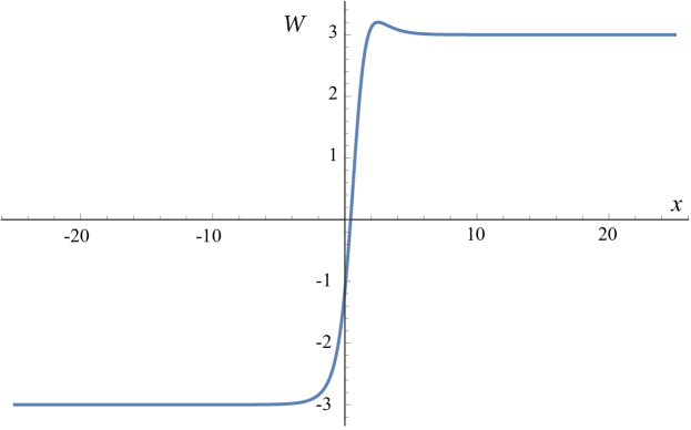
Figure 1: Superpotential $W$ for $P=3,Q=5,\alpha=5,a=2$, and $\hbar=1.$ Its asymptotic values imply an unbroken supersymmetry.

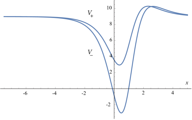
Figure 2: Potentials $V_{-}$ and $V_{+}$ for the same values of the parameters as Fig. 1. The deeper potential is $V_{-}$, and it holds the zero-energy groundstate.

The ground state eigenfunction can be obtained from the first order differential equation $\mathcal{A}^{-}(x,a)\,\psi_{0}(x,a)=0$, yielding

$$\psi_{0}(x,a)=N\left(\hbar^{2}Q+e^{2x}\right)^{a-\alpha}\exp\left[x(\alpha-a)+\frac{\left(1-2\hbar^{2}P\right)\tan^{-1}\left(\frac{e^{x}}{\hbar\sqrt{Q}}\right)}{\hbar\sqrt{Q}}\right],$$

where $N$ is the normalization constant. The excited states can be obtained recursively by applying the $\mathcal{A}^{+}$ operator to $\psi_{0}$. The first excited state is $\psi_{1}(x,a)=\mathcal{A}^{+}(x,a)\psi_{0}(x,a+\hbar)/\sqrt{E_{1}}$, and so on. For example, with our particular choice of parameters, the potential $V_{-}(x)$ holds three bound states, corresponding to the eigenenergies $0,5$ and $8$. The fourth energy level is at $9$, which does not hold a bound state. We obtain for the ground state eigenfunction

$$\psi_{0}(x)=\frac{40}{\left(e^{2x}+5\right)^{3}}\sqrt{\frac{105}{1+e^{-\sqrt{5}\pi}}}\exp\left[3x-\sqrt{5}\tan^{-1}\left(\frac{e^{x}}{\sqrt{5}}\right)\right],$$

and for the first two excited states

$$\psi_{1}(x)=\frac{20\left(\,e^{2x}+2e^{x}-5\right)\sqrt{\frac{70}{1+e^{\sqrt{5}\pi}}}\,}{\left(e^{2x}+5\right)^{3}}\exp\left[{2x-\sqrt{5}\tan^{-1}\left(\frac{e^{x}}{\sqrt{5}}\right)+\frac{\sqrt{5}\pi}{2}}\right],$$

$$\psi_{2}(x)= \frac{4\left(3e^{4x}+20e^{3x}-20e^{2x}-100e^{x}+75\right)\sqrt{\frac{5}{1+e^{\sqrt{5}\pi}}}}{\left(e^{2x}+5\right)^{3}}$$

$$\times\exp\left[x-\sqrt{5}\tan^{-1}\left(\frac{e^{x}}{\sqrt{5}}\right)+\frac{\sqrt{5}\pi}{2}\right].$$

As expected, the fourth energy level does not hold a bound state, as its corresponding eigenfunction is not square integrable. Fig. (3) superimposes over the potential $V_{-}(x)$ the three bound-state eigenfunctions together with their corresponding eigenenergies.

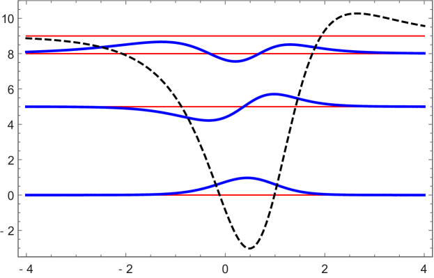
Figure 3: The three bound-state eigenfunctions (shown in blue) for $V_{-}$ (dashed line) with $P=3,Q=5,\alpha=5,a=2$, and $\hbar=1.$ Each eigenfunction is shown superposed on its corresponding eigenenergy (shown as a horizontal red line).

As $\hbar\rightarrow 0$, this transforms into the Morse potential, as expected. In addition, parameters $P$ and $Q$ also allow us to deform the potential away from the Morse potential without affecting its eigenvalues. In this sense, we can consider it to be a shape-invariant isospectral deformation of Morse.

3 Conclusions

In this letter, we have shown that the partial differential equations (11) can be used to generate a shape invariant extension of the Morse superpotential, whose asymptotic limits differ from those of Morse. In addition, the free parameters available in this model allow for its isospectral deformation away from Morse.

References

References

- [1] E. Witten, Dynamical breaking of supersymmetry, Nucl. Phys. B185 (1981) 513–554.
- [2] P. Solomonson, J. W. Van Holten, Fermionic coordinates and supersymmetry in quantum mechanics, Nucl. Phys. B196 (1982) 509–531.
- [3] F. Cooper, B. Freedman, Aspects of supersymmetric quantum mechanics, Ann. Phys. 146 (1983) 262–288.
- [4] L. Infeld, T. E. Hull, The factorization method, Rev. Mod. Phys. 23 (1951) 21–68.
- [5] W. Miller Jr, Lie Theory and Special Functions (Mathematics in Science and Engineering), Accademic Press, New York, NY, USA, 1968.
- [6] L. E. Gendenshtein, Derivation of exact spectra of the schrodinger equation by means of supersymmetry, JETP Lett. 38 (1983) 356–359.
- [7] L. E. Gendenshtein, I. V. Krive, Supersymmetry in quantum mechanics, Sov. Phys. Usp. 28 (1985) 645–666.
- [8] F. Cooper, A. Khare, U. Sukhatme, Supersymmetry in Quantum Mechanics, World Scientific, Singapore, 2001.
- [9] A. Gangopadhyaya, J. Mallow, C. Rasinariu, Supersymmetric Quantum Mechanics: An Introduction, World Scientific, Singapore, 2010.
- [10] R. Dutt, A. Khare, U. Sukhatme, Supersymmetry, shape invariance and exactly solvable potentials, Am. J. Phys. 56 (1988) 163–168.
- [11] F. Cooper, J. Ginocchio, A. Khare, Relationship between supersymmetry and solvable potentials, Phys. Rev. D 36 (1987) 2458–2473.
- [12] J. Bougie, A. Gangopadhyaya, J. V. Mallow, Generation of a complete set of additive shape-invariant potentials from an euler equation, Phys. Rev. Lett. (2010) 210402:1–210402:4.
- [13] J. Bougie, A. Gangopadhyaya, J. V. Mallow, C. Rasinariu, Supersymmetric quantum mechanics and solvable models, Symmetry 4 (3) (2012) 452–473.
- [14] C. Quesne, Exceptional orthogonal polynomials, exactly solvable potentials and supersymmetry, J. Phys. A 41 (2008) 392001:1–392001:6.
- [15] C. Quesne, Solvable rational potentials and exceptional orthogonal polynomials in supersymmetric quantum mechanics, Sigma 5 (2009) 084:1–084:24.
- [16] S. Odake, R. Sasaki, Infinitely many shape invariant discrete quantum mechanical systems and new exceptional orthogonal polynomials related to the wilson and askey-wilson polynomials, Phys. Lett. B 682 (2009) 130–136.
- [17] S. Odake, R. Sasaki, Another set of infinitely many exceptional laguerre polynomials, Phys. Lett. B 684 (2010) 173–176.
- [18] T. Tanaka, N-fold supersymmetry and quasi-solvability associated with x-2-laguerre polynomials, J. Math. Phys. 51 (2010) 032101:1–032101:20.
- [19] S. Odake, R. Sasaki, Exactly solvable quantum mechanics and infinite families of multi-indexed orthogonal polynomials, Phys. Lett. B 702 (2011) 164–170.
- [20] R. Odake, S.and Sasaki, Extensions of solvable potentials with finitely many discrete eigenstates, J. Phys. A 46 (2013) 235205.
- [21] C. Quesne, Novel enlarged shape invariance property and exactly solvable rational extensions of the rosen-morse ii and eckart potentials, Sigma 8 (2012) 080.
- [22] C. Quesne, Revisiting (quasi-)exactly solvable rational extensions of the morse potential, Int. J. Mod. Phys. A 27 (2012) 1250073.
- [23] S. Sree Ranjani, P. K. Panigrahi, A. K. Kapoor, A. Khare, A. Gangopadhyaya, Exceptional orthogonal polynomials, qhj formalism and swkb quantization condition, Jour. of Phys. A 45 (2012) 055210.
- [24] S. Sree Ranjani, R. Sandhya, A. K. Kapoor, Shape invariant rational extensions and potentials related to exceptional polynomials, arXiv:1503.01394.