Full counting statistics of Majorana interferometers

Abstract

We study the full counting statistics of interferometers for chiral Majorana fermions with two incoming and two outgoing Dirac fermion channels. In the absence of interactions, the FCS can be obtained from the $4\times 4$ scattering matrix $S$ that relates the outgoing Dirac fermions to the incoming Dirac fermions. After presenting explicit expressions for the higher-order current correlations for a modified Hanbury Brown-Twiss interferometer, we note that the cumulant-generating function can be interpreted such that unit-charge transfer processes correspond to two independent half-charge transfer processes, or alternatively, to two independent electron-hole conversion processes. By a combination of analytical and numerical approaches, we verify that this factorization property holds for a general $SO(4)$ scattering matrix, i.e. for a general interferometer geometry.

1 Introduction

In a seminal work Büttiker pointed out the power of investigating non-local current correlations in mesoscopic conductors to detect particle exchange effects [1]. This work extended the scope of previous studies of shot noise in two-terminal conductors [2, 3, 4, 5] by showing that fundamental quantum mechanical effects can play a decisive role in electronic transport properties.

Later on, Büttiker demonstrated on completely general grounds that cross-correlations of bosonic and fermionic free particles are fundamentally different [6]. Whereas for bosons the sign is determined by the competition between positively contributing bunching effects and negatively contributing partitioning effects, free fermions always exhibit overall negative cross-correlations due to their antibunching property. Thus, the observation of positive cross-correlations for fermions requires some nontrivial interaction between them. A first example was provided by a superconducting source injecting currents into two normal leads [7, 8]. Surprisingly, the effect persists even for many-channel conductors [9, 10]. Furthermore, strong Coulomb interactions can also impose positive cross-correlations in multi-terminal quantum dot systems [11, 12]. An analysis of the full counting statistics reveals a dynamical bunching effect as the origin of the positive cross-correlations [9, 13].

Because of their fascinating properties and potential applications in topological quantum information [14, 15, 16, 17, 18], Majorana fermions in condensed-matter systems have attracted a great deal of interest. However, their unambiguous detection in experiments has remained a difficult task: they are chargeless and – like the Laughlin quasiparticles in the fractional quantum Hall effect – cannot be extracted from their many-body environment. Elaborate schemes leading to indirect but conclusive signatures of their presence have been proposed and partially realized.

Recently, several groups [19, 20] have reported the identification of Majorana bound states in nanowires by observing a zero-bias peak in tunneling spectroscopy experiments. There is, however, no consensus regarding the attribution of this result to the presence of Majorana fermions. The situation is similar with the experimental report [21] of a 4$\pi$-periodic Josephson effect, which cannot yet be unambiguously attributed to the presence of Majorana bound states in the Josephson junction.

There are also many proposals to detect Majorana fermions based on interferometric structures. They can be divided into two classes. The first class intends to probe the non-Abelian statistics of Majorana bound states trapped in vortices of topological superconductors. In Ref. [22, 23] the authors study conductance signatures of vortex tunneling in a Fabry-Pérot interferometer. Another proposal [24] is based on a Mach-Zehnder interferometer constructed from a topological Josephson junction. In that case, Josephson vortices trapping a Majorana bound state propagate along the two arms of the interferometer and give rise to a Josephson-vortex current $I_{v}$. The presence of absence of another MBS at the center of the interferometer, which can be tuned by a magnetic flux, leads to a striking switching between a vanishing $I_{v}$ and a nonzero $I_{v}$. The roots of this effect are traced back to the non-Abelian exchange statistics of Majorana bound states.

The goal of the second class of interferometer-based proposals is to find a signature of Majorana edge states [22, 25, 26, 27, 28, 29]. They propose to use 3D topological insulator heterostructures to build a Mach-Zehnder interferometer for Majorana edge states contacted by electronic leads and find conductance signatures. Reference [26] finds a signature of chiral Majorana modes in the conductance of a Mach-Zehnder interferometer built in a superconductor–quantum spin Hall–superconductor sandwich.

Büttiker et al. [29] introduced a powerful scattering matrix approach in terms of Majorana modes that highlights their special properties and is readily applied to these interferometric structures.

Motivated by these works, in Ref. [27] this setup was extended to interferometers with two incoming and two outgoing Dirac fermion channels. Furthermore it was proposed to study noise correlations in a Hanbury Brown-Twiss (HBT) type interferometer, and three signatures of the Majorana nature of the channels were predicted. First, the average charge current in the outgoing leads vanishes. Furthermore, an anomalously large shot noise in the output ports for a vanishing average current signal is expected. Adding a quantum point contact (QPC) to the setup, a surprising absence of partition noise was found which can be traced back to the Majorana nature of the carriers.

In view of previous successes of studies of higher-order correlators [30, 31, 32, 9] it is natural to ask [33, 34] if other Majorana signatures could be hidden in higher-order correlations. Therefore we will investigate the full counting statistics in multi-terminal structures containing Majorana modes to access correlations beyond noise.

In Ref. [35], the full counting statistics was calculated for a network of localized Majorana bound states coupled by tunneling. In this work, in contrast, we will use full counting statistics to focus on the transport in systems containing one-dimensional, propagating Majorana modes.

2 Scattering matrix and full counting statistics (FCS)

A very general description of quantum transport in a multi-terminal device is to calculate the full counting statistics (FCS) of the transfered charges, which contains the full information about the current and higher-order current-current correlation functions at zero frequency. Let us denote the probability that $N_{1},N_{2},\ldots$ charges are transported into terminal $1,2,\ldots$ during a fixed measurement time by $P(N_{1},N_{2},\ldots)$. A quantity which is equivalent but easier to calculate is the cumulant generating function (CGF), defined by $\ln\chi(\lambda_{1},\lambda_{2},\ldots)=\ln\langle\exp(i\lambda_{1}N_{1}+i\lambda_{2}N_{2}+\cdots)\rangle$, where the average denotes the statistical average with the probability $P$.

FCS helps to understand transport because it allows an identification of elementary transport events by decomposing the CGF into a sum of multinomial distributions, where the sum indicates the independence of the various transport processes in the long-time limit.

Our goal is to study Majorana interferometers like, e.g., the Hanbury Brown-Twiss interferometer with the additional QPC, see Fig. 1 and [27].

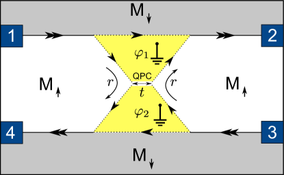
Figure 1: Modified Hanbury Brown-Twiss interferometer, see [27]. Majorana excitations will propagate along the boundaries of the two triangular superconducting structures with phases $\varphi_{1}$, $\varphi_{2}$. An additional short gapped channel appears at the domain wall between the two superconducting regions, forming a quantum point contact characterized by reflection and transmission amplitudes $r$, $t$. The setup is similar to the one proposed in [25].

In the absence of interactions, the FCS can be obtained from the $4\times 4$ scattering matrix $S$ that relates the outgoing Dirac fermions to the incoming Dirac fermions in the following way

$$\left(\begin{array}[]{c}\psi_{2,e}\\ \psi_{2,h}\\ \psi_{4,e}\\ \psi_{4,h}\end{array}\right)=S\left(\begin{array}[]{c}\psi_{1,e}\\ \psi_{1,h}\\ \psi_{3,e}\\ \psi_{3,h}\end{array}\right)\>,$$ (9)

where $1,3$ label the incoming channels, $2,4$ the outgoing channels, $e$ denotes an electronic mode, and $h$ denotes a hole mode.

The matrix elements of the scattering matrix represent the probability amplitude of different “processes”. For instance, the matrix element $s_{11}$ is the probability amplitude that an incoming electron in lead 1 goes out as an electron in lead $2$; and $s_{34}$ is the probability amplitude that an incoming hole in lead 3 goes out as an electron in lead 4. The matrix elements already contain all the interference effects of single-particle states.

Two-particle processes: To obtain the probability amplitudes for two-particle states, we must take anti-symmetric combinations of products of matrix elements. For instance, the probability amplitude that two incoming electrons in leads $1$ and $3$ go out as electrons in leads $2$ and $4$ is given by $s_{11}s_{33}-s_{13}s_{31}$, i.e., the probability amplitude that the incoming electron in lead 1 goes out as an electron in lead 2 AND the incoming electron in lead 3 goes out as an electron in lead 4, MINUS the probability amplitude that the incoming electron in lead 3 goes out as an electron in lead 2 AND the incoming electron in lead 1 goes out as an electron in lead 4. These two processes interfere and lead to effects such as the two-particle Aharonov-Bohm effect [36].

Three-particle processes: It is also possible to have three-particle processes: an incoming lead populated by both an electron and a hole, the other incoming lead populated by either an electron or a hole.

Four-particle process: There is only one such process: all the incoming states and all the outgoing states are totally filled. This (trivial) process occurs with probability amplitude $\det S=1$ (or probability $|\det S|^{2}=1$).

To obtain the full counting statistics we sum up the contributions of all these coherent processes weighted by the probability of the input states (occupation of the incoming leads). For instance, the probability $P_{ij}$ of obtaining two particles in the outgoing modes $i,j\in\{1,\ldots 4\}$ is

$$P_{ij}=\frac{1}{2}\sum_{k,l=1}^{4}\left|s_{ik}s_{jl}-s_{il}s_{jk}\right|^{2}n_{k}n_{l}(1-n_{a})(1-n_{b})\>,$$ (10)

where $k,l$ run over the incoming modes, and $n_{k}$ is the occupation of the incoming mode $k$. The indices $a$ and $b$ are the two remaining incoming modes (such that the set $\{a,b,k,l\}=\{1,2,3,4\}$). The factor $1/2$ is inserted to avoid double counting.

A measurement of the current and its correlation function will not make is possible to determine all entries of the matrix $P_{ij}$ because, e.g., processes with no charge going out at all are not distinguishable from processes where both an electron and a hole go out into the same lead. Therefore, the FCS is characterized by only nine independent probabilities:

• $P_{00}$, no net charge in the outgoing leads,

• $P_{\pm 0}$, an electron (hole) in the outgoing lead 2,

• $P_{0\pm}$, an electron (hole) in the outgoing lead 4,

• $P_{\pm\pm}$, an electron (hole) in both outgoing leads,

• $P_{\pm\mp}$, an electron (hole) in outgoing lead 2 and a hole (electron) in outgoing lead 4.

All of these probabilities can be conveniently retrieved from the scattering matrix and the occupation of the leads. The cumulant generating function is $\ln\chi(\lambda_{2},\lambda_{4})$, where $\lambda_{i}$ is the counting field of outgoing charge in lead $i$, and

$$\chi(\lambda_{2},\lambda_{4})=\sum_{s_{2},s_{4}=-,0,+}P_{s_{2}s_{4}}e^{ie(s_{2}\lambda_{2}+s_{4}\lambda_{4})}\>.$$ (11)

Since we treat the leads as free fermion reservoirs the knowledge of the probabilities allows to directly access the FCS. The cumulant generating function can be alternatively obtained from the Levitov-Lesovik determinant formula [30, 37], which can easily be shown to lead to the same result.

3 FCS of the Hanbury Brown-Twiss interferometer

To analyze the full counting statistics of the Hanbury Brown-Twiss interferometer of Majorana fermions shown in Fig. 1, we insert the appropriate expression for the scattering matrix [27]

$$\left(\begin{array}[]{c}\psi_{2,e}\\ \psi_{2,h}\\ \psi_{4,e}\\ \psi_{4,h}\end{array}\right)=\frac{1}{2}\left(\begin{array}[]{cccc}\eta_{1}-t&\eta_{1}+t&r&r\\ \eta_{1}+t&\eta_{1}-t&-r&-r\\ r&-r&-\eta_{2}+t&\eta_{2}+t\\ r&-r&\eta_{2}+t&-\eta_{2}+t\end{array}\right)\left(\begin{array}[]{c}\psi_{1,e}\\ \psi_{1,h}\\ \psi_{3,e}\\ \psi_{3,h}\end{array}\right).$$ (12)

into Eqs. (10) and (11). The probabilities are related to charge transfer processes of the structure. The probability $P_{0,0}$ does not contribute to the sum in Eq. (11) because it corresponds to processes where no net charge is transmitted to either lead 2 or 4. The remaining probabilities are given by

$$P_{\pm,0}= \frac{1}{8}-2\alpha\beta\gamma\delta\pm\frac{1}{4}t\ \mathrm{Re}(\eta_{1})(\alpha-\beta)(4\gamma\delta+1)+\frac{1}{2}t^{2}\ (\gamma\delta-\alpha\beta)\>,$$

$$P_{0,\pm}= \frac{1}{8}-2\alpha\beta\gamma\delta\pm\frac{1}{4}t\ \mathrm{Re}(\eta_{2})(\gamma-\delta)(4\alpha\beta+1)+\frac{1}{2}t^{2}\ (\alpha\beta-\gamma\delta)\>,$$

$$P_{\pm,\pm}= \frac{1}{16}+\alpha\beta\gamma\delta-\frac{1}{8}(\alpha+\beta)(\gamma+\delta)+\frac{1}{8}\mathrm{Re}(\eta_{1}\eta_{2})(\alpha-\beta)(\gamma-\delta)$$

$$\pm\frac{1}{8}t\left(\mathrm{Re}(\eta_{1})(\alpha-\beta)(1-4\gamma\delta)+\mathrm{Re}(\eta_{2})(\gamma-\delta)(1-4\alpha\beta)\right)$$

$$+\frac{1}{8}t^{2}\left(\mathrm{Re}(\eta_{1}\eta_{2}^{*})(\alpha-\beta)(\gamma-\delta)-(\alpha-\gamma)(\beta-\delta)-(\alpha-\delta)(\beta-\gamma)\right)\>,$$

$$P_{\pm,\mp}= \frac{1}{16}+\alpha\beta\gamma\delta-\frac{1}{8}(\alpha+\beta)(\gamma+\delta)-\frac{1}{8}\mathrm{Re}(\eta_{1}\eta_{2})(\alpha-\beta)(\gamma-\delta)$$

$$\pm\frac{1}{8}t\left(\mathrm{Re}(\eta_{1})(\alpha-\beta)(1-4\gamma\delta)-\mathrm{Re}(\eta_{2})(\gamma-\delta)(1-4\alpha\beta)\right)$$

$$-\frac{1}{8}t^{2}\left(\mathrm{Re}(\eta_{1}\eta_{2}^{*})(\alpha-\beta)(\gamma-\delta)+(\alpha-\gamma)(\beta-\delta)+(\alpha-\delta)(\beta-\gamma)\right)\>,$$ (13)

where we introduced the symmetrized occupation numbers $\alpha=\frac{1}{2}-n_{1e}$, $\beta=\frac{1}{2}-n_{1h}$, $\gamma=\frac{1}{2}-n_{3e}$, and $\delta=\frac{1}{2}-n_{3h}$ to simplify the expressions. Since the sum of all probabilities has to be equal to one, one finds

$$P_{0,0}= \frac{1}{4}+\frac{1}{2}(\alpha+\beta)(\gamma+\delta)+4\alpha\beta\gamma\delta$$

$$+\frac{1}{2}t^{2}[(\alpha-\gamma)(\beta-\delta)+(\alpha-\delta)(\beta-\gamma)]\>.$$ (14)

The probabilities $P_{s_{2},s_{4}}$ take into account all the physical processes that may occur in the interferometer. Processes with $s_{i}=\pm 1$ correspond to an outgoing electron (hole) in lead i, while processes with $s_{i}=0$ correspond to processes with no outgoing particles in lead $i$ or to processes with an outgoing electron and hole in lead $i$.

To better understand the probabilities it is useful to distinguish five classes of processes depending on the number of incoming particles they involve: the trivial 0-particle process that contributes solely to $P_{0,0}$; 1-particle processes that contribute to $P_{0,\pm}$ and $P_{\pm,0}$; 2-particle processes that contribute to $P_{\pm,\pm}$, $P_{\pm,\mp}$, and $P_{0,0}$; 3-particle processes that contribute to $P_{0,\pm}$ and $P_{\pm,0}$; and the trivial 4-particle process that also only contributes to $P_{0,0}$.

3.1 Results for the cumulants

To get all cumulants of the outgoing currents, we have to consider the function

$$\frac{1}{h}\int_{0}^{\infty}dE\ \ln\chi=\frac{1}{h}\int_{0}^{\infty}dE\ \ln\left(1+\sum_{s_{2},s_{4}}P_{s_{2},s_{4}}\left(e^{ie(s_{2}\lambda_{2}+s_{4}\lambda_{4})}-1\right)\right)\,.$$ (15)

The cumulants $C(m,n)$ are given by the derivatives of this function at $\lambda_{2,4}=0$,

$$C(m,n)=\left[(-i\partial_{\lambda_{2}})^{m}(-i\partial_{\lambda_{4}})^{n}\frac{1}{h}\int_{0}^{\infty}dE\ \ln\chi\right]_{\lambda_{2}=\lambda_{4}=0}\>.$$ (16)

As a check we can rederive the results of [27]. For example, the average current in lead 2 is given by

$$\langle I_{2}\rangle= C(1,0)=\frac{e}{h}\int_{0}^{\infty}dE\ \sum_{s_{2}}s_{2}\sum_{s_{4}}P_{s_{2},s_{4}}$$

$$= \frac{e}{h}\int_{0}^{\infty}dE\ (P_{++}+P_{+0}+P_{+-}-P_{-+}-P_{-0}-P_{--})$$

$$= \frac{e}{h}\int_{0}^{\infty}dE\ t\mathrm{Re}(\eta_{1})v_{1}$$

$$= \frac{e}{h}\int_{0}^{\infty}dE\ t\mathrm{Re}(\eta_{1})(n_{1e}-n_{1h})\,.$$ (17)

making contact to the previously obtained result. Similarly the current-current cross-correlations read

$$S_{24}= C(1,1)=\frac{e^{2}}{h}\int_{0}^{\infty}dE\ \sum_{s_{2},s_{4}}s_{2}s_{4}P_{s_{2},s_{4}}$$

$$-\left(\sum_{s_{2},s_{4}}s_{2}P_{s_{2},s_{4}}\right)\left(\sum_{s_{2},s_{4}}s_{4}P_{s_{2},s_{4}}\right)$$

$$= -\frac{e^{2}R}{h}\int_{0}^{\infty}dE\ (n_{1,e}-n_{1,h})(n_{3,e}-n_{3,h})\mathrm{Re}(\eta_{1}^{*}\eta_{2})\,$$ (18)

in agreement with the results of [27].

To go further, let us now specify a set of parameters which capture the most interesting physics. Temperature and interferometer asymmetry do not bring any new effects, but only smear out certain quantities. We will thus set $\eta_{1,2}=\pm 1$, and $T=0$. Moreover we will adopt a symmetric voltage configuration where $V_{1}=V_{3}=V>0$ to access the nontrivial multiparticle processes. A plot of the resulting cumulants is shown in Fig. 2. Two observations can be drawn from this plot. First, it appears that there is a relation of the form $|C(m,n)|=|C(m+n,0)|$. Second, the cumulants $C(n,0)$ are connected to the cumulants of the binomial distribution as discussed in the next section.

The relation $|C(m,n)|=|C(m+n,0)|$ holds because we treat a special case : first $P_{0\pm}=P_{\pm 0}=0$ and second, for $\eta_{1,2}=\pm 1$, it turns out that either $P_{++}=P_{--}=0$ or $P_{+-}=P_{-+}=0$. It then follows that $S(\lambda_{2},\lambda_{4})$ is either a function of $\lambda_{2}-\lambda_{4}$ or a function of $\lambda_{2}+\lambda_{4}$. The cumulants of the $k$-th order $C(m,n),\ m+n=k$, obtained by taking $m$ derivatives of $S$ with respect to $\lambda_{2}$ and $n$ derivatives with respect to $\lambda_{4}$, are thus exactly the same in the latter case (function of $\lambda_{2}+\lambda_{4}$) and only change sign in the former (function of $\lambda_{2}-\lambda_{4}$).

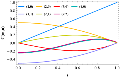
Figure 2: Cumulants $C(m,n)$ as a function of $t$ (transmission amplitude of the QPC) at zero temperature and for $\eta_{1}=1$, $\eta_{2}=-1$. The vertical axis is in arbitrary units and we set $V_{1}=V_{3}=e=h=1$.

3.2 Half-charge transfers

The cumulants $C(n,0)$ are obtained from the cumulant generating function

$$\ln\chi(\lambda)=\ln\left(1+P_{+}\left(e^{i\lambda}-1\right)+P_{-}\left(e^{-i\lambda}-1\right)\right)\>,$$ (19)

which follows from the full cumulant generating function (11) by summing over the outcomes in lead 4, and where $P_{\pm}=(1\pm\eta_{1}t)^{2}/4$ are the probabilities of transfering an electron or a hole into lead 2. Note that we still assume $T=0,\eta_{1,2}=\pm 1,V_{1}=V_{3}=V>0$.

We may add the side remark that the CGF in the case of $t=0$, viz. a simple Mach-Zehnder interferometer, corresponds to a trinomial process with equal probabilities $1/4$ for an electron to electron or to hole transfer process. This has been noted in [27], where the corresponding predictions for the conductance (it vanishes) and the noise (is quantized with a Fano factor 1/4) have been obtained. Recently a detailed analysis of the FCS has confirmed this prediction [34] and related it to the topological nature of the Majorana mode.

We are now ready to make the connection with the binomial process. Basically, it turns out that

$$\ln\chi(\lambda)= 2\ln\left(1+\frac{1+\eta_{1}t}{2}(e^{i\lambda/2}-1)+\frac{1-\eta_{1}t}{2}(e^{-i\lambda/2}-1)\right)\,.$$ (20)

This means that we can interpret unit-charge transfer processes as two independent half-charge transfer processes (notice the 2 multiplying the logarithm, and the factor $\lambda/2$ in the exponents). In other words, two independent binomial processes occuring with probability $p=(1+\eta_{1})/2$.

However, we do not expect physical half-charge transport processes because the existence of charge $e/2$ quasiparticles in this system is unlikely. We can also write Eq. (20) in the equivalent form

$$\ln\chi(\lambda)= i\lambda+2\ln\left(1+\frac{1-\eta_{1}t}{2}(e^{-i\lambda}-1)\right)\>,$$ (21)

which has a more mundane interpretation. Equation (21) represents two independent conversion processes: two incoming electrons can either go out as electrons with probability $\sqrt{P_{+}}$ each, or be converted to a hole with probability $\sqrt{P_{-}}$.

Both interpretations, with half-charges or with conversion processes, are deceptive. In reality, the two incoming electrons are not independent. However, the factorization of the process itself, regardless of its interpretation, is of special interest. This is a potential signature of Majorana fermions. We would like to point out that this factorization is only valid for a symmetric interferometer, or at zero bias. This could be potentially attributed to a special property of the $k=0$ Majorana mode (which is self-adjoint) that the $k\neq 0$ modes do not possess.

Similar half-charge full counting statistics have been found in other mesoscopic transport situations, e.g. a double-barrier structure (see Eq. (38) of [38] or Eq. (3.51) of [39]), or a voltage-driven quantum point contact strongly coupled to a charge qubit [40].

4 Factorization of transfer processes

To shed more light on this question, we will now study this factorization property for a general scattering matrix. As discussed before, in some circumstances, it is possible to factorize the charge transfer processes, such that the cumulant generating function takes the form

$$\ln\chi(\lambda_{2},\lambda_{4})=2\ln\chi^{\prime}(\lambda_{2},\lambda_{4})\>,$$ (22)

where the “half-CGF” $\ln\chi^{\prime}$ is expressed in terms of half-charge transfers

$$\ln\chi^{\prime}(\lambda_{2},\lambda_{4})=\ln\sum_{s_{2},s_{4}=-,0,+}P^{\prime}_{s_{2}s_{4}}e^{ie(s_{2}\lambda_{2}+s_{4}\lambda_{4})/2}\>.$$ (23)

Note the factor $1/2$ multiplying the counting fields in the exponent.

To see when this factorization is possible, let us compare $(\chi^{\prime})^{2}$ with $\chi$:

$$(\chi^{\prime})^{2}=\sum_{s_{2},s_{4},t_{2},t_{4}}P^{\prime}_{s_{2}s_{4}}P^{\prime}_{t_{2}t_{4}}e^{ie(\lambda_{2}(s_{2}+t_{2})/2+\lambda_{4}(s_{4}+t_{4})/2)}$$ (24)

The first conclusion we draw is that we cannot mix 0-charge transfers with $1/2$-charge transfers in $\chi^{\prime}$ in the same outgoing lead. Otherwise, we would still have $1/2$-charge transfers in $(\chi^{\prime})^{2}$. This means in Eq. (23) we must have either $s_{2,4}=\pm 1$ or $s_{2,4}=0$). The case of 0-charge transfer only is not interesting, so we focus on purely half-charge transfers. We obtain the following equations for the probabilities

$$(P^{\prime}_{\pm\pm})^{2} =P_{\pm\pm}\>,$$

$$(P^{\prime}_{\pm\mp})^{2} =P_{\pm\mp}\>,$$

$$2P^{\prime}_{\pm+}P^{\prime}_{\pm-} =P_{\pm 0}\>,$$

$$2P^{\prime}_{+\pm}P^{\prime}_{-\pm} =P_{0\pm}\>,$$

$$2P^{\prime}_{++}P^{\prime}_{--}+2P^{\prime}_{+-}P^{\prime}_{-+} =P_{00}\>.$$ (25)

The first two equations fully fix the four probabilities $P^{\prime}$, the three remaining equations are thus nontrivial conditions the probabilities $P$ must satisfy to make the factorization possible.

If we specialize to two-incoming-particle processes, we can refine the conditions on $P$. First, if we only have two-incoming-particle processes (this can be tuned by choosing proper occupations of the incoming leads, such as a symmetric bias and zero temperature), then $P_{\pm 0}=P_{0,\pm}=0$. The half-charge transfer process (i.e., the factorization) is then possible if either

$$\sqrt{P_{++}}+\sqrt{P_{--}}=1\quad{\rm or}\quad\sqrt{P_{+-}}+\sqrt{P_{-+}}=1\>.$$ (26)

Thus, we are really looking for a property of the scattering matrix (that is independent of the incoming leads’ occupation) rather than a property of the full counting statistics themselves. Typically, if two-particle processes and one-particle processes mix, we have no chance of finding such a factorization of the FCS.

We now specialize to the case where both electron incoming modes are fully occupied, and the hole modes fully unoccupied. This leads to the probabilities

$$\sqrt{P_{++}}=|s_{11}s_{33}-s_{13}s_{31}|\>,$$

$$\sqrt{P_{--}}=|s_{21}s_{43}-s_{23}s_{41}|\>,$$

$$\sqrt{P_{+-}}=|s_{11}s_{43}-s_{13}s_{41}|\>,$$

$$\sqrt{P_{-+}}=|s_{21}s_{33}-s_{23}s_{31}|\>.$$ (27)

Thus, checking the factorization property given in Eq. (26) has been reduced to a condition on the scattering matrix. The strategy will now be to investigate interferometers of increasing complexity by writing down their scattering matrices and checking whether Eq. (26) is fulfilled, i.e., whether the factorization property holds.

4.1 Double point-contact geometry

We first consider the double point-contact interferometer shown in Fig. 3a where the labels for the incoming and outgoing Majorana modes are defined.

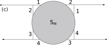
Figure 3: (a) Double point-contact geometry. (b) Central island geometry. (c) General scattering matrix. The numbers $1,2,3,4$ in the top-left and botton-right corners label the four incoming chiral Majorana modes, whereas the numbers in the top-right and bottom-left corners label the four outgoing Majorana modes. Incoming and outgoing Majorana modes are related by the scattering matrix $S_{M}$.

The conversion of Dirac to Majorana modes is achieved by [22]

$$S_{c}=\frac{1}{\sqrt{2}}\left(\begin{array}[]{cccc}\eta_{A}&\eta_{A}&0&0\\ i&-i&0&0\\ 0&0&-\eta_{C}&-\eta_{C}\\ 0&0&i&-i\end{array}\right)\>,$$ (32)

see A. Here $\eta_{A},\eta_{C}=\pm 1$ depend on the parity of the number of vortices. The minus sign in front of $\eta_{C}$ takes care of the $\pi$ Berry phase obtained when a Majorana fermion makes a $2\pi$ rotation. The back-conversion is similar,

$$S_{bc}=\frac{1}{\sqrt{2}}\left(\begin{array}[]{cccc}-i&\eta_{B}&0&0\\ i&\eta_{B}&0&0\\ 0&0&-i&\eta_{D}\\ 0&0&i&\eta_{D}\end{array}\right)\>,$$ (37)

The tunneling of Majorana fermions is described by the $SO(4)$ matrix

$$S_{M}=\left(\begin{array}[]{cccc}0&-t&0&r\\ r^{\prime}&0&t^{\prime}&0\\ 0&r&0&t\\ -t^{\prime}&0&r^{\prime}&0\end{array}\right)\>.$$ (42)

The total scattering matrix is given by the product of these three scattering matrices

$$S =S_{bc}S_{M}S_{c}$$ (43)

which is real. Using Eq. (27), one obtains

$$\sqrt{P_{++}}+\sqrt{P_{--}}=\frac{1+\eta}{2}\>,$$ (44)

$$\sqrt{P_{+-}}+\sqrt{P_{-+}}=\frac{1-\eta}{2}\>,$$ (45)

i.e., the sums of the probability amplitudes are seen to fulfill Eq. (26). Thus, factorization holds, and the two-incoming-electron processes can be written as two equal and independent processes.

4.2 Central Majorana island geometry

We define the matrix

$$X=\left(\begin{array}[]{cccc}0&0&0&1\\ 1&0&0&0\\ 0&1&0&0\\ 0&0&1&0\end{array}\right)\>,$$ (50)

as well as $R=\mathrm{diag}(r_{1},r_{2},r_{3},r_{4})$, and $T=\mathrm{diag}(t_{1},t_{2},t_{3},t_{4})$. Using $(XR)^{4}=r_{1}r_{2}r_{3}r_{4}\equiv r$ is proportional to the identity matrix, we find

$$S_{M}=XR-\frac{1}{1-r}XT(1+XR+(XR)^{2}+(XR)^{3})XT\>.$$ (51)

The relevant matrix elements of the total scattering matrix $S=S_{bc}S_{M}S_{c}$ read

$$s_{11} =\frac{1}{2}\left(r_{1}-\frac{t_{1}r_{2}r_{3}r_{4}t_{1}+t_{4}r_{1}t_{2}-i(t_{4}t_{1}-t_{1}t_{2})}{1-r}\right)\>,$$

$$s_{33} =\frac{1}{2}\left(r_{3}-\frac{t_{3}r_{4}r_{1}r_{2}t_{3}+t_{2}r_{3}t_{4}-i(t_{2}t_{3}-t_{3}t_{4})}{1-r}\right)\>,$$

$$s_{13} =\frac{1}{2}\left(r_{4}-\frac{t_{4}r_{1}r_{2}r_{3}t_{4}+t_{1}r_{2}t_{3}-i(t_{4}r_{1}r_{2}t_{3}-t_{1}r_{2}r_{3}t_{4})}{1-r}\right)\>,$$

$$s_{31} =\frac{1}{2}\left(r_{2}-\frac{t_{2}r_{3}r_{4}r_{1}t_{2}+t_{3}r_{4}t_{1}-i(t_{2}r_{3}r_{4}t_{1}-t_{3}r_{4}r_{1}t_{2})}{1-r}\right)\>,$$

$$s_{21} =\frac{1}{2}\left(r_{1}-\frac{t_{1}r_{2}r_{3}r_{4}t_{1}-t_{4}r_{1}t_{2}+i(t_{4}t_{1}+t_{1}t_{2})}{1-r}\right)\>,$$

$$s_{43} =\frac{1}{2}\left(r_{3}-\frac{t_{3}r_{4}r_{1}r_{2}t_{3}-t_{2}r_{3}t_{4}+i(t_{2}t_{3}+t_{3}t_{4})}{1-r}\right)\>,$$

$$s_{23} =\frac{1}{2}\left(-r_{4}-\frac{-t_{4}r_{1}r_{2}r_{3}t_{4}+t_{1}r_{2}t_{3}+i(t_{4}r_{1}r_{2}t_{3}+t_{1}r_{2}r_{3}t_{4})}{1-r}\right)\>,$$

$$s_{41} =\frac{1}{2}\left(-r_{2}-\frac{-t_{2}r_{3}r_{4}r_{1}t_{2}+t_{3}r_{4}t_{1}+i(t_{2}r_{3}r_{4}t_{1}+t_{3}r_{4}r_{1}t_{2})}{1-r}\right)\>.$$ (52)

If only one QPC has a non-vanishing transmission, the scattering matrix reduces to the HBT case. For $t_{2}\equiv t$, $t_{4}=1$, and $t_{1}=t_{3}=0$, we get back the setup HBT with one QPC. For the case where all QPC are equal, $t_{i}\equiv t$, the factorization also holds. The same is true for $t_{1}=t_{4}\equiv t$ and $t_{2}=t_{3}=0$ although this situation is less symmetric.

We were unable to prove the factorization property for general values $t_{i}$ analytically. We therefore used a numerical approach: in the spirit of a Monte-Carlo calculation, we generated many scattering matrices by using random values of the transmission amplitudes $t_{i}$. The factorization was then confirmed by checking that $\sqrt{P_{++}}+\sqrt{P_{--}}=|s_{11}s_{33}-s_{13}s_{31}|+|s_{21}s_{43}-s_{23}s_{41}|=0\quad\mathrm{or}\quad 1$. This is indeed the case, i.e., the factorization property holds for the island geometry as well.

4.3 Most general scattering matrix

We now consider the most general case: a general $SO(4)$ matrix accompanied by the appropriate Dirac to Majorana conversion / back-conversion, see Fig. 3c. The conversion from Dirac to Majorana channels reads

$$S_{c}=\frac{1}{\sqrt{2}}\left(\begin{array}[]{cccc}1&1&0&0\\ i&-i&0&0\\ 0&0&-1&-1\\ 0&0&i&-i\end{array}\right)\>;$$ (57)

the back-conversion is similar

$$S_{bc}=\frac{1}{\sqrt{2}}\left(\begin{array}[]{cccc}-i&1&0&0\\ i&1&0&0\\ 0&0&-i&1\\ 0&0&i&1\end{array}\right)\>.$$ (62)

The total scattering matrix is

$$S=S_{bc}S_{M}S_{c}\>,$$ (63)

where $S_{M}\in SO(4)$. Again, we demonstrated the factorization property numerically by generating a set of random $SO(4)$ matrices and constructing the corresponding scattering matrix $S$ defined by Eq. (63). The factorization property (26) was found to hold even in this most general case.

4.4 More than four terminals

Finally, let us discuss how the peculiar properties of the CGF can be generalized to setups with more than four terminals. In the case of six terminals, for instance, a general scattering matrix between incoming and outgoing Dirac fermions can be expressed as

$$S=S_{bc}S_{M}S_{c}\>,$$ (64)

where $S_{M}$ is a general $SO(6)$ matrix, and $S_{c}$ and $S_{bc}$ denote the $6\times 6$ conversion and back-conversion matrices. If particles enter via the leads $1,3,5$ and exit via the leads $2,4,6$, then the most general CGF is a generalization of Eq. (11),

$$\chi(\lambda_{2},\lambda_{4},\lambda_{6})=\sum_{s_{2},s_{4},s_{6}=-,0,+}P_{s_{2}s_{4}s_{6}}e^{i(s_{2}\lambda_{2}+s_{4}\lambda_{4}+s_{6}\lambda_{6})}\>.$$ (65)

If we focus again on the limit of equal positive bias voltages $V_{1}=V_{3}=V_{5}>0$, then all incoming electron modes are occupied and all incoming hole modes are empty. In that case, in analogy to Eq. (27), one finds, e.g., for the probability $P_{+++}$ of finding particles in all outgoing modes and the probability $P_{++-}$ to find particles exiting in leads $2$ and $4$ and a hole exiting via lead 6,

$$\sqrt{P_{+++}} =\sum_{\mathcal{P}\in S_{135}}|(-1)^{\text{sgn}(\mathcal{P})}s_{1,\mathcal{P}1}s_{3,\mathcal{P}3}s_{5,\mathcal{P}5}|,$$

$$\sqrt{P_{++-}} =\sum_{\mathcal{P}\in S_{136}}|(-1)^{\text{sgn}(\mathcal{P})}s_{1,\mathcal{P}1}s_{3,\mathcal{P}3}s_{5,\mathcal{P}6}|.$$ (66)

where the summation is over the six permutations of the respective set. With our choice of phases in the conversion matrices, one finds that for an arbitrary $SO(6)$ matrix $S_{M}$ only processes with outgoing charge $3$ and $-1$ have a nonzero probability,

$$P_{+++}+P_{+--}+P_{-+-}+P_{--+} =1,$$

$$P_{++-}=P_{+-+}=P_{-++}=P_{---} =0.$$ (67)

Using the first line to eliminate $P_{+++}$, one finds that the CGF is given by a generalization of Eq. (21),

$$\ln\chi(\lambda_{2},\lambda_{4},\lambda_{6})=i(\lambda_{2}+\lambda_{4}+\lambda_{6})+\ln\bigg{[}1+P_{+--}(e^{-2i(\lambda_{4}+\lambda_{6})}-1)$$

$$+ P_{-+-}(e^{-2i(\lambda_{2}+\lambda_{6})}-1)+P_{--+}(e^{-2i(\lambda_{2}+\lambda_{4})}-1)\bigg{]}$$ (68)

Evidently, for a general scattering matrix the six-terminal result contains more free parameters than the four-terminal case. This means that it is no longer possible to factorize the FCS in general.

However, one still finds that only a very limited number of scattering processes are possible: either two of the incoming eletrons are transmitted as holes (with probabilities $P_{+--}$, $P_{-+-}$ and $P_{--+}$) or all electrons are transmitted as electrons.

5 Discussion/Conclusion

To summarize, we have calculated and analyzed the full counting statistics of a modified Hanbury Brown-Twiss interferometer for chiral Majorana fermions which contain information about higher-order current correlation and generalize the results presented in [27]. Most of the calculations in this paper are valid only at zero energy, at which particle-hole symmetry enforces important constraints on the scattering matrices. Some of the obtained results are expected to remain valid at finite, but low, energies. However, we also do not keep track of dynamical phases which are important even at low energies.

The full counting statistics calculated in this paper exhibit an interesting factorization property that points towards the interpretation of a unit-charge transfer process as two independent half-charge transfer processes. We checked the factorization property for increasingly more general scattering matrices and confirmed numerically that it holds for the most general $SO(4)$ matrix at specific configurations of voltage bias and at zero temperature. It is tantalizing to interpret this property as a signature of Majorana fermions, however, since we do not expect physical 1/2 charges to be transferred, its interpretation remains open at present.

6 Acknowledgment

GS and CB acknowledge financial support by the the Swiss SNF and the NCCR Quantum Science and Technology. WB was financially supported by the DFG through SFB 767 and BE 3803/5-1. TLS acknowledges support by National Research Fund, Luxembourg (ATTRACT 7556175).

Appendix A Majorana interferometers basics

In this appendix, we list some of the basic building blocks needed to study concrete interferometric structures, compute their scattering matrix, and check whether the FCS factorization holds.

A.1 Dirac to Majorana converter

This is the building block to connect Majorana fermions to external Dirac fermions [22, 25]. The scattering matrix that relates chiral Dirac fermions to chiral Majorana fermions at T-junctions is fully determined by particle-hole symmetry and unitarity. Its form is given by

$$S_{\mathrm{conv}}=\frac{1}{\sqrt{2}}\left(\begin{array}[]{cc}1&1\\ i&-i\end{array}\right)\>,$$ (71)

such that

$$\left(\begin{array}[]{c}\gamma_{1}\\ \gamma_{2}\end{array}\right)=S_{\mathrm{conv}}\left(\begin{array}[]{c}\psi_{e}\\ \psi_{h}\end{array}\right)\>.$$ (76)

The only remaining freedom is a physically unimportant phase factor that corresponds to gauge transformations

$$S_{\mathrm{conv}}\longrightarrow S_{\mathrm{conv}}\left(\begin{array}[]{cc}e^{i\alpha}&0\\ 0&e^{-i\alpha}\end{array}\right)\>.$$ (79)

As long as the Dirac fermions in the external channels do not interfere with one another, these factors are irrelevant.

The back conversion of Majorana to Dirac fermions is described by the time-reversed scattering matrix

$$S_{\mathrm{back-conv}}=\frac{1}{\sqrt{2}}\left(\begin{array}[]{cc}1&i\\ 1&-i\end{array}\right)\>.$$ (82)

A.2 Majorana fermion point contact

Because of particle-hole symmetry, the scattering matrix that relates chiral Majorana fermions before and after a quantum point contact (QPC), or any form of tunneling, must be real. The scattering matrix is therefore a rotation matrix that can be parametrized by a single angle. We use $r,t$ as the (real) reflection and transmission amplitudes of the point contacts to write

$$\left(\begin{array}[]{c}\gamma_{1}^{\prime}\\ \gamma_{2}^{\prime}\end{array}\right)=\left(\begin{array}[]{cc}r&t\\ -t&r\end{array}\right)\left(\begin{array}[]{c}\gamma_{1}\\ \gamma_{2}\end{array}\right)\>.$$ (89)

Note that tunneling between a pair of Majorana channels directly after the conversion from Dirac fermions can be described by the product of two scattering matrices

$$S_{\mathrm{tot}}=S_{\mathrm{tunnel}}S_{\mathrm{conv}} =\frac{1}{\sqrt{2}}\left(\begin{array}[]{cc}r+it&r-it\\ -t+ir&-t-ir\end{array}\right)$$ (92)

$$=\frac{1}{\sqrt{2}}\left(\begin{array}[]{cc}e^{i\alpha}&e^{-i\alpha}\\ ie^{i\alpha}&-ie^{-i\alpha}\end{array}\right)\>,$$ (95)

where we defined $r+it=e^{i\alpha}$. We can write this as

$$S_{\mathrm{tot}}=S_{\mathrm{conv}}\left(\begin{array}[]{cc}e^{i\alpha}&0\\ 0&e^{-i\alpha}\end{array}\right)\>.$$ (98)

The effect of tunneling is therefore equivalent to a redefinition of the phases of the incoming Dirac modes and can be disregarded.

References

- [1] M. Büttiker, Phys. Rev. Lett. 68, 843 (1992).
- [2] V.A. Khlus, Sov. Phys. JETP 66, 1243 (1987).
- [3] G.B. Lesovik, Pis’ma Zh. Eksp. Teor. Fiz. 49, 515 (1989) [JETP Lett. 49, 594 (1989)].
- [4] M. Büttiker, Phys. Rev. Lett. 65, 2901 (1990).
- [5] T. Martin and R. Landauer, Phys. Rev. B 45, 1742 (1992).
- [6] M. Büttiker, Phys. Rev. B 46, 12485 (1992).
- [7] T. Martin, Phys. Lett. A 220, 137 (1996)
- [8] M.P. Anantram and S. Datta, Phys. Rev. B 53, 16390 (1996).
- [9] J. Börlin, W. Belzig, and C. Bruder, Phys. Rev. Lett. 88, 197001 (2002).
- [10] P. Samuelsson and M. Büttiker, Phys. Rev. Lett. 89, 046601 (2002).
- [11] A. Cottet, W. Belzig, and C. Bruder, Phys. Rev. Lett. 92, 206981 (2004).
- [12] A. Cottet and W. Belzig, Europhys. Lett. 66, 405 (2004).
- [13] W. Belzig, Phys. Rev. B 71, 161301(R) (2005).
- [14] A.Y. Kitaev, Physics-Uspekhi 44, 131 (2001).
- [15] D.A. Ivanov, Phys. Rev. Lett. 86, 268 (2001).
- [16] C. Nayak, S.H. Simon, A. Stern, M. Freedman, and S. Das Sarma, Rev. Mod. Phys. 80, 1083 (2008).
- [17] J. Alicea, Y. Oreg, G. Refael, F. von Oppen, and M.P.A. Fisher, Nature Phys. 7, 412 (2010).
- [18] A. Stern and N.H. Lindner, Science 339, 1179 (2013).
- [19] V. Mourik et al., Science 336, 1003 (2012).
- [20] A. Das, Y. Ronen, Y. Most, Y. Oreg, M. Heiblum, and H. Shtrikman, Nature Phys. 8, 887 (2012).
- [21] L.P. Rokhinson, X. Liu, and J.K. Furdyna, Nature Phys. 8, 795 (2012).
- [22] A.R. Akhmerov, J. Nilsson, and C.W.J. Beenakker, Phys. Rev. Lett. 102, 216404 (2009).
- [23] J. Nilsson and A.R. Akhmerov, Phys. Rev. B 81, 205110 (2010).
- [24] E. Grosfeld and A. Stern, PNAS 108, 11810 (2010).
- [25] L. Fu and C.L. Kane, Phys. Rev. Lett. 102, 216403 (2009).
- [26] C.-X. Liu and B. Trauzettel, Phys. Rev. B 83, 220510 (2011).
- [27] G. Strübi, W. Belzig, M.-S. Choi, and C. Bruder, Phys. Rev. Lett. 107, 136403 (2011).
- [28] S. Bose and P. Sodano, New J. Phys. 13, 085002 (2011).
- [29] Jian Li, G. Fleury, and M. Büttiker, Phys. Rev. B 85, 125440 (2012).
- [30] L.S. Levitov and G.B. Lesovik, JETP Lett. 58, 230 (1993).
- [31] B.A. Muzykantskii and D.E. Khmelnitskii, Phys. Rev. B 50, 3982 (1994).
- [32] W. Belzig and Yu.V. Nazarov, Phys. Rev. Lett. 87, 197006 (2001).
- [33] G. Strübi, Thesis, University of Basel (2014).
- [34] N.V. Gnezdilov, B. van Heck, M. Diez, J.A. Hutasoit, and C.W.J. Beenakker, arXiv:1505.06744
- [35] L. Weithofer, P. Recher, and T.L. Schmidt, Phys. Rev. B 90, 205416 (2014).
- [36] P. Samuelsson, E.V. Sukhorukov, and M. Büttiker, Phys. Rev. Lett. 92, 026805 (2004).
- [37] I. Klich, in Quantum Noise, edited by Yu.V. Nazarov and Ya. M. Blanter (Kluwer 2003). arXiv:cond-mat/0209642 (2002).
- [38] M.J.M. de Jong, Phys. Rev. B 54, 8144 (1996).
- [39] Y.V. Nazarov and Y.M. Blanter, Quantum Transport (Cambridge University Press, Cambridge, 2009).
- [40] I. Snyman and Y.V. Nazarov, Phys. Rev. Lett. 99, 096802 (2007).