Large-angle scattering of multi-GeV muons on thin Lead targets

Abstract

The probability of large-angle scattering for multi-GeV muons in thin lead targets ($t/X_{0}$ of ${\mathcal{O}}(10^{-1})$) is studied. The new estimates presented here are based both on simulation programs (GEANT4 libraries) and theoretical calculations. In order to validate the results provided by simulation, a comparison is drawn with experimental data from the literature. This study is particularly relevant when applied to muons originating from $\nu_{\mu}$ CC interactions of CNGS beam neutrinos. In that circumstance the process under study represents the main background for the $\nu_{\mu}\to\nu_{\tau}$ search in the $\tau\to\mu$ channel for the OPERA experiment at LNGS. Finally we also investigate, in the CNGS context, possible contributions from the muon photo-nuclear process which might in principle also produce a large-angle muon scattering signature in the detector.

I Introduction

Multiple Coulomb scattering has been studied extensively in the past in many different conditions and for different incident particles both theoretically and experimentally. In this work we are interested in the characterisation of large-angle Multiple Coulomb Scattering (LAS) of multi-GeV muons scattering over high-$Z$ materials with a thickness being a fraction of the radiation length $X_{0}$ (i.e. thickness ${\mathcal{O}}$(1 mm)). In the LAS regime we are interested in, the transferred momentum $q$ is such that the De Broglie wavelength ($\lambda\simeq\hbar/q$) of the probe is much smaller ($<1$ fm) than the typical radial extension of a high-$Z$ nucleus (about 6-7 fm for Lead). For a correct description of the high-angle tails of the scattering angle distribution it is thus mandatory to precisely take into account the effect of the nuclear charge distribution as well as the contribution of scattering off individual protons.

In Sect. II we review basic theoretical aspects of the problem highlighting the associated challenges. In Sect. III we overview the available approaches for simulating multiple Coulomb scattering while in Sect. IV we describe specifically the simulation program developed for this work using GEANT4 ([1], [2]) libraries. In Sect. V we compare the developed simulation with a theoretical approach described in Sect. II. In Sect. VI we validate the simulation on experimental data coming from past experiments designed to study the nuclear charge density. Finally, in Sect. VII, the impact of LAS as a background for the $\nu_{\mu}\to\nu_{\tau}$ search is evaluated. The importance of muon photo-nuclear interactions in mimicking LAS topologies at CNGS is evaluated in Sect. VIII.

II Multiple scattering theories

Multiple scattering has been an active field of theoretical and experimental efforts since very early days of particle physics. Goudmit-Saunderson [3, 4] and Lewis [5] developed a theory which allows to calculate the exact distribution of the angle in space ($\theta$) due to multiple scattering after a given path $s$. The problem was tackled by formulating it in terms of a transport equation solved by expanding the angular dependence in Legendre polinomials ($P_{l}(\cos\theta)$). The angular distribution is found to be given by:

$$F(\theta,s)=\sum_{l=0}^{\infty}\frac{2l+1}{4\pi}e^{-{\frac{s}{\lambda_{l}}}}P_{l}(\cos\theta)$$ (1)

with the transport mean free paths defined as:

$${\lambda_{l}}^{-1}=e^{-2\pi sN\int_{-1}^{1}{(1-P_{l}(\cos x))\frac{d\sigma(x)}{d\Omega}}d(\cos x)}.$$ (2)

The theory does not assume any particular form of the single scattering differential cross section $d\sigma/d\Omega$ and provides exact solutions. It can also deal with arbitrary nuclear form factors provided that integrals are evaluated numerically. Nevertheless for large scattering angles the calculation requires the evaluation of high order Legendre polinomials which are difficult to treat. This limitation is also relevant for the present case and hence this approach was not considered further.

Another interesting theoretical study was performed in [6] by Meyer. The theory by Molière [7, 8] is there extended to take into account a generic nuclear form factor. The general distribution of the scattering angle $\theta$ is derived and, for a point-like nucleus, it reads as:

$$F(\theta,t)\theta d\theta=2\chi e^{-\chi^{2}}\left[1+\frac{b_{0}+b_{2}\chi^{2}+\sum_{\nu=2}^{\infty}{b_{2\nu}\chi^{2\nu}}}{B}\right]d\chi$$ (3)

$\chi$ being equal to $\theta$ apart for numerical constants which depend on the parameters of the problem (incoming momentum, particle, target thickness, density etc.) which are made explicit in Appendix A. The other quantities are either constants $b_{0}=0.423$, $b_{2}=-1.423$, $b_{2\nu}=\frac{(\nu-2)!}{(\nu!)^{2}}$ or simple functions of the system parameters as for $B$ (see Appendix A for more details). The component having the form $\chi e^{-\chi^{2}}$ results from multiple consecutive scattering in the target thickness while the tail at higher $\chi$ arises from the occurrence of single high angle scattering. For a finite nucleus with a charge density distribution $q(x)$ the $b_{0,2,2\nu}$ coefficients in Eq. 3 are replaced by other coefficients $c_{0,2,2\nu}$ involving integrals of the form factor $q(x)$ (see Appendix A). If we approximate the charge density of the nucleus as a uniform sphere the resulting form factor takes this form:

$$q(x)=\frac{9}{x}\left[\frac{\sin{x}}{x}-\cos x\right]$$ (4)

As a further simplification we can approximate $q(x)$ with a Gaussian function $q=e^{-ax^{2}}$. The coefficients $c_{0,2,2\nu}$ can then be expressed analitically as simple functions of $Z$, $a$ and the nuclear radius (Appendix A). Unfortunately also this method faces numerical limitations that we will discuss in Sect. V. It will anyway be used for small scattering angles as a validation for the Monte Carlo approach which we are about to describe in Sect. III.

III Monte Carlo simulation of multiple scattering

Multiple Coulomb scattering can be simulated numerically using different approaches:

• detailed simulations: each track is simulated at microscopic level as a succession of connected straight segments (free-flights), Changes of direction are determined by sampling the polar deflection $\cos\theta$ from the single scattering distribution, and the azimuthal scattering angle uniformly in [0, 2$\pi$]. The length $t$ of the free-flight is sampled from the exponential distribution $p(t)=\lambda^{-1}e^{-t/\lambda}$. The simulated angular and spatial displacements are “exact”, i.e. they coincide with those obtained from a rigorous solution of the problem (i.e. by mean of the transport equation introduced in the theories of Goudsmit-Saudersons [3, 4] and Lewis [5]). Nevertheless detailed simulations are in practice not possible computationally except for specific cases involving very low energies and thicknesses.

• condensed simulations: the global effects of the collisions during a macroscopic step are simulated using approximations. Usually the theories of Goudsmit-Saundersons [3, 4], Molière [7, 8] and Lewis [5] are used to predict the angular and spatial distributions after each step. At energies where condensed algorithms are required, the great majority of elastic collisions are “soft” collisions with very small deflections. Especially the spatial distributions might present significant dependencies on the choice of the macroscopic step which has to be carefully studied.

• mixed algorithms: Hard collisions, with scattering angle $\theta$ larger than a given value $\theta_{S}$, are individually simulated and soft collisions (with $\theta<\theta_{S}$) are described by means of a multiple scattering approach. It is clear that, by selecting a conveniently large value for the cutoff angle $\theta_{S}$, the number of hard collisions per electron track can be made small enough to allow their detailed simulation. The value of the mean free path between the simulation of hard collisions, $\lambda_{(h)}$, is given by $\lambda_{(h)}^{-1}=2\pi N\int_{\theta_{S}}^{\pi}\sigma(\theta)\sin\theta d\theta$. As the fluctuations in the spatial displacement after a certain path length are mainly due to hard collisions, a mixed procedure (with a suitably small value of $\theta_{S}$) yields spatial and angular distributions that are more accurate than those from a condensed simulation.

Since we are interested in rare high-$q$ events a mixed algorithm approach has been preferred. Furthermore in this scheme the inclusion of nuclear effects can be easily taken into account when sampling the angular distribution at single-scattering level.

IV The Geant4 Monte Carlo implementation

The version of Geant4 used for this study is 4.9.6.p02 with the standardSS physics list option to enable the treatment of single scattering above a certain angular threshold. The simulation of single-scattering is dealt with by the routine G4WentzelOKandVIxSection.cc. The distribution of the step length used by the GEANT4 simulation is shown in Fig. 1 for 2 GeV/c muons on 1 mm thick lead target. The slope of the exponential distribution corresponds to a value of $\lambda_{(h)}=0.14~{}\mu$m such that the single-scattering code is invoked on average about 7000 times for each muon crossing the 1mm thick lead target.

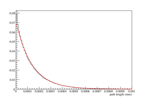
Figure 1: Distribution of the step length for the GEANT4 mixed simulation for 2 GeV/c muons over 1 mm of Lead.

The event sampling is done according to the model by Wentzel [9] in the formulation of [10]. The model adopts a modified Coulomb potential to take into account the effect of the screening of the electron cloud: $V(r)=(Ze^{2}/r)e^{-r/R}$. A slightly modified version of the Molière screening angle $\chi_{a}^{\prime}=(\frac{\hbar}{2pR})^{2}$ is used whose $Z$ and energy dependence is parametrised as (cfr. [10], eq. 23):

$$\chi_{a}^{\prime}=\frac{\alpha^{2}{a_{0}^{2}Z^{2/3}}}{p^{2}}\left(1.13+3.76\left(\frac{\alpha Z}{\beta}\right)^{2}\sqrt{\frac{\tau}{\tau+Z^{2/3}}}\right)$$ (5)

$a_{0}$ being the Bohr radius and $\tau=E_{kin}/m$.

If we define $\mu=\frac{1}{2}(1-\cos\theta)$ the differential cross section $d\sigma/d\mu$ in presence of screening is proportional to $\sim p^{-2}(\chi_{a}^{\prime}+\mu)^{-2}$. The inverse transform method leads to the following sampling formula:

$$\mu=\mu_{S}+\frac{(\chi_{a}^{\prime}+\mu_{S})\zeta(1-\mu_{S})}{(\chi_{a}^{\prime}+1)-\zeta(1-\mu_{S})}\simeq\frac{\mu_{S}}{1-\zeta(1-\mu_{S})}$$ (6)

with $\mu_{S}=\frac{1}{2}(1-\cos\theta_{S})$. In the multi-GeV regime the screening parameter $\chi_{a}^{\prime}$ is found to be of ${\mathcal{O}}(10^{-12})$ and hence the sampled distribution effectively reduces to a Rutherford law $dN/d\theta\propto(1-\cos\theta)^{-2}$. The single scattering angular distribution generated from Eq.6 is then corrected for effects related to the atomic electrons, the nuclear recoil and the nuclear charge density by introducing a function $g_{rej}(\theta)=g_{a}(\theta)\times g_{rec}(\theta)\times|F_{N}(\theta)|^{2}$. A random number $\zeta^{\prime}$ is thrown between 0 and 1 and the scattering is discarded if $\zeta^{\prime}>g_{rej}$. The atomic correction reads $g_{a}(\theta)=1-\beta^{2}\sin^{2}\frac{\theta}{2}+\frac{\alpha\beta\pi Z}{2}(1+\cos\theta)\sin{\frac{\theta}{2}}$ while the recoil correction follows the term found in the Mott scattering formula $g_{rec}=\left(1+(1-\cos\theta)\frac{p}{M}\right)^{-1}$.

In the standard implementation nuclear charge effects are implemented through a dipole form factor $|F_{N}(q)|^{2}={(1+\frac{1}{12}(\frac{qR_{N}}{197})^{2})}^{-2}$ with $q\simeq p\theta$ in MeV. The nuclear extension is parametrised as $R_{N}=1.27A^{0.27}$ giving $R_{N}=5.37$ fm for the ²⁰⁸Pb nucleus. Dipole form factors arise from an exponentially decreasing nuclear charge density and are thus not appropriate to describe the charge distribution of large nuclei. We have then modified the simulation program by introducing an ad hoc form factor for Lead based on the Saxon-Woods parametrisation of the charge density which is known to produce a much more realistic description:

$$\rho_{SW}(r)=\rho_{0}\left(1+e^{\frac{r-b}{a}}\right)^{-1}$$ (7)

The Saxon-Woods form factor has been fitted on precise electron scattering data available in the literature [11]. We have used $b=6.647$ fm and $a=2.30/(4\ln 3)$ fm as in [12]. The dipole form factor predicts a largely overestimated contribution of high-$q$ scatterings due to the assumption of a charge density being much more concentrated with respect to what is actually observed. It is hence only appropriate for small $q$. The form factor $|F_{N}^{SW}(q)|^{2}$ has been then extracted numerically by taking the squared Fourier transformation of the charge density $\rho_{SW}(r)$. The analytical dipole formula for $|F_{N}(q)|^{2}$ has been then replaced by a look-up table representing the Saxon-Wood form-factor of in bins of $q$ (100 bins from $q=0$ to $q=788$ MeV/c). Values above 788 MeV have been neglected. We have also considered the contribution of scattering on single protons ($F_{p}$) by composing the two effects according to the relative charge $Z$ following the procedure of Butkevic et al. ([13]):

$$|F(q)|^{2}=|F_{N}^{SW}(q)|^{2}+\frac{1}{Z}(1-|F_{N}^{SW}(q)|^{2})|F_{p}(q)|^{2}$$ (8)

Equation 8 is the same as Eq. 4 of ([13]) neglecting the atomic form factor which is only relevant at very small momentum transfer. For the proton form factor $F_{p}$ we have used an exponential charge density (dipole) with $\rho(r)=R_{p}^{-1}e^{-\frac{r}{R_{p}}}$ and $R_{p}=0.71$ fm.

The Lead form factor $|F_{N}^{SW}(q)|^{2}$ used in the simulation is shown in Fig. 2 (solid curve). The inclusion of scattering off protons (dotted curve) increases significanlty the probability of large-angle scattering as shown in Fig. 2, bottom, as it can be seen by comparing the solid ($|F(q)|^{2}$) and dotted ($|F_{N}(q)|^{2}$) curved. In summary the sampling is applied using a $g_{rej}^{\prime}(\theta)=g_{rec}(\theta)\times|F(q)|^{2}\times g_{a}(\theta)$. At the interesting energies the effect of atomic corrections is essentially absent ($g_{a}>1$ for any angle) and recoil introduces a modest correction due to $p/M$ being $\simeq 0.5-7\%$.

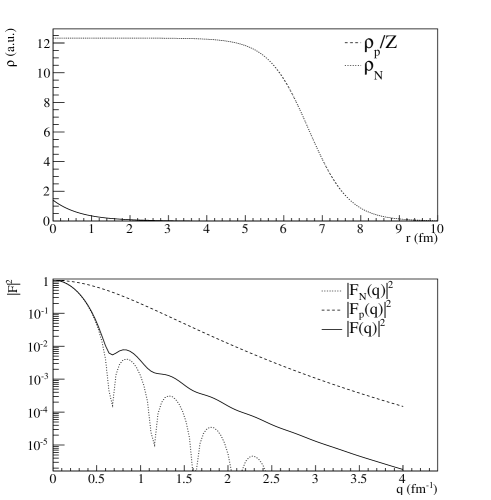
Figure 2: Top: charge density for the Lead nucleus according to the Saxon-Woods parametrization of Eq. 7 with the parameters described in the text (dotted line) and for the proton (continuous line). The relative size is given by $Z=82$. Bottom: the nuclear form factor obtained by the squared Fourier transform of $\rho_{SW}(r)$ ($|F_{N}(q)|^{2}$, dotted), the proton form factor obtained by the squared Fourier transform of $\rho_{p}(r)$ ($|F_{p}(q)|^{2}$, dashed). The combined form factor ($|F(q)|^{2}$, continuous) as in Eq. 8.

V Benchmarking the Monte Carlo with theoretical predictions

We have compared the result of the Monte Carlo simulation of Sect. IV for muons of 2, 8 and 14 GeV/c momenta and orthogonal incidence on a 1 mm thick Lead foil with the predictions of the theory by Meyer discussed in Sect. II. The results are shown in Fig. 3 (2 GeV/c), Fig. 4 (8 GeV/c) and Fig. 5 (14 GeV/c). The Monte Carlo distribution is shown by the histogram while theoretical predictions are shown by the dashed curves. Both the expectation for a point-like (red) or diffuse (black) charge distribution are shown. It can be noticed that the theoretical predictions show a steep drop above a certain value which depends on the muon momentum. This is understood in terms of numerical accuracy of the program (the sums in Eqns. 15 and 18 involve terms with large powers of $\theta$). This behaviour prevents using the Meyer theory for a quantitative estimate of LAS, as anticipated. Nevertheless we note that, despite the approximations used in deriving the theoretical curves (Sect. II), below the critical maximal angle, there is a resonable agreement with the Monte Carlo results.

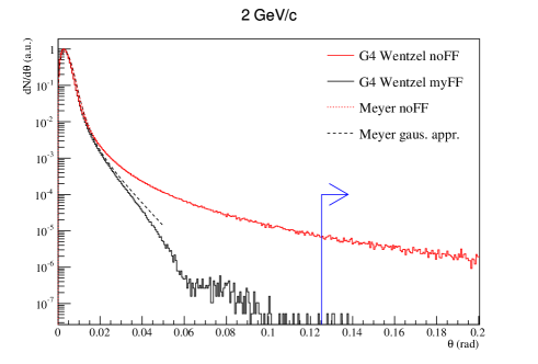
Figure 3: Distribution of the scattering angle for 2 GeV/c muons impinging orthogonally on a 1 mm thick lead target according to the prediction from the theory of Meyer (lines) and to the GEANT4 based simulation described in the text (histograms). Both the cases of a point-like or extended nucleus are shown in red and black respectively. The arrow marks the angle corresponding to the OPERA signal region (Sect.VII).

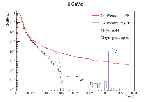
Figure 4: As for Fig. 3 but for 8 GeV/c muons.

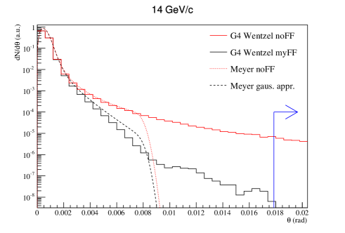
Figure 5: As for Fig. 3 but for 14 GeV/c muons.

VI Benchmarking the Monte Carlo with experimental data

We have tested the capability of the modified Monte Carlo (Sect. IV) to reproduce several data-sets available in the literature. The goal of these experiments was to investigate the scattering of muons or electrons at high momentum transfer to study the nuclear charge distribution. They are hence particularly suited for our purpose despite being rather old. A certain degree of extrapolation is present with respect to the CNGS case due to the use of different energy and particles and targets. This is mitigated by the fact that a significant variation of these parameters is sampled and that overall the conditions are not too dissimilar to the case of interest. A summary of the basic parameters of the used data-set is given in Tab. I.

$p$ (GeV/c)	particle	material	$t$ (mm)	$n_{data}$	Ref.
7.3	$\mu$	Cu	14.4	$3.1\times 10^{4}$	[14]
11.7	$\mu$	Cu	14.4	$8.7\times 10^{3}$	[14]
2.0	$\mu$	Pb	12.6	$2.5\times 10^{7}$	[15]
0.512	$e$	Pb	0.217	$\sim(1.25\times 10^{14})/\rm{s}$	[11]
$[$1, 15$]$	$\mu$	Pb	2.0	${\mathcal{O}}(10^{4})$	[16], [17]

TABLE I: Experimental data-sets used for the benchmarking of the simulation. $n_{data}$ indicates the number of measured particles.

The Copper targets are about a factor 3-4 thicker than the OPERA case while the momentum is in the OPERA window. The Lead data are represented by a target being thinner by about a factor ten (low-momentum electrons) and one being about a factor five thicker but in the OPERA momentum window. It must be noted that however the characteristic quantity of the process is the transverse momentum transfer $q$ rather than the incident momentum. The ability of the simulation in describing the data in this space is a good indicator of its reliability in the OPERA region of interest.

VI-A Copper data with muons (Akimenko et al.)

The experiment [14] was performed in 1986 at the IHEP accelerator using the HYPERON setup to measure the scattering of muons of energies of 7.3 and 11.7 GeV/c off a 14.4 mm thick (one $X_{0}$) Copper target. The incoming muon direction was determined with four proportional chambers allowing a spatial resolution of 0.7 mm and an angular accuracy of 0.3 mrad. A magnet was also employed allowing the incoming momentum to be estimated with a 3% relative error. Downstream of the target, the positions and angular errors were reduced by about a factor 2 w.r.t to the upstream section. Full efficiency is claimed up to 50 mrad ($q_{max}=1.9$ fm^-1 for 7.3 GeV/c and 3.0 fm^-1 for 11.7 GeV/c). A 1.5 m thick iron absorber was used to stop pions. A selection based on a pair of Cherenkov counters upstream of the target allowed to achieve a pion contamination below 2%. In addition, the requirement of single track scattering was applied to reject events with nuclear interactions of the pion contamination.

The scattering in the counters was deconvoluted by using data-sets obtained after the target had been removed. The comparison with the simulation is performed for $\theta>5$ mrad since in this region the background contribution can be neglected. Real data and Monte Carlo events are normalised to each other above this threshold. The results are shown in Fig. 6 and Fig. 7 for 11.7 GeV/c and 7.3 GeV/c muons respectively. In this case the same procedure used for Lead was employed except for the fact that the Saxon-Wood parametrisation of the Copper nucleus charge density was used. Experimental data are shown by the bullets with error bands. The Monte Carlo prediction is shown with three options: 1) a point-like nucleus prediction ($|F(q)|^{2}=1$) (gray). 2) the dipole nuclear form factor (red) 3) the improved form-factor of Eq. 8 (yellow). In both cases the mixed algorithm described in IV has been used. The band width in Monte Carlo histograms represent the statistical uncertainty. This meaning of symbols is also preserved in the following. The disagreement with the point-like simulation indicates that the nuclear density is in this case actually probed. Furthermore a better description is obtained by using the improved form-factor with respect to the dipole one.

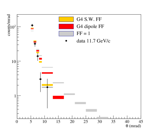
Figure 6: Comparison of the Monte Carlo simulation to the 11.7 GeV/c data-set. Data have been obtained by digitisation from the original paper[14].

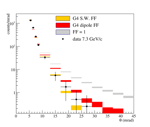
Figure 7: Comparison of the Monte Carlo simulation to the 7.3 GeV/c data-set. Data have been obtained by digitisation from the original paper[14].

VI-B Lead data with muons (Masek et al.)

The experiment[15] was performed in 1961 profiting of the Bevatron accelerator at the Lawrence radiation laboratory employing a muon beam with a median momentum of ($2.00~{}\pm~{}0.03$) GeV/c and a 3.5% spread. The total number of muons incident on the apparatus was $2.5\times 10^{7}$. The lead target had a thickness of 14.4 g/cm² corresponding to 1.268 cm (one half inch). Scattered particles were observed up to 12^∘ ($p_{T}~{}\simeq~{}400$ MeV/c). The muon beam is obtained from a $(3.5\pm 0.3)$ GeV/c pion beam with magnetic selection (see Fig. 3 of the original paper). 2 GeV/c muons are those decaying backward in the $\pi$ rest frame. This large difference in momentum allows a clean $\pi/\mu$ separation. The pion contamination on the target is estimated to be of about 3%. By using a 107 cm (42”) thick iron absorber downstream of the target and an upstream Cherenkov counter the effective pion contamination was reduced to $4.9\times 10^{-6}$. Emulsion detectors downstream of the target were also employed to control the pion contamination.

The incoming and outgoing muon directions were determined by using four identical counter hodoscopes made of scintillator bars at positions $A_{A}$, $A_{B}$, $A_{C}$ and $A_{D}$ (Fig. 3 of [15]). The acceptance of such an arrangement was between 2 and 14^∘. Each station was composed of 20 vertical scintillators each having dimensions (0.95, 2.54, 15.24) cm, the smallest dimension being the one in the horizontal plane. The downstream stations centers were shifted away from the beam direction by 26.2 cm. The distance along the beam between the stations was 2.794 m (AB) and 2.007 m (CD).

The beam spread in the horizontal and vertical directions was determined triggering with a small scintillator ($S$) located along the beam axis in between stations $A_{C}$ and $A_{D}$, rotating the $A_{A}$ and $A_{B}$ stations by 90^∘. The coincidence rate between strips in scintillators in $A_{A}$ and $A_{B}$ is shown in Fig. 6 of the original paper. This bidimensional rate map was used to generate the incoming direction of muons in the simulation accordingly. The vertical spread was generated assuming a gaussian distribution with a $\pm 0.6^{\circ}$ r.m.s. This is supported by the paper which states a spread of $\pm 0.8^{\circ}$ and $\pm 0.6^{\circ}$ in the horizontal and vertical views respectively. A gaussian fit of the $\theta_{x}$ distribution obtained from the information contained in the hit strip bidimensional distribution (Fig. 6 of [15]) and the detector geometry gives a spread of about 0.6^∘ not too far from the 0.8^∘ quoted in the paper.

We have reproduced with a simple simulation both the angular spread of the beam and the finite-solid angle effects introduced by the strip width. This was performed by binning the true positions according to the detector geometry described above. A simple linear trajectory has been assumed in between different scintillator stations.

The measured quantity is the angle $\Phi$ which is obtained considering the layout of hit strips in the scintillator counters which are only measuring the horizontal projection of the scattering angle (single-view readout). The distribution of $\Phi$ is shown in real data (bullets) and Monte Carlo (histograms) in Fig. 8. The meaning of the symbols is the same as in Figs. 6 and 7. The Monte Carlo normalisation corresponds to the same number of incoming muons as in the data (Tab. I). In this case both the point-like and the dipole form-factor simulations fail to describe the measurement while the modified simulation is capable of reproducing the experimental points at large scattering angles. The marked disagreement in the first bin is supposedly caused by the simplified simulation which might lack some of the geometrical details of the real apparatus.

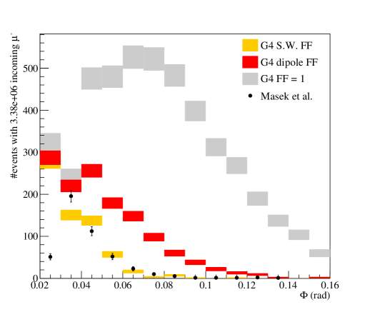
Figure 8: Comparison of the Monte Carlo simulation to the Masek et al. data-set.

VI-C Lead data with electrons (Frois et al.)

The experiment [11] was performed in 1977 at Saclay directing an electron beam with an energy of 502 MeV and a 20 $\mu$A current ($\sim 1.25\times 10^{14}~{}e$/s) on a water cooled $217\pm 2$ mg/cm² thick lead target. Thanks to the large event sample the data allowed a precision on the charge density at the lowest values of $r$ ever reached at those times or equivalently they allowed to determine the nuclear form factor at momentum transfers $q$ up to 3.5 fm^-1 (cross sections down to $10^{-10}$ mb/sr). The measured distribution of the momentum transfer $q$ spans over 12 decades (Fig. 9, bullets). The scattering angles were determined with an accuracy of 0.05^∘. The experimental points are compared in Fig. 9 with our simulation. In this case an event-by-event weighting was applied to the point-like distribution following the form-factor of Eq. 8 using the integral momentum transverse in the target as reweighing variable. This was dictated by the difficulty in adopting the single-scattering sampling approach within a reasonable amount of CPU time. It was verified anyway that the sampling approach correctly describes the experimental distribution up to $q\simeq$ 1 fm^-1. In the high-$q$ region the two approaches are expected to be very similar due to the prominence of single scatterings. The sharpness of the dips in the simulation is an artifact of the event-by-event instead of scattering-by-scattering form-factor reweighting.

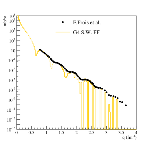
Figure 9: Comparison of the Monte Carlo simulation to Frois et al. data-set.

VII Large-angle muon scattering in the OPERA experiment

The large-angle scattering of muons from $\nu_{\mu}$ CC interactions represents a background for the $\tau\to\mu$ channel in the OPERA experiment at the CNGS neutrino beam. The kinematic selection described in the experiment proposal [16], [17] defines the signal region for the $\tau\to\mu$ search by requiring:

• $p_{T}^{\mu}>0.25$ GeV/c

• $\theta^{\mu}>20$ mrad

• $p_{\mu}>1$ and $p_{\mu}<15$ GeV/c

Furthermore the kink is asked to lie within the first two lead-emulsion layers downstream of the primary interaction vertex. One $\nu_{\tau}$ candidate in this decay channel was observed [18] with $p_{T}^{\mu}=(0.69\pm 0.05)$ GeV/c, $\theta^{\mu}=(245\pm 5)$ mrad and $p_{\mu}=(2.8\pm 0.2)$ GeV/c. In the experiment proposal [16, 17] some data-driven estimates of this process are reported. They are summarised in Fig. 10.

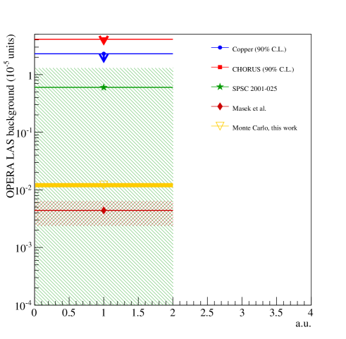
Figure 10: A compilation of experimental results on Large Angle muon Scattering. Bands represent $1\sigma$ confidence limits. The plot is discussed in the text.

The red arrow represents an upper limit from the non-observation of high-angle scattering in $1.5\times 10^{6}$ mm of muon tracks in the nuclear emulsions of the CHORUS experiment. This result was translated to 2 mm of Lead with the CNGS spectrum yielding [16] a 90% CL limit at $4.1\times 10^{-5}$. The blue line corresponds to the already described measurement on a Copper target (Sect. VI-A). A limit of $2.3\times 10^{-5}$ at 90% CL was obtained by extrapolating the observation to the case of scattering on Lead assuming a scaling going as $Z^{2}\rho/Ap^{2}$. The green hatched band was obtained from the observation of a single high-scattering event in the preliminary phase of a dedicated test-beam experiment [17] giving $0.6^{+0.7}_{-0.6}\times 10^{-5}$. In the proposal and later OPERA analyses the background has been finally assumed to be $1.0\times 10^{-5}/\nu_{\mu}^{CC}$ with a 50% relative error.

The contribution of LAS in this kinematic region was estimated using the simulation described in IV. A total number of about 1.1 billion incident $\mu^{-}$ have been generated with a flat momentum distribution between 1 and 15 GeV/c with orthogonal incidence on the lead-film double cell. The obtained distributions have then been reweighted in the incident muon momentum in order to reproduce the real spectrum of CNGS $\nu_{\mu}^{CC}$ events. The used reweighting function [19] (Fig. 11) reflects the expectation after applying the full selection chain used in the analysis [20].

It must be noted that in the real case of the OPERA experiment the momentum is determined with a certain resolution and that the selection cut $p_{T}>250$ MeV/c has to be taken on the reconstructed variable. The momentum resolution of muon tracks depends on whether the muon stops in the target or it exits from it. Furthermore if the track does not cross the spectrometer the only available determination comes from the analysis of multiple Coulomb scattering in the emulsion detectors. A very conservative estimate of the achievable resolution has been taken by considering a 15% Gaussian smearing in the $p^{-1}$ variable (See f.e. Fig. 91 of [16]).

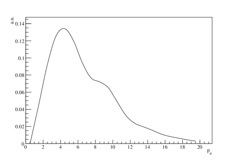
Figure 11: Spectrum of $\nu_{\mu}^{CC}$ CNGS events after selection used for reweighting the uniformly distributed momentum distribution used as an input to the simulation.

The scattering angle $\theta_{\mu}$ is defined as the difference in slope at the entrance and exit of the lead foil. We show in Fig. 12 the distributions of $\theta_{\mu}$ (top) and $p_{T}^{\mu}$ (bottom) before cuts (black), after the angular cut (red) and after the angular and $p_{T}$ cut (magenta). The numbers are break down as the cuts are applied in Tab. II.

	crossed cells	with $\theta>20$ mrad	and $p_{T}>0.25$ GeV/c
n.	2.22952 $\times 10^{9}$	1082520	115
weighted	3.05367 $\times 10^{9}$	365195	179.155
fraction	1	$2.4\times 10^{-4}/\nu_{\mu}^{CC}$	$(1.2\pm 0.1)\times 10^{-7}/\nu_{\mu}^{CC}$

TABLE II: Simulation results for the OPERA LAS background estimate including momentum reconstruction uncertainties.

The probability of having a LAS event in the signal region over two mm of Lead is then found to be: $f_{LAS}^{Pb}=(1.2\pm 0.1\rm{(stat.)})\times 10^{-7}/\nu_{\mu}^{CC}$ (yellow band in Fig. 10). The effect of momentum smearing convoluted with the observed distributions has a sensible effect since it increases the background due to migration of events in the high-$p_{T}$ region by bringing it from to $(6.8\pm 0.8)\times 10^{-8}/\nu_{\mu}^{CC}$ to $(1.2\pm 0.1)\times 10^{-7}/\nu_{\mu}^{CC}$.

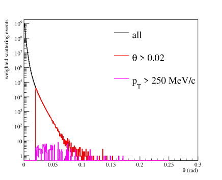
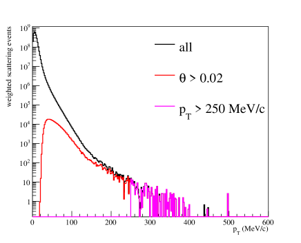
Figure 12: Distributions of $p_{T}^{\mu}$ (top) and $\theta_{\mu}$ (bottom) before cuts (black), after the angular cut (red) and after the angular and $p_{T}$ cuts (magenta).

A rough estimate of the OPERA LAS background can be also obtained by considering the data from Masek et al.[15] discussed in Sect. VI-B. In that case the muon momentum is 2 GeV/c which is included in the momentum range considered for the OPERA signal region ([1, 15] GeV/c). The thickness is 12.6 mm to be compared with the 2 mm of OPERA. The projected angle $\Phi$ is considered in that case. Muons with $p_{T}>250$ MeV/c will have approximately $\Phi>0.088$. On a sample of $2.5\times 10^{7}$ muons from the published binned distribution we can estimate the observation of (7 $\pm$ 3) events. Scaling linearly for the different thickness one can then estimate: $f_{LAS}^{Pb,Masek}\rm{(2~{}GeV/c)}=(0.44\pm 0.20)\times 10^{-7}/\nu_{\mu}^{CC}$ which lies even below the Monte Carlo result averaged in the [1, 15] GeV/c window (dark red band in Fig. 10).

VII-A Contribution of the scattering in other materials

The decay of the $\tau$ lepton is also considered when occurring in the emulsion films. For this reason we have also evaluated the LAS probability in these materials. Due to the high number of atomic components the implementation of Saxon-Woods nuclear form factors was not attempted in this case. For this reason we can take the results as an upper limit of the background. It must be also noted that for lighter nuclei the use of dipole form-factors, while remaining necessary, is less compelling than for the case of Lead. Each film is composed by a TAC (TriAcetylCellulose, C₂₈H₃₈O₁₉) 200 $\mu$m thick plastic base and by a pair of 50 $\mu$m thick emulsion layers on both sides of the base. The TAC has been modeled as a mixture of Carbon, Hydrogen and Oxygen in the proportion of 28:38:19. The detailed element budget for the emulsion layers [21] in terms of mass fraction is Ag 38.34%, Br 27.86%, C 13.00%, O 12.43%, N 4.81%, H 2.40%, I 0.81%, S 0.09%, Si 0.08%, Na 0.08%, K 0.05%, Sr 0.02%, Ba 0.01%. The results are: $f_{LAS}^{emul}<1.2\times 10^{-7}/\nu_{\mu}^{CC}$ and $f_{LAS}^{TAC}<0.7\times 10^{-7}/\nu_{\mu}^{CC}$.

VIII Muon photo-nuclear interactions in the OPERA experiment

For completeness we also try to estimate a possible contribution to the $\tau\to\mu$ background allowing for the possibility that it might arise from muon photo-nuclear interaction with an undetected hadronic remnant. At high enough muon energies ($E>10$ GeV), and at relatively high energy transfers e.g. when the energy lost by the muon, $\nu=E^{\prime}-E$, is more than a few % of its initial energy, the contribution from the inelastic interaction of muons with nuclei [23] starts to play a non negligible role.

The differential cross section $\sigma(E,\nu)$ (cm² g^-1 GeV^-1) can be factorised as $\sigma(E,\nu)=\Psi(\nu)\Phi(E,\nu)$ [24]. The first function, $\Psi$, reads:

$$\Psi(\nu)=\frac{\alpha}{\pi\nu}N_{A}\frac{A_{eff}}{A}\sigma_{\gamma N}$$ (9)

with $\sigma_{\gamma N}=(49.2+11.1\ln\nu+\frac{151.8}{\sqrt{\nu}})\times 10^{-30}$ cm² with $\nu$ in GeV [26]. The nuclear shadowing effect [25] is parametrised as $A_{eff}=0.22A+0.78A^{0.89}$ following [25] (0.65 for Lead). The adimensional function $\Phi$ depends on the fraction $v=E/\nu$ and $E$ as follows:

$$\begin{split}\Phi(E,\nu)=v-1+\left[1-v+\frac{v^{2}}{2}\left(1+\frac{2\mu^{2}}{\Lambda^{2}}\right)\right]\times\\ \ln\frac{\frac{E^{2}\left(1-v\right)}{\mu^{2}}\left(1+\frac{\mu^{2}v^{2}}{\Lambda^{2}\left(1-v\right)}\right)}{1+\frac{Ev}{\Lambda}\left(1+\frac{\Lambda}{2M}+\frac{Ev}{\Lambda}\right)}\end{split}$$ (10)

$M$ being the nucleon mass, $\mu$ the muon mass and $\Lambda^{2}=0.4$ GeV².

An energy-dependent scattering probability per incoming muon, $P_{\mu N}(E)$, is obtained after integration on $\nu$ and multiplication by $\rho t=1.135$ g cm^-2: $P_{\mu N}(E)=\rho t\int_{\nu_{min}}^{\nu_{max}}\Phi(E,\nu)d\nu$ with $\nu_{min}=0.2$ GeV and $\nu_{max}=E-M/2$ [28]. The result is shown by the black line curve in Fig. 13. In the same figure we show with the red line the cross section when one restricts to the phase space which is relevant for the OPERA background: the energy of the outgoing muon ($E^{\prime}=E-\nu$) should be $1<E^{\prime}<15$ GeV, the scattering angle ($\sin\theta=\frac{(E-E^{\prime})^{2}}{4(EE^{\prime}-\mu^{2})}$) should be $\theta>0.02$ rad and $E^{\prime}\sin\theta>0.25$ GeV. The result is then weighted with the probability density function of muons from $\nu_{\mu}^{CC}$ of CNGS muon neutrinos (Fig. 11 and dashed curve on Fig. 13) giving $f_{\mu N}=2.7\times 10^{-7}~{}{\rm{events}}/\nu_{\mu}^{CC}$ (also shown as a red dotted horizontal line in Fig. 13).

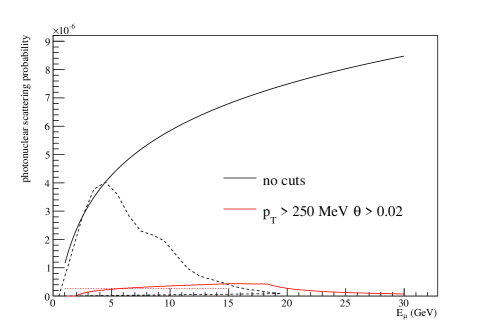
Figure 13: Photonuclear probability vs $E_{\mu}$.

It must be noted that this has to be considered as an upper limit to the real background level since a complete inefficiency in the detection of the hadronic system is assumed here for simplicity. Here we refrain from trying an estimate of the minimal hadronic activity which could be detected in the OPERA emulsion detectors since the contribution is already small enough for practical purposes.

IX Conclusions

The probability for the occurrence of large-angle scattering for multi-GeV muons in 1 mm thick lead targets has been addressed using a mixed-approach simulation program based on the GEANT4 libraries. A realistic parametrisation of the Lead nuclear density has been implemented (Saxon-Woods) and scattering off single protons has been considered. The developed algorithm has been validated by means of theoretical considerations and supported by experimental data from the literature. The simulation setup predicts a background for the OPERA $\nu_{\mu}\to\nu_{\tau}$ analysis in the $\tau\to\mu$ signal region of $f_{LAS}^{Pb}=(1.2\pm 0.1)\times 10^{-7}/\nu_{\mu}^{CC}$ which is well below the values which have been considered so far. Finally we also calculated, in the CNGS context, an upper limit on background contributions from the muon photo-nuclear process which might in principle also produce a large-angle muon scattering signature in the detector: $f_{\mu N}<2.7\times 10^{-7}~{}{\rm{events}}/\nu_{\mu}^{CC}$.

Appendix A Molière theory with nuclear effects (Meyer)

Given a target with thickness $t$, density $\rho$, atomic weight $A$, charge $Ze$ and an incoming particle of momentum $p$ with charge $ze$ we can define a “characteristic angle”, $\chi_{c}$, as

$$\chi_{c}=\frac{zZe^{2}}{p\beta c}\sqrt{\frac{4\pi N_{A}t\rho}{A}},$$ (11)

$N_{A}$ being Avogadro’s number. The “screening angle” ($\chi_{a}$) is defined from the De Broglie wave length of the incoming particle ($\lambda$) and the Thomas-Fermi radius of the atom ($a=0.53\times 10^{-10}~{}{\rm{m}}/Z^{1/3}$) as $\chi_{a}^{2}={\frac{\lambda}{2\pi a}}^{2}(1.13+3.76\alpha^{2})$ with $\alpha=\frac{2\pi zZe^{2}}{hv}$. Then the $B$ parameter of Eq. 3 is determined by the transcendental equation:

$$B=-\ln\left(\frac{\chi_{a}^{2}}{\chi_{c}^{2}}\frac{\hat{\gamma}^{2}}{\hat{e}B}\right)$$ (12)

where $\hat{e}$ and $\hat{\gamma}$ here are the Euler and Euler-Mascheroni numerical constants. The angle $\chi$ appearing in Eqns. 3 is $\chi=\frac{\theta}{\chi_{c}\sqrt{B}}$ . In the specific case of a 1mm thick Pb foil hit by a 10 GeV muon we find $\chi_{c}=0.24$ mrad, $\chi_{a}=1.61~{}\mu$rad and $B=14.7$. The coefficients $c_{i}$ for a nucleus with nuclear charge density $q(x)$ have the following expressions:

$$c_{0}=0.423+2\int_{0}^{\infty}(1-q(x))(1-e^{-x^{2}})x^{-3}dx$$ (13)

$$c_{1}=-1.423-2\int_{0}^{\infty}(1-q(x))e^{-x^{2}}x^{-1}dx$$ (14)

$$c_{2\nu}=\frac{2}{(\nu!)^{2}}\int_{0}^{\infty}q(x)x^{2\nu-3}e^{-x^{2}}dx$$ (15)

If a uniform charged sphere is assumed as in Eq. 4 and approximating the resulting form factor with a gaussian function $q=e^{-ax^{2}}$, the expression of the coefficients assumes this analytical form:

$$c_{0}=0.423-\left(1-\frac{1}{Z}\right)\left[\frac{a}{x_{n}^{2}}\ln\frac{a}{x_{n}^{2}}-\left(1+\frac{a}{x_{n}^{2}}\right)\ln\left(1+\frac{a}{x_{n}^{2}}\right)\right]$$ (16)

$$c_{1}=-1.423-\left(1-\frac{1}{Z}\right)\ln\left(1+\frac{a}{x_{n}^{2}}\right)$$ (17)

$$c_{2\nu}=\frac{(\nu-2)!}{(\nu!)^{2}}\left[\frac{1}{Z}+\left(1-\frac{1}{Z}\right)\left(1+\frac{a}{x_{n}^{2}}\right)^{1-\nu}\right]$$ (18)

References

- [1] S. Agostinelli et al., NIM A, vol. 506, no. 3, pp. 250-303, 2003.
- [2] J. Allison et al., IEEE Trans. Nucl. Sci., vol. 53, no. 1, pp. 270-278, 2006.
- [3] S. Goudsmit and J. L. Saudersons, Phys. Rev. 57 (1940) 24.
- [4] S. Goudsmit and J. L. Saudersons, Phys. Rev. 58 (1940) 36.
- [5] H. W. Lewis, Phys. Rev. 78 (1950) 526.
- [6] M. A. Meyer, Nucl. Phys. 28 (1961) 512-518.
- [7] G. Molière, Z. Naturforsh 3a, 1948, 78.
- [8] H. A. Bethe, Phys. Rev. 89 (1953), 1256.
- [9] G. Wentzel 1927 Z. Phys. 40 590
- [10] J. M. Fernandez-Varea, R. Mayol, J. Baro and F. Salvat, 1993 Nucl. Instr. Meth. B 73 447.
- [11] B. Frois et al., Phys. Rev. Lett. 38, 4, 152-155 (1977).
- [12] U. D. Jentschura, V. G. Serbo, Eur. Phys. J. C (2009) 64: 309-317
- [13] A.V. Butkevich et al. Nucl. Instrum. Meth. A 488 (2002) 282-294.
- [14] S. A. Akimenko et al., Nucl. Instr. Meth. A243 (1986) 518-522.
- [15] G. E. Masek et al., Phys. Rev. 122.937-948 (1961).
- [16] OPERA Coll., CERN-SPSC-2000-028, (1997).
- [17] OPERA Coll., CERN/SPSC 2001-025.
- [18] OPERA collaboration (N. Agafonova et al.), Phys. Rev. D89 (2014) 5, 051102.
- [19] A. Di Crescenzo, PhD thesis. Napoli Univ., April 2013. http://operaweb.lngs.infn.it/Opera/phpmyedit/theses-pub.php.
- [20] N. Agafonova et al, JHEP 1311 (2013) 036, Erratum-ibid. 1404 (2014) 014.
- [21] G. De Lellis, M. Komatsu, private communication.
- [22] L. Arrabito et al., 2007 JINST 2 P02001.
- [23] A.V. Butkevich et al., hep-ph/0109060.
- [24] V. V. Borog and A. A. Petrukhin, Proc. 14th Int. Conf. on Cosmic Rays, Munich,1975, vol.6, p.1949.
- [25] S. J. Brodsky, F. E. Close and J. F. Gunion, Phys. Rev. D6, 177 (1972).
- [26] D. O. Caldwell et al., Phys. Rev. Lett., 42, 553 (1979).
- [27] V. V. Borog, V. G. Kirillov-Ugryumov, A. A. Petrukhin, Sov. J. Nucl. Phys., 25, 1977, p.46.
-
[28]
http://geant4.cern.ch/G4UsersDocuments/UsersGuides/PhysicsReference
Manual/html/node49.html