Small-amplitude nonlinear modes under the combined effect of the parabolic potential, nonlocality and ${\cal PT}$ symmetry

Abstract

We consider nonlinear modes of the nonlinear Schrödinger equation with a nonlocal nonlinearity and an additional ${\cal PT}$-symmetric parabolic potential. We show that there exists a set of continuous families of nonlinear modes and study their linear stability in the limit of small nonlinearity. It is demonstrated that either ${\cal PT}$ symmetry or the nonlocality can be used to manage the stability of the small-amplitude nonlinear modes. The stability properties are also found to depend on the particular shape of the nonlocal kernel. Additional numerical simulations show that the stability results remain valid not only for the infinitesimally small nonlinear modes, but also for the modes of finite amplitude.

I Introduction

Nonlocal nonlinearities are known to be of relevance for numerous physical applications. In optical applications, nonlocal nonlinearity emerges in description of beam propagation in thermal media Litvak66 or in atomic vapors vapors . Nonlocal nonlinearities have been shown to support optical solitons Tur85 ; KrolBangSolitons ; XuKart05 ; Skupin06 and to alter their properties, such as, for instance, stability Tur85 , the collapse dynamics BangKrolCollapse , or the interactions between solitons DSNonlocal .

Nonlocality is also relevant in the theory of Bose-Einstein condensates (BECs) PS in view of the intrinsically nonlocal nature of the inter-atomic interactions Goral ; Sinha . Nonlocal nonlinearities are also inherent for plasma problems Litvak78 and for the theory on nematic crystals Assanto03 .

In many relevant situations, nonlocal nonlinearity is accompanied by a certain potential which models a confining trap for a BEC or a refractive index modulation in an optical waveguide. Presence of the external potential or nonlocality enriches the variety of possible nonlinear modes allowing to observe the so-called higher (alias multi-pole) nonlinear modes XuKart05 ; nonlin_homo apart from the best studied fundamental (alias ground state) nonlinear modes firstBEC ; KrolBangSolitons . Nonlocal nonlinearities have been considered in combination with the double-well Kevr2011 and the periodic potentials Kart_per ; Kart_per1 ; Cuevas . It looks however that a systematic study of nonlocal nonlinear modes in a parabolic potential has not been performed yet. In our present study, we make a step towards filling this gap and investigate nonlocal nonlinear modes in a complex parabolic ${\cal PT}$-symmetric potential of the form $V(x)=x^{2}-2i\alpha x$, where $\alpha$ is a real coefficient. For $\alpha=0$ the potential is reduced to the real parabolic potential whose modes are fairly well studied in the local case nonlin_homo ; AlZez , but have attracted much less attention in the nonlocal context.

For a nonzero $\alpha$, the potential $V(x)$ is complex and ${\cal PT}$ symmetric BendBoet , which is reflected by the fact that the real and imaginary parts of $V(x)$ are even and odd functions of $x$, respectively. ${\cal PT}$ symmetry can be implemented in diverse physical setting, including optics Ruter , atomic gases HHK , and BECs KGM08 .

Nonlinear modes and solitons have been studied in various ${\cal PT}$-symmetric potentials with local Musslimani_1 ; PTfamiliesLocal ; ZezKon12 and nonlocal PTNonlocal nonlinearities, but the present work has a slightly peculiar focus. We are particularly interested in the examining the combined effect of the parabolic trapping, nonlocality and ${\cal PT}$ symmetry on the excited (higher-order) nonlinear modes. The focus of our study is additionally shifted towards the existence and stability of small-amplitude nonlinear modes, whose properties can be studied by means of asymptotic expansions describing bifurcations of nonlinear modes from the eigenstates of the underlying linear model. The linear spectrum of the ${\cal PT}$-symmetric parabolic potential is available in the analytical, which makes it possible to reduce the stability problem to computing the real zeros of certain analytical expressions. Our analysis shows that either the degree of the nonlocality or the strength of the ${\cal PT}$ symmetry can be used to manage the stability of the excited modes. On the other hand, we reveal a dependence of the stability properties on the particular shape of the nonlocal kernel. We also touch upon the properties of nonlinear modes of finite amplitude and illustrate numerically that the stability results hold not only for the infinitesimally small nonlinear modes but also remain valid in a finite range of the amplitudes of nonlinear modes.

The paper is organized as follows. In the next section, we present a model to be considered throughout the paper. In Sec. III we describe the linear properties of the model and introduce the families of small-amplitude nonlinear modes. In Sec. IV we describe the methodology of the linear stability analysis. The main results of stability analysis are presented in Sec. V and Sec. VI for the conservative and ${\cal PT}$-symmetric cases, respectively. In Sec. VII we demonstrate numerically that the presented asymptotical stability results persist in a finite range of the amplitude of the modes. Concluding Sec. VIII outlines the main results of the work.

II The models

We use the dimensionless nonlocal nonlinear Schrödinger equation with an additional parabolic potential and nonlocal nonlinearity:

$$i\frac{\partial q(x,z)}{\partial z}=-\frac{\partial^{2}q(x,z)}{\partial x^{2}}+(x^{2}-2i\alpha x)q(x,z)$$

$$-\sigma q(x,z)\int_{-\infty}^{\infty}K(x-x^{\prime})|q(x^{\prime},z)|^{2}dx^{\prime}.$$ (1)

The case $\alpha=0$ corresponds to the real parabolic potential, while nonzero $\alpha$ governs the strength of the ${\cal PT}$ symmetry. The system is subject to gain in the domain $x<0$ and is subject to losses for $x>0$. In the optical context, equation (II) models beam guidance in a medium whose refractive index $n(x)=n_{r}(x)+in_{i}(x)$ has parabolic modulation of the real part $n_{r}(x)=x^{2}$, and linear modulation of the imaginary part $n_{i}=2\alpha x$. Equation (II) with $\alpha=0$ also arises as a Gross-Pitaevskii equation PS in the mean-field theory the harmonically trapped a quasi-one-dimensional BEC Goral ; quasi-collapse ; Cuevas . In this case, $q(x,z)$ is a quasi-one-dimensional wavefunction Sinha , and $z$ plays a role of time. Sign $\sigma=\pm 1$ corresponds to attractive (focusing) and repulsive (defocusing) nonlinearities, respectively. Nonlocal properties of the model are described by the kernel $K(x)$ which is a positive function with normalization $\int K(x)dx=1$ (hereafter all the integrals are taken over the whole real axis). Following to the previous studies on the subject XuKart05 ; Skupin06 ; Kart_per1 ; Kevr2011 , we pay the primary attention to the following two kernels:

(i) The smooth Gaussian kernel

$$K(x)=\frac{1}{\sqrt{\pi}\lambda}e^{-x^{2}/\lambda^{2}}$$ (2)

where $\lambda>0$ governs strength of nonlocality.

(ii) Exponential kernel with the singularity at $x=0$:

$$K(x)=\frac{1}{2\lambda}e^{-|x|/\lambda}.$$ (3)

(iii) It will be also interesting to compare the obtained results with a slowly (algebraically) decaying kernel. While some studies (for example, Kevr2011 ; Cuevas ) deal with the so-called cut-off (CO) kernel which decays as $|x|^{-3}$ as $x\to\pm\infty$, in our study we choose the algebraically decaying Lorentzian kernel (the Lorentzian)

$$K(x)=\left\{\begin{array}[]{c}\frac{\lambda}{\pi(\lambda^{2}+x^{2})}\mbox{\quad if }\lambda>0,\\[5.69054pt] \delta(x)\mbox{\quad\quad if }\lambda=0.\end{array}\right.$$ (6)

This choice is motivated by the fact that the Lorentzian kernel (6) allows for the relatively simple analytical evaluation of the convolution integrals that arise in what follows.

III Bifurcations of nonlinear modes

The stationary nonlinear modes for Eq. (II) admit the representation $q(x,z)=e^{i\beta z}w(x)$, where $\beta$ is a real parameter. It is convenient to introduce the shifted parameter $b$ defined through the relation $\beta=b-\alpha^{2}$, which allows to rewrite the equation for the nonlinear modes in the following form:

$$w_{xx}-bw-(x-i\alpha)^{2}w\hskip 85.35826pt$$

$$+\sigma w(x)\int_{-\infty}^{\infty}K(x-x^{\prime})|w(x^{\prime})|^{2}dx^{\prime}=0,$$ (7)

subject to the zero boundary conditions at the infinity: $\lim_{x\to\pm\infty}w(x)=0$.

Let us first recall the properties of the underlying linear problem which formally corresponds to $\sigma=0$ in Eq. (III). The resulting equation which is considered as a linear eigenvalue problem for $b$ and $w(x)$, has a purely real and discrete spectrum Kato ; Znoj1 ; ZezKon12 . The eigenvalues $\tilde{b}_{n}$ can be listed as $\tilde{b}_{n}=-(2n+1)$, $n=0,1,\ldots$. The corresponding eigenfunctions $\tilde{w}_{n}(x)$ read

$$\tilde{w}_{n}(x)=c_{n}H_{n}(x-i\alpha)e^{-(x-i\alpha)^{2}/2},$$ (8)

$$c_{n}=\frac{e^{-\alpha^{2}/2}}{\sqrt{\sqrt{\pi}2^{n}n!G_{n}(-2\alpha^{2})}}$$ (9)

where $H_{n}(x)$ and $G_{n}(x)$ are Hermite and Laguerre polynomials AS , respectively. The choice of the coefficients $c_{n}$ implies normalization $\int|\tilde{w}_{n}|^{2}dx=1$. Each Hermite polynomial $H_{n}(x)$ contains only powers of $x$ of the same parity as the number $n$. This implies that in the conservative limit ($\alpha=0$) the eigenfunctions are real-valued functions which have exactly $n$ zeros and have the same parity as the number $n$. For $\alpha\neq 0$, each eigenfunction $\tilde{w}_{n}(x)$ possesses real even part and odd imaginary part for even $n$ and odd real part and even imaginary part for odd $n$.

Returning now to the nonlinear problem, we look for bifurcations of small-amplitude nonlinear modes from the linear eigenstates. To this end, we introduce the formal asymptotic expansions which describe nonlinear modes $w_{n}(x)$ branching off from the zero solution $w(x)\equiv 0$ at the eigenvalues $\tilde{b}_{n}$ ZezKon12 :

$$w_{n}(x)=\varepsilon\tilde{w}_{n}+\varepsilon^{3}w_{n}^{(3)}+\mathcal{O}(\varepsilon^{5}),\quad b_{n}=\tilde{b}_{n}+\sigma\varepsilon^{2}b_{n}^{(2)}+o(\varepsilon^{2}),$$ (10)

where $\varepsilon\ll 1$ is a formal small real parameter (for the rigorous analysis of the bifurcations of small-amplitude modes see DS15 ).

Since $\tilde{w}_{n}(x)$ are normalized, the squared $L^{2}$-norm of the nonlinear modes $U=\int|w_{n}(x)|^{2}dx$ (which is also associated with the total energy flow in the optical applications of the model) is approximately equal to $\varepsilon^{2}$: $U\approx\varepsilon^{2}$ for $\varepsilon\ll 1$. Substituting expansions (10) into Eq. (III) and collecting the terms of the $\varepsilon^{3}$-order, one arrives at an inhomogeneous linear differential equation with respect to the function $w_{n}^{(3)}$. The solvability condition for the latter equation yields the expression for the coefficient $b_{n}^{(2)}$:

$$b_{n}^{(2)}=\frac{\int\tilde{w}_{n}^{2}(x)\left(\int K(x-x^{\prime})|\tilde{w}_{n}(x^{\prime})|^{2}dx^{\prime}\right)dx}{\int\tilde{w}_{n}^{2}(x)dx}.$$ (11)

For the conservative case ($\alpha=0$) the eigenfunctions $\tilde{w}_{n}(x)$ are real, and hence the coefficients $b_{n}^{(2)}$ are obviously real too for any $n$. For $\alpha\neq 0$, the eigenfunctions $\tilde{w}_{n}(x)$ possess nontrivial real and imaginary parts as described above. However, parities of real and imaginary parts of $\tilde{w}_{n}(x)$ imply that for a real and even kernel function $K(x)=K(-x)=K^{*}(x)$ the coefficients $b_{n}^{(2)}$ are also real, which shows that continuous families of nonlinear modes can exist in the ${\cal PT}$-symmetric model with $\alpha>0$. The family with $n=0$ represents the fundamental nonlinear modes, and the families $n=1,2,\ldots$ contain the higher-order modes.

IV Linear stability of nonlinear modes

IV.1 Statement of the problem

Following to the the standard procedure of the linear stability analysis, we consider a perturbed nonlinear mode $w_{n}(x)$ in the form $q(x,z)=e^{i\beta z}[w_{n}(x)+u(x)e^{i\omega z}+v^{*}(x)e^{-i\omega^{*}z}]$ which after linearization with respect to small functions $u(x)$ and $v(x)$ gives the linear stability eigenvalue problem

$${L}\,{\bf p}=\omega\,{\bf p},\quad{\bf p}=\left(\!\begin{array}[]{c}u\\ v\end{array}\!\right),$$ (12)

with the linear operator $L$ given as

$${L}=\left(\!\!\begin{array}[]{cc}A&\sigma w_{n}{\cal K}_{w_{n}}\\[5.69054pt] -\sigma w_{n}^{*}{\cal K}_{w_{n}^{*}}&-A^{\dagger}\end{array}\!\!\right),$$

where

$$A = {\cal L}+\sigma({\cal K}|w_{n}|^{2})+\sigma w_{n}{\cal K}_{w^{*}_{n}},$$ (14)

$$A^{\dagger} = {\cal L}^{\dagger}+\sigma({\cal K}|w_{n}|^{2})+\sigma w_{n}^{*}{\cal K}_{w_{n}},$$ (15)

$${\cal L} = d^{2}/dx^{2}-b-(x-i\alpha)^{2},$$ (16)

$${\cal L}^{\dagger} = d^{2}/dx^{2}-b-(x+i\alpha)^{2},$$ (17)

${\cal K}$ is the convolution operator, i.e., ${\cal K}p=\int K(x-x^{\prime})p(x^{\prime})dx^{\prime}$, and ${\cal K}_{p}$ is the operator of “weighted” convolution, i.e., ${\cal K}_{p}\,q={\cal K}(p\,q)=\int K(x-x^{\prime})p(x^{\prime})q(x^{\prime})dx^{\prime}$.

The nonlinear mode $w_{n}(x)$ is said to be linearly unstable if operator $L$ has at least one eigenvalue $\omega$ such that $\textrm{Im\ }\omega<0$. Otherwise, $w_{n}(x)$ is linearly stable.

IV.2 Linear stability of small-amplitude modes

Let us now analyze the spectrum of the operator ${L}$ for small-amplitude nonlinear modes belonging to the $n$th family and situated in the vicinity of the bifurcation from the linear limit. For nonlinear modes of zero amplitude (i.e., for $\varepsilon=0$) the operator ${L}$ acquires the diagonal form

$${L}=\tilde{{L}}_{n}=\left(\begin{array}[]{cc}{\cal L}_{n}&0\\ 0&-{\cal L}_{n}^{\dagger}\end{array}\right),$$ (18)

where

$${\cal L}_{n}=\frac{d^{2}\ }{dx^{2}}-\tilde{b}_{n}-(x-i\alpha)^{2},$$ (19)

$${\cal L}_{n}^{\dagger}=\frac{d^{2}\ }{dx^{2}}-\tilde{b}_{n}-(x+i\alpha)^{2}.$$ (20)

Since the spectrum of the operator ${\cal L}_{n}+\tilde{b}_{n}$ is known from the discussion in Sec. III, it is easy to deduce that the spectrum of the operator $\tilde{{L}}_{n}$ consists of two subsets. Eigenvalues and eigenvectors of the first subset read $\omega^{(I)}_{n,k}=2(n-k)$, ${\bf p}^{(I)}_{n,k}=(\tilde{w}_{k}(x),0)^{T}$, $k=0,1,\ldots$. The second sequence reads $\omega^{(II)}_{n,k}=-2(n-k)$, ${\bf p}^{(II)}_{n,k}=(0,\tilde{w}_{k}^{*}(x))^{T}$, $k=0,1,\ldots$.

Thus, operator $\tilde{{L}}_{n}$ has a double zero eigenvalue $\omega^{(I)}_{n,n}=\omega^{(II)}_{n,n}=0$ which remains zero and double when passing from the linear limit $\varepsilon=0$ to $\varepsilon>0$ ZezKon12 . The operator $\tilde{{L}}_{n}$ also has $2n$ double nonzero eigenvalues: $\Omega_{n,k}=\omega^{(I)}_{n,k}=\omega^{(II)}_{n,2n-k}$, where $k$ runs from 0 to $2n$ except for $k=n$. Each double eigenvalue $\Omega_{n,k}$ is semi-simple; the two corresponding linearly independent eigenvectors are given as

$${\bf p}^{(I)}_{n,k}=\left(\begin{array}[]{c}\tilde{w}_{k}\\ 0\end{array}\right)\mbox{\quad and\quad}{\bf p}^{(II)}_{n,2n-k}=\left(\begin{array}[]{c}0\\ \tilde{w}_{2n-k}^{*}\end{array}\right).$$ (21)

Passing from the linear limit $\varepsilon=0$ to small nonzero $\varepsilon$, each double eigenvalue $\Omega_{n,k}$ generically splits into two simple eigenvalues which will be either both real or complex conjugated. If each double eigenvalue splits into two real ones, then the small-amplitude modes belonging to the $n$th family are stable for both attractive and repulsive nonlinearities. Vice versa, if at least one double eigenvalue gives birth to a pair of two complex-conjugated simple eigenvalues, then the small-amplitude nonlinear modes of the $n$th family are unstable. Notice also that for $n=0$ no double eigenvalues $\Omega_{n,k}$ exists. Therefore the fundamental solutions from family $n=0$ are always stable in the small-amplitude limit.

It is easy to check that the eigenvalue $\Omega_{n,k}$ splits in exactly the same way as the opposite double eigenvalue $\Omega_{n,2n-k}=-\Omega_{n,k}$, i.e., if $\Omega_{n,k}$ splits into two real eigenvalues then $\Omega_{n,2n-k}$ also splits into two real eigenvalues and vice versa. Therefore, in order to examine stability of small-amplitude nonlinear modes that belong to the $n$th family, it is sufficient to analyze only $n$ positive double eigenvalues $\Omega_{n,k}$ with $k=0,\ldots,n-1$.

In order to examine splitting of the double eigenvalues $\Omega_{n,k}$, we employ Eqs. (10) which yield the following asymptotic expansion for the linear stability operator: ${L}=\tilde{{L}}_{n}+\sigma\varepsilon^{2}{L}_{n}^{(2)}+o(\varepsilon^{2})$, where the correction ${L}_{n}^{(2)}$ is given as

$$\left(\!\!\begin{array}[]{cc}-b_{n}^{(2)}+({\cal K}|\tilde{w}_{n}|^{2})+\tilde{w}_{n}{\cal K}_{\tilde{w}^{*}_{n}}&\tilde{w}_{n}{\cal K}_{\tilde{w}_{n}}\\ -\tilde{w}_{n}^{*}{\cal K}_{\tilde{w}_{n}^{*}}&b_{n}^{(2)}-({\cal K}|\tilde{w}_{n}|^{2})-\tilde{w}_{n}^{*}{\cal K}_{\tilde{w}_{n}}\end{array}\!\!\right).$$

Following the standard arguments of the perturbation theory for linear operators Kato , in order to address the splitting of the double eigenvalue $\Omega_{n,k}$ we consider a $2\times 2$ matrix defined as

$${M}_{n,k}=\left(\!\!\begin{array}[]{cc}\displaystyle\frac{\langle{L}_{n}^{(2)}{\bf p}^{(I)}_{n,k},{{\bf p}^{(I)*}_{n,k}}\rangle}{\langle{\bf p}^{(I)}_{n,k},{{\bf p}^{(I)*}_{n,k}}\rangle}&\displaystyle\frac{\langle{L}_{n}^{(2)}{\bf p}^{(II)}_{n,2n-k},{{\bf p}^{(I)*}_{n,k}}\rangle}{\langle{\bf p}^{(I)}_{n,k},{{\bf p}^{(I)*}_{n,k}}\rangle}\\[17.07164pt] \displaystyle\frac{\langle{L}_{n}^{(2)}{\bf p}^{(I)}_{n,k},{{\bf p}^{(II)*}_{n,2n-k}}\rangle}{\langle{\bf p}^{(II)}_{n,2n-k},{{\bf p}^{(II)*}_{n,2n-k}}\rangle}&\displaystyle\frac{\langle{L}_{n}^{(2)}{\bf p}^{(II)}_{n,2n-k},{{\bf p}^{(II)*}_{n,2n-k}}\rangle}{\langle{\bf p}^{(II)}_{n,2n-k},{{\bf p}^{(II)*}_{n,2n-k}}\rangle}\end{array}\!\!\right),$$

where $\langle{\bf a},{\bf b}\rangle=\int{\bf b}^{\dagger}(x){\bf a}(x)dx$ for any two column vectors ${\bf a}$ and ${\bf b}$ (here ^† means the transposition and complex conjugation). If both the eigenvalues of matrix ${M}_{n,k}$ are real, then the double eigenvalue $\Omega_{n,k}$ splits into two real and simple eigenvalues. If such a situation takes place for all $k=0,1,\ldots,n-1$, then the small-amplitude nonlinear modes $w_{n}(x)$ from the $n$th family are stable. On the other hand, if for some $k$ the matrix ${M}_{n,k}$ has a complex eigenvalue, then the double eigenvalue $\Omega_{n,k}$ splits into a pair of complex-conjugated eigenvalues. This is sufficient to conclude that the small-amplitude nonlinear modes from the $n$th family are unstable.

Recall that real and imaginary parts of $\tilde{w}_{n}(x)$ have opposite parities. Using this fact, one can establish that all the entries of the matrices ${M}_{n,k}$ are real numbers which read

$$\left({M}_{n,k}\right)_{1,1}=-b_{n}^{(2)}+\hskip 113.81102pt$$

$$\frac{\int\tilde{w}_{k}\{\tilde{w}_{k}{\cal K}_{\tilde{w}_{n}^{*}}\tilde{w}_{n}+\tilde{w}_{n}{\cal K}_{\tilde{w}_{n}^{*}}\tilde{w}_{k}\}\ dx}{\int\tilde{w}_{k}^{2}dx},$$ (23)

$$\left({M}_{n,k}\right)_{2,2}=b_{n}^{(2)}-\hskip 122.34692pt$$

$$\frac{\int\tilde{w}_{2n-k}\{\tilde{w}_{2n-k}{\cal K}_{\tilde{w}_{n}^{*}}\tilde{w}_{n}+\tilde{w}_{n}{\cal K}_{\tilde{w}_{n}^{*}}\tilde{w}_{2n-k}\}\ dx}{\int\tilde{w}_{2n-k}^{2}dx},$$ (24)

$$\left({M}_{n,k}\right)_{2,1}=-\frac{\int\tilde{w}_{n}\tilde{w}_{2n-k}{\cal K}_{\tilde{w}_{n}}\tilde{w}_{k}^{*}\ dx}{\int\tilde{w}_{2n-k}^{2}dx},$$ (25)

$$\left({M}_{n,k}\right)_{1,2}=\frac{\int\tilde{w}_{n}\tilde{w}_{k}{\cal K}_{\tilde{w}_{n}}\tilde{w}_{2n-k}^{*}\ dx}{\int\tilde{w}_{k}^{2}dx}.$$ (26)

Thus in order to check reality of the eigenvalues of the matrix ${M}_{n,k}$, it is sufficient to consider the discriminant of its quadratic characteristic equation, i.e., the quantity $D_{n,k}=\left[({M}_{n,k}\right)_{1,1}+\left({M}_{n,k}\right)_{2,2}]^{2}-4\det{M}_{n,k}$. For $D_{n,k}>0$ the eigenvalues of ${M}_{n,k}$ are real while a situation with $D_{n,k}<0$ corresponds to a pair of complex conjugated eigenvalues. The situation $D_{n,k}=0$ requires a more delicate analysis as in this case behavior of the double eigenvalue $\Omega_{n,k}$ is determined by the next terms of the asymptotic expansions.

Using analytical expressions for the eigenfuctions $\tilde{w}_{n}(x)$, the entries of matrices ${M}_{n,k}$ and hence the determinant $D_{n,k}$ can be computed analytically with a computer algebra program (at least, for several relevant shapes of the kernel function $K(x)$). The resulting analytical expressions are too bulky to be presented in the paper. However, for an interested reader to have an idea of how the expressions for the determinants $D_{n,k}$ read, in Appendix A we provide two expressions for $D_{1,0}$ and $D_{2,0}$ obtained for the Gaussian kernel and $\alpha=0$. Complexity of the expressions for $D_{n,k}$ increases drastically if larger numbers $n$ or nonzero values of $\alpha$ are involved. Nevertheless, these expressions are available analytically and can be used for finding the domains of positivity and negativity of the determinants $D_{n,k}$ which are considered as functions of $\lambda$ and $\alpha$.

V Results for the real parabolic potential

Let us start presentation of our results with an important particular case $\alpha=0$, when ${\cal PT}$-symmetric contribution is absent, and the model is conservative. First, it is relevant to notice that for $\alpha=0$ the eigenvalue problem (12) admits an exact solution with eigenvalue $\omega=2$ and the respective eigenvector given as

$${\bf p}=\left(\begin{array}[]{c}\phantom{+}xw_{n}+w_{n}^{\prime}\\ -xw_{n}+w_{n}^{\prime}\end{array}\right).$$ (27)

Notice however that this exact solution does not hold for nonzero $\alpha$.

Results of linear stability analysis of small-amplitude nonlinear modes from several first families for the Gaussian kernel (2) are summarized in Table 1. For $n=1,2,\ldots 6$ and for $k=0,1,\ldots,n-1$, Table 1 reports sign of the determinant $D_{n,k}$ in the local limit $\lambda=0$ and the approximated values of positive zeros of determinants $D_{n,k}$ being considered as functions of $\lambda$ [at the same time, those are the values of $\lambda$ at which functions $D_{n,k}=D_{n,k}(\lambda)$ change their signs]. From Table 1 one can recover information on stability or instability of the small-amplitude nonlinear modes bifurcating from the $n$th linear eigenstate for the given value of the nonlocality parameter $\lambda$: the stability takes place if $D_{n,k}(\lambda)>0$ for each $k=0,1,\ldots,n-1$.

It follows from Table 1 that for $n=1$ and $k=0$ the respective determinant $D_{1,0}(\lambda)$ is positive for any $\lambda\geq 0$ (see also the explicit expression (33) for $D_{1,0}$ in Appendix A). Therefore, the small-amplitude nonlinear modes bifurcating from the linear eigenstate $n=1$ are stable for any $\lambda\geq 0$. The small-amplitude modes with $n=2$ are unstable for $0\leq\lambda\lesssim 1.82$ but become stable for $\lambda\gtrsim 1.82$. For $n>2$ the stability situation might be more complex with the half-axis $\lambda\geq 0$ divided into several alternating intervals of stability and instability. In the local case ($\lambda=0$) all the higher-order small-amplitude mode are unstable for $n\geq 2$ AlZez . However, from Table 1 one observes that for each $n$ there exists a threshold value $\Lambda_{n}$ such that the small-amplitude modes become stable for the sufficiently strong nonlocality $\lambda>\Lambda_{n}$. The specific values of $\Lambda_{n}$ can be recovered from Table 1: $\Lambda_{1}=0$, $\Lambda_{2}\approx 1.82$, $\Lambda_{3}\approx 2.36$, etc. Thus the sufficiently strong nonlocality essentially alters (enhances) stability of the excited modes.

We additionally mention that for each $n$ one has $D_{n,n-1}(\lambda)>0$ for all $\lambda$. This is a consequence of the exact solution (27) which implies that the spectrum of operator $L$ always contains an eigenvalue equal to $2$. Therefore, the double eigenvalue $\Omega_{n,n-1}=2$ always splits in the pair of real eigenvalues (one of which is equal to $2$). As a result, the eigenvalue $\Omega_{n,n-1}$ can not cause instability of small-amplitude nonlinear modes.

Table 1: Results of linear stability analysis for $\alpha=0$ and the Gaussian kernel.

n	k	$\textrm{sign}\left.D_{n,k}(\lambda)\right|_{\lambda=0}$	zeros of $D_{n,k}(\lambda)$ (if any)
1	0	$+$	no zeros
2	0	$-$	1.82
	1	$+$	no zeros
3	0	$-$	2.36
	1	$-$	2.04
	2	$+$	no zeros
4	0	$+$	2.61  2.85
	1	$-$	2.64
	2	$-$	2.26
	3	$+$	no zeros
5	0	$+$	3.23  3.25
	1	$-$	3.12
	2	$-$	2.90
	3	$-$	2.45
	4	$+$	no zeros
6	0	$+$	3.566  3.568
	1	$+$	3.45  3.51
	2	$-$	3.37
	3	$-$	3.13
	4	$-$	2.64
	5	$+$	no zeros

Let us now turn to examination of other kernel functions $K(x)$. The results of linear stability analysis for the exponential kernel (3) are reported in Table 2 which features an essentially different stability picture comparing to that for the Gaussian kernel. Specifically, we observe that for the exponential kernel in the limit of strong nonlocality $\lambda\to\infty$, only the small-amplitude modes with $n=0,1,2$ are stable, whereas the modes with $n\geq 3$ are unstable both in the local limit $\lambda=0$ and for all positive $\lambda$.

To summarize the intermediate results obtained so far, we have encountered different stability situations for two different shapes of the kernel $K(x)$. In the case of the smooth Gaussian kernel, small-amplitude nonlinear modes bifurcating from the $n$th linear state become stable in the limit of high nonlocality for any $n$. On contrary, for the exponential kernel the small-amplitude modes are stable in the strongly nonlocal limit only for $n\leq 2$ and unstable for $n\geq 3$. The found difference in stability situation of strongly nonlocal modes reveals certain correspondence to the previous results on the stability of the high-order nonlocal nonlinear states, such as multipole-mode 1D solitons XuKart05 and 2D spatial solitons Skupin06 . Both XuKart05 and Skupin06 report that stable higher-order states can be found in the case of the Gaussian kernel, while the exponential kernel results in instability of all high order solitons, starting from some threshold order. It has been also suggested in Skupin06 that the mentioned difference between Gaussian and exponential kernels is related to the singularity which the exponential kernel has at the origin $x=0$. Our approach allows to substantiate the above suggestion. Indeed, for the Gaussian kernel one can establish asymptotic behavior of entries of the matrix $M_{n,k}$ in the limit $\lambda\to\infty$. Specifically, for $\lambda\to\infty$ one has

$$(M_{n,k})_{1,1},(M_{n,k})_{2,2}, \propto \lambda^{-3},$$ (28)

$$(M_{n,k})_{2,1},(M_{n,k})_{1,2} \propto \lambda^{-(2n-2k+1)}.$$ (29)

Technical details on computing the asymptotics (28)–(29) are presented in Appendix D. Additionally, in Appendices B and C we provide auxiliary relations necessary for the derivation of (28)–(29).

Relations (28)–(29) immediately imply that in the limit of large $\lambda$ for $k=0,1,\ldots,n-2$ the diagonal elements of the matrix $M_{n,k}$ dominate the off-diagonal elements, which guarantees reality of the eigenvalues of $M_{n,k}$. Since the instability never occurs for $k=n-1$ [due to the presence of the exact solution (27), as discussed above], we confirm that for the Gaussian kernel (or, more generally, for an infinitely differentiable kernel) the small-amplitude modes of arbitrarily high order $n$ are stable in the limit of the strong nonlocality.

At the same time, asymptotic results (28)–(29), generically speaking, do not hold for a non-differentiable kernel. For example, for the exponential kernel we have computed that for $n=3$ and $k=0$ all the entries of the matrix $M_{n,k}$ behave as $\propto\lambda^{-2}$ for $\lambda\to\infty$, i.e., the diagonal domination in the strongly nonlocal limit is not guaranteed.

Table 2: Results of linear stability analysis for $\alpha=0$ and the exponential kernel.

n	k	$\textrm{sign}\left.D_{n,k}(\lambda)\right|_{\lambda=0}$	zeros of $D_{n,k}(\lambda)$
1	0	$+$	no zeros
2	0	$-$	1.31
	1	$+$	no zeros
3	0	$-$	no zeros
	1	$-$	1.54
	2	$+$	no zeros
4	0	$+$	7.25
	1	$-$	no zeros
	2	$-$	1.70
	3	$+$	no zeros
5	0	$+$	no zeros
	1	$-$	no zeros
	2	$-$	no zeros
	3	$-$	1.84
	4	$+$	no zeros
6	0	$+$	no zeros
	1	$+$	no zeros
	2	$-$	no zeros
	3	$-$	no zeros
	4	$-$	1.97
	5	$+$	no zeros

Table 3: Results of linear stability analysis for $\alpha=0$ and the Lorentzian kernel.

n	k	$\textrm{sign}\left.D_{n,k}(\lambda)\right|_{\lambda=0}$	zeros of $D_{n,k}(\lambda)$
1	0	$+$	no zeros
2	0	$-$	1.52
	1	$+$	no zeros
3	0	$-$	2.70
	1	$-$	1.66
	2	$+$	no zeros
4	0	$+$	2.77  3.446
	1	$-$	2.96
	2	$-$	1.77
	3	$+$	no zeros
5	0	$+$	3.88  3.991
	1	$-$	3.74
	2	$-$	3.21
	3	$-$	1.87
	4	$+$	no zeros
6	0	$+$	4.39  4.42
	1	$+$	3.98  4.28
	2	$-$	4.00
	3	$-$	3.44
	4	$-$	1.97
	5	$+$	no zeros

Table 3 which reports the stability analysis for the algebraically depending kernel (6) further confirms the stability of strongly nonlocal high-order small-amplitude modes for an infinitely differentiable kernel. Besides of this, we have also performed the same linear stability analysis for several nonphysical but still illustrative nonlocal kernels such as a rectangular kernel with finite support

$$K(x)=\left\{\begin{array}[]{cc}\frac{1}{2\lambda}&\mbox{for }x\in(-\lambda,\lambda)\\ 0&\mbox{otherwise,}\end{array}\right.$$ (30)

a triangular shaped kernel with finite support

$$K(x)=\left\{\begin{array}[]{cc}\frac{x}{\lambda^{2}}+\frac{1}{\lambda}&\mbox{for }x\in(-\lambda,0)\\ \frac{-x}{\lambda^{2}}+\frac{1}{\lambda}&\mbox{for }x\in(0,\lambda)\\ 0&\mbox{otherwise,}\end{array}\right.$$ (31)

and a smooth exponentially decaying kernel

$$K(x)=\frac{e^{-1/4}}{4\lambda}\left(\textrm{erfc}\left(\frac{-x}{\lambda}\right)e^{-x/\lambda}+\textrm{erfc}\left(\frac{x}{\lambda}\right)e^{x/\lambda}\right)$$ (32)

[the particular choice of the kernels (30)–(32) is motivated by convenience of analytical evaluation of the respective convolution integrals]. Kernels (30) and (32) also feature stabilization of all higher-order strongly nonlocal modes, whereas for the triangular kernel (31) the higher-order strongly nonlocal modes are unstable. This allows to conclude that the main feature responsible for the stability is not the very presence of the singularity of the kernel, but the location of the singularity: the rectangular kernel (30) features two discontinuities at $x=\pm\lambda$ but its behavior is nevertheless similar to that of the Gaussian and Lorentzian. The singularity at $x=0$ (the exponential and triangular kernels) does not allow for the stabilization of the higher-order small-amplitude modes.

VI Results for the ${\cal PT}$-symmetric parabolic potential

The linear stability analysis conducted above can be naturally extended on the case of nonzero ${\cal PT}$-symmetric modulation $\alpha>0$. In this case, the stability results can be conveniently represented in the plane $(\alpha,\lambda)$. Then the axis $\alpha=0$ recovers the results of the previous section, whereas the horizontal axis $\lambda=0$ corresponds to the case of local ${\cal PT}$-symmetric parabolic potential studied in ZezKon12 . The origin, i.e., the point $\lambda=\alpha=0$ is “the most standard” case of the real potential with the local nonlinearity AlZez .

Similar to the previous section, we focus our attention on the Gaussian, exponential and Lorentzian kernels. According to results of our analysis, for $n=1$ the small-amplitude nonlinear modes are stable for any values of $\lambda$ and $\alpha$ from the considered range. For the families with $n\geq 2$, however, the stability situation becomes more complex and the $(\alpha,\lambda)$-diagrams turn out to be divided into the domains of stability and instability. Such stability diagrams for the families with $n=2$ and $n=3$ are presented in Fig. 1.

Turning to the local limit ($\lambda=0$), one can observe that for sufficiently large $\alpha$ the small-amplitude modes become stable. Notice also that in the limit $\lambda\to 0$ all the considered kernels tend to the delta-function $\delta(x)$ and therefore display the identical behavior. However, in accordance with results of the previous subsection, the considered kernels feature different behavior in the limit $\alpha=0$. As one can see in the panels of the first and the third rows, for the Gaussian and Loretzian kernels, in the limit $\alpha=0$ large values of $\lambda$ lead to stabilization of the modes both for $n=2$ and $n=3$. For the exponential kernel (panels in the second row) the stabilization occurs for $n=2$ only, while for $n=3$ the modes remain unstable for any arbitrarily large $\lambda$. However, this situation changes drastically when a nonzero ${\cal PT}$ symmetry $\alpha>0$ is brought into consideration: say, already for $\alpha=0.5$ the nonlinear modes for the exponential kernel and $n=3$ become stable for any $\lambda$ (from the considered range). Overall, we can conclude that the diagrams presented in Fig. 1 feature nontrivial and fairly interesting structure. In particular, one can observe that in some cases increase of $\alpha$ can lead either to stabilization or destabilization of the modes. The same remains true if one considers increase or decrease of $\lambda$. The stability diagrams allow to conjecture that for any given $\lambda$ the small-amplitude modes eventually become stable in the limit $\alpha\to\infty$. However, in order to verify this conjecture, an additional study must be undertaken.

Notice also that for the case $\alpha>0$ allows for instability caused by the eigenstate with $k=n-1$ (i.e., $k=1$ for $n=2$ and $k=2$ for $n=3$). No such instabilities is possible in the case $\alpha=0$ due to the exact solution (27).

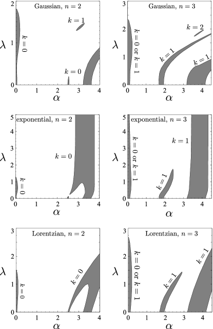
Figure 1: Linear limit stability diagrams for $n=2$ and $n=3$ in the plane $(\alpha,\lambda)$. Darker domains correspond to instability. Labels “$k=0$”, “$k=1$”, etc. at the unstable domains show the number of the double eigenvalue $\Omega_{n,k}$ responsible for the instability.

VII Nonlinear modes of finite amplitude

The stability results of the previous sections apply to nonlinear modes of infinitesimally small amplitude. One can check persistence of the stability results by constructing numerically the families of nonlinear modes of finite amplitude and computing the eigenvalues of the corresponding linear stability problem. The families of nonlinear modes can be visualized in the form of continuous curves on the plane $\sigma U$ vs. $b$ where $U=\int|w_{n}(x)|^{2}dx$ is the total energy flow. Then the small-amplitude modes are situated in the vicinity of the points $b_{n}=-(2n+1)$, $\sigma U=0$.

Let us first recall the results related to the local case ($\lambda=0$). The corresponding diagrams for the conservative case AlZez and for the ${\cal PT}$-symmetric case ZezKon12 are presented in the two upper panels of Fig. 2. The panels show several families that bifurcate from the lowest linear eigenvalues $n=0,1,2,3$. In the conservative case, only the two lowest families ($n=0,1$) are stable in the small-amplitude limit, whereas the small-amplitude modes with $n=2,3$ are unstable, In the ${\cal PT}$-symmetric case, all the four shown families are stable in the linear limit, but at least three of the four families loose stability as the strength of nonlinearity becomes sufficiently large.

The diagrams for the nonlocal case $\lambda=4$ (with the Gaussian kernel) are shown in the lower panels of Fig. 2. According to Table 1 and Fig. 1, at the chosen value of the nonlocality parameter, the nonlinear modes with $n=0,1,2,3$ are stable in the small-amplitude limit. The numerical results in Fig. 2 indicate that the stability persists at least for small and moderate strengths of the nonlinearity ($|\sigma U|\lesssim 40$). Notice also that in the panel with $(\alpha=1,\lambda=4)$ the nonlocality cancels the merging between the subsequent families which can be observed in the panel with $(\alpha=1,\lambda=0)$. We however emphasize that an accurate description of the limit of strong nonlinearity $|\sigma U|\to\infty$ should be elaborated by means of a proper asymptotic technique. While in the local case such studies have been already initiated CPK10 ; GP14 , analysis of the nonlocal ${\cal PT}$-symmetric case in the limit of strong nonlinearity remains the open issue at the moment.

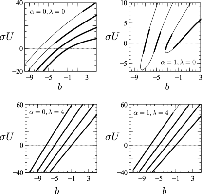
Figure 2: The families of nonlinear modes with $n=0,1,2,3$ for different $\alpha$ and $\lambda$ (the Gaussian kernel). Stable modes correspond to the bold fragments of the curves.

VIII Conclusion

In this study, we have demonstrated that the combined effect of the parabolic potential, nonlocality and ${\cal PT}$ symmetry results in a nontrivial stability picture for high-order small-amplitude nonlinear modes. The specific results of our work can be outlined as follows:

• A set of continuous families of nonlinear modes exists in the nonlocal ${\cal PT}$-symmetric nonlinear Schrödinger equation. The spectrum of the corresponding linear eigenvalue problem is available in the analytical form, and thus the stability problem for the small-amplitude nonlinear modes can be reduced to the searching real roots of certain analytical expressions.

• In the conservative case, small-amplitude nonlinear modes of arbitrary order become stable for sufficiently strong nonlocality, provided that the kernel is a sufficiently smooth function in the vicinity of the origin. If the kernel feature a singularity at $x=0$, no stabilization of high-order nonlinear modes is observed.

• Both the degree of nonlocality and the strength of the ${\cal PT}$ symmetry can be used to manage stability of the small-amplitude modes.

• The above stability conclusions remain valid for nonlinear modes of finite amplitude.

Appendix A Examples of expressions for $D_{n,k}$

Let us present expressions $D_{1,0}$ and $D_{2,0}$ computed for the Gaussian kernel and $\alpha=0$:

$$D_{1,0} = \displaystyle\frac{1}{4}\,{\frac{\left(2\,{\lambda}^{2}+1\right)^{2}}{\pi\left(\lambda^{2}+2\right)^{5}}},$$ (33)

$$D_{2,0} = {\frac{1}{64}}\,\frac{13968\,{{\lambda}}^{16}-28032\,{{\lambda}}^{14}-584\,{{\lambda}}^{12}-177136\,{{\lambda}}^{10}-54255\,{{\lambda}}^{8}-7564\,{{\lambda}}^{6}+4306\,{{\lambda}}^{4}-948\,{{\lambda}}^{2}-207}{\pi\,\left({{\lambda}}^{2}+2\right)^{13}}.$$ (34)

Obviously, $D_{1,0}$ is positive for any $\lambda$, while $D_{2,0}$ is negative for $\lambda=0$, but becomes positive for sufficiently large $\lambda$. Using the standard numerical tools for searching the roots of polynomials, we find that $D_{2,0}$ has two real zeros: $\lambda\approx\pm 1.82$. The positive one is presented in the respective row ($n=2$, $k=0$) of Table 1.

Appendix B Definition and some properties of the Fourier transform

We define the forward and backward Fourier transforms as

$$g(s)={\cal F}\{f\}=\int f(x)e^{isx}dx,$$ (35)

$$f(x)={\cal F}^{-1}\{g\}=\frac{1}{2\pi}\int g(s)e^{-isx}ds.$$ (36)

Then the Plancherel theorem says that

$$\int f_{1}(x)f_{2}^{*}(x)dx=\frac{1}{2\pi}\int g_{1}(s)g_{2}^{*}(s)ds,$$ (37)

where $g_{1,2}(s)={\cal F}\{f_{1,2}\}$; and from the convolution theorem one has

$${\cal F}\{h_{2}\}={\cal F}\{K\}{\cal F}\{h_{1}\},$$ (38)

where $h_{2}(x)=\int K(x-x^{\prime})h_{1}(x^{\prime})\ dx^{\prime}$.

Another well-known relation expresses the $p$th central moment of a function via the Fourier transform ($p=0,1,\ldots$):

$$\int x^{p}f(x)\ dx=(-i)^{p}\left.\frac{d^{p}}{ds^{p}}g(s)\right|_{s=0}.$$ (39)

Appendix C Some properties of the Hermite–Gauss eigenfunctions

Hereafter we assume the conservative case $\alpha=0$. The Hermite–Gauss eigenfunctions $\tilde{w}_{n}(x)$ are defined by Eqs. (8), see AS for definition of the Hermite and Laguerre polynomials. For $\alpha=0$ the modes $\tilde{w}_{n}(x)$ are real-valued and satisfy the normalization

$$\int_{-\infty}^{\infty}\tilde{w}_{n}^{2}(x)\ dx=1.$$ (40)

The eigenfunctions are mutually orthogonal, i.e., $\int\tilde{w}_{n}\tilde{w}_{k}\ dx=0$ for any $n$ and $k\neq n$. Moreover, for any $n$ and $k<n$:

$$\int x^{p}\tilde{w}_{n}(x)\,\tilde{w}_{k}(x)\ dx=0,\quad p=0,1,\ldots,n-k-1,$$ (41)

$$\int x^{n-k}\tilde{w}_{n}(x)\tilde{w}_{k}(x)\ dx=\sqrt{\frac{n!}{k!\,2^{n-k}}}.\quad\quad$$ (42)

In particular,

$$\int x\tilde{w}_{n}(x)\tilde{w}_{n-1}(x)\ dx=\sqrt{\frac{n}{2}}.$$ (43)

It is also useful to notice that

$$\int x^{2}\tilde{w}_{n}^{2}(x)\ dx=n+\frac{1}{2}.$$ (44)

Appendix D Asymptotics in the strongly nonlocal limit

We assume the conservative case $\alpha=0$ and an infinitely differentiable kernel written down as

$$K(x)=\frac{1}{\lambda}K_{0}\left(\frac{x}{\lambda}\right),$$ (45)

where function $K_{0}(x)$ is even, real, and infinitely differentiable for any $x$. Then one can adopt the Taylor series

$$K(x)=\sum_{p=0}^{\infty}\frac{K_{0}^{(p)}(0)x^{p}}{\lambda^{p+1}p!}.$$ (46)

For the sake of brevity, in what follows let us use the notation

$$F_{n,k}(s)={\cal F}\{\tilde{w}_{n}\tilde{w}_{k}\}=\int\tilde{w}_{n}(x)\tilde{w}_{k}(x)e^{isx}dx.$$ (47)

Asymptotics for $b_{n}^{(2)}$. We start from Eq. (11), use Eqs. (37), (38), (40), and (46), as well as reality of the function $F_{nn}(s)$, and evaluate $b_{n}^{(2)}$ as follows:

$$b_{n}^{(2)}=(2\pi)^{-1}\int{\cal F}\{K\}F_{n,n}^{2}(s)\ ds=$$

$$\int K(x){\cal F}^{-1}\{F^{2}_{n,n}(s)\}\ dx=$$

$$\sum_{p=0}^{\infty}\frac{K_{0}^{(p)}(0)}{\lambda^{p+1}p!}\int x^{p}{\cal F}^{-1}\{F_{n,n}^{2}(s)\}\ dx=$$

$$\sum_{p=0}^{\infty}\frac{K_{0}^{(p)}(0)}{\lambda^{p+1}p!}(-i)^{p}\left.\frac{d^{p}}{ds^{p}}F_{nn}^{2}(s)\right|_{s=0}$$

(in order to obtain the latter equality we also used (39)).

From the definition of $F_{n,n}(s)$ and from Eqs. (40)–(44), one can establish the following expansion:

$$F_{n,n}(s)=1-\frac{1}{2}\left(n+\frac{1}{2}\right)s^{2}+o(s^{2})_{s\to 0}.$$ (48)

Therefore

$$b_{n}^{(2)}=\frac{K_{0}(0)}{\lambda}+\frac{K^{\prime\prime}_{0}(0)(2n+1)}{2\lambda^{3}}+O(\lambda^{-4})_{\lambda\to+\infty}.$$ (49)

Asymptotics for $(M_{n,k})_{1,1}$. Since the asymptotics for $b_{n}^{(2)}$ is known from Eq. (49), it is convenient to consider the quantity $(M_{n,k})_{1,1}+b_{n}^{(2)}$ which can be evaluated as

$$\sum_{p=0}^{\infty}\frac{K_{0}^{(p)}(0)}{\lambda^{p+1}p!}(-i)^{p}\frac{d^{p}}{ds^{p}}\left(F_{n,n}(s)F_{k,k}(s)+|F_{n,k}(s)|^{2}\right)_{s=0}.$$

Using (48) and that

$$F_{n,k}(s)=is\int x\tilde{w}_{n}(x)\tilde{w}_{k}(x)\ dx+o(s)_{s\to 0},$$ (50)

one can find the resulting asymptotics

$$(M_{n,k})_{1,1}=-\frac{K^{\prime\prime}_{0}(0)\left(n-k+2(\int x\tilde{w}_{n}\tilde{w}_{k}\ dx)^{2}\right)}{2\lambda^{3}}$$

$$+O(\lambda^{-4})_{\lambda\to+\infty}.$$

The terms decaying as $\lambda^{-1}$ cancel each other.

For $k=0,1,\ldots,n-2$ one has $\int x\tilde{w}_{n}\tilde{w}_{k}\ dx=0$ and therefore

$$(M_{n,k})_{1,1}=-\frac{K^{\prime\prime}_{0}(0)(n-k)}{2\lambda^{3}}+O(\lambda^{-4})_{\lambda\to+\infty},$$

while for $k=n-1$ one can use Eq. (43) and obtain

$$(M_{n,n-1})_{1,1}=-\frac{K^{\prime\prime}_{0}(0)(n+1)}{2\lambda^{3}}+O(\lambda^{-4})_{\lambda\to+\infty}.$$

Asymptotics for $(M_{n,k})_{2,1}$. Following to the same ideas, we can write down

$$(M_{n,k})_{2,1}=-\sum_{p=0}^{\infty}\frac{K_{0}^{(p)}(0)}{\lambda^{p+1}p!}(-i)^{p}\frac{d^{p}}{ds^{p}}\left(F_{n,2n-k}(s)F_{n,k}^{*}(s)\right)_{s=0}.$$ (51)

From definition of functions $F_{n,k}(s)$ and $F_{n,2n-k}(s)$ it follows that in vicinity of $s=0$ they behave as

$$F_{n,k}(s)=\frac{i^{n-k}}{(n-k)!}\sqrt{\frac{n!}{k!\,2^{n-k}}}\ s^{n-k}+o(s^{n-k})_{s\to 0},$$

$$F_{2n-k,k}(s)=\frac{i^{n-k}}{(n-k)!}\sqrt{\frac{(2n-k)!}{n!\,2^{n-k}}}\ s^{n-k}+o(s^{n-k})_{s\to 0}.$$

Therefore several first terms of the series (51) are zero, and the first nonzero term corresponds to $p=2(n-k)$ (provided that $K_{0}^{(2n-2k)}(0)\neq 0$). Specifically,

$$(M_{n,k})_{2,1}=\frac{(-1)^{n-k+1}K^{(2n-2k)}_{0}(0)}{2^{n-k}((n-k)!)^{2}\lambda^{2n-2k+1}}\sqrt{\frac{(2n-k)!}{k!}}$$

$$+O\left(\frac{1}{\lambda^{2n-2k+2}}\right)_{\lambda\to+\infty}.$$

Finally we notice that proceeding in exactly the same way, one can prove analogous behavior of the other two entries $M_{n,k}$. Namely, $(M_{n,k})_{2,2}$ decays as $\lambda^{-3}$, while $(M_{n,k})_{1,2}$ decays as $\lambda^{-(2n-2k+1)}$ for $\lambda\to\infty$.

- (1) A. G. Litvak, JETF Lett. 4, 230 (1966).
- (2) A. C. Tam and W. Happer, Phys. Rev. Lett. 38, 278 (1977); D. Suter and T. Blasberg, Phys. Rev. A 48, 4583 (1993).
- (3) S. K. Turitsyn, Theor. Math. Phys. (Engl. Transl.) 64, 797 (1985).
- (4) W. Krolikowski and O. Bang, Phys. Rev. E 63, 016610 (2000).
- (5) Z. Xu, Y. V. Kartashov, and L. Torner, Opt. Lett 30, 3171 (2005).
- (6) S. Skupin, O. Bang, D. Edmundson, and W. Krolikowski, Phys. Rev. E 73, 066603 (2006).
- (7) O. Bang, W. Krolikowski, J. Wyller, and J. J. Rasmussen, Phys. Rev. E 66, 046619 (2002).
- (8) A. Dreischuh, D. N. Neshev, D. E. Petersen, O. Bang, and W. Krolikowski, Phys. Rev. Lett. 96, 043901 (2006).
- (9) L. P. Pitaevskii and S. Stringari, Bose-Einstein Condensation (Clarendon Press: Oxford and New York, 2003).
- (10) K. Góral, K. Rza̧żewski, and T. Pfau, Phys. Rev. A 61, 051601(R) (2000); S. Yi and L. You, ibid. 041604(R); L. Santos, G. V. Shlyapnikov, P. Zoller, and M. Lewenstein, Phys. Rev. Lett. 85 1791 (2000); P. Pedri and L. Santos, ibid. 95, 200404 (2005);
- (11) S. Sinha and L. Santos, Phys. Rev. Lett. 99, 140406 (2007).
- (12) A. G. Litvak and A. M. Sergeev, JETP Lett. 27, 517 (1978).
- (13) C. Conti, M. Peccianti, and G. Assanto, Phys. Rev. Lett. 91, 073901 (2003); ibid. 92, 113902 (2004).
- (14) M. Kunze, T. Küpper, V.K. Mezentsev, E. G. Shapiro, and S. Turitsyn, Physica D 128, 273 (1999); Yu. S. Kivshar, T. Alexander, and S. K. Turitsyn, 2001, Phys. Lett. A 278, 225; V. I. Yukalov, E. P. Yukalova, and V. S. Bagnato, Phys. Rev. A 66, 043602 (2002); R. D’ Agosta, B. A. Malomed, and C. Presilla, Laser Phys. 12, 37 (2002); V. V. Konotop and P. G. Kevrekidis, Phys. Rev. Lett. 91, 230402 (2003); P. G. Kevrekidis, V. V. Konotop, A. Rodrigues, and D. J. Frantzeskakis, J. Phys. B: At. Mol. Opt. Phys. 38, 1173 (2005).
- (15) M. Edwards, K. Burnett, Phys. Rev. A 51, 1382 (1995); P. A. Ruprecht, M. J. Holland, K. Burnett, and M. Edwards, Phys. Rev. A 51, 4704 (1995); F. Dalfovo and S. Stringari, Phys. Rev. A 53, 2477 (1996); V. I. Yukalov, E. P. Yukalova, and V. S. Bagnato, Phys. Rev. A 56, 4845 (1997).
- (16) C. Wang, P. G. Kevrekidis, D. J. Frantzeskakis, B. A. Malomed, Physica D 240 805 (2011); P. A. Tsilifis, P. G. Kevrekidis, and V. M. Rothos, J. Phys. A: Math. Theor. 47, 035201 (2014).
- (17) Y. V. Kartashov, V. A. Vysloukh, and L. Torner, Phys. Rev. Lett. 93, 153903 (2004).
- (18) Z. Xu, Y. V. Kartashov, and L. Torner, Phys. Rev. Lett. 95, 113901 (2005); N. K. Efremidis, Phys. Rev. A 77, 063824 (2008).
- (19) J. Cuevas, B. A. Malomed, P. G. Kevrekidis, and D. J. Frantzeskakis, Phys. Rev. A 79, 053608 (2009).
- (20) D. A. Zezyulin, G. L. Alfimov, V. V. Konotop, and V. M. Pérez-García, Phys. Rev. A 78, 013606 (2008).
- (21) C. M. Bender, and S. Boettcher, Phys. Rev. Lett. 80, 5243 (1998).
- (22) C. E. Rüter, K. G. Makris, R. El-Ganainy, D. N. Christodoulides, M. Segev, and D. Kip, Nat. Phys. 6, 192 (2010).
- (23) C. Hang, G. Huang, and V. V. Konotop, Phys. Rev. Lett. 110, 083604 (2013); C. Hang, D. A. Zezyulin, V. V. Konotop, and G. Huang, Opt. Lett. 38, 4033 (2013); C. Hang, D. A. Zezyulin, G. Huang, V. V. Konotop, and B. A. Malomed, ibid. 39, 5387 (2014).
- (24) S. Klaiman, U. Günther, and N. Moiseyev, Phys. Rev. Lett. 101, 080402 (2008).
- (25) Z. H. Musslimani, K. G. Makris, R. El-Ganainy, and D. N. Christodoulides, Phys. Rev. Lett. 100, 030402 (2008).
- (26) Sumei Hu, Xuekai Ma, Daquan Lu, Zhenjun Yang, Yizhou Zheng, and Wei Hu, Phys. Rev. A 84, 043818 (2011); Zhiwei Shi, Xiujuan Jiang, Xing Zhu, and Huagang Li, Phys. Rev. A 84, 053855 (2011); S. Nixon, L. Ge, and J. Yang, Phys. Rev. A 85, 023822 (2012); V. Achilleos, P. G. Kevrekidis, D. J. Frantzeskakis, and R. Carretero-González, Phys. Rev. A 86, 013808 (2012); X. Zhu, H. Wang, L. X. Zheng, H. Li, and Y. J. He, Opt. Lett. 36, 2680 (2011); Keya Zhou, Zhongyi Guo, Jicheng Wang, and Shutian Liu, Opt. Lett. 35, 2928 (2010); H. Wang and J. Wang, Opt. Express 19, 4030 (2011); Zhien Lu and Zhi-Ming Zhang, ibid. 19, 11457 (2011).
- (27) D. A. Zezyulin and V. V. Konotop, Phys. Rev. A 85, 043840 (2012).
- (28) Z. H. Shi, H. Li, X. Zhu, and X. Jiang, EPL 98, 64006 (2012); S. Hu, D. Lu, X. Ma, Q. Guo, and W. Hu, EPL 98, 14006 (2012); X. Zhu, H. Li, H. Wang, and Y. He, JOSA B 30, 1987 (2013); S. Hu, X. Ma, D. Lu, Y. Zheng, and W. Hu, Phys. Rev. A ibid., 043826 (2012) H. Li, X. Jiang, X. Zhu, and Z. Shi, Phys. Rev. A 86, 023840 (2012); C. P. Jisha, A. Alberucci, V. A. Brazhnyi, and G. Assanto, ibid. 89, 013812 (2014); L. Fang, J. Gao, Z. Shi, X. Zhu, and H. Li, Eur. Phys. J. D 68, 298 (2014);
- (29) V. M. Pérez-García, V. V. Konotop, and J. J. García-Ripoll, Phys. Rev. E 62, 4300 (2000); J. J. García-Ripoll, V. V. Konotop, B. Malomed, and V. M. Pérez-García Mathematics and Computers in Simulation 62, 21-30 (2003).
- (30) T. Kato, Perturbation Theory for Linear Operators (Springer-Verlag, Berlin, 1966).
- (31) M. Znojil, Phys. Lett. A 259, 220 (1999).
- (32) Handbook of Mathematical Functions, edited by M. Abramovitz and I. A. Stegun (National Bureau of Standards, Washington, DC, 1972).
- (33) T. Dohnal and P. Siegl, Bifurcation of nonlinear eigenvalues in problems with antilinear symmetry, arXiv:1504.00054 [math-ph].
- (34) M. P. Coles, D. E. Pelinovsky, and P. G. Kevrekidis, Nonlinearity 23, 1753 (2010).
- (35) C. Gallo and D. Pelinovsky, Stud. App. Math. 133, 398 (2014).