A path property of Dyson gaps,
Plancherel measures for Sโ€‹pโ€‹(โˆž)๐‘†๐‘Sp(\infty),
and random surface growth

Mark Cerenzia
Princeton University
Electronic address: cerenzia@princeton.edu
Abstract

We pursue applications for symplectic Plancherel growth based on a repulsion phenomenon arising in its diffusion limit and on intermediate representation theory underlying its correlation structure. Under diffusive scaling, the dynamics converge to interlaced reflecting Brownian motions with a wall that achieve Dyson non-colliding dynamics. We exhibit non-degeneracy of constraint in this coupled system by deriving a path property that quantifies repulsion between particles coinciding in the limit. We then identify consistent series of Plancherel measures for Sโ€‹pโ€‹(โˆž)๐‘†๐‘Sp(\infty) that reflect the odd symplectic groups, despite their non-semisimplicity. As an application, we compute the correlation kernel of the growth model and investigate its local asymptotics: the incomplete beta kernel emerges in the bulk limit, and new variants of the Jacobi and Pearcey kernels arise as edge limits. In particular, we provide further evidence for the universality of the 1/4141/4-growth exponent and Pearcey point process in the class of anisotropic KPZ with a wall.

1 Introduction

Plancherel growth processes are certain continuous dynamics for Gelfand-Tsetlin patterns that can serve as prototypes for studying probabilistic phenomena in systems involving short-range dependence and simple interactions (for us, blocking and pushing). Figure 1 depicts an instance of the dynamics studied in this paper.

Refer to caption
Refer to caption
Refer to caption
Refer to caption
Figure 1: Three possible initial steps of either orthogonal or symplectic Plancherel growth. The arrows indicate the direction that the particle will attempt to jump next; see Figure 2 for the fourth step. The tiling determined by their positions suggests a stepped-surface interpretation.
Refer to caption
Refer to caption
Refer to caption
Refer to caption
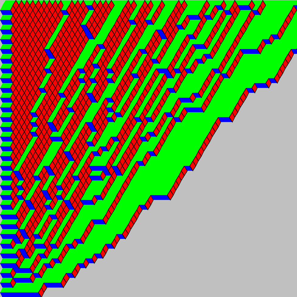
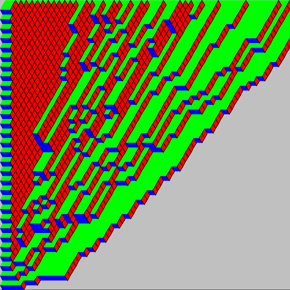
Figure 2: The fourth step illustrates the distinctive wall behaviors: reflection (left) and suppression (right). Simulations of the orthogonal and symplectic cases indicate similar average behavior.

In our orthogonal/symplectic patterns, level nโˆˆโ„ค>0:={1,2,3โ€‹โ€ฆ}๐‘›subscriptโ„คabsent0assign123โ€ฆn\in\mathbb{Z}_{>0}:=\{1,2,3\ldots\} has rn:=โŒŠ(n+1)/2โŒ‹assignsubscript๐‘Ÿ๐‘›๐‘›12r_{n}:=\lfloor(n+1)/2\rfloor particles yinsubscriptsuperscript๐‘ฆ๐‘›๐‘–y^{n}_{i}, 1โ‰คiโ‰คrn1๐‘–subscript๐‘Ÿ๐‘›1\leq i\leq r_{n}, in โ„คโ‰ฅ0:={0,1,2,โ€ฆ}assignsubscriptโ„คabsent0012โ€ฆ\mathbb{Z}_{\geq 0}:=\{0,1,2,\ldots\}. Symplectic Plancherel growth features these particles performing independent simple random walks, but a unit jump of a particle yinsubscriptsuperscript๐‘ฆ๐‘›๐‘–y^{n}_{i} is suppressed or forced if otherwise it would land outside of the interval (write y0nโˆ’1โ‰กโˆžsubscriptsuperscript๐‘ฆ๐‘›10y^{n-1}_{0}\equiv\infty)

{[0,yiโˆ’1nโˆ’1),i=rnโ€‹withโ€‹nโ‰ฅ1โ€‹odd(yinโˆ’1,yiโˆ’1nโˆ’1),otherwise forย 1โ‰คiโ‰คrn.cases0subscriptsuperscript๐‘ฆ๐‘›1๐‘–1๐‘–subscript๐‘Ÿ๐‘›with๐‘›1oddsubscriptsuperscript๐‘ฆ๐‘›1๐‘–subscriptsuperscript๐‘ฆ๐‘›1๐‘–1otherwise forย 1โ‰คiโ‰คrn\begin{cases}\left[0,y^{n-1}_{i-1}\right),&i=r_{n}\ \text{with}\ n\geq 1\ \text{odd}\\ \left(y^{n-1}_{i},y^{n-1}_{i-1}\right),&\text{otherwise for $1\leq i\leq r_{n}$}\\ \end{cases}.

In particular, the โ€œwall-particlesโ€ yrnnsubscriptsuperscript๐‘ฆ๐‘›subscript๐‘Ÿ๐‘›y^{n}_{r_{n}} at odd levels nโ‰ฅ1๐‘›1n\geq 1 are ๐ฌ๐ฎ๐ฉ๐ฉ๐ซ๐ž๐ฌ๐ฌ๐ž๐๐ฌ๐ฎ๐ฉ๐ฉ๐ซ๐ž๐ฌ๐ฌ๐ž๐\mathbf{suppressed} by the wall at 00. This blocking and pushing of a particle by straddling particles on the previous level (including 00 and โˆž\infty) serves to maintain interlacing conditions, which in the chosen coordinates read as

{0โ‰คyin<yin+1,i=rnโ€‹withโ€‹nโ‰ฅ1โ€‹oddyi+1n+1<yin<yin+1,otherwise forย 1โ‰คiโ‰คrn.cases0subscriptsuperscript๐‘ฆ๐‘›๐‘–subscriptsuperscript๐‘ฆ๐‘›1๐‘–๐‘–subscript๐‘Ÿ๐‘›with๐‘›1oddsubscriptsuperscript๐‘ฆ๐‘›1๐‘–1subscriptsuperscript๐‘ฆ๐‘›๐‘–subscriptsuperscript๐‘ฆ๐‘›1๐‘–otherwise forย 1โ‰คiโ‰คrn\begin{cases}0\leq y^{n}_{i}<y^{n+1}_{i},&i=r_{n}\ \text{with}\ n\geq 1\ \text{odd}\\ y^{n+1}_{i+1}<y^{n}_{i}<y^{n+1}_{i},&\text{otherwise for $1\leq i\leq r_{n}$}\end{cases}. (1)

Orthogonal Plancherel growth studied by Borodinโ€“Kuan [14] differs only by the ๐ซ๐ž๐Ÿ๐ฅ๐ž๐œ๐ญ๐ข๐จ๐ง๐ซ๐ž๐Ÿ๐ฅ๐ž๐œ๐ญ๐ข๐จ๐ง\mathbf{reflection} of jumps into the wall at 00. Although the difference between the two systems may seem negligible at first, note that a single wall-particleโ€™s movement can cause the models to diverge by infinitely many particle positions; see Figure 2 for a comparison. Since local limit behavior of such integrable probability models can be sensitive to their basic parameters (notably, to initial conditions; see, e.g., [11]), it is worth investigating to what degree the distinct wall behavior is felt in the correlation structure and in various asymptotic regimes. To explain terminology, when deriving these dynamics via representation theory, the wall behavior originates from the initial conditions of orthogonal polynomials used to express irreducible/indecomposable characters of even-orthogonal/odd-symplectic groups; see Section 5.3. This remark indicates another, a priori significant departure from the orthogonal case: the relevance of the representation theory of non-semisimple Lie groups intermediate in the classical symplectic series. For readers less familiar with these algebraic items, note that all necessary concepts are reviewed and that Section 2 relies only on modern probability theory.

1.1 Main goals and motivation

We have two primary goals:

  1. 1.

    To quantify repulsion in the Dyson non-colliding dynamics achieved in the diffusion limit in order to exhibit non-degeneracy of constraint in this regime.

  2. 2.

    To compute series of Plancherel measures for Sโ€‹pโ€‹(โˆž)๐‘†๐‘Sp(\infty) that reflect the intermediate representation theory of the non-semisimple odd symplectic groups, and subsequently investigate their role in the correlation structure and local limit behavior of symplectic Plancherel growth.

In pursuing the first goal, we resolve a basic version of the conjecture posed after Proposition 2 of [12], confirm the decompositions (4),(29)429(4),(29) in [47] when the interlaced system starts at the origin, and thus also lift the restriction in [27] that the limiting system must start in the interior of the chamber. To show that the amount of constraint in the pre-limit system does not degenerate in this regime, we need to quantify the repulsion between particles coinciding in the limit. The path property that assumes this role is interesting in its own right: it delineates a lower envelope at t=0๐‘ก0t=0 for a multivariate self-similar process with positive components that do not drift to infinity almost surely. For such โ„+subscriptโ„\mathbb{R}_{+}-valued Markov processes drifting to infinity, see [21] for rather general techniques and integral tests. The results of Section 2.4 at the heart of this development are new in this literature and are inspired by Burdzyโ€“Kangโ€“Ramanan [20]; we otherwise briskly follow the elegant procedures of Gorin-Shkolnikov [27] and Warren [47]. For the related case of vicious random walkers, see the series of results by Katori, Tanemura, et.al., whose paper [31] covers convergence of our even levels.

For the second goal, the non-semisimplicity of odd symplectic groups is a potentially serious obstacle for the identification of suitable โ€œintermediateโ€ Plancherel measures for Sโ€‹pโ€‹(โˆž)๐‘†๐‘Sp(\infty) โ€“ such measures can no longer arise as coefficients of irreducible characters in the orthogonal decomposition of restricted infinite extreme characters. Circumventing this lack of irreducibility relies on the independent works of Proctor [41] and Shtepin [43], and we suspect there are more connections in this vein to be made between probability theory and nonclassical representation theoretic objects. Defosseux [23] and Warrenโ€“Windridge [48] have already considered our dynamics for symplectic Gelfand-Tsetlin patterns, with the latter paper anticipating our interest, but the results we derive here are much in the same spirit as Borodinโ€“Kuan [14], who cover the orthogonal case. Obtaining refined local limit behavior in their manner is well codified, originating with a law of large numbers result for the limit shape of random Young tableaux, derived independently by Vershikโ€“Kerov [46] and Loganโ€“Shepp [37]. The former pair were studying asymptotics of the maximum dimension of irreducible representations for the symmetric group, and the latter were pursuing a variational problem arising in combinatorics posed by Richard Stanley. Baikโ€“Deiftโ€“Johansson [3], and shortly after Okounkov [38], derived more detailed results concerning local behavior at the edge of the limit shape, inspiring much research on such behavior, including the present work; for a perfunctory list, consider [3, 6, 7, 8, 9, 10, 11, 13, 14, 15, 16, 17, 34, 35, 37, 38, 39, 40, 46].

Important Notational Convention.

Quantities with indices that overflow are set to 00 and those with indices that underflow are set to โˆž\infty.

1.2 Main applications

1.2.1 Diffusive scaling limit: non-degeneracy of constrained dynamics

The basic description of symplectic Plancherel growth (considered up to level nโ‰ฅ1๐‘›1n\geq 1) readily leads to the candidate diffusive limiting system (๐’ฒโ€‹(t))tโ‰ฅ0subscript๐’ฒ๐‘ก๐‘ก0(\mathcal{W}(t))_{t\geq 0} with components ๐’ฒiksubscriptsuperscript๐’ฒ๐‘˜๐‘–\mathcal{W}^{k}_{i} satisfying

๐’ฒikโ€‹is a Brownian motionย Bikย reflected in the intervalโ€‹{[0,โˆž),ifโ€‹k=1[๐’ฒikโˆ’1,๐’ฒiโˆ’1kโˆ’1],ifโ€‹kโ‰ฅ2subscriptsuperscript๐’ฒ๐‘˜๐‘–is a Brownian motionย Bikย reflected in the intervalcases0if๐‘˜1subscriptsuperscript๐’ฒ๐‘˜1๐‘–subscriptsuperscript๐’ฒ๐‘˜1๐‘–1if๐‘˜2\mathcal{W}^{k}_{i}\ \text{is a Brownian motion $B_{i}^{k}$ reflected in the interval}\ \begin{cases}[0,\infty),&\ \ \text{if}\ k=1\\ [\mathcal{W}^{k-1}_{i},\mathcal{W}^{k-1}_{i-1}],&\ \ \text{if}\ k\geq 2\end{cases} (2)

for 1โ‰คkโ‰คn1๐‘˜๐‘›1\leq k\leq n, 1โ‰คiโ‰คrk1๐‘–subscript๐‘Ÿ๐‘˜1\leq i\leq r_{k}, where the Biksubscriptsuperscript๐ต๐‘˜๐‘–B^{k}_{i} are independent and started at 00; note our notational convention puts additional static particles at 00 (for index overflow) and at โˆž\infty (for index underflow). Section 2.1 makes the notion of reflecting Brownian movements in a time-dependent domain rigorous, but we say the coupled dynamics of (๐’ฒโ€‹(t))tโ‰ฅ0subscript๐’ฒ๐‘ก๐‘ก0(\mathcal{W}(t))_{t\geq 0} are non-degenerate if its components uniquely solve the system of equations

๐’ฒik={Bik+12โ€‹L๐’ฒik0โˆ’L(๐’ฒiโˆ’1kโˆ’1โˆ’๐’ฒik)0,i=rkโ€‹withโ€‹kโ€‹oddBik+L(๐’ฒikโˆ’๐’ฒikโˆ’1)0โˆ’L(๐’ฒiโˆ’1kโˆ’1โˆ’๐’ฒik)0,otherwise forโ€‹ 1โ‰คiโ‰คrk,subscriptsuperscript๐’ฒ๐‘˜๐‘–casessuperscriptsubscript๐ต๐‘–๐‘˜12subscriptsuperscript๐ฟ0subscriptsuperscript๐’ฒ๐‘˜๐‘–subscriptsuperscript๐ฟ0subscriptsuperscript๐’ฒ๐‘˜1๐‘–1subscriptsuperscript๐’ฒ๐‘˜๐‘–๐‘–subscript๐‘Ÿ๐‘˜with๐‘˜oddsuperscriptsubscript๐ต๐‘–๐‘˜subscriptsuperscript๐ฟ0subscriptsuperscript๐’ฒ๐‘˜๐‘–subscriptsuperscript๐’ฒ๐‘˜1๐‘–subscriptsuperscript๐ฟ0subscriptsuperscript๐’ฒ๐‘˜1๐‘–1subscriptsuperscript๐’ฒ๐‘˜๐‘–otherwise for1๐‘–subscript๐‘Ÿ๐‘˜\mathcal{W}^{k}_{i}=\begin{cases}B_{i}^{k}+\frac{1}{2}L^{0}_{\mathcal{W}^{k}_{i}}-L^{0}_{(\mathcal{W}^{k-1}_{i-1}-\mathcal{W}^{k}_{i})},&i=r_{k}\ \text{with}\ k\ \text{odd}\\ B_{i}^{k}+L^{0}_{(\mathcal{W}^{k}_{i}-\mathcal{W}^{k-1}_{i})}-L^{0}_{(\mathcal{W}^{k-1}_{i-1}-\mathcal{W}^{k}_{i})},&\text{otherwise for}\ 1\leq i\leq r_{k}\end{cases}, (3)

where LY0superscriptsubscript๐ฟ๐‘Œ0L_{Y}^{0} is twice the semimartingale local time at 00 of a semimartingale Y๐‘ŒY and where Lโˆž0โ‰ก0subscriptsuperscript๐ฟ00L^{0}_{\infty}\equiv 0 (see Remark 4.2 of [20] for an explanation of the appropriate local time scalings). Intuitively, these equations indicate the amount of constraint in the system (๐’ฒโ€‹(t))0โ‰คtโ‰คTsubscript๐’ฒ๐‘ก0๐‘ก๐‘‡(\mathcal{W}(t))_{0\leq t\leq T} is finite for every Tโ‰ฅ0๐‘‡0T\geq 0. But demonstrating non-degeneracy of (๐’ฒโ€‹(t))tโ‰ฅ0subscript๐’ฒ๐‘ก๐‘ก0(\mathcal{W}(t))_{t\geq 0} requires that we resolve a subtle yet concrete difficulty.
Refer to caption
Refer to caption
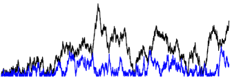
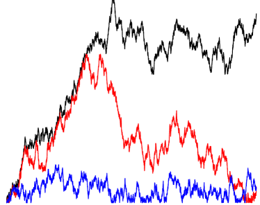
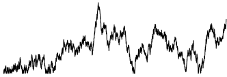
Figure 3: The first path in black is a standard brownian motion reflected at 00. Reflecting the blue path to stay between 00 and the black path requires an โ€œinfinite amountโ€ of constraining to achieve.
Refer to caption
Refer to caption
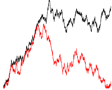
Figure 4: Diffusion limit of first three particles nearest the wall (visualized in the single state space โ„+subscriptโ„\mathbb{R}_{+}). The level 1 particle in red creates a repulsion between the wall at 00 and the level 2 particle in black; although this extra room may still not be enough, we show the reflected level 3 wall-particle in blue has non-degenerate constrained dynamics.

To see the issue in our case, write the dynamics of a typical reflected particle in the basic decomposition W=B+Y๐‘Š๐ต๐‘ŒW=B+Y, where the constraining process Y๐‘ŒY โ€œpushesโ€ the Brownian particle B๐ตB to remain between some independent particles โ„“,rโ„“๐‘Ÿ\ell,r on the previous level. If ever the interval [โ„“โ€‹(t),rโ€‹(t)]โ„“๐‘ก๐‘Ÿ๐‘ก[\ell(t),r(t)] collapses, Y๐‘ŒY might need to โ€œpush an infinite amountโ€ in order to keep B๐ตB at that point. For example, Y๐‘ŒY can be finite variation on every period between collapse times of [โ„“โ€‹(t),rโ€‹(t)]โ„“๐‘ก๐‘Ÿ๐‘ก[\ell(t),r(t)], but accumulate infinite variation over infinitely many such periods in finite time; see Figure 3 for such a scenario.

For a more surprising and relevant example, the interval [โ„“โ€‹(t),rโ€‹(t)]โ„“๐‘ก๐‘Ÿ๐‘ก[\ell(t),r(t)] can โ€œclose too quicklyโ€ at t=0๐‘ก0t=0, say, for some c>1๐‘1c>1, almost surely

lim suptโ†“0rโ€‹(t)โˆ’โ„“โ€‹(t)tc=0;subscriptlimit-supremumโ†“๐‘ก0๐‘Ÿ๐‘กโ„“๐‘กsuperscript๐‘ก๐‘0\limsup_{t\downarrow 0}\frac{r(t)-\ell(t)}{t^{c}}=0; (4)

in this situation, even if the particles โ„“โ€‹(t),rโ€‹(t)โ„“๐‘ก๐‘Ÿ๐‘ก\ell(t),r(t) remain apart for t>0๐‘ก0t>0, Y๐‘ŒY will not be of bounded variation. If Y๐‘ŒY is of infinite variation, then the symbols indicating local times in (3) do not make sense (even though their increments may). Proposition 4.13 and the proof of Proposition 4.12 of [20] provide more details on these two degenerate examples.

Fortunately, by the construction of our system (2), any particles โ„“,rโ„“๐‘Ÿ\ell,r that can collide must straddle an independent Brownian particle on a further previous level that could create a sufficiently strong repulsion that Y๐‘ŒY only needs to โ€œpush a finite amountโ€ to keep B๐ตB between them; see Figure 4. Our strategy, then, consists of quantifying this degree of repulsion in order to rule out the degenerate possibility (4) and exhibit non-degeneracy of the constrained dynamics (๐’ฒโ€‹(t))tโ‰ฅ0subscript๐’ฒ๐‘ก๐‘ก0(\mathcal{W}(t))_{t\geq 0} of (2). More broadly, Section 2 will establish the following result.

Theorem 1.1.

Fix nโ‰ฅ1๐‘›1n\geq 1. The interlaced system (๐’ฒโ€‹(t))tโ‰ฅ0subscript๐’ฒ๐‘ก๐‘ก0(\mathcal{W}(t))_{t\geq 0} of reflecting Brownian motions with a wall defined by (2) has levels ๐’ฒksuperscript๐’ฒ๐‘˜\mathcal{W}^{k}, 1โ‰คkโ‰คn1๐‘˜๐‘›1\leq k\leq n, that achieve the Dyson non-colliding dynamics

dโ€‹Xik={dโ€‹Bi+dโ€‹tXik+โˆ‘jโ‰ i1โ‰คjโ‰คrk(1Xikโˆ’Xjk+1Xik+Xjk)โ€‹dโ€‹t,ifkevendโ€‹Bi+12โ€‹1(i=rk)โ€‹dโ€‹LXik0โ€‹(t)+โˆ‘jโ‰ i1โ‰คjโ‰คrk(1Xikโˆ’Xjk+1Xik+Xjk)โ€‹dโ€‹t,ifkodd,๐‘‘subscriptsuperscript๐‘‹๐‘˜๐‘–cases๐‘‘subscript๐ต๐‘–๐‘‘๐‘กsubscriptsuperscript๐‘‹๐‘˜๐‘–subscript๐‘—๐‘–1๐‘—subscript๐‘Ÿ๐‘˜1superscriptsubscript๐‘‹๐‘–๐‘˜superscriptsubscript๐‘‹๐‘—๐‘˜1superscriptsubscript๐‘‹๐‘–๐‘˜superscriptsubscript๐‘‹๐‘—๐‘˜๐‘‘๐‘กif๐‘˜even๐‘‘subscript๐ต๐‘–12subscript1๐‘–subscript๐‘Ÿ๐‘˜๐‘‘superscriptsubscript๐ฟsubscriptsuperscript๐‘‹๐‘˜๐‘–0๐‘กsubscript๐‘—๐‘–1๐‘—subscript๐‘Ÿ๐‘˜1superscriptsubscript๐‘‹๐‘–๐‘˜superscriptsubscript๐‘‹๐‘—๐‘˜1superscriptsubscript๐‘‹๐‘–๐‘˜superscriptsubscript๐‘‹๐‘—๐‘˜๐‘‘๐‘กif๐‘˜odddX^{k}_{i}=\begin{cases}dB_{i}+\frac{dt}{X^{k}_{i}}+\sum_{\begin{subarray}{c}j\neq i\\ 1\leq j\leq r_{k}\end{subarray}}\left(\frac{1}{X_{i}^{k}-X_{j}^{k}}+\frac{1}{X_{i}^{k}+X_{j}^{k}}\right)dt,&\text{if}\ \ k\ \ \text{even}\\ dB_{i}+\frac{1}{2}1_{(i=r_{k})}dL_{X^{k}_{i}}^{0}(t)+\sum_{\begin{subarray}{c}j\neq i\\ 1\leq j\leq r_{k}\end{subarray}}\left(\frac{1}{X_{i}^{k}-X_{j}^{k}}+\frac{1}{X_{i}^{k}+X_{j}^{k}}\right)dt,&\text{if}\ \ k\ \ \text{odd}\end{cases}, (5)

for 1โ‰คiโ‰คrk1๐‘–subscript๐‘Ÿ๐‘˜1\leq i\leq r_{k}, where the Bisubscript๐ต๐‘–B_{i} are independent standard Brownian motions. Moreover, each particle ๐’ฒik+1subscriptsuperscript๐’ฒ๐‘˜1๐‘–\mathcal{W}^{k+1}_{i}, 2โ‰คk<n2๐‘˜๐‘›2\leq k<n, 1<iโ‰คrk+11๐‘–subscript๐‘Ÿ๐‘˜11<i\leq r_{k+1} is reflected in an interval [๐’ฒikโ€‹(t),๐’ฒiโˆ’1kโ€‹(t)]subscriptsuperscript๐’ฒ๐‘˜๐‘–๐‘กsubscriptsuperscript๐’ฒ๐‘˜๐‘–1๐‘ก[\mathcal{W}^{k}_{i}(t),\mathcal{W}^{k}_{i-1}(t)] satisfying the almost sure path property

lim inftโ†“0๐’ฒiโˆ’1kโ€‹(t)โˆ’๐’ฒikโ€‹(t)tc=โˆžsubscriptlimit-infimumโ†“๐‘ก0subscriptsuperscript๐’ฒ๐‘˜๐‘–1๐‘กsubscriptsuperscript๐’ฒ๐‘˜๐‘–๐‘กsuperscript๐‘ก๐‘\liminf_{t\downarrow 0}\frac{\mathcal{W}^{k}_{i-1}(t)-\mathcal{W}^{k}_{i}(t)}{t^{c}}=\infty

for any c>1/2๐‘12c>1/2; (๐’ฒโ€‹(t))tโ‰ฅ0subscript๐’ฒ๐‘ก๐‘ก0(\mathcal{W}(t))_{t\geq 0} is then verifiably the unique, strong solution to (3) when started at the origin. Hence, under diffusive space-time scaling, symplectic Plancherel growth considered up to level n๐‘›n converges in law to the non-degenerate system (3).

The path property above is readily seen to hold in Warrenโ€™s setting [47] of interlaced reflecting Brownian motions (without a wall), which achieve classical Dyson dynamics

dโ€‹ฮปti=dโ€‹Bti+ฮบ2โ€‹โˆ‘jโ‰ idโ€‹tฮปtiโˆ’ฮปtj, 1โ‰คiโ‰คN,formulae-sequence๐‘‘subscriptsuperscript๐œ†๐‘–๐‘ก๐‘‘subscriptsuperscript๐ต๐‘–๐‘ก๐œ…2subscript๐‘—๐‘–๐‘‘๐‘กsubscriptsuperscript๐œ†๐‘–๐‘กsubscriptsuperscript๐œ†๐‘—๐‘ก1๐‘–๐‘d\lambda^{i}_{t}=dB^{i}_{t}+\frac{\kappa}{2}\sum_{j\neq i}\frac{dt}{\lambda^{i}_{t}-\lambda^{j}_{t}},\ \ \ 1\leq i\leq N, (6)

where the Bisuperscript๐ต๐‘–B^{i} are independent. In particular, setting ฮบ=2๐œ…2\kappa=2 and arguing as in Section 2.4 confirms the decompositions (4),(29)429(4),(29) in [47] when the system starts at the origin and thus also lifts the restriction in [27] that the limiting system must start in the interior of the chamber {x1โ‰ฅโ€ฆโ‰ฅxN}subscript๐‘ฅ1โ€ฆsubscript๐‘ฅ๐‘\{x_{1}\geq\ldots\geq x_{N}\}. Note the path property for (6) is compelling only for Nโ‰ฅ3๐‘3N\geq 3; in the case N=2๐‘2N=2, the single gap is proportional to a 333-dimensional Bessel process and the result is classical.

1.2.2 Determinantal correlation kernel and local limit behavior

As we saw in the last section, the diffusion limit primarily cares inductively about interactions of three successive levels at a time. To capture the effects of correlations between particles farther apart in the system, we now view symplectic Plancherel growth as determining a point configuration ๐’ณโ€‹(ฮณ)๐’ณ๐›พ\mathcal{X}(\gamma), ฮณโ‰ฅ0๐›พ0\gamma\geq 0, in โ„คโ‰ฅ0ร—โ„ค>0subscriptโ„คabsent0subscriptโ„คabsent0\mathbb{Z}_{\geq 0}\times\mathbb{Z}_{>0}, i.e., as a random element of 2โ„คโ‰ฅ0ร—โ„ค>0superscript2subscriptโ„คabsent0subscriptโ„คabsent02^{\mathbb{Z}_{\geq 0}\times\mathbb{Z}_{>0}}. A fundamental theorem about this point process is that it is determinantal with an explicitly computable kernel when started from the โ€œleftmostโ€ initial condition (see the first image of Figure 1). To state this result and others that follow, let Jk,1/2โ€‹(x)subscript๐ฝ๐‘˜12๐‘ฅJ_{k,1/2}(x), Jk,โˆ’1/2โ€‹(x)subscript๐ฝ๐‘˜12๐‘ฅJ_{k,-1/2}(x), kโ‰ฅ0๐‘˜0k\geq 0 denote the Chebyshev polynomials of the second and third kind, respectively, (see Section 3.1) and write

ฮฑk:={1/2,ifkโ€‹evenโˆ’1/2,ifkโ€‹odd.assignsubscript๐›ผ๐‘˜cases12if๐‘˜even12if๐‘˜odd\alpha_{k}:=\begin{cases}1/2,&\text{if}\ \ k\ \text{even}\\ -1/2,&\text{if}\ \ k\ \text{odd}\end{cases}.

Consider the recoordinatization ๐’ณ~โ€‹(ฮณ)~๐’ณ๐›พ\widetilde{\mathcal{X}}(\gamma) defined to have components ๐’ณ~knโ€‹(ฮณ):=๐’ณknโ€‹(ฮณ)+rnโˆ’(nโˆ’k+1)assignsubscriptsuperscript~๐’ณ๐‘›๐‘˜๐›พsubscriptsuperscript๐’ณ๐‘›๐‘˜๐›พsubscript๐‘Ÿ๐‘›๐‘›๐‘˜1\widetilde{\mathcal{X}}^{n}_{k}(\gamma):=\mathcal{X}^{n}_{k}(\gamma)+r_{n}-(n-k+1), nโ‰ฅ1๐‘›1n\geq 1, 1โ‰คkโ‰คrn1๐‘˜subscript๐‘Ÿ๐‘›1\leq k\leq r_{n} (see Section 4.1 for explanation and visualization). The next theorem is a consequence of the similar statement Theorem 4.1 concerning the general symplectic Plancherel point process.

Theorem 1.2.

The k๐‘˜kth correlation functions {ฯ~kฮณ}kโ‰ฅ1subscriptsubscriptsuperscript~๐œŒ๐›พ๐‘˜๐‘˜1\{\widetilde{\rho}^{\gamma}_{k}\}_{k\geq 1} of (๐’ณ~โ€‹(ฮณ))ฮณโ‰ฅ0subscript~๐’ณ๐›พ๐›พ0(\widetilde{\mathcal{X}}(\gamma))_{\gamma\geq 0} are determinantal: for z1,โ€ฆ,zkโˆˆโ„คโ‰ฅ0ร—โ„ค>0subscript๐‘ง1โ€ฆsubscript๐‘ง๐‘˜subscriptโ„คabsent0subscriptโ„คabsent0z_{1},\ldots,z_{k}\in\mathbb{Z}_{\geq 0}\times\mathbb{Z}_{>0},

ฯ~kฮณโ€‹(z1,โ€ฆ,zk):=โ„™โ€‹(๐’ณ~โ€‹(ฮณ)โŠƒ{z1,โ€ฆ,zk})=det[Kฮณโ€‹(zi,zj)]i,j=1k,assignsubscriptsuperscript~๐œŒ๐›พ๐‘˜subscript๐‘ง1โ€ฆsubscript๐‘ง๐‘˜โ„™subscript๐‘ง1โ€ฆsubscript๐‘ง๐‘˜~๐’ณ๐›พsuperscriptsubscriptdelimited-[]superscript๐พ๐›พsubscript๐‘ง๐‘–subscript๐‘ง๐‘—๐‘–๐‘—1๐‘˜\widetilde{\rho}^{\gamma}_{k}(z_{1},\ldots,z_{k}):=\mathbb{P}(\widetilde{\mathcal{X}}(\gamma)\supset\{z_{1},\ldots,z_{k}\})=\det[K^{\gamma}(z_{i},z_{j})]_{i,j=1}^{k},

where the (nonsymmetric) kernel Kฮณsuperscript๐พ๐›พK^{\gamma} is given explicitly, for (s,n),(t,m)โˆˆโ„คโ‰ฅ0ร—โ„ค>0๐‘ ๐‘›๐‘ก๐‘šsubscriptโ„คabsent0subscriptโ„คabsent0(s,n),(t,m)\in\mathbb{Z}_{\geq 0}\times\mathbb{Z}_{>0}, by

Kฮณโ€‹((s,n),(t,m))=2ฮฑn+1/2ฯ€superscript๐พ๐›พ๐‘ ๐‘›๐‘ก๐‘šsuperscript2subscript๐›ผ๐‘›12๐œ‹\displaystyle K^{\gamma}((s,n),(t,m))=\frac{2^{\alpha_{n}+1/2}}{\pi} 12โ€‹ฯ€โ€‹iโ€‹โˆซโˆ’11โˆฎeฮณโ€‹xeฮณโ€‹uโ€‹Js,ฮฑnโ€‹(x)โ€‹Jt,ฮฑmโ€‹(u)โ€‹(1โˆ’x)rn+ฮฑnโ€‹(1+x)1/2(1โˆ’u)rmโ€‹(xโˆ’u)โ€‹๐‘‘uโ€‹๐‘‘x12๐œ‹๐‘–superscriptsubscript11contour-integralsuperscript๐‘’๐›พ๐‘ฅsuperscript๐‘’๐›พ๐‘ขsubscript๐ฝ๐‘ subscript๐›ผ๐‘›๐‘ฅsubscript๐ฝ๐‘กsubscript๐›ผ๐‘š๐‘ขsuperscript1๐‘ฅsubscript๐‘Ÿ๐‘›subscript๐›ผ๐‘›superscript1๐‘ฅ12superscript1๐‘ขsubscript๐‘Ÿ๐‘š๐‘ฅ๐‘ขdifferential-d๐‘ขdifferential-d๐‘ฅ\displaystyle\frac{1}{2\pi i}\int_{-1}^{1}\oint\frac{e^{\gamma x}}{e^{\gamma u}}J_{s,\alpha_{n}}(x)J_{t,\alpha_{m}}(u)\frac{(1-x)^{r_{n}+\alpha_{n}}(1+x)^{1/2}}{(1-u)^{r_{m}}(x-u)}dudx (7)
+1(nโ‰ฅm)โ€‹2ฮฑn+1/2ฯ€โ€‹โˆซโˆ’11Js,ฮฑnโ€‹(x)โ€‹Jt,ฮฑmโ€‹(x)โ€‹(1โˆ’x)rnโˆ’rm+ฮฑnโ€‹(1+x)1/2โ€‹๐‘‘x.subscript1๐‘›๐‘šsuperscript2subscript๐›ผ๐‘›12๐œ‹superscriptsubscript11subscript๐ฝ๐‘ subscript๐›ผ๐‘›๐‘ฅsubscript๐ฝ๐‘กsubscript๐›ผ๐‘š๐‘ฅsuperscript1๐‘ฅsubscript๐‘Ÿ๐‘›subscript๐‘Ÿ๐‘šsubscript๐›ผ๐‘›superscript1๐‘ฅ12differential-d๐‘ฅ\displaystyle+1_{(n\geq m)}\frac{2^{\alpha_{n}+1/2}}{\pi}\int_{-1}^{1}J_{s,\alpha_{n}}(x)J_{t,\alpha_{m}}(x)(1-x)^{r_{n}-r_{m}+\alpha_{n}}(1+x)^{1/2}dx.

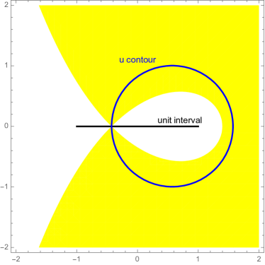
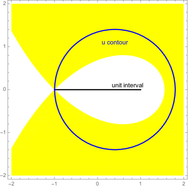
Here, the u๐‘ขu contour is a positively oriented (i.e., counterclockwise) simple loop around [โˆ’1,1]11[-1,1].

Refer to caption
Refer to caption
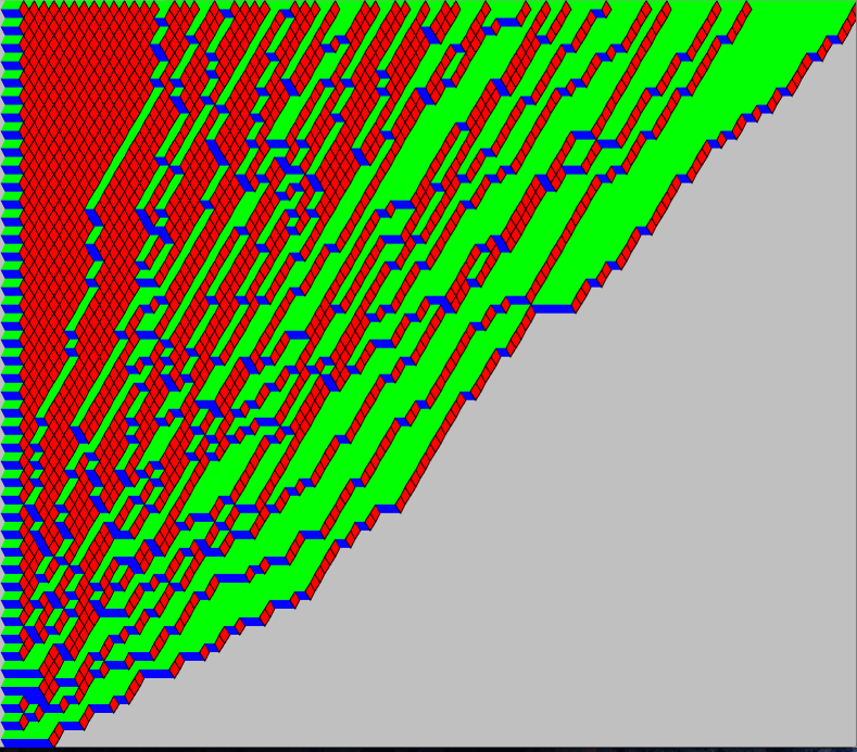
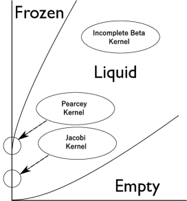
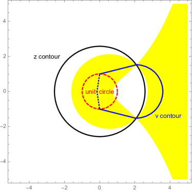
Figure 5: The hydrodynamic limit capturing average behavior indicates a densely-packed region of inactivity (โ€œfrozenโ€) and a central region of activity (โ€œliquidโ€), with the remaining area unreached (โ€œemptyโ€). Notably, the orthogonal and symplectic cases feature the same curves delineating these regions, which are given analytically by Proposition 6.2; compare with Figure 4 of [14].

Although the correlation kernel (7) of Theorem 1.2 may appear unwieldy at first, its double integral expression allows for asymptotic expansions leading to refined limiting results. Define the region ๐’Ÿlโ€‹iโ€‹qโ€‹uโ€‹iโ€‹dsuperscript๐’Ÿ๐‘™๐‘–๐‘ž๐‘ข๐‘–๐‘‘\mathcal{D}^{liquid} of nontrivial hydrodynamic limiting behavior as the collection of locations and times with a positive chance of either seeing a particle or not:

๐’Ÿlโ€‹iโ€‹qโ€‹uโ€‹iโ€‹d:={(ฯ„,ฮฝ,ฮท)โˆˆโ„+ร—โ„+ร—โ„+:0<limNโ†’โˆžฯ~1[Nโ€‹ฯ„]โ€‹(([Nโ€‹ฮฝ],[Nโ€‹ฮท]))<1}.assignsuperscript๐’Ÿ๐‘™๐‘–๐‘ž๐‘ข๐‘–๐‘‘conditional-set๐œ๐œˆ๐œ‚subscriptโ„subscriptโ„subscriptโ„0subscriptโ†’๐‘subscriptsuperscript~๐œŒdelimited-[]๐‘๐œ1delimited-[]๐‘๐œˆdelimited-[]๐‘๐œ‚1\mathcal{D}^{liquid}:=\left\{(\tau,\nu,\eta)\in\mathbb{R}_{+}\times\mathbb{R}_{+}\times\mathbb{R}_{+}:0<\lim_{N\to\infty}\widetilde{\rho}^{[N\tau]}_{1}(([N\nu],[N\eta]))<1\right\}. (8)

Under this hydrodynamic scaling, the method of steepest descent applied directly to the kernel (7) shows that ๐’Ÿlโ€‹iโ€‹qโ€‹uโ€‹iโ€‹dsuperscript๐’Ÿ๐‘™๐‘–๐‘ž๐‘ข๐‘–๐‘‘\mathcal{D}^{liquid} is exactly the region of (ฯ„,ฮฝ,ฮท)โˆˆโ„+3๐œ๐œˆ๐œ‚superscriptsubscriptโ„3(\tau,\nu,\eta)\in\mathbb{R}_{+}^{3} where the function

Sโ€‹(z)=Sฯ„,ฮฝ,ฮทโ€‹(z):=ฯ„โ€‹z+zโˆ’12โˆ’ฮฝโ€‹logโกz+ฮทโ€‹logโก(z+zโˆ’12โˆ’1).๐‘†๐‘งsubscript๐‘†๐œ๐œˆ๐œ‚๐‘งassign๐œ๐‘งsuperscript๐‘ง12๐œˆ๐‘ง๐œ‚๐‘งsuperscript๐‘ง121S(z)=S_{\tau,\nu,\eta}(z):=\tau\frac{z+z^{-1}}{2}-\nu\log z+\eta\log\left(\frac{z+z^{-1}}{2}-1\right). (9)

has a unique critical point z0=z0โ€‹(ฯ„,ฮฝ,ฮท)subscript๐‘ง0subscript๐‘ง0๐œ๐œˆ๐œ‚z_{0}=z_{0}(\tau,\nu,\eta) in โ„โˆ–๐”ปโ„๐”ป\mathbb{H}\setminus\mathbb{D}. Similarly define ๐’Ÿfโ€‹rโ€‹oโ€‹zโ€‹eโ€‹nsuperscript๐’Ÿ๐‘“๐‘Ÿ๐‘œ๐‘ง๐‘’๐‘›\mathcal{D}^{frozen} to be the region where we are sure to find particles in this limit, and ๐’Ÿeโ€‹mโ€‹pโ€‹tโ€‹ysuperscript๐’Ÿ๐‘’๐‘š๐‘๐‘ก๐‘ฆ\mathcal{D}^{empty} where there can be none; more precisely, these are the regions where the limit in (8) is 111 and 00, respectively. See Figure 5 for a depiction of these regions. To identify the nontrivial limit in the liquid region, define the incomplete beta kernel by

Bโ€‹(k;l|ฮถ):=12โ€‹ฯ€โ€‹iโ€‹โˆฎฮถยฏฮถ(1โˆ’z)kโ€‹zโˆ’(l+1)โ€‹๐‘‘z,assign๐ต๐‘˜conditional๐‘™๐œ12๐œ‹๐‘–superscriptsubscriptcontour-integralยฏ๐œ๐œsuperscript1๐‘ง๐‘˜superscript๐‘ง๐‘™1differential-d๐‘งB(k;l|\zeta):=\frac{1}{2\pi i}\oint_{\overline{\zeta}}^{\zeta}(1-z)^{k}z^{-(l+1)}dz,

where the contour crosses (0,1)01(0,1) if kโ‰ฅ0๐‘˜0k\geq 0 and (โˆ’โˆž,0)0(-\infty,0) if k<0๐‘˜0k<0. This kernel serves as a generalization of the sine kernel to describe bulk limits of the Schur process in [40] by Okounkovโ€“Reshetikhin.

Theorem 1.3.

(Bulk Limit: Incomplete Beta Kernel) Let (ฯ„,ฮฝ,ฮท)โˆˆ๐’Ÿlโ€‹iโ€‹qโ€‹uโ€‹iโ€‹d๐œ๐œˆ๐œ‚superscript๐’Ÿ๐‘™๐‘–๐‘ž๐‘ข๐‘–๐‘‘(\tau,\nu,\eta)\in\mathcal{D}^{liquid} and let z0=z0โ€‹(ฯ„,ฮฝ,ฮท)subscript๐‘ง0subscript๐‘ง0๐œ๐œˆ๐œ‚z_{0}=z_{0}(\tau,\nu,\eta) be the unique critical point of (9) in โ„โˆ–๐”ปโ„๐”ป\mathbb{H}\setminus\mathbb{D}. Assume ฮณโ‰ฅ0๐›พ0\gamma\geq 0, (si,ni)โˆˆโ„คโ‰ฅ0ร—โ„ค>0subscript๐‘ ๐‘–subscript๐‘›๐‘–subscriptโ„คabsent0subscriptโ„คabsent0(s_{i},n_{i})\in\mathbb{Z}_{\geq 0}\times\mathbb{Z}_{>0}, 1โ‰คiโ‰คk1๐‘–๐‘˜1\leq i\leq k, depend on N๐‘N in such a way that ฮณโˆผNโ€‹ฯ„>0similar-to๐›พ๐‘๐œ0\gamma\sim N\tau>0, siโˆผNโ€‹ฮฝ>0similar-tosubscript๐‘ ๐‘–๐‘๐œˆ0s_{i}\sim N\nu>0, and rniโˆผNโ€‹ฮท>0similar-tosubscript๐‘Ÿsubscript๐‘›๐‘–๐‘๐œ‚0r_{n_{i}}\sim N\eta>0. Assume the differences siโˆ’sjsubscript๐‘ ๐‘–subscript๐‘ ๐‘—s_{i}-s_{j}, niโˆ’njsubscript๐‘›๐‘–subscript๐‘›๐‘—n_{i}-n_{j} are of constant order. Then as Nโ†’โˆžโ†’๐‘N\to\infty,

ฯ~kฮณโ€‹((s1,n1),โ€ฆ,(sk,nk))โ†’det[Bโ€‹(niโˆ’nj;(siโˆ’sj)+(niโˆ’nj)โˆ’(rniโˆ’rnj)|z0)]i,j=1k.โ†’subscriptsuperscript~๐œŒ๐›พ๐‘˜subscript๐‘ 1subscript๐‘›1โ€ฆsubscript๐‘ ๐‘˜subscript๐‘›๐‘˜superscriptsubscriptdelimited-[]๐ตsubscript๐‘›๐‘–subscript๐‘›๐‘—subscript๐‘ ๐‘–subscript๐‘ ๐‘—subscript๐‘›๐‘–subscript๐‘›๐‘—conditionalsubscript๐‘Ÿsubscript๐‘›๐‘–subscript๐‘Ÿsubscript๐‘›๐‘—subscript๐‘ง0๐‘–๐‘—1๐‘˜\widetilde{\rho}^{\gamma}_{k}((s_{1},n_{1}),\ldots,(s_{k},n_{k}))\to\det[B(n_{i}-n_{j};(s_{i}-s_{j})+(n_{i}-n_{j})-(r_{n_{i}}-r_{n_{j}})|z_{0})]_{i,j=1}^{k}.

At the edges of the liquid region ๐’Ÿlโ€‹iโ€‹qโ€‹uโ€‹iโ€‹dsuperscript๐’Ÿ๐‘™๐‘–๐‘ž๐‘ข๐‘–๐‘‘\mathcal{D}^{liquid}, we find variants of the Jacobi and Pearcey kernels of Borodinโ€“Kuan [13, 14]. The first of these types arises in the large time limit at a finite distance from the wall, away from the corner of the phase transition; it only seems to have appeared so far in the similar contexts of [14] and [34], though with different Jacobi polynomials.

Theorem 1.4.

(Edge Limit: Discrete Jacobi Kernel) Assume ฮณโ‰ฅ0๐›พ0\gamma\geq 0, (si,ni)โˆˆโ„คโ‰ฅ0ร—โ„ค>0subscript๐‘ ๐‘–subscript๐‘›๐‘–subscriptโ„คabsent0subscriptโ„คabsent0(s_{i},n_{i})\in\mathbb{Z}_{\geq 0}\times\mathbb{Z}_{>0}, 1โ‰คiโ‰คk1๐‘–๐‘˜1\leq i\leq k, depend on N๐‘N in such a way that ฮณโˆผNโ€‹ฯ„>0similar-to๐›พ๐‘๐œ0\gamma\sim N\tau>0, rniโˆผNโ€‹ฮท>0similar-tosubscript๐‘Ÿsubscript๐‘›๐‘–๐‘๐œ‚0r_{n_{i}}\sim N\eta>0 but the sisubscript๐‘ ๐‘–s_{i} are fixed and finite. Assume only the differences niโˆ’njsubscript๐‘›๐‘–subscript๐‘›๐‘—n_{i}-n_{j} are of constant order. Then as Nโ†’โˆžโ†’๐‘N\to\infty,

ฯ~kฮณโ€‹((s1,n1),โ€ฆ,(sk,nk))โ†’{det[Lโ€‹((si,ni),(sj,nj)|1โˆ’ฮท/ฯ„)]i,j=1k,ifโ€‹ 1โˆ’ฮท/ฯ„>โˆ’11,ifโ€‹ 1โˆ’ฮท/ฯ„โ‰คโˆ’1โ†’subscriptsuperscript~๐œŒ๐›พ๐‘˜subscript๐‘ 1subscript๐‘›1โ€ฆsubscript๐‘ ๐‘˜subscript๐‘›๐‘˜casessuperscriptsubscriptdelimited-[]๐ฟsubscript๐‘ ๐‘–subscript๐‘›๐‘–conditionalsubscript๐‘ ๐‘—subscript๐‘›๐‘—1๐œ‚๐œ๐‘–๐‘—1๐‘˜if1๐œ‚๐œ11if1๐œ‚๐œ1\widetilde{\rho}^{\gamma}_{k}((s_{1},n_{1}),\ldots,(s_{k},n_{k}))\to\begin{cases}\det[L((s_{i},n_{i}),(s_{j},n_{j})|1-\eta/\tau)]_{i,j=1}^{k},&\text{if}\ \ 1-\eta/\tau>-1\\ 1,&\text{if}\ \ 1-\eta/\tau\leq-1\end{cases}

where the discrete Jacobi kernel L๐ฟL is given explicitly, for (s,n),(t,m)โˆˆโ„คโ‰ฅ0ร—โ„ค>0๐‘ ๐‘›๐‘ก๐‘šsubscriptโ„คabsent0subscriptโ„คabsent0(s,n),(t,m)\in\mathbb{Z}_{\geq 0}\times\mathbb{Z}_{>0}, by

Lโ€‹((s,n),(t,m)|ฯต):=2ฮฑn+1/2ฯ€โ€‹โˆซโˆ’11[1(nโ‰ฅm)+1[โˆ’1,ฯต]โ€‹(x)]โ€‹Js,ฮฑnโ€‹(x)โ€‹Jt,ฮฑmโ€‹(x)โ€‹(1โˆ’x)rnโˆ’rm+ฮฑnโ€‹(1+x)1/2โ€‹๐‘‘x.assign๐ฟ๐‘ ๐‘›conditional๐‘ก๐‘šitalic-ฯตabsentsuperscript2subscript๐›ผ๐‘›12๐œ‹superscriptsubscript11delimited-[]subscript1๐‘›๐‘šsubscript11italic-ฯต๐‘ฅsubscript๐ฝ๐‘ subscript๐›ผ๐‘›๐‘ฅsubscript๐ฝ๐‘กsubscript๐›ผ๐‘š๐‘ฅsuperscript1๐‘ฅsubscript๐‘Ÿ๐‘›subscript๐‘Ÿ๐‘šsubscript๐›ผ๐‘›superscript1๐‘ฅ12differential-d๐‘ฅ\begin{aligned} L((s,n),(t,m)|\epsilon):=&\frac{2^{\alpha_{n}+1/2}}{\pi}\int_{-1}^{1}[1_{(n\geq m)}+1_{[-1,\epsilon]}(x)]J_{s,\alpha_{n}}(x)J_{t,\alpha_{m}}(x)(1-x)^{r_{n}-r_{m}+\alpha_{n}}(1+x)^{1/2}dx\\ \end{aligned}. (10)

Our last result shows the corner of the phase transition (i.e., near where the regions ๐’Ÿfโ€‹rโ€‹oโ€‹zโ€‹eโ€‹nsuperscript๐’Ÿ๐‘“๐‘Ÿ๐‘œ๐‘ง๐‘’๐‘›\mathcal{D}^{frozen} and ๐’Ÿlโ€‹iโ€‹qโ€‹uโ€‹iโ€‹dsuperscript๐’Ÿ๐‘™๐‘–๐‘ž๐‘ข๐‘–๐‘‘\mathcal{D}^{liquid} meet the wall) exhibits a 1/4141/4-exponent in its fluctuation scale, providing additional rigorous evidence of the universality of this growth exponent in the class of anisotropic KPZ with a wall. The evolving stepped-surface interpretation indicated by Figure 1 allows one to define a height function as โ€œthe number of particles at that point and to the rightโ€. The fluctuations about its mean should be described (at least formally) by the anisotropic KPZ equation, a stochastic heat equation of the form

โˆ‚th=ฮฝxโ€‹โˆ‚x2h+ฮฝyโ€‹โˆ‚y2h+12โ€‹ฮปxโ€‹(โˆ‚xh)2+12โ€‹ฮปyโ€‹(โˆ‚yh)2+ฮพ,subscript๐‘กโ„Žsubscript๐œˆ๐‘ฅsuperscriptsubscript๐‘ฅ2โ„Žsubscript๐œˆ๐‘ฆsuperscriptsubscript๐‘ฆ2โ„Ž12subscript๐œ†๐‘ฅsuperscriptsubscript๐‘ฅโ„Ž212subscript๐œ†๐‘ฆsuperscriptsubscript๐‘ฆโ„Ž2๐œ‰\partial_{t}h=\nu_{x}\partial_{x}^{2}h+\nu_{y}\partial_{y}^{2}h+\frac{1}{2}\lambda_{x}(\partial_{x}h)^{2}+\frac{1}{2}\lambda_{y}(\partial_{y}h)^{2}+\xi,

where ฮพ๐œ‰\xi is a spaceโ€“time white noise and ฮปx,ฮปysubscript๐œ†๐‘ฅsubscript๐œ†๐‘ฆ\lambda_{x},\lambda_{y} have different signs (should they have the same sign, this equation reduces to the classical KPZ equation). We do not explore this equation in this work, we only note its relevance for future research; see, e.g., Borodinโ€“Ferrari [10] for more discussion. Such rigorous results for systems with a wall still seem to be rare; the author only knows of [5, 14, 34, 36]. The kernel arising in our setting at this critical corner point appears to be an instance of a general family of Pearcey-type posited in Remark 1.5 of [36].

Theorem 1.5.

(Edge Limit: Pearcey Kernel) Let ฯ~ฮ”ฮณ,ksubscriptsuperscript~๐œŒ๐›พ๐‘˜ฮ”\widetilde{\rho}^{\gamma,k}_{\Delta} denote the k๐‘˜kth correlation function of the determinantal process determined by the complementary process (๐’ณ~โ€‹(ฮณ))csuperscript~๐’ณ๐›พ๐‘(\widetilde{\mathcal{X}}(\gamma))^{c}. Assume ฮณโ‰ฅ0๐›พ0\gamma\geq 0, (si,ni)โˆˆโ„คโ‰ฅ0ร—โ„ค>0subscript๐‘ ๐‘–subscript๐‘›๐‘–subscriptโ„คabsent0subscriptโ„คabsent0(s_{i},n_{i})\in\mathbb{Z}_{\geq 0}\times\mathbb{Z}_{>0}, 1โ‰คiโ‰คk1๐‘–๐‘˜1\leq i\leq k, depend on N๐‘N in such a way that ฮณโˆผN/2similar-to๐›พ๐‘2\gamma\sim N/2, siโˆผN1/4โ€‹ฮฝi>0similar-tosubscript๐‘ ๐‘–superscript๐‘14subscript๐œˆ๐‘–0s_{i}\sim N^{1/4}\nu_{i}>0, and rniโˆ’NโˆผNโ€‹ฮทi>0similar-tosubscript๐‘Ÿsubscript๐‘›๐‘–๐‘๐‘subscript๐œ‚๐‘–0r_{n_{i}}-N\sim\sqrt{N}\eta_{i}>0. Then as Nโ†’โˆžโ†’๐‘N\to\infty,

Nk/4โ‹…ฯ~ฮ”ฮณ,kโ‹…superscript๐‘๐‘˜4subscriptsuperscript~๐œŒ๐›พ๐‘˜ฮ”\displaystyle N^{k/4}\cdot\widetilde{\rho}^{\gamma,k}_{\Delta} ((s1,n1),โ€ฆ,(sk,nk))โ†’det[๐’ฆโ€‹((ฮฝi,ฮทi),(ฮฝj,ฮทj))]i,j=1k,โ†’subscript๐‘ 1subscript๐‘›1โ€ฆsubscript๐‘ ๐‘˜subscript๐‘›๐‘˜superscriptsubscriptdelimited-[]๐’ฆsubscript๐œˆ๐‘–subscript๐œ‚๐‘–subscript๐œˆ๐‘—subscript๐œ‚๐‘—๐‘–๐‘—1๐‘˜\displaystyle((s_{1},n_{1}),\ldots,(s_{k},n_{k}))\to\det[\mathcal{K}((\nu_{i},\eta_{i}),(\nu_{j},\eta_{j}))]_{i,j=1}^{k},

where the Pearcey Kernel ๐’ฆ๐’ฆ\mathcal{K} is given explicitly by

๐’ฆโ€‹((ฮฝ1,ฮท1),(ฮฝ2,ฮท2)):=assign๐’ฆsubscript๐œˆ1subscript๐œ‚1subscript๐œˆ2subscript๐œ‚2absent\displaystyle\mathcal{K}((\nu_{1},\eta_{1}),(\nu_{2},\eta_{2})):= 1(ฮท1>ฮท2)โ€‹1ฯ€โ€‹(ฮท1โˆ’ฮท2)โ€‹(expโก[โˆ’(ฮฝ1+ฮฝ2)2ฮท1โˆ’ฮท2]โˆ’expโก[โˆ’(ฮฝ1โˆ’ฮฝ2)2ฮท1โˆ’ฮท2])subscript1subscript๐œ‚1subscript๐œ‚21๐œ‹subscript๐œ‚1subscript๐œ‚2superscriptsubscript๐œˆ1subscript๐œˆ22subscript๐œ‚1subscript๐œ‚2superscriptsubscript๐œˆ1subscript๐œˆ22subscript๐œ‚1subscript๐œ‚2\displaystyle 1_{(\eta_{1}>\eta_{2})}\frac{1}{\sqrt{\pi(\eta_{1}-\eta_{2})}}\left(\exp\left[-\frac{(\nu_{1}+\nu_{2})^{2}}{\eta_{1}-\eta_{2}}\right]-\exp\left[-\frac{(\nu_{1}-\nu_{2})^{2}}{\eta_{1}-\eta_{2}}\right]\right)
+2ฯ€โ€‹12โ€‹ฯ€โ€‹iโ€‹โˆซโˆ’iโ€‹โˆžiโ€‹โˆžโˆซ0โˆže(uโ€ฒ)2โˆ’(xโ€ฒ)28+ฮท2โ€‹uโ€ฒโˆ’ฮท1โ€‹xโ€ฒ2โ€‹sinโก[ฮฝ1โ€‹2โ€‹xโ€ฒ]โ€‹sinโก[ฮฝ2โ€‹2โ€‹uโ€ฒ]โ€‹dโ€‹xโ€ฒโ€‹dโ€‹uโ€ฒuโ€ฒโ€‹(uโ€ฒโˆ’xโ€ฒ).2๐œ‹12๐œ‹๐‘–superscriptsubscript๐‘–๐‘–superscriptsubscript0superscript๐‘’superscriptsuperscript๐‘ขโ€ฒ2superscriptsuperscript๐‘ฅโ€ฒ28subscript๐œ‚2superscript๐‘ขโ€ฒsubscript๐œ‚1superscript๐‘ฅโ€ฒ2subscript๐œˆ12superscript๐‘ฅโ€ฒsubscript๐œˆ22superscript๐‘ขโ€ฒ๐‘‘superscript๐‘ฅโ€ฒ๐‘‘superscript๐‘ขโ€ฒsuperscript๐‘ขโ€ฒsuperscript๐‘ขโ€ฒsuperscript๐‘ฅโ€ฒ\displaystyle+\frac{\sqrt{2}}{\pi}\frac{1}{2\pi i}\int_{-i\infty}^{i\infty}\int_{0}^{\infty}e^{\frac{(u^{\prime})^{2}-(x^{\prime})^{2}}{8}+\frac{\eta_{2}u^{\prime}-\eta_{1}x^{\prime}}{2}}\sin[\nu_{1}\sqrt{2x^{\prime}}]\sin[\nu_{2}\sqrt{2u^{\prime}}]\frac{dx^{\prime}du^{\prime}}{\sqrt{u^{\prime}}(u^{\prime}-x^{\prime})}.
Acknowledgements.

The author would like to thank Renรฉ Carmona, Allen Knutson, Daniel Lacker, Ramon Van Handel, and Mykhaylo Shkolnikov for many helpful discussions, as well as Jon Warren for an informative private correspondence. I would especially like to thank Jeffrey Kuan, for early encouragement and consistently valuable guidance, as well as for supporting a simulation of the symplectic growth process at http://www.math.harvard.edu/~jkuan/Cerenzia.html.

Part of this research was performed while the author was visiting the Institute for Pure and Applied Mathematics (IPAM), which is supported by the National Science Foundation; the author was also partially supported by NSF: DMS-0806591.

2 Diffusive scaling limit and repulsion of Dyson gaps

2.1 Time-dependent Skorokhod problem and Skorokhod reflection map

The machinery of the extended Skorokhod map provides a remarkably natural and careful construction of our particle system and its diffusion limit. A solution to the Skorokhod problem (SP) of reflecting a particle ฯˆ๐œ“\psi in a (potentially time-dependent) interval [โ„“,r]โ„“๐‘Ÿ[\ell,r], โ„“โ‰คrโ„“๐‘Ÿ\ell\leq r, is a pair (ฯ•,ฮท)italic-ฯ•๐œ‚(\phi,\eta) where ฮท๐œ‚\eta โ€œpushesโ€ the particle ฯˆ๐œ“\psi to remain in [โ„“,r]โ„“๐‘Ÿ[\ell,r] and the resulting reflected movements ฯ•=ฯˆ+ฮทโˆˆ[โ„“,r]italic-ฯ•๐œ“๐œ‚โ„“๐‘Ÿ\phi=\psi+\eta\in[\ell,r] should be regular; classically, ฮท๐œ‚\eta should be of bounded variation and (ฯ•,ฮท)italic-ฯ•๐œ‚(\phi,\eta) should satisfy the familiar conditions

โˆซ0โˆž1(โ„“โ€‹(s)<ฯ•โ€‹(s))โ€‹๐‘‘ฮทโ„“โ€‹(s)=โˆซ0โˆž1(ฯ•โ€‹(s)<rโ€‹(s))โ€‹๐‘‘ฮทrโ€‹(s)=0,superscriptsubscript0subscript1โ„“๐‘ italic-ฯ•๐‘ differential-dsubscript๐œ‚โ„“๐‘ superscriptsubscript0subscript1italic-ฯ•๐‘ ๐‘Ÿ๐‘ differential-dsubscript๐œ‚๐‘Ÿ๐‘ 0\int_{0}^{\infty}1_{(\ell(s)<\phi(s))}d\eta_{\ell}(s)=\int_{0}^{\infty}1_{(\phi(s)<r(s))}d\eta_{r}(s)=0, (11)

where ฮทโ„“,ฮทrsubscript๐œ‚โ„“subscript๐œ‚๐‘Ÿ\eta_{\ell},\eta_{r} are nondecreasing functions affording the (minimal) decomposition ฮท=ฮทโ„“โˆ’ฮทr๐œ‚subscript๐œ‚โ„“subscript๐œ‚๐‘Ÿ\eta=\eta_{\ell}-\eta_{r}. But as explained in Section 1.2.1, the conditions (11) are too restrictive for our situation. To state a weaker notion of solution, let Dโ€‹(โ„+,S)๐ทsubscriptโ„๐‘†D(\mathbb{R}_{+},S) be the space of right-continuous functions with left limits on โ„+subscriptโ„\mathbb{R}_{+} that take values in a separable complete metric space S๐‘†S. Write D:=Dโ€‹(โ„+,โ„)assign๐ท๐ทsubscriptโ„โ„D:=D(\mathbb{R}_{+},\mathbb{R}), Dโˆ’:=Dโ€‹(โ„+,[โˆ’โˆž,โˆž))assignsuperscript๐ท๐ทsubscriptโ„D^{-}:=D(\mathbb{R}_{+},[-\infty,\infty)), and D+:=Dโ€‹(โ„+,(โˆ’โˆž,โˆž])assignsuperscript๐ท๐ทsubscriptโ„D^{+}:=D(\mathbb{R}_{+},(-\infty,\infty]).

Definition 2.1.

(Definition 2.2, [20]) Given (โ„“,r,ฯˆ)โˆˆDโˆ’ร—D+ร—Dโ„“๐‘Ÿ๐œ“superscript๐ทsuperscript๐ท๐ท(\ell,r,\psi)\in D^{-}\times D^{+}\times D with โ„“โ‰คrโ„“๐‘Ÿ\ell\leq r, a pair (ฯ•,ฮท)โˆˆDร—Ditalic-ฯ•๐œ‚๐ท๐ท(\phi,\eta)\in D\times D solves the extended Skorokhod problem (ESP) on [โ„“,r]โ„“๐‘Ÿ[\ell,r] for ฯˆ๐œ“\psi if

  1. 1.

    ฯ•โ€‹(t)=ฯˆโ€‹(t)+ฮทโ€‹(t)โˆˆ[โ„“โ€‹(t),rโ€‹(t)]italic-ฯ•๐‘ก๐œ“๐‘ก๐œ‚๐‘กโ„“๐‘ก๐‘Ÿ๐‘ก\phi(t)=\psi(t)+\eta(t)\in[\ell(t),r(t)] for tโ‰ฅ0๐‘ก0t\geq 0

  2. 2.

    For 0โ‰คs<t<โˆž0๐‘ ๐‘ก0\leq s<t<\infty,

    ฮทโ€‹(t)โˆ’ฮทโ€‹(s)โ‰ฅ0๐œ‚๐‘ก๐œ‚๐‘ 0\eta(t)-\eta(s)\geq 0, if ฯ•<ritalic-ฯ•๐‘Ÿ\phi<r on (s,t]๐‘ ๐‘ก(s,t]; and ฮทโ€‹(s)โˆ’ฮทโ€‹(sโˆ’)โ‰ฅ0๐œ‚๐‘ ๐œ‚limit-from๐‘ 0\eta(s)-\eta(s-)\geq 0, if ฯ•โ€‹(s)<rโ€‹(s)italic-ฯ•๐‘ ๐‘Ÿ๐‘ \phi(s)<r(s)

    ฮทโ€‹(t)โˆ’ฮทโ€‹(s)โ‰ค0๐œ‚๐‘ก๐œ‚๐‘ 0\eta(t)-\eta(s)\leq 0, if โ„“<ฯ•โ„“italic-ฯ•\ell<\phi on (s,t]๐‘ ๐‘ก(s,t]; and ฮทโ€‹(s)โˆ’ฮทโ€‹(sโˆ’)โ‰ค0๐œ‚๐‘ ๐œ‚limit-from๐‘ 0\eta(s)-\eta(s-)\leq 0, if โ„“โ€‹(s)<ฯ•โ€‹(s)โ„“๐‘ italic-ฯ•๐‘ \ell(s)<\phi(s)

Given (โ„“,r,ฯˆ)โˆˆDโˆ’ร—D+ร—Dโ„“๐‘Ÿ๐œ“superscript๐ทsuperscript๐ท๐ท(\ell,r,\psi)\in D^{-}\times D^{+}\times D with โ„“โ‰คrโ„“๐‘Ÿ\ell\leq r, an explicit candidate for the reflected process ฯ•italic-ฯ•\phi is provided by the extended Skorokhod map ฮ“ยฏโ€‹(โ„“,r|ฯˆ):=ฯˆโˆ’ฮžโ„“,rโ€‹(ฯˆ)assignยฏฮ“โ„“conditional๐‘Ÿ๐œ“๐œ“subscriptฮžโ„“๐‘Ÿ๐œ“\overline{\Gamma}(\ell,r|\psi):=\psi-\Xi_{\ell,r}(\psi), where

ฮžโ„“,rsubscriptฮžโ„“๐‘Ÿ\displaystyle\Xi_{\ell,r} (ฯˆ)โ€‹(t):=maxโก((ฯˆโ€‹(0)โˆ’rโ€‹(0))+โˆงinfuโˆˆ[0,t](ฯˆโ€‹(u)โˆ’โ„“โ€‹(u)),supsโˆˆ[0,t][(ฯˆโ€‹(s)โˆ’rโ€‹(s))โˆงinfuโˆˆ[s,t](ฯˆโ€‹(u)โˆ’โ„“โ€‹(u))]).assign๐œ“๐‘กsuperscript๐œ“0๐‘Ÿ0subscriptinfimum๐‘ข0๐‘ก๐œ“๐‘ขโ„“๐‘ขsubscriptsupremum๐‘ 0๐‘กdelimited-[]๐œ“๐‘ ๐‘Ÿ๐‘ subscriptinfimum๐‘ข๐‘ ๐‘ก๐œ“๐‘ขโ„“๐‘ข\displaystyle(\psi)(t):=\max\bigg{(}(\psi(0)-r(0))^{+}\wedge\inf_{u\in[0,t]}(\psi(u)-\ell(u)),\sup_{s\in[0,t]}[(\psi(s)-r(s))\wedge\inf_{u\in[s,t]}(\psi(u)-\ell(u))]\bigg{)}.

Note some simplifications: if rโ‰กโˆž๐‘Ÿr\equiv\infty, then ฮžโ„“,โˆžโ€‹(ฯˆ)โ€‹(t)=โˆ’supsโˆˆ[0,t][โ„“โ€‹(s)โˆ’ฯˆโ€‹(s)]+subscriptฮžโ„“๐œ“๐‘กsubscriptsupremum๐‘ 0๐‘กsuperscriptdelimited-[]โ„“๐‘ ๐œ“๐‘ \Xi_{\ell,\infty}(\psi)(t)=-\sup_{s\in[0,t]}[\ell(s)-\psi(s)]^{+}, tโ‰ฅ0๐‘ก0t\geq 0; also, at the initial time 00,

ฮžโ„“,rโ€‹(ฯˆ)โ€‹(0)=[ฯˆโ€‹(0)โˆ’rโ€‹(0)]+โˆง[ฯˆโ€‹(0)โˆ’โ„“โ€‹(0)]โˆ’.subscriptฮžโ„“๐‘Ÿ๐œ“0superscriptdelimited-[]๐œ“0๐‘Ÿ0superscriptdelimited-[]๐œ“0โ„“0\Xi_{\ell,r}(\psi)(0)=[\psi(0)-r(0)]^{+}\wedge[\psi(0)-\ell(0)]^{-}. (12)

In words then, ฮ“ยฏโ€‹(โ„“,r|ฯˆ)ยฏฮ“โ„“conditional๐‘Ÿ๐œ“\overline{\Gamma}(\ell,r|\psi) starts by putting the particle ฯˆ๐œ“\psi at the nearest point in [โ„“,r]โ„“๐‘Ÿ[\ell,r] and maintains its increments except for putting those that land outside of [โ„“,r]โ„“๐‘Ÿ[\ell,r] again at the nearest point inside. Theorem 2.6 and Proposition 2.8 of [20] show ฮ“ยฏยฏฮ“\overline{\Gamma} is a jointly continuous function on Dโˆ’ร—D+ร—Dsuperscript๐ทsuperscript๐ท๐ทD^{-}\times D^{+}\times D (each topologized by uniform convergence on compacts) and provides the unique solution

(ฯ•,ฮท):=(ฮ“ยฏโ€‹(โ„“,r|ฯˆ),ฮ“ยฏโ€‹(โ„“,r|ฯˆ)โˆ’ฯˆ)assignitalic-ฯ•๐œ‚ยฏฮ“โ„“conditional๐‘Ÿ๐œ“ยฏฮ“โ„“conditional๐‘Ÿ๐œ“๐œ“(\phi,\eta):=(\overline{\Gamma}(\ell,r|\psi),\overline{\Gamma}(\ell,r|\psi)-\psi)

to the associated ESP on [โ„“,r]โ„“๐‘Ÿ[\ell,r] for ฯˆ๐œ“\psi. The condition inftโˆˆ[t1,t2](rโ€‹(t)โˆ’โ„“โ€‹(t))>0subscriptinfimum๐‘กsubscript๐‘ก1subscript๐‘ก2๐‘Ÿ๐‘กโ„“๐‘ก0\inf_{t\in[t_{1},t_{2}]}(r(t)-\ell(t))>0, 0โ‰คt1<t20subscript๐‘ก1subscript๐‘ก20\leq t_{1}<t_{2}, is sufficient for (ฯ•,ฮท)italic-ฯ•๐œ‚(\phi,\eta) to satisfy the more regular conditions (11) on [t1,t2]subscript๐‘ก1subscript๐‘ก2[t_{1},t_{2}]; cf. Corollary 2.4 of [20].

2.2 First construction of symplectic Plancherel growth and continuum universal limit

Fix nโ‰ฅ1๐‘›1n\geq 1. Consider the collection Xโ€‹(t):={Xikโ€‹(t)|1โ‰คkโ‰คn, 1โ‰คiโ‰คrk}assign๐‘‹๐‘กconditional-setsubscriptsuperscript๐‘‹๐‘˜๐‘–๐‘กformulae-sequence1๐‘˜๐‘›1๐‘–subscript๐‘Ÿ๐‘˜X(t):=\{X^{k}_{i}(t)|1\leq k\leq n,\ 1\leq i\leq r_{k}\}, tโ‰ฅ0๐‘ก0t\geq 0, of continuous time simple random walks Xiksubscriptsuperscript๐‘‹๐‘˜๐‘–X^{k}_{i} started at 00, with jumps dictated by independent unit rate poisson processes. For a parameter N>0๐‘0N>0, consider the diffusively scaled versions Xยฏโ€‹(t;N):=Xtโ€‹N/Nassignยฏ๐‘‹๐‘ก๐‘subscript๐‘‹๐‘ก๐‘๐‘\bar{X}(t;N):=X_{tN}/\sqrt{N}. Construct a process (๐’ณโ€‹(t,N))tโ‰ฅ0subscript๐’ณ๐‘ก๐‘๐‘ก0(\mathcal{X}(t,N))_{t\geq 0} with components ๐’ณikโ€‹(t,N)subscriptsuperscript๐’ณ๐‘˜๐‘–๐‘ก๐‘\mathcal{X}^{k}_{i}(t,N) driven by Xยฏยฏ๐‘‹\bar{X} by setting ๐’ณ11:=ฮ“ยฏโ€‹(0,โˆž|Xยฏ11)assignsubscriptsuperscript๐’ณ11ยฏฮ“0conditionalsubscriptsuperscriptยฏ๐‘‹11\mathcal{X}^{1}_{1}:=\overline{\Gamma}(0,\infty|\bar{X}^{1}_{1}) and inductively for 2โ‰คkโ‰คn2๐‘˜๐‘›2\leq k\leq n,

๐’ณik:={ฮ“ยฏโ€‹(0,๐’ณiโˆ’1kโˆ’1โˆ’1/N|Xยฏik),ifi=rkwithkโ€‹oddฮ“ยฏโ€‹(๐’ณikโˆ’1+1/N,๐’ณiโˆ’1kโˆ’1โˆ’1/N|Xยฏik),otherwise forโ€‹ 1โ‰คiโ‰คrk,assignsubscriptsuperscript๐’ณ๐‘˜๐‘–casesยฏฮ“0subscriptsuperscript๐’ณ๐‘˜1๐‘–1conditional1๐‘subscriptsuperscriptยฏ๐‘‹๐‘˜๐‘–formulae-sequenceif๐‘–subscript๐‘Ÿ๐‘˜withkoddยฏฮ“subscriptsuperscript๐’ณ๐‘˜1๐‘–1๐‘subscriptsuperscript๐’ณ๐‘˜1๐‘–1conditional1๐‘subscriptsuperscriptยฏ๐‘‹๐‘˜๐‘–otherwise for1๐‘–subscript๐‘Ÿ๐‘˜\mathcal{X}^{k}_{i}:=\begin{cases}\overline{\Gamma}(0,\mathcal{X}^{k-1}_{i-1}-1/\sqrt{N}\big{|}\bar{X}^{k}_{i}),&\text{if}\ \ i=r_{k}\ \ \text{with}\ \ $k$\ \text{odd}\\ \overline{\Gamma}(\mathcal{X}^{k-1}_{i}+1/\sqrt{N},\mathcal{X}^{k-1}_{i-1}-1/\sqrt{N}\big{|}\bar{X}^{k}_{i}),&\text{otherwise for}\ 1\leq i\leq r_{k}\end{cases}, (13)

where our convention ๐’ณ0kโˆ’1โ‰กโˆžsubscriptsuperscript๐’ณ๐‘˜10\mathcal{X}^{k-1}_{0}\equiv\infty applies. This procedure determines deterministic maps ฮฆNSโ€‹Kโ€‹(Xยฏ)โ€‹(t)=๐’ณโ€‹(t,N)subscriptsuperscriptฮฆ๐‘†๐พ๐‘ยฏ๐‘‹๐‘ก๐’ณ๐‘ก๐‘\Phi^{SK}_{N}(\bar{X})(t)=\mathcal{X}(t,N).

Definition 2.2.

Symplectic Plancherel growth considered up to level nโ‰ฅ1๐‘›1n\geq 1 is characterized by the interlaced dynamics of the process ๐’ณโ€‹(ฮณ):=๐’ณโ€‹(ฮณ,1)assign๐’ณ๐›พ๐’ณ๐›พ1\mathcal{X}(\gamma):=\mathcal{X}(\gamma,1), ฮณโ‰ฅ0๐›พ0\gamma\geq 0, defined by (13).

Note 2.1.

By the simplification (12) at time t=0๐‘ก0t=0, ๐’ณโ€‹(0)๐’ณ0\mathcal{X}(0) is exactly the โ€œleftmostโ€ initial condition up to level n๐‘›n. However, Definition 2.2 refers to the interlaced dynamics and does not depend on this initial condition. In fact, the paper [27] illustrates how the results of this section hold for much more general dynamics and initial conditions, and a forthcoming technical report will show the dynamics of [14, 23, 24, 34, 48] all converge to the same system under diffusive scaling. It is only for continuity of focus and simplicity of presentation that we maintain our concrete setting.

The appropriate continuum state space for the diffusion limit is given by the collection ๐•n,pโ€‹aโ€‹tโ€‹hโ€‹scsubscriptsuperscript๐•๐‘๐‘›๐‘๐‘Ž๐‘กโ„Ž๐‘ \mathbb{J}^{c}_{n,paths} of arrays {yikโˆˆโ„+|1โ‰คkโ‰คn, 1โ‰คiโ‰คrk}conditional-setsubscriptsuperscript๐‘ฆ๐‘˜๐‘–subscriptโ„formulae-sequence1๐‘˜๐‘›1๐‘–subscript๐‘Ÿ๐‘˜\{y^{k}_{i}\in\mathbb{R}_{+}|1\leq k\leq n,\ 1\leq i\leq r_{k}\} of nonnegative real numbers satisfying

yk+1n+1โ‰คyknโ‰คykn+1, 1โ‰คkโ‰คrn.formulae-sequencesubscriptsuperscript๐‘ฆ๐‘›1๐‘˜1subscriptsuperscript๐‘ฆ๐‘›๐‘˜subscriptsuperscript๐‘ฆ๐‘›1๐‘˜1๐‘˜subscript๐‘Ÿ๐‘›y^{n+1}_{k+1}\leq y^{n}_{k}\leq y^{n+1}_{k},\ \ \ \ 1\leq k\leq r_{n}.

Consider the collection Bโ€‹(t):={Bikโ€‹(t)|1โ‰คkโ‰คn, 1โ‰คiโ‰คrk}assign๐ต๐‘กconditional-setsubscriptsuperscript๐ต๐‘˜๐‘–๐‘กformulae-sequence1๐‘˜๐‘›1๐‘–subscript๐‘Ÿ๐‘˜B(t):=\{B^{k}_{i}(t)|1\leq k\leq n,\ 1\leq i\leq r_{k}\}, tโ‰ฅ0๐‘ก0t\geq 0, of independent Brownian motions started at 00. Construct now a process (๐’ฒโ€‹(t))tโ‰ฅ0subscript๐’ฒ๐‘ก๐‘ก0(\mathcal{W}(t))_{t\geq 0} in ๐•n,pโ€‹aโ€‹tโ€‹hโ€‹scsubscriptsuperscript๐•๐‘๐‘›๐‘๐‘Ž๐‘กโ„Ž๐‘ \mathbb{J}^{c}_{n,paths} with components ๐’ฒiksubscriptsuperscript๐’ฒ๐‘˜๐‘–\mathcal{W}^{k}_{i} driven by (Bโ€‹(t))tโ‰ฅ0subscript๐ต๐‘ก๐‘ก0(B(t))_{t\geq 0} by setting ๐’ฒ11:=ฮ“ยฏโ€‹(0,โˆž|B11)assignsubscriptsuperscript๐’ฒ11ยฏฮ“0conditionalsubscriptsuperscript๐ต11\mathcal{W}^{1}_{1}:=\overline{\Gamma}(0,\infty|B^{1}_{1}) and inductively

๐’ฒik:=ฮ“ยฏโ€‹(๐’ฒikโˆ’1,๐’ฒiโˆ’1kโˆ’1|Bik),assignsubscriptsuperscript๐’ฒ๐‘˜๐‘–ยฏฮ“subscriptsuperscript๐’ฒ๐‘˜1๐‘–conditionalsubscriptsuperscript๐’ฒ๐‘˜1๐‘–1subscriptsuperscript๐ต๐‘˜๐‘–\mathcal{W}^{k}_{i}:=\overline{\Gamma}(\mathcal{W}^{k-1}_{i},\mathcal{W}^{k-1}_{i-1}|B^{k}_{i}), (14)

for 2โ‰คkโ‰คn2๐‘˜๐‘›2\leq k\leq n, 1โ‰คiโ‰คrk1๐‘–subscript๐‘Ÿ๐‘˜1\leq i\leq r_{k} (recall our notational convention). This procedure determines another deterministic map ฮจSโ€‹Kโ€‹(B):=๐’ฒassignsuperscriptฮจ๐‘†๐พ๐ต๐’ฒ\Psi^{SK}(B):=\mathcal{W}. Notice ฮฆNSโ€‹Kโ†’ฮจSโ€‹Kโ†’subscriptsuperscriptฮฆ๐‘†๐พ๐‘superscriptฮจ๐‘†๐พ\Phi^{SK}_{N}\to\Psi^{SK} as Nโ†’โˆžโ†’๐‘N\to\infty.

Proposition 2.3.

Fix nโ‰ฅ1๐‘›1n\geq 1 and write dn:=rnโ€‹(rn+1)/2+rnโˆ’1โ€‹(rnโˆ’1+1)/2assignsubscript๐‘‘๐‘›subscript๐‘Ÿ๐‘›subscript๐‘Ÿ๐‘›12subscript๐‘Ÿ๐‘›1subscript๐‘Ÿ๐‘›112d_{n}:=r_{n}(r_{n}+1)/2+r_{n-1}(r_{n-1}+1)/2. Then considered up to level n๐‘›n, the diffusively scaled symplectic Plancherel growth process (๐’ณโ€‹(t;N))tโ‰ฅ0subscript๐’ณ๐‘ก๐‘๐‘ก0(\mathcal{X}(t;N))_{t\geq 0} converges in law on Dโ€‹([0,โˆž),โ„dn)๐ท0superscriptโ„subscript๐‘‘๐‘›D([0,\infty),\mathbb{R}^{d_{n}}) to the interlaced reflecting system (๐’ฒโ€‹(t))tโ‰ฅ0subscript๐’ฒ๐‘ก๐‘ก0(\mathcal{W}(t))_{t\geq 0} of (14) with a wall started at ๐ŸŽโˆˆ๐•n,pโ€‹aโ€‹tโ€‹hโ€‹sc0subscriptsuperscript๐•๐‘๐‘›๐‘๐‘Ž๐‘กโ„Ž๐‘ \mathbf{0}\in\mathbb{J}^{c}_{n,paths}.

Proof.

For n=1๐‘›1n=1, the laws of Xยฏ11subscriptsuperscriptยฏ๐‘‹11\bar{X}^{1}_{1} converge on Dโ€‹([0,โˆž),โ„)๐ท0โ„D([0,\infty),\mathbb{R}) to the law of a standard Brownian motion (see, e.g., the much stronger Theorem 16.14 of [29], where convergence in the Skorokhod topology strengthens to convergence in the supremem norm topology since the limit is continuous). In turn, the law of the images ๐’ณโ€‹(t;N)=ฮ“ยฏโ€‹(0,โˆž|Xยฏ11โ€‹(โ‹…,N))โ€‹(t)๐’ณ๐‘ก๐‘ยฏฮ“0conditionalsubscriptsuperscriptยฏ๐‘‹11โ‹…๐‘๐‘ก\mathcal{X}(t;N)=\bar{\Gamma}(0,\infty|\bar{X}^{1}_{1}(\cdot,N))(t) converge to a standard reflected Brownian motion ฮ“ยฏโ€‹(0,โˆž|B11)โ€‹(t)=B11โ€‹(t)+supsโˆˆ[0,t][โˆ’B11โ€‹(s)]+ยฏฮ“0conditionalsubscriptsuperscript๐ต11๐‘กsubscriptsuperscript๐ต11๐‘กsubscriptsupremum๐‘ 0๐‘กsuperscriptdelimited-[]subscriptsuperscript๐ต11๐‘ \bar{\Gamma}(0,\infty|B^{1}_{1})(t)=B^{1}_{1}(t)+\sup_{s\in[0,t]}[-B^{1}_{1}(s)]^{+}.

For nโ‰ฅ2๐‘›2n\geq 2, assume that the statement of the theorem holds for all levels k๐‘˜k, 1โ‰คkโ‰คnโˆ’11๐‘˜๐‘›11\leq k\leq n-1, so that the restriction of ๐’ณโ€‹(t;N)๐’ณ๐‘ก๐‘\mathcal{X}(t;N) to these levels converges in law on Dโ€‹([0,โˆž),โ„dnโˆ’1)๐ท0superscriptโ„subscript๐‘‘๐‘›1D([0,\infty),\mathbb{R}^{d_{n-1}}). As Nโ†’โˆžโ†’๐‘N\to\infty, the rescaled Xยฏinโ€‹(โ‹…;N)subscriptsuperscriptยฏ๐‘‹๐‘›๐‘–โ‹…๐‘\bar{X}^{n}_{i}(\cdot;N) converge in law on Dโ€‹([0,โˆž),โ„)๐ท0โ„D([0,\infty),\mathbb{R}), in the supremum norm topology, to Bisubscript๐ต๐‘–B_{i}, 1โ‰คiโ‰คrn1๐‘–subscript๐‘Ÿ๐‘›1\leq i\leq r_{n}, where the Bisubscript๐ต๐‘–B_{i} are independent standard Brownian motions started at 00. Independence ensures the component-wise topology of uniform convergence on compacts is respected. Since the Skorokhod map is jointly continuous in this topology (cf. again Theorem 2.6 of [20]), the continuous mapping theorem in the form of Theorem 4.27 of [29] implies that as Nโ†’โˆžโ†’๐‘N\to\infty the laws of (๐’ณinโ€‹(t;N))tโ‰ฅ0subscriptsubscriptsuperscript๐’ณ๐‘›๐‘–๐‘ก๐‘๐‘ก0(\mathcal{X}^{n}_{i}(t;N))_{t\geq 0}, 1โ‰คiโ‰คrn1๐‘–subscript๐‘Ÿ๐‘›1\leq i\leq r_{n}, converge on Dโ€‹([0,โˆž),โ„)๐ท0โ„D([0,\infty),\mathbb{R}) to (๐’ฒinโ€‹(t))tโ‰ฅ0subscriptsubscriptsuperscript๐’ฒ๐‘›๐‘–๐‘ก๐‘ก0(\mathcal{W}^{n}_{i}(t))_{t\geq 0}, which completes the proof.

โˆŽ

2.3 Dyson non-colliding dynamics of limiting system levels

To determine the dynamics of the limiting system (๐’ฒโ€‹(t))tโ‰ฅ0subscript๐’ฒ๐‘ก๐‘ก0(\mathcal{W}(t))_{t\geq 0} constructed in (14), we follow Warrenโ€™s approach [47] of working with two levels at a time. Keep nโ‰ฅ1๐‘›1n\geq 1 fixed and fix k๐‘˜k, 1โ‰คk<n1๐‘˜๐‘›1\leq k<n. Define

Wk:={uโˆˆโ„+rk:u1>โ‹ฏ>urkโ‰ฅk0},โ‰ฅk:={>,ifkevenโ€‹(Type C)โ‰ฅ,ifkoddโ€‹(Type D)W^{k}:=\{u\in\mathbb{R}^{r_{k}}_{+}:u_{1}>\cdots>u_{r_{k}}\geq_{k}0\},\ \ \ \geq_{k}:=\begin{cases}>,&\text{if}\ \ k\ \ \text{even}\ (\text{Type C})\\ \geq,&\text{if}\ \ k\ \ \text{odd}\ (\text{Type D})\\ \end{cases} (15)

For uโˆˆWk๐‘ขsuperscript๐‘Š๐‘˜u\in W^{k} and vโˆˆWk+1๐‘ฃsuperscript๐‘Š๐‘˜1v\in W^{k+1}, let uโ‰บvprecedes๐‘ข๐‘ฃu\prec v denote interlacement:

v1โ‰ฅu1โ‰ฅโ‹ฏโ‰ฅvrkโ‰ฅurkโ‰ฅvrk+1,subscript๐‘ฃ1subscript๐‘ข1โ‹ฏsubscript๐‘ฃsubscript๐‘Ÿ๐‘˜subscript๐‘ขsubscript๐‘Ÿ๐‘˜subscript๐‘ฃsubscript๐‘Ÿ๐‘˜1v_{1}\geq u_{1}\geq\cdots\geq v_{r_{k}}\geq u_{r_{k}}\geq v_{r_{k}+1},

and additionally define

Wk+1,k:={(v,u)โˆˆWk+1ร—Wk:uโ‰บv},assignsuperscript๐‘Š๐‘˜1๐‘˜conditional-set๐‘ฃ๐‘ขsuperscript๐‘Š๐‘˜1superscript๐‘Š๐‘˜precedes๐‘ข๐‘ฃW^{k+1,k}:=\{(v,u)\in W^{k+1}\times W^{k}:u\prec v\}, (16)

For fixed (v,u)โˆˆWk+1,k๐‘ฃ๐‘ขsuperscript๐‘Š๐‘˜1๐‘˜(v,u)\in W^{k+1,k}, consider a filtered probability space (ฮฉ,โ„ฑ,{โ„ฑt}tโ‰ฅ0,Q(v,u)k)ฮฉโ„ฑsubscriptsubscriptโ„ฑ๐‘ก๐‘ก0subscriptsuperscript๐‘„๐‘˜๐‘ฃ๐‘ข\left(\Omega,\mathcal{F},\{\mathcal{F}_{t}\}_{t\geq 0},Q^{k}_{(v,u)}\right) supporting a pair (Vt,Ut)subscript๐‘‰๐‘กsubscript๐‘ˆ๐‘ก(V_{t},U_{t}) of โ„+rk+1ร—โ„+rksubscriptsuperscriptโ„subscript๐‘Ÿ๐‘˜1subscriptsuperscriptโ„subscript๐‘Ÿ๐‘˜\mathbb{R}^{r_{k+1}}_{+}\times\mathbb{R}^{r_{k}}_{+}โ€“valued interlaced processes, i.e., Utโ‰บVtprecedessubscript๐‘ˆ๐‘กsubscript๐‘‰๐‘กU_{t}\prec V_{t} for tโ‰ฅ0๐‘ก0t\geq 0, with the following dynamics under Q(v,u)ksubscriptsuperscript๐‘„๐‘˜๐‘ฃ๐‘ขQ^{k}_{(v,u)}. Take ฮฒ1,โ€ฆ,ฮฒrksubscript๐›ฝ1โ€ฆsubscript๐›ฝsubscript๐‘Ÿ๐‘˜\beta_{1},\ldots,\beta_{r_{k}} to be independent โ„ฑtsubscriptโ„ฑ๐‘ก\mathcal{F}_{t}-Brownian motions started at u1,โ€ฆ,urksubscript๐‘ข1โ€ฆsubscript๐‘ขsubscript๐‘Ÿ๐‘˜u_{1},\ldots,u_{r_{k}}. Let Uiโ€‹(t):=|ฮฒiโ€‹(tโˆงฯ„)|assignsubscript๐‘ˆ๐‘–๐‘กsubscript๐›ฝ๐‘–๐‘ก๐œU_{i}(t):=|\beta_{i}(t\wedge\tau)| to be stopped at the collision time

ฯ„:=inf{tโ‰ฅ0:|ฮฒiโˆ’1โ€‹(t)|=|ฮฒiโ€‹(t)|,for someโ€‹i, 1<iโ‰คrk+1}.assign๐œinfimumconditional-set๐‘ก0formulae-sequencesubscript๐›ฝ๐‘–1๐‘กsubscript๐›ฝ๐‘–๐‘กfor some๐‘–1๐‘–subscript๐‘Ÿ๐‘˜1\tau:=\inf\{t\geq 0:|\beta_{i-1}(t)|=|\beta_{i}(t)|,\ \text{for some}\ i,\ 1<i\leq r_{k+1}\}. (17)

Then take ฮณ1,โ€ฆ,ฮณrk+1subscript๐›พ1โ€ฆsubscript๐›พsubscript๐‘Ÿ๐‘˜1\gamma_{1},\ldots,\gamma_{r_{k+1}} be independent โ„ฑtsubscriptโ„ฑ๐‘ก\mathcal{F}_{t}-Brownian motions started at v1,โ€ฆ,vrk+1subscript๐‘ฃ1โ€ฆsubscript๐‘ฃsubscript๐‘Ÿ๐‘˜1v_{1},\ldots,v_{r_{k+1}}, and let the dynamics of V๐‘‰V be reflected on U๐‘ˆU through the extended Skorokhod map by

Vi(t):=ฮ“ยฏ(Ui,Uiโˆ’1|ฮณi(โ‹…โˆงฯ„))(t), 1โ‰คiโ‰คrk+1.V_{i}(t):=\overline{\Gamma}(U_{i},U_{i-1}|\gamma_{i}(\cdot\wedge\tau))(t),\ \ \ 1\leq i\leq r_{k+1}.

(note our notational convention applies throughout the above definitions). Since U๐‘ˆU starts at strictly separated components uโˆˆWk๐‘ขsuperscript๐‘Š๐‘˜u\in W^{k}, V๐‘‰V admits, for t<ฯ„๐‘ก๐œt<\tau, the decomposition

Viโ€‹(t)={ฮณiโ€‹(t)+12โ€‹LVi0โ€‹(t)โˆ’L(Uiโˆ’1โˆ’Vi)0โ€‹(t),i=rk+1โ€‹withโ€‹k+1โ€‹oddฮณiโ€‹(t)+L(Viโˆ’Ui)0โ€‹(t)โˆ’L(Uiโˆ’1โˆ’Vi)0โ€‹(t),otherwise forโ€‹ 1โ‰คiโ‰คrk+1,subscript๐‘‰๐‘–๐‘กcasessubscript๐›พ๐‘–๐‘ก12subscriptsuperscript๐ฟ0subscript๐‘‰๐‘–๐‘กsubscriptsuperscript๐ฟ0subscript๐‘ˆ๐‘–1subscript๐‘‰๐‘–๐‘ก๐‘–subscript๐‘Ÿ๐‘˜1with๐‘˜1oddsubscript๐›พ๐‘–๐‘กsubscriptsuperscript๐ฟ0subscript๐‘‰๐‘–subscript๐‘ˆ๐‘–๐‘กsubscriptsuperscript๐ฟ0subscript๐‘ˆ๐‘–1subscript๐‘‰๐‘–๐‘กotherwise for1๐‘–subscript๐‘Ÿ๐‘˜1V_{i}(t)=\begin{cases}\gamma_{i}(t)+\frac{1}{2}L^{0}_{V_{i}}(t)-L^{0}_{(U_{i-1}-V_{i})}(t),&i=r_{k+1}\ \text{with}\ k+1\ \text{odd}\\ \gamma_{i}(t)+L^{0}_{(V_{i}-U_{i})}(t)-L^{0}_{(U_{i-1}-V_{i})}(t),&\text{otherwise for}\ 1\leq i\leq r_{k+1}\end{cases}, (18)

(see Remark 4.2 of [20]; cf. also [42]). These expressions allow us to derive the transition probabilities for (V,U)๐‘‰๐‘ˆ(V,U) on Wk+1,ksuperscript๐‘Š๐‘˜1๐‘˜W^{k+1,k} explicitly; write ฯ•tโ€‹(x):=12โ€‹ฯ€โ€‹tโ€‹eโˆ’x2/(2โ€‹t)assignsubscriptitalic-ฯ•๐‘ก๐‘ฅ12๐œ‹๐‘กsuperscript๐‘’superscript๐‘ฅ22๐‘ก\phi_{t}(x):=\frac{1}{\sqrt{2\pi t}}e^{-x^{2}/(2t)} and ฮฆtโ€‹(x):=โˆซโˆ’โˆžxฯ•tโ€‹(u)โ€‹๐‘‘uassignsubscriptฮฆ๐‘ก๐‘ฅsuperscriptsubscript๐‘ฅsubscriptitalic-ฯ•๐‘ก๐‘ขdifferential-d๐‘ข\Phi_{t}(x):=\int_{-\infty}^{x}\phi_{t}(u)du.

Proposition 2.4.

For t>0๐‘ก0t>0 and (v,u),(vโ€ฒ,uโ€ฒ)โˆˆWk+1,k๐‘ฃ๐‘ขsuperscript๐‘ฃโ€ฒsuperscript๐‘ขโ€ฒsuperscript๐‘Š๐‘˜1๐‘˜(v,u),(v^{\prime},u^{\prime})\in W^{k+1,k}, the transition density

Q(v,u)kโ€‹(Vtโˆˆdโ€‹vโ€ฒ,Utโˆˆdโ€‹uโ€ฒ,t<ฯ„)=qtkโ€‹((v,u),(vโ€ฒ,uโ€ฒ))โ€‹dโ€‹vโ€ฒโ€‹dโ€‹uโ€ฒsubscriptsuperscript๐‘„๐‘˜๐‘ฃ๐‘ขformulae-sequencesubscript๐‘‰๐‘ก๐‘‘superscript๐‘ฃโ€ฒformulae-sequencesubscript๐‘ˆ๐‘ก๐‘‘superscript๐‘ขโ€ฒ๐‘ก๐œsubscriptsuperscript๐‘ž๐‘˜๐‘ก๐‘ฃ๐‘ขsuperscript๐‘ฃโ€ฒsuperscript๐‘ขโ€ฒ๐‘‘superscript๐‘ฃโ€ฒ๐‘‘superscript๐‘ขโ€ฒQ^{k}_{(v,u)}(V_{t}\in dv^{\prime},U_{t}\in du^{\prime},t<\tau)=q^{k}_{t}((v,u),(v^{\prime},u^{\prime}))dv^{\prime}du^{\prime}

for the process (V,U)๐‘‰๐‘ˆ(V,U) killed at time ฯ„๐œ\tau is given by

qtkโ€‹((v,u),(vโ€ฒ,uโ€ฒ)):=det[Atkโ€‹(v,vโ€ฒ)Btkโ€‹(v,uโ€ฒ)Ctkโ€‹(u,vโ€ฒ)Dtkโ€‹(u,uโ€ฒ)],assignsubscriptsuperscript๐‘ž๐‘˜๐‘ก๐‘ฃ๐‘ขsuperscript๐‘ฃโ€ฒsuperscript๐‘ขโ€ฒmatrixsubscriptsuperscript๐ด๐‘˜๐‘ก๐‘ฃsuperscript๐‘ฃโ€ฒsubscriptsuperscript๐ต๐‘˜๐‘ก๐‘ฃsuperscript๐‘ขโ€ฒsubscriptsuperscript๐ถ๐‘˜๐‘ก๐‘ขsuperscript๐‘ฃโ€ฒsubscriptsuperscript๐ท๐‘˜๐‘ก๐‘ขsuperscript๐‘ขโ€ฒq^{k}_{t}((v,u),(v^{\prime},u^{\prime})):=\det\begin{bmatrix}A^{k}_{t}(v,v^{\prime})&B^{k}_{t}(v,u^{\prime})\\ C^{k}_{t}(u,v^{\prime})&D^{k}_{t}(u,u^{\prime})\end{bmatrix},

where

{(Atkโ€‹(v,vโ€ฒ))iโ€‹j=ฯ•tโ€‹(vjโ€ฒโˆ’vi)+(โˆ’1)kโ€‹ฯ•tโ€‹(vjโ€ฒ+vi),1โ‰คi,jโ‰คrk+1(Btkโ€‹(v,uโ€ฒ))iโ€‹j=ฮฆtโ€‹(ujโ€ฒโˆ’vi)+(โˆ’1)kโ€‹ฮฆtโ€‹(ujโ€ฒ+vi)โˆ’1(j+1โ‰คi)1โ‰คiโ‰คrk+1, 1โ‰คjโ‰คrk(Ctkโ€‹(u,vโ€ฒ))iโ€‹j=ฯ•t(1)โ€‹(vjโ€ฒโˆ’ui)+(โˆ’1)kโˆ’1โ€‹ฯ•t(1)โ€‹(vjโ€ฒ+ui)1โ‰คiโ‰คrk, 1โ‰คjโ‰คrk+1(Dtkโ€‹(u,uโ€ฒ))iโ€‹j=ฯ•tโ€‹(ujโ€ฒโˆ’ui)+(โˆ’1)kโˆ’1โ€‹ฯ•tโ€‹(ujโ€ฒ+ui),1โ‰คi,jโ‰คrk.casessubscriptsubscriptsuperscript๐ด๐‘˜๐‘ก๐‘ฃsuperscript๐‘ฃโ€ฒ๐‘–๐‘—subscriptitalic-ฯ•๐‘กsubscriptsuperscript๐‘ฃโ€ฒ๐‘—subscript๐‘ฃ๐‘–superscript1๐‘˜subscriptitalic-ฯ•๐‘กsubscriptsuperscript๐‘ฃโ€ฒ๐‘—subscript๐‘ฃ๐‘–formulae-sequence1๐‘–๐‘—subscript๐‘Ÿ๐‘˜1subscriptsubscriptsuperscript๐ต๐‘˜๐‘ก๐‘ฃsuperscript๐‘ขโ€ฒ๐‘–๐‘—subscriptฮฆ๐‘กsubscriptsuperscript๐‘ขโ€ฒ๐‘—subscript๐‘ฃ๐‘–superscript1๐‘˜subscriptฮฆ๐‘กsubscriptsuperscript๐‘ขโ€ฒ๐‘—subscript๐‘ฃ๐‘–subscript1๐‘—1๐‘–formulae-sequence1๐‘–subscript๐‘Ÿ๐‘˜11๐‘—subscript๐‘Ÿ๐‘˜subscriptsubscriptsuperscript๐ถ๐‘˜๐‘ก๐‘ขsuperscript๐‘ฃโ€ฒ๐‘–๐‘—superscriptsubscriptitalic-ฯ•๐‘ก1subscriptsuperscript๐‘ฃโ€ฒ๐‘—subscript๐‘ข๐‘–superscript1๐‘˜1superscriptsubscriptitalic-ฯ•๐‘ก1subscriptsuperscript๐‘ฃโ€ฒ๐‘—subscript๐‘ข๐‘–formulae-sequence1๐‘–subscript๐‘Ÿ๐‘˜1๐‘—subscript๐‘Ÿ๐‘˜1subscriptsubscriptsuperscript๐ท๐‘˜๐‘ก๐‘ขsuperscript๐‘ขโ€ฒ๐‘–๐‘—subscriptitalic-ฯ•๐‘กsubscriptsuperscript๐‘ขโ€ฒ๐‘—subscript๐‘ข๐‘–superscript1๐‘˜1subscriptitalic-ฯ•๐‘กsubscriptsuperscript๐‘ขโ€ฒ๐‘—subscript๐‘ข๐‘–formulae-sequence1๐‘–๐‘—subscript๐‘Ÿ๐‘˜\begin{cases}(A^{k}_{t}(v,v^{\prime}))_{ij}=\phi_{t}(v^{\prime}_{j}-v_{i})+(-1)^{k}\phi_{t}(v^{\prime}_{j}+v_{i}),&1\leq i,j\leq r_{k+1}\\ (B^{k}_{t}(v,u^{\prime}))_{ij}=\Phi_{t}(u^{\prime}_{j}-v_{i})+(-1)^{k}\Phi_{t}(u^{\prime}_{j}+v_{i})-1_{(j+1\leq i)}&1\leq i\leq r_{k+1},\ 1\leq j\leq r_{k}\\ (C^{k}_{t}(u,v^{\prime}))_{ij}=\phi_{t}^{(1)}(v^{\prime}_{j}-u_{i})+(-1)^{k-1}\phi_{t}^{(1)}(v^{\prime}_{j}+u_{i})&1\leq i\leq r_{k},\ 1\leq j\leq r_{k+1}\\ (D^{k}_{t}(u,u^{\prime}))_{ij}=\phi_{t}(u^{\prime}_{j}-u_{i})+(-1)^{k-1}\phi_{t}(u^{\prime}_{j}+u_{i}),&1\leq i,j\leq r_{k}\end{cases}.

The presence of the indicator โ€œ1(j+1โ‰คi)subscript1๐‘—1๐‘–1_{(j+1\leq i)}โ€ in the definition of Btksubscriptsuperscript๐ต๐‘˜๐‘กB^{k}_{t} can in part be explained by the calculation required for (23).

Proof.

The proof follows the same line of reasoning as Proposition 2 of [47]. Fix wโ€ฒ=(vโ€ฒ,uโ€ฒ)โˆˆWk+1,ksuperscript๐‘คโ€ฒsuperscript๐‘ฃโ€ฒsuperscript๐‘ขโ€ฒsuperscript๐‘Š๐‘˜1๐‘˜w^{\prime}=(v^{\prime},u^{\prime})\in W^{k+1,k} and define Gโ€‹(t,(v,u))=G(vโ€ฒ,uโ€ฒ)โ€‹(t,(v,u)):=qtkโ€‹((v,u),(vโ€ฒ,uโ€ฒ))๐บ๐‘ก๐‘ฃ๐‘ขsubscript๐บsuperscript๐‘ฃโ€ฒsuperscript๐‘ขโ€ฒ๐‘ก๐‘ฃ๐‘ขassignsubscriptsuperscript๐‘ž๐‘˜๐‘ก๐‘ฃ๐‘ขsuperscript๐‘ฃโ€ฒsuperscript๐‘ขโ€ฒG(t,(v,u))=G_{(v^{\prime},u^{\prime})}(t,(v,u)):=q^{k}_{t}((v,u),(v^{\prime},u^{\prime})). We need to check that G๐บG satisfies the heat equation on (0,โˆž)ร—โ„rk+1ร—โ„rk0superscriptโ„subscript๐‘Ÿ๐‘˜1superscriptโ„subscript๐‘Ÿ๐‘˜(0,\infty)\times\mathbb{R}^{r_{k+1}}\times\mathbb{R}^{r_{k}} and the appropriate boundary conditions. We focus on the latter; the former follows since all functions of (v,u)๐‘ฃ๐‘ข(v,u) involved in the expression above solve the heat equation.

In the reflecting wall case k๐‘˜k odd, we compute โˆ‚urk|urk=0โ€‹(Dtkโ€‹(u,uโ€ฒ))rkโ€‹l=โˆ‚urk|urk=0โ€‹(Ctkโ€‹(u,vโ€ฒ))rkโ€‹l=0evaluated-atsubscriptsubscript๐‘ขsubscript๐‘Ÿ๐‘˜subscript๐‘ขsubscript๐‘Ÿ๐‘˜0subscriptsubscriptsuperscript๐ท๐‘˜๐‘ก๐‘ขsuperscript๐‘ขโ€ฒsubscript๐‘Ÿ๐‘˜๐‘™evaluated-atsubscriptsubscript๐‘ขsubscript๐‘Ÿ๐‘˜subscript๐‘ขsubscript๐‘Ÿ๐‘˜0subscriptsubscriptsuperscript๐ถ๐‘˜๐‘ก๐‘ขsuperscript๐‘ฃโ€ฒsubscript๐‘Ÿ๐‘˜๐‘™0\partial_{u_{r_{k}}}|_{u_{r_{k}}=0}(D^{k}_{t}(u,u^{\prime}))_{r_{k}l}=\partial_{u_{r_{k}}}|_{u_{r_{k}}=0}(C^{k}_{t}(u,v^{\prime}))_{r_{k}l}=0, for any 1โ‰คlโ‰คrk1๐‘™subscript๐‘Ÿ๐‘˜1\leq l\leq r_{k}, so that โˆ‚urk|urk=0โ€‹Gโ€‹(t,(v,u))=0evaluated-atsubscriptsubscript๐‘ขsubscript๐‘Ÿ๐‘˜subscript๐‘ขsubscript๐‘Ÿ๐‘˜0๐บ๐‘ก๐‘ฃ๐‘ข0\partial_{u_{r_{k}}}|_{u_{r_{k}}=0}G(t,(v,u))=0. For the absorbing wall case k๐‘˜k even, we have Gโ€‹(t,(v,u))=0๐บ๐‘ก๐‘ฃ๐‘ข0G(t,(v,u))=0 when urk=0subscript๐‘ขsubscript๐‘Ÿ๐‘˜0u_{r_{k}}=0. For either parity of k๐‘˜k, if vi=uisubscript๐‘ฃ๐‘–subscript๐‘ข๐‘–v_{i}=u_{i}, 1โ‰คiโ‰คrk1๐‘–subscript๐‘Ÿ๐‘˜1\leq i\leq r_{k}, we have โˆ‚vi|vi=uiโ€‹Atโ€‹(v,vโ€ฒ)iโ€‹j=โˆ’Ctโ€‹(u,vโ€ฒ)iโ€‹jevaluated-atsubscriptsubscript๐‘ฃ๐‘–subscript๐‘ฃ๐‘–subscript๐‘ข๐‘–subscript๐ด๐‘กsubscript๐‘ฃsuperscript๐‘ฃโ€ฒ๐‘–๐‘—subscript๐ถ๐‘กsubscript๐‘ขsuperscript๐‘ฃโ€ฒ๐‘–๐‘—\partial_{v_{i}}|_{v_{i}=u_{i}}A_{t}(v,v^{\prime})_{ij}=-C_{t}(u,v^{\prime})_{ij} and โˆ‚vi|vi=uiโ€‹Btโ€‹(v,uโ€ฒ)iโ€‹j=โˆ’Dtโ€‹(u,uโ€ฒ)iโ€‹jevaluated-atsubscriptsubscript๐‘ฃ๐‘–subscript๐‘ฃ๐‘–subscript๐‘ข๐‘–subscript๐ต๐‘กsubscript๐‘ฃsuperscript๐‘ขโ€ฒ๐‘–๐‘—subscript๐ท๐‘กsubscript๐‘ขsuperscript๐‘ขโ€ฒ๐‘–๐‘—\partial_{v_{i}}|_{v_{i}=u_{i}}B_{t}(v,u^{\prime})_{ij}=-D_{t}(u,u^{\prime})_{ij}, so that โˆ‚urk|urk=0โ€‹Gโ€‹(t,(v,u))=0evaluated-atsubscriptsubscript๐‘ขsubscript๐‘Ÿ๐‘˜subscript๐‘ขsubscript๐‘Ÿ๐‘˜0๐บ๐‘ก๐‘ฃ๐‘ข0\partial_{u_{r_{k}}}|_{u_{r_{k}}=0}G(t,(v,u))=0. The case vi+1=uisubscript๐‘ฃ๐‘–1subscript๐‘ข๐‘–v_{i+1}=u_{i} is the same. Now if uiโˆ’1=uisubscript๐‘ข๐‘–1subscript๐‘ข๐‘–u_{i-1}=u_{i}, 1<iโ‰คrk1๐‘–subscript๐‘Ÿ๐‘˜1<i\leq r_{k}, then the uisubscript๐‘ข๐‘–u_{i} and ui+1subscript๐‘ข๐‘–1u_{i+1} rows of [Ctkโ€‹(u,vโ€ฒ),Dtkโ€‹(u,uโ€ฒ)]subscriptsuperscript๐ถ๐‘˜๐‘ก๐‘ขsuperscript๐‘ฃโ€ฒsubscriptsuperscript๐ท๐‘˜๐‘ก๐‘ขsuperscript๐‘ขโ€ฒ[C^{k}_{t}(u,v^{\prime}),D^{k}_{t}(u,u^{\prime})] are equal, giving Gโ€‹(t,(v,u))=0๐บ๐‘ก๐‘ฃ๐‘ข0G(t,(v,u))=0. Finally, one readily checks the correct initial condition limtโ†“0Gโ€‹(t,(v,u))=ฮ i=1rkโ€‹ฮด(uiโ€ฒโˆ’ui)subscriptโ†“๐‘ก0๐บ๐‘ก๐‘ฃ๐‘ขsuperscriptsubscriptฮ ๐‘–1subscript๐‘Ÿ๐‘˜subscript๐›ฟsuperscriptsubscript๐‘ข๐‘–โ€ฒsubscript๐‘ข๐‘–\lim_{t\downarrow 0}G(t,(v,u))=\Pi_{i=1}^{r_{k}}\delta_{(u_{i}^{\prime}-u_{i})}.

Now fix f:Wk+1,kโ†’โ„:๐‘“โ†’superscript๐‘Š๐‘˜1๐‘˜โ„f:W^{k+1,k}\to\mathbb{R} bounded and continuous. Note that the function

Fโ€‹(t,w):=โˆซWk+1,kqtkโ€‹(w,wโ€ฒ)โ€‹fโ€‹(wโ€ฒ)โ€‹๐‘‘wโ€ฒ.assign๐น๐‘ก๐‘คsubscriptsuperscript๐‘Š๐‘˜1๐‘˜superscriptsubscript๐‘ž๐‘ก๐‘˜๐‘คsuperscript๐‘คโ€ฒ๐‘“superscript๐‘คโ€ฒdifferential-dsuperscript๐‘คโ€ฒF(t,w):=\int_{W^{k+1,k}}q_{t}^{k}(w,w^{\prime})f(w^{\prime})dw^{\prime}.

solves the heat equation on (0,โˆž)ร—Wk+1,k0superscript๐‘Š๐‘˜1๐‘˜(0,\infty)\times W^{k+1,k} and satisfies the same boundary conditions as above. Hence, for T,ฯต>0๐‘‡italic-ฯต0T,\epsilon>0, Itoโ€™s Formula shows that the process (Fโ€‹(Tโˆ’t+ฯต,(Vt,Ut)),โ„ฑt)tโˆˆ[0,T]subscript๐น๐‘‡๐‘กitalic-ฯตsubscript๐‘‰๐‘กsubscript๐‘ˆ๐‘กsubscriptโ„ฑ๐‘ก๐‘ก0๐‘‡(F(T-t+\epsilon,(V_{t},U_{t})),\mathcal{F}_{t})_{t\in[0,T]} is a bounded local martingale, and thus a true martingale. This property, the bounded convergence theorem, and the regularity of qtksubscriptsuperscript๐‘ž๐‘˜๐‘กq^{k}_{t} (cf. Lemma 1 of [47]) together give

โˆซWk+1,kqTkโ€‹(w,wโ€ฒ)โ€‹fโ€‹(wโ€ฒ)โ€‹๐‘‘wโ€ฒsubscriptsuperscript๐‘Š๐‘˜1๐‘˜superscriptsubscript๐‘ž๐‘‡๐‘˜๐‘คsuperscript๐‘คโ€ฒ๐‘“superscript๐‘คโ€ฒdifferential-dsuperscript๐‘คโ€ฒ\displaystyle\int_{W^{k+1,k}}q_{T}^{k}(w,w^{\prime})f(w^{\prime})dw^{\prime} =limฯตโ†“0Fโ€‹(T+ฯต,(v,u))absentsubscriptโ†“italic-ฯต0๐น๐‘‡italic-ฯต๐‘ฃ๐‘ข\displaystyle=\lim_{\epsilon\downarrow 0}F(T+\epsilon,(v,u))
=limฯตโ†“0๐”ผQ(v,u)kโ€‹[Fโ€‹(ฯต,(VT,UT))โ€‹1(T<ฯ„)]=๐”ผQ(v,u)kโ€‹[fโ€‹(VT,UT)โ€‹1(T<ฯ„)]absentsubscriptโ†“italic-ฯต0subscript๐”ผsubscriptsuperscript๐‘„๐‘˜๐‘ฃ๐‘ขdelimited-[]๐นitalic-ฯตsubscript๐‘‰๐‘‡subscript๐‘ˆ๐‘‡subscript1๐‘‡๐œsubscript๐”ผsubscriptsuperscript๐‘„๐‘˜๐‘ฃ๐‘ขdelimited-[]๐‘“subscript๐‘‰๐‘‡subscript๐‘ˆ๐‘‡subscript1๐‘‡๐œ\displaystyle=\lim_{\epsilon\downarrow 0}\mathbb{E}_{Q^{k}_{(v,u)}}[F(\epsilon,(V_{T},U_{T}))1_{(T<\tau)}]=\mathbb{E}_{Q^{k}_{(v,u)}}[f(V_{T},U_{T})1_{(T<\tau)}]

completing the proof. โˆŽ

Let Puksubscriptsuperscript๐‘ƒ๐‘˜๐‘ขP^{k}_{u} be the law of the stopped process Utsubscript๐‘ˆ๐‘กU_{t} started at uโˆˆWk๐‘ขsuperscript๐‘Š๐‘˜u\in W^{k} with the components Uiโ€‹(t)=|ฮฒiโ€‹(tโˆงฯ„)|subscript๐‘ˆ๐‘–๐‘กsubscript๐›ฝ๐‘–๐‘ก๐œU_{i}(t)=|\beta_{i}(t\wedge\tau)| from above. Proposition 2.4 implies that for uโ€ฒโˆˆWksuperscript๐‘ขโ€ฒsuperscript๐‘Š๐‘˜u^{\prime}\in W^{k},

Pukโ€‹(Utโˆˆdโ€‹uโ€ฒ,t<ฯ„)=ptkโ€‹(u,uโ€ฒ)โ€‹dโ€‹uโ€ฒ:=det[ฯ•tโ€‹(ujโ€ฒโˆ’ui)+(โˆ’1)kโˆ’1โ€‹ฯ•tโ€‹(ujโ€ฒ+ui)]i,j=1rkโ€‹dโ€‹uโ€ฒ.subscriptsuperscript๐‘ƒ๐‘˜๐‘ขformulae-sequencesubscript๐‘ˆ๐‘ก๐‘‘superscript๐‘ขโ€ฒ๐‘ก๐œsuperscriptsubscript๐‘๐‘ก๐‘˜๐‘ขsuperscript๐‘ขโ€ฒ๐‘‘superscript๐‘ขโ€ฒassignsuperscriptsubscriptdelimited-[]subscriptitalic-ฯ•๐‘กsubscriptsuperscript๐‘ขโ€ฒ๐‘—subscript๐‘ข๐‘–superscript1๐‘˜1subscriptitalic-ฯ•๐‘กsubscriptsuperscript๐‘ขโ€ฒ๐‘—subscript๐‘ข๐‘–๐‘–๐‘—1subscript๐‘Ÿ๐‘˜๐‘‘superscript๐‘ขโ€ฒP^{k}_{u}(U_{t}\in du^{\prime},t<\tau)=p_{t}^{k}(u,u^{\prime})du^{\prime}:=\det[\phi_{t}(u^{\prime}_{j}-u_{i})+(-1)^{k-1}\phi_{t}(u^{\prime}_{j}+u_{i})]_{i,j=1}^{r_{k}}du^{\prime}.

Now define

hkโ€‹(u):={โˆ1โ‰คi<jโ‰คrk(ui2โˆ’uj2)โ‹…โˆi=1rkui,ifkevenโˆ1โ‰คi<jโ‰คrk(ui2โˆ’uj2),ifkodd,ฮฑk:={1/2,ifkevenโˆ’1/2,ifkodd,formulae-sequenceassignsubscriptโ„Ž๐‘˜๐‘ขcasessubscriptproduct1๐‘–๐‘—subscript๐‘Ÿ๐‘˜โ‹…superscriptsubscript๐‘ข๐‘–2superscriptsubscript๐‘ข๐‘—2superscriptsubscriptproduct๐‘–1subscript๐‘Ÿ๐‘˜subscript๐‘ข๐‘–if๐‘˜evensubscriptproduct1๐‘–๐‘—subscript๐‘Ÿ๐‘˜superscriptsubscript๐‘ข๐‘–2superscriptsubscript๐‘ข๐‘—2if๐‘˜oddassignsubscript๐›ผ๐‘˜cases12if๐‘˜even12if๐‘˜oddh_{k}(u):=\begin{cases}\prod_{1\leq i<j\leq r_{k}}(u_{i}^{2}-u_{j}^{2})\cdot\prod_{i=1}^{r_{k}}u_{i},&\text{if}\ \ k\ \ \text{even}\\ \prod_{1\leq i<j\leq r_{k}}(u_{i}^{2}-u_{j}^{2}),&\text{if}\ \ k\ \ \text{odd}\end{cases},\ \ \ \ \alpha_{k}:=\begin{cases}1/2,&\text{if}\ \ k\ \ \text{even}\\ -1/2,&\text{if}\ \ k\ \ \text{odd}\end{cases}, (19)

Note the functions hksubscriptโ„Ž๐‘˜h_{k}, kโ‰ฅ1๐‘˜1k\geq 1, are positive harmonic in Wksuperscript๐‘Š๐‘˜W^{k} with respect to the generator of Utsubscript๐‘ˆ๐‘กU_{t}, and uโˆˆWk๐‘ขsuperscript๐‘Š๐‘˜u\in W^{k} has strictly separated components by definition. We may then define the Doob hksubscriptโ„Ž๐‘˜h_{k}โ€“transform Puk,+subscriptsuperscript๐‘ƒ๐‘˜๐‘ขP^{k,+}_{u} of Puksubscriptsuperscript๐‘ƒ๐‘˜๐‘ขP^{k}_{u} (cf. [28]) by

Puk,+:=hkโ€‹(Uโ€‹(t))hkโ€‹(u)โ‹…Pukonโ„ฑt,assignsubscriptsuperscript๐‘ƒ๐‘˜๐‘ขโ‹…subscriptโ„Ž๐‘˜๐‘ˆ๐‘กsubscriptโ„Ž๐‘˜๐‘ขsubscriptsuperscript๐‘ƒ๐‘˜๐‘ขonsubscriptโ„ฑ๐‘กP^{k,+}_{u}:=\frac{h_{k}(U(t))}{h_{k}(u)}\cdot P^{k}_{u}\ \ \ \text{on}\ \ \mathcal{F}_{t},

with hksubscriptโ„Ž๐‘˜h_{k}โ€“transformed density

Puk,+โ€‹(Utโˆˆdโ€‹uโ€ฒ,t<ฯ„)=ptk,+โ€‹(u,uโ€ฒ)โ€‹dโ€‹uโ€ฒ:=hkโ€‹(uโ€ฒ)hkโ€‹(u)โ€‹ptkโ€‹(u,uโ€ฒ)โ€‹dโ€‹uโ€ฒ.subscriptsuperscript๐‘ƒ๐‘˜๐‘ขformulae-sequencesubscript๐‘ˆ๐‘ก๐‘‘superscript๐‘ขโ€ฒ๐‘ก๐œsuperscriptsubscript๐‘๐‘ก๐‘˜๐‘ขsuperscript๐‘ขโ€ฒ๐‘‘superscript๐‘ขโ€ฒassignsubscriptโ„Ž๐‘˜superscript๐‘ขโ€ฒsubscriptโ„Ž๐‘˜๐‘ขsuperscriptsubscript๐‘๐‘ก๐‘˜๐‘ขsuperscript๐‘ขโ€ฒ๐‘‘superscript๐‘ขโ€ฒP^{k,+}_{u}(U_{t}\in du^{\prime},t<\tau)=p_{t}^{k,+}(u,u^{\prime})du^{\prime}:=\frac{h_{k}(u^{\prime})}{h_{k}(u)}p_{t}^{k}(u,u^{\prime})du^{\prime}. (20)

Under this measure, ฯ„๐œ\tau is infinite and expression (20) implies, by Lemma 3 of [32] and Itoโ€™s formula for convex functions (Theorem 7.1.(v), [30]), that Utsubscript๐‘ˆ๐‘กU_{t} satisfies the non-colliding dynamics (5), corresponding to the case k๐‘˜k. We further use Lemma 4 of [32] (cf. also [4]) to arrive at the law P0k,+subscriptsuperscript๐‘ƒ๐‘˜0P^{k,+}_{0} of Utsubscript๐‘ˆ๐‘กU_{t} issued from the origin:

P0k,+โ€‹(Utโˆˆdโ€‹uโ€ฒ)=ฮผtkโ€‹(uโ€ฒ)โ€‹dโ€‹uโ€ฒ:=tโˆ’rkโ€‹(rk+ฮฑk)Ckโ€‹expโก{โˆ’|uโ€ฒ|22โ€‹t}โ‹…hkโ€‹(uโ€ฒ)2โ€‹dโ€‹uโ€ฒ.subscriptsuperscript๐‘ƒ๐‘˜0subscript๐‘ˆ๐‘ก๐‘‘superscript๐‘ขโ€ฒsuperscriptsubscript๐œ‡๐‘ก๐‘˜superscript๐‘ขโ€ฒ๐‘‘superscript๐‘ขโ€ฒassignโ‹…superscript๐‘กsubscript๐‘Ÿ๐‘˜subscript๐‘Ÿ๐‘˜subscript๐›ผ๐‘˜subscript๐ถ๐‘˜superscriptsuperscript๐‘ขโ€ฒ22๐‘กsubscriptโ„Ž๐‘˜superscriptsuperscript๐‘ขโ€ฒ2๐‘‘superscript๐‘ขโ€ฒP^{k,+}_{0}(U_{t}\in du^{\prime})=\mu_{t}^{k}(u^{\prime})du^{\prime}:=\frac{t^{-r_{k}(r_{k}+\alpha_{k})}}{C_{k}}\exp\left\{-\frac{|u^{\prime}|^{2}}{2t}\right\}\cdot h_{k}(u^{\prime})^{2}du^{\prime}. (21)

Now for w=(v,u)โˆˆWk+1,k๐‘ค๐‘ฃ๐‘ขsuperscript๐‘Š๐‘˜1๐‘˜w=(v,u)\in W^{k+1,k}, the marginal uโˆˆWk๐‘ขsuperscript๐‘Š๐‘˜u\in W^{k} has strictly separated components, so we may define a measure Qwk,+subscriptsuperscript๐‘„๐‘˜๐‘คQ^{k,+}_{w} to be the Doob hksubscriptโ„Ž๐‘˜h_{k}-transform of Qwksubscriptsuperscript๐‘„๐‘˜๐‘คQ^{k}_{w}:

Qwk,+:=hkโ€‹(Uโ€‹(t))hkโ€‹(u)โ‹…Qwkonโ„ฑt,assignsubscriptsuperscript๐‘„๐‘˜๐‘คโ‹…subscriptโ„Ž๐‘˜๐‘ˆ๐‘กsubscriptโ„Ž๐‘˜๐‘ขsubscriptsuperscript๐‘„๐‘˜๐‘คonsubscriptโ„ฑ๐‘กQ^{k,+}_{w}:=\frac{h_{k}(U(t))}{h_{k}(u)}\cdot Q^{k}_{w}\ \ \ \text{on}\ \ \mathcal{F}_{t},

with hksubscriptโ„Ž๐‘˜h_{k}โ€“transformed density

Qwk,+โ€‹((Vt,Ut)โˆˆdโ€‹wโ€ฒ)=qtk,+โ€‹(w,wโ€ฒ)โ€‹dโ€‹wโ€ฒ:=hkโ€‹(uโ€ฒ)hkโ€‹(u)โ€‹qtkโ€‹(w,wโ€ฒ)โ€‹dโ€‹wโ€ฒsubscriptsuperscript๐‘„๐‘˜๐‘คsubscript๐‘‰๐‘กsubscript๐‘ˆ๐‘ก๐‘‘superscript๐‘คโ€ฒsuperscriptsubscript๐‘ž๐‘ก๐‘˜๐‘คsuperscript๐‘คโ€ฒ๐‘‘superscript๐‘คโ€ฒassignsubscriptโ„Ž๐‘˜superscript๐‘ขโ€ฒsubscriptโ„Ž๐‘˜๐‘ขsuperscriptsubscript๐‘ž๐‘ก๐‘˜๐‘คsuperscript๐‘คโ€ฒ๐‘‘superscript๐‘คโ€ฒQ^{k,+}_{w}((V_{t},U_{t})\in dw^{\prime})=q_{t}^{k,+}(w,w^{\prime})dw^{\prime}:=\frac{h_{k}(u^{\prime})}{h_{k}(u)}q_{t}^{k}(w,w^{\prime})dw^{\prime}

for wโ€ฒ=(vโ€ฒ,uโ€ฒ)โˆˆWk+1,k,t>0.formulae-sequencesuperscript๐‘คโ€ฒsuperscript๐‘ฃโ€ฒsuperscript๐‘ขโ€ฒsuperscript๐‘Š๐‘˜1๐‘˜๐‘ก0w^{\prime}=(v^{\prime},u^{\prime})\in W^{k+1,k},\ t>0. Note for vโˆˆWk+1๐‘ฃsuperscript๐‘Š๐‘˜1v\in W^{k+1},

โˆซ{uโˆˆWk:uโ‰บv}hkโ€‹(u)โ€‹๐‘‘u=hk+1โ€‹(v)k!!subscriptconditional-set๐‘ขsuperscript๐‘Š๐‘˜precedes๐‘ข๐‘ฃsubscriptโ„Ž๐‘˜๐‘ขdifferential-d๐‘ขsubscriptโ„Ž๐‘˜1๐‘ฃdouble-factorial๐‘˜\int_{\{u\in W^{k}:u\prec v\}}h_{k}(u)du=\frac{h_{k+1}(v)}{k!!}

so that ฮปkโ€‹(v,u):=k!!โ€‹hkโ€‹(u)hk+1โ€‹(v)assignsuperscript๐œ†๐‘˜๐‘ฃ๐‘ขdouble-factorial๐‘˜subscriptโ„Ž๐‘˜๐‘ขsubscriptโ„Ž๐‘˜1๐‘ฃ\lambda^{k}(v,u):=k!!\frac{h_{k}(u)}{h_{k+1}(v)} is a transition kernel from Wk+1superscript๐‘Š๐‘˜1W^{k+1} down to Wksuperscript๐‘Š๐‘˜W^{k}; in particular, ฮปkโ€‹(v,โ‹…)superscript๐œ†๐‘˜๐‘ฃโ‹…\lambda^{k}(v,\cdot) is a probability density on {uโˆˆWk:uโ‰บv}conditional-set๐‘ขsuperscript๐‘Š๐‘˜precedes๐‘ข๐‘ฃ\{u\in W^{k}:u\prec v\}. This density together with the entrance laws {ฮผtk}kโ‰ฅ1subscriptsuperscriptsubscript๐œ‡๐‘ก๐‘˜๐‘˜1\{\mu_{t}^{k}\}_{k\geq 1} furnish an entrance law ฮฝtkโ€‹((v,u)):=ฮผtk+1โ€‹(v)โ€‹ฮปkโ€‹(v,u)assignsuperscriptsubscript๐œˆ๐‘ก๐‘˜๐‘ฃ๐‘ขsuperscriptsubscript๐œ‡๐‘ก๐‘˜1๐‘ฃsuperscript๐œ†๐‘˜๐‘ฃ๐‘ข\nu_{t}^{k}((v,u)):=\mu_{t}^{k+1}(v)\lambda^{k}(v,u) of a measure Q(0,0)k,+subscriptsuperscript๐‘„๐‘˜00Q^{k,+}_{(0,0)} for the process (V,U)๐‘‰๐‘ˆ(V,U) issued from the origin:

Q(0,0)k,+โ€‹(Utโˆˆdโ€‹w)=ฮฝtkโ€‹(w)โ€‹dโ€‹w,ฮฝt+skโ€‹(w)=โˆซWk+1,kฮฝskโ€‹(wโ€ฒ)โ€‹qtk,+โ€‹(wโ€ฒ,w)โ€‹๐‘‘wโ€ฒ.formulae-sequencesubscriptsuperscript๐‘„๐‘˜00subscript๐‘ˆ๐‘ก๐‘‘๐‘คsuperscriptsubscript๐œˆ๐‘ก๐‘˜๐‘ค๐‘‘๐‘คsuperscriptsubscript๐œˆ๐‘ก๐‘ ๐‘˜๐‘คsubscriptsuperscript๐‘Š๐‘˜1๐‘˜superscriptsubscript๐œˆ๐‘ ๐‘˜superscript๐‘คโ€ฒsuperscriptsubscript๐‘ž๐‘ก๐‘˜superscript๐‘คโ€ฒ๐‘คdifferential-dsuperscript๐‘คโ€ฒQ^{k,+}_{(0,0)}(U_{t}\in dw)=\nu_{t}^{k}(w)dw,\ \ \ \nu_{t+s}^{k}(w)=\int_{W^{k+1,k}}\nu_{s}^{k}(w^{\prime})q_{t}^{k,+}(w^{\prime},w)dw^{\prime}.

The proof that ฮฝtkโ€‹((v,u))=ฮผtk+1โ€‹(v)โ€‹ฮปkโ€‹(v,u)superscriptsubscript๐œˆ๐‘ก๐‘˜๐‘ฃ๐‘ขsuperscriptsubscript๐œ‡๐‘ก๐‘˜1๐‘ฃsuperscript๐œ†๐‘˜๐‘ฃ๐‘ข\nu_{t}^{k}((v,u))=\mu_{t}^{k+1}(v)\lambda^{k}(v,u) is an entrance law is a consequence of an intertwining relation that holds between the families {ptk,+}kโ‰ฅ1subscriptsuperscriptsubscript๐‘๐‘ก๐‘˜๐‘˜1\{p_{t}^{k,+}\}_{k\geq 1} and {qtk,+}kโ‰ฅ1subscriptsuperscriptsubscript๐‘ž๐‘ก๐‘˜๐‘˜1\{q_{t}^{k,+}\}_{k\geq 1}, t>0๐‘ก0t>0:

โˆซ{uโˆˆWk:uโ‰บv}ฮปkโ€‹(v,u)โ€‹qtk,+โ€‹((v,u),(vโ€ฒ,uโ€ฒ))โ€‹๐‘‘uโ€ฒ=ptk+1,+โ€‹(v,vโ€ฒ)โ€‹ฮปkโ€‹(vโ€ฒ,uโ€ฒ),vโˆˆWk+1,(vโ€ฒ,uโ€ฒ)โˆˆWk+1,k.formulae-sequencesubscriptconditional-set๐‘ขsuperscript๐‘Š๐‘˜precedes๐‘ข๐‘ฃsuperscript๐œ†๐‘˜๐‘ฃ๐‘ขsuperscriptsubscript๐‘ž๐‘ก๐‘˜๐‘ฃ๐‘ขsuperscript๐‘ฃโ€ฒsuperscript๐‘ขโ€ฒdifferential-dsuperscript๐‘ขโ€ฒsuperscriptsubscript๐‘๐‘ก๐‘˜1๐‘ฃsuperscript๐‘ฃโ€ฒsuperscript๐œ†๐‘˜superscript๐‘ฃโ€ฒsuperscript๐‘ขโ€ฒformulae-sequence๐‘ฃsuperscript๐‘Š๐‘˜1superscript๐‘ฃโ€ฒsuperscript๐‘ขโ€ฒsuperscript๐‘Š๐‘˜1๐‘˜\int_{\{u\in W^{k}:u\prec v\}}\lambda^{k}(v,u)q_{t}^{k,+}((v,u),(v^{\prime},u^{\prime}))du^{\prime}=p_{t}^{k+1,+}(v,v^{\prime})\lambda^{k}(v^{\prime},u^{\prime}),\ \ v\in W^{k+1},\ (v^{\prime},u^{\prime})\in W^{k+1,k}. (22)

This intertwining readily follows by directly โ€œintegrating u๐‘ขu outโ€ in the expression for qtksuperscriptsubscript๐‘ž๐‘ก๐‘˜q_{t}^{k} in Proposition 2.4:

โˆซ{uโˆˆWk:uโ‰บv}qtkโ€‹((v,u),(vโ€ฒ,uโ€ฒ))โ€‹๐‘‘u=ptk+1โ€‹(v,vโ€ฒ).subscriptconditional-set๐‘ขsuperscript๐‘Š๐‘˜precedes๐‘ข๐‘ฃsuperscriptsubscript๐‘ž๐‘ก๐‘˜๐‘ฃ๐‘ขsuperscript๐‘ฃโ€ฒsuperscript๐‘ขโ€ฒdifferential-d๐‘ขsubscriptsuperscript๐‘๐‘˜1๐‘ก๐‘ฃsuperscript๐‘ฃโ€ฒ\int_{\{u\in W^{k}:u\prec v\}}q_{t}^{k}((v,u),(v^{\prime},u^{\prime}))du=p^{k+1}_{t}(v,v^{\prime}). (23)

We now use these properties to determine the projected dynamics of V๐‘‰V.

Proposition 2.5.

Under Q(0,0)k,+subscriptsuperscript๐‘„๐‘˜00Q^{k,+}_{(0,0)}, the marginal (Vt)tโ‰ฅ0subscriptsubscript๐‘‰๐‘ก๐‘ก0(V_{t})_{t\geq 0} has distribution P0k+1,+subscriptsuperscript๐‘ƒ๐‘˜10P^{k+1,+}_{0}, so the process Vtsubscript๐‘‰๐‘กV_{t} satisfies the system (5), corresponding to the case (k+1)๐‘˜1(k+1).

Proof.

Take 0<t1<โ‹ฏ<tm0subscript๐‘ก1โ‹ฏsubscript๐‘ก๐‘š0<t_{1}<\cdots<t_{m}. Then iteratively using the intertwining relation (22), compute

Q(0,0)k,+subscriptsuperscript๐‘„๐‘˜00\displaystyle Q^{k,+}_{(0,0)} (Vt1โˆˆA1,Vt2โˆˆA2,โ€ฆ,VtmโˆˆAm)formulae-sequencesubscript๐‘‰subscript๐‘ก1subscript๐ด1formulae-sequencesubscript๐‘‰subscript๐‘ก2subscript๐ด2โ€ฆsubscript๐‘‰subscript๐‘ก๐‘šsubscript๐ด๐‘š\displaystyle(V_{t_{1}}\in A_{1},V_{t_{2}}\in A_{2},\ldots,V_{t_{m}}\in A_{m})
=โˆซA1๐‘‘v1โ€‹โˆซ{u1โ‰บv1}๐‘‘u1โ€‹โ‹ฏโ€‹โˆซAm๐‘‘vmโ€‹โˆซ{umโ‰บvm}๐‘‘umโ‹…ฮฝt1kโ€‹(v1,u1)โ€‹โˆi=2mqtiโˆ’tiโˆ’1k,+โ€‹((viโˆ’1,uiโˆ’1),(vi,ui))absentsubscriptsubscript๐ด1differential-dsubscript๐‘ฃ1subscriptprecedessubscript๐‘ข1subscript๐‘ฃ1differential-dsubscript๐‘ข1โ‹ฏsubscriptsubscript๐ด๐‘šdifferential-dsubscript๐‘ฃ๐‘šsubscriptprecedessubscript๐‘ข๐‘šsubscript๐‘ฃ๐‘šโ‹…differential-dsubscript๐‘ข๐‘šsubscriptsuperscript๐œˆ๐‘˜subscript๐‘ก1subscript๐‘ฃ1subscript๐‘ข1superscriptsubscriptproduct๐‘–2๐‘šsuperscriptsubscript๐‘žsubscript๐‘ก๐‘–subscript๐‘ก๐‘–1๐‘˜subscript๐‘ฃ๐‘–1subscript๐‘ข๐‘–1subscript๐‘ฃ๐‘–subscript๐‘ข๐‘–\displaystyle=\int_{A_{1}}dv_{1}\int_{\{u_{1}\prec v_{1}\}}du_{1}\cdots\int_{A_{m}}dv_{m}\int_{\{u_{m}\prec v_{m}\}}du_{m}\cdot\nu^{k}_{t_{1}}(v_{1},u_{1})\prod_{i=2}^{m}q_{t_{i}-t_{i-1}}^{k,+}((v_{i-1},u_{i-1}),(v_{i},u_{i}))
=โˆซA1๐‘‘v1โ€‹โ‹ฏโ€‹โˆซAm๐‘‘vmโ‹…ฮผt1k+1โ€‹(v1)โ€‹โˆi=2mptiโˆ’tiโˆ’1k+1,+โ€‹(viโˆ’1,vi)โ‹…โˆซ{umโ‰บvm}ฮปkโ€‹(vm,um)โ€‹๐‘‘um.absentsubscriptsubscript๐ด1differential-dsubscript๐‘ฃ1โ‹ฏsubscriptsubscript๐ด๐‘šโ‹…differential-dsubscript๐‘ฃ๐‘šsubscriptsuperscript๐œ‡๐‘˜1subscript๐‘ก1subscript๐‘ฃ1superscriptsubscriptproduct๐‘–2๐‘šโ‹…superscriptsubscript๐‘subscript๐‘ก๐‘–subscript๐‘ก๐‘–1๐‘˜1subscript๐‘ฃ๐‘–1subscript๐‘ฃ๐‘–subscriptprecedessubscript๐‘ข๐‘šsubscript๐‘ฃ๐‘šsuperscript๐œ†๐‘˜subscript๐‘ฃ๐‘šsubscript๐‘ข๐‘šdifferential-dsubscript๐‘ข๐‘š\displaystyle=\int_{A_{1}}dv_{1}\cdots\int_{A_{m}}dv_{m}\cdot\mu^{k+1}_{t_{1}}(v_{1})\prod_{i=2}^{m}p_{t_{i}-t_{i-1}}^{k+1,+}(v_{i-1},v_{i})\cdot\int_{\{u_{m}\prec v_{m}\}}\lambda^{k}(v_{m},u_{m})du_{m}.

Noting ฮปkโ€‹(vm,โ‹…)superscript๐œ†๐‘˜subscript๐‘ฃ๐‘šโ‹…\lambda^{k}(v_{m},\cdot) is a probability density on {umโˆˆWk:umโ‰บvm}conditional-setsubscript๐‘ข๐‘šsuperscript๐‘Š๐‘˜precedessubscript๐‘ข๐‘šsubscript๐‘ฃ๐‘š\{u_{m}\in W^{k}:u_{m}\prec v_{m}\} completes the proof. โˆŽ

2.4 A path property of Dyson gaps and non-degeneracy of coupled dynamics

Proposition 2.5 does not explain how the process Utsubscript๐‘ˆ๐‘กU_{t} is involved in the non-colliding dynamics of Vtsubscript๐‘‰๐‘กV_{t}. In this section, we confirm that the non-degenerate constraining dynamics (18) coupling Vtsubscript๐‘‰๐‘กV_{t} with Utsubscript๐‘ˆ๐‘กU_{t} survive sending the starting point to the boundary of the chamber; thus, under the given setup (ฮฉ,โ„ฑ,{โ„ฑt}tโ‰ฅ0,Q(0,0)k,+)ฮฉโ„ฑsubscriptsubscriptโ„ฑ๐‘ก๐‘ก0subscriptsuperscript๐‘„๐‘˜00\left(\Omega,\mathcal{F},\{\mathcal{F}_{t}\}_{t\geq 0},Q^{k,+}_{(0,0)}\right), the coupled system (Vt,Ut)subscript๐‘‰๐‘กsubscript๐‘ˆ๐‘ก(V_{t},U_{t}) is a genuine semimartingale.

Besides being realizable as a Doob transform, Utsubscript๐‘ˆ๐‘กU_{t} is also the eigenvalue process of a certain matrix-valued process Htksuperscriptsubscript๐ป๐‘ก๐‘˜H_{t}^{k}; see Section IV of [1] or Section III.B of [32]. In particular, the process inherits the Brownian scaling property Uiโ€‹(t)โ€‹=๐‘‘โ€‹tโ€‹Uiโ€‹(1)subscript๐‘ˆ๐‘–๐‘ก๐‘‘๐‘กsubscript๐‘ˆ๐‘–1U_{i}(t)\overset{d}{=}\sqrt{t}U_{i}(1) and we may cite the Hoffmanโ€“Weilandt inequality (Lemma 2.1.19, [2]):

โˆ‘i=1rk(Uiโ€‹(t)โˆ’Uiโ€‹(s))2โ‰คtrโ€‹(Htkโˆ’Hsk)2.superscriptsubscript๐‘–1subscript๐‘Ÿ๐‘˜superscriptsubscript๐‘ˆ๐‘–๐‘กsubscript๐‘ˆ๐‘–๐‘ 2trsuperscriptsuperscriptsubscript๐ป๐‘ก๐‘˜superscriptsubscript๐ป๐‘ ๐‘˜2\sum_{i=1}^{r_{k}}(U_{i}(t)-U_{i}(s))^{2}\leq\text{tr}(H_{t}^{k}-H_{s}^{k})^{2}. (24)
Proposition 2.6.

Fix kโ‰ฅ1๐‘˜1k\geq 1, 1<iโ‰คrk+11๐‘–subscript๐‘Ÿ๐‘˜11<i\leq r_{k+1}, and h<1โ„Ž1h<1. Write ฮดti:=Uiโˆ’1โ€‹(t)โˆ’Uiโ€‹(t)assignsubscriptsuperscript๐›ฟ๐‘–๐‘กsubscript๐‘ˆ๐‘–1๐‘กsubscript๐‘ˆ๐‘–๐‘ก\delta^{i}_{t}:=U_{i-1}(t)-U_{i}(t). Then for z<eโˆ’8โ€‹rk2๐‘งsuperscript๐‘’8superscriptsubscript๐‘Ÿ๐‘˜2z<e^{-8r_{k}^{2}},

โ„™โ€‹(inf1โ‰คtโ‰คhโˆ’1ฮดtiโ‰คz)โ‰ฒ1(logโกz)2.less-than-or-similar-toโ„™subscriptinfimum1๐‘กsuperscriptโ„Ž1subscriptsuperscript๐›ฟ๐‘–๐‘ก๐‘ง1superscript๐‘ง2\mathbb{P}\left(\inf_{1\leq t\leq h^{-1}}\delta^{i}_{t}\leq z\right)\lesssim\frac{1}{(\log z)^{2}}.
Proof.

For x๐‘ฅx in the chamber Wksuperscript๐‘Š๐‘˜W^{k} of (15), write

ui,1โ€‹(x):=โˆ‘jโ‰ i(1xiโˆ’xj+1xi+xj)+1(kโ€‹eโ€‹vโ€‹eโ€‹n)xi,ui,2โ€‹(x):=โˆ’โˆ‚xiui,1โ€‹(x)โ‰ฅ0.formulae-sequenceassignsubscript๐‘ข๐‘–1๐‘ฅsubscript๐‘—๐‘–1subscript๐‘ฅ๐‘–subscript๐‘ฅ๐‘—1subscript๐‘ฅ๐‘–subscript๐‘ฅ๐‘—subscript1๐‘˜๐‘’๐‘ฃ๐‘’๐‘›subscript๐‘ฅ๐‘–assignsubscript๐‘ข๐‘–2๐‘ฅsubscriptsubscript๐‘ฅ๐‘–subscript๐‘ข๐‘–1๐‘ฅ0u_{i,1}(x):=\sum_{j\neq i}\left(\frac{1}{x_{i}-x_{j}}+\frac{1}{x_{i}+x_{j}}\right)+\frac{1_{(k\ even)}}{x_{i}},\ \ \ \ u_{i,2}(x):=-\partial_{x_{i}}u_{i,1}(x)\geq 0. (25)

Let ฮปโ€‹(t)=(ฮป1โ€‹(t)โ‰ฅโ€ฆโ‰ฅฮปrkโ€‹(t))๐œ†๐‘กsubscript๐œ†1๐‘กโ€ฆsubscript๐œ†subscript๐‘Ÿ๐‘˜๐‘ก\lambda(t)=(\lambda_{1}(t)\geq\ldots\geq\lambda_{r_{k}}(t)) denote the unique strong solution of

dโ€‹ฮปiโ€‹(t)=dโ€‹ฮฒiโ€‹(t)+ui,1โ€‹(ฮปโ€‹(t))โ€‹dโ€‹t, 1โ‰คiโ‰คrk,formulae-sequence๐‘‘subscript๐œ†๐‘–๐‘ก๐‘‘subscript๐›ฝ๐‘–๐‘กsubscript๐‘ข๐‘–1๐œ†๐‘ก๐‘‘๐‘ก1๐‘–subscript๐‘Ÿ๐‘˜d\lambda_{i}(t)=d\beta_{i}(t)+u_{i,1}(\lambda(t))dt,\ \ \ 1\leq i\leq r_{k},

started at the origin, and notice ฮป๐œ†\lambda agrees with the process U๐‘ˆU under P0k,+subscriptsuperscript๐‘ƒ๐‘˜0P^{k,+}_{0}, except that Urk=|ฮปrk|subscript๐‘ˆsubscript๐‘Ÿ๐‘˜subscript๐œ†subscript๐‘Ÿ๐‘˜U_{r_{k}}=|\lambda_{r_{k}}| for k๐‘˜k odd. Note the identities (see pg. 252 of [2])

โˆ‘i=1rkui,1โ€‹(x)โ€‹xi=2โ€‹(rk2)+rkโ€‹1(kโ€‹eโ€‹vโ€‹eโ€‹n),โˆ‘i=1rk[ui,2โ€‹(x)โˆ’ui,1โ€‹(x)2]=0.formulae-sequencesuperscriptsubscript๐‘–1subscript๐‘Ÿ๐‘˜subscript๐‘ข๐‘–1๐‘ฅsubscript๐‘ฅ๐‘–2binomialsubscript๐‘Ÿ๐‘˜2subscript๐‘Ÿ๐‘˜subscript1๐‘˜๐‘’๐‘ฃ๐‘’๐‘›superscriptsubscript๐‘–1subscript๐‘Ÿ๐‘˜delimited-[]subscript๐‘ข๐‘–2๐‘ฅsubscript๐‘ข๐‘–1superscript๐‘ฅ20\sum_{i=1}^{r_{k}}u_{i,1}(x)x_{i}=2\binom{r_{k}}{2}+r_{k}1_{(k\ even)},\ \ \ \sum_{i=1}^{r_{k}}[u_{i,2}(x)-u_{i,1}(x)^{2}]=0.

Consider the Lyapunov function

fโ€‹(x):=2rkโ€‹โˆ‘i=1rkxi2โˆ’2rk2โ€‹[โˆ‘1โ‰คi<jโ‰คrk[logโก(xiโˆ’xj)+logโก(xi+xj)]+1(kโ€‹eโ€‹vโ€‹eโ€‹n)โ€‹โˆ‘i=1rklogโกxi],assign๐‘“๐‘ฅ2subscript๐‘Ÿ๐‘˜superscriptsubscript๐‘–1subscript๐‘Ÿ๐‘˜superscriptsubscript๐‘ฅ๐‘–22superscriptsubscript๐‘Ÿ๐‘˜2delimited-[]subscript1๐‘–๐‘—subscript๐‘Ÿ๐‘˜delimited-[]subscript๐‘ฅ๐‘–subscript๐‘ฅ๐‘—subscript๐‘ฅ๐‘–subscript๐‘ฅ๐‘—subscript1๐‘˜๐‘’๐‘ฃ๐‘’๐‘›superscriptsubscript๐‘–1subscript๐‘Ÿ๐‘˜subscript๐‘ฅ๐‘–f(x):=\frac{2}{r_{k}}\sum_{i=1}^{r_{k}}x_{i}^{2}-\frac{2}{r_{k}^{2}}\left[\sum_{1\leq i<j\leq r_{k}}\left[\log(x_{i}-x_{j})+\log(x_{i}+x_{j})\right]+1_{(k\ even)}\sum_{i=1}^{r_{k}}\log x_{i}\right], (26)

and note the inequality (see pg. 251 of [2])

1xiยฑxjโ‰คerk2โ€‹(fโ€‹(x)+8)forโ€‹ 1โ‰คi<jโ‰คrk+1,formulae-sequence1plus-or-minussubscript๐‘ฅ๐‘–subscript๐‘ฅ๐‘—superscript๐‘’superscriptsubscript๐‘Ÿ๐‘˜2๐‘“๐‘ฅ8for1๐‘–๐‘—subscript๐‘Ÿ๐‘˜1\frac{1}{x_{i}\pm x_{j}}\leq e^{r_{k}^{2}(f(x)+8)}\ \ \ \text{for}\ \ \ 1\leq i<j\leq r_{k+1}, (27)

where our notational convention applies, i.e., xrk+1โ‰ก0subscript๐‘ฅsubscript๐‘Ÿ๐‘˜10x_{r_{k+1}}\equiv 0 if k๐‘˜k even. We can also readily calculate

โˆ‚xifโ€‹(x)=2rkโ€‹[2โ€‹xiโˆ’1rkโ€‹ui,1โ€‹(x)],โˆ‚xi2fโ€‹(x)=2rkโ€‹[2+1rkโ€‹ui,2โ€‹(x)].formulae-sequencesubscriptsubscript๐‘ฅ๐‘–๐‘“๐‘ฅ2subscript๐‘Ÿ๐‘˜delimited-[]2subscript๐‘ฅ๐‘–1subscript๐‘Ÿ๐‘˜subscript๐‘ข๐‘–1๐‘ฅsuperscriptsubscriptsubscript๐‘ฅ๐‘–2๐‘“๐‘ฅ2subscript๐‘Ÿ๐‘˜delimited-[]21subscript๐‘Ÿ๐‘˜subscript๐‘ข๐‘–2๐‘ฅ\partial_{x_{i}}f(x)=\frac{2}{r_{k}}\left[2x_{i}-\frac{1}{r_{k}}u_{i,1}(x)\right],\ \ \ \partial_{x_{i}}^{2}f(x)=\frac{2}{r_{k}}\left[2+\frac{1}{r_{k}}u_{i,2}(x)\right].

Putting these facts together with Itoโ€™s formula gives for tโˆˆ[1,hโˆ’1]๐‘ก1superscriptโ„Ž1t\in[1,h^{-1}]

fโ€‹(ฮปโ€‹(t))=fโ€‹(ฮปโ€‹(1))+2โ€‹Nkโ‹…(tโˆ’1)โˆ’1rk2โ€‹โˆ‘i=1rkโˆซ1tui,2โ€‹(ฮปโ€‹(s))โ€‹๐‘‘s+2rkโ€‹โˆ‘i=1rkโˆซ1t[2โ€‹ฮปiโ€‹(s)โˆ’1rkโ€‹ui,1โ€‹(ฮปโ€‹(s))]โ€‹๐‘‘ฮฒiโ€‹(s).๐‘“๐œ†๐‘ก๐‘“๐œ†1โ‹…2subscript๐‘๐‘˜๐‘ก11superscriptsubscript๐‘Ÿ๐‘˜2superscriptsubscript๐‘–1subscript๐‘Ÿ๐‘˜superscriptsubscript1๐‘กsubscript๐‘ข๐‘–2๐œ†๐‘ differential-d๐‘ 2subscript๐‘Ÿ๐‘˜superscriptsubscript๐‘–1subscript๐‘Ÿ๐‘˜superscriptsubscript1๐‘กdelimited-[]2subscript๐œ†๐‘–๐‘ 1subscript๐‘Ÿ๐‘˜subscript๐‘ข๐‘–1๐œ†๐‘ differential-dsubscript๐›ฝ๐‘–๐‘ f(\lambda(t))=f(\lambda(1))+2N_{k}\cdot(t-1)-\frac{1}{r_{k}^{2}}\sum_{i=1}^{r_{k}}\int_{1}^{t}u_{i,2}(\lambda(s))ds+\frac{2}{r_{k}}\sum_{i=1}^{r_{k}}\int_{1}^{t}\left[2\lambda_{i}(s)-\frac{1}{r_{k}}u_{i,1}(\lambda(s))\right]d\beta_{i}(s). (28)

where Nk:=(2โ€‹rkโˆ’1)+2โ‹…1(kโ€‹eโ€‹vโ€‹eโ€‹n)assignsubscript๐‘๐‘˜2subscript๐‘Ÿ๐‘˜1โ‹…2subscript1๐‘˜๐‘’๐‘ฃ๐‘’๐‘›N_{k}:=(2r_{k}-1)+2\cdot 1_{(k\ even)}. In particular, Zt:=fโ€‹(ฮปโ€‹(t))+1rk2โ€‹โˆ‘i=1rkโˆซ1tui,2โ€‹(ฮปโ€‹(s))โ€‹๐‘‘sassignsubscript๐‘๐‘ก๐‘“๐œ†๐‘ก1superscriptsubscript๐‘Ÿ๐‘˜2superscriptsubscript๐‘–1subscript๐‘Ÿ๐‘˜superscriptsubscript1๐‘กsubscript๐‘ข๐‘–2๐œ†๐‘ differential-d๐‘ Z_{t}:=f(\lambda(t))+\frac{1}{r_{k}^{2}}\sum_{i=1}^{r_{k}}\int_{1}^{t}u_{i,2}(\lambda(s))ds is an โ„ฑtsubscriptโ„ฑ๐‘ก\mathcal{F}_{t}-submartingale for tโˆˆ[1,hโˆ’1]๐‘ก1superscriptโ„Ž1t\in[1,h^{-1}]. Hence, using (27), we have for z<eโˆ’8โ€‹rk2๐‘งsuperscript๐‘’8superscriptsubscript๐‘Ÿ๐‘˜2z<e^{-8r_{k}^{2}},

โ„™โ€‹(inf1โ‰คtโ‰คhโˆ’1ฮดtiโ‰คz)โ„™subscriptinfimum1๐‘กsuperscriptโ„Ž1subscriptsuperscript๐›ฟ๐‘–๐‘ก๐‘ง\displaystyle\mathbb{P}\left(\inf_{1\leq t\leq h^{-1}}\delta^{i}_{t}\leq z\right) โ‰คโ„™โ€‹(sup1โ‰คtโ‰คhโˆ’1Ztโ‰ฅ1rk2โ€‹logโก(1z)โˆ’8)โ‰ค๐”ผโ€‹[fโ€‹(ฮป1)+2โ€‹Nkโ‹…(hโˆ’1โˆ’1)+Mโ€‹(hโˆ’1)]2(1rk2โ€‹logโกz+8)2absentโ„™subscriptsupremum1๐‘กsuperscriptโ„Ž1subscript๐‘๐‘ก1superscriptsubscript๐‘Ÿ๐‘˜21๐‘ง8๐”ผsuperscriptdelimited-[]๐‘“subscript๐œ†1โ‹…2subscript๐‘๐‘˜superscriptโ„Ž11๐‘€superscriptโ„Ž12superscript1superscriptsubscript๐‘Ÿ๐‘˜2๐‘ง82\displaystyle\leq\mathbb{P}\left(\sup_{1\leq t\leq h^{-1}}Z_{t}\geq\frac{1}{r_{k}^{2}}\log\left(\frac{1}{z}\right)-8\right)\leq\frac{\mathbb{E}\left[f(\lambda_{1})+2N_{k}\cdot(h^{-1}-1)+M(h^{-1})\right]^{2}}{\left(\frac{1}{r_{k}^{2}}\log z+8\right)^{2}}

where Mโ€‹(t)๐‘€๐‘กM(t) is the martingale term of (28) and where we have used Doobโ€™s submartingale tail inequality with parameter p=2๐‘2p=2 conditional on โ„ฑ1subscriptโ„ฑ1\mathcal{F}_{1}. To see the expectation is finite, first note the term ๐”ผโ€‹fโ€‹(ฮป1)2๐”ผ๐‘“superscriptsubscript๐œ†12\mathbb{E}f(\lambda_{1})^{2} is finite by applying the inequality logโก(1/x)โ‰คaโ€‹(1/x)1/a1๐‘ฅ๐‘Žsuperscript1๐‘ฅ1๐‘Ž\log(1/x)\leq a(1/x)^{1/a} for a,x>0๐‘Ž๐‘ฅ0a,x>0: for example, we can estimate

๐”ผโ€‹(logโกฮดti)2๐”ผsuperscriptsuperscriptsubscript๐›ฟ๐‘ก๐‘–2\displaystyle\mathbb{E}(\log\delta_{t}^{i})^{2} =๐”ผโ€‹[(logโก(1/ฮดti))2โ€‹1(ฮดtiโ‰ค1)]+๐”ผโ€‹[(logโก(ฮดti))2โ€‹1(ฮดti>1)]โ‰ค4โ€‹(๐”ผโ€‹[1ฮดti]+๐”ผโ€‹[ฮดti])โ‰คCkโ€ฒ<โˆž,absent๐”ผdelimited-[]superscript1subscriptsuperscript๐›ฟ๐‘–๐‘ก2subscript1superscriptsubscript๐›ฟ๐‘ก๐‘–1๐”ผdelimited-[]superscriptsuperscriptsubscript๐›ฟ๐‘ก๐‘–2subscript1superscriptsubscript๐›ฟ๐‘ก๐‘–14๐”ผdelimited-[]1superscriptsubscript๐›ฟ๐‘ก๐‘–๐”ผdelimited-[]superscriptsubscript๐›ฟ๐‘ก๐‘–superscriptsubscript๐ถ๐‘˜โ€ฒ\displaystyle=\mathbb{E}[(\log(1/\delta^{i}_{t}))^{2}1_{(\delta_{t}^{i}\leq 1)}]+\mathbb{E}[(\log(\delta_{t}^{i}))^{2}1_{(\delta_{t}^{i}>1)}]\leq 4\left(\mathbb{E}\left[\frac{1}{\delta_{t}^{i}}\right]+\mathbb{E}[\delta_{t}^{i}]\right)\leq C_{k}^{\prime}<\infty,

where the upper bound Ckโ€ฒsuperscriptsubscript๐ถ๐‘˜โ€ฒC_{k}^{\prime} is independent of t๐‘กt since [1,hโˆ’1]1superscriptโ„Ž1[1,h^{-1}] is compact and bounded away from 00. Moreover, by Itoโ€™s isometry and independence of the โ„ฑtsubscriptโ„ฑ๐‘ก\mathcal{F}_{t}-Brownian motions ฮฒisubscript๐›ฝ๐‘–\beta_{i}, we have

๐”ผโ€‹Mโ€‹(hโˆ’1)2=4rk2โ€‹โˆ‘i=1rkโˆซ1hโˆ’1๐”ผโ€‹[2โ€‹ฮปiโ€‹(s)โˆ’1rkโ€‹ui,1โ€‹(ฮปโ€‹(s))]2โ€‹๐‘‘s<โˆž,๐”ผ๐‘€superscriptsuperscriptโ„Ž124superscriptsubscript๐‘Ÿ๐‘˜2superscriptsubscript๐‘–1subscript๐‘Ÿ๐‘˜superscriptsubscript1superscriptโ„Ž1๐”ผsuperscriptdelimited-[]2subscript๐œ†๐‘–๐‘ 1subscript๐‘Ÿ๐‘˜subscript๐‘ข๐‘–1๐œ†๐‘ 2differential-d๐‘ \mathbb{E}M(h^{-1})^{2}=\frac{4}{r_{k}^{2}}\sum_{i=1}^{r_{k}}\int_{1}^{h^{-1}}\mathbb{E}\left[2\lambda_{i}(s)-\frac{1}{r_{k}}u_{i,1}(\lambda(s))\right]^{2}ds<\infty,

which is finite by the form (21) of the density and by definition (25) of the function ui,1โ€‹(x)subscript๐‘ข๐‘–1๐‘ฅu_{i,1}(x). This completes the proof. โˆŽ

Note 2.2.

To establish this proposition in the previous version of this paper, we first used the integrability of ๐”ผโ€‹[ฮดsiโ€‹ฮดti]โˆ’q๐”ผsuperscriptdelimited-[]subscriptsuperscript๐›ฟ๐‘–๐‘ subscriptsuperscript๐›ฟ๐‘–๐‘ก๐‘ž\mathbb{E}[\delta^{i}_{s}\delta^{i}_{t}]^{-q}, q<3/2๐‘ž32q<3/2, along with basic chaining (cf. [45]) to prove that (logโกฮดti)2superscriptsuperscriptsubscript๐›ฟ๐‘ก๐‘–2(\log\delta_{t}^{i})^{2} is Hรถlder continuous on [1,hโˆ’1]1superscriptโ„Ž1[1,h^{-1}] of parameter ฮฒโˆˆ(0,16)๐›ฝ016\beta\in(0,\frac{1}{6}), or when applied to the classical system (6), of parameter ฮฒโˆˆ(0,12โ€‹(1โˆ’2ฮบ+1))๐›ฝ01212๐œ…1\beta\in(0,\frac{1}{2}(1-\frac{2}{\kappa+1})). This earlier approach thus fails for ฮบ=1๐œ…1\kappa=1, but our new method captures a special probabilistic structure of the Dyson gaps with the Lyapunov function (26) and (with some extra effort) is sharp enough to be adapted to the critical GOE case.

Proof of Theorem 1.1.

We proceed by first demonstrating the path property of the consecutive Dyson gaps ฮดti:=Uiโˆ’1โ€‹(t)โˆ’Uiโ€‹(t)assignsubscriptsuperscript๐›ฟ๐‘–๐‘กsubscript๐‘ˆ๐‘–1๐‘กsubscript๐‘ˆ๐‘–๐‘ก\delta^{i}_{t}:=U_{i-1}(t)-U_{i}(t) and then exploiting it to deduce non-degeneracy of the constrained dynamics (18) for V๐‘‰V. Fix 1<iโ‰คrk+11๐‘–subscript๐‘Ÿ๐‘˜11<i\leq r_{k+1} for kโ‰ฅ2๐‘˜2k\geq 2, and fix C>0๐ถ0C>0. Then

โ„™โ€‹(lim inftโ†“0ฮดtitc<C)โ„™subscriptlimit-infimumโ†“๐‘ก0subscriptsuperscript๐›ฟ๐‘–๐‘กsuperscript๐‘ก๐‘๐ถ\displaystyle\mathbb{P}\left(\liminf_{t\downarrow 0}\frac{\delta^{i}_{t}}{t^{c}}<C\right) =โ„™โ€‹(infhnโ‰คtโ‰คhnโˆ’1ฮดtitc<C,i.o.โ€‹n)=โ„™โ€‹(lim supnโ†’โˆž{infhnโ‰คtโ‰คhnโˆ’1ฮดtitc<C})absentโ„™subscriptinfimumsuperscriptโ„Ž๐‘›๐‘กsuperscriptโ„Ž๐‘›1subscriptsuperscript๐›ฟ๐‘–๐‘กsuperscript๐‘ก๐‘๐ถi.o.๐‘›โ„™subscriptlimit-supremumโ†’๐‘›subscriptinfimumsuperscriptโ„Ž๐‘›๐‘กsuperscriptโ„Ž๐‘›1subscriptsuperscript๐›ฟ๐‘–๐‘กsuperscript๐‘ก๐‘๐ถ\displaystyle=\mathbb{P}\left(\inf_{h^{n}\leq t\leq h^{n-1}}\frac{\delta^{i}_{t}}{t^{c}}<C,\ \ \text{i.o.}\ n\right)=\mathbb{P}\left(\limsup_{n\to\infty}\left\{\inf_{h^{n}\leq t\leq h^{n-1}}\frac{\delta^{i}_{t}}{t^{c}}<C\right\}\right)

It is sufficient to show the probabilities of these distinguished events are summable, so we have

โ„™โ€‹(infhnโ‰คtโ‰คhnโˆ’1ฮดtitc<C)=โ„™โ€‹(inf1โ‰คtโ‰คhโˆ’1ฮดtitc<Cโ€‹(hn)cโˆ’1/2)โ‰คโ„™โ€‹(inf1โ‰คtโ‰คhโˆ’1ฮดti<Cโ€‹hโˆ’cโ€‹(hcโˆ’1/2)n)โ„™subscriptinfimumsuperscriptโ„Ž๐‘›๐‘กsuperscriptโ„Ž๐‘›1subscriptsuperscript๐›ฟ๐‘–๐‘กsuperscript๐‘ก๐‘๐ถโ„™subscriptinfimum1๐‘กsuperscriptโ„Ž1subscriptsuperscript๐›ฟ๐‘–๐‘กsuperscript๐‘ก๐‘๐ถsuperscriptsuperscriptโ„Ž๐‘›๐‘12โ„™subscriptinfimum1๐‘กsuperscriptโ„Ž1subscriptsuperscript๐›ฟ๐‘–๐‘ก๐ถsuperscriptโ„Ž๐‘superscriptsuperscriptโ„Ž๐‘12๐‘›\mathbb{P}\left(\inf_{h^{n}\leq t\leq h^{n-1}}\frac{\delta^{i}_{t}}{t^{c}}<C\right)=\mathbb{P}\left(\inf_{1\leq t\leq h^{-1}}\frac{\delta^{i}_{t}}{t^{c}}<C(h^{n})^{c-1/2}\ \right)\leq\mathbb{P}\left(\inf_{1\leq t\leq h^{-1}}\delta^{i}_{t}<Ch^{-c}(h^{c-1/2})^{n}\ \right)

where we have used Brownian scaling for each fixed t๐‘กt in the infimum and implicitly the fact ฮดtiโ‰ฅ0subscriptsuperscript๐›ฟ๐‘–๐‘ก0\delta^{i}_{t}\geq 0. By Proposition 2.6 and the fact hcโˆ’1/2<1superscriptโ„Ž๐‘121h^{c-1/2}<1, we may invoke Borel-Cantelli to conclude the path property.

Now, to reduce notational burden, write W:=Viassign๐‘Šsubscript๐‘‰๐‘–W:=V_{i}, B:=ฮณiassign๐ตsubscript๐›พ๐‘–B:=\gamma_{i}, โ„“โ€‹(t):=Uiโ€‹(t),rโ€‹(t):=Uiโˆ’1โ€‹(t)formulae-sequenceassignโ„“๐‘กsubscript๐‘ˆ๐‘–๐‘กassign๐‘Ÿ๐‘กsubscript๐‘ˆ๐‘–1๐‘ก\ell(t):=U_{i}(t),\ r(t):=U_{i-1}(t), and consider the decomposition W=B+Y๐‘Š๐ต๐‘ŒW=B+Y. The non-colliding dynamics (5) satisfy inftโˆˆ[t1,t2](rโ€‹(t)โˆ’โ„“โ€‹(t))>0subscriptinfimum๐‘กsubscript๐‘ก1subscript๐‘ก2๐‘Ÿ๐‘กโ„“๐‘ก0\inf_{t\in[t_{1},t_{2}]}(r(t)-\ell(t))>0 for 0<t1<t20subscript๐‘ก1subscript๐‘ก20<t_{1}<t_{2}, so the variation ๐’ฑ[t1,t2]โ€‹Ysubscript๐’ฑsubscript๐‘ก1subscript๐‘ก2๐‘Œ\mathcal{V}_{[t_{1},t_{2}]}Y of Y๐‘ŒY on any such interval [t1,t2]subscript๐‘ก1subscript๐‘ก2[t_{1},t_{2}] is finite by Corollary 2.4 of [20]. It therefore suffices to check the same is true for some interval [0,ฮท)0๐œ‚[0,\eta), ฮทโˆˆ(0,1)๐œ‚01\eta\in(0,1), at 00. We have just shown that for any cโˆˆ(1/2,1)๐‘121c\in(1/2,1), almost surely

lim inftโ†“0rโ€‹(t)โˆ’โ„“โ€‹(t)tc=โˆž.subscriptlimit-infimumโ†“๐‘ก0๐‘Ÿ๐‘กโ„“๐‘กsuperscript๐‘ก๐‘\liminf_{t\downarrow 0}\frac{r(t)-\ell(t)}{t^{c}}=\infty. (29)

As a result, fโ€‹(t):=rโ€‹(t)โˆ’โ„“โ€‹(t)assign๐‘“๐‘ก๐‘Ÿ๐‘กโ„“๐‘กf(t):=r(t)-\ell(t) satisfies fโ€‹(t)โ‰ฅgโ€‹(t):=tc๐‘“๐‘ก๐‘”๐‘กassignsuperscript๐‘ก๐‘f(t)\geq g(t):=t^{c} for small tโ‰ฅ0๐‘ก0t\geq 0. Following the parabolic box approximation of Theorem 4.8 of [20], let {sk}kโˆˆโ„ค<0subscriptsubscript๐‘ ๐‘˜๐‘˜subscriptโ„คabsent0\{s_{k}\}_{k\in\mathbb{Z}_{<0}} enumerate, decreasing as kโ†“โˆ’โˆžโ†“๐‘˜k\downarrow-\infty, the family of points {2โˆ’p+qโ‹…g1/ฮฑโ€‹(2โˆ’p)}superscript2๐‘โ‹…๐‘žsuperscript๐‘”1๐›ผsuperscript2๐‘\{2^{-p}+q\cdot g^{1/\alpha}(2^{-p})\} indexed by q=0,โ€ฆ,โŒŠ2โˆ’p/g1/ฮฑโ€‹(2โˆ’p)โŒ‹โˆ’1๐‘ž0โ€ฆsuperscript2๐‘superscript๐‘”1๐›ผsuperscript2๐‘1q=0,\ldots,\lfloor 2^{-p}/g^{1/\alpha}(2^{-p})\rfloor-1 and pโ‰ฅ1๐‘1p\geq 1, where ฮฑโˆˆ(0,1/2)๐›ผ012\alpha\in(0,1/2) is to be determined. It is straightforward to see that for sk=2โˆ’pk+qkโ€‹g1/ฮฑโ€‹(2โˆ’pk)subscript๐‘ ๐‘˜superscript2subscript๐‘๐‘˜subscript๐‘ž๐‘˜superscript๐‘”1๐›ผsuperscript2subscript๐‘๐‘˜s_{k}=2^{-p_{k}}+q_{k}g^{1/\alpha}(2^{-p_{k}}),

g1/ฮฑโ€‹(2โˆ’pk)โ‰คsk+1โˆ’skโ‰ค2โ€‹g1/ฮฑโ€‹(2โˆ’pk),superscript๐‘”1๐›ผsuperscript2subscript๐‘๐‘˜subscript๐‘ ๐‘˜1subscript๐‘ ๐‘˜2superscript๐‘”1๐›ผsuperscript2subscript๐‘๐‘˜g^{1/\alpha}(2^{-p_{k}})\leq s_{k+1}-s_{k}\leq 2g^{1/\alpha}(2^{-p_{k}}),

To estimate the variation of Y๐‘ŒY on the intervals [sk,sk+1]subscript๐‘ ๐‘˜subscript๐‘ ๐‘˜1[s_{k},s_{k+1}], define

bk:=inftโˆˆ[sk,sk+1]rโ€‹(t),ak:=suptโˆˆ[sk,sk+1]โ„“โ€‹(t),mk:=(ak+bk)/2.formulae-sequenceassignsubscript๐‘๐‘˜subscriptinfimum๐‘กsubscript๐‘ ๐‘˜subscript๐‘ ๐‘˜1๐‘Ÿ๐‘กformulae-sequenceassignsubscript๐‘Ž๐‘˜subscriptsupremum๐‘กsubscript๐‘ ๐‘˜subscript๐‘ ๐‘˜1โ„“๐‘กassignsubscript๐‘š๐‘˜subscript๐‘Ž๐‘˜subscript๐‘๐‘˜2b_{k}:=\inf_{t\in[s_{k},s_{k+1}]}r(t),\ \ \ a_{k}:=\sup_{t\in[s_{k},s_{k+1}]}\ell(t),\ \ \ m_{k}:=(a_{k}+b_{k})/2.

Note that r,โ„“๐‘Ÿโ„“r,\ell, and thus also f๐‘“f, are almost surely ฮฒ๐›ฝ\betaโ€“Hรถlder continuous for any ฮฒโˆˆ(0,1/2)๐›ฝ012\beta\in(0,1/2) by, say, the Hoffmanโ€“Weilandt inequality (24). Let cฮฒsubscript๐‘๐›ฝc_{\beta} be the Hรถlder constant for r,โ„“๐‘Ÿโ„“r,\ell. Assuming we choose ฮฒ>ฮฑ๐›ฝ๐›ผ\beta>\alpha, there exists some random kโ„“,r,ฮฒsubscript๐‘˜โ„“๐‘Ÿ๐›ฝk_{\ell,r,\beta} so that for k<kโ„“,r,ฮฒ๐‘˜subscript๐‘˜โ„“๐‘Ÿ๐›ฝk<k_{\ell,r,\beta}, the path property fโ€‹(sk)โ‰ฅgโ€‹(sk)=(sk)c๐‘“subscript๐‘ ๐‘˜๐‘”subscript๐‘ ๐‘˜superscriptsubscript๐‘ ๐‘˜๐‘f(s_{k})\geq g(s_{k})=(s_{k})^{c} holds along with the estimate 1/2ฮฑโˆ’2โ€‹cฮฒโ€‹|skโˆ’sk+1|ฮฒโˆ’ฮฑโ‰ฅcฮฑ,ฮฒ>01superscript2๐›ผ2subscript๐‘๐›ฝsuperscriptsubscript๐‘ ๐‘˜subscript๐‘ ๐‘˜1๐›ฝ๐›ผsubscript๐‘๐›ผ๐›ฝ01/2^{\alpha}-2c_{\beta}|s_{k}-s_{k+1}|^{\beta-\alpha}\geq c_{\alpha,\beta}>0, for some cฮฑ,ฮฒsubscript๐‘๐›ผ๐›ฝc_{\alpha,\beta}. Then for such k<kโ„“,r,ฮฒ๐‘˜subscript๐‘˜โ„“๐‘Ÿ๐›ฝk<k_{\ell,r,\beta}

2โ€‹cฮฒโ€‹|sk|ฮฒโ‰ฅfโ€‹(sk)โ‰ฅbkโˆ’ak2subscript๐‘๐›ฝsuperscriptsubscript๐‘ ๐‘˜๐›ฝ๐‘“subscript๐‘ ๐‘˜subscript๐‘๐‘˜subscript๐‘Ž๐‘˜\displaystyle 2c_{\beta}|s_{k}|^{\beta}\geq f(s_{k})\geq b_{k}-a_{k} โ‰ฅfโ€‹(sk)โˆ’suptโˆˆ[sk,sk+1]|rโ€‹(sk)โˆ’rโ€‹(t)|โˆ’suptโˆˆ[sk,sk+1]|โ„“โ€‹(t)โˆ’โ„“โ€‹(sk)|absent๐‘“subscript๐‘ ๐‘˜subscriptsupremum๐‘กsubscript๐‘ ๐‘˜subscript๐‘ ๐‘˜1๐‘Ÿsubscript๐‘ ๐‘˜๐‘Ÿ๐‘กsubscriptsupremum๐‘กsubscript๐‘ ๐‘˜subscript๐‘ ๐‘˜1โ„“๐‘กโ„“subscript๐‘ ๐‘˜\displaystyle\geq f(s_{k})-\sup_{t\in[s_{k},s_{k+1}]}|r(s_{k})-r(t)|-\sup_{t\in[s_{k},s_{k+1}]}|\ell(t)-\ell(s_{k})| (30)
โ‰ฅgโ€‹(sk)โˆ’2โ€‹cฮฒโ€‹|skโˆ’sk+1|ฮฒabsent๐‘”subscript๐‘ ๐‘˜2subscript๐‘๐›ฝsuperscriptsubscript๐‘ ๐‘˜subscript๐‘ ๐‘˜1๐›ฝ\displaystyle\geq g(s_{k})-2c_{\beta}|s_{k}-s_{k+1}|^{\beta}
โ‰ฅgโ€‹(2โˆ’pk)โˆ’2โ€‹cฮฒโ€‹|skโˆ’sk+1|ฮฒabsent๐‘”superscript2subscript๐‘๐‘˜2subscript๐‘๐›ฝsuperscriptsubscript๐‘ ๐‘˜subscript๐‘ ๐‘˜1๐›ฝ\displaystyle\geq g(2^{-p_{k}})-2c_{\beta}|s_{k}-s_{k+1}|^{\beta}
โ‰ฅ12ฮฑโ€‹|skโˆ’sk+1|ฮฑโˆ’2โ€‹cฮฒโ€‹|skโˆ’sk+1|ฮฒabsent1superscript2๐›ผsuperscriptsubscript๐‘ ๐‘˜subscript๐‘ ๐‘˜1๐›ผ2subscript๐‘๐›ฝsuperscriptsubscript๐‘ ๐‘˜subscript๐‘ ๐‘˜1๐›ฝ\displaystyle\geq\frac{1}{2^{\alpha}}|s_{k}-s_{k+1}|^{\alpha}-2c_{\beta}|s_{k}-s_{k+1}|^{\beta}
โ‰ฅcฮฑ,ฮฒโ€‹|skโˆ’sk+1|ฮฑabsentsubscript๐‘๐›ผ๐›ฝsuperscriptsubscript๐‘ ๐‘˜subscript๐‘ ๐‘˜1๐›ผ\displaystyle\geq c_{\alpha,\beta}|s_{k}-s_{k+1}|^{\alpha}

Now write ฯ„1:=skassignsubscript๐œ1subscript๐‘ ๐‘˜\tau_{1}:=s_{k} and for jโ‰ฅ1๐‘—1j\geq 1 define stopping times

ฯƒj:=inf{tโˆˆ[ฯ„j,sk+1]:Wโ€‹(t)=mk},ฯ„j+1:=inf{tโˆˆ[ฯƒj,sk+1]:|Wโ€‹(t)โˆ’mk|โ‰ฅ(bkโˆ’ak)/4}.formulae-sequenceassignsubscript๐œŽ๐‘—infimumconditional-set๐‘กsubscript๐œ๐‘—subscript๐‘ ๐‘˜1๐‘Š๐‘กsubscript๐‘š๐‘˜assignsubscript๐œ๐‘—1infimumconditional-set๐‘กsubscript๐œŽ๐‘—subscript๐‘ ๐‘˜1๐‘Š๐‘กsubscript๐‘š๐‘˜subscript๐‘๐‘˜subscript๐‘Ž๐‘˜4\sigma_{j}:=\inf\{t\in[\tau_{j},s_{k+1}]:W(t)=m_{k}\},\ \ \ \tau_{j+1}:=\inf\{t\in[\sigma_{j},s_{k+1}]:|W(t)-m_{k}|\geq(b_{k}-a_{k})/4\}.

Let โ„™โ„“,r,๐”ผโ„“,rsuperscriptโ„™โ„“๐‘Ÿsuperscript๐”ผโ„“๐‘Ÿ\mathbb{P}^{\ell,r},\mathbb{E}^{\ell,r} denote the probability and expectation conditional on โ„“,rโ„“๐‘Ÿ\ell,r and note Bโ€‹(t)๐ต๐‘กB(t) is independent of โ„“,rโ„“๐‘Ÿ\ell,r. Notice for all jโ‰ฅ1๐‘—1j\geq 1, ๐’ฑ[ฯƒj,ฯ„j+1]โ€‹Y=0subscript๐’ฑsubscript๐œŽ๐‘—subscript๐œ๐‘—1๐‘Œ0\mathcal{V}_{[\sigma_{j},\tau_{j+1}]}Y=0 (by Definition 2.1) and we can estimate

๐”ผโ„“,rโ€‹[|Wโ€‹(ฯƒj)โˆ’Wโ€‹(ฯ„j)|]superscript๐”ผโ„“๐‘Ÿdelimited-[]๐‘Šsubscript๐œŽ๐‘—๐‘Šsubscript๐œ๐‘—\displaystyle\mathbb{E}^{\ell,r}\left[|W(\sigma_{j})-W(\tau_{j})|\right] โ‰ค๐”ผโ„“,rโ€‹[1(ฯ„j<sk+1)โ€‹1(ฯƒj=sk+1)โ€‹|Wโ€‹(ฯƒj)โˆ’mk|]+๐”ผโ„“,rโ€‹[1(ฯ„j<sk+1)โ€‹|mkโˆ’Wโ€‹(ฯ„j)|]absentsuperscript๐”ผโ„“๐‘Ÿdelimited-[]subscript1subscript๐œ๐‘—subscript๐‘ ๐‘˜1subscript1subscript๐œŽ๐‘—subscript๐‘ ๐‘˜1๐‘Šsubscript๐œŽ๐‘—subscript๐‘š๐‘˜superscript๐”ผโ„“๐‘Ÿdelimited-[]subscript1subscript๐œ๐‘—subscript๐‘ ๐‘˜1subscript๐‘š๐‘˜๐‘Šsubscript๐œ๐‘—\displaystyle\leq\mathbb{E}^{\ell,r}\left[1_{(\tau_{j}<s_{k+1})}1_{(\sigma_{j}=s_{k+1})}|W(\sigma_{j})-m_{k}|\right]+\mathbb{E}^{\ell,r}\left[1_{(\tau_{j}<s_{k+1})}|m_{k}-W(\tau_{j})|\right]
โ‰คโ„™โ„“,rโ€‹(ฯ„j<sk+1)โ€‹[fโ€‹(sk+1)+fโ€‹(sk)].absentsuperscriptโ„™โ„“๐‘Ÿsubscript๐œ๐‘—subscript๐‘ ๐‘˜1delimited-[]๐‘“subscript๐‘ ๐‘˜1๐‘“subscript๐‘ ๐‘˜\displaystyle\leq\mathbb{P}^{\ell,r}(\tau_{j}<s_{k+1})[f(s_{k+1})+f(s_{k})].

Hence by Doobโ€™s L2superscript๐ฟ2L^{2}โ€“submartingale inequality conditional on โ„ฑฯ„jsubscriptโ„ฑsubscript๐œ๐‘—\mathcal{F}_{\tau_{j}}, for all jโ‰ฅ1๐‘—1j\geq 1,

๐”ผโ„“,rโ€‹[|Yโ€‹(ฯƒj)โˆ’Yโ€‹(ฯ„j)|]superscript๐”ผโ„“๐‘Ÿdelimited-[]๐‘Œsubscript๐œŽ๐‘—๐‘Œsubscript๐œ๐‘—\displaystyle\mathbb{E}^{\ell,r}\left[|Y(\sigma_{j})-Y(\tau_{j})|\right] โ‰ค๐”ผโ„“,rโ€‹[|Wโ€‹(ฯƒj)โˆ’Wโ€‹(ฯ„j)|]+๐”ผโ„“,rโ€‹[suptโˆˆ[ฯ„j,ฯƒj]|Bโ€‹(t)โˆ’Bโ€‹(ฯ„j)|โ€‹1(ฯ„j<sk+1)]absentsuperscript๐”ผโ„“๐‘Ÿdelimited-[]๐‘Šsubscript๐œŽ๐‘—๐‘Šsubscript๐œ๐‘—superscript๐”ผโ„“๐‘Ÿdelimited-[]subscriptsupremum๐‘กsubscript๐œ๐‘—subscript๐œŽ๐‘—๐ต๐‘ก๐ตsubscript๐œ๐‘—subscript1subscript๐œ๐‘—subscript๐‘ ๐‘˜1\displaystyle\leq\mathbb{E}^{\ell,r}\left[|W(\sigma_{j})-W(\tau_{j})|\right]+\mathbb{E}^{\ell,r}\left[\sup_{t\in[\tau_{j},\sigma_{j}]}|B(t)-B(\tau_{j})|1_{(\tau_{j}<s_{k+1})}\right]
โ‰ค[fโ€‹(sk+1)+fโ€‹(sk)+2โ€‹(sk+1โˆ’sk)1/2]โ‹…โ„™โ„“,rโ€‹(ฯ„j<sk+1).absentโ‹…delimited-[]๐‘“subscript๐‘ ๐‘˜1๐‘“subscript๐‘ ๐‘˜2superscriptsubscript๐‘ ๐‘˜1subscript๐‘ ๐‘˜12superscriptโ„™โ„“๐‘Ÿsubscript๐œ๐‘—subscript๐‘ ๐‘˜1\displaystyle\leq[f(s_{k+1})+f(s_{k})+2(s_{k+1}-s_{k})^{1/2}]\cdot\mathbb{P}^{\ell,r}(\tau_{j}<s_{k+1}).

Using now the Doob L1/ฮฑsuperscript๐ฟ1๐›ผL^{1/\alpha}โ€“submartingale tail bound, we expect over the period [sk,sk+1]subscript๐‘ ๐‘˜subscript๐‘ ๐‘˜1[s_{k},s_{k+1}] only finitely many Brownian oscillations greater than (bkโˆ’ak)/4โ‰ฅcฮฑ,ฮฒโ€‹|skโˆ’sk+1|ฮฑ/4subscript๐‘๐‘˜subscript๐‘Ž๐‘˜4subscript๐‘๐›ผ๐›ฝsuperscriptsubscript๐‘ ๐‘˜subscript๐‘ ๐‘˜1๐›ผ4(b_{k}-a_{k})/4\geq c_{\alpha,\beta}|s_{k}-s_{k+1}|^{\alpha}/4 (here, we used estimate (30)):

๐”ผโ„“,rโ€‹[โˆ‘jโ‰ฅ21(ฯ„j<sk+1)]=โˆ‘jโ‰ฅ2โ„™โ„“,rโ€‹(ฯ„j<sk+1)superscript๐”ผโ„“๐‘Ÿdelimited-[]subscript๐‘—2subscript1subscript๐œ๐‘—subscript๐‘ ๐‘˜1subscript๐‘—2superscriptโ„™โ„“๐‘Ÿsubscript๐œ๐‘—subscript๐‘ ๐‘˜1\displaystyle\mathbb{E}^{\ell,r}\left[\sum_{j\geq 2}1_{(\tau_{j}<s_{k+1})}\right]=\sum_{j\geq 2}\mathbb{P}^{\ell,r}(\tau_{j}<s_{k+1}) โ‰คโˆ‘jโ‰ฅ2โ„™โ„“,rโ€‹(suptโˆˆ[ฯƒjโˆ’1,ฯ„j]|Bโ€‹(t)โˆ’Bโ€‹(ฯƒjโˆ’1)|โ‰ฅcฮฑ,ฮฒโ€‹|skโˆ’sk+1|ฮฑ4)absentsubscript๐‘—2superscriptโ„™โ„“๐‘Ÿsubscriptsupremum๐‘กsubscript๐œŽ๐‘—1subscript๐œ๐‘—๐ต๐‘ก๐ตsubscript๐œŽ๐‘—1subscript๐‘๐›ผ๐›ฝsuperscriptsubscript๐‘ ๐‘˜subscript๐‘ ๐‘˜1๐›ผ4\displaystyle\leq\sum_{j\geq 2}\mathbb{P}^{\ell,r}\left(\sup_{t\in[\sigma_{j-1},\tau_{j}]}|B(t)-B(\sigma_{j-1})|\geq\frac{c_{\alpha,\beta}|s_{k}-s_{k+1}|^{\alpha}}{4}\right)
โ‰คโˆ‘jโ‰ฅ2๐”ผโ„“,rโ€‹[4โ€‹(ฯ„jโˆ’ฯƒjโˆ’1)1/2cฮฑ,ฮฒโ€‹|skโˆ’sk+1|ฮฑ]1/ฮฑabsentsubscript๐‘—2superscript๐”ผโ„“๐‘Ÿsuperscriptdelimited-[]4superscriptsubscript๐œ๐‘—subscript๐œŽ๐‘—112subscript๐‘๐›ผ๐›ฝsuperscriptsubscript๐‘ ๐‘˜subscript๐‘ ๐‘˜1๐›ผ1๐›ผ\displaystyle\leq\sum_{j\geq 2}\mathbb{E}^{\ell,r}\left[4\frac{(\tau_{j}-\sigma_{j-1})^{1/2}}{c_{\alpha,\beta}|s_{k}-s_{k+1}|^{\alpha}}\right]^{1/\alpha}
โ‰ค41/ฮฑโ€‹๐”ผโ„“,rโ€‹[โˆ‘jโ‰ฅ2(ฯ„jโˆ’ฯƒjโˆ’1)](cฮฑ,ฮฒ)1/ฮฑโ€‹|skโˆ’sk+1|absentsuperscript41๐›ผsuperscript๐”ผโ„“๐‘Ÿdelimited-[]subscript๐‘—2subscript๐œ๐‘—subscript๐œŽ๐‘—1superscriptsubscript๐‘๐›ผ๐›ฝ1๐›ผsubscript๐‘ ๐‘˜subscript๐‘ ๐‘˜1\displaystyle\leq\frac{4^{1/\alpha}\mathbb{E}^{\ell,r}\left[\sum_{j\geq 2}(\tau_{j}-\sigma_{j-1})\right]}{(c_{\alpha,\beta})^{1/\alpha}|s_{k}-s_{k+1}|}
โ‰ค41/ฮฑ(cฮฑ,ฮฒ)1/ฮฑ=:Cโ„“,r,ฮฑ,ฮฒ<โˆž,a.s.forย k<kโ„“,r,ฮฒ,\displaystyle\leq\frac{4^{1/\alpha}}{(c_{\alpha,\beta})^{1/\alpha}}=:C_{\ell,r,\alpha,\beta}<\infty,\ \ \ \ \text{a.s.}\ \text{for $k<k_{\ell,r,\beta}$},

where the third inequality uses the assumption 1/(2โ€‹ฮฑ)>112๐›ผ11/(2\alpha)>1 with ฯ„jโˆ’ฯƒjโˆ’1โ‰ค1subscript๐œ๐‘—subscript๐œŽ๐‘—11\tau_{j}-\sigma_{j-1}\leq 1. Since Y๐‘ŒY is monotone on [ฯ„j,ฯƒj]subscript๐œ๐‘—subscript๐œŽ๐‘—[\tau_{j},\sigma_{j}], jโ‰ฅ1๐‘—1j\geq 1 (by Definition 2.1), our work so far yields, for k<kโ„“,r,ฮฒ๐‘˜subscript๐‘˜โ„“๐‘Ÿ๐›ฝk<k_{\ell,r,\beta},

๐”ผโ„“,rโ€‹๐’ฑ[sk,sk+1]โ€‹Ysuperscript๐”ผโ„“๐‘Ÿsubscript๐’ฑsubscript๐‘ ๐‘˜subscript๐‘ ๐‘˜1๐‘Œ\displaystyle\mathbb{E}^{\ell,r}\mathcal{V}_{[s_{k},s_{k+1}]}Y โ‰คโˆ‘jโ‰ฅ1๐”ผโ„“,rโ€‹[|Yโ€‹(ฯƒj)โˆ’Yโ€‹(ฯ„j)|]absentsubscript๐‘—1superscript๐”ผโ„“๐‘Ÿdelimited-[]๐‘Œsubscript๐œŽ๐‘—๐‘Œsubscript๐œ๐‘—\displaystyle\leq\sum_{j\geq 1}\mathbb{E}^{\ell,r}\left[|Y(\sigma_{j})-Y(\tau_{j})|\right]
โ‰ค(Cโ„“,r,ฮฑ,ฮฒ+1)โ€‹[fโ€‹(sk+1)+fโ€‹(sk)+2โ€‹|skโˆ’sk+1|1/2]absentsubscript๐ถโ„“๐‘Ÿ๐›ผ๐›ฝ1delimited-[]๐‘“subscript๐‘ ๐‘˜1๐‘“subscript๐‘ ๐‘˜2superscriptsubscript๐‘ ๐‘˜subscript๐‘ ๐‘˜112\displaystyle\leq(C_{\ell,r,\alpha,\beta}+1)[f(s_{k+1})+f(s_{k})+2|s_{k}-s_{k+1}|^{1/2}]
โ‰ค(Cโ„“,r,ฮฑ,ฮฒ+1)โ€‹[2โ€‹cฮฒโ€‹(sk+1ฮฒ+skฮฒ)+21+1/2โ€‹(2โˆ’pk)c/2โ€‹ฮฑ]absentsubscript๐ถโ„“๐‘Ÿ๐›ผ๐›ฝ1delimited-[]2subscript๐‘๐›ฝsuperscriptsubscript๐‘ ๐‘˜1๐›ฝsuperscriptsubscript๐‘ ๐‘˜๐›ฝsuperscript2112superscriptsuperscript2subscript๐‘๐‘˜๐‘2๐›ผ\displaystyle\leq(C_{\ell,r,\alpha,\beta}+1)[2c_{\beta}(s_{k+1}^{\beta}+s_{k}^{\beta})+2^{1+1/2}(2^{-p_{k}})^{c/2\alpha}]
โ‰ค(Cโ„“,r,ฮฑ,ฮฒ+1)โ€‹[2โ‹…4ฮฒโ€‹cฮฒโ€‹(2โˆ’pk)ฮฒ+21+1/2โ€‹(2โˆ’pk)c]absentsubscript๐ถโ„“๐‘Ÿ๐›ผ๐›ฝ1delimited-[]โ‹…2superscript4๐›ฝsubscript๐‘๐›ฝsuperscriptsuperscript2subscript๐‘๐‘˜๐›ฝsuperscript2112superscriptsuperscript2subscript๐‘๐‘˜๐‘\displaystyle\leq(C_{\ell,r,\alpha,\beta}+1)[2\cdot 4^{\beta}c_{\beta}(2^{-p_{k}})^{\beta}+2^{1+1/2}(2^{-p_{k}})^{c}]
โ‰คCโ„“,r,ฮฑ,ฮฒโ€ฒโ€‹(2โˆ’pk)ฮฒabsentsuperscriptsubscript๐ถโ„“๐‘Ÿ๐›ผ๐›ฝโ€ฒsuperscriptsuperscript2subscript๐‘๐‘˜๐›ฝ\displaystyle\leq C_{\ell,r,\alpha,\beta}^{\prime}(2^{-p_{k}})^{\beta}

by the ฮฒ๐›ฝ\betaโ€“Hรถlder continuity of f๐‘“f and the facts fโ€‹(0)=0๐‘“00f(0)=0 and c/(2โ€‹ฮฑ)>c>ฮฒ๐‘2๐›ผ๐‘๐›ฝc/(2\alpha)>c>\beta. Summing this estimate over the relevant intervals [skโ€ฒ,skโ€ฒ+1]subscript๐‘ superscript๐‘˜โ€ฒsubscript๐‘ superscript๐‘˜โ€ฒ1[s_{k^{\prime}},s_{k^{\prime}+1}] contained in [2โˆ’pk,2โˆ’pk+2]superscript2subscript๐‘๐‘˜superscript2subscript๐‘๐‘˜2[2^{-p_{k}},2^{-p_{k}+2}] gives

โˆ‘kโ€ฒ:[skโ€ฒ,skโ€ฒ+1]โŠ‚[2โˆ’pk,2โˆ’pk+2]๐”ผโ„“,rโ€‹๐’ฑ[skโ€ฒ,skโ€ฒ+1]โ€‹Yโ‰คCโ„“,r,ฮฑ,ฮฒโ€ฒโ€ฒโ€‹2โˆ’pkโ€‹(2โˆ’pk)ฮฒg1/ฮฑโ€‹(2โˆ’pk)=Cโ„“,r,ฮฑ,ฮฒโ€ฒโ€ฒโ€‹(2โˆ’pk)ฮฒ+1โˆ’c/ฮฑ.subscript:superscript๐‘˜โ€ฒsubscript๐‘ superscript๐‘˜โ€ฒsubscript๐‘ superscript๐‘˜โ€ฒ1superscript2subscript๐‘๐‘˜superscript2subscript๐‘๐‘˜2superscript๐”ผโ„“๐‘Ÿsubscript๐’ฑsubscript๐‘ superscript๐‘˜โ€ฒsubscript๐‘ superscript๐‘˜โ€ฒ1๐‘Œsuperscriptsubscript๐ถโ„“๐‘Ÿ๐›ผ๐›ฝโ€ฒโ€ฒsuperscript2subscript๐‘๐‘˜superscriptsuperscript2subscript๐‘๐‘˜๐›ฝsuperscript๐‘”1๐›ผsuperscript2subscript๐‘๐‘˜superscriptsubscript๐ถโ„“๐‘Ÿ๐›ผ๐›ฝโ€ฒโ€ฒsuperscriptsuperscript2subscript๐‘๐‘˜๐›ฝ1๐‘๐›ผ\sum_{k^{\prime}:[s_{k^{\prime}},s_{k^{\prime}+1}]\subset[2^{-p_{k}},2^{-p_{k}+2}]}\mathbb{E}^{\ell,r}\mathcal{V}_{[s_{k^{\prime}},s_{k^{\prime}+1}]}Y\leq C_{\ell,r,\alpha,\beta}^{\prime\prime}\frac{2^{-p_{k}}(2^{-p_{k}})^{\beta}}{g^{1/\alpha}(2^{-p_{k}})}=C_{\ell,r,\alpha,\beta}^{\prime\prime}(2^{-p_{k}})^{\beta+1-c/\alpha}.

Hence, as long as we take ฮฑ,ฮฒ,c๐›ผ๐›ฝ๐‘\alpha,\beta,c so that 1/2<c<ฮฑโ€‹(ฮฒ+1),ฮฑ<ฮฒ<1/2formulae-sequence12๐‘๐›ผ๐›ฝ1๐›ผ๐›ฝ121/2<c<\alpha(\beta+1),\alpha<\beta<1/2 (e.g., take ฮฑ=6/15,ฮฒ=7/15formulae-sequence๐›ผ615๐›ฝ715\alpha=6/15,\beta=7/15), summing over p=pkโ‰ฅ1๐‘subscript๐‘๐‘˜1p=p_{k}\geq 1 yields a finite number, as required.

To summarize, by repeatedly applying Proposition 2.5 and the conclusions of this proof, the pathwise constructed system (๐’ฒโ€‹(t))tโ‰ฅ0subscript๐’ฒ๐‘ก๐‘ก0(\mathcal{W}(t))_{t\geq 0} of (14) is the unique strong solution to the non-degenerate interlaced system (3) of reflecting Brownian motions with a wall started at the origin. Further, for all kโ‰ฅ1๐‘˜1k\geq 1, the k๐‘˜kth level ๐’ฒksuperscript๐’ฒ๐‘˜\mathcal{W}^{k} is distributed as P0k,+subscriptsuperscript๐‘ƒ๐‘˜0P^{k,+}_{0}, each pair (๐’ฒk+1,๐’ฒk)superscript๐’ฒ๐‘˜1superscript๐’ฒ๐‘˜(\mathcal{W}^{k+1},\mathcal{W}^{k}) distributed as Q(0,0)k,+subscriptsuperscript๐‘„๐‘˜00Q^{k,+}_{(0,0)}, and conditional on ๐’ฒksuperscript๐’ฒ๐‘˜\mathcal{W}^{k}, the dynamics ๐’ฒk+1superscript๐’ฒ๐‘˜1\mathcal{W}^{k+1} are independent of ๐’ฒ1,โ€ฆ,๐’ฒkโˆ’1superscript๐’ฒ1โ€ฆsuperscript๐’ฒ๐‘˜1\mathcal{W}^{1},\ldots,\mathcal{W}^{k-1} for kโ‰ฅ2๐‘˜2k\geq 2. Convergence of symplectic Plancherel growth ๐’ณโ€‹(t,N)๐’ณ๐‘ก๐‘\mathcal{X}(t,N) to this system is the content of Proposition 2.3, which completes the proof of Theorem 1.1. โˆŽ

3 Representation theory of symplectic groups

3.1 Notations and ancillary results

For nโ‰ฅ1๐‘›1n\geq 1, we write rn:=โŒŠ(n+1)/2โŒ‹assignsubscript๐‘Ÿ๐‘›๐‘›12r_{n}:=\lfloor(n+1)/2\rfloor. Let ๐•nsubscript๐•๐‘›\mathbb{J}_{n} denote the set of partitions ฮป=(ฮป1โ‰ฅโ€ฆโ‰ฅฮปrnโ‰ฅ0)๐œ†subscript๐œ†1โ€ฆsubscript๐œ†subscript๐‘Ÿ๐‘›0\lambda=(\lambda_{1}\geq\ldots\geq\lambda_{r_{n}}\geq 0) of nonnegative integers of length at most rnsubscript๐‘Ÿ๐‘›r_{n} (the length of a partition ฮป๐œ†\lambda is the number of nonzero terms). For ฮปโˆˆ๐•n,ฮผโˆˆ๐•n+1formulae-sequence๐œ†subscript๐•๐‘›๐œ‡subscript๐•๐‘›1\lambda\in\mathbb{J}_{n},\mu\in\mathbb{J}_{n+1}, write ฮปโ‰บฮผprecedes๐œ†๐œ‡\lambda\prec\mu if ฮป๐œ†\lambda interlaces ฮผ๐œ‡\mu in the sense

ฮผ1โ‰ฅฮป1โ‰ฅฮผ2โ‰ฅฮป2โ‰ฅโ€ฆโ‰ฅฮผrnโ‰ฅฮปrnโ‰ฅฮผrn+1.subscript๐œ‡1subscript๐œ†1subscript๐œ‡2subscript๐œ†2โ€ฆsubscript๐œ‡subscript๐‘Ÿ๐‘›subscript๐œ†subscript๐‘Ÿ๐‘›subscript๐œ‡subscript๐‘Ÿ๐‘›1\mu_{1}\geq\lambda_{1}\geq\mu_{2}\geq\lambda_{2}\geq\ldots\geq\mu_{r_{n}}\geq\lambda_{r_{n}}\geq\mu_{r_{n}+1}.

For ฮปโˆˆ๐•n๐œ†subscript๐•๐‘›\lambda\in\mathbb{J}_{n}, the transformation ฮป~i:=ฮปi+rnโˆ’iassignsubscript~๐œ†๐‘–subscript๐œ†๐‘–subscript๐‘Ÿ๐‘›๐‘–\widetilde{\lambda}_{i}:=\lambda_{i}+r_{n}-i arises naturally and frequently in representation theoretic formulas. For the construction of Section 4.1, define the collection ๐•n,sโ€‹eโ€‹qsubscript๐•๐‘›๐‘ ๐‘’๐‘ž\mathbb{J}_{n,seq} of all finite sequences u=(u1,โ‹ฏ,un)๐‘ขsuperscript๐‘ข1โ‹ฏsuperscript๐‘ข๐‘›u=(u^{1},\cdots,u^{n}) of partitions uiโˆˆ๐•isuperscript๐‘ข๐‘–subscript๐•๐‘–u^{i}\in\mathbb{J}_{i}, 1โ‰คiโ‰คn1๐‘–๐‘›1\leq i\leq n, of length n๐‘›n. Let ๐•n,pโ€‹aโ€‹tโ€‹hโ€‹sโŠ‚๐•n,sโ€‹eโ€‹qsubscript๐•๐‘›๐‘๐‘Ž๐‘กโ„Ž๐‘ subscript๐•๐‘›๐‘ ๐‘’๐‘ž\mathbb{J}_{n,paths}\subset\mathbb{J}_{n,seq} denote the subset of Gelfand-Tsetlin patterns, i.e., finite interlaced sequences u=(u1โ‰บโ‹ฏโ‰บun)๐‘ขprecedessuperscript๐‘ข1โ‹ฏprecedessuperscript๐‘ข๐‘›u=(u^{1}\prec\cdots\prec u^{n}). Let ๐•โˆž,sโ€‹eโ€‹qsubscript๐•๐‘ ๐‘’๐‘ž\mathbb{J}_{\infty,seq}, ๐•โˆž,pโ€‹aโ€‹tโ€‹hโ€‹ssubscript๐•๐‘๐‘Ž๐‘กโ„Ž๐‘ \mathbb{J}_{\infty,paths} denote infinite versions of each of these sets. Recall our notational convention:

Important Notational Convention.

Quantities with indices that overflow (e.g. ฮปrn+1subscript๐œ†subscript๐‘Ÿ๐‘›1\lambda_{r_{n}+1} for ฮปโˆˆ๐•n๐œ†subscript๐•๐‘›\lambda\in\mathbb{J}_{n}) are set to 00 and those with indices that underflow (e.g. ฮป0subscript๐œ†0\lambda_{0} for ฮปโˆˆ๐•n๐œ†subscript๐•๐‘›\lambda\in\mathbb{J}_{n}) are set to โˆž\infty.

For each r=rn๐‘Ÿsubscript๐‘Ÿ๐‘›r=r_{n}, consistently fix a basis {eโˆ’1,e1,โ€ฆ,eโˆ’r,er}subscript๐‘’1subscript๐‘’1โ€ฆsubscript๐‘’๐‘Ÿsubscript๐‘’๐‘Ÿ\{e_{-1},e_{1},\ldots,e_{-r},e_{r}\} for โ„‚2โ€‹rsuperscriptโ„‚2๐‘Ÿ\mathbb{C}^{2r} and define an inner product by [x,y]:=โˆ‘k=1rxkโ€‹yโˆ’kโˆ’xโˆ’kโ€‹ykassign๐‘ฅ๐‘ฆsuperscriptsubscript๐‘˜1๐‘Ÿsubscript๐‘ฅ๐‘˜subscript๐‘ฆ๐‘˜subscript๐‘ฅ๐‘˜subscript๐‘ฆ๐‘˜[x,y]:=\sum_{k=1}^{r}x_{k}y_{-k}-x_{-k}y_{k} for x,yโˆˆโ„‚2โ€‹r๐‘ฅ๐‘ฆsuperscriptโ„‚2๐‘Ÿx,y\in\mathbb{C}^{2r}. The even symplectic group Sโ€‹pโ€‹(2โ€‹r,โ„‚)๐‘†๐‘2๐‘Ÿโ„‚Sp(2r,\mathbb{C}) is the set of linear transformations T๐‘‡T preserving this form: [Tโ€‹x,Tโ€‹y]=[x,y]๐‘‡๐‘ฅ๐‘‡๐‘ฆ๐‘ฅ๐‘ฆ[Tx,Ty]=[x,y] for all x,yโˆˆโ„‚2โ€‹n๐‘ฅ๐‘ฆsuperscriptโ„‚2๐‘›x,y\in\mathbb{C}^{2n}. The odd symplectic group Sโ€‹pโ€‹(2โ€‹rโˆ’1,โ„‚)๐‘†๐‘2๐‘Ÿ1โ„‚Sp(2r-1,\mathbb{C}) is defined as the closed subgroup of transformations stabilizing ersubscript๐‘’๐‘Ÿe_{r}, and we realize Sโ€‹pโ€‹(2โ€‹rโˆ’2,โ„‚)๐‘†๐‘2๐‘Ÿ2โ„‚Sp(2r-2,\mathbb{C}) as the further subgroup stabilizing the pair eโˆ’r,ersubscript๐‘’๐‘Ÿsubscript๐‘’๐‘Ÿe_{-r},e_{r}. This furnishes a fixed choice of embeddings Sโ€‹pโ€‹(2โ€‹rโˆ’2,โ„‚)โŠ‚Sโ€‹pโ€‹(2โ€‹rโˆ’1,โ„‚)โŠ‚Sโ€‹pโ€‹(2โ€‹r,โ„‚)๐‘†๐‘2๐‘Ÿ2โ„‚๐‘†๐‘2๐‘Ÿ1โ„‚๐‘†๐‘2๐‘Ÿโ„‚Sp(2r-2,\mathbb{C})\subset Sp(2r-1,\mathbb{C})\subset Sp(2r,\mathbb{C}). Proposition 1.1 of [43] shows Sโ€‹pโ€‹(2โ€‹rโˆ’1,โ„‚)๐‘†๐‘2๐‘Ÿ1โ„‚Sp(2r-1,\mathbb{C}) admits the (Jordan) semidirect product decomposition H2โ€‹rโˆ’1โ€‹(โ„‚)โ‹ŠSโ€‹pโ€‹(2โ€‹rโˆ’2,โ„‚)right-normal-factor-semidirect-productsubscript๐ป2๐‘Ÿ1โ„‚๐‘†๐‘2๐‘Ÿ2โ„‚H_{2r-1}(\mathbb{C})\rtimes Sp(2r-2,\mathbb{C}) into unipotent and semisimple parts, where H2โ€‹rโˆ’1โ€‹(โ„‚)subscript๐ป2๐‘Ÿ1โ„‚H_{2r-1}(\mathbb{C}) is the complex Heisenberg group. Define also the even compact symplectic group Sp(2r):โ‰…U(2r)โˆฉSp(2r,โ„‚)Sp(2r):\cong U(2r)\cap Sp(2r,\mathbb{C}) and define Sโ€‹pโ€‹(2โ€‹rโˆ’1)๐‘†๐‘2๐‘Ÿ1Sp(2r-1) to be the subgroup of Sโ€‹pโ€‹(2โ€‹r)๐‘†๐‘2๐‘ŸSp(2r) stabilizing ersubscript๐‘’๐‘Ÿe_{r}.

Remark 3.1.

An intrinsic, though different, definition for odd symplectic group is the set of transformations preserving a skew-symmetric bilinear form of maximal possible rank; see section 9 of Proctor [41] for a discussion of candidate definitions. We have adopted the definition of Gelfand-Zelevinsky [26] to exploit the above inclusions and to account for intermediate levels of the Gelfand-Tsetlin scheme (see [43] and Section 3.2).

If n=2โ€‹r๐‘›2๐‘Ÿn=2r, the finite-dimensional irreducible representations Vฮปsubscript๐‘‰๐œ†V_{\lambda} of Sโ€‹pโ€‹(n,โ„‚)๐‘†๐‘๐‘›โ„‚Sp(n,\mathbb{C}) are parametrized by ฮปโˆˆ๐•2โ€‹r๐œ†subscript๐•2๐‘Ÿ\lambda\in\mathbb{J}_{2r}. In the less common odd case n=2โ€‹rโˆ’1๐‘›2๐‘Ÿ1n=2r-1, the same partitions ฮปโˆˆ๐•2โ€‹rโˆ’1=๐•2โ€‹r๐œ†subscript๐•2๐‘Ÿ1subscript๐•2๐‘Ÿ\lambda\in\mathbb{J}_{2r-1}=\mathbb{J}_{2r} now parametrize certain indecomposable Sโ€‹pโ€‹(2โ€‹rโˆ’1,โ„‚)๐‘†๐‘2๐‘Ÿ1โ„‚Sp(2r-1,\mathbb{C})โ€“modules โ„’โ€‹(ฮป)โ„’๐œ†\mathcal{L}(\lambda) that exhaust the nonisomorphic representations of Sโ€‹pโ€‹(2โ€‹rโˆ’1,โ„‚)๐‘†๐‘2๐‘Ÿ1โ„‚Sp(2r-1,\mathbb{C}) (see [43]). For either parity of n๐‘›n and for ฮปโˆˆ๐•n๐œ†subscript๐•๐‘›\lambda\in\mathbb{J}_{n}, denote the corresponding character by ฯ‡nฮปsubscriptsuperscript๐œ’๐œ†๐‘›\chi^{\lambda}_{n}, and write dim2โ€‹rโ€‹ฮป:=dimSโ€‹pโ€‹(2โ€‹r,โ„‚)โ€‹Vฮปassignsubscriptdim2๐‘Ÿ๐œ†subscriptdim๐‘†๐‘2๐‘Ÿโ„‚subscript๐‘‰๐œ†\text{dim}_{2r}\lambda:=\text{dim}_{Sp(2r,\mathbb{C})}V_{\lambda}, dim2โ€‹rโˆ’1โ€‹ฮป:=dimSโ€‹pโ€‹(2โ€‹rโˆ’1,โ„‚)โ€‹โ„’โ€‹(ฮป)assignsubscriptdim2๐‘Ÿ1๐œ†subscriptdim๐‘†๐‘2๐‘Ÿ1โ„‚โ„’๐œ†\text{dim}_{2r-1}\lambda:=\text{dim}_{Sp(2r-1,\mathbb{C})}\mathcal{L}(\lambda). Section 3.2 shows these characters are expressible in terms the Chebyshev polynomials of the second and third kind Jk,1/2โ€‹(x)subscript๐ฝ๐‘˜12๐‘ฅJ_{k,1/2}(x), Jk,โˆ’1/2โ€‹(x)subscript๐ฝ๐‘˜12๐‘ฅJ_{k,-1/2}(x), kโ‰ฅ0๐‘˜0k\geq 0, which are defined by the initial conditions J0,1/2=1,J1,1/2โ€‹(x)=2โ€‹xformulae-sequencesubscript๐ฝ0121subscript๐ฝ112๐‘ฅ2๐‘ฅJ_{0,1/2}=1,J_{1,1/2}(x)=2x and J0,โˆ’1/2=1,J1,โˆ’1/2โ€‹(x)=2โ€‹xโˆ’1formulae-sequencesubscript๐ฝ0121subscript๐ฝ112๐‘ฅ2๐‘ฅ1J_{0,-1/2}=1,J_{1,-1/2}(x)=2x-1, while both satisfy the same three term recurrence

xโ€‹pkโ€‹(x)=12โ€‹pk+1โ€‹(x)+12โ€‹pkโˆ’1โ€‹(x),kโ‰ฅ1.formulae-sequence๐‘ฅsubscript๐‘๐‘˜๐‘ฅ12subscript๐‘๐‘˜1๐‘ฅ12subscript๐‘๐‘˜1๐‘ฅ๐‘˜1xp_{k}(x)=\frac{1}{2}p_{k+1}(x)+\frac{1}{2}p_{k-1}(x),\ \ \ k\geq 1. (31)

They also satisfy, for z๐‘งz on the unit circle,

Jk,1/2โ€‹(z+zโˆ’12)=zk+1โˆ’zโˆ’(k+1)zโˆ’zโˆ’1,Jk,โˆ’1/2โ€‹(z+zโˆ’12)=zk+1/2+zโˆ’(k+1/2)z1/2+zโˆ’1/2,formulae-sequencesubscript๐ฝ๐‘˜12๐‘งsuperscript๐‘ง12superscript๐‘ง๐‘˜1superscript๐‘ง๐‘˜1๐‘งsuperscript๐‘ง1subscript๐ฝ๐‘˜12๐‘งsuperscript๐‘ง12superscript๐‘ง๐‘˜12superscript๐‘ง๐‘˜12superscript๐‘ง12superscript๐‘ง12J_{k,1/2}\left(\frac{z+z^{-1}}{2}\right)=\frac{z^{k+1}-z^{-(k+1)}}{z-z^{-1}},\ \ \ J_{k,-1/2}\left(\frac{z+z^{-1}}{2}\right)=\frac{z^{k+1/2}+z^{-(k+1/2)}}{z^{1/2}+z^{-1/2}}, (32)

Our choice of notation comes from the relationships

Jk,1/2:=(2โ€‹k+2)!!2โ‹…(2โ€‹k+1)!!โ‹…๐‰k(1/2,1/2),Jk,โˆ’1/2:=(2โ€‹k)!!(2โ€‹kโˆ’1)!!โ‹…๐‰k(โˆ’1/2,1/2),formulae-sequenceassignsubscript๐ฝ๐‘˜12โ‹…double-factorial2๐‘˜2โ‹…2double-factorial2๐‘˜1subscriptsuperscript๐‰1212๐‘˜assignsubscript๐ฝ๐‘˜12โ‹…double-factorial2๐‘˜double-factorial2๐‘˜1subscriptsuperscript๐‰1212๐‘˜J_{k,1/2}:=\frac{(2k+2)!!}{2\cdot(2k+1)!!}\cdot\mathbf{J}^{(1/2,1/2)}_{k},\ \ \ J_{k,-1/2}:=\frac{(2k)!!}{(2k-1)!!}\cdot\mathbf{J}^{(-1/2,1/2)}_{k},

where ๐‰k(ฮฑ,ฮฒ)subscriptsuperscript๐‰๐›ผ๐›ฝ๐‘˜\mathbf{J}^{(\alpha,\beta)}_{k} are the Jacobi polynomials of parameter (ฮฑ,ฮฒ)๐›ผ๐›ฝ(\alpha,\beta) defined to be orthogonal with respect to the weight w(ฮฑ,ฮฒ)โ€‹(x):=(1โˆ’x)ฮฑโ€‹(1+x)ฮฒโ€‹1[โˆ’1,1]โ€‹(x)assignsubscript๐‘ค๐›ผ๐›ฝ๐‘ฅsuperscript1๐‘ฅ๐›ผsuperscript1๐‘ฅ๐›ฝsubscript111๐‘ฅw_{(\alpha,\beta)}(x):=(1-x)^{\alpha}(1+x)^{\beta}1_{[-1,1]}(x). We also have ๐‰k(ฮฑ,ฮฒ)โ€‹(1)=(k+ฮฑk)subscriptsuperscript๐‰๐›ผ๐›ฝ๐‘˜1binomial๐‘˜๐›ผ๐‘˜\mathbf{J}^{(\alpha,\beta)}_{k}(1)=\binom{k+\alpha}{k} for kโ‰ฅ1๐‘˜1k\geq 1 and =1absent1=1 for k=0๐‘˜0k=0, so that Jk,โˆ’1/2โ€‹(1)=1subscript๐ฝ๐‘˜1211J_{k,-1/2}(1)=1 for kโ‰ฅ0๐‘˜0k\geq 0, a fact we will need to exploit many times. Lastly, define an inner product with respect to a normalized weight

โŸจf,gโŸฉฮฑ:=2ฮฑ+1/2ฯ€โ€‹โˆซโ„fโ€‹(x)โ€‹gโ€‹(x)โ€‹w(ฮฑ,1/2)โ€‹(x)โ€‹๐‘‘x.assignsubscript๐‘“๐‘”๐›ผsuperscript2๐›ผ12๐œ‹subscriptโ„๐‘“๐‘ฅ๐‘”๐‘ฅsubscript๐‘ค๐›ผ12๐‘ฅdifferential-d๐‘ฅ\langle f,g\rangle_{\alpha}:=\frac{2^{\alpha+1/2}}{\pi}\int_{\mathbb{R}}f(x)g(x)w_{(\alpha,1/2)}(x)dx. (33)

Using the relations in (32), one can compute directly โŸจJl,ฮฑ,Jk,ฮฑโŸฉฮฑ=ฮดlโ€‹k,subscriptsubscript๐ฝ๐‘™๐›ผsubscript๐ฝ๐‘˜๐›ผ๐›ผsubscript๐›ฟ๐‘™๐‘˜\langle J_{l,\alpha},J_{k,\alpha}\rangle_{\alpha}=\delta_{lk}, which explains the choice of normalization in (33). We will frequently make use of the orthogonal decomposition

Tโ€‹(x)=โˆ‘k=0โˆžโŸจJk,ฮฑn,TโŸฉฮฑnโ€‹Jk,ฮฑnโ€‹(x)๐‘‡๐‘ฅsuperscriptsubscript๐‘˜0subscriptsubscript๐ฝ๐‘˜subscript๐›ผ๐‘›๐‘‡subscript๐›ผ๐‘›subscript๐ฝ๐‘˜subscript๐›ผ๐‘›๐‘ฅT(x)=\sum_{k=0}^{\infty}\langle J_{k,\alpha_{n}},T\rangle_{\alpha_{n}}J_{k,\alpha_{n}}(x) (34)

for TโˆˆC1โ€‹[โˆ’1,1]๐‘‡superscript๐ถ111T\in C^{1}[-1,1] (cf. Lemma 2 of [14]). See Szego [44] for more details on this discussion.

We now collect some results that are fundamental for computing the correlation kernel in Section 4 and for uncovering the intertwining relationship in Section 5.

Lemma 3.2.

The Chebyshev polynomials satisfy the following identities

  1. 1.

    โˆ‘r=0sJr,โˆ’1/2=Js,1/2superscriptsubscript๐‘Ÿ0๐‘ subscript๐ฝ๐‘Ÿ12subscript๐ฝ๐‘ 12\sum_{r=0}^{s}J_{r,-1/2}=J_{s,1/2}, for all sโ‰ฅ0๐‘ 0s\geq 0.

    โˆ‘r=0sโˆ’12โ€‹Jr,1/2=Js,โˆ’1/2โˆ’1xโˆ’1superscriptsubscript๐‘Ÿ0๐‘ 12subscript๐ฝ๐‘Ÿ12subscript๐ฝ๐‘ 121๐‘ฅ1\sum_{r=0}^{s-1}2J_{r,1/2}=\frac{J_{s,-1/2}-1}{x-1}, for all sโ‰ฅ1๐‘ 1s\geq 1.

  2. 2.

    For any TโˆˆC1โ€‹[โˆ’1,1]๐‘‡superscript๐ถ111T\in C^{1}[-1,1],

    โˆ‘r=s+1โˆžโŸจJr,โˆ’1/2,TโŸฉโˆ’1/2=โŸจJs,1/2,Tโ€‹(1)โˆ’TโŸฉโˆ’1/2superscriptsubscript๐‘Ÿ๐‘ 1subscriptsubscript๐ฝ๐‘Ÿ12๐‘‡12subscriptsubscript๐ฝ๐‘ 12๐‘‡1๐‘‡12\sum_{r=s+1}^{\infty}\langle J_{r,-1/2},T\rangle_{-1/2}=\langle J_{s,1/2},T(1)-T\rangle_{-1/2}

    โˆ‘r=sโˆžโŸจJr,1/2,TโŸฉ1/2=โŸจJs,โˆ’1/2,TโŸฉโˆ’1/2superscriptsubscript๐‘Ÿ๐‘ subscriptsubscript๐ฝ๐‘Ÿ12๐‘‡12subscriptsubscript๐ฝ๐‘ 12๐‘‡12\sum_{r=s}^{\infty}\langle J_{r,1/2},T\rangle_{1/2}=\langle J_{s,-1/2},T\rangle_{-1/2}

Proof.

For xโˆˆ[โˆ’1,1]๐‘ฅ11x\in[-1,1], let x=(z+zโˆ’1)/2๐‘ฅ๐‘งsuperscript๐‘ง12x=(z+z^{-1})/2 for some z๐‘งz on the unit circle. The first part then follows from using the identities in (32) and exploiting the resulting finite geometric sums. For the second part, the orthogonality relations and the first part together give

โŸจJs,1/2,1โŸฉโˆ’1/2=โŸจJs,1/2,J0,โˆ’1/2โŸฉโˆ’1/2=โŸจโˆ‘r=0sJr,โˆ’1/2,J0,โˆ’1/2โŸฉโˆ’1/2=โŸจJ0,โˆ’1/2,J0,โˆ’1/2โŸฉโˆ’1/2=1.subscriptsubscript๐ฝ๐‘ 12112subscriptsubscript๐ฝ๐‘ 12subscript๐ฝ01212subscriptsuperscriptsubscript๐‘Ÿ0๐‘ subscript๐ฝ๐‘Ÿ12subscript๐ฝ01212subscriptsubscript๐ฝ012subscript๐ฝ012121\langle J_{s,1/2},1\rangle_{-1/2}=\langle J_{s,1/2},J_{0,-1/2}\rangle_{-1/2}=\left\langle\sum_{r=0}^{s}J_{r,-1/2},J_{0,-1/2}\right\rangle_{-1/2}=\langle J_{0,-1/2},J_{0,-1/2}\rangle_{-1/2}=1.

Orthogonal decomposition (34) gives

โŸจJs,1/2,Tโ€‹(1)โŸฉโˆ’1/2=Tโ€‹(1)=โˆ‘r=0โˆžโŸจJr,โˆ’1/2,TโŸฉโˆ’1/2โ€‹Jr,โˆ’1/2โ€‹(1)=โˆ‘r=0โˆžโŸจJr,โˆ’1/2,TโŸฉโˆ’1/2,subscriptsubscript๐ฝ๐‘ 12๐‘‡112๐‘‡1superscriptsubscript๐‘Ÿ0subscriptsubscript๐ฝ๐‘Ÿ12๐‘‡12subscript๐ฝ๐‘Ÿ121superscriptsubscript๐‘Ÿ0subscriptsubscript๐ฝ๐‘Ÿ12๐‘‡12\langle J_{s,1/2},T(1)\rangle_{-1/2}=T(1)=\sum_{r=0}^{\infty}\langle J_{r,-1/2},T\rangle_{-1/2}J_{r,-1/2}(1)=\sum_{r=0}^{\infty}\langle J_{r,-1/2},T\rangle_{-1/2},

where we have used the fact Jr,โˆ’1/2โ€‹(1)=1subscript๐ฝ๐‘Ÿ1211J_{r,-1/2}(1)=1. Then subtract โŸจJs,1/2,TโŸฉโˆ’1/2=โˆ‘r=0sโŸจJr,โˆ’1/2,TโŸฉโˆ’1/2subscriptsubscript๐ฝ๐‘ 12๐‘‡12superscriptsubscript๐‘Ÿ0๐‘ subscriptsubscript๐ฝ๐‘Ÿ12๐‘‡12\langle J_{s,1/2},T\rangle_{-1/2}=\sum_{r=0}^{s}\langle J_{r,-1/2},T\rangle_{-1/2} from both sides to prove the first identity of the second part. For the other identity, note

โˆ‘r=0sโˆ’1โŸจJr,1/2,TโŸฉ1/2=12โ€‹โŸจJs,โˆ’1/2โˆ’1xโˆ’1,TโŸฉ1/2โ€‹โ†’sโ†’โˆžโˆ’12โ€‹โŸจ(xโˆ’1)โˆ’1,TโŸฉ1/2=โŸจ1,TโŸฉโˆ’1/2superscriptsubscript๐‘Ÿ0๐‘ 1subscriptsubscript๐ฝ๐‘Ÿ12๐‘‡1212subscriptsubscript๐ฝ๐‘ 121๐‘ฅ1๐‘‡12โ†’๐‘ โ†’12subscriptsuperscript๐‘ฅ11๐‘‡12subscript1๐‘‡12\sum_{r=0}^{s-1}\langle J_{r,1/2},T\rangle_{1/2}=\frac{1}{2}\left\langle\frac{J_{s,-1/2}-1}{x-1},T\right\rangle_{1/2}\overset{s\to\infty}{\rightarrow}-\frac{1}{2}\langle(x-1)^{-1},T\rangle_{1/2}=\langle 1,T\rangle_{-1/2}

where the term disappears necessarily from convergence of orthogonal decompositions (34) and the last equality uses the normalization of our inner products (33). Subtracting the finite sum โˆ‘r=0sโˆ’1โŸจJr,1/2,TโŸฉ1/2=โŸจ1โˆ’Js,โˆ’1/2,TโŸฉโˆ’1/2superscriptsubscript๐‘Ÿ0๐‘ 1subscriptsubscript๐ฝ๐‘Ÿ12๐‘‡12subscript1subscript๐ฝ๐‘ 12๐‘‡12\sum_{r=0}^{s-1}\langle J_{r,1/2},T\rangle_{1/2}=\langle 1-J_{s,-1/2},T\rangle_{-1/2} from the right side completes the proof.

โˆŽ

Define

ฮฑn:={1/2,ifโ€‹nโ€‹evenโˆ’1/2,ifโ€‹nโ€‹oddฯ•nโ€‹(s,t):={2โ‹…1(s<t),ifโ€‹nโ€‹even1(sโ‰คt),ifโ€‹nโ€‹odd.formulae-sequenceassignsubscript๐›ผ๐‘›cases12if๐‘›even12if๐‘›oddassignsubscriptitalic-ฯ•๐‘›๐‘ ๐‘กcasesโ‹…2subscript1๐‘ ๐‘กif๐‘›evensubscript1๐‘ ๐‘กif๐‘›odd\alpha_{n}:=\begin{cases}1/2,&\text{if}\ n\ \text{even}\\ -1/2,&\text{if}\ n\ \text{odd}\end{cases}\ \ \ \ \phi_{n}(s,t):=\begin{cases}2\cdot 1_{(s<t)},&\text{if}\ n\ \text{even}\\ 1_{(s\leq t)},&\text{if}\ n\ \text{odd}\end{cases}.

For smooth EโˆˆCโˆžโ€‹[โˆ’1,1]๐ธsuperscript๐ถ11E\in C^{\infty}[-1,1], denote the m๐‘šmth Taylor Remainder of E๐ธE about 111 by

RmEโ€‹(x):={Eโ€‹(x),mโ‰ค0Eโ€‹(x)โˆ’โˆ‘k=0mโˆ’1E(k)โ€‹(1)k!โ€‹(xโˆ’1)k,mโ‰ฅ1.assignsubscriptsuperscript๐‘…๐ธ๐‘š๐‘ฅcases๐ธ๐‘ฅ๐‘š0๐ธ๐‘ฅsuperscriptsubscript๐‘˜0๐‘š1superscript๐ธ๐‘˜1๐‘˜superscript๐‘ฅ1๐‘˜๐‘š1R^{E}_{m}(x):=\begin{cases}E(x),&\ \ m\leq 0\\ E(x)-\sum_{k=0}^{m-1}\frac{E^{(k)}(1)}{k!}(x-1)^{k},&\ \ m\geq 1\end{cases}.

and let ฮจrnโˆ’lnโ€‹(s):=โŸจJs,ฮฑn,(xโˆ’1)rnโˆ’lโ€‹Rlโˆ’rnEโŸฉฮฑnassignsubscriptsuperscriptฮจ๐‘›subscript๐‘Ÿ๐‘›๐‘™๐‘ subscriptsubscript๐ฝ๐‘ subscript๐›ผ๐‘›superscript๐‘ฅ1subscript๐‘Ÿ๐‘›๐‘™subscriptsuperscript๐‘…๐ธ๐‘™subscript๐‘Ÿ๐‘›subscript๐›ผ๐‘›\Psi^{n}_{r_{n}-l}(s):=\langle J_{s,\alpha_{n}},(x-1)^{r_{n}-l}R^{E}_{l-r_{n}}\rangle_{\alpha_{n}}.

Proposition 3.3.

The functions ฮจrnโˆ’lnโ€‹(s)subscriptsuperscriptฮจ๐‘›subscript๐‘Ÿ๐‘›๐‘™๐‘ \Psi^{n}_{r_{n}-l}(s), nโ‰ฅ1๐‘›1n\geq 1, lโˆˆโ„ค๐‘™โ„คl\in\mathbb{Z}, satisfy the composition rule

(ฯ•nโˆ’1โˆ—ฮจrnโˆ’ln)โ€‹(s):=โˆ‘tโ‰ฅ0ฯ•nโˆ’1โ€‹(s,t)โ€‹ฮจrnโˆ’lnโ€‹(t)=ฮจrnโˆ’1โˆ’lnโˆ’1โ€‹(s).assignsubscriptitalic-ฯ•๐‘›1subscriptsuperscriptฮจ๐‘›subscript๐‘Ÿ๐‘›๐‘™๐‘ subscript๐‘ก0subscriptitalic-ฯ•๐‘›1๐‘ ๐‘กsubscriptsuperscriptฮจ๐‘›subscript๐‘Ÿ๐‘›๐‘™๐‘กsubscriptsuperscriptฮจ๐‘›1subscript๐‘Ÿ๐‘›1๐‘™๐‘ (\phi_{n-1}*\Psi^{n}_{r_{n}-l})(s):=\sum_{t\geq 0}\phi_{n-1}(s,t)\Psi^{n}_{r_{n}-l}(t)=\Psi^{n-1}_{r_{n-1}-l}(s).
Proof.

Fix n๐‘›n odd so rnโˆ’1=rnโˆ’1subscript๐‘Ÿ๐‘›1subscript๐‘Ÿ๐‘›1r_{n-1}=r_{n}-1 and ฮฑn=โˆ’1/2subscript๐›ผ๐‘›12\alpha_{n}=-1/2. Then using part (3)3(3) of Lemma 3.2 with Tmโ€‹(x):=(xโˆ’1)โˆ’mโ€‹RmEโ€‹(x)assignsubscript๐‘‡๐‘š๐‘ฅsuperscript๐‘ฅ1๐‘šsubscriptsuperscript๐‘…๐ธ๐‘š๐‘ฅT_{m}(x):=(x-1)^{-m}R^{E}_{m}(x) and the fact Tmโ€‹(1):=limxโ†’1Tmโ€‹(x)=E(m)โ€‹(1)/m!assignsubscript๐‘‡๐‘š1subscriptโ†’๐‘ฅ1subscript๐‘‡๐‘š๐‘ฅsuperscript๐ธ๐‘š1๐‘šT_{m}(1):=\lim_{x\to 1}T_{m}(x)=E^{(m)}(1)/m!, we get

โˆ‘tโ‰ฅ0ฯ•nโˆ’1โ€‹(s,t)โ€‹ฮจrnโˆ’lnโ€‹(t)subscript๐‘ก0subscriptitalic-ฯ•๐‘›1๐‘ ๐‘กsubscriptsuperscriptฮจ๐‘›subscript๐‘Ÿ๐‘›๐‘™๐‘ก\displaystyle\sum_{t\geq 0}\phi_{n-1}(s,t)\Psi^{n}_{r_{n}-l}(t) =2โ€‹โˆ‘t=s+1โˆžโŸจJt,โˆ’1/2,(xโˆ’1)rnโˆ’lโ€‹Rlโˆ’rnEโŸฉโˆ’1/2absent2superscriptsubscript๐‘ก๐‘ 1subscriptsubscript๐ฝ๐‘ก12superscript๐‘ฅ1subscript๐‘Ÿ๐‘›๐‘™subscriptsuperscript๐‘…๐ธ๐‘™subscript๐‘Ÿ๐‘›12\displaystyle=2\sum_{t=s+1}^{\infty}\langle J_{t,-1/2},(x-1)^{r_{n}-l}R^{E}_{l-r_{n}}\rangle_{-1/2}
=โŸจJs,1/2,Trnโˆ’lโˆ’Trnโˆ’lโ€‹(1)xโˆ’1โŸฉ1/2absentsubscriptsubscript๐ฝ๐‘ 12subscript๐‘‡subscript๐‘Ÿ๐‘›๐‘™subscript๐‘‡subscript๐‘Ÿ๐‘›๐‘™1๐‘ฅ112\displaystyle=\left\langle J_{s,1/2},\frac{T_{r_{n}-l}-T_{r_{n}-l}(1)}{x-1}\right\rangle_{1/2}
=โŸจJs,1/2,Rlโˆ’rnโˆ’1Eโ€‹(x)(xโˆ’1)lโˆ’rnโˆ’1โŸฉ1/2=ฮจrnโˆ’1โˆ’lnโˆ’1โ€‹(s),absentsubscriptsubscript๐ฝ๐‘ 12subscriptsuperscript๐‘…๐ธ๐‘™subscript๐‘Ÿ๐‘›1๐‘ฅsuperscript๐‘ฅ1๐‘™subscript๐‘Ÿ๐‘›112subscriptsuperscriptฮจ๐‘›1subscript๐‘Ÿ๐‘›1๐‘™๐‘ \displaystyle=\left\langle J_{s,1/2},\frac{R^{E}_{l-r_{n-1}}(x)}{(x-1)^{l-r_{n-1}}}\right\rangle_{1/2}=\Psi^{n-1}_{r_{n-1}-l}(s),

where the second equality uses our inner product normalization (33). The case n๐‘›n even instead involves rn=rnโˆ’1subscript๐‘Ÿ๐‘›subscript๐‘Ÿ๐‘›1r_{n}=r_{n-1}, ฮฑn=1/2subscript๐›ผ๐‘›12\alpha_{n}=1/2, and part (4)4(4) of Lemma 3.2:

โˆ‘rโ‰ฅ0ฯ•nโˆ’1โ€‹(s,r)โ€‹ฮจrnโˆ’lnโ€‹(r)subscript๐‘Ÿ0subscriptitalic-ฯ•๐‘›1๐‘ ๐‘Ÿsubscriptsuperscriptฮจ๐‘›subscript๐‘Ÿ๐‘›๐‘™๐‘Ÿ\displaystyle\sum_{r\geq 0}\phi_{n-1}(s,r)\Psi^{n}_{r_{n}-l}(r) =โˆ‘r=sโˆžโŸจJr,1/2,(xโˆ’1)rnโˆ’lโ€‹Rlโˆ’rnEโŸฉ1/2absentsuperscriptsubscript๐‘Ÿ๐‘ subscriptsubscript๐ฝ๐‘Ÿ12superscript๐‘ฅ1subscript๐‘Ÿ๐‘›๐‘™subscriptsuperscript๐‘…๐ธ๐‘™subscript๐‘Ÿ๐‘›12\displaystyle=\sum_{r=s}^{\infty}\langle J_{r,1/2},(x-1)^{r_{n}-l}R^{E}_{l-r_{n}}\rangle_{1/2}
=โŸจJs,โˆ’1/2,(xโˆ’1)rnโˆ’1โˆ’lโ€‹Rlโˆ’rnโˆ’1EโŸฉโˆ’1/2=ฮจrnโˆ’1โˆ’lnโˆ’1โ€‹(s).absentsubscriptsubscript๐ฝ๐‘ 12superscript๐‘ฅ1subscript๐‘Ÿ๐‘›1๐‘™subscriptsuperscript๐‘…๐ธ๐‘™subscript๐‘Ÿ๐‘›112subscriptsuperscriptฮจ๐‘›1subscript๐‘Ÿ๐‘›1๐‘™๐‘ \displaystyle=\langle J_{s,-1/2},(x-1)^{r_{n-1}-l}R^{E}_{l-r_{n-1}}\rangle_{-1/2}=\Psi^{n-1}_{r_{n-1}-l}(s).

โˆŽ

We collect one last result that will help us express our probability measures on partition sequences in determinantal form.

Lemma 3.4.

Indication of interlacement between two partitions ฮปโˆˆ๐•n,ฮผโˆˆ๐•n+1formulae-sequence๐œ†subscript๐•๐‘›๐œ‡subscript๐•๐‘›1\lambda\in\mathbb{J}_{n},\mu\in\mathbb{J}_{n+1} takes the determinantal form

1(ฮปโ‰บฮผ)=det[ฯ•nโ€‹(ฮป~i,ฮผ~j)]i,j=1rn+1ร—{2โˆ’rn+1,ifneven1,ifnodd,subscript1precedes๐œ†๐œ‡superscriptsubscriptdelimited-[]subscriptitalic-ฯ•๐‘›subscript~๐œ†๐‘–subscript~๐œ‡๐‘—๐‘–๐‘—1subscript๐‘Ÿ๐‘›1casessuperscript2subscript๐‘Ÿ๐‘›1if๐‘›even1if๐‘›odd1_{(\lambda\prec\mu)}=\det[\phi_{n}(\widetilde{\lambda}_{i},\widetilde{\mu}_{j})]_{i,j=1}^{r_{n+1}}\times\begin{cases}2^{-r_{n+1}},&\text{if}\ \ n\ \ \text{even}\\ 1,&\text{if}\ \ n\ \ \text{odd}\end{cases},

where ฮป~i:=ฮปi+rnโˆ’iassignsubscript~๐œ†๐‘–subscript๐œ†๐‘–subscript๐‘Ÿ๐‘›๐‘–\widetilde{\lambda}_{i}:=\lambda_{i}+r_{n}-i.

Proof.

First suppose ฮปโ‰บฮผprecedes๐œ†๐œ‡\lambda\prec\mu. If n๐‘›n is even, then rn=rn+1โˆ’1subscript๐‘Ÿ๐‘›subscript๐‘Ÿ๐‘›11r_{n}=r_{n+1}-1 while if n๐‘›n is odd, rn=rn+1subscript๐‘Ÿ๐‘›subscript๐‘Ÿ๐‘›1r_{n}=r_{n+1}. Under the transformation ฮป,ฮผโ†’ฮป~,ฮผ~formulae-sequenceโ†’๐œ†๐œ‡~๐œ†~๐œ‡\lambda,\mu\to\widetilde{\lambda},\widetilde{\mu}, the interlacing condition becomes

{ฮผ~1>ฮป~1โ‰ฅฮผ~2>ฮป~2โ‰ฅโ€ฆโ‰ฅฮผ~rn+1>ฮป~rn+1โ‰กโˆ’1,ifnevenฮผ~1โ‰ฅฮป~1โ‰ฅฮผ~2โ‰ฅฮป~2โ‰ฅโ€ฆโ‰ฅฮผ~rn+1โ‰ฅฮป~rn+1โ‰ฅ0,ifnoddcasessubscript~๐œ‡1subscript~๐œ†1subscript~๐œ‡2subscript~๐œ†2โ€ฆsubscript~๐œ‡subscript๐‘Ÿ๐‘›1subscript~๐œ†subscript๐‘Ÿ๐‘›11if๐‘›evensubscript~๐œ‡1subscript~๐œ†1subscript~๐œ‡2subscript~๐œ†2โ€ฆsubscript~๐œ‡subscript๐‘Ÿ๐‘›1subscript~๐œ†subscript๐‘Ÿ๐‘›10if๐‘›odd\begin{cases}\widetilde{\mu}_{1}>\widetilde{\lambda}_{1}\geq\widetilde{\mu}_{2}>\widetilde{\lambda}_{2}\geq\ldots\geq\widetilde{\mu}_{r_{n+1}}>\widetilde{\lambda}_{r_{n+1}}\equiv-1,&\text{if}\ \ n\ \ \text{even}\\ \widetilde{\mu}_{1}\geq\widetilde{\lambda}_{1}\geq\widetilde{\mu}_{2}\geq\widetilde{\lambda}_{2}\geq\ldots\geq\widetilde{\mu}_{r_{n+1}}\geq\widetilde{\lambda}_{r_{n+1}}\geq 0,&\text{if}\ \ n\ \ \text{odd}\end{cases}

Since ฯ•nโ€‹(s,t)=2โ‹…1(s<t)subscriptitalic-ฯ•๐‘›๐‘ ๐‘กโ‹…2subscript1๐‘ ๐‘ก\phi_{n}(s,t)=2\cdot 1_{(s<t)} for n๐‘›n even, the strict inequalities ฮผ~i>ฮป~isubscript~๐œ‡๐‘–subscript~๐œ†๐‘–\widetilde{\mu}_{i}>\widetilde{\lambda}_{i} imply ฯ•nโ€‹(ฮป~i,ฮผ~j)=2subscriptitalic-ฯ•๐‘›subscript~๐œ†๐‘–subscript~๐œ‡๐‘—2\phi_{n}(\widetilde{\lambda}_{i},\widetilde{\mu}_{j})=2 for 1โ‰คjโ‰คiโ‰คrn+11๐‘—๐‘–subscript๐‘Ÿ๐‘›11\leq j\leq i\leq r_{n+1}, and similarly if n๐‘›n odd. Hence, the rn+1ร—rn+1subscript๐‘Ÿ๐‘›1subscript๐‘Ÿ๐‘›1r_{n+1}\times r_{n+1} matrix [ฯ•nโ€‹(ฮป~i,ฮผ~j)]i,j=1rn+1superscriptsubscriptdelimited-[]subscriptitalic-ฯ•๐‘›subscript~๐œ†๐‘–subscript~๐œ‡๐‘—๐‘–๐‘—1subscript๐‘Ÿ๐‘›1[\phi_{n}(\widetilde{\lambda}_{i},\widetilde{\mu}_{j})]_{i,j=1}^{r_{n+1}} is triangular filled with 222โ€™s if n๐‘›n even and with 111โ€™s if n๐‘›n odd, which proves the statement.

If ฮปโŠ€ฮผnot-precedes๐œ†๐œ‡\lambda\nprec\mu, then let kโˆ—superscript๐‘˜k^{*} be the largest index of ฮป๐œ†\lambda such that the interlacing condition fails, i.e., one of ฮผkโˆ—+1>ฮปkโˆ—subscript๐œ‡superscript๐‘˜1subscript๐œ†superscript๐‘˜\mu_{k^{*}+1}>\lambda_{k^{*}} or ฮปkโˆ—>ฮผkโˆ—subscript๐œ†superscript๐‘˜subscript๐œ‡superscript๐‘˜\lambda_{k^{*}}>\mu_{k^{*}} holds. If ฮปkโˆ—>ฮผkโˆ—subscript๐œ†superscript๐‘˜subscript๐œ‡superscript๐‘˜\lambda_{k^{*}}>\mu_{k^{*}}, then ฮปi>ฮผkโˆ—โ‰ฅฮผjsubscript๐œ†๐‘–subscript๐œ‡superscript๐‘˜subscript๐œ‡๐‘—\lambda_{i}>\mu_{k^{*}}\geq\mu_{j} for 1โ‰ฅiโ‰ฅkโˆ—โ‰ฅjโ‰ฅrk+11๐‘–superscript๐‘˜๐‘—subscript๐‘Ÿ๐‘˜11\geq i\geq k^{*}\geq j\geq r_{k+1}, which implies that the block of [ฯ•nโ€‹(ฮป~i,ฮผ~j)]i,j=1rn+1superscriptsubscriptdelimited-[]subscriptitalic-ฯ•๐‘›subscript~๐œ†๐‘–subscript~๐œ‡๐‘—๐‘–๐‘—1subscript๐‘Ÿ๐‘›1[\phi_{n}(\widetilde{\lambda}_{i},\widetilde{\mu}_{j})]_{i,j=1}^{r_{n+1}} with bottom left corner (kโˆ—,kโˆ—)superscript๐‘˜superscript๐‘˜(k^{*},k^{*}) is filled with 00โ€™s. If kโˆ—=rn+1superscript๐‘˜subscript๐‘Ÿ๐‘›1k^{*}=r_{n+1}, then the kโˆ—superscript๐‘˜k^{*} column is a zero vector and ensures the determinant is 00. Otherwise, by maximality of kโˆ—superscript๐‘˜k^{*}, the kโˆ—superscript๐‘˜k^{*} and kโˆ—+1superscript๐‘˜1k^{*}+1 columns are the same (the matrix is triangular), and so again the determinant is 00. The case ฮผkโˆ—+1>ฮปkโˆ—subscript๐œ‡superscript๐‘˜1subscript๐œ†superscript๐‘˜\mu_{k^{*}+1}>\lambda_{k^{*}} is handled the same way. โˆŽ

3.2 Branching rules and character formulas

Branching rules determine the decomposition of a representation when restricted to the action of a subgroup. But restricting an irreducible representation Vฮปsubscript๐‘‰๐œ†V_{\lambda}, ฮปโˆˆ๐•2โ€‹r๐œ†subscript๐•2๐‘Ÿ\lambda\in\mathbb{J}_{2r}, of Sโ€‹pโ€‹(2โ€‹r,โ„‚)๐‘†๐‘2๐‘Ÿโ„‚Sp(2r,\mathbb{C}) to the action of Sโ€‹pโ€‹(2โ€‹rโˆ’1,โ„‚)๐‘†๐‘2๐‘Ÿ1โ„‚Sp(2r-1,\mathbb{C}) does not readily yield a decomposition, at least not into irreducible representations. Fortunately, the restricted Vฮปsubscript๐‘‰๐œ†V_{\lambda} does decompose into a semi-direct sum of the indecomposable Sโ€‹pโ€‹(2โ€‹rโˆ’1,โ„‚)๐‘†๐‘2๐‘Ÿ1โ„‚Sp(2r-1,\mathbb{C})-modules {โ„’โ€‹(ฮผ)}ฮผโˆˆ๐•2โ€‹rโˆ’1subscriptโ„’๐œ‡๐œ‡subscript๐•2๐‘Ÿ1\{\mathcal{L}(\mu)\}_{\mu\in\mathbb{J}_{2r-1}}. More precisely, Shtepin [43] establishes the following (multiplicity-free) branching rules: for any irreducible representation Vฮปsubscript๐‘‰๐œ†V_{\lambda}, ฮปโˆˆ๐•2โ€‹r๐œ†subscript๐•2๐‘Ÿ\lambda\in\mathbb{J}_{2r}, of Sโ€‹pโ€‹(2โ€‹r,โ„‚)๐‘†๐‘2๐‘Ÿโ„‚Sp(2r,\mathbb{C}) and any indecomposable representation โ„’โ€‹(ฮป)โ„’๐œ†\mathcal{L}(\lambda), ฮปโˆˆ๐•2โ€‹rโˆ’1๐œ†subscript๐•2๐‘Ÿ1\lambda\in\mathbb{J}_{2r-1}, of Sโ€‹pโ€‹(2โ€‹rโˆ’1,โ„‚)๐‘†๐‘2๐‘Ÿ1โ„‚Sp(2r-1,\mathbb{C}), we have

Vฮป|Sโ€‹pโ€‹(2โ€‹rโˆ’1,โ„‚)=โŠžฮผโˆˆ๐•2โ€‹rโˆ’1ฮผโ‰บฮปโ„’โ€‹(ฮผ),โ„’โ€‹(ฮป)|Sโ€‹pโ€‹(2โ€‹rโˆ’2,โ„‚)=โŠ•ฮผโˆˆ๐•2โ€‹rโˆ’2ฮผโ‰บฮปVฮผ.formulae-sequenceevaluated-atsubscript๐‘‰๐œ†๐‘†๐‘2๐‘Ÿ1โ„‚subscriptโŠž๐œ‡subscript๐•2๐‘Ÿ1precedes๐œ‡๐œ†โ„’๐œ‡evaluated-atโ„’๐œ†๐‘†๐‘2๐‘Ÿ2โ„‚subscriptdirect-sum๐œ‡subscript๐•2๐‘Ÿ2precedes๐œ‡๐œ†subscript๐‘‰๐œ‡V_{\lambda}|_{Sp(2r-1,\mathbb{C})}=\boxplus_{\begin{subarray}{c}\mu\in\mathbb{J}_{2r-1}\\ \mu\prec\lambda\end{subarray}}\mathcal{L}(\mu),\ \ \ \mathcal{L}(\lambda)|_{Sp(2r-2,\mathbb{C})}=\oplus_{\begin{subarray}{c}\mu\in\mathbb{J}_{2r-2}\\ \mu\prec\lambda\end{subarray}}V_{\mu}. (35)

where โŠžโŠž\boxplus denotes semidirect sum.

Fix ฮปโˆˆ๐•n๐œ†subscript๐•๐‘›\lambda\in\mathbb{J}_{n} and recall the notation ฮป~i:=ฮปi+rnโˆ’iassignsubscript~๐œ†๐‘–subscript๐œ†๐‘–subscript๐‘Ÿ๐‘›๐‘–\widetilde{\lambda}_{i}:=\lambda_{i}+r_{n}-i. Proposition 5.1 of [43] shows that the indecomposable odd character ฯ‡2โ€‹rโˆ’1ฮปsubscriptsuperscript๐œ’๐œ†2๐‘Ÿ1\chi^{\lambda}_{2r-1} depends only on its semisimple part Sโ€‹pโ€‹(2โ€‹rโˆ’2,โ„‚)๐‘†๐‘2๐‘Ÿ2โ„‚Sp(2r-2,\mathbb{C}). Using this fact with the branching rules (35) gives

ฯ‡2โ€‹rโˆ’1ฮป=ฯ‡2โ€‹rโˆ’1ฮป|Sโ€‹pโ€‹(2โ€‹rโˆ’2,โ„‚)=โˆ‘ฮผโˆˆ๐•2โ€‹rโˆ’2ฮผโ‰บฮปฯ‡2โ€‹rโˆ’2ฮผ.subscriptsuperscript๐œ’๐œ†2๐‘Ÿ1evaluated-atsubscriptsuperscript๐œ’๐œ†2๐‘Ÿ1๐‘†๐‘2๐‘Ÿ2โ„‚subscript๐œ‡subscript๐•2๐‘Ÿ2precedes๐œ‡๐œ†subscriptsuperscript๐œ’๐œ‡2๐‘Ÿ2\chi^{\lambda}_{2r-1}=\chi^{\lambda}_{2r-1}|_{Sp(2r-2,\mathbb{C})}=\sum_{\begin{subarray}{c}\mu\in\mathbb{J}_{2r-2}\\ \mu\prec\lambda\end{subarray}}\chi^{\mu}_{2r-2}. (36)

Note also the determinantal identities

det[zjiโˆ’1+1โˆ’zjโˆ’(iโˆ’1+1)]i,j=1rsuperscriptsubscriptdelimited-[]superscriptsubscript๐‘ง๐‘—๐‘–11superscriptsubscript๐‘ง๐‘—๐‘–11๐‘–๐‘—1๐‘Ÿ\displaystyle\det[z_{j}^{i-1+1}-z_{j}^{-(i-1+1)}]_{i,j=1}^{r} =det[(zj+zjโˆ’1)iโˆ’1]i,j=1rโ‹…โˆk=1r(zkโˆ’zkโˆ’1)absentโ‹…superscriptsubscriptdelimited-[]superscriptsubscript๐‘ง๐‘—superscriptsubscript๐‘ง๐‘—1๐‘–1๐‘–๐‘—1๐‘Ÿsuperscriptsubscriptproduct๐‘˜1๐‘Ÿsubscript๐‘ง๐‘˜superscriptsubscript๐‘ง๐‘˜1\displaystyle=\det[(z_{j}+z_{j}^{-1})^{i-1}]_{i,j=1}^{r}\cdot\prod_{k=1}^{r}(z_{k}-z_{k}^{-1}) (37)
det[zjiโˆ’1+1/2+zjโˆ’(iโˆ’1+1/2)]i,j=1rsuperscriptsubscriptdelimited-[]superscriptsubscript๐‘ง๐‘—๐‘–112superscriptsubscript๐‘ง๐‘—๐‘–112๐‘–๐‘—1๐‘Ÿ\displaystyle\det[z_{j}^{i-1+1/2}+z_{j}^{-(i-1+1/2)}]_{i,j=1}^{r} =det[(zj+zjโˆ’1)iโˆ’1]i,j=1rโ‹…โˆk=1r(zk1/2+zkโˆ’1/2).absentโ‹…superscriptsubscriptdelimited-[]superscriptsubscript๐‘ง๐‘—superscriptsubscript๐‘ง๐‘—1๐‘–1๐‘–๐‘—1๐‘Ÿsuperscriptsubscriptproduct๐‘˜1๐‘Ÿsuperscriptsubscript๐‘ง๐‘˜12superscriptsubscript๐‘ง๐‘˜12\displaystyle=\det[(z_{j}+z_{j}^{-1})^{i-1}]_{i,j=1}^{r}\cdot\prod_{k=1}^{r}(z_{k}^{1/2}+z_{k}^{-1/2}).

Combining (32), (36), (37) with the Weyl character formula for the even case (see Chapter 24, [25]), we can compute for either parity of n๐‘›n and for MโˆˆSโ€‹pโ€‹(n)๐‘€๐‘†๐‘๐‘›M\in Sp(n)

ฯ‡nฮปโ€‹(M)=ฯ‡nฮปโ€‹(z1,โ€ฆ,zr)=det[Jฮป~i,ฮฑnโ€‹(zj+zjโˆ’12)]i,j=1rdet[(zj+zjโˆ’1)rโˆ’i]i,j=1r,subscriptsuperscript๐œ’๐œ†๐‘›๐‘€subscriptsuperscript๐œ’๐œ†๐‘›subscript๐‘ง1โ€ฆsubscript๐‘ง๐‘Ÿsuperscriptsubscriptdelimited-[]subscript๐ฝsubscript~๐œ†๐‘–subscript๐›ผ๐‘›subscript๐‘ง๐‘—superscriptsubscript๐‘ง๐‘—12๐‘–๐‘—1๐‘Ÿsuperscriptsubscriptdelimited-[]superscriptsubscript๐‘ง๐‘—superscriptsubscript๐‘ง๐‘—1๐‘Ÿ๐‘–๐‘–๐‘—1๐‘Ÿ\chi^{\lambda}_{n}(M)=\chi^{\lambda}_{n}(z_{1},\ldots,z_{r})=\frac{\det\left[J_{\widetilde{\lambda}_{i},\alpha_{n}}\left(\frac{z_{j}+z_{j}^{-1}}{2}\right)\right]_{i,j=1}^{r}}{\det[(z_{j}+z_{j}^{-1})^{r-i}]_{i,j=1}^{r}}, (38)

where the spectrum {z1,z1โˆ’1,โ€ฆ,zrn,zrnโˆ’1}subscript๐‘ง1superscriptsubscript๐‘ง11โ€ฆsubscript๐‘งsubscript๐‘Ÿ๐‘›superscriptsubscript๐‘งsubscript๐‘Ÿ๐‘›1\{z_{1},z_{1}^{-1},\ldots,z_{r_{n}},z_{r_{n}}^{-1}\} of M๐‘€M has zisubscript๐‘ง๐‘–z_{i} on the unit circle and zrn=zrnโˆ’1=1subscript๐‘งsubscript๐‘Ÿ๐‘›superscriptsubscript๐‘งsubscript๐‘Ÿ๐‘›11z_{r_{n}}=z_{r_{n}}^{-1}=1 if n๐‘›n odd. Finally, only for the sake of explicitness, the dimension formulas can be obtained either from the branching rules (35) or from evaluating limSโ€‹pโ€‹(n)โˆ‹gโ†’eฯ‡nฮปโ€‹(g)subscriptcontains๐‘†๐‘๐‘›๐‘”โ†’๐‘’subscriptsuperscript๐œ’๐œ†๐‘›๐‘”\lim_{Sp(n)\ni g\to e}\chi^{\lambda}_{n}(g), where e๐‘’e is the identity:

dim2โ€‹rโ€‹ฮป=โˆ1โ‰คi<jโ‰คrli2โˆ’lj2mi2โˆ’mj2โ‹…โˆ1โ‰คiโ‰คrlimi,dim2โ€‹rโˆ’1โ€‹ฮป=โˆ1โ‰คi<jโ‰คrliโ€ฒโฃ2โˆ’ljโ€ฒโฃ2miโ€ฒโฃ2โˆ’mjโ€ฒโฃ2,formulae-sequencesubscriptdim2๐‘Ÿ๐œ†subscriptproduct1๐‘–๐‘—๐‘Ÿโ‹…superscriptsubscript๐‘™๐‘–2superscriptsubscript๐‘™๐‘—2superscriptsubscript๐‘š๐‘–2superscriptsubscript๐‘š๐‘—2subscriptproduct1๐‘–๐‘Ÿsubscript๐‘™๐‘–subscript๐‘š๐‘–subscriptdim2๐‘Ÿ1๐œ†subscriptproduct1๐‘–๐‘—๐‘Ÿsuperscriptsubscript๐‘™๐‘–โ€ฒ2superscriptsubscript๐‘™๐‘—โ€ฒ2superscriptsubscript๐‘š๐‘–โ€ฒ2superscriptsubscript๐‘š๐‘—โ€ฒ2\text{dim}_{2r}\lambda=\prod_{1\leq i<j\leq r}\frac{l_{i}^{2}-l_{j}^{2}}{m_{i}^{2}-m_{j}^{2}}\cdot\prod_{1\leq i\leq r}\frac{l_{i}}{m_{i}},\ \ \ \ \text{dim}_{2r-1}\lambda=\prod_{1\leq i<j\leq r}\frac{l_{i}^{\prime 2}-l_{j}^{\prime 2}}{m_{i}^{\prime 2}-m_{j}^{\prime 2}}, (39)

where li:=ฮปi+(rnโˆ’i)+1assignsubscript๐‘™๐‘–subscript๐œ†๐‘–subscript๐‘Ÿ๐‘›๐‘–1l_{i}:=\lambda_{i}+(r_{n}-i)+1, mi:=(rnโˆ’i)+1assignsubscript๐‘š๐‘–subscript๐‘Ÿ๐‘›๐‘–1m_{i}:=(r_{n}-i)+1, and liโ€ฒ:=liโˆ’1/2,miโ€ฒ:=miโˆ’1/2formulae-sequenceassignsuperscriptsubscript๐‘™๐‘–โ€ฒsubscript๐‘™๐‘–12assignsubscriptsuperscript๐‘šโ€ฒ๐‘–subscript๐‘š๐‘–12l_{i}^{\prime}:=l_{i}-1/2,\ m^{\prime}_{i}:=m_{i}-1/2 for 1โ‰คiโ‰คrn1๐‘–subscript๐‘Ÿ๐‘›1\leq i\leq r_{n}.

3.3 Plancherel measures for Sโ€‹pโ€‹(โˆž)๐‘†๐‘Sp(\infty)

For a general topological group G๐บG, a function f:Gโ†’โ„‚:๐‘“โ†’๐บโ„‚f:G\to\mathbb{C} is a class function if fโ€‹(hโ€‹gโ€‹hโˆ’1)=fโ€‹(g)๐‘“โ„Ž๐‘”superscriptโ„Ž1๐‘“๐‘”f(hgh^{-1})=f(g) for all g,hโˆˆG๐‘”โ„Ž๐บg,h\in G, and is positive definite if the matrix [fโ€‹(gjโˆ’1โ€‹gi)]i,j=1nsuperscriptsubscriptdelimited-[]๐‘“superscriptsubscript๐‘”๐‘—1subscript๐‘”๐‘–๐‘–๐‘—1๐‘›[f(g_{j}^{-1}g_{i})]_{i,j=1}^{n} is positive definite for any g1,โ€ฆ,gnโˆˆGsubscript๐‘”1โ€ฆsubscript๐‘”๐‘›๐บg_{1},\ldots,g_{n}\in G. Consider the inductive limit Sโ€‹pโ€‹(โˆž):=โˆชr=1โˆžSโ€‹pโ€‹(2โ€‹r)assign๐‘†๐‘superscriptsubscript๐‘Ÿ1๐‘†๐‘2๐‘ŸSp(\infty):=\cup_{r=1}^{\infty}Sp(2r). A general characterization problem of Okounkov-Olshanski (Theorem 5.2, [39]; see also [19]) shows that the extreme points of the convex set of positive definite class functions ฯ‡:Sโ€‹pโ€‹(โˆž)โ†’โ„‚:๐œ’โ†’๐‘†๐‘โ„‚\chi:Sp(\infty)\to\mathbb{C} normalized to have ฯ‡โ€‹(e)=1๐œ’๐‘’1\chi(e)=1 at the identity e๐‘’e are parametrized by the collection of triples (ฮฑ,ฮฒ,ฮด)๐›ผ๐›ฝ๐›ฟ(\alpha,\beta,\delta) with ฮฑ,ฮฒ๐›ผ๐›ฝ\alpha,\beta nonnegative decreasing summable sequences satisfying โˆ‘1โˆž(ฮฑi+ฮฒi)โ‰คฮดsuperscriptsubscript1subscript๐›ผ๐‘–subscript๐›ฝ๐‘–๐›ฟ\sum_{1}^{\infty}(\alpha_{i}+\beta_{i})\leq\delta and ฮณ:=ฮดโˆ’โˆ‘1โˆž(ฮฑi+ฮฒi)โ‰ฅ0assign๐›พ๐›ฟsuperscriptsubscript1subscript๐›ผ๐‘–subscript๐›ฝ๐‘–0\gamma:=\delta-\sum_{1}^{\infty}(\alpha_{i}+\beta_{i})\geq 0. By slight abuse, we express these triples with either parameter ฮด๐›ฟ\delta or ฮณ๐›พ\gamma. For ฯ‰:=(ฮฑ,ฮฒ,ฮณ)assign๐œ”๐›ผ๐›ฝ๐›พ\omega:=(\alpha,\beta,\gamma) and MโˆˆSโ€‹pโ€‹(n)๐‘€๐‘†๐‘๐‘›M\in Sp(n) with spectrum {z1,z1โˆ’1,โ€ฆ,zrn,zrnโˆ’1}subscript๐‘ง1superscriptsubscript๐‘ง11โ€ฆsubscript๐‘งsubscript๐‘Ÿ๐‘›superscriptsubscript๐‘งsubscript๐‘Ÿ๐‘›1\{z_{1},z_{1}^{-1},\ldots,z_{r_{n}},z_{r_{n}}^{-1}\} (again, the zisubscript๐‘ง๐‘–z_{i} are on the unit circle and zrn=zrnโˆ’1=1subscript๐‘งsubscript๐‘Ÿ๐‘›superscriptsubscript๐‘งsubscript๐‘Ÿ๐‘›11z_{r_{n}}=z_{r_{n}}^{-1}=1 if n๐‘›n odd), we have

ฯ‡ฯ‰โ€‹(M)=ฯ‡ฯ‰โ€‹(z1,โ€ฆ,zrn)=โˆj=1rnE(ฮฑ,ฮฒ,ฮณ)โ€‹(zj+zjโˆ’12)superscript๐œ’๐œ”๐‘€superscript๐œ’๐œ”subscript๐‘ง1โ€ฆsubscript๐‘งsubscript๐‘Ÿ๐‘›superscriptsubscriptproduct๐‘—1subscript๐‘Ÿ๐‘›superscript๐ธ๐›ผ๐›ฝ๐›พsubscript๐‘ง๐‘—superscriptsubscript๐‘ง๐‘—12\chi^{\omega}(M)=\chi^{\omega}(z_{1},\ldots,z_{r_{n}})=\prod_{j=1}^{r_{n}}E^{(\alpha,\beta,\gamma)}\left(\frac{z_{j}+z_{j}^{-1}}{2}\right)

where

E(ฮฑ,ฮฒ,ฮณ)โ€‹(z+zโˆ’12):=eฮณ2โ€‹(z+zโˆ’1โˆ’2)โ€‹โˆi=1โˆž(1+ฮฒi2โ€‹(zโˆ’1))โ€‹(1+ฮฒi2โ€‹(zโˆ’1โˆ’1))(1โˆ’ฮฑi2โ€‹(zโˆ’1))โ€‹(1โˆ’ฮฑi2โ€‹(zโˆ’1โˆ’1))assignsuperscript๐ธ๐›ผ๐›ฝ๐›พ๐‘งsuperscript๐‘ง12superscript๐‘’๐›พ2๐‘งsuperscript๐‘ง12superscriptsubscriptproduct๐‘–11subscript๐›ฝ๐‘–2๐‘ง11subscript๐›ฝ๐‘–2superscript๐‘ง111subscript๐›ผ๐‘–2๐‘ง11subscript๐›ผ๐‘–2superscript๐‘ง11E^{(\alpha,\beta,\gamma)}\left(\frac{z+z^{-1}}{2}\right):=e^{\frac{\gamma}{2}(z+z^{-1}-2)}\prod_{i=1}^{\infty}\frac{(1+\frac{\beta_{i}}{2}(z-1))(1+\frac{\beta_{i}}{2}(z^{-1}-1))}{(1-\frac{\alpha_{i}}{2}(z-1))(1-\frac{\alpha_{i}}{2}(z^{-1}-1))} (40)

(the odd case follows by observing the inclusion Sโ€‹pโ€‹(2โ€‹rโˆ’1)โŠ‚Sโ€‹pโ€‹(2โ€‹r)๐‘†๐‘2๐‘Ÿ1๐‘†๐‘2๐‘ŸSp(2r-1)\subset Sp(2r)). Since the irreducible characters {ฯ‡2โ€‹rฮป}ฮปโˆˆ๐•2โ€‹rsubscriptsubscriptsuperscript๐œ’๐œ†2๐‘Ÿ๐œ†subscript๐•2๐‘Ÿ\left\{\chi^{\lambda}_{2r}\right\}_{\lambda\in\mathbb{J}_{2r}} form a complete orthonormal basis for class functions on Sโ€‹pโ€‹(2โ€‹r)๐‘†๐‘2๐‘ŸSp(2r), we may write the restriction ฯ‡ฯ‰|n:=ฯ‡ฯ‰|Sโ€‹pโ€‹(n)assignevaluated-atsuperscript๐œ’๐œ”๐‘›evaluated-atsuperscript๐œ’๐œ”๐‘†๐‘๐‘›\chi^{\omega}|_{n}:=\chi^{\omega}|_{Sp(n)} as a convex combination

ฯ‡ฯ‰|2โ€‹r=โˆ‘ฮปโˆˆ๐•2โ€‹rP2โ€‹rฯ‰โ€‹(ฮป)โ€‹ฯ‡2โ€‹rฮปdim2โ€‹rฮป,evaluated-atsuperscript๐œ’๐œ”2๐‘Ÿsubscript๐œ†subscript๐•2๐‘Ÿsubscriptsuperscript๐‘ƒ๐œ”2๐‘Ÿ๐œ†subscriptsuperscript๐œ’๐œ†2๐‘Ÿsubscriptdimension2๐‘Ÿ๐œ†\chi^{\omega}|_{2r}=\sum_{\lambda\in\mathbb{J}_{2r}}P^{\omega}_{2r}(\lambda)\frac{\chi^{\lambda}_{2r}}{\dim_{2r}\lambda}, (41)

where convergence holds with respect to the inner product (โ‹…,โ‹…)2โ€‹rsubscriptโ‹…โ‹…2๐‘Ÿ(\cdot,\cdot)_{2r} for characters. Evaluating both sides at e๐‘’e yields โˆ‘ฮปโˆˆ๐•2โ€‹rP2โ€‹rฯ‰โ€‹(ฮป)=1subscript๐œ†subscript๐•2๐‘Ÿsubscriptsuperscript๐‘ƒ๐œ”2๐‘Ÿ๐œ†1\sum_{\lambda\in\mathbb{J}_{2r}}P^{\omega}_{2r}(\lambda)=1 and positive definiteness of ฯ‡ฯ‰superscript๐œ’๐œ”\chi^{\omega} ensures that P2โ€‹rฯ‰โ‰ฅ0subscriptsuperscript๐‘ƒ๐œ”2๐‘Ÿ0P^{\omega}_{2r}\geq 0. The P2โ€‹rฯ‰subscriptsuperscript๐‘ƒ๐œ”2๐‘ŸP^{\omega}_{2r} are thus probability measures on ๐•2โ€‹rsubscript๐•2๐‘Ÿ\mathbb{J}_{2r}. In the odd case, we cannot a priori rely on any classical theory for restrictions ฯ‡ฯ‰|2โ€‹rโˆ’1evaluated-atsuperscript๐œ’๐œ”2๐‘Ÿ1\chi^{\omega}|_{2r-1} to Sโ€‹pโ€‹(2โ€‹rโˆ’1)๐‘†๐‘2๐‘Ÿ1Sp(2r-1), so instead we use (41) and the consequence (36) of the branching rules to get

ฯ‡ฯ‰|2โ€‹rโˆ’1evaluated-atsuperscript๐œ’๐œ”2๐‘Ÿ1\displaystyle\chi^{\omega}|_{2r-1} =(ฯ‡ฯ‰|2โ€‹r)|2โ€‹rโˆ’1=โˆ‘ฮปโˆˆ๐•2โ€‹rPnฯ‰โ€‹(ฮป)dim2โ€‹rฮปโ€‹ฯ‡2โ€‹rฮป|2โ€‹rโˆ’1=โˆ‘ฮปโˆˆ๐•2โ€‹rPnฯ‰โ€‹(ฮป)dim2โ€‹rฮปโ€‹โˆ‘ฮผโ‰บฮปฯ‡2โ€‹rโˆ’1ฮผabsentevaluated-atevaluated-atsuperscript๐œ’๐œ”2๐‘Ÿ2๐‘Ÿ1evaluated-atsubscript๐œ†subscript๐•2๐‘Ÿsubscriptsuperscript๐‘ƒ๐œ”๐‘›๐œ†subscriptdimension2๐‘Ÿ๐œ†subscriptsuperscript๐œ’๐œ†2๐‘Ÿ2๐‘Ÿ1subscript๐œ†subscript๐•2๐‘Ÿsubscriptsuperscript๐‘ƒ๐œ”๐‘›๐œ†subscriptdimension2๐‘Ÿ๐œ†subscriptprecedes๐œ‡๐œ†subscriptsuperscript๐œ’๐œ‡2๐‘Ÿ1\displaystyle=\left(\chi^{\omega}|_{2r}\right)|_{2r-1}=\sum_{\lambda\in\mathbb{J}_{2r}}\frac{P^{\omega}_{n}(\lambda)}{\dim_{2r}\lambda}\chi^{\lambda}_{2r}|_{2r-1}=\sum_{\lambda\in\mathbb{J}_{2r}}\frac{P^{\omega}_{n}(\lambda)}{\dim_{2r}\lambda}\sum_{\mu\prec\lambda}\chi^{\mu}_{2r-1} (42)
=โˆ‘ฮผโˆˆ๐•2โ€‹rโˆ’1(โˆ‘ฮปโ‰ปฮผP2โ€‹rฯ‰โ€‹(ฮป)โ€‹dim2โ€‹rโˆ’1ฮผdim2โ€‹rฮป)ฯ‡2โ€‹rโˆ’1ฮผdim2โ€‹rโˆ’1ฮผ=:โˆ‘ฮผโˆˆ๐•2โ€‹rโˆ’1P2โ€‹rโˆ’1ฯ‰(ฮผ)ฯ‡2โ€‹rโˆ’1ฮปdim2โ€‹rโˆ’1ฮผ.\displaystyle=\sum_{\mu\in\mathbb{J}_{2r-1}}\left(\sum_{\lambda\succ\mu}\frac{P^{\omega}_{2r}(\lambda)\dim_{2r-1}\mu}{\dim_{2r}\lambda}\right)\frac{\chi^{\mu}_{2r-1}}{\dim_{2r-1}\mu}=:\sum_{\mu\in\mathbb{J}_{2r-1}}P^{\omega}_{2r-1}(\mu)\frac{\chi^{\lambda}_{2r-1}}{\dim_{2r-1}\mu}.

The implicitly defined P2โ€‹rโˆ’1ฯ‰subscriptsuperscript๐‘ƒ๐œ”2๐‘Ÿ1P^{\omega}_{2r-1} are of course positive, and we will deduce unit mass on ๐•2โ€‹rโˆ’1subscript๐•2๐‘Ÿ1\mathbb{J}_{2r-1} directly from their explicit expression, which we derive next. For each ฯ‰๐œ”\omega, we call the series Pnฯ‰subscriptsuperscript๐‘ƒ๐œ”๐‘›P^{\omega}_{n}, nโ‰ฅ1๐‘›1n\geq 1, the Plancherel measures for the infinite-dimensional symplectic group Sโ€‹pโ€‹(โˆž)๐‘†๐‘Sp(\infty) and we refer to the P2โ€‹rโˆ’1ฯ‰subscriptsuperscript๐‘ƒ๐œ”2๐‘Ÿ1P^{\omega}_{2r-1}, rโ‰ฅ1๐‘Ÿ1r\geq 1, as intermediate.

Theorem 3.5.

Choose a triple ฯ‰=(ฮฑ,ฮฒ,ฮณ)๐œ”๐›ผ๐›ฝ๐›พ\omega=(\alpha,\beta,\gamma) to determine Eฯ‰superscript๐ธ๐œ”E^{\omega} as in (40). The associated series of Plancherel measures Pnฯ‰superscriptsubscript๐‘ƒ๐‘›๐œ”P_{n}^{\omega}, nโ‰ฅ1๐‘›1n\geq 1, for Sโ€‹pโ€‹(โˆž)๐‘†๐‘Sp(\infty) is explicitly given by

Pnฯ‰โ€‹(ฮป)=2(rn2)โ‹…det[โŸจJฮป~j,ฮฑn,(xโˆ’1)rnโˆ’iโ€‹Eฯ‰โŸฉฮฑn]i,j=1rnโ€‹dimnฮป,ฮปโˆˆ๐•n,formulae-sequencesuperscriptsubscript๐‘ƒ๐‘›๐œ”๐œ†โ‹…superscript2binomialsubscript๐‘Ÿ๐‘›2superscriptsubscriptdelimited-[]subscriptsubscript๐ฝsubscript~๐œ†๐‘—subscript๐›ผ๐‘›superscript๐‘ฅ1subscript๐‘Ÿ๐‘›๐‘–superscript๐ธ๐œ”subscript๐›ผ๐‘›๐‘–๐‘—1subscript๐‘Ÿ๐‘›subscriptdimension๐‘›๐œ†๐œ†subscript๐•๐‘›\displaystyle P_{n}^{\omega}(\lambda)=2^{\binom{r_{n}}{2}}\cdot\det\left[\langle J_{\widetilde{\lambda}_{j},\alpha_{n}},(x-1)^{r_{n}-i}E^{\omega}\rangle_{\alpha_{n}}\right]_{i,j=1}^{r_{n}}\dim_{n}\lambda,\ \ \ \ \lambda\in\mathbb{J}_{n}, (43)

where (12)โ‰ก0binomial120\binom{1}{2}\equiv 0 and we continue the notation ฮป~j:=ฮปj+rnโˆ’jassignsubscript~๐œ†๐‘—subscript๐œ†๐‘—subscript๐‘Ÿ๐‘›๐‘—\widetilde{\lambda}_{j}:=\lambda_{j}+r_{n}-j for ฮปโˆˆ๐•n๐œ†subscript๐•๐‘›\lambda\in\mathbb{J}_{n}.

Proof.

First assume n๐‘›n is even. Note that Eฯ‰โˆˆC1โ€‹[โˆ’1,1]superscript๐ธ๐œ”superscript๐ถ111E^{\omega}\in C^{1}[-1,1] and write xi:=(zi+ziโˆ’1)/2โˆˆ[โˆ’1,1]assignsubscript๐‘ฅ๐‘–subscript๐‘ง๐‘–superscriptsubscript๐‘ง๐‘–1211x_{i}:=(z_{i}+z_{i}^{-1})/2\in[-1,1], where z1,โ€ฆ,zrnsubscript๐‘ง1โ€ฆsubscript๐‘งsubscript๐‘Ÿ๐‘›z_{1},\ldots,z_{r_{n}} provide the eigenvalues for MโˆˆSโ€‹pโ€‹(n)๐‘€๐‘†๐‘๐‘›M\in Sp(n). By orthogonal decomposition (34) and an infinite extension of the Cauchy-Binet Formula (cf. Lemma 1 of [14]), we have

det[(xjโˆ’1)iโˆ’1โ€‹Eฯ‰โ€‹(xj)]i,j=1rnsuperscriptsubscriptdelimited-[]superscriptsubscript๐‘ฅ๐‘—1๐‘–1superscript๐ธ๐œ”subscript๐‘ฅ๐‘—๐‘–๐‘—1subscript๐‘Ÿ๐‘›\displaystyle\det\left[(x_{j}-1)^{i-1}E^{\omega}(x_{j})\right]_{i,j=1}^{r_{n}} =det[โˆ‘kโ‰ฅ0โŸจJk,ฮฑn,(xโˆ’1)rnโˆ’iโ€‹Eฯ‰โŸฉฮฑnโ€‹Jk,ฮฑnโ€‹(xj)]i,j=1rnabsentsuperscriptsubscriptdelimited-[]subscript๐‘˜0subscriptsubscript๐ฝ๐‘˜subscript๐›ผ๐‘›superscript๐‘ฅ1subscript๐‘Ÿ๐‘›๐‘–superscript๐ธ๐œ”subscript๐›ผ๐‘›subscript๐ฝ๐‘˜subscript๐›ผ๐‘›subscript๐‘ฅ๐‘—๐‘–๐‘—1subscript๐‘Ÿ๐‘›\displaystyle=\det\left[\sum_{k\geq 0}\langle J_{k,\alpha_{n}},(x-1)^{r_{n}-i}E^{\omega}\rangle_{\alpha_{n}}J_{k,\alpha_{n}}(x_{j})\right]_{i,j=1}^{r_{n}}
=โˆ‘k1>โ€ฆ>krโ‰ฅ0det[โŸจJkj,ฮฑn,(xโˆ’1)rnโˆ’iโ€‹Eฯ‰โŸฉฮฑn]i,j=1rโ‹…det[Jki,ฮฑnโ€‹(xj)]i,j=1rn.absentsubscriptsubscript๐‘˜1โ€ฆsubscript๐‘˜๐‘Ÿ0โ‹…superscriptsubscriptdelimited-[]subscriptsubscript๐ฝsubscript๐‘˜๐‘—subscript๐›ผ๐‘›superscript๐‘ฅ1subscript๐‘Ÿ๐‘›๐‘–superscript๐ธ๐œ”subscript๐›ผ๐‘›๐‘–๐‘—1๐‘Ÿsuperscriptsubscriptdelimited-[]subscript๐ฝsubscript๐‘˜๐‘–subscript๐›ผ๐‘›subscript๐‘ฅ๐‘—๐‘–๐‘—1subscript๐‘Ÿ๐‘›\displaystyle=\sum_{k_{1}>\ldots>k_{r}\geq 0}\det[\langle J_{k_{j},\alpha_{n}},(x-1)^{r_{n}-i}E^{\omega}\rangle_{\alpha_{n}}]_{i,j=1}^{r}\cdot\det[J_{k_{i},\alpha_{n}}(x_{j})]_{i,j=1}^{r_{n}}.

Making the substitution ki=ฮผi~subscript๐‘˜๐‘–~subscript๐œ‡๐‘–k_{i}=\widetilde{\mu_{i}}, which takes a nonstrict partition ฮผ1โ‰ฅโ€ฆโ‰ฅฮผrnโ‰ฅ0subscript๐œ‡1โ€ฆsubscript๐œ‡subscript๐‘Ÿ๐‘›0\mu_{1}\geq\ldots\geq\mu_{r_{n}}\geq 0 to the strict one in the last summation above, and rearranging yields

ฯ‡ฯ‰|nโ€‹(M)=โˆk=1rEฯ‰โ€‹(xk)evaluated-atsuperscript๐œ’๐œ”๐‘›๐‘€superscriptsubscriptproduct๐‘˜1๐‘Ÿsuperscript๐ธ๐œ”subscript๐‘ฅ๐‘˜\displaystyle\chi^{\omega}|_{n}(M)=\prod_{k=1}^{r}E^{\omega}(x_{k}) =โˆ‘ฮผโˆˆ๐•ndet[โŸจJฮผ~j,ฮฑn,(xโˆ’1)rnโˆ’iโ€‹Eฯ‰โŸฉฮฑn]i,j=1rnโ‹…det[Jฮผ~i,ฮฑnโ€‹(xj)]i,j=1rdet[(xjโˆ’1)rโˆ’i]i,j=1rnabsentsubscript๐œ‡subscript๐•๐‘›โ‹…superscriptsubscriptdelimited-[]subscriptsubscript๐ฝsubscript~๐œ‡๐‘—subscript๐›ผ๐‘›superscript๐‘ฅ1subscript๐‘Ÿ๐‘›๐‘–superscript๐ธ๐œ”subscript๐›ผ๐‘›๐‘–๐‘—1subscript๐‘Ÿ๐‘›superscriptsubscriptdelimited-[]subscript๐ฝsubscript~๐œ‡๐‘–subscript๐›ผ๐‘›subscript๐‘ฅ๐‘—๐‘–๐‘—1๐‘Ÿsuperscriptsubscriptdelimited-[]superscriptsubscript๐‘ฅ๐‘—1๐‘Ÿ๐‘–๐‘–๐‘—1subscript๐‘Ÿ๐‘›\displaystyle=\sum_{\mu\in\mathbb{J}_{n}}\det\left[\langle J_{\widetilde{\mu}_{j},\alpha_{n}},(x-1)^{r_{n}-i}E^{\omega}\rangle_{\alpha_{n}}\right]_{i,j=1}^{r_{n}}\cdot\frac{\det[J_{\widetilde{\mu}_{i},\alpha_{n}}(x_{j})]_{i,j=1}^{r}}{\det[(x_{j}-1)^{r-i}]_{i,j=1}^{r_{n}}}
=โˆ‘ฮผโˆˆ๐•ndet[โŸจJฮผ~j,ฮฑn,(xโˆ’1)rnโˆ’iโ€‹Eฯ‰โŸฉฮฑn]i,j=1rnโ‹…det[Jฮผ~i,ฮฑnโ€‹(xj)]i,j=1rndet[xjrโˆ’i]i,j=1rnabsentsubscript๐œ‡subscript๐•๐‘›โ‹…superscriptsubscriptdelimited-[]subscriptsubscript๐ฝsubscript~๐œ‡๐‘—subscript๐›ผ๐‘›superscript๐‘ฅ1subscript๐‘Ÿ๐‘›๐‘–superscript๐ธ๐œ”subscript๐›ผ๐‘›๐‘–๐‘—1subscript๐‘Ÿ๐‘›superscriptsubscriptdelimited-[]subscript๐ฝsubscript~๐œ‡๐‘–subscript๐›ผ๐‘›subscript๐‘ฅ๐‘—๐‘–๐‘—1subscript๐‘Ÿ๐‘›superscriptsubscriptdelimited-[]superscriptsubscript๐‘ฅ๐‘—๐‘Ÿ๐‘–๐‘–๐‘—1subscript๐‘Ÿ๐‘›\displaystyle=\sum_{\mu\in\mathbb{J}_{n}}\det\left[\langle J_{\widetilde{\mu}_{j},\alpha_{n}},(x-1)^{r_{n}-i}E^{\omega}\rangle_{\alpha_{n}}\right]_{i,j=1}^{r_{n}}\cdot\frac{\det[J_{\widetilde{\mu}_{i},\alpha_{n}}(x_{j})]_{i,j=1}^{r_{n}}}{\det[x_{j}^{r-i}]_{i,j=1}^{r_{n}}}
=2(r2)โ€‹โˆ‘ฮผโˆˆ๐•ndet[โŸจJฮผ~j,ฮฑn,(xโˆ’1)rnโˆ’iโ€‹Eฯ‰โŸฉฮฑn]i,j=1rnโ‹…ฯ‡nฮผโ€‹(z1,โ€ฆ,zr).absentsuperscript2binomial๐‘Ÿ2subscript๐œ‡subscript๐•๐‘›โ‹…superscriptsubscriptdelimited-[]subscriptsubscript๐ฝsubscript~๐œ‡๐‘—subscript๐›ผ๐‘›superscript๐‘ฅ1subscript๐‘Ÿ๐‘›๐‘–superscript๐ธ๐œ”subscript๐›ผ๐‘›๐‘–๐‘—1subscript๐‘Ÿ๐‘›subscriptsuperscript๐œ’๐œ‡๐‘›subscript๐‘ง1โ€ฆsubscript๐‘ง๐‘Ÿ\displaystyle=2^{\binom{r}{2}}\sum_{\mu\in\mathbb{J}_{n}}\det\left[\langle J_{\widetilde{\mu}_{j},\alpha_{n}},(x-1)^{r_{n}-i}E^{\omega}\rangle_{\alpha_{n}}\right]_{i,j=1}^{r_{n}}\cdot\chi^{\mu}_{n}(z_{1},\ldots,z_{r}).

where we have used det[(xjโˆ’1)rnโˆ’i]i,j=1rn=det[xjrnโˆ’i]i,j=1rnsuperscriptsubscriptdelimited-[]superscriptsubscript๐‘ฅ๐‘—1subscript๐‘Ÿ๐‘›๐‘–๐‘–๐‘—1subscript๐‘Ÿ๐‘›superscriptsubscriptdelimited-[]superscriptsubscript๐‘ฅ๐‘—subscript๐‘Ÿ๐‘›๐‘–๐‘–๐‘—1subscript๐‘Ÿ๐‘›\det[(x_{j}-1)^{r_{n}-i}]_{i,j=1}^{r_{n}}=\det[x_{j}^{r_{n}-i}]_{i,j=1}^{r_{n}}. Applying the inner product (โ‹…,ฯ‡nฮป)nsubscriptโ‹…subscriptsuperscript๐œ’๐œ†๐‘›๐‘›(\cdot,\chi^{\lambda}_{n})_{n} for characters to both sides and recalling Pnฯ‰โ€‹(ฮป):=(ฯ‡ฯ‰|n,ฯ‡nฮป)nโ‹…dimnฮปassignsuperscriptsubscript๐‘ƒ๐‘›๐œ”๐œ†โ‹…subscriptevaluated-atsuperscript๐œ’๐œ”๐‘›subscriptsuperscript๐œ’๐œ†๐‘›๐‘›subscriptdimension๐‘›๐œ†P_{n}^{\omega}(\lambda):=\left(\chi^{\omega}|_{n},\chi^{\lambda}_{n}\right)_{n}\cdot\dim_{n}\lambda proves the result for n๐‘›n even.

To compute Pnโˆ’1ฯ‰โ€‹(ฮผ)subscriptsuperscript๐‘ƒ๐œ”๐‘›1๐œ‡P^{\omega}_{n-1}(\mu) for nโˆ’1๐‘›1n-1 odd, we use the formula just derived for Pnฯ‰โ€‹(ฮป)subscriptsuperscript๐‘ƒ๐œ”๐‘›๐œ†P^{\omega}_{n}(\lambda) to get (note ฮฑnโˆ’1=โˆ’1/2subscript๐›ผ๐‘›112\alpha_{n-1}=-1/2 and rn=rnโˆ’1subscript๐‘Ÿ๐‘›subscript๐‘Ÿ๐‘›1r_{n}=r_{n-1})

Pnโˆ’1ฯ‰โ€‹(ฮผ)dimnโˆ’1ฮผ:=โˆ‘ฮปโ‰ปฮผPnฯ‰โ€‹(ฮป)dimnฮปassignsubscriptsuperscript๐‘ƒ๐œ”๐‘›1๐œ‡subscriptdimension๐‘›1๐œ‡subscriptsucceeds๐œ†๐œ‡subscriptsuperscript๐‘ƒ๐œ”๐‘›๐œ†subscriptdimension๐‘›๐œ†\displaystyle\frac{P^{\omega}_{n-1}(\mu)}{\dim_{n-1}\mu}:=\sum_{\lambda\succ\mu}\frac{P^{\omega}_{n}(\lambda)}{\dim_{n}\lambda} =โˆ‘ฮปโˆˆ๐•ndet[โŸจJฮป~j,1/2,(xโˆ’1)rnโˆ’iโ€‹Eฯ‰โŸฉ1/2]i,j=1rnโ€‹1(ฮผโ‰บฮป)absentsubscript๐œ†subscript๐•๐‘›superscriptsubscriptdelimited-[]subscriptsubscript๐ฝsubscript~๐œ†๐‘—12superscript๐‘ฅ1subscript๐‘Ÿ๐‘›๐‘–superscript๐ธ๐œ”12๐‘–๐‘—1subscript๐‘Ÿ๐‘›subscript1precedes๐œ‡๐œ†\displaystyle=\sum_{\lambda\in\mathbb{J}_{n}}\det\left[\langle J_{\widetilde{\lambda}_{j},1/2},(x-1)^{r_{n}-i}E^{\omega}\rangle_{1/2}\right]_{i,j=1}^{r_{n}}1_{(\mu\prec\lambda)} (44)
=โˆ‘ฮปโˆˆ๐•ndet[โŸจJฮป~j,1/2,(xโˆ’1)rnโˆ’iโ€‹Eฯ‰โŸฉ1/2]i,j=1rnโ€‹det[1(ฮผ~jโ‰คฮป~i)]i,j=1rnabsentsubscript๐œ†subscript๐•๐‘›superscriptsubscriptdelimited-[]subscriptsubscript๐ฝsubscript~๐œ†๐‘—12superscript๐‘ฅ1subscript๐‘Ÿ๐‘›๐‘–superscript๐ธ๐œ”12๐‘–๐‘—1subscript๐‘Ÿ๐‘›superscriptsubscriptdelimited-[]subscript1subscript~๐œ‡๐‘—subscript~๐œ†๐‘–๐‘–๐‘—1subscript๐‘Ÿ๐‘›\displaystyle=\sum_{\lambda\in\mathbb{J}_{n}}\det\left[\langle J_{\widetilde{\lambda}_{j},1/2},(x-1)^{r_{n}-i}E^{\omega}\rangle_{1/2}\right]_{i,j=1}^{r_{n}}\det\left[1_{(\widetilde{\mu}_{j}\leq\widetilde{\lambda}_{i})}\right]_{i,j=1}^{r_{n}}
=det[โˆ‘k=ฮผ~jโˆžโŸจJk,1/2,(xโˆ’1)rnโˆ’1โˆ’iโ€‹Eฯ‰โŸฉ1/2]i,j=1rnโˆ’1absentsuperscriptsubscriptdelimited-[]superscriptsubscript๐‘˜subscript~๐œ‡๐‘—subscriptsubscript๐ฝ๐‘˜12superscript๐‘ฅ1subscript๐‘Ÿ๐‘›1๐‘–superscript๐ธ๐œ”12๐‘–๐‘—1subscript๐‘Ÿ๐‘›1\displaystyle=\det\left[\sum_{k=\widetilde{\mu}_{j}}^{\infty}\langle J_{k,1/2},(x-1)^{r_{n-1}-i}E^{\omega}\rangle_{1/2}\right]_{i,j=1}^{r_{n-1}}
=det[โŸจJฮผ~j,โˆ’1/2,(xโˆ’1)rnโˆ’1โˆ’iโ€‹Eฯ‰โŸฉโˆ’1/2]i,j=1rnโˆ’1,absentsuperscriptsubscriptdelimited-[]subscriptsubscript๐ฝsubscript~๐œ‡๐‘—12superscript๐‘ฅ1subscript๐‘Ÿ๐‘›1๐‘–superscript๐ธ๐œ”12๐‘–๐‘—1subscript๐‘Ÿ๐‘›1\displaystyle=\det\left[\langle J_{\widetilde{\mu}_{j},-1/2},(x-1)^{r_{n-1}-i}E^{\omega}\rangle_{-1/2}\right]_{i,j=1}^{r_{n-1}},

where the third equality follows from our Lemma 3.4, the fourth from the generalized Cauchy-Binet, and the last equality follows from part (4) of Lemma 3.2.

For either parity of n๐‘›n, recall dimnฮผ=limSโ€‹pโ€‹(n)โˆ‹gโ†’eฯ‡nฮผโ€‹(g)subscriptdimension๐‘›๐œ‡subscriptcontains๐‘†๐‘๐‘›๐‘”โ†’๐‘’subscriptsuperscript๐œ’๐œ‡๐‘›๐‘”\dim_{n}\mu=\lim_{Sp(n)\ni g\to e}\chi^{\mu}_{n}(g) and write yjโ€‹(g):=(zjโ€‹(g)+zjโ€‹(g)โˆ’1)/2assignsubscript๐‘ฆ๐‘—๐‘”subscript๐‘ง๐‘—๐‘”subscript๐‘ง๐‘—superscript๐‘”12y_{j}(g):=(z_{j}(g)+z_{j}(g)^{-1})/2 with the zjโ€‹(g)subscript๐‘ง๐‘—๐‘”z_{j}(g) giving the eigenvalues of the limiting gโˆˆSโ€‹pโ€‹(n)๐‘”๐‘†๐‘๐‘›g\in Sp(n). Using (38), we then conclude unit mass by computing

โˆ‘ฮผโˆˆ๐•nPnฯ‰โ€‹(ฮผ)subscript๐œ‡subscript๐•๐‘›subscriptsuperscript๐‘ƒ๐œ”๐‘›๐œ‡\displaystyle\sum_{\mu\in\mathbb{J}_{n}}P^{\omega}_{n}(\mu) =โˆ‘ฮผโˆˆ๐•n2(r2)โ‹…det[โŸจJฮผ~j,ฮฑn,(xโˆ’1)rnโˆ’iโ€‹Eฯ‰โŸฉฮฑn]i,j=1rnโ‹…dimnฮผabsentsubscript๐œ‡subscript๐•๐‘›โ‹…superscript2binomial๐‘Ÿ2โ‹…superscriptsubscriptdelimited-[]subscriptsubscript๐ฝsubscript~๐œ‡๐‘—subscript๐›ผ๐‘›superscript๐‘ฅ1subscript๐‘Ÿ๐‘›๐‘–superscript๐ธ๐œ”subscript๐›ผ๐‘›๐‘–๐‘—1subscript๐‘Ÿ๐‘›subscriptdimension๐‘›๐œ‡\displaystyle=\sum_{\mu\in\mathbb{J}_{n}}2^{\binom{r}{2}}\cdot\det\left[\langle J_{\widetilde{\mu}_{j},\alpha_{n}},(x-1)^{r_{n}-i}E^{\omega}\rangle_{\alpha_{n}}\right]_{i,j=1}^{r_{n}}\cdot\dim_{n}\mu
=limSโ€‹pโ€‹(n)โˆ‹gโ†’eโˆ‘ฮผโˆˆ๐•ndet[โŸจJฮผ~j,ฮฑn,(xโˆ’1)rnโˆ’iโ€‹Eฯ‰โŸฉฮฑn]i,j=1rnโ‹…det[Jฮผ~i,ฮฑnโ€‹(yjโ€‹(g))]i,j=1rndet[yjrnโˆ’iโ€‹(g)]i,j=1rnabsentsubscriptcontains๐‘†๐‘๐‘›๐‘”โ†’๐‘’subscript๐œ‡subscript๐•๐‘›โ‹…superscriptsubscriptdelimited-[]subscriptsubscript๐ฝsubscript~๐œ‡๐‘—subscript๐›ผ๐‘›superscript๐‘ฅ1subscript๐‘Ÿ๐‘›๐‘–superscript๐ธ๐œ”subscript๐›ผ๐‘›๐‘–๐‘—1subscript๐‘Ÿ๐‘›superscriptsubscriptdelimited-[]subscript๐ฝsubscript~๐œ‡๐‘–subscript๐›ผ๐‘›subscript๐‘ฆ๐‘—๐‘”๐‘–๐‘—1subscript๐‘Ÿ๐‘›superscriptsubscriptdelimited-[]subscriptsuperscript๐‘ฆsubscript๐‘Ÿ๐‘›๐‘–๐‘—๐‘”๐‘–๐‘—1subscript๐‘Ÿ๐‘›\displaystyle=\lim_{Sp(n)\ni g\to e}\sum_{\mu\in\mathbb{J}_{n}}\frac{\det\left[\langle J_{\widetilde{\mu}_{j},\alpha_{n}},(x-1)^{r_{n}-i}E^{\omega}\rangle_{\alpha_{n}}\right]_{i,j=1}^{r_{n}}\cdot\det[J_{\widetilde{\mu}_{i},\alpha_{n}}(y_{j}(g))]_{i,j=1}^{r_{n}}}{\det[y^{r_{n}-i}_{j}(g)]_{i,j=1}^{r_{n}}}
=limSโ€‹pโ€‹(n)โˆ‹gโ†’edet[โˆ‘k=0โˆžโŸจJk,ฮฑn,(xโˆ’1)rnโˆ’iโ€‹Eฯ‰โŸฉฮฑnโ€‹Jk,ฮฑnโ€‹(yjโ€‹(g))]i,j=1rndet[yjrnโˆ’iโ€‹(g)]i,j=1rnabsentsubscriptcontains๐‘†๐‘๐‘›๐‘”โ†’๐‘’superscriptsubscriptdelimited-[]superscriptsubscript๐‘˜0subscriptsubscript๐ฝ๐‘˜subscript๐›ผ๐‘›superscript๐‘ฅ1subscript๐‘Ÿ๐‘›๐‘–superscript๐ธ๐œ”subscript๐›ผ๐‘›subscript๐ฝ๐‘˜subscript๐›ผ๐‘›subscript๐‘ฆ๐‘—๐‘”๐‘–๐‘—1subscript๐‘Ÿ๐‘›superscriptsubscriptdelimited-[]subscriptsuperscript๐‘ฆsubscript๐‘Ÿ๐‘›๐‘–๐‘—๐‘”๐‘–๐‘—1subscript๐‘Ÿ๐‘›\displaystyle=\lim_{Sp(n)\ni g\to e}\frac{\det\left[\sum_{k=0}^{\infty}\langle J_{k,\alpha_{n}},(x-1)^{r_{n}-i}E^{\omega}\rangle_{\alpha_{n}}J_{k,\alpha_{n}}(y_{j}(g))\right]_{i,j=1}^{r_{n}}}{\det[y^{r_{n}-i}_{j}(g)]_{i,j=1}^{r_{n}}} (45)
=limSโ€‹pโ€‹(n)โˆ‹gโ†’edet[(yjโ€‹(g)โˆ’1)rnโˆ’iโ€‹Eฯ‰โ€‹(yjโ€‹(g))]i,j=1rndet[(yjโ€‹(g)โˆ’1)rnโˆ’i]i,j=1rnabsentsubscriptcontains๐‘†๐‘๐‘›๐‘”โ†’๐‘’superscriptsubscriptdelimited-[]superscriptsubscript๐‘ฆ๐‘—๐‘”1subscript๐‘Ÿ๐‘›๐‘–superscript๐ธ๐œ”subscript๐‘ฆ๐‘—๐‘”๐‘–๐‘—1subscript๐‘Ÿ๐‘›superscriptsubscriptdelimited-[]superscriptsubscript๐‘ฆ๐‘—๐‘”1subscript๐‘Ÿ๐‘›๐‘–๐‘–๐‘—1subscript๐‘Ÿ๐‘›\displaystyle=\lim_{Sp(n)\ni g\to e}\frac{\det\left[(y_{j}(g)-1)^{r_{n}-i}E^{\omega}(y_{j}(g))\right]_{i,j=1}^{r_{n}}}{\det[(y_{j}(g)-1)^{r_{n}-i}]_{i,j=1}^{r_{n}}}
=limSโ€‹pโ€‹(n)โˆ‹gโ†’eโˆj=1rnEฯ‰โ€‹(yjโ€‹(g))=1,absentsubscriptcontains๐‘†๐‘๐‘›๐‘”โ†’๐‘’superscriptsubscriptproduct๐‘—1subscript๐‘Ÿ๐‘›superscript๐ธ๐œ”subscript๐‘ฆ๐‘—๐‘”1\displaystyle=\lim_{Sp(n)\ni g\to e}\prod_{j=1}^{r_{n}}E^{\omega}(y_{j}(g))=1,

where Cauchy-Binet and orthogonal decomposition (34) were used in the third and fourth equalities. This completes the proof. โˆŽ

4 Determinantal correlation structure

4.1 Central probability measures on partition paths

The branching rules (35) imply that interlaced sequences uโˆˆ๐•n,pโ€‹aโ€‹tโ€‹hโ€‹s๐‘ขsubscript๐•๐‘›๐‘๐‘Ž๐‘กโ„Ž๐‘ u\in\mathbb{J}_{n,paths} ending in un=ฮปsuperscript๐‘ข๐‘›๐œ†u^{n}=\lambda exactly parametrize the basis elements of either Vฮปsubscript๐‘‰๐œ†V_{\lambda} or โ„’โ€‹(ฮป)โ„’๐œ†\mathcal{L}(\lambda). We thus have the elementary, yet crucial, relation

โˆ‘uโˆˆ๐•n,pโ€‹aโ€‹tโ€‹hโ€‹sun=ฮปwu=dimnฮป.subscript๐‘ขsubscript๐•๐‘›๐‘๐‘Ž๐‘กโ„Ž๐‘ superscript๐‘ข๐‘›๐œ†subscript๐‘ค๐‘ขsubscriptdimension๐‘›๐œ†\sum_{\begin{subarray}{c}u\in\mathbb{J}_{n,paths}\\ u^{n}=\lambda\end{subarray}}w_{u}=\dim_{n}\lambda. (46)

where the weight wu:=1(u1โ‰บu2โ‰บโ‹ฏโ‰บun)=โˆk=1nโˆ’11(ukโ‰บuk+1)assignsubscript๐‘ค๐‘ขsubscript1precedessuperscript๐‘ข1superscript๐‘ข2precedesโ‹ฏprecedessuperscript๐‘ข๐‘›superscriptsubscriptproduct๐‘˜1๐‘›1subscript1precedessuperscript๐‘ข๐‘˜superscript๐‘ข๐‘˜1w_{u}:=1_{(u^{1}\prec u^{2}\prec\cdots\prec u^{n})}=\prod_{k=1}^{n-1}1_{(u^{k}\prec u^{k+1})} indicates interlacement. For uโˆˆ๐•n,sโ€‹eโ€‹q๐‘ขsubscript๐•๐‘›๐‘ ๐‘’๐‘žu\in\mathbb{J}_{n,seq}, consider the cylinder sets Cu:={tโˆˆ๐•โˆž,sโ€‹eโ€‹q|t1=u1,โ€ฆ,tn=un}.assignsubscript๐ถ๐‘ขconditional-set๐‘กsubscript๐•๐‘ ๐‘’๐‘žformulae-sequencesuperscript๐‘ก1superscript๐‘ข1โ€ฆsuperscript๐‘ก๐‘›superscript๐‘ข๐‘›C_{u}:=\{t\in\mathbb{J}_{\infty,seq}|t^{1}=u^{1},\ldots,t^{n}=u^{n}\}. We now realize the Plancherel measures Pnฯ‰subscriptsuperscript๐‘ƒ๐œ”๐‘›P^{\omega}_{n} on ๐•nsubscript๐•๐‘›\mathbb{J}_{n} of Theorem 3.5 as embedded in a single probability measure Pฯ‰superscript๐‘ƒ๐œ”P^{\omega} on ๐•โˆž,sโ€‹eโ€‹qsubscript๐•๐‘ ๐‘’๐‘ž\mathbb{J}_{\infty,seq} by the prescription

Pฯ‰โ€‹(Cu):=wuโ€‹Pnฯ‰โ€‹(un)dimnun,uโˆˆ๐•n,sโ€‹eโ€‹q.formulae-sequenceassignsuperscript๐‘ƒ๐œ”subscript๐ถ๐‘ขsubscript๐‘ค๐‘ขsubscriptsuperscript๐‘ƒ๐œ”๐‘›superscript๐‘ข๐‘›subscriptdimension๐‘›superscript๐‘ข๐‘›๐‘ขsubscript๐•๐‘›๐‘ ๐‘’๐‘žP^{\omega}(C_{u}):=\frac{w_{u}P^{\omega}_{n}(u^{n})}{\dim_{n}u^{n}},\ \ \ u\in\mathbb{J}_{n,seq}.

The weight wusubscript๐‘ค๐‘ขw_{u} ensures Pฯ‰superscript๐‘ƒ๐œ”P^{\omega} is supported on ๐•โˆž,pโ€‹aโ€‹tโ€‹hโ€‹sโŠ‚๐•โˆž,sโ€‹eโ€‹qsubscript๐•๐‘๐‘Ž๐‘กโ„Ž๐‘ subscript๐•๐‘ ๐‘’๐‘ž\mathbb{J}_{\infty,paths}\subset\mathbb{J}_{\infty,seq}. The consistency relations

Pnโˆ’1ฯ‰โ€‹(ฮผ)dimnโˆ’1ฮผ=โˆ‘ฮปโˆˆ๐•nฮปโ‰ปฮผPnฯ‰โ€‹(ฮป)dimnฮปsubscriptsuperscript๐‘ƒ๐œ”๐‘›1๐œ‡subscriptdimension๐‘›1๐œ‡subscript๐œ†subscript๐•๐‘›succeeds๐œ†๐œ‡subscriptsuperscript๐‘ƒ๐œ”๐‘›๐œ†subscriptdimension๐‘›๐œ†\frac{P^{\omega}_{n-1}(\mu)}{\dim_{n-1}\mu}=\sum_{\begin{subarray}{c}\lambda\in\mathbb{J}_{n}\\ \lambda\succ\mu\end{subarray}}\frac{P^{\omega}_{n}(\lambda)}{\dim_{n}\lambda} (47)

established as in (44) guarantee Pฯ‰superscript๐‘ƒ๐œ”P^{\omega} is well-defined. Lastly given u,vโˆˆ๐•n,sโ€‹eโ€‹q๐‘ข๐‘ฃsubscript๐•๐‘›๐‘ ๐‘’๐‘žu,v\in\mathbb{J}_{n,seq}, we obviously have the centrality condition Pฯ‰โ€‹(Cu)โ€‹wv=Pฯ‰โ€‹(Cv)โ€‹wu.superscript๐‘ƒ๐œ”subscript๐ถ๐‘ขsubscript๐‘ค๐‘ฃsuperscript๐‘ƒ๐œ”subscript๐ถ๐‘ฃsubscript๐‘ค๐‘ขP^{\omega}(C_{u})w_{v}=P^{\omega}(C_{v})w_{u}.

The mapping

๐•โˆž,sโ€‹eโ€‹qโˆ‹uโ†ฆ๐’ซ~โ€‹(u):={(xkm,m)=(u~km,m)|mโ‰ฅ1, 1โ‰คkโ‰คrm}.containssubscript๐•๐‘ ๐‘’๐‘ž๐‘ขmaps-to~๐’ซ๐‘ขassignconditional-setsuperscriptsubscript๐‘ฅ๐‘˜๐‘š๐‘šsubscriptsuperscript~๐‘ข๐‘š๐‘˜๐‘šformulae-sequence๐‘š11๐‘˜subscript๐‘Ÿ๐‘š\mathbb{J}_{\infty,seq}\ni u\mapsto\widetilde{\mathcal{P}}(u):=\{(x_{k}^{m},m)=(\widetilde{u}^{m}_{k},m)\ |\ m\geq 1,\ 1\leq k\leq r_{m}\}.

pushes Pฯ‰superscript๐‘ƒ๐œ”P^{\omega} forward to a probability measure ฮพ~ฯ‰:=Pฯ‰โˆ˜๐’ซ~โˆ’1assignsuperscript~๐œ‰๐œ”superscript๐‘ƒ๐œ”superscript~๐’ซ1\widetilde{\xi}^{\omega}:=P^{\omega}\circ\widetilde{\mathcal{P}}^{-1} on 2โ„คโ‰ฅ0ร—โ„ค>0superscript2subscriptโ„คabsent0subscriptโ„คabsent02^{\mathbb{Z}_{\geq 0}\times\mathbb{Z}_{>0}}, which determines a simple point process ๐’ณ~ฯ‰superscript~๐’ณ๐œ”\widetilde{\mathcal{X}}^{\omega} in โ„คโ‰ฅ0ร—โ„ค>0subscriptโ„คabsent0subscriptโ„คabsent0\mathbb{Z}_{\geq 0}\times\mathbb{Z}_{>0}, i.e., a random element of 2โ„คโ‰ฅ0ร—โ„ค>0superscript2subscriptโ„คabsent0subscriptโ„คabsent02^{\mathbb{Z}_{\geq 0}\times\mathbb{Z}_{>0}}. We call this process simply the Plancherel point process, though this title does not depend on the choice of coordinates. In these coordinates, the interlacing condition becomes

{xk+1n+1โ‰คxkn<xkn+1,ifnevenxk+1n+1โ‰คxknโ‰คxkn+1,ifnodd, 1โ‰คkโ‰คrn.casesformulae-sequencesubscriptsuperscript๐‘ฅ๐‘›1๐‘˜1subscriptsuperscript๐‘ฅ๐‘›๐‘˜subscriptsuperscript๐‘ฅ๐‘›1๐‘˜if๐‘›evenotherwiseformulae-sequencesubscriptsuperscript๐‘ฅ๐‘›1๐‘˜1subscriptsuperscript๐‘ฅ๐‘›๐‘˜subscriptsuperscript๐‘ฅ๐‘›1๐‘˜if๐‘›oddotherwise1๐‘˜subscript๐‘Ÿ๐‘›\begin{cases}x^{n+1}_{k+1}\leq x^{n}_{k}<x^{n+1}_{k},\ \ \ \text{if}\ \ n\ \ \text{even}\\ x^{n+1}_{k+1}\leq x^{n}_{k}\leq x^{n+1}_{k},\ \ \ \text{if}\ \ n\ \ \text{odd}\end{cases},\ \ \ 1\leq k\leq r_{n}.

and symplectic Plancherel growth can be visualized as

|x35x25x15|x24x14|x23x13|x12|x11โ†’โŸถ|x35x25โ†’x15|x24x14|x23x13|x12|x11โŸถ|x35โ†x25x15|x24x14|x23x13|x12|x11โŸถ|x35x25x15|x24x14|x23x13|x12|x11\begin{aligned} &|x^{5}_{3}\ \ \ x^{5}_{2}\ \ \ x^{5}_{1}\\ &|x^{4}_{2}\ \ \ x^{4}_{1}\\ &|x^{3}_{2}\ \ \ x^{3}_{1}\\ &|x^{2}_{1}\\ &|x^{1}_{1}\to\end{aligned}\ \ \ \longrightarrow\ \ \ \ \begin{aligned} &|x^{5}_{3}\ \ \ x^{5}_{2}\to\ x^{5}_{1}\\ &|x^{4}_{2}\ \ \ \ \ \ \ x^{4}_{1}\\ &|x^{3}_{2}\ \ \ \ \ \ \ x^{3}_{1}\\ &|\ \ \ \ \ x^{2}_{1}\\ &|\ \ \ \ \ x^{1}_{1}\end{aligned}\ \ \ \longrightarrow\ \ \ \ \begin{aligned} &|\overset{\leftarrow}{x^{5}_{3}}\ \ \ \ \ \ \ x^{5}_{2}\ \ x^{5}_{1}\\ &|x^{4}_{2}\ \ \ \ \ \ \ x^{4}_{1}\\ &|x^{3}_{2}\ \ \ \ \ \ \ x^{3}_{1}\\ &|\ \ \ \ \ x^{2}_{1}\\ &|\ \ \ \ \ x^{1}_{1}\end{aligned}\ \ \ \longrightarrow\ \ \ \ \begin{aligned} &|x^{5}_{3}\ \ \ \ \ \ \ x^{5}_{2}\ \ x^{5}_{1}\\ &|x^{4}_{2}\ \ \ \ \ \ \ x^{4}_{1}\\ &|x^{3}_{2}\ \ \ \ \ \ \ x^{3}_{1}\\ &|\ \ \ \ \ x^{2}_{1}\\ &|\ \ \ \ \ x^{1}_{1}\end{aligned} (48)

Define the k๐‘˜kth correlation function for z1,โ€ฆ,zkโˆˆโ„คโ‰ฅ0ร—โ„ค>0subscript๐‘ง1โ€ฆsubscript๐‘ง๐‘˜subscriptโ„คabsent0subscriptโ„คabsent0z_{1},\ldots,z_{k}\in\mathbb{Z}_{\geq 0}\times\mathbb{Z}_{>0} by

ฯ~kฯ‰โ€‹(z1,โ€ฆ,zk):=ฮพ~ฯ‰โ€‹({Eโˆˆ2โ„คโ‰ฅ0ร—โ„ค>0|EโŠƒ{z1,โ€ฆ,zk}})=โ„™โ€‹(๐’ณ~ฯ‰โŠƒ{z1,โ€ฆ,zk}).assignsubscriptsuperscript~๐œŒ๐œ”๐‘˜subscript๐‘ง1โ€ฆsubscript๐‘ง๐‘˜superscript~๐œ‰๐œ”conditional-set๐ธsuperscript2subscriptโ„คabsent0subscriptโ„คabsent0subscript๐‘ง1โ€ฆsubscript๐‘ง๐‘˜๐ธโ„™subscript๐‘ง1โ€ฆsubscript๐‘ง๐‘˜superscript~๐’ณ๐œ”\widetilde{\rho}^{\omega}_{k}(z_{1},\ldots,z_{k}):=\widetilde{\xi}^{\omega}(\{E\in 2^{\mathbb{Z}_{\geq 0}\times\mathbb{Z}_{>0}}|E\supset\{z_{1},\ldots,z_{k}\}\})=\mathbb{P}(\widetilde{\mathcal{X}}^{\omega}\supset\{z_{1},\ldots,z_{k}\}).

The coordinatization of Figure 1 is similarly determined by the mapping

๐•โˆž,sโ€‹eโ€‹qโˆ‹uโ†ฆ๐’ซ(u):={(ykm,m)=(ukm+mโˆ’2k+1,m)|mโ‰ฅ1,, 1โ‰คkโ‰คrm},\mathbb{J}_{\infty,seq}\ni u\mapsto\mathcal{P}(u):=\{(y^{m}_{k},m)=\left(u^{m}_{k}+m-2k+1,m\right)\ |\ m\geq 1,,\ 1\leq k\leq r_{m}\},

which as before determines a simple point process ๐’ณฯ‰superscript๐’ณ๐œ”\mathcal{X}^{\omega} in โ„คโ‰ฅ0ร—โ„ค>0subscriptโ„คabsent0subscriptโ„คabsent0\mathbb{Z}_{\geq 0}\times\mathbb{Z}_{>0} via the probability measure ฮพฯ‰:=Pฯ‰โˆ˜๐’ซโˆ’1assignsuperscript๐œ‰๐œ”superscript๐‘ƒ๐œ”superscript๐’ซ1\xi^{\omega}:=P^{\omega}\circ\mathcal{P}^{-1} on 2โ„คโ‰ฅ0ร—โ„ค>0superscript2subscriptโ„คabsent0subscriptโ„คabsent02^{\mathbb{Z}_{\geq 0}\times\mathbb{Z}_{>0}}. Its correlation functions ฯkฯ‰superscriptsubscript๐œŒ๐‘˜๐œ”\rho_{k}^{\omega} are defined the same way.

4.2 Computation of correlation kernel

Theorem 1.2 of the introduction is a consequence of the following general statement.

Theorem 4.1.

Choose a triple ฯ‰=(ฮฑ,ฮฒ,ฮณ)๐œ”๐›ผ๐›ฝ๐›พ\omega=(\alpha,\beta,\gamma) as in Section 3.3 so that there exists a loop in โ„‚โ„‚\mathbb{C} around the interval [โˆ’1,1]11[-1,1] containing no zeros of the Eฯ‰superscript๐ธ๐œ”E^{\omega} of (40) (this is true if ฮฒ1<1subscript๐›ฝ11\beta_{1}<1). Then the correlation functions {ฯ~kฯ‰}kโ‰ฅ1subscriptsubscriptsuperscript~๐œŒ๐œ”๐‘˜๐‘˜1\{\widetilde{\rho}^{\omega}_{k}\}_{k\geq 1} of the general Plancherel point process ๐’ณ~ฯ‰superscript~๐’ณ๐œ”\widetilde{\mathcal{X}}^{\omega} are determinantal: for z1,โ€ฆ,zkโˆˆโ„คโ‰ฅ0ร—โ„ค>0subscript๐‘ง1โ€ฆsubscript๐‘ง๐‘˜subscriptโ„คabsent0subscriptโ„คabsent0z_{1},\ldots,z_{k}\in\mathbb{Z}_{\geq 0}\times\mathbb{Z}_{>0},

ฯ~kฯ‰โ€‹(z1,โ€ฆ,zk):=โ„™โ€‹(๐’ณ~ฯ‰โŠƒ{z1,โ€ฆ,zk})=det[Kฯ‰โ€‹(zi,zj)]i,j=1k,assignsubscriptsuperscript~๐œŒ๐œ”๐‘˜subscript๐‘ง1โ€ฆsubscript๐‘ง๐‘˜โ„™subscript๐‘ง1โ€ฆsubscript๐‘ง๐‘˜superscript~๐’ณ๐œ”superscriptsubscriptdelimited-[]superscript๐พ๐œ”subscript๐‘ง๐‘–subscript๐‘ง๐‘—๐‘–๐‘—1๐‘˜\widetilde{\rho}^{\omega}_{k}(z_{1},\ldots,z_{k}):=\mathbb{P}(\widetilde{\mathcal{X}}^{\omega}\supset\{z_{1},\ldots,z_{k}\})=\det[K^{\omega}(z_{i},z_{j})]_{i,j=1}^{k},

where the (nonsymmetric) kernel Kฯ‰superscript๐พ๐œ”K^{\omega} is given explicitly by

Kฯ‰โ€‹((s,n),(t,m))=2ฮฑn+1/2ฯ€โ€‹12โ€‹ฯ€โ€‹isuperscript๐พ๐œ”๐‘ ๐‘›๐‘ก๐‘šsuperscript2subscript๐›ผ๐‘›12๐œ‹12๐œ‹๐‘–\displaystyle K^{\omega}((s,n),(t,m))=\frac{2^{\alpha_{n}+1/2}}{\pi}\frac{1}{2\pi i} โˆซโˆ’11โˆฎEฯ‰โ€‹(x)Eฯ‰โ€‹(u)โ€‹Js,ฮฑnโ€‹(x)โ€‹Jt,ฮฑmโ€‹(u)โ€‹(1โˆ’x)rn+ฮฑnโ€‹(1+x)1/2(1โˆ’u)rmโ€‹(xโˆ’u)โ€‹๐‘‘uโ€‹๐‘‘xsuperscriptsubscript11contour-integralsuperscript๐ธ๐œ”๐‘ฅsuperscript๐ธ๐œ”๐‘ขsubscript๐ฝ๐‘ subscript๐›ผ๐‘›๐‘ฅsubscript๐ฝ๐‘กsubscript๐›ผ๐‘š๐‘ขsuperscript1๐‘ฅsubscript๐‘Ÿ๐‘›subscript๐›ผ๐‘›superscript1๐‘ฅ12superscript1๐‘ขsubscript๐‘Ÿ๐‘š๐‘ฅ๐‘ขdifferential-d๐‘ขdifferential-d๐‘ฅ\displaystyle\int_{-1}^{1}\oint\frac{E^{\omega}(x)}{E^{\omega}(u)}J_{s,\alpha_{n}}(x)J_{t,\alpha_{m}}(u)\frac{(1-x)^{r_{n}+\alpha_{n}}(1+x)^{1/2}}{(1-u)^{r_{m}}(x-u)}dudx (49)
+1(nโ‰ฅm)โ€‹2ฮฑn+1/2ฯ€โ€‹โˆซโˆ’11Js,ฮฑnโ€‹(x)โ€‹Jt,ฮฑmโ€‹(x)โ€‹(1โˆ’x)rnโˆ’rm+ฮฑnโ€‹(1+x)1/2โ€‹๐‘‘x.subscript1๐‘›๐‘šsuperscript2subscript๐›ผ๐‘›12๐œ‹superscriptsubscript11subscript๐ฝ๐‘ subscript๐›ผ๐‘›๐‘ฅsubscript๐ฝ๐‘กsubscript๐›ผ๐‘š๐‘ฅsuperscript1๐‘ฅsubscript๐‘Ÿ๐‘›subscript๐‘Ÿ๐‘šsubscript๐›ผ๐‘›superscript1๐‘ฅ12differential-d๐‘ฅ\displaystyle+1_{(n\geq m)}\frac{2^{\alpha_{n}+1/2}}{\pi}\int_{-1}^{1}J_{s,\alpha_{n}}(x)J_{t,\alpha_{m}}(x)(1-x)^{r_{n}-r_{m}+\alpha_{n}}(1+x)^{1/2}dx.

for (s,n),(t,m)โˆˆโ„คโ‰ฅ0ร—โ„ค>0๐‘ ๐‘›๐‘ก๐‘šsubscriptโ„คabsent0subscriptโ„คabsent0(s,n),(t,m)\in\mathbb{Z}_{\geq 0}\times\mathbb{Z}_{>0}, where the complex integral is a positively oriented (i.e., counterclockwise) simple loop around [โˆ’1,1]11[-1,1] containing no zeros of Eฯ‰superscript๐ธ๐œ”E^{\omega}.

For any nโ‰ฅ1๐‘›1n\geq 1, a point configuration ๐•n:={xkmโˆˆโ„ค| 1โ‰คmโ‰คn, 1โ‰คkโ‰คrm}assignsubscript๐•๐‘›conditional-setsubscriptsuperscript๐‘ฅ๐‘š๐‘˜โ„คformulae-sequence1๐‘š๐‘›1๐‘˜subscript๐‘Ÿ๐‘š\mathbb{X}_{n}:=\{x^{m}_{k}\in\mathbb{Z}|\ 1\leq m\leq n,\ 1\leq k\leq r_{m}\} in โ„คโ‰ฅ0ร—[n]subscriptโ„คabsent0delimited-[]๐‘›\mathbb{Z}_{\geq 0}\times[n] determines the cylinder set Cu:=๐’ซ~โˆ’1โ€‹(๐•n)assignsubscript๐ถ๐‘ขsuperscript~๐’ซ1subscript๐•๐‘›C_{u}:=\widetilde{\mathcal{P}}^{-1}(\mathbb{X}_{n}) with uโˆˆ๐•n,sโ€‹eโ€‹q๐‘ขsubscript๐•๐‘›๐‘ ๐‘’๐‘žu\in\mathbb{J}_{n,seq} satisfying u~km=xkmsubscriptsuperscript~๐‘ข๐‘š๐‘˜subscriptsuperscript๐‘ฅ๐‘š๐‘˜\widetilde{u}^{m}_{k}=x^{m}_{k}, 1โ‰คmโ‰คn1๐‘š๐‘›1\leq m\leq n. Using Lemma 3.4, our push-forward measure ฮพ~ฯ‰=Pฯ‰โˆ˜๐’ซ~โˆ’1superscript~๐œ‰๐œ”superscript๐‘ƒ๐œ”superscript~๐’ซ1\widetilde{\xi}^{\omega}=P^{\omega}\circ\widetilde{\mathcal{P}}^{-1} takes the determinantal form

ฮพ~ฯ‰โ€‹(๐•n)=Pฯ‰โ€‹(Cu)superscript~๐œ‰๐œ”subscript๐•๐‘›superscript๐‘ƒ๐œ”subscript๐ถ๐‘ข\displaystyle\widetilde{\xi}^{\omega}(\mathbb{X}_{n})=P^{\omega}(C_{u}) =wuโ€‹Pnฯ‰โ€‹(un)dimun=2(rn2)โ€‹โˆm=1nโˆ’11(umโ‰บum+1)โ‹…det[โŸจJujn~,ฮฑn,(xโˆ’1)rnโˆ’iโ€‹Eฯ‰โŸฉฮฑn]i,j=1rnabsentsubscript๐‘ค๐‘ขsubscriptsuperscript๐‘ƒ๐œ”๐‘›superscript๐‘ข๐‘›dimensionsuperscript๐‘ข๐‘›superscript2binomialsubscript๐‘Ÿ๐‘›2superscriptsubscriptproduct๐‘š1๐‘›1โ‹…subscript1precedessuperscript๐‘ข๐‘šsuperscript๐‘ข๐‘š1superscriptsubscriptdelimited-[]subscriptsubscript๐ฝ~subscriptsuperscript๐‘ข๐‘›๐‘—subscript๐›ผ๐‘›superscript๐‘ฅ1subscript๐‘Ÿ๐‘›๐‘–superscript๐ธ๐œ”subscript๐›ผ๐‘›๐‘–๐‘—1subscript๐‘Ÿ๐‘›\displaystyle=w_{u}\frac{P^{\omega}_{n}(u^{n})}{\dim u^{n}}=2^{\binom{r_{n}}{2}}\prod_{m=1}^{n-1}1_{(u^{m}\prec u^{m+1})}\cdot\det\left[\langle J_{\widetilde{u^{n}_{j}},\alpha_{n}},(x-1)^{r_{n}-i}E^{\omega}\rangle_{\alpha_{n}}\right]_{i,j=1}^{r_{n}} (50)
=constโ€‹(โˆm=1nโˆ’1det[ฯ•mโ€‹(xim,xjm+1)]i,j=1rm+1)โ‹…det[ฮจrnโˆ’jnโ€‹(xin)]i,j=1rnabsentโ‹…constsuperscriptsubscriptproduct๐‘š1๐‘›1superscriptsubscriptdelimited-[]subscriptitalic-ฯ•๐‘šsubscriptsuperscript๐‘ฅ๐‘š๐‘–subscriptsuperscript๐‘ฅ๐‘š1๐‘—๐‘–๐‘—1subscript๐‘Ÿ๐‘š1superscriptsubscriptdelimited-[]subscriptsuperscriptฮจ๐‘›subscript๐‘Ÿ๐‘›๐‘—subscriptsuperscript๐‘ฅ๐‘›๐‘–๐‘–๐‘—1subscript๐‘Ÿ๐‘›\displaystyle=\text{const}\left(\prod_{m=1}^{n-1}\det\left[\phi_{m}(x^{m}_{i},x^{m+1}_{j})\right]_{i,j=1}^{r_{m+1}}\right)\cdot\det\left[\Psi^{n}_{r_{n}-j}(x^{n}_{i})\right]_{i,j=1}^{r_{n}}

where ฮจrnโˆ’inโ€‹(s):=โŸจJs,ฮฑn,(xโˆ’1)rnโˆ’iโ€‹Riโˆ’rnEฯ‰โŸฉฮฑnassignsubscriptsuperscriptฮจ๐‘›subscript๐‘Ÿ๐‘›๐‘–๐‘ subscriptsubscript๐ฝ๐‘ subscript๐›ผ๐‘›superscript๐‘ฅ1subscript๐‘Ÿ๐‘›๐‘–subscriptsuperscript๐‘…superscript๐ธ๐œ”๐‘–subscript๐‘Ÿ๐‘›subscript๐›ผ๐‘›\Psi^{n}_{r_{n}-i}(s):=\langle J_{s,\alpha_{n}},(x-1)^{r_{n}-i}R^{E^{\omega}}_{i-r_{n}}\rangle_{\alpha_{n}} was defined in Proposition 3.3. Also, define convolution over โ„คโ‰ฅ0subscriptโ„คabsent0\mathbb{Z}_{\geq 0} by (fโˆ—g)โ€‹(x,y):=โˆ‘zโ‰ฅ0fโ€‹(x,z)โ€‹gโ€‹(z,y)assign๐‘“๐‘”๐‘ฅ๐‘ฆsubscript๐‘ง0๐‘“๐‘ฅ๐‘ง๐‘”๐‘ง๐‘ฆ(f*g)(x,y):=\sum_{z\geq 0}f(x,z)g(z,y) for bivariate functions f,g๐‘“๐‘”f,g and by (fโˆ—g)โ€‹(x):=โˆ‘zโ‰ฅ0fโ€‹(x,z)โ€‹gโ€‹(z)assign๐‘“๐‘”๐‘ฅsubscript๐‘ง0๐‘“๐‘ฅ๐‘ง๐‘”๐‘ง(f*g)(x):=\sum_{z\geq 0}f(x,z)g(z) if g๐‘”g is univariate.

Proposition 4.2.

For any (s,n),(t,m)โˆˆโ„คโ‰ฅ0ร—โ„ค>0๐‘ ๐‘›๐‘ก๐‘šsubscriptโ„คabsent0subscriptโ„คabsent0(s,n),(t,m)\in\mathbb{Z}_{\geq 0}\times\mathbb{Z}_{>0} and kโˆˆโ„ค๐‘˜โ„คk\in\mathbb{Z}, define the functions

ฮฆrmโˆ’kmโ€‹(t)subscriptsuperscriptฮฆ๐‘šsubscript๐‘Ÿ๐‘š๐‘˜๐‘ก\displaystyle\Phi^{m}_{r_{m}-k}(t) :=12โ€‹ฯ€โ€‹iโ€‹โˆฎJt,ฮฑmโ€‹(w)Eโ€‹(w)โ€‹(wโˆ’1)rmโˆ’k+1โ€‹๐‘‘wassignabsent12๐œ‹๐‘–contour-integralsubscript๐ฝ๐‘กsubscript๐›ผ๐‘š๐‘ค๐ธ๐‘คsuperscript๐‘ค1subscript๐‘Ÿ๐‘š๐‘˜1differential-d๐‘ค\displaystyle:=\frac{1}{2\pi i}\oint\frac{J_{t,\alpha_{m}}(w)}{E(w)(w-1)^{r_{m}-k+1}}dw
ฯ•[n,m)โ€‹(s,t)superscriptitalic-ฯ•๐‘›๐‘š๐‘ ๐‘ก\displaystyle\phi^{[n,m)}(s,t) :=โˆ’12โ€‹ฯ€โ€‹iโ€‹โˆฎโŸจJs,ฮฑn,Jt,ฮฑmโ€‹(u)โ€‹(uโˆ’1)rnโˆ’rmxโˆ’uโŸฉฮฑnโ€‹๐‘‘u,forn<m,formulae-sequenceassignabsent12๐œ‹๐‘–contour-integralsubscriptsubscript๐ฝ๐‘ subscript๐›ผ๐‘›subscript๐ฝ๐‘กsubscript๐›ผ๐‘š๐‘ขsuperscript๐‘ข1subscript๐‘Ÿ๐‘›subscript๐‘Ÿ๐‘š๐‘ฅ๐‘ขsubscript๐›ผ๐‘›differential-d๐‘ขfor๐‘›๐‘š\displaystyle:=-\frac{1}{2\pi i}\oint\left\langle J_{s,\alpha_{n}},\frac{J_{t,\alpha_{m}}(u)(u-1)^{r_{n}-r_{m}}}{x-u}\right\rangle_{\alpha_{n}}du,\ \ \ \text{for}\ \ n<m,

where the contours are positively oriented (i.e., counterclockwise) simple loops around [โˆ’1,1]11[-1,1] containing no zeroes of E๐ธE. Then the simple point process ๐’ณ~ฯ‰superscript~๐’ณ๐œ”\widetilde{\mathcal{X}}^{\omega} determined by ฮพ~ฯ‰superscript~๐œ‰๐œ”\widetilde{\xi}^{\omega} of (50) has determinantal correlation functions ฯ~kฯ‰superscriptsubscript~๐œŒ๐‘˜๐œ”\widetilde{\rho}_{k}^{\omega} with kernel

Kฯ‰โ€‹((s,n),(t,m))=โˆ’ฯ•[n,m)โ€‹(s,t)โ€‹1(n<m)+โˆ‘k=1rmฮจrnโˆ’knโ€‹(s)โ€‹ฮฆrmโˆ’kmโ€‹(t).superscript๐พ๐œ”๐‘ ๐‘›๐‘ก๐‘šsuperscriptitalic-ฯ•๐‘›๐‘š๐‘ ๐‘กsubscript1๐‘›๐‘šsuperscriptsubscript๐‘˜1subscript๐‘Ÿ๐‘šsubscriptsuperscriptฮจ๐‘›subscript๐‘Ÿ๐‘›๐‘˜๐‘ subscriptsuperscriptฮฆ๐‘šsubscript๐‘Ÿ๐‘š๐‘˜๐‘กK^{\omega}((s,n),(t,m))=-\phi^{[n,m)}(s,t)1_{(n<m)}+\sum_{k=1}^{r_{m}}\Psi^{n}_{r_{n}-k}(s)\Phi^{m}_{r_{m}-k}(t). (51)
Proof.

The result is a restatement of Proposition A.2, so it suffices to identify the functions used in Appendix A with the functions in the statement above. By orthogonal decomposition (34), we have for 1โ‰คk,lโ‰คrnformulae-sequence1๐‘˜๐‘™subscript๐‘Ÿ๐‘›1\leq k,l\leq r_{n}

โˆ‘sโ‰ฅ0ฮจrnโˆ’knโ€‹(s)โ€‹ฮฆrnโˆ’lnโ€‹(s)subscript๐‘ 0subscriptsuperscriptฮจ๐‘›subscript๐‘Ÿ๐‘›๐‘˜๐‘ subscriptsuperscriptฮฆ๐‘›subscript๐‘Ÿ๐‘›๐‘™๐‘ \displaystyle\sum_{s\geq 0}\Psi^{n}_{r_{n}-k}(s)\Phi^{n}_{r_{n}-l}(s) =12โ€‹ฯ€โ€‹iโ€‹โˆฎโˆ‘sโ‰ฅ0โŸจJs,ฮฑn,(xโˆ’1)rnโˆ’kโ€‹EโŸฉฮฑnโ€‹Js,ฮฑnโ€‹(w)โ€‹1Eโ€‹(w)โ€‹(wโˆ’1)rnโˆ’l+1โ€‹dโ€‹wabsent12๐œ‹๐‘–contour-integralsubscript๐‘ 0subscriptsubscript๐ฝ๐‘ subscript๐›ผ๐‘›superscript๐‘ฅ1subscript๐‘Ÿ๐‘›๐‘˜๐ธsubscript๐›ผ๐‘›subscript๐ฝ๐‘ subscript๐›ผ๐‘›๐‘ค1๐ธ๐‘คsuperscript๐‘ค1subscript๐‘Ÿ๐‘›๐‘™1๐‘‘๐‘ค\displaystyle=\frac{1}{2\pi i}\oint\sum_{s\geq 0}\langle J_{s,\alpha_{n}},(x-1)^{r_{n}-k}E\rangle_{\alpha_{n}}J_{s,\alpha_{n}}(w)\frac{1}{E(w)(w-1)^{r_{n}-l+1}}dw
=12โ€‹ฯ€โ€‹iโ€‹โˆฎ1(wโˆ’1)kโˆ’l+1โ€‹๐‘‘w=ฮดkโ€‹l.absent12๐œ‹๐‘–contour-integral1superscript๐‘ค1๐‘˜๐‘™1differential-d๐‘คsubscript๐›ฟ๐‘˜๐‘™\displaystyle=\frac{1}{2\pi i}\oint\frac{1}{(w-1)^{k-l+1}}dw=\delta_{kl}.

Note also that ฮฆrmโˆ’kmโ€‹(t)subscriptsuperscriptฮฆ๐‘šsubscript๐‘Ÿ๐‘š๐‘˜๐‘ก\Phi^{m}_{r_{m}-k}(t) is a polynomial in t๐‘กt of the same degree as (ฯ•qkโˆ’1โˆ—ฯ•[qk,m))โ€‹(โˆ’1,t)subscriptitalic-ฯ•subscript๐‘ž๐‘˜1superscriptitalic-ฯ•subscript๐‘ž๐‘˜๐‘š1๐‘ก(\phi_{q_{k}-1}*\phi^{[q_{k},m)})(-1,t), where qk=2โ€‹kโˆ’1subscript๐‘ž๐‘˜2๐‘˜1q_{k}=2k-1. These items confirm that {ฮฆrmโˆ’kmโ€‹(t)}k=1rmsuperscriptsubscriptsubscriptsuperscriptฮฆ๐‘šsubscript๐‘Ÿ๐‘š๐‘˜๐‘ก๐‘˜1subscript๐‘Ÿ๐‘š\{\Phi^{m}_{r_{m}-k}(t)\}_{k=1}^{r_{m}} is the unique basis of the linear span of {(ฯ•qkโˆ’1โˆ—ฯ•[qk,m))โ€‹(โˆ’1,t)}k=1rmsuperscriptsubscriptsubscriptitalic-ฯ•subscript๐‘ž๐‘˜1superscriptitalic-ฯ•subscript๐‘ž๐‘˜๐‘š1๐‘ก๐‘˜1subscript๐‘Ÿ๐‘š\{(\phi_{q_{k}-1}*\phi^{[q_{k},m)})(-1,t)\}_{k=1}^{r_{m}} that is biorthogonal to the {ฮจrnโˆ’knโ€‹(s)}k=1rnsuperscriptsubscriptsubscriptsuperscriptฮจ๐‘›subscript๐‘Ÿ๐‘›๐‘˜๐‘ ๐‘˜1subscript๐‘Ÿ๐‘›\{\Psi^{n}_{r_{n}-k}(s)\}_{k=1}^{r_{n}}.

We also need to show ฯ•[n,m)=ฯ•nโˆ—โ‹ฏโˆ—ฯ•mโˆ’1superscriptitalic-ฯ•๐‘›๐‘šsubscriptitalic-ฯ•๐‘›โ‹ฏsubscriptitalic-ฯ•๐‘š1\phi^{[n,m)}=\phi_{n}*\cdots*\phi_{m-1} for n<m๐‘›๐‘šn<m. First assume m=n+1๐‘š๐‘›1m=n+1. If n๐‘›n is odd, rn=rn+1subscript๐‘Ÿ๐‘›subscript๐‘Ÿ๐‘›1r_{n}=r_{n+1}, ฮฑn=โˆ’1/2subscript๐›ผ๐‘›12\alpha_{n}=-1/2, ฮฑn+1=1/2subscript๐›ผ๐‘›112\alpha_{n+1}=1/2, and ฯ•nโ€‹(s,t)=1(sโ‰คt)subscriptitalic-ฯ•๐‘›๐‘ ๐‘กsubscript1๐‘ ๐‘ก\phi_{n}(s,t)=1_{(s\leq t)}, so that

โˆ’12โ€‹ฯ€โ€‹iโ€‹โˆฎโŸจJs,โˆ’1/2,Jt,1/2โ€‹(u)xโˆ’uโŸฉโˆ’1/2โ€‹๐‘‘u12๐œ‹๐‘–contour-integralsubscriptsubscript๐ฝ๐‘ 12subscript๐ฝ๐‘ก12๐‘ข๐‘ฅ๐‘ข12differential-d๐‘ข\displaystyle-\frac{1}{2\pi i}\oint\left\langle J_{s,-1/2},\frac{J_{t,1/2}(u)}{x-u}\right\rangle_{-1/2}du =โŸจJs,โˆ’1/2,Jt,1/2โŸฉโˆ’1/2absentsubscriptsubscript๐ฝ๐‘ 12subscript๐ฝ๐‘ก1212\displaystyle=\langle J_{s,-1/2},J_{t,1/2}\rangle_{-1/2}
=โŸจJs,โˆ’1/2,โˆ‘r=0tJr,โˆ’1/2โŸฉโˆ’1/2=ฯ•nโ€‹(s,t),absentsubscriptsubscript๐ฝ๐‘ 12superscriptsubscript๐‘Ÿ0๐‘กsubscript๐ฝ๐‘Ÿ1212subscriptitalic-ฯ•๐‘›๐‘ ๐‘ก\displaystyle=\left\langle J_{s,-1/2},\sum_{r=0}^{t}J_{r,-1/2}\right\rangle_{-1/2}=\phi_{n}(s,t),

where the first equality computes the residue at u=x๐‘ข๐‘ฅu=x, the second follows from (1) of Lemma 3.2, and the last from orthogonality. Similarly, if n๐‘›n is even, ฯ•nโ€‹(s,t)=2โ‹…1(s<t)subscriptitalic-ฯ•๐‘›๐‘ ๐‘กโ‹…2subscript1๐‘ ๐‘ก\phi_{n}(s,t)=2\cdot 1_{(s<t)}, rn=rn+1โˆ’1subscript๐‘Ÿ๐‘›subscript๐‘Ÿ๐‘›11r_{n}=r_{n+1}-1, and the ฮฑโ‹…subscript๐›ผโ‹…\alpha_{\cdot}โ€™s switch, so that

โˆ’12โ€‹ฯ€โ€‹iโ€‹โˆฎโŸจJs,1/2,Jt,โˆ’1/2โ€‹(u)xโˆ’uโŸฉ1/2โ€‹1uโˆ’1โ€‹๐‘‘u12๐œ‹๐‘–contour-integralsubscriptsubscript๐ฝ๐‘ 12subscript๐ฝ๐‘ก12๐‘ข๐‘ฅ๐‘ข121๐‘ข1differential-d๐‘ข\displaystyle-\frac{1}{2\pi i}\oint\left\langle J_{s,1/2},\frac{J_{t,-1/2}(u)}{x-u}\right\rangle_{1/2}\frac{1}{u-1}du =โŸจJs,1/2,Jt,โˆ’1/2โˆ’1xโˆ’1โŸฉ1/2absentsubscriptsubscript๐ฝ๐‘ 12subscript๐ฝ๐‘ก121๐‘ฅ112\displaystyle=\left\langle J_{s,1/2},\frac{J_{t,-1/2}-1}{x-1}\right\rangle_{1/2}
=2โ€‹โŸจJs,1/2,โˆ‘r=0tโˆ’1Jr,1/2โŸฉ1/2=ฯ•nโ€‹(s,t),absent2subscriptsubscript๐ฝ๐‘ 12superscriptsubscript๐‘Ÿ0๐‘ก1subscript๐ฝ๐‘Ÿ1212subscriptitalic-ฯ•๐‘›๐‘ ๐‘ก\displaystyle=2\left\langle J_{s,1/2},\sum_{r=0}^{t-1}J_{r,1/2}\right\rangle_{1/2}=\phi_{n}(s,t),

where now the first equality computes residues at both u=x๐‘ข๐‘ฅu=x and u=1๐‘ข1u=1, and uses the fact that Jt,โˆ’1/2โ€‹(1)=1subscript๐ฝ๐‘ก1211J_{t,-1/2}(1)=1. The full statement for general n<m๐‘›๐‘šn<m then follows by induction. โˆŽ

From our current (51), a few more calculations are required to arrive at our main expression (49) for Kฯ‰superscript๐พ๐œ”K^{\omega} in Theorem 1.2.

Lemma 4.3.

For any n,mโ‰ฅ1๐‘›๐‘š1n,m\geq 1,

โˆ‘k=1rmฮจrnโˆ’knโ€‹(s)โ€‹ฮฆrmโˆ’kmโ€‹(t)=12โ€‹ฯ€โ€‹iโ€‹โˆฎsuperscriptsubscript๐‘˜1subscript๐‘Ÿ๐‘šsubscriptsuperscriptฮจ๐‘›subscript๐‘Ÿ๐‘›๐‘˜๐‘ subscriptsuperscriptฮฆ๐‘šsubscript๐‘Ÿ๐‘š๐‘˜๐‘ก12๐œ‹๐‘–contour-integral\displaystyle\sum_{k=1}^{r_{m}}\Psi^{n}_{r_{n}-k}(s)\Phi^{m}_{r_{m}-k}(t)=\frac{1}{2\pi i}\oint โŸจJs,ฮฑn,(uโˆ’1)rnโ€‹(Rrmโˆ’rnEโ€‹(u)โˆ’Eโ€‹(u))+(xโˆ’1)rnโ€‹E(xโˆ’u)โ€‹Eโ€‹(u)โ€‹(uโˆ’1)rmโŸฉฮฑnโ€‹Jt,ฮฑmโ€‹(u)โ€‹dโ€‹usubscriptsubscript๐ฝ๐‘ subscript๐›ผ๐‘›superscript๐‘ข1subscript๐‘Ÿ๐‘›subscriptsuperscript๐‘…๐ธsubscript๐‘Ÿ๐‘šsubscript๐‘Ÿ๐‘›๐‘ข๐ธ๐‘ขsuperscript๐‘ฅ1subscript๐‘Ÿ๐‘›๐ธ๐‘ฅ๐‘ข๐ธ๐‘ขsuperscript๐‘ข1subscript๐‘Ÿ๐‘šsubscript๐›ผ๐‘›subscript๐ฝ๐‘กsubscript๐›ผ๐‘š๐‘ข๐‘‘๐‘ข\displaystyle\left\langle J_{s,\alpha_{n}},\frac{(u-1)^{r_{n}}(R^{E}_{r_{m}-r_{n}}(u)-E(u))+(x-1)^{r_{n}}E}{(x-u)E(u)(u-1)^{r_{m}}}\right\rangle_{\alpha_{n}}J_{t,\alpha_{m}}(u)du (52)
+โŸจJs,ฮฑn,(xโˆ’1)rnโˆ’rmโ€‹Rrmโˆ’rnEEโ€‹Jt,ฮฑmโŸฉฮฑn.subscriptsubscript๐ฝ๐‘ subscript๐›ผ๐‘›superscript๐‘ฅ1subscript๐‘Ÿ๐‘›subscript๐‘Ÿ๐‘šsubscriptsuperscript๐‘…๐ธsubscript๐‘Ÿ๐‘šsubscript๐‘Ÿ๐‘›๐ธsubscript๐ฝ๐‘กsubscript๐›ผ๐‘šsubscript๐›ผ๐‘›\displaystyle+\left\langle J_{s,\alpha_{n}},\frac{(x-1)^{r_{n}-r_{m}}R^{E}_{r_{m}-r_{n}}}{E}J_{t,\alpha_{m}}\right\rangle_{\alpha_{n}}.

Note how the terms in (52) simplify if rnโ‰ฅrmsubscript๐‘Ÿ๐‘›subscript๐‘Ÿ๐‘šr_{n}\geq r_{m}, since in this case Rrmโˆ’rnEโ‰กEsubscriptsuperscript๐‘…๐ธsubscript๐‘Ÿ๐‘šsubscript๐‘Ÿ๐‘›๐ธR^{E}_{r_{m}-r_{n}}\equiv E.

Proof.

First note the identity

โˆ‘k=1q(uโˆ’1xโˆ’1)k=(uโˆ’1xโˆ’u)โ€‹(1โˆ’(uโˆ’1xโˆ’1)q).superscriptsubscript๐‘˜1๐‘žsuperscript๐‘ข1๐‘ฅ1๐‘˜๐‘ข1๐‘ฅ๐‘ข1superscript๐‘ข1๐‘ฅ1๐‘ž\sum_{k=1}^{q}\left(\frac{u-1}{x-1}\right)^{k}=\left(\frac{u-1}{x-u}\right)\left(1-\left(\frac{u-1}{x-1}\right)^{q}\right). (53)

Then if rmโ‰คrnsubscript๐‘Ÿ๐‘šsubscript๐‘Ÿ๐‘›r_{m}\leq r_{n},

โˆ‘k=1rmฮจrnโˆ’knโ€‹(s)โ€‹ฮฆrmโˆ’kmโ€‹(t)=12โ€‹ฯ€โ€‹iโ€‹โˆฎJs,ฮฑmEโ€‹(u)โ€‹โŸจJs,ฮฑn,(xโˆ’1)rn(uโˆ’1)rmโ€‹Eโ€‹(x)xโˆ’uโ€‹(1โˆ’(uโˆ’1xโˆ’1)rm)โŸฉฮฑnโ€‹๐‘‘u.superscriptsubscript๐‘˜1subscript๐‘Ÿ๐‘šsubscriptsuperscriptฮจ๐‘›subscript๐‘Ÿ๐‘›๐‘˜๐‘ subscriptsuperscriptฮฆ๐‘šsubscript๐‘Ÿ๐‘š๐‘˜๐‘ก12๐œ‹๐‘–contour-integralsubscript๐ฝ๐‘ subscript๐›ผ๐‘š๐ธ๐‘ขsubscriptsubscript๐ฝ๐‘ subscript๐›ผ๐‘›superscript๐‘ฅ1subscript๐‘Ÿ๐‘›superscript๐‘ข1subscript๐‘Ÿ๐‘š๐ธ๐‘ฅ๐‘ฅ๐‘ข1superscript๐‘ข1๐‘ฅ1subscript๐‘Ÿ๐‘šsubscript๐›ผ๐‘›differential-d๐‘ข\displaystyle\sum_{k=1}^{r_{m}}\Psi^{n}_{r_{n}-k}(s)\Phi^{m}_{r_{m}-k}(t)=\frac{1}{2\pi i}\oint\frac{J_{s,\alpha_{m}}}{E(u)}\left\langle J_{s,\alpha_{n}},\frac{(x-1)^{r_{n}}}{(u-1)^{r_{m}}}\frac{E(x)}{x-u}\left(1-\left(\frac{u-1}{x-1}\right)^{r_{m}}\right)\right\rangle_{\alpha_{n}}du. (54)

and taking the residue at u=x๐‘ข๐‘ฅu=x of the second summand in the inner product yields (52). If instead rm>rnsubscript๐‘Ÿ๐‘šsubscript๐‘Ÿ๐‘›r_{m}>r_{n}, write

โˆ‘k=1rmฮจrnโˆ’knโ€‹(s)โ€‹ฮฆrmโˆ’kmโ€‹(t)=โˆ‘k=1rnฮจrnโˆ’knโ€‹(s)โ€‹ฮฆrmโˆ’kmโ€‹(t)+โˆ‘k=rn+1rmฮจrnโˆ’knโ€‹(s)โ€‹ฮฆrmโˆ’kmโ€‹(t).superscriptsubscript๐‘˜1subscript๐‘Ÿ๐‘šsubscriptsuperscriptฮจ๐‘›subscript๐‘Ÿ๐‘›๐‘˜๐‘ subscriptsuperscriptฮฆ๐‘šsubscript๐‘Ÿ๐‘š๐‘˜๐‘กsuperscriptsubscript๐‘˜1subscript๐‘Ÿ๐‘›subscriptsuperscriptฮจ๐‘›subscript๐‘Ÿ๐‘›๐‘˜๐‘ subscriptsuperscriptฮฆ๐‘šsubscript๐‘Ÿ๐‘š๐‘˜๐‘กsuperscriptsubscript๐‘˜subscript๐‘Ÿ๐‘›1subscript๐‘Ÿ๐‘šsubscriptsuperscriptฮจ๐‘›subscript๐‘Ÿ๐‘›๐‘˜๐‘ subscriptsuperscriptฮฆ๐‘šsubscript๐‘Ÿ๐‘š๐‘˜๐‘ก\sum_{k=1}^{r_{m}}\Psi^{n}_{r_{n}-k}(s)\Phi^{m}_{r_{m}-k}(t)=\sum_{k=1}^{r_{n}}\Psi^{n}_{r_{n}-k}(s)\Phi^{m}_{r_{m}-k}(t)+\sum_{k=r_{n}+1}^{r_{m}}\Psi^{n}_{r_{n}-k}(s)\Phi^{m}_{r_{m}-k}(t).

The first summand is treated as in (54):

โˆ‘k=1rnฮจrnโˆ’knโ€‹(s)โ€‹ฮฆrmโˆ’kmโ€‹(t)=12โ€‹ฯ€โ€‹iโ€‹โˆฎJs,ฮฑmEโ€‹(u)โ€‹โŸจJs,ฮฑn,(xโˆ’1)rn(uโˆ’1)rmโ€‹Eโ€‹(x)xโˆ’uโ€‹(1โˆ’(uโˆ’1xโˆ’1)rn)โŸฉฮฑnโ€‹๐‘‘u.superscriptsubscript๐‘˜1subscript๐‘Ÿ๐‘›subscriptsuperscriptฮจ๐‘›subscript๐‘Ÿ๐‘›๐‘˜๐‘ subscriptsuperscriptฮฆ๐‘šsubscript๐‘Ÿ๐‘š๐‘˜๐‘ก12๐œ‹๐‘–contour-integralsubscript๐ฝ๐‘ subscript๐›ผ๐‘š๐ธ๐‘ขsubscriptsubscript๐ฝ๐‘ subscript๐›ผ๐‘›superscript๐‘ฅ1subscript๐‘Ÿ๐‘›superscript๐‘ข1subscript๐‘Ÿ๐‘š๐ธ๐‘ฅ๐‘ฅ๐‘ข1superscript๐‘ข1๐‘ฅ1subscript๐‘Ÿ๐‘›subscript๐›ผ๐‘›differential-d๐‘ข\displaystyle\sum_{k=1}^{r_{n}}\Psi^{n}_{r_{n}-k}(s)\Phi^{m}_{r_{m}-k}(t)=\frac{1}{2\pi i}\oint\frac{J_{s,\alpha_{m}}}{E(u)}\left\langle J_{s,\alpha_{n}},\frac{(x-1)^{r_{n}}}{(u-1)^{r_{m}}}\frac{E(x)}{x-u}\left(1-\left(\frac{u-1}{x-1}\right)^{r_{n}}\right)\right\rangle_{\alpha_{n}}du.

For the second summand, we use the identity (53) repeatedly to get

โˆ‘k=rn+1rm(Eโ€‹(x)โˆ’Eโ€‹(1))superscriptsubscript๐‘˜subscript๐‘Ÿ๐‘›1subscript๐‘Ÿ๐‘š๐ธ๐‘ฅ๐ธ1\displaystyle\sum_{k=r_{n}+1}^{r_{m}}(E(x)-E(1)) (uโˆ’1)k(xโˆ’1)kโˆ’rnโˆ’1(rmโ‰ฅrn+1)โ€‹โˆ‘k=rn+2rmโˆ‘r=1kโˆ’rnโˆ’1E(r)โ€‹(1)r!โ€‹(uโˆ’1)k(xโˆ’1)kโˆ’rnโˆ’rsuperscript๐‘ข1๐‘˜superscript๐‘ฅ1๐‘˜subscript๐‘Ÿ๐‘›subscript1subscript๐‘Ÿ๐‘šsubscript๐‘Ÿ๐‘›1superscriptsubscript๐‘˜subscript๐‘Ÿ๐‘›2subscript๐‘Ÿ๐‘šsuperscriptsubscript๐‘Ÿ1๐‘˜subscript๐‘Ÿ๐‘›1superscript๐ธ๐‘Ÿ1๐‘Ÿsuperscript๐‘ข1๐‘˜superscript๐‘ฅ1๐‘˜subscript๐‘Ÿ๐‘›๐‘Ÿ\displaystyle\frac{(u-1)^{k}}{(x-1)^{k-r_{n}}}-1_{(r_{m}\geq r_{n}+1)}\sum_{k=r_{n}+2}^{r_{m}}\sum_{r=1}^{k-r_{n}-1}\frac{E^{(r)}(1)}{r!}\frac{(u-1)^{k}}{(x-1)^{k-r_{n}-r}}
=(E(x)\displaystyle=(E(x) โˆ’E(1))(uโˆ’1)rn+1xโˆ’u(1โˆ’(uโˆ’1xโˆ’1)rmโˆ’rn)\displaystyle-E(1))\frac{(u-1)^{r_{n}+1}}{x-u}\left(1-\left(\frac{u-1}{x-1}\right)^{r_{m}-r_{n}}\right)
โˆ’1(rmโ‰ฅrn+1)โ€‹โˆ‘r=1rmโˆ’rnโˆ’1E(r)โ€‹(1)r!โ€‹(uโˆ’1)rn+r+1xโˆ’uโ€‹(1โˆ’(uโˆ’1xโˆ’1)rmโˆ’rnโˆ’r).subscript1subscript๐‘Ÿ๐‘šsubscript๐‘Ÿ๐‘›1superscriptsubscript๐‘Ÿ1subscript๐‘Ÿ๐‘šsubscript๐‘Ÿ๐‘›1superscript๐ธ๐‘Ÿ1๐‘Ÿsuperscript๐‘ข1subscript๐‘Ÿ๐‘›๐‘Ÿ1๐‘ฅ๐‘ข1superscript๐‘ข1๐‘ฅ1subscript๐‘Ÿ๐‘šsubscript๐‘Ÿ๐‘›๐‘Ÿ\displaystyle-1_{(r_{m}\geq r_{n}+1)}\sum_{r=1}^{r_{m}-r_{n}-1}\frac{E^{(r)}(1)}{r!}\frac{(u-1)^{r_{n}+r+1}}{x-u}\left(1-\left(\frac{u-1}{x-1}\right)^{r_{m}-r_{n}-r}\right).

and then arrive at

โˆ‘k=rn+1rmฮจrnโˆ’knโ€‹(s)โ€‹ฮฆrmโˆ’kmโ€‹(t)superscriptsubscript๐‘˜subscript๐‘Ÿ๐‘›1subscript๐‘Ÿ๐‘šsubscriptsuperscriptฮจ๐‘›subscript๐‘Ÿ๐‘›๐‘˜๐‘ subscriptsuperscriptฮฆ๐‘šsubscript๐‘Ÿ๐‘š๐‘˜๐‘ก\displaystyle\sum_{k=r_{n}+1}^{r_{m}}\Psi^{n}_{r_{n}-k}(s)\Phi^{m}_{r_{m}-k}(t) =โˆ’12โ€‹ฯ€โ€‹iโ€‹โˆฎJt,ฮฑmโ€‹(u)โ€‹โŸจJs,ฮฑn,(xโˆ’1)rnโˆ’rmโ€‹Rrmโˆ’rnEEโ€‹(u)โ€‹(xโˆ’u)โŸฉฮฑnโ€‹๐‘‘uabsent12๐œ‹๐‘–contour-integralsubscript๐ฝ๐‘กsubscript๐›ผ๐‘š๐‘ขsubscriptsubscript๐ฝ๐‘ subscript๐›ผ๐‘›superscript๐‘ฅ1subscript๐‘Ÿ๐‘›subscript๐‘Ÿ๐‘šsubscriptsuperscript๐‘…๐ธsubscript๐‘Ÿ๐‘šsubscript๐‘Ÿ๐‘›๐ธ๐‘ข๐‘ฅ๐‘ขsubscript๐›ผ๐‘›differential-d๐‘ข\displaystyle=-\frac{1}{2\pi i}\oint J_{t,\alpha_{m}}(u)\left\langle J_{s,\alpha_{n}},\frac{(x-1)^{r_{n}-r_{m}}R^{E}_{r_{m}-r_{n}}}{E(u)(x-u)}\right\rangle_{\alpha_{n}}du
+12โ€‹ฯ€โ€‹iโ€‹โˆฎJt,ฮฑmโ€‹(u)โ€‹โŸจJs,ฮฑn,(uโˆ’1)rnโˆ’rmโ€‹(Rrmโˆ’rnEโ€‹(u)โˆ’Eโ€‹(u)+Eโ€‹(x))Eโ€‹(u)โ€‹(xโˆ’u)โŸฉโ€‹๐‘‘u12๐œ‹๐‘–contour-integralsubscript๐ฝ๐‘กsubscript๐›ผ๐‘š๐‘ขsubscript๐ฝ๐‘ subscript๐›ผ๐‘›superscript๐‘ข1subscript๐‘Ÿ๐‘›subscript๐‘Ÿ๐‘šsubscriptsuperscript๐‘…๐ธsubscript๐‘Ÿ๐‘šsubscript๐‘Ÿ๐‘›๐‘ข๐ธ๐‘ข๐ธ๐‘ฅ๐ธ๐‘ข๐‘ฅ๐‘ขdifferential-d๐‘ข\displaystyle+\frac{1}{2\pi i}\oint J_{t,\alpha_{m}}(u)\left\langle J_{s,\alpha_{n}},\frac{(u-1)^{r_{n}-r_{m}}(R^{E}_{r_{m}-r_{n}}(u)-E(u)+E(x))}{E(u)(x-u)}\right\rangle du

Taking the residue at u=x๐‘ข๐‘ฅu=x of the first term and combining with the first summand completes the proof. โˆŽ

Now plug the expression (52) into (51). If rnโ‰ฅrmsubscript๐‘Ÿ๐‘›subscript๐‘Ÿ๐‘šr_{n}\geq r_{m}, the expression (52) simplifies, quickly leading to the main expression (49) for Kฯ‰superscript๐พ๐œ”K^{\omega} in Theorem 1.2 (note we have multiplied by the conjugating factor โ€œ(โˆ’1)rnโˆ’rmsuperscript1subscript๐‘Ÿ๐‘›subscript๐‘Ÿ๐‘š(-1)^{r_{n}-r_{m}}โ€, which vanishes in the determinant). But if rn<rmsubscript๐‘Ÿ๐‘›subscript๐‘Ÿ๐‘šr_{n}<r_{m}, we get (49) along with the additional term

12โ€‹ฯ€โ€‹iโ€‹โˆฎ12๐œ‹๐‘–contour-integral\displaystyle\frac{1}{2\pi i}\oint โŸจJs,ฮฑn,Jt,ฮฑmโ€‹(u)โ€‹(uโˆ’1)rnโˆ’rmโ€‹Rrmโˆ’rnEโ€‹(u)Eโ€‹(u)โ€‹(xโˆ’u)โŸฉฮฑnโ€‹dโ€‹u+โŸจJs,ฮฑn,Jt,ฮฑmโ€‹(xโˆ’1)rnโˆ’rmโ€‹Rrmโˆ’rnEEโŸฉฮฑnsubscriptsubscript๐ฝ๐‘ subscript๐›ผ๐‘›subscript๐ฝ๐‘กsubscript๐›ผ๐‘š๐‘ขsuperscript๐‘ข1subscript๐‘Ÿ๐‘›subscript๐‘Ÿ๐‘šsubscriptsuperscript๐‘…๐ธsubscript๐‘Ÿ๐‘šsubscript๐‘Ÿ๐‘›๐‘ข๐ธ๐‘ข๐‘ฅ๐‘ขsubscript๐›ผ๐‘›๐‘‘๐‘ขsubscriptsubscript๐ฝ๐‘ subscript๐›ผ๐‘›subscript๐ฝ๐‘กsubscript๐›ผ๐‘šsuperscript๐‘ฅ1subscript๐‘Ÿ๐‘›subscript๐‘Ÿ๐‘šsubscriptsuperscript๐‘…๐ธsubscript๐‘Ÿ๐‘šsubscript๐‘Ÿ๐‘›๐ธsubscript๐›ผ๐‘›\displaystyle\left\langle J_{s,\alpha_{n}},J_{t,\alpha_{m}}(u)\frac{(u-1)^{r_{n}-r_{m}}R^{E}_{r_{m}-r_{n}}(u)}{E(u)(x-u)}\right\rangle_{\alpha_{n}}du+\left\langle J_{s,\alpha_{n}},J_{t,\alpha_{m}}\frac{(x-1)^{r_{n}-r_{m}}R^{E}_{r_{m}-r_{n}}}{E}\right\rangle_{\alpha_{n}}

The residue of the first term at u=x๐‘ข๐‘ฅu=x exactly cancels the second, and since

(uโˆ’1)rnโˆ’rmโ€‹Rrmโˆ’rnEโ€‹(u)=โˆ‘k=rmโˆ’rnโˆžE(k)โ€‹(1)k!โ€‹(uโˆ’1)k+rnโˆ’rm,superscript๐‘ข1subscript๐‘Ÿ๐‘›subscript๐‘Ÿ๐‘šsubscriptsuperscript๐‘…๐ธsubscript๐‘Ÿ๐‘šsubscript๐‘Ÿ๐‘›๐‘ขsuperscriptsubscript๐‘˜subscript๐‘Ÿ๐‘šsubscript๐‘Ÿ๐‘›superscript๐ธ๐‘˜1๐‘˜superscript๐‘ข1๐‘˜subscript๐‘Ÿ๐‘›subscript๐‘Ÿ๐‘š(u-1)^{r_{n}-r_{m}}R^{E}_{r_{m}-r_{n}}(u)=\sum_{k=r_{m}-r_{n}}^{\infty}\frac{E^{(k)}(1)}{k!}(u-1)^{k+r_{n}-r_{m}},

there is no residue at u=1๐‘ข1u=1 (recall by assumption E=Eฯ‰๐ธsuperscript๐ธ๐œ”E=E^{\omega} does not have a pole at 111 either). This completes the proof of Theorem 4.1.

5 Multilevel Markov process

We state and prove the results of this section without coordinatizing ๐•โˆž,sโ€‹eโ€‹qsubscript๐•๐‘ ๐‘’๐‘ž\mathbb{J}_{\infty,seq}.

5.1 Single level dynamics

The point processes ๐’ณฯ‰superscript๐’ณ๐œ”\mathcal{X}^{\omega} arising from our general construction in Section 4 are parametrized by the triples ฯ‰=(ฮฑ,ฮฒ,ฮณ)๐œ”๐›ผ๐›ฝ๐›พ\omega=(\alpha,\beta,\gamma) of Section 3.3. The next proposition dictates a natural way to transition between the Plancherel measures Pnฯ‰subscriptsuperscript๐‘ƒ๐œ”๐‘›P^{\omega}_{n} on a single level ๐•nsubscript๐•๐‘›\mathbb{J}_{n}. Define Pnฯˆsubscriptsuperscript๐‘ƒ๐œ“๐‘›P^{\psi}_{n} by replacing Eฯ‰superscript๐ธ๐œ”E^{\omega} with ฯˆ๐œ“\psi in the expression for Pnฯ‰subscriptsuperscript๐‘ƒ๐œ”๐‘›P^{\omega}_{n} of Theorem 3.5. For any fixed ฯˆโˆˆC1โ€‹[โˆ’1,1]๐œ“superscript๐ถ111\psi\in C^{1}[-1,1], define a ๐•nร—๐•nsubscript๐•๐‘›subscript๐•๐‘›\mathbb{J}_{n}\times\mathbb{J}_{n}โ€“matrix Tnฯˆsubscriptsuperscript๐‘‡๐œ“๐‘›T^{\psi}_{n} with entries

Tnฯˆโ€‹(ฮผ,ฮป):=det[โŸจJฮผ~i,ฮฑn,Jฮป~j,ฮฑnโ€‹ฯˆโŸฉฮฑn]i,j=1rnโ‹…dimnฮปdimnฮผ.assignsubscriptsuperscript๐‘‡๐œ“๐‘›๐œ‡๐œ†โ‹…superscriptsubscriptdelimited-[]subscriptsubscript๐ฝsubscript~๐œ‡๐‘–subscript๐›ผ๐‘›subscript๐ฝsubscript~๐œ†๐‘—subscript๐›ผ๐‘›๐œ“subscript๐›ผ๐‘›๐‘–๐‘—1subscript๐‘Ÿ๐‘›subscriptdimension๐‘›๐œ†subscriptdimension๐‘›๐œ‡T^{\psi}_{n}(\mu,\lambda):=\det\left[\left\langle J_{\widetilde{\mu}_{i},\alpha_{n}},J_{\widetilde{\lambda}_{j},\alpha_{n}}\psi\right\rangle_{\alpha_{n}}\right]_{i,j=1}^{r_{n}}\cdot\frac{\dim_{n}\lambda}{\dim_{n}\mu}.
Proposition 5.1.

Let ฯˆ,ฯˆ1,ฯˆ2โˆˆC1โ€‹[โˆ’1,1]๐œ“subscript๐œ“1subscript๐œ“2superscript๐ถ111\psi,\psi_{1},\psi_{2}\in C^{1}[-1,1] be nonzero at 111.

  1. 1.

    โˆ‘ฮผโˆˆ๐•nPnฯˆ1โ€‹(ฮผ)โ€‹Tnฯˆ2โ€‹(ฮผ,ฮป)=Pnฯˆ1โ‹…ฯˆ2โ€‹(ฮป),subscript๐œ‡subscript๐•๐‘›subscriptsuperscript๐‘ƒsubscript๐œ“1๐‘›๐œ‡subscriptsuperscript๐‘‡subscript๐œ“2๐‘›๐œ‡๐œ†subscriptsuperscript๐‘ƒโ‹…subscript๐œ“1subscript๐œ“2๐‘›๐œ†\sum_{\mu\in\mathbb{J}_{n}}P^{\psi_{1}}_{n}(\mu)T^{\psi_{2}}_{n}(\mu,\lambda)=P^{\psi_{1}\cdot\psi_{2}}_{n}(\lambda), and similarly Tnฯˆ1โ€‹Tnฯˆ2=Tnฯˆ1โ€‹ฯˆ2subscriptsuperscript๐‘‡subscript๐œ“1๐‘›subscriptsuperscript๐‘‡subscript๐œ“2๐‘›subscriptsuperscript๐‘‡subscript๐œ“1subscript๐œ“2๐‘›T^{\psi_{1}}_{n}T^{\psi_{2}}_{n}=T^{\psi_{1}\psi_{2}}_{n}

  2. 2.

    โˆ‘ฮปโˆˆ๐•nTnฯˆโ€‹(ฮผ,ฮป)=ฯˆโ€‹(1)rnsubscript๐œ†subscript๐•๐‘›subscriptsuperscript๐‘‡๐œ“๐‘›๐œ‡๐œ†๐œ“superscript1subscript๐‘Ÿ๐‘›\sum_{\lambda\in\mathbb{J}_{n}}T^{\psi}_{n}(\mu,\lambda)=\psi(1)^{r_{n}}

  3. 3.

    If ฯˆmโˆˆC1โ€‹[โˆ’1,1]subscript๐œ“๐‘šsuperscript๐ถ111\psi_{m}\in C^{1}[-1,1] converge uniformly to ฯˆ๐œ“\psi, then Tnฯˆmโ€‹(ฮผ,ฮป)โ†’Tnฯˆโ€‹(ฮผ,ฮป)โ†’subscriptsuperscript๐‘‡subscript๐œ“๐‘š๐‘›๐œ‡๐œ†subscriptsuperscript๐‘‡๐œ“๐‘›๐œ‡๐œ†T^{\psi_{m}}_{n}(\mu,\lambda)\to T^{\psi}_{n}(\mu,\lambda) as mโ†’โˆžโ†’๐‘šm\to\infty.

  4. 4.

    Tnฯˆsubscriptsuperscript๐‘‡๐œ“๐‘›T^{\psi}_{n} has nonnegative entries if ฯˆโ€‹(x)=p0+p1โ€‹x๐œ“๐‘ฅsubscript๐‘0subscript๐‘1๐‘ฅ\psi(x)=p_{0}+p_{1}x with p0>p1โ‰ฅ0subscript๐‘0subscript๐‘10p_{0}>p_{1}\geq 0 or if ฯˆฮณโ€‹(x)=eฮณโ€‹(xโˆ’1)subscript๐œ“๐›พ๐‘ฅsuperscript๐‘’๐›พ๐‘ฅ1\psi_{\gamma}(x)=e^{\gamma(x-1)}, ฮณโ‰ฅ0๐›พ0\gamma\geq 0.

  5. 5.

    The (stochastic) semigroup {Tnฯˆฮณ}ฮณโ‰ฅ0subscriptsubscriptsuperscript๐‘‡subscript๐œ“๐›พ๐‘›๐›พ0\{T^{\psi_{\gamma}}_{n}\}_{\gamma\geq 0} operating on the Banach space of absolutely summable functions l1โ€‹(๐•n)superscript๐‘™1subscript๐•๐‘›l^{1}(\mathbb{J}_{n}) on ๐•nsubscript๐•๐‘›\mathbb{J}_{n} is Feller: โ€–Tnฯˆฮณโˆ’Iโ€‹dโ€–l1โ€‹(๐•n)โ€‹โ†’ฮณโ†’0โ€‹0subscriptnormsubscriptsuperscript๐‘‡subscript๐œ“๐›พ๐‘›๐ผ๐‘‘superscript๐‘™1subscript๐•๐‘›โ†’๐›พ0โ†’0\|T^{\psi_{\gamma}}_{n}-Id\|_{l^{1}(\mathbb{J}_{n})}\overset{\gamma\to 0}{\to}0.

For example, set ฯ‰0=(0,0,0)subscript๐œ”0000\omega_{0}=(0,0,0), and for kโ‰ฅ1๐‘˜1k\geq 1, let ฯ‰ksubscript๐œ”๐‘˜\omega_{k} be given by ฮฑ=(q,q,โ€ฆ,q,0,โ€ฆ)๐›ผ๐‘ž๐‘žโ€ฆ๐‘ž0โ€ฆ\alpha=(q,q,\ldots,q,0,\ldots) (i.e., k๐‘˜k qโ€™s), ฮฒ=(0,0,โ€ฆ,)\beta=(0,0,\ldots,), and ฮณ=0๐›พ0\gamma=0. Since Eฯ‰kโ‹…Eฯ‰1=Eฯ‰k+1โ‹…superscript๐ธsubscript๐œ”๐‘˜superscript๐ธsubscript๐œ”1superscript๐ธsubscript๐œ”๐‘˜1E^{\omega_{k}}\cdot E^{\omega_{1}}=E^{\omega_{k+1}} for kโ‰ฅ0๐‘˜0k\geq 0, this choice along with the proposition yields a discrete-time Markov chain Xtsubscript๐‘‹๐‘กX_{t}, tโ‰ฅ0๐‘ก0t\geq 0 with state space ๐•nsubscript๐•๐‘›\mathbb{J}_{n} and distribution Pnฯ‰ksubscriptsuperscript๐‘ƒsubscript๐œ”๐‘˜๐‘›P^{\omega_{k}}_{n} at time k๐‘˜k.

Proof.

Both items of the first point follow readily from the generalized Cauchy-Binet and orthogonal decomposition (34); for example,

โˆ‘ฮผโˆˆ๐•nsubscript๐œ‡subscript๐•๐‘›\displaystyle\sum_{\mu\in\mathbb{J}_{n}} Pnฯˆ1โ€‹(ฮผ)โ€‹Tnฯˆ2โ€‹(ฮผ,ฮป)subscriptsuperscript๐‘ƒsubscript๐œ“1๐‘›๐œ‡subscriptsuperscript๐‘‡subscript๐œ“2๐‘›๐œ‡๐œ†\displaystyle P^{\psi_{1}}_{n}(\mu)T^{\psi_{2}}_{n}(\mu,\lambda)
=2(rn2)โ€‹dimnฮปโ€‹โˆ‘ฮผโˆˆ๐•ndet[โŸจJฮผ~j,ฮฑn,(xโˆ’1)rnโˆ’iโ€‹ฯˆ1โŸฉฮฑn]i,j=1rnโ‹…det[โŸจJฮผ~i,ฮฑn,Jฮป~j,ฮฑnโ€‹ฯˆ2โŸฉฮฑn]i,j=1rnabsentsuperscript2binomialsubscript๐‘Ÿ๐‘›2subscriptdimension๐‘›๐œ†subscript๐œ‡subscript๐•๐‘›โ‹…superscriptsubscriptdelimited-[]subscriptsubscript๐ฝsubscript~๐œ‡๐‘—subscript๐›ผ๐‘›superscript๐‘ฅ1subscript๐‘Ÿ๐‘›๐‘–subscript๐œ“1subscript๐›ผ๐‘›๐‘–๐‘—1subscript๐‘Ÿ๐‘›superscriptsubscriptdelimited-[]subscriptsubscript๐ฝsubscript~๐œ‡๐‘–subscript๐›ผ๐‘›subscript๐ฝsubscript~๐œ†๐‘—subscript๐›ผ๐‘›subscript๐œ“2subscript๐›ผ๐‘›๐‘–๐‘—1subscript๐‘Ÿ๐‘›\displaystyle=2^{\binom{r_{n}}{2}}\dim_{n}\lambda\sum_{\mu\in\mathbb{J}_{n}}\det\left[\left\langle J_{\widetilde{\mu}_{j},\alpha_{n}},(x-1)^{r_{n}-i}\psi_{1}\right\rangle_{\alpha_{n}}\right]_{i,j=1}^{r_{n}}\cdot\det\left[\left\langle J_{\widetilde{\mu}_{i},\alpha_{n}},J_{\widetilde{\lambda}_{j},\alpha_{n}}\psi_{2}\right\rangle_{\alpha_{n}}\right]_{i,j=1}^{r_{n}}
=2(rn2)โ€‹dimnฮปโ‹…det[โŸจโˆ‘k=0โˆžโŸจJk,ฮฑn,Jฮป~j,ฮฑnโ€‹ฯˆ2โŸฉฮฑn,Jk,ฮฑn,(xโˆ’1)rnโˆ’iโ€‹ฯˆ1โŸฉฮฑn]i,j=1rnabsentsuperscript2binomialsubscript๐‘Ÿ๐‘›2subscriptdimension๐‘›โ‹…๐œ†superscriptsubscriptdelimited-[]subscriptsuperscriptsubscript๐‘˜0subscriptsubscript๐ฝ๐‘˜subscript๐›ผ๐‘›subscript๐ฝsubscript~๐œ†๐‘—subscript๐›ผ๐‘›subscript๐œ“2subscript๐›ผ๐‘›subscript๐ฝ๐‘˜subscript๐›ผ๐‘›superscript๐‘ฅ1subscript๐‘Ÿ๐‘›๐‘–subscript๐œ“1subscript๐›ผ๐‘›๐‘–๐‘—1subscript๐‘Ÿ๐‘›\displaystyle=2^{\binom{r_{n}}{2}}\dim_{n}\lambda\cdot\det\left[\left\langle\sum_{k=0}^{\infty}\left\langle J_{k,\alpha_{n}},J_{\widetilde{\lambda}_{j},\alpha_{n}}\psi_{2}\right\rangle_{\alpha_{n}},J_{k,\alpha_{n}},(x-1)^{r_{n}-i}\psi_{1}\right\rangle_{\alpha_{n}}\right]_{i,j=1}^{r_{n}}
=2(rn2)โ€‹dimnฮปโ‹…det[โŸจJฮป~j,ฮฑnโ€‹ฯˆ2,(xโˆ’1)rnโˆ’iโ€‹ฯˆ1โŸฉฮฑn]i,j=1rn=Pnฯˆ1โ€‹ฯˆ2โ€‹(ฮป).absentsuperscript2binomialsubscript๐‘Ÿ๐‘›2subscriptdimension๐‘›โ‹…๐œ†superscriptsubscriptdelimited-[]subscriptsubscript๐ฝsubscript~๐œ†๐‘—subscript๐›ผ๐‘›subscript๐œ“2superscript๐‘ฅ1subscript๐‘Ÿ๐‘›๐‘–subscript๐œ“1subscript๐›ผ๐‘›๐‘–๐‘—1subscript๐‘Ÿ๐‘›subscriptsuperscript๐‘ƒsubscript๐œ“1subscript๐œ“2๐‘›๐œ†\displaystyle=2^{\binom{r_{n}}{2}}\dim_{n}\lambda\cdot\det\left[\left\langle J_{\widetilde{\lambda}_{j},\alpha_{n}}\psi_{2},(x-1)^{r_{n}-i}\psi_{1}\right\rangle_{\alpha_{n}}\right]_{i,j=1}^{r_{n}}=P^{\psi_{1}\psi_{2}}_{n}(\lambda).

The second point is similar to (3.3): use dimnฮป=limgโ†’eฯ‡nฮปโ€‹(g)subscriptdimension๐‘›๐œ†subscriptโ†’๐‘”๐‘’subscriptsuperscript๐œ’๐œ†๐‘›๐‘”\dim_{n}\lambda=\lim_{g\to e}\chi^{\lambda}_{n}(g) and (38) to compute

โˆ‘ฮปโˆˆ๐•nTnฯˆโ€‹(ฮผ,ฮป)subscript๐œ†subscript๐•๐‘›subscriptsuperscript๐‘‡๐œ“๐‘›๐œ‡๐œ†\displaystyle\sum_{\lambda\in\mathbb{J}_{n}}T^{\psi}_{n}(\mu,\lambda) =limSโ€‹pโ€‹(n)โˆ‹gโ†’edimnฮผโ€‹โˆ‘ฮปโˆˆ๐•ndet[โŸจJฮผ~i,ฮฑn,Jฮป~j,ฮฑnโ€‹ฯˆโŸฉฮฑn]i,j=1rnโ€‹det[Jฮป~iโ€‹(yjโ€‹(g))]i,j=1rndet[(zjโ€‹(g)+zjโ€‹(g)โˆ’1)rnโˆ’i]i,j=1rnabsentsubscriptcontains๐‘†๐‘๐‘›๐‘”โ†’๐‘’subscriptdimension๐‘›๐œ‡subscript๐œ†subscript๐•๐‘›superscriptsubscriptdelimited-[]subscriptsubscript๐ฝsubscript~๐œ‡๐‘–subscript๐›ผ๐‘›subscript๐ฝsubscript~๐œ†๐‘—subscript๐›ผ๐‘›๐œ“subscript๐›ผ๐‘›๐‘–๐‘—1subscript๐‘Ÿ๐‘›superscriptsubscriptdelimited-[]subscript๐ฝsubscript~๐œ†๐‘–subscript๐‘ฆ๐‘—๐‘”๐‘–๐‘—1subscript๐‘Ÿ๐‘›superscriptsubscriptdelimited-[]superscriptsubscript๐‘ง๐‘—๐‘”subscript๐‘ง๐‘—superscript๐‘”1subscript๐‘Ÿ๐‘›๐‘–๐‘–๐‘—1subscript๐‘Ÿ๐‘›\displaystyle=\frac{\lim_{Sp(n)\ni g\to e}}{\dim_{n}\mu}\sum_{\lambda\in\mathbb{J}_{n}}\det\left[\langle J_{\widetilde{\mu}_{i},\alpha_{n}},J_{\widetilde{\lambda}_{j},\alpha_{n}}\psi\rangle_{\alpha_{n}}\right]_{i,j=1}^{r_{n}}\frac{\det[J_{\widetilde{\lambda}_{i}}(y_{j}(g))]_{i,j=1}^{r_{n}}}{\det[(z_{j}(g)+z_{j}(g)^{-1})^{r_{n}-i}]_{i,j=1}^{r_{n}}}
=limSโ€‹pโ€‹(n)โˆ‹gโ†’edimnฮผโ€‹det[โˆ‘k=0โˆžโŸจJฮผ~i,ฮฑnโ€‹ฯˆ,Jk,ฮฑnโŸฉฮฑnโ€‹Jkโ€‹(yjโ€‹(g))]i,j=1rndet[(zjโ€‹(g)+zjโ€‹(g)โˆ’1)rnโˆ’i]i,j=1rnabsentsubscriptcontains๐‘†๐‘๐‘›๐‘”โ†’๐‘’subscriptdimension๐‘›๐œ‡superscriptsubscriptdelimited-[]superscriptsubscript๐‘˜0subscriptsubscript๐ฝsubscript~๐œ‡๐‘–subscript๐›ผ๐‘›๐œ“subscript๐ฝ๐‘˜subscript๐›ผ๐‘›subscript๐›ผ๐‘›subscript๐ฝ๐‘˜subscript๐‘ฆ๐‘—๐‘”๐‘–๐‘—1subscript๐‘Ÿ๐‘›superscriptsubscriptdelimited-[]superscriptsubscript๐‘ง๐‘—๐‘”subscript๐‘ง๐‘—superscript๐‘”1subscript๐‘Ÿ๐‘›๐‘–๐‘–๐‘—1subscript๐‘Ÿ๐‘›\displaystyle=\frac{\lim_{Sp(n)\ni g\to e}}{\dim_{n}\mu}\frac{\det\left[\sum_{k=0}^{\infty}\langle J_{\widetilde{\mu}_{i},\alpha_{n}}\psi,J_{k,\alpha_{n}}\rangle_{\alpha_{n}}J_{k}(y_{j}(g))\right]_{i,j=1}^{r_{n}}}{\det[(z_{j}(g)+z_{j}(g)^{-1})^{r_{n}-i}]_{i,j=1}^{r_{n}}}
=limSโ€‹pโ€‹(n)โˆ‹gโ†’edimnฮผโ€‹det[Jฮผ~i,ฮฑnโ€‹(yjโ€‹(g))]i,j=1rndet[(zjโ€‹(g)+zjโ€‹(g)โˆ’1)rnโˆ’i]i,j=1rnโ€‹โˆk=1rnฯˆโ€‹(ykโ€‹(g))=ฯˆโ€‹(1)rnabsentsubscriptcontains๐‘†๐‘๐‘›๐‘”โ†’๐‘’subscriptdimension๐‘›๐œ‡superscriptsubscriptdelimited-[]subscript๐ฝsubscript~๐œ‡๐‘–subscript๐›ผ๐‘›subscript๐‘ฆ๐‘—๐‘”๐‘–๐‘—1subscript๐‘Ÿ๐‘›superscriptsubscriptdelimited-[]superscriptsubscript๐‘ง๐‘—๐‘”subscript๐‘ง๐‘—superscript๐‘”1subscript๐‘Ÿ๐‘›๐‘–๐‘–๐‘—1subscript๐‘Ÿ๐‘›superscriptsubscriptproduct๐‘˜1subscript๐‘Ÿ๐‘›๐œ“subscript๐‘ฆ๐‘˜๐‘”๐œ“superscript1subscript๐‘Ÿ๐‘›\displaystyle=\frac{\lim_{Sp(n)\ni g\to e}}{\dim_{n}\mu}\frac{\det\left[J_{\widetilde{\mu}_{i},\alpha_{n}}(y_{j}(g))\right]_{i,j=1}^{r_{n}}}{\det[(z_{j}(g)+z_{j}(g)^{-1})^{r_{n}-i}]_{i,j=1}^{r_{n}}}\prod_{k=1}^{r_{n}}\psi(y_{k}(g))=\psi(1)^{r_{n}}

where zjโ€‹(g)subscript๐‘ง๐‘—๐‘”z_{j}(g) are the eigenvalues of the limiting gโˆˆSโ€‹pโ€‹(n)๐‘”๐‘†๐‘๐‘›g\in Sp(n), with yjโ€‹(g):=(zjโ€‹(g)+zjโ€‹(g)โˆ’1)/2assignsubscript๐‘ฆ๐‘—๐‘”subscript๐‘ง๐‘—๐‘”subscript๐‘ง๐‘—superscript๐‘”12y_{j}(g):=(z_{j}(g)+z_{j}(g)^{-1})/2, and where Cauchy-Binet and orthogonal decomposition (34) were used in the second and third equalities. The third point of the proposition is a straightforward application of the dominated convergence theorem.

Now for the fourth point, first take ฯˆโ€‹(x)=p0+p1โ€‹x๐œ“๐‘ฅsubscript๐‘0subscript๐‘1๐‘ฅ\psi(x)=p_{0}+p_{1}x. Using the three term recurrence (31), orthogonality relations, and xโ€‹J0,ฮฑn=12โ€‹[J1,ฮฑn+J0,ฮฑnโ€‹(1โˆ’2โ€‹ฮฑn)/2]๐‘ฅsubscript๐ฝ0subscript๐›ผ๐‘›12delimited-[]subscript๐ฝ1subscript๐›ผ๐‘›subscript๐ฝ0subscript๐›ผ๐‘›12subscript๐›ผ๐‘›2xJ_{0,\alpha_{n}}=\frac{1}{2}[J_{1,\alpha_{n}}+J_{0,\alpha_{n}}(1-2\alpha_{n})/2], we compute

โŸจJฮผ~i,ฮฑn,Jฮป~j,ฮฑnโ€‹ฯˆโŸฉฮฑn=p0โ€‹ฮดฮผ~i,ฮป~j+p12โ€‹[ฮดฮผ~i,ฮป~j+1+ฮดฮผ~i,ฮป~jโˆ’1โ€‹1(ฮป~jโ‰ฅ1)+(1โˆ’2โ€‹ฮฑn)2โ€‹ฮดฮผ~i,0โ€‹ฮดฮป~j,0].subscriptsubscript๐ฝsubscript~๐œ‡๐‘–subscript๐›ผ๐‘›subscript๐ฝsubscript~๐œ†๐‘—subscript๐›ผ๐‘›๐œ“subscript๐›ผ๐‘›subscript๐‘0subscript๐›ฟsubscript~๐œ‡๐‘–subscript~๐œ†๐‘—subscript๐‘12delimited-[]subscript๐›ฟsubscript~๐œ‡๐‘–subscript~๐œ†๐‘—1subscript๐›ฟsubscript~๐œ‡๐‘–subscript~๐œ†๐‘—1subscript1subscript~๐œ†๐‘—112subscript๐›ผ๐‘›2subscript๐›ฟsubscript~๐œ‡๐‘–0subscript๐›ฟsubscript~๐œ†๐‘—0\langle J_{\widetilde{\mu}_{i},\alpha_{n}},J_{\widetilde{\lambda}_{j},\alpha_{n}}\psi\rangle_{\alpha_{n}}=p_{0}\delta_{\widetilde{\mu}_{i},\widetilde{\lambda}_{j}}+\frac{p_{1}}{2}\left[\delta_{\widetilde{\mu}_{i},\widetilde{\lambda}_{j}+1}+\delta_{\widetilde{\mu}_{i},\widetilde{\lambda}_{j}-1}1_{(\widetilde{\lambda}_{j}\geq 1)}+\frac{(1-2\alpha_{n})}{2}\delta_{\widetilde{\mu}_{i},0}\delta_{\widetilde{\lambda}_{j},0}\right]. (55)

If ฮป~i>ฮผ~i+1subscript~๐œ†๐‘–subscript~๐œ‡๐‘–1\widetilde{\lambda}_{i}>\widetilde{\mu}_{i}+1 for some 1โ‰คiโ‰คrn1๐‘–subscript๐‘Ÿ๐‘›1\leq i\leq r_{n}, then ฮป~k>ฮผ~l+1subscript~๐œ†๐‘˜subscript~๐œ‡๐‘™1\widetilde{\lambda}_{k}>\widetilde{\mu}_{l}+1 for 1โ‰คkโ‰คiโ‰คlโ‰คrn1๐‘˜๐‘–๐‘™subscript๐‘Ÿ๐‘›1\leq k\leq i\leq l\leq r_{n}, which implies Tnฯˆโ€‹(ฮผ,ฮป)=0subscriptsuperscript๐‘‡๐œ“๐‘›๐œ‡๐œ†0T^{\psi}_{n}(\mu,\lambda)=0 (the resulting matrix admits a 2ร—2222\times 2 block form with an off-diagonal block of 00โ€™s and a diagonal block with a zero vector). The same conclusion of course holds if ฮผ~i>ฮป~i+1subscript~๐œ‡๐‘–subscript~๐œ†๐‘–1\widetilde{\mu}_{i}>\widetilde{\lambda}_{i}+1, so assume |ฮป~iโˆ’ฮผ~i|โ‰ค1subscript~๐œ†๐‘–subscript~๐œ‡๐‘–1|\widetilde{\lambda}_{i}-\widetilde{\mu}_{i}|\leq 1 for all 1โ‰คiโ‰คrn1๐‘–subscript๐‘Ÿ๐‘›1\leq i\leq r_{n}. If |ฮผ~iโˆ’ฮผ~i+1|>1subscript~๐œ‡๐‘–subscript~๐œ‡๐‘–11|\widetilde{\mu}_{i}-\widetilde{\mu}_{i+1}|>1 for some 1โ‰คi<rn1๐‘–subscript๐‘Ÿ๐‘›1\leq i<r_{n}, then |ฮผ~iโˆ’ฮป~i+1|โ‰ค1subscript~๐œ‡๐‘–subscript~๐œ†๐‘–11|\widetilde{\mu}_{i}-\widetilde{\lambda}_{i+1}|\leq 1 implies |ฮป~iโˆ’ฮผ~i+1|>1subscript~๐œ†๐‘–subscript~๐œ‡๐‘–11|\widetilde{\lambda}_{i}-\widetilde{\mu}_{i+1}|>1 and similarly |ฮป~iโˆ’ฮผ~i+1|โ‰ค1subscript~๐œ†๐‘–subscript~๐œ‡๐‘–11|\widetilde{\lambda}_{i}-\widetilde{\mu}_{i+1}|\leq 1 implies |ฮผ~iโˆ’ฮป~i+1|>1subscript~๐œ‡๐‘–subscript~๐œ†๐‘–11|\widetilde{\mu}_{i}-\widetilde{\lambda}_{i+1}|>1. In either case, Tnฯˆโ€‹(ฮผ,ฮป)subscriptsuperscript๐‘‡๐œ“๐‘›๐œ‡๐œ†T^{\psi}_{n}(\mu,\lambda) breaks into a product of determinants, one of which is the iร—i๐‘–๐‘–i\times i upper left corner minor of [โŸจJฮผ~i,ฮฑn,Jฮป~j,ฮฑnโ€‹ฯˆโŸฉฮฑn]i,j=1rnsuperscriptsubscriptdelimited-[]subscriptsubscript๐ฝsubscript~๐œ‡๐‘–subscript๐›ผ๐‘›subscript๐ฝsubscript~๐œ†๐‘—subscript๐›ผ๐‘›๐œ“subscript๐›ผ๐‘›๐‘–๐‘—1subscript๐‘Ÿ๐‘›[\langle J_{\widetilde{\mu}_{i},\alpha_{n}},J_{\widetilde{\lambda}_{j},\alpha_{n}}\psi\rangle_{\alpha_{n}}]_{i,j=1}^{r_{n}}. Iterating this argument reduces consideration to the case where |ฮผ~iโˆ’ฮผ~i+1|โ‰ค1subscript~๐œ‡๐‘–subscript~๐œ‡๐‘–11|\widetilde{\mu}_{i}-\widetilde{\mu}_{i+1}|\leq 1 for all 1โ‰คi<rn1๐‘–subscript๐‘Ÿ๐‘›1\leq i<r_{n}, which means ฮผisubscript๐œ‡๐‘–\mu_{i} are all equal to some pโˆˆโ„คโ‰ฅ0๐‘subscriptโ„คabsent0p\in\mathbb{Z}_{\geq 0}. Now the two blocks corresponding to {i:ฮปi=pยฑ1}conditional-set๐‘–subscript๐œ†๐‘–plus-or-minus๐‘1\{i:\lambda_{i}=p\pm 1\} are triangular with nonnegative entries (55) and straddle a tridiagonal block corresponding to {i:ฮปi=p=ฮผi}conditional-set๐‘–subscript๐œ†๐‘–๐‘subscript๐œ‡๐‘–\{i:\lambda_{i}=p=\mu_{i}\}. Thus, writing qโˆ—:=maxโก{i:ฮปi=p=ฮผi}assignsuperscript๐‘ž:๐‘–subscript๐œ†๐‘–๐‘subscript๐œ‡๐‘–q^{*}:=\max\{i:\lambda_{i}=p=\mu_{i}\}, qโˆ—:=minโก{i:ฮปi=p=ฮผi}assignsubscript๐‘ž:๐‘–subscript๐œ†๐‘–๐‘subscript๐œ‡๐‘–q_{*}:=\min\{i:\lambda_{i}=p=\mu_{i}\}, q:=qโˆ—โˆ’qโˆ—+1assign๐‘žsuperscript๐‘žsubscript๐‘ž1q:=q^{*}-q_{*}+1, we have further reduced consideration to the determinant of the qร—q๐‘ž๐‘žq\times q tridiagonal matrix

Aqโ€‹(ฮป):=[p0p1/200โ‹ฏ0p1/2p0p1/20โ‹ฏ00p1/2p0p1/2โ‹ฏ0โ‹ฎโ‹ฎโ‹ฑโ‹ฑโ‹ฎ00โ‹ฏโ‹ฏโ‹ฏp0p1/20โ‹ฏโ‹ฏโ‹ฏp1/2p0+p2,qโˆ—].assignsubscript๐ด๐‘ž๐œ†matrixsubscript๐‘0subscript๐‘1200โ‹ฏ0subscript๐‘12subscript๐‘0subscript๐‘120โ‹ฏ00subscript๐‘12subscript๐‘0subscript๐‘12โ‹ฏ0โ‹ฎโ‹ฎโ‹ฑโ‹ฑโ‹ฎ00โ‹ฏโ‹ฏโ‹ฏsubscript๐‘0subscript๐‘120โ‹ฏโ‹ฏโ‹ฏsubscript๐‘12subscript๐‘0subscript๐‘2superscript๐‘žA_{q}(\lambda):=\begin{bmatrix}p_{0}&p_{1}/2&0&0&\cdots&0\\ p_{1}/2&p_{0}&p_{1}/2&0&\cdots&0\\ 0&p_{1}/2&p_{0}&p_{1}/2&\cdots&0\\ \vdots&\vdots&\ddots&\ddots&\vdots&0\\ 0&\cdots&\cdots&\cdots&p_{0}&p_{1}/2\\ 0&\cdots&\cdots&\cdots&p_{1}/2&p_{0}+p_{2,q^{*}}\\ \end{bmatrix}. (56)

where p2,qโˆ—:=p1โ€‹(1โˆ’2โ€‹ฮฑn)4โ€‹ฮดฮป~qโˆ—,0assignsubscript๐‘2superscript๐‘žsubscript๐‘112subscript๐›ผ๐‘›4subscript๐›ฟsubscript~๐œ†superscript๐‘ž0p_{2,q^{*}}:=\frac{p_{1}(1-2\alpha_{n})}{4}\delta_{\widetilde{\lambda}_{q^{*}},0}. Writing rยฑ:=(p0ยฑp02โˆ’p12)/2assignsubscript๐‘Ÿplus-or-minusplus-or-minussubscript๐‘0superscriptsubscript๐‘02superscriptsubscript๐‘122r_{\pm}:=(p_{0}\pm\sqrt{p_{0}^{2}-p_{1}^{2}})/2 and hnโ€‹(x):=p0โ€‹xnโˆ’p124โ€‹xnโˆ’1assignsubscriptโ„Ž๐‘›๐‘ฅsubscript๐‘0superscript๐‘ฅ๐‘›superscriptsubscript๐‘124superscript๐‘ฅ๐‘›1h_{n}(x):=p_{0}x^{n}-\frac{p_{1}^{2}}{4}x^{n-1}, we can compute, using the tridiagonal determinant recurrence relations and initial conditions,

detAqโ€‹(ฮป)=1p02โˆ’p12โ‹…[hqโ€‹(r+)โˆ’hqโ€‹(rโˆ’)+p2,qโˆ—โ€‹(r+nโˆ’rโˆ’n)].subscript๐ด๐‘ž๐œ†โ‹…1superscriptsubscript๐‘02superscriptsubscript๐‘12delimited-[]subscriptโ„Ž๐‘žsubscript๐‘Ÿsubscriptโ„Ž๐‘žsubscript๐‘Ÿsubscript๐‘2superscript๐‘žsuperscriptsubscript๐‘Ÿ๐‘›superscriptsubscript๐‘Ÿ๐‘›\det A_{q}(\lambda)=\frac{1}{\sqrt{p_{0}^{2}-p_{1}^{2}}}\cdot\left[h_{q}(r_{+})-h_{q}(r_{-})+p_{2,q^{*}}(r_{+}^{n}-r_{-}^{n})\right]. (57)

Notice that hnโ€‹(p124โ€‹p0)=0subscriptโ„Ž๐‘›superscriptsubscript๐‘124subscript๐‘00h_{n}(\frac{p_{1}^{2}}{4p_{0}})=0 and hโ„Žh is increasing on [p124โ€‹p0,โˆž)superscriptsubscript๐‘124subscript๐‘0[\frac{p_{1}^{2}}{4p_{0}},\infty). Since r+>rโˆ’โ‰ฅp124โ€‹p0subscript๐‘Ÿsubscript๐‘Ÿsuperscriptsubscript๐‘124subscript๐‘0r_{+}>r_{-}\geq\frac{p_{1}^{2}}{4p_{0}}, we have hqโ€‹(r+)โˆ’hqโ€‹(rโˆ’)>0subscriptโ„Ž๐‘žsubscript๐‘Ÿsubscriptโ„Ž๐‘žsubscript๐‘Ÿ0h_{q}(r_{+})-h_{q}(r_{-})>0 and so the expression (56) is positive, as required. The case ฯˆฮณโ€‹(x)=eฮณโ€‹(xโˆ’1)subscript๐œ“๐›พ๐‘ฅsuperscript๐‘’๐›พ๐‘ฅ1\psi_{\gamma}(x)=e^{\gamma(x-1)} now follows from the previous parts by noting

Tnฯˆฮณ=limmโ†’โˆžTn(1+ฮณโ€‹(xโˆ’1)/m)m=limmโ†’โˆžTn1+ฮณโ€‹(xโˆ’1)/mโ€‹โ‹ฏโ€‹Tn1+ฮณโ€‹(xโˆ’1)/m.subscriptsuperscript๐‘‡subscript๐œ“๐›พ๐‘›subscriptโ†’๐‘šsubscriptsuperscript๐‘‡superscript1๐›พ๐‘ฅ1๐‘š๐‘š๐‘›subscriptโ†’๐‘šsubscriptsuperscript๐‘‡1๐›พ๐‘ฅ1๐‘š๐‘›โ‹ฏsubscriptsuperscript๐‘‡1๐›พ๐‘ฅ1๐‘š๐‘›T^{\psi_{\gamma}}_{n}=\lim_{m\to\infty}T^{(1+\gamma(x-1)/m)^{m}}_{n}=\lim_{m\to\infty}T^{1+\gamma(x-1)/m}_{n}\cdots T^{1+\gamma(x-1)/m}_{n}. (58)

For the final point, note that stochasticity of Tnฯˆฮณsuperscriptsubscript๐‘‡๐‘›subscript๐œ“๐›พT_{n}^{\psi_{\gamma}} implies

โ€–Tnฯˆฮณโˆ’Iโ€‹dโ€–l1โ€‹(๐•n)=supฮปโˆˆ๐•nโˆ‘ฮผโˆˆ๐•n(ฮดฮปโ€‹ฮผโˆ’Tnฯˆฮณโ€‹(ฮป,ฮผ))=supฮปโˆˆ๐•n(2โˆ’2โ€‹Tnฯˆฮณโ€‹(ฮป,ฮป))subscriptnormsubscriptsuperscript๐‘‡subscript๐œ“๐›พ๐‘›๐ผ๐‘‘superscript๐‘™1subscript๐•๐‘›subscriptsupremum๐œ†subscript๐•๐‘›subscript๐œ‡subscript๐•๐‘›subscript๐›ฟ๐œ†๐œ‡subscriptsuperscript๐‘‡subscript๐œ“๐›พ๐‘›๐œ†๐œ‡subscriptsupremum๐œ†subscript๐•๐‘›22superscriptsubscript๐‘‡๐‘›subscript๐œ“๐›พ๐œ†๐œ†\|T^{\psi_{\gamma}}_{n}-Id\|_{l^{1}(\mathbb{J}_{n})}=\sup_{\lambda\in\mathbb{J}_{n}}\sum_{\mu\in\mathbb{J}_{n}}(\delta_{\lambda\mu}-T^{\psi_{\gamma}}_{n}(\lambda,\mu))=\sup_{\lambda\in\mathbb{J}_{n}}(2-2T_{n}^{\psi_{\gamma}}(\lambda,\lambda)) (59)

and (57) implies

infฮปโˆˆ๐•nTn1+ฮณโ€‹(xโˆ’1)/mโ€‹(ฮป,ฮป)subscriptinfimum๐œ†subscript๐•๐‘›subscriptsuperscript๐‘‡1๐›พ๐‘ฅ1๐‘š๐‘›๐œ†๐œ†\displaystyle\inf_{\lambda\in\mathbb{J}_{n}}T^{1+\gamma(x-1)/m}_{n}(\lambda,\lambda) =hnโ€‹(r+)โˆ’hnโ€‹(rโˆ’)p02โˆ’p12absentsubscriptโ„Ž๐‘›subscript๐‘Ÿsubscriptโ„Ž๐‘›subscript๐‘Ÿsuperscriptsubscript๐‘02superscriptsubscript๐‘12\displaystyle=\frac{h_{n}(r_{+})-h_{n}(r_{-})}{\sqrt{p_{0}^{2}-p_{1}^{2}}}
=p0โ€‹(โˆ‘k=0nโˆ’1r+kโ€‹rโˆ’(nโˆ’1)โˆ’k)โˆ’p124โ€‹(โˆ‘k=0nโˆ’2r+kโ€‹rโˆ’(nโˆ’2)โˆ’k)โ€‹โ†’ฮณโ†’0โ€‹1,absentsubscript๐‘0superscriptsubscript๐‘˜0๐‘›1superscriptsubscript๐‘Ÿ๐‘˜superscriptsubscript๐‘Ÿ๐‘›1๐‘˜superscriptsubscript๐‘124superscriptsubscript๐‘˜0๐‘›2superscriptsubscript๐‘Ÿ๐‘˜superscriptsubscript๐‘Ÿ๐‘›2๐‘˜โ†’๐›พ0โ†’1\displaystyle=p_{0}\left(\sum_{k=0}^{n-1}r_{+}^{k}r_{-}^{(n-1)-k}\right)-\frac{p_{1}^{2}}{4}\left(\sum_{k=0}^{n-2}r_{+}^{k}r_{-}^{(n-2)-k}\right)\overset{\gamma\to 0}{\to}1,

where we have taken p0=1โˆ’ฮณ/m>ฮณ/m=p1subscript๐‘01๐›พ๐‘š๐›พ๐‘šsubscript๐‘1p_{0}=1-\gamma/m>\gamma/m=p_{1} in definitions that depend on these quantities. By (58), Tnฯˆฮณโ€‹(ฮป,ฮป)โ‰ฅlimmโ†’โˆž[Tn(1+ฮณโ€‹(xโˆ’1)/m)โ€‹(ฮป,ฮป)]msubscriptsuperscript๐‘‡subscript๐œ“๐›พ๐‘›๐œ†๐œ†subscriptโ†’๐‘šsuperscriptdelimited-[]subscriptsuperscript๐‘‡1๐›พ๐‘ฅ1๐‘š๐‘›๐œ†๐œ†๐‘šT^{\psi_{\gamma}}_{n}(\lambda,\lambda)\geq\lim_{m\to\infty}[T^{(1+\gamma(x-1)/m)}_{n}(\lambda,\lambda)]^{m}, so letting ฮณโ†’0โ†’๐›พ0\gamma\to 0 in (59) completes the proof. โˆŽ

5.2 Intertwined multilevel dynamics: discrete steps

Define cotransition probabilities from ๐•n+1subscript๐•๐‘›1\mathbb{J}_{n+1} down to level ๐•nsubscript๐•๐‘›\mathbb{J}_{n} by

Tnn+1โ€‹(ฮผ,ฮป)=dimnฮปdimn+1ฮผโ‹…1(ฮปโ‰บฮผ);superscriptsubscript๐‘‡๐‘›๐‘›1๐œ‡๐œ†โ‹…subscriptdimension๐‘›๐œ†subscriptdimension๐‘›1๐œ‡subscript1precedes๐œ†๐œ‡T_{n}^{n+1}(\mu,\lambda)=\frac{\dim_{n}\lambda}{\dim_{n+1}\mu}\cdot 1_{(\lambda\prec\mu)};

cf. the consistency relations (47). Identity (46) implies dimn+1ฮผsubscriptdimension๐‘›1๐œ‡\dim_{n+1}\mu is the number of interlaced sequences of length n+1๐‘›1n+1 ending in ฮผ๐œ‡\mu, so summing Tnn+1โ€‹(ฮผ,ฮป)superscriptsubscript๐‘‡๐‘›๐‘›1๐œ‡๐œ†T_{n}^{n+1}(\mu,\lambda) over ฮปโˆˆ๐•n๐œ†subscript๐•๐‘›\lambda\in\mathbb{J}_{n} evaluates to 111. These stochastic operators ensure that the interlacing condition is preserved when we link single level dynamics to a multilevel evolution, but the following intertwining relationship is key.

Proposition 5.2.

Fix ฯˆโˆˆC1โ€‹([โˆ’1,1])๐œ“superscript๐ถ111\psi\in C^{1}([-1,1]) with ฯˆโ€‹(1)=1๐œ“11\psi(1)=1. For nโ‰ฅ1๐‘›1n\geq 1, the stochastic operators Tnฯˆsubscriptsuperscript๐‘‡๐œ“๐‘›T^{\psi}_{n} and Tnn+1superscriptsubscript๐‘‡๐‘›๐‘›1T_{n}^{n+1} satisfy the intertwining relations

ฮ”nn+1:=Tnn+1โ€‹Tnฯˆ=Tn+1ฯˆโ€‹Tnn+1.assignsuperscriptsubscriptฮ”๐‘›๐‘›1subscriptsuperscript๐‘‡๐‘›1๐‘›subscriptsuperscript๐‘‡๐œ“๐‘›subscriptsuperscript๐‘‡๐œ“๐‘›1subscriptsuperscript๐‘‡๐‘›1๐‘›\Delta_{n}^{n+1}:=T^{n+1}_{n}T^{\psi}_{n}=T^{\psi}_{n+1}T^{n+1}_{n}.
Proof.

First assume n๐‘›n is even, so that ฮฑn=1/2subscript๐›ผ๐‘›12\alpha_{n}=1/2, ฮฑn+1=โˆ’1/2subscript๐›ผ๐‘›112\alpha_{n+1}=-1/2, rn=rn+1โˆ’1subscript๐‘Ÿ๐‘›subscript๐‘Ÿ๐‘›11r_{n}=r_{n+1}-1, and ฯ•nโ€‹(s,t)=2โ‹…1(s<t)subscriptitalic-ฯ•๐‘›๐‘ ๐‘กโ‹…2subscript1๐‘ ๐‘ก\phi_{n}(s,t)=2\cdot 1_{(s<t)}. For ฮผโˆˆ๐•n+1๐œ‡subscript๐•๐‘›1\mu\in\mathbb{J}_{n+1} and ฮปโˆˆ๐•n๐œ†subscript๐•๐‘›\lambda\in\mathbb{J}_{n}, we compute directly

(Tnn+1โ€‹Tnฯˆ)โ€‹(ฮผ,ฮป)subscriptsuperscript๐‘‡๐‘›1๐‘›subscriptsuperscript๐‘‡๐œ“๐‘›๐œ‡๐œ†\displaystyle(T^{n+1}_{n}T^{\psi}_{n})(\mu,\lambda) =โˆ‘zโˆˆ๐•nTnn+1โ€‹(ฮผ,z)โ€‹Tnฯˆโ€‹(z,ฮป)=โˆ‘zโˆˆ๐•ndimnzdimn+1ฮผโ‹…1(zโ‰บฮผ)โ€‹Tnฯˆโ€‹(z,ฮป)absentsubscript๐‘งsubscript๐•๐‘›superscriptsubscript๐‘‡๐‘›๐‘›1๐œ‡๐‘งsubscriptsuperscript๐‘‡๐œ“๐‘›๐‘ง๐œ†subscript๐‘งsubscript๐•๐‘›โ‹…subscriptdimension๐‘›๐‘งsubscriptdimension๐‘›1๐œ‡subscript1precedes๐‘ง๐œ‡subscriptsuperscript๐‘‡๐œ“๐‘›๐‘ง๐œ†\displaystyle=\sum_{z\in\mathbb{J}_{n}}T_{n}^{n+1}(\mu,z)T^{\psi}_{n}(z,\lambda)=\sum_{z\in\mathbb{J}_{n}}\frac{\dim_{n}z}{\dim_{n+1}\mu}\cdot 1_{(z\prec\mu)}T^{\psi}_{n}(z,\lambda)
=dimnฮปdimn+1ฮผโ€‹2โˆ’rn+1โ€‹โˆ‘zโˆˆ๐•ndet[ฯ•nโ€‹(z~j,ฮผ~i)]i,j=1rn+1โ€‹det[โŸจJz~j,1/2,Jฮป~j,1/2โ€‹ฯˆโŸฉ1/2]i,j=1rn=โ‹ฏ,absentsubscriptdimension๐‘›๐œ†subscriptdimension๐‘›1๐œ‡superscript2subscript๐‘Ÿ๐‘›1subscript๐‘งsubscript๐•๐‘›superscriptsubscriptdelimited-[]subscriptitalic-ฯ•๐‘›subscript~๐‘ง๐‘—subscript~๐œ‡๐‘–๐‘–๐‘—1subscript๐‘Ÿ๐‘›1superscriptsubscriptdelimited-[]subscriptsubscript๐ฝsubscript~๐‘ง๐‘—12subscript๐ฝsubscript~๐œ†๐‘—12๐œ“12๐‘–๐‘—1subscript๐‘Ÿ๐‘›โ‹ฏ\displaystyle=\frac{\dim_{n}\lambda}{\dim_{n+1}\mu}2^{-r_{n+1}}\sum_{z\in\mathbb{J}_{n}}\det\left[\phi_{n}(\widetilde{z}_{j},\widetilde{\mu}_{i})\right]_{i,j=1}^{r_{n+1}}\det\left[\left\langle J_{\widetilde{z}_{j},1/2},J_{\widetilde{\lambda}_{j},1/2}\psi\right\rangle_{1/2}\right]_{i,j=1}^{r_{n}}=\cdots,

where we have used Lemma 3.4. Expand the first determinant along the rn+1subscript๐‘Ÿ๐‘›1r_{n+1}-column, where the convention zrn+1โ‰กโˆ’1subscript๐‘งsubscript๐‘Ÿ๐‘›11z_{r_{n+1}}\equiv-1 applies. Omitting constants, the l๐‘™lth resulting summand, 1โ‰คlโ‰คrn+11๐‘™subscript๐‘Ÿ๐‘›11\leq l\leq r_{n+1}, is

โˆ‘zโˆˆ๐•ndet[ฯ•nโ€‹(z~j,ฮผ~i)]1โ‰คiโ‰ lโ‰คrn+11โ‰คjโ‰คrnsubscript๐‘งsubscript๐•๐‘›subscriptdelimited-[]subscriptitalic-ฯ•๐‘›subscript~๐‘ง๐‘—subscript~๐œ‡๐‘–1๐‘–๐‘™subscript๐‘Ÿ๐‘›11๐‘—subscript๐‘Ÿ๐‘›\displaystyle\sum_{z\in\mathbb{J}_{n}}\det\left[\phi_{n}(\widetilde{z}_{j},\widetilde{\mu}_{i})\right]_{\begin{subarray}{c}1\leq i\neq l\leq r_{n+1}\\ 1\leq j\leq r_{n}\end{subarray}} det[โŸจJz~j,1/2,Jฮป~j,1/2โ€‹ฯˆโŸฉ1/2]i,j=1rnsuperscriptsubscriptdelimited-[]subscriptsubscript๐ฝsubscript~๐‘ง๐‘—12subscript๐ฝsubscript~๐œ†๐‘—12๐œ“12๐‘–๐‘—1subscript๐‘Ÿ๐‘›\displaystyle\det\left[\left\langle J_{\widetilde{z}_{j},1/2},J_{\widetilde{\lambda}_{j},1/2}\psi\right\rangle_{1/2}\right]_{i,j=1}^{r_{n}}
=det[โˆ‘kโ‰ฅ0ฯ•nโ€‹(k,ฮผ~i)โ€‹โŸจJk,1/2,Jฮป~j,1/2โ€‹ฯˆโŸฉ1/2]1โ‰คiโ‰ lโ‰คrn+11โ‰คjโ‰คrnabsentsubscriptdelimited-[]subscript๐‘˜0subscriptitalic-ฯ•๐‘›๐‘˜subscript~๐œ‡๐‘–subscriptsubscript๐ฝ๐‘˜12subscript๐ฝsubscript~๐œ†๐‘—12๐œ“121๐‘–๐‘™subscript๐‘Ÿ๐‘›11๐‘—subscript๐‘Ÿ๐‘›\displaystyle=\det\left[\sum_{k\geq 0}\phi_{n}(k,\widetilde{\mu}_{i})\left\langle J_{k,1/2},J_{\widetilde{\lambda}_{j},1/2}\psi\right\rangle_{1/2}\right]_{\begin{subarray}{c}1\leq i\neq l\leq r_{n+1}\\ 1\leq j\leq r_{n}\end{subarray}}
=det[โŸจโˆ‘k=0ฮผ~iโˆ’12โ€‹Jk,โˆ’1/2,Jฮป~j,1/2โ€‹ฯˆโŸฉ1/2]1โ‰คiโ‰ lโ‰คrn+11โ‰คjโ‰คrnabsentsubscriptdelimited-[]subscriptsuperscriptsubscript๐‘˜0subscript~๐œ‡๐‘–12subscript๐ฝ๐‘˜12subscript๐ฝsubscript~๐œ†๐‘—12๐œ“121๐‘–๐‘™subscript๐‘Ÿ๐‘›11๐‘—subscript๐‘Ÿ๐‘›\displaystyle=\det\left[\left\langle\sum_{k=0}^{\widetilde{\mu}_{i}-1}2J_{k,-1/2},J_{\widetilde{\lambda}_{j},1/2}\psi\right\rangle_{1/2}\right]_{\begin{subarray}{c}1\leq i\neq l\leq r_{n+1}\\ 1\leq j\leq r_{n}\end{subarray}}
=det[โŸจJฮผ~i,โˆ’1/2โˆ’1xโˆ’1,Jฮป~j,1/2โ€‹ฯˆโŸฉ1/2]1โ‰คiโ‰ lโ‰คrn+11โ‰คjโ‰คrnabsentsubscriptdelimited-[]subscriptsubscript๐ฝsubscript~๐œ‡๐‘–121๐‘ฅ1subscript๐ฝsubscript~๐œ†๐‘—12๐œ“121๐‘–๐‘™subscript๐‘Ÿ๐‘›11๐‘—subscript๐‘Ÿ๐‘›\displaystyle=\det\left[\left\langle\frac{J_{\widetilde{\mu}_{i},-1/2}-1}{x-1},J_{\widetilde{\lambda}_{j},1/2}\psi\right\rangle_{1/2}\right]_{\begin{subarray}{c}1\leq i\neq l\leq r_{n+1}\\ 1\leq j\leq r_{n}\end{subarray}}
=det[2โ€‹โŸจ(Jฮผ~i,โˆ’1/2โ€‹ฯˆ)โ€‹(1)โˆ’Jฮผ~i,โˆ’1/2โ€‹ฯˆ,Jฮป~j,1/2โŸฉโˆ’1/2]1โ‰คiโ‰ lโ‰คrn+11โ‰คjโ‰คrnabsentsubscriptdelimited-[]2subscriptsubscript๐ฝsubscript~๐œ‡๐‘–12๐œ“1subscript๐ฝsubscript~๐œ‡๐‘–12๐œ“subscript๐ฝsubscript~๐œ†๐‘—12121๐‘–๐‘™subscript๐‘Ÿ๐‘›11๐‘—subscript๐‘Ÿ๐‘›\displaystyle=\det\left[2\left\langle(J_{\widetilde{\mu}_{i},-1/2}\psi)(1)-J_{\widetilde{\mu}_{i},-1/2}\psi,J_{\widetilde{\lambda}_{j},1/2}\right\rangle_{-1/2}\right]_{\begin{subarray}{c}1\leq i\neq l\leq r_{n+1}\\ 1\leq j\leq r_{n}\end{subarray}}
=det[2โ€‹โŸจJฮผ~i,โˆ’1/2โ€‹ฯˆ,โˆ‘k=ฮป~j+1โˆžJk,โˆ’1/2โŸฉโˆ’1/2]1โ‰คiโ‰ lโ‰คrn+11โ‰คjโ‰คrnabsentsubscriptdelimited-[]2subscriptsubscript๐ฝsubscript~๐œ‡๐‘–12๐œ“superscriptsubscript๐‘˜subscript~๐œ†๐‘—1subscript๐ฝ๐‘˜12121๐‘–๐‘™subscript๐‘Ÿ๐‘›11๐‘—subscript๐‘Ÿ๐‘›\displaystyle=\det\left[2\left\langle J_{\widetilde{\mu}_{i},-1/2}\psi,\sum_{k=\widetilde{\lambda}_{j}+1}^{\infty}J_{k,-1/2}\right\rangle_{-1/2}\right]_{\begin{subarray}{c}1\leq i\neq l\leq r_{n+1}\\ 1\leq j\leq r_{n}\end{subarray}}
=det[โŸจJฮผ~i,โˆ’1/2โ€‹ฯˆ,โˆ‘k=0โˆžฯ•nโ€‹(ฮป~j,k)โ€‹Jk,โˆ’1/2โŸฉโˆ’1/2]1โ‰คiโ‰ lโ‰คrn+11โ‰คjโ‰คrn,absentsubscriptdelimited-[]subscriptsubscript๐ฝsubscript~๐œ‡๐‘–12๐œ“superscriptsubscript๐‘˜0subscriptitalic-ฯ•๐‘›subscript~๐œ†๐‘—๐‘˜subscript๐ฝ๐‘˜12121๐‘–๐‘™subscript๐‘Ÿ๐‘›11๐‘—subscript๐‘Ÿ๐‘›\displaystyle=\det\left[\left\langle J_{\widetilde{\mu}_{i},-1/2}\psi,\sum_{k=0}^{\infty}\phi_{n}(\widetilde{\lambda}_{j},k)J_{k,-1/2}\right\rangle_{-1/2}\right]_{\begin{subarray}{c}1\leq i\neq l\leq r_{n+1}\\ 1\leq j\leq r_{n}\end{subarray}},

where we have used Cauchy-Binet in the first equality, the first part of Lemma 3.2 for the third, multilinearity/skew-symmetry of determinants and the assumption (Jฮผ~i,โˆ’1/2โ€‹ฯˆ)โ€‹(1)=1subscript๐ฝsubscript~๐œ‡๐‘–12๐œ“11(J_{\widetilde{\mu}_{i},-1/2}\psi)(1)=1 for the fourth, and the second part of Lemma 3.2 for the fifth. Continuing our calculations, we sum over l๐‘™l to get

โ‹ฏโ‹ฏ\displaystyle\cdots =dimnฮปdimn+1ฮผโ€‹2โˆ’rn+1โ€‹โˆ‘l=1rn+1(โˆ’1)rn+1+lโ€‹det[โŸจJฮผ~i,โˆ’1/2โ€‹ฯˆ,โˆ‘k=0โˆžฯ•nโ€‹(ฮป~j,k)โ€‹Jk,โˆ’1/2โŸฉโˆ’1/2]1โ‰คiโ‰ lโ‰คrn+11โ‰คjโ‰คrnabsentsubscriptdimension๐‘›๐œ†subscriptdimension๐‘›1๐œ‡superscript2subscript๐‘Ÿ๐‘›1superscriptsubscript๐‘™1subscript๐‘Ÿ๐‘›1superscript1subscript๐‘Ÿ๐‘›1๐‘™subscriptdelimited-[]subscriptsubscript๐ฝsubscript~๐œ‡๐‘–12๐œ“superscriptsubscript๐‘˜0subscriptitalic-ฯ•๐‘›subscript~๐œ†๐‘—๐‘˜subscript๐ฝ๐‘˜12121๐‘–๐‘™subscript๐‘Ÿ๐‘›11๐‘—subscript๐‘Ÿ๐‘›\displaystyle=\frac{\dim_{n}\lambda}{\dim_{n+1}\mu}2^{-r_{n+1}}\sum_{l=1}^{r_{n+1}}(-1)^{r_{n+1}+l}\det\left[\left\langle J_{\widetilde{\mu}_{i},-1/2}\psi,\sum_{k=0}^{\infty}\phi_{n}(\widetilde{\lambda}_{j},k)J_{k,-1/2}\right\rangle_{-1/2}\right]_{\begin{subarray}{c}1\leq i\neq l\leq r_{n+1}\\ 1\leq j\leq r_{n}\end{subarray}}
=dimnฮปdimn+1ฮผโ€‹2โˆ’rn+1โ€‹det[โŸจJฮผ~i,โˆ’1/2โ€‹ฯˆ,โˆ‘k=0โˆžฯ•nโ€‹(ฮป~j,k)โ€‹Jk,โˆ’1/2โŸฉโˆ’1/2]i,j=1rn+1absentsubscriptdimension๐‘›๐œ†subscriptdimension๐‘›1๐œ‡superscript2subscript๐‘Ÿ๐‘›1superscriptsubscriptdelimited-[]subscriptsubscript๐ฝsubscript~๐œ‡๐‘–12๐œ“superscriptsubscript๐‘˜0subscriptitalic-ฯ•๐‘›subscript~๐œ†๐‘—๐‘˜subscript๐ฝ๐‘˜1212๐‘–๐‘—1subscript๐‘Ÿ๐‘›1\displaystyle=\frac{\dim_{n}\lambda}{\dim_{n+1}\mu}2^{-r_{n+1}}\det\left[\left\langle J_{\widetilde{\mu}_{i},-1/2}\psi,\sum_{k=0}^{\infty}\phi_{n}(\widetilde{\lambda}_{j},k)J_{k,-1/2}\right\rangle_{-1/2}\right]_{i,j=1}^{r_{n+1}}
=dimnฮปdimn+1ฮผโ€‹2โˆ’rn+1โ€‹โˆ‘zโˆˆ๐•n+1det[โŸจJฮผ~i,โˆ’1/2โ€‹ฯˆ,Jzj,โˆ’1/2โŸฉโˆ’1/2]i,j=1rn+1โ‹…det[ฯ•nโ€‹(ฮป~j,zi)]i,j=1rn+1absentsubscriptdimension๐‘›๐œ†subscriptdimension๐‘›1๐œ‡superscript2subscript๐‘Ÿ๐‘›1subscript๐‘งsubscript๐•๐‘›1โ‹…superscriptsubscriptdelimited-[]subscriptsubscript๐ฝsubscript~๐œ‡๐‘–12๐œ“subscript๐ฝsubscript๐‘ง๐‘—1212๐‘–๐‘—1subscript๐‘Ÿ๐‘›1superscriptsubscriptdelimited-[]subscriptitalic-ฯ•๐‘›subscript~๐œ†๐‘—subscript๐‘ง๐‘–๐‘–๐‘—1subscript๐‘Ÿ๐‘›1\displaystyle=\frac{\dim_{n}\lambda}{\dim_{n+1}\mu}2^{-r_{n+1}}\sum_{z\in\mathbb{J}_{n+1}}\det\left[\left\langle J_{\widetilde{\mu}_{i},-1/2}\psi,J_{z_{j},-1/2}\right\rangle_{-1/2}\right]_{i,j=1}^{r_{n+1}}\cdot\det\left[\phi_{n}(\widetilde{\lambda}_{j},z_{i})\right]_{i,j=1}^{r_{n+1}}
=(Tn+1ฯˆโ€‹Tnn+1)โ€‹(ฮผ,ฮป),absentsubscriptsuperscript๐‘‡๐œ“๐‘›1subscriptsuperscript๐‘‡๐‘›1๐‘›๐œ‡๐œ†\displaystyle=(T^{\psi}_{n+1}T^{n+1}_{n})(\mu,\lambda),

where for the first equality we note that the entries with j=rn+1๐‘—subscript๐‘Ÿ๐‘›1j=r_{n+1} are all 111, which follows from ฮป~rn+1โ‰กโˆ’1subscript~๐œ†subscript๐‘Ÿ๐‘›11\widetilde{\lambda}_{r_{n+1}}\equiv-1, (Jฮผ~i,โˆ’1/2โ€‹ฯˆ)โ€‹(1)=1subscript๐ฝsubscript~๐œ‡๐‘–12๐œ“11(J_{\widetilde{\mu}_{i},-1/2}\psi)(1)=1, and orthogonal decomposition (34). The much more straightforward n๐‘›n odd case involves the other components of Lemmas 3.2 and 3.4 and is left to the reader.

โˆŽ

For u,tโˆˆ๐•n,pโ€‹aโ€‹tโ€‹hโ€‹s๐‘ข๐‘กsubscript๐•๐‘›๐‘๐‘Ž๐‘กโ„Ž๐‘ u,t\in\mathbb{J}_{n,paths} define

Lkk+1,ฯˆโ€‹(u,t):=Tk+1ฯˆโ€‹(uk+1,tk+1)โ€‹Tkk+1โ€‹(tk+1,tk)ฮ”kk+1โ€‹(uk+1,tk)โ€‹1(ฮ”kk+1โ€‹(uk+1,tk)โ‰ 0).assignsubscriptsuperscript๐ฟ๐‘˜1๐œ“๐‘˜๐‘ข๐‘กsubscriptsuperscript๐‘‡๐œ“๐‘˜1superscript๐‘ข๐‘˜1superscript๐‘ก๐‘˜1superscriptsubscript๐‘‡๐‘˜๐‘˜1superscript๐‘ก๐‘˜1superscript๐‘ก๐‘˜subscriptsuperscriptฮ”๐‘˜1๐‘˜superscript๐‘ข๐‘˜1superscript๐‘ก๐‘˜subscript1subscriptsuperscriptฮ”๐‘˜1๐‘˜superscript๐‘ข๐‘˜1superscript๐‘ก๐‘˜0L^{k+1,\psi}_{k}(u,t):=\frac{T^{\psi}_{k+1}(u^{k+1},t^{k+1})T_{k}^{k+1}(t^{k+1},t^{k})}{\Delta^{k+1}_{k}(u^{k+1},t^{k})}1_{(\Delta^{k+1}_{k}(u^{k+1},t^{k})\neq 0)}. (60)

In words, it is the probability of the transition โ€œuk+1โ†’tk+1โ†’tkโ†’superscript๐‘ข๐‘˜1superscript๐‘ก๐‘˜1โ†’superscript๐‘ก๐‘˜u^{k+1}\to t^{k+1}\to t^{k}โ€ by a jump and cotransition conditional on โ€œuk+1โ†’tkโ†’superscript๐‘ข๐‘˜1superscript๐‘ก๐‘˜u^{k+1}\to t^{k}โ€ occurring by such steps; note this quantity only depends on uk+1,tk,tk+1superscript๐‘ข๐‘˜1superscript๐‘ก๐‘˜superscript๐‘ก๐‘˜1u^{k+1},t^{k},t^{k+1}. Let ฯˆ๐œ“\psi be either (1โˆ’p1)+p1โ€‹x1subscript๐‘1subscript๐‘1๐‘ฅ(1-p_{1})+p_{1}x, 1/2>p1โ‰ฅ012subscript๐‘101/2>p_{1}\geq 0, or ฯˆฮณโ€‹(x):=eฮณโ€‹(xโˆ’1)assignsubscript๐œ“๐›พ๐‘ฅsuperscript๐‘’๐›พ๐‘ฅ1\psi_{\gamma}(x):=e^{\gamma(x-1)}. Just as the stochastic operators Tnฯˆsuperscriptsubscript๐‘‡๐‘›๐œ“T_{n}^{\psi} account for transitions between the probability measures Pnฯˆsuperscriptsubscript๐‘ƒ๐‘›๐œ“P_{n}^{\psi} on ๐•nsubscript๐•๐‘›\mathbb{J}_{n}, the stochastic (by Proposition 5.1) transition operator

Anฯˆโ€‹(u,t):=T1ฯˆโ€‹(u1,t1)โ‹…โˆk=1nโˆ’1Lkk+1,ฯˆโ€‹(u,t),assignsuperscriptsubscript๐ด๐‘›๐œ“๐‘ข๐‘กโ‹…subscriptsuperscript๐‘‡๐œ“1superscript๐‘ข1superscript๐‘ก1superscriptsubscriptproduct๐‘˜1๐‘›1subscriptsuperscript๐ฟ๐‘˜1๐œ“๐‘˜๐‘ข๐‘กA_{n}^{\psi}(u,t):=T^{\psi}_{1}(u^{1},t^{1})\cdot\prod_{k=1}^{n-1}L^{k+1,\psi}_{k}(u,t),

supplies an evolution of probability measures on ๐•n,pโ€‹aโ€‹tโ€‹hโ€‹ssubscript๐•๐‘›๐‘๐‘Ž๐‘กโ„Ž๐‘ \mathbb{J}_{n,paths} of the form

Pn,pโ€‹aโ€‹tโ€‹hโ€‹sฯˆโ€‹(t):=Pnฯˆโ€‹(tn)โ‹…โˆk=1nโˆ’1Tkk+1โ€‹(tk+1,tk),tโˆˆ๐•n,pโ€‹aโ€‹tโ€‹hโ€‹sformulae-sequenceassignsuperscriptsubscript๐‘ƒ๐‘›๐‘๐‘Ž๐‘กโ„Ž๐‘ ๐œ“๐‘กโ‹…subscriptsuperscript๐‘ƒ๐œ“๐‘›superscript๐‘ก๐‘›superscriptsubscriptproduct๐‘˜1๐‘›1subscriptsuperscript๐‘‡๐‘˜1๐‘˜superscript๐‘ก๐‘˜1superscript๐‘ก๐‘˜๐‘กsubscript๐•๐‘›๐‘๐‘Ž๐‘กโ„Ž๐‘ P_{n,paths}^{\psi}(t):=P^{\psi}_{n}(t^{n})\cdot\prod_{k=1}^{n-1}T^{k+1}_{k}(t^{k+1},t^{k}),\ \ \ t\in\mathbb{J}_{n,paths} (61)

in the usual sense (Pn,pโ€‹aโ€‹tโ€‹hโ€‹sฯˆ1โ€‹Anฯˆ2)โ€‹(t)=Pn,pโ€‹aโ€‹tโ€‹hโ€‹sฯˆ1โ€‹ฯˆ2superscriptsubscript๐‘ƒ๐‘›๐‘๐‘Ž๐‘กโ„Ž๐‘ subscript๐œ“1subscriptsuperscript๐ดsubscript๐œ“2๐‘›๐‘กsuperscriptsubscript๐‘ƒ๐‘›๐‘๐‘Ž๐‘กโ„Ž๐‘ subscript๐œ“1subscript๐œ“2(P_{n,paths}^{\psi_{1}}A^{\psi_{2}}_{n})(t)=P_{n,paths}^{\psi_{1}\psi_{2}} for ฯˆ1,ฯˆ2โˆˆC1โ€‹[โˆ’1,1]subscript๐œ“1subscript๐œ“2superscript๐ถ111\psi_{1},\psi_{2}\in C^{1}[-1,1], ฯˆ1โ€‹(1),ฯˆ2โ€‹(1)โ‰ 0subscript๐œ“11subscript๐œ“210\psi_{1}(1),\psi_{2}(1)\neq 0. To prove this, compute, for tโˆˆ๐•n,pโ€‹aโ€‹tโ€‹hโ€‹s๐‘กsubscript๐•๐‘›๐‘๐‘Ž๐‘กโ„Ž๐‘ t\in\mathbb{J}_{n,paths},

(Pn,pโ€‹aโ€‹tโ€‹hโ€‹sฯˆ1\displaystyle(P_{n,paths}^{\psi_{1}} Anฯˆ2)(t)=โˆ‘uโˆˆ๐•n,pโ€‹aโ€‹tโ€‹hโ€‹sPn,pโ€‹aโ€‹tโ€‹hโ€‹sฯˆ1(u)Aฯˆ2n(u,t)\displaystyle A^{\psi_{2}}_{n})(t)=\sum_{u\in\mathbb{J}_{n,paths}}P_{n,paths}^{\psi_{1}}(u)A^{\psi_{2}}_{n}(u,t)
=โˆ‘u2โ‰บโ‹ฏโ‰บunPnฯˆ1โ€‹(un)โ€‹โˆk=2nโˆ’1Tkk+1โ€‹(uk+1,uk)โ€‹(โˆ‘u1โ‰บu2T12โ€‹(u2,u1)โ€‹T1ฯˆ2โ€‹(u1,t1))โ€‹โˆk=1nโˆ’1Lkk+1,ฯˆ2โ€‹(u,t)absentsubscriptprecedessuperscript๐‘ข2โ‹ฏprecedessuperscript๐‘ข๐‘›subscriptsuperscript๐‘ƒsubscript๐œ“1๐‘›superscript๐‘ข๐‘›superscriptsubscriptproduct๐‘˜2๐‘›1subscriptsuperscript๐‘‡๐‘˜1๐‘˜superscript๐‘ข๐‘˜1superscript๐‘ข๐‘˜subscriptprecedessuperscript๐‘ข1superscript๐‘ข2subscriptsuperscript๐‘‡21superscript๐‘ข2superscript๐‘ข1subscriptsuperscript๐‘‡subscript๐œ“21superscript๐‘ข1superscript๐‘ก1superscriptsubscriptproduct๐‘˜1๐‘›1subscriptsuperscript๐ฟ๐‘˜1subscript๐œ“2๐‘˜๐‘ข๐‘ก\displaystyle=\sum_{u^{2}\prec\cdots\prec u^{n}}P^{\psi_{1}}_{n}(u^{n})\prod_{k=2}^{n-1}T^{k+1}_{k}(u^{k+1},u^{k})\left(\sum_{u^{1}\prec u^{2}}T^{2}_{1}(u^{2},u^{1})T^{\psi_{2}}_{1}(u^{1},t^{1})\right)\prod_{k=1}^{n-1}L^{k+1,\psi_{2}}_{k}(u,t)
=โˆ‘u3โ‰บโ‹ฏโ‰บunPnฯˆ1(un)โˆk=3nโˆ’1Tkk+1(uk+1,uk)ร—\displaystyle=\sum_{u^{3}\prec\cdots\prec u^{n}}P^{\psi_{1}}_{n}(u^{n})\prod_{k=3}^{n-1}T^{k+1}_{k}(u^{k+1},u^{k})\times
ร—(โˆ‘u2โ‰บu3T23(u3,u2)T2ฯˆ2(u2,t2))โˆk=2nโˆ’1Lkk+1,ฯˆ2(u,t)โ‹…T12(u2,u1)=โ‹ฏ\displaystyle\phantom{{}=\sum_{u^{3}\prec\cdots\prec u^{n}}P^{\psi_{1}}_{n}(u^{n})}\times\left(\sum_{u^{2}\prec u^{3}}T^{3}_{2}(u^{3},u^{2})T^{\psi_{2}}_{2}(u^{2},t^{2})\right)\prod_{k=2}^{n-1}L^{k+1,\psi_{2}}_{k}(u,t)\cdot T^{2}_{1}(u^{2},u^{1})=\cdots
โ‹ฏโ‹ฏ\displaystyle\cdots =(โˆ‘unโˆˆ๐•nPnฯˆ1โ€‹(un)โ€‹Tkฯˆ2โ€‹(un,tn))โ€‹โˆk=1nโˆ’1Tkk+1โ€‹(tk+1,tk)=Pnฯˆ1โ€‹ฯˆ2โ€‹(tn)โ€‹โˆk=1nโˆ’1Tkk+1โ€‹(tk+1,tk),absentsubscriptsuperscript๐‘ข๐‘›subscript๐•๐‘›subscriptsuperscript๐‘ƒsubscript๐œ“1๐‘›superscript๐‘ข๐‘›subscriptsuperscript๐‘‡subscript๐œ“2๐‘˜superscript๐‘ข๐‘›superscript๐‘ก๐‘›superscriptsubscriptproduct๐‘˜1๐‘›1subscriptsuperscript๐‘‡๐‘˜1๐‘˜superscript๐‘ก๐‘˜1superscript๐‘ก๐‘˜subscriptsuperscript๐‘ƒsubscript๐œ“1subscript๐œ“2๐‘›superscript๐‘ก๐‘›superscriptsubscriptproduct๐‘˜1๐‘›1subscriptsuperscript๐‘‡๐‘˜1๐‘˜superscript๐‘ก๐‘˜1superscript๐‘ก๐‘˜\displaystyle=\left(\sum_{u^{n}\in\mathbb{J}_{n}}P^{\psi_{1}}_{n}(u^{n})T^{\psi_{2}}_{k}(u^{n},t^{n})\right)\prod_{k=1}^{n-1}T^{k+1}_{k}(t^{k+1},t^{k})=P^{\psi_{1}\psi_{2}}_{n}(t^{n})\prod_{k=1}^{n-1}T^{k+1}_{k}(t^{k+1},t^{k}), (62)

where the last equality follows from the first part of Proposition 5.1.

5.3 Second construction of symplectic Plancherel growth

Proposition 5.3.

Let ฯˆฮณโ€‹(x)=eฮณโ€‹(xโˆ’1)subscript๐œ“๐›พ๐‘ฅsuperscript๐‘’๐›พ๐‘ฅ1\psi_{\gamma}(x)=e^{\gamma(x-1)} and let ฯˆโˆˆC1โ€‹[โˆ’1,1]๐œ“superscript๐ถ111\psi\in C^{1}[-1,1] satisfy ฯˆโ€‹(1)=1๐œ“11\psi(1)=1. Then

Pn,pโ€‹aโ€‹tโ€‹hโ€‹sฯˆโ€‹eฮณโ€‹Qn=Pn,pโ€‹aโ€‹tโ€‹hโ€‹sฯˆโ€‹Anฯˆฮณ,superscriptsubscript๐‘ƒ๐‘›๐‘๐‘Ž๐‘กโ„Ž๐‘ ๐œ“superscript๐‘’๐›พsubscript๐‘„๐‘›superscriptsubscript๐‘ƒ๐‘›๐‘๐‘Ž๐‘กโ„Ž๐‘ ๐œ“subscriptsuperscript๐ดsubscript๐œ“๐›พ๐‘›P_{n,paths}^{\psi}e^{\gamma Q_{n}}=P_{n,paths}^{\psi}A^{\psi_{\gamma}}_{n},

where the ๐•n,pโ€‹aโ€‹tโ€‹hโ€‹sร—๐•n,pโ€‹aโ€‹tโ€‹hโ€‹ssubscript๐•๐‘›๐‘๐‘Ž๐‘กโ„Ž๐‘ subscript๐•๐‘›๐‘๐‘Ž๐‘กโ„Ž๐‘ \mathbb{J}_{n,paths}\times\mathbb{J}_{n,paths}-matrix Qnsubscript๐‘„๐‘›Q_{n} is the infinitesimal generator of (uncoordinatized) symplectic Plancherel growth considered up to level n๐‘›n.

Proof.

Let ๐”…nsubscript๐”…๐‘›\mathfrak{B}_{n} be the Banach space defined as the completion of the subspace of l1โ€‹(๐•n,pโ€‹aโ€‹tโ€‹hโ€‹s)superscript๐‘™1subscript๐•๐‘›๐‘๐‘Ž๐‘กโ„Ž๐‘ l^{1}(\mathbb{J}_{n,paths}) consisting of measures of the form (61) corresponding to functions ฯˆ๐œ“\psi nonzero at 111. The stochastic operators {Anฯˆฮณ}ฮณโ‰ฅ0subscriptsubscriptsuperscript๐ดsubscript๐œ“๐›พ๐‘›๐›พ0\{A^{\psi_{\gamma}}_{n}\}_{\gamma\geq 0} form a semigroup on ๐”…nsubscript๐”…๐‘›\mathfrak{B}_{n} by (5.2). The Feller property for {Anฯˆฮณ}ฮณโ‰ฅ0subscriptsubscriptsuperscript๐ดsubscript๐œ“๐›พ๐‘›๐›พ0\{A^{\psi_{\gamma}}_{n}\}_{\gamma\geq 0} follows from the same property of {Tnฯˆฮณ}ฮณโ‰ฅ0subscriptsubscriptsuperscript๐‘‡subscript๐œ“๐›พ๐‘›๐›พ0\{T^{\psi_{\gamma}}_{n}\}_{\gamma\geq 0} (the fifth part of Proposition 5.1): the form (61) implies

โˆ‘uโˆˆ๐•n,pโ€‹aโ€‹tโ€‹hโ€‹s|Pn,pโ€‹aโ€‹tโ€‹hโ€‹sฯˆ1โ€‹ฯˆ2โ€‹(u)โˆ’Pn,pโ€‹aโ€‹tโ€‹hโ€‹sฯˆ1โ€‹(u)|subscript๐‘ขsubscript๐•๐‘›๐‘๐‘Ž๐‘กโ„Ž๐‘ superscriptsubscript๐‘ƒ๐‘›๐‘๐‘Ž๐‘กโ„Ž๐‘ subscript๐œ“1subscript๐œ“2๐‘ขsuperscriptsubscript๐‘ƒ๐‘›๐‘๐‘Ž๐‘กโ„Ž๐‘ subscript๐œ“1๐‘ข\displaystyle\sum_{u\in\mathbb{J}_{n,paths}}|P_{n,paths}^{\psi_{1}\psi_{2}}(u)-P_{n,paths}^{\psi_{1}}(u)| =โˆ‘unโˆˆ๐•n|Pnฯˆ1โ€‹ฯˆ2โ€‹(un)โˆ’Pnฯˆ1โ€‹(un)|โ€‹โˆ‘uโˆˆ๐•nโˆ’1,pโ€‹aโ€‹tโ€‹hโ€‹sunโˆ’1โ‰บunโˆk=1nโˆ’1Tkk+1โ€‹(uk+1,uk)absentsubscriptsuperscript๐‘ข๐‘›subscript๐•๐‘›superscriptsubscript๐‘ƒ๐‘›subscript๐œ“1subscript๐œ“2superscript๐‘ข๐‘›superscriptsubscript๐‘ƒ๐‘›subscript๐œ“1superscript๐‘ข๐‘›subscript๐‘ขsubscript๐•๐‘›1๐‘๐‘Ž๐‘กโ„Ž๐‘ precedessuperscript๐‘ข๐‘›1superscript๐‘ข๐‘›superscriptsubscriptproduct๐‘˜1๐‘›1subscriptsuperscript๐‘‡๐‘˜1๐‘˜superscript๐‘ข๐‘˜1superscript๐‘ข๐‘˜\displaystyle=\sum_{u^{n}\in\mathbb{J}_{n}}|P_{n}^{\psi_{1}\psi_{2}}(u^{n})-P_{n}^{\psi_{1}}(u^{n})|\sum_{\begin{subarray}{c}u\in\mathbb{J}_{n-1,paths}\\ u^{n-1}\prec u^{n}\end{subarray}}\prod_{k=1}^{n-1}T^{k+1}_{k}(u^{k+1},u^{k})
=โˆ‘unโˆˆ๐•n|Pnฯˆ1โ€‹ฯˆ2โ€‹(un)โˆ’Pnฯˆ1โ€‹(un)|,absentsubscriptsuperscript๐‘ข๐‘›subscript๐•๐‘›superscriptsubscript๐‘ƒ๐‘›subscript๐œ“1subscript๐œ“2superscript๐‘ข๐‘›superscriptsubscript๐‘ƒ๐‘›subscript๐œ“1superscript๐‘ข๐‘›\displaystyle=\sum_{u^{n}\in\mathbb{J}_{n}}|P_{n}^{\psi_{1}\psi_{2}}(u^{n})-P_{n}^{\psi_{1}}(u^{n})|,

so we have

โ€–Anฯˆฮณโˆ’Iโ€‹dโ€–๐”…n=โ€–Tnฯˆฮณโˆ’Iโ€‹dโ€–l1โ€‹(๐•n)โ€‹โ†’ฮณโ†’0โ€‹0subscriptnormsubscriptsuperscript๐ดsubscript๐œ“๐›พ๐‘›๐ผ๐‘‘subscript๐”…๐‘›subscriptnormsubscriptsuperscript๐‘‡subscript๐œ“๐›พ๐‘›๐ผ๐‘‘superscript๐‘™1subscript๐•๐‘›โ†’๐›พ0โ†’0\|A^{\psi_{\gamma}}_{n}-Id\|_{\mathfrak{B}_{n}}=\|T^{\psi_{\gamma}}_{n}-Id\|_{l^{1}(\mathbb{J}_{n})}\overset{\gamma\to 0}{\to}0

Hence (see, e.g., Chapter 19, [29]), there exists an operator Qยฏnsubscriptยฏ๐‘„๐‘›\bar{Q}_{n} on ๐”…nsubscript๐”…๐‘›\mathfrak{B}_{n} such that Pn,pโ€‹aโ€‹tโ€‹hโ€‹sฯˆโ€‹eฮณโ€‹Qยฏn=Pn,pโ€‹aโ€‹tโ€‹hโ€‹sฯˆโ€‹Anฯˆฮณsuperscriptsubscript๐‘ƒ๐‘›๐‘๐‘Ž๐‘กโ„Ž๐‘ ๐œ“superscript๐‘’๐›พsubscriptยฏ๐‘„๐‘›superscriptsubscript๐‘ƒ๐‘›๐‘๐‘Ž๐‘กโ„Ž๐‘ ๐œ“subscriptsuperscript๐ดsubscript๐œ“๐›พ๐‘›P_{n,paths}^{\psi}e^{\gamma\bar{Q}_{n}}=P_{n,paths}^{\psi}A^{\psi_{\gamma}}_{n}, so it suffices to show Qยฏn=ddโ€‹ฮณ|ฮณ=0โ€‹Anฯˆฮณ=Qnsubscriptยฏ๐‘„๐‘›evaluated-at๐‘‘๐‘‘๐›พ๐›พ0subscriptsuperscript๐ดsubscript๐œ“๐›พ๐‘›subscript๐‘„๐‘›\bar{Q}_{n}=\frac{d}{d\gamma}\big{|}_{\gamma=0}A^{\psi_{\gamma}}_{n}=Q_{n}. Since the calculation for the second order approximation of Anฯˆฮณsubscriptsuperscript๐ดsubscript๐œ“๐›พ๐‘›A^{\psi_{\gamma}}_{n} only differs from [14] for transitions involving jumps into the wall, we only present this case, the others being similar.

Assume the system is in a state so that a wall jump is possible at an odd level kโ‰ฅ1๐‘˜1k\geq 1, i.e., a state tโˆˆ๐•n,pโ€‹aโ€‹tโ€‹hโ€‹s๐‘กsubscript๐•๐‘›๐‘๐‘Ž๐‘กโ„Ž๐‘ t\in\mathbb{J}_{n,paths} that satisfies trkk=trkk~=0subscriptsuperscript๐‘ก๐‘˜subscript๐‘Ÿ๐‘˜~subscriptsuperscript๐‘ก๐‘˜subscript๐‘Ÿ๐‘˜0t^{k}_{r_{k}}=\widetilde{t^{k}_{r_{k}}}=0, trkโˆ’1kโ‰ฅ1subscriptsuperscript๐‘ก๐‘˜subscript๐‘Ÿ๐‘˜11t^{k}_{r_{k}-1}\geq 1, so trkโˆ’1k~โ‰ฅ2~subscriptsuperscript๐‘ก๐‘˜subscript๐‘Ÿ๐‘˜12\widetilde{t^{k}_{r_{k}-1}}\geq 2, and if kโ‰ฅ3๐‘˜3k\geq 3, trkโˆ’1kโˆ’1=trkโˆ’1kโˆ’1~โ‰ฅ1subscriptsuperscript๐‘ก๐‘˜1subscript๐‘Ÿ๐‘˜1~subscriptsuperscript๐‘ก๐‘˜1subscript๐‘Ÿ๐‘˜11t^{k-1}_{r_{k-1}}=\widetilde{t^{k-1}_{r_{k-1}}}\geq 1 (cf. (48)). Consider a transition to uโˆˆ๐•n,pโ€‹aโ€‹tโ€‹hโ€‹s๐‘ขsubscript๐•๐‘›๐‘๐‘Ž๐‘กโ„Ž๐‘ u\in\mathbb{J}_{n,paths} that agrees with tโˆˆ๐•n,pโ€‹aโ€‹tโ€‹hโ€‹s๐‘กsubscript๐•๐‘›๐‘๐‘Ž๐‘กโ„Ž๐‘ t\in\mathbb{J}_{n,paths} except that urkk=urkk~=1subscriptsuperscript๐‘ข๐‘˜subscript๐‘Ÿ๐‘˜~subscriptsuperscript๐‘ข๐‘˜subscript๐‘Ÿ๐‘˜1u^{k}_{r_{k}}=\widetilde{u^{k}_{r_{k}}}=1. We compute

Tkฯˆฮณโ€‹(tk,uk)โ€‹Tkโˆ’1kโ€‹(uk,ukโˆ’1)ฮ”kโˆ’1kโ€‹(uk,tkโˆ’1)subscriptsuperscript๐‘‡subscript๐œ“๐›พ๐‘˜superscript๐‘ก๐‘˜superscript๐‘ข๐‘˜superscriptsubscript๐‘‡๐‘˜1๐‘˜superscript๐‘ข๐‘˜superscript๐‘ข๐‘˜1subscriptsuperscriptฮ”๐‘˜๐‘˜1superscript๐‘ข๐‘˜superscript๐‘ก๐‘˜1\frac{T^{\psi_{\gamma}}_{k}(t^{k},u^{k})T_{k-1}^{k}(u^{k},u^{k-1})}{\Delta^{k}_{k-1}(u^{k},t^{k-1})} (63)

to second order. Noting ฯˆฮณโ€‹(x)=1+ฮณโ€‹(xโˆ’1)+Oโ€‹(ฮณ2)subscript๐œ“๐›พ๐‘ฅ1๐›พ๐‘ฅ1๐‘‚superscript๐›พ2\psi_{\gamma}(x)=1+\gamma(x-1)+O(\gamma^{2}) for small ฮณ>0๐›พ0\gamma>0, we get, similarly to (56),

Tkฯˆฮณโ€‹(tk,uk)subscriptsuperscript๐‘‡subscript๐œ“๐›พ๐‘˜superscript๐‘ก๐‘˜superscript๐‘ข๐‘˜\displaystyle T^{\psi_{\gamma}}_{k}(t^{k},u^{k}) =det[โŸจJt~in,โˆ’1/2,Ju~jn,โˆ’1/2โ€‹ฯˆฮณโŸฉโˆ’1/2]i,j=1rkabsentsuperscriptsubscriptdelimited-[]subscriptsubscript๐ฝsubscriptsuperscript~๐‘ก๐‘›๐‘–12subscript๐ฝsubscriptsuperscript~๐‘ข๐‘›๐‘—12subscript๐œ“๐›พ12๐‘–๐‘—1subscript๐‘Ÿ๐‘˜\displaystyle=\det\left[\left\langle J_{\widetilde{t}^{n}_{i},-1/2},J_{\widetilde{u}^{n}_{j},-1/2}\psi_{\gamma}\right\rangle_{-1/2}\right]_{i,j=1}^{r_{k}}
=det[(1โˆ’ฮณ)ฮณ2โ€‹ฮดt1k~,t2k~+100โ‹ฏ0ฮณ2โ€‹ฮดt2k~+1,t1k~(1โˆ’ฮณ)ฮณ2โ€‹ฮดt2k~,t3k~+10โ‹ฏ00ฮณ2โ€‹ฮดt3k~+1,t2k~(1โˆ’ฮณ)ฮณ2โ€‹ฮดt3k~,t4k~+1โ‹ฏ0โ‹ฎโ‹ฎโ‹ฑโ‹ฑโ‹ฎ00โ‹ฏโ‹ฏโ‹ฏ(1โˆ’ฮณ)00โ‹ฏโ‹ฏโ‹ฏ0ฮณโ‹…2โˆ’(ฮฒ+1/2)]+Oโ€‹(ฮณ2)absentmatrix1๐›พ๐›พ2subscript๐›ฟ~subscriptsuperscript๐‘ก๐‘˜1~subscriptsuperscript๐‘ก๐‘˜2100โ‹ฏ0๐›พ2subscript๐›ฟ~subscriptsuperscript๐‘ก๐‘˜21~subscriptsuperscript๐‘ก๐‘˜11๐›พ๐›พ2subscript๐›ฟ~subscriptsuperscript๐‘ก๐‘˜2~subscriptsuperscript๐‘ก๐‘˜310โ‹ฏ00๐›พ2subscript๐›ฟ~subscriptsuperscript๐‘ก๐‘˜31~subscriptsuperscript๐‘ก๐‘˜21๐›พ๐›พ2subscript๐›ฟ~subscriptsuperscript๐‘ก๐‘˜3~subscriptsuperscript๐‘ก๐‘˜41โ‹ฏ0โ‹ฎโ‹ฎโ‹ฑโ‹ฑโ‹ฎ00โ‹ฏโ‹ฏโ‹ฏ1๐›พ00โ‹ฏโ‹ฏโ‹ฏ0โ‹…๐›พsuperscript2๐›ฝ12๐‘‚superscript๐›พ2\displaystyle=\det\begin{bmatrix}(1-\gamma)&\frac{\gamma}{2}\delta_{\widetilde{t^{k}_{1}},\widetilde{t^{k}_{2}}+1}&0&0&\cdots&0\\ \frac{\gamma}{2}\delta_{\widetilde{t^{k}_{2}}+1,\widetilde{t^{k}_{1}}}&(1-\gamma)&\frac{\gamma}{2}\delta_{\widetilde{t^{k}_{2}},\widetilde{t^{k}_{3}}+1}&0&\cdots&0\\ 0&\frac{\gamma}{2}\delta_{\widetilde{t^{k}_{3}}+1,\widetilde{t^{k}_{2}}}&(1-\gamma)&\frac{\gamma}{2}\delta_{\widetilde{t^{k}_{3}},\widetilde{t^{k}_{4}}+1}&\cdots&0\\ \vdots&\vdots&\ddots&\ddots&\vdots&0\\ 0&\cdots&\cdots&\cdots&(1-\gamma)&0\\ 0&\cdots&\cdots&\cdots&0&\gamma\cdot 2^{-(\beta+1/2)}\\ \end{bmatrix}+O(\gamma^{2})
=ฮณโ‹…2โˆ’(ฮฒ+1/2)+Oโ€‹(ฮณ2).absentโ‹…๐›พsuperscript2๐›ฝ12๐‘‚superscript๐›พ2\displaystyle=\gamma\cdot 2^{-(\beta+1/2)}+O(\gamma^{2}).

where ฮฒ=ยฑ1/2๐›ฝplus-or-minus12\beta=\pm 1/2 is the second parameter of Jacobi polynomials (Section 3.1), indicating whether we are dealing with the initial conditions of the first (-) or third (+) kinds of Chebyshev polynomials, which correspond to the orthogonal and symplectic case, respectively. Similar calculations in the denominator of (63) yield an order of 1+Oโ€‹(ฮณ)1๐‘‚๐›พ1+O(\gamma). Since the dimensions occurring in the numerator and denominator can all be shown to cancel, we arrive at

Tkฯ•ฮณโ€‹(tk,uk)โ€‹Tkโˆ’1kโ€‹(uk,ukโˆ’1)ฮ”kโˆ’1kโ€‹(uk,tkโˆ’1)subscriptsuperscript๐‘‡subscriptitalic-ฯ•๐›พ๐‘˜superscript๐‘ก๐‘˜superscript๐‘ข๐‘˜superscriptsubscript๐‘‡๐‘˜1๐‘˜superscript๐‘ข๐‘˜superscript๐‘ข๐‘˜1subscriptsuperscriptฮ”๐‘˜๐‘˜1superscript๐‘ข๐‘˜superscript๐‘ก๐‘˜1\displaystyle\frac{T^{\phi_{\gamma}}_{k}(t^{k},u^{k})T_{k-1}^{k}(u^{k},u^{k-1})}{\Delta^{k}_{k-1}(u^{k},t^{k-1})} =ฮณโ‹…2โˆ’(ฮฒ+1/2)+Oโ€‹(ฮณ2)1+Oโ€‹(ฮณ)absentโ‹…๐›พsuperscript2๐›ฝ12๐‘‚superscript๐›พ21๐‘‚๐›พ\displaystyle=\frac{\gamma\cdot 2^{-(\beta+1/2)}+O(\gamma^{2})}{1+O(\gamma)}
=[ฮณโ‹…2โˆ’(ฮฒ+1/2)+Oโ€‹(ฮณ2)]โ€‹(1+Oโ€‹(ฮณ))=ฮณโ‹…2โˆ’(ฮฒ+1/2)+Oโ€‹(ฮณ2).absentdelimited-[]โ‹…๐›พsuperscript2๐›ฝ12๐‘‚superscript๐›พ21๐‘‚๐›พโ‹…๐›พsuperscript2๐›ฝ12๐‘‚superscript๐›พ2\displaystyle=\left[\gamma\cdot 2^{-(\beta+1/2)}+O(\gamma^{2})\right](1+O(\gamma))=\gamma\cdot 2^{-(\beta+1/2)}+O(\gamma^{2}).

where the second equality uses the geometric series. This shows that the orthogonal case ฮฒ=โˆ’1/2๐›ฝ12\beta=-1/2 involves rate 111 wall jumps and the symplectic case ฮฒ=1/2๐›ฝ12\beta=1/2 involves rate 1/2121/2 wall jumps, as required. โˆŽ

6 Asymptotic analysis of symplectic Plancherel growth

6.1 Bulk limit: incomplete beta kernel

In this section, we work in the coordinates ๐•nโˆ‹ฮปโ†ฆฮป~containssubscript๐•๐‘›๐œ†maps-to~๐œ†\mathbb{J}_{n}\ni\lambda\mapsto\widetilde{\lambda}. Focusing on the kernel Kฮณsuperscript๐พ๐›พK^{\gamma} at two limiting values, assume ฮณโ‰ฅ0๐›พ0\gamma\geq 0 and (s,n),(t,m)โˆˆโ„คโ‰ฅ0ร—โ„ค>0๐‘ ๐‘›๐‘ก๐‘šsubscriptโ„คabsent0subscriptโ„คabsent0(s,n),(t,m)\in\mathbb{Z}_{\geq 0}\times\mathbb{Z}_{>0} depend on N๐‘N in such a way that ฮณโˆผNโ€‹ฯ„>0similar-to๐›พ๐‘๐œ0\gamma\sim N\tau>0, s,tโˆผNโ€‹ฮฝ>0similar-to๐‘ ๐‘ก๐‘๐œˆ0s,t\sim N\nu>0, and rn,rmโˆผNโ€‹ฮทsimilar-tosubscript๐‘Ÿ๐‘›subscript๐‘Ÿ๐‘š๐‘๐œ‚r_{n},r_{m}\sim N\eta. Assume the differences sโˆ’t๐‘ ๐‘กs-t, rnโˆ’rmsubscript๐‘Ÿ๐‘›subscript๐‘Ÿ๐‘šr_{n}-r_{m} are of constant order. Recall the double integral term from our correlation kernel Kฮณsuperscript๐พ๐›พK^{\gamma}:

2ฮฑn+1/2ฯ€โ€‹12โ€‹ฯ€โ€‹iโ€‹โˆซโˆ’11โˆฎeฮณโ€‹xeฮณโ€‹uโ€‹Js,ฮฑnโ€‹(x)โ€‹Jt,ฮฑmโ€‹(u)โ€‹(xโˆ’1)rn(uโˆ’1)rmโ€‹(1โˆ’x)ฮฑnโ€‹(1+x)1/2xโˆ’uโ€‹๐‘‘uโ€‹๐‘‘x,superscript2subscript๐›ผ๐‘›12๐œ‹12๐œ‹๐‘–superscriptsubscript11contour-integralsuperscript๐‘’๐›พ๐‘ฅsuperscript๐‘’๐›พ๐‘ขsubscript๐ฝ๐‘ subscript๐›ผ๐‘›๐‘ฅsubscript๐ฝ๐‘กsubscript๐›ผ๐‘š๐‘ขsuperscript๐‘ฅ1subscript๐‘Ÿ๐‘›superscript๐‘ข1subscript๐‘Ÿ๐‘šsuperscript1๐‘ฅsubscript๐›ผ๐‘›superscript1๐‘ฅ12๐‘ฅ๐‘ขdifferential-d๐‘ขdifferential-d๐‘ฅ\displaystyle\frac{2^{\alpha_{n}+1/2}}{\pi}\frac{1}{2\pi i}\int_{-1}^{1}\oint\frac{e^{\gamma x}}{e^{\gamma u}}J_{s,\alpha_{n}}(x)J_{t,\alpha_{m}}(u)\frac{(x-1)^{r_{n}}}{(u-1)^{r_{m}}}\frac{(1-x)^{\alpha_{n}}(1+x)^{1/2}}{x-u}dudx,

where the positively oriented u๐‘ขu-contour encloses the unit circle. Deforming this u๐‘ขu-contour to be a loop centered at 111 and passing through cosโกฮธ๐œƒ\cos\theta, for some ฮธ๐œƒ\theta to be determined, will produce a residue that is considered below. With an aim toward using the identities (32) make the change of variables u=(v+vโˆ’1)/2๐‘ข๐‘ฃsuperscript๐‘ฃ12u=(v+v^{-1})/2 so that the v๐‘ฃv-contour is outside the unit circle but connecting eiโ€‹ฮธsuperscript๐‘’๐‘–๐œƒe^{i\theta} to eโˆ’iโ€‹ฮธsuperscript๐‘’๐‘–๐œƒe^{-i\theta}. Similarly, with the change of variables x=(z+zโˆ’1)/2๐‘ฅ๐‘งsuperscript๐‘ง12x=(z+z^{-1})/2, the weight becomes

(1โˆ’x)ฮฑโ€‹(1+x)1/2โ€‹dโ€‹xโ†’mฮฑโ€‹(dโ€‹z):={(z1/2+zโˆ’1/2)24โ€‹iโ€‹zโ€‹dโ€‹zifฮฑ=โˆ’1/2โˆ’(zโˆ’zโˆ’1)28โ€‹iโ€‹zโ€‹dโ€‹zifฮฑ=1/2.โ†’superscript1๐‘ฅ๐›ผsuperscript1๐‘ฅ12๐‘‘๐‘ฅsubscript๐‘š๐›ผ๐‘‘๐‘งassigncasessuperscriptsuperscript๐‘ง12superscript๐‘ง1224๐‘–๐‘ง๐‘‘๐‘งif๐›ผ12superscript๐‘งsuperscript๐‘ง128๐‘–๐‘ง๐‘‘๐‘งif๐›ผ12(1-x)^{\alpha}(1+x)^{1/2}dx\to m_{\alpha}(dz):=\begin{cases}\frac{(z^{1/2}+z^{-1/2})^{2}}{4iz}dz&\text{if}\ \ \alpha=-1/2\\ \frac{-(z-z^{-1})^{2}}{8iz}dz&\text{if}\ \ \alpha=1/2\end{cases}. (64)

The additional factor of โ€œ1/2121/2โ€ appears because the mapping is two to one. Taking into account the residue at u=x๐‘ข๐‘ฅu=x from the first deformation, we are left with the kernel

Kฮณโ€‹(s,n;t,m)superscript๐พ๐›พ๐‘ ๐‘›๐‘ก๐‘š\displaystyle K^{\gamma}(s,n;t,m) (65)
=2ฮฑn+1/22โ€‹ฯ€2โ€‹iโ€‹โˆฎ|z|=1โˆฎeฮณโ€‹(z+zโˆ’1)/2eฮณโ€‹(v+vโˆ’1)/2โ€‹Js,ฮฑnโ€‹(z+zโˆ’12)โ€‹Jt,ฮฑmโ€‹(v+vโˆ’12)โ€‹(z+zโˆ’12โˆ’1)rn(v+vโˆ’12โˆ’1)rmโ€‹(1โˆ’vโˆ’2)โ€‹dโ€‹vโ€‹mฮฑโ€‹(dโ€‹z)z+zโˆ’1โˆ’(v+vโˆ’1)absentsuperscript2subscript๐›ผ๐‘›122superscript๐œ‹2๐‘–subscriptcontour-integral๐‘ง1contour-integralsuperscript๐‘’๐›พ๐‘งsuperscript๐‘ง12superscript๐‘’๐›พ๐‘ฃsuperscript๐‘ฃ12subscript๐ฝ๐‘ subscript๐›ผ๐‘›๐‘งsuperscript๐‘ง12subscript๐ฝ๐‘กsubscript๐›ผ๐‘š๐‘ฃsuperscript๐‘ฃ12superscript๐‘งsuperscript๐‘ง121subscript๐‘Ÿ๐‘›superscript๐‘ฃsuperscript๐‘ฃ121subscript๐‘Ÿ๐‘š1superscript๐‘ฃ2๐‘‘๐‘ฃsubscript๐‘š๐›ผ๐‘‘๐‘ง๐‘งsuperscript๐‘ง1๐‘ฃsuperscript๐‘ฃ1\displaystyle=\frac{2^{\alpha_{n}+1/2}}{2\pi^{2}i}\oint_{|z|=1}\oint\frac{e^{\gamma(z+z^{-1})/2}}{e^{\gamma(v+v^{-1})/2}}J_{s,\alpha_{n}}\left(\frac{z+z^{-1}}{2}\right)J_{t,\alpha_{m}}\left(\frac{v+v^{-1}}{2}\right)\frac{(\frac{z+z^{-1}}{2}-1)^{r_{n}}}{(\frac{v+v^{-1}}{2}-1)^{r_{m}}}\frac{(1-v^{-2})dvm_{\alpha}(dz)}{z+z^{-1}-(v+v^{-1})}
+1(nโ‰ฅm)โ€‹2ฮฑn+1/2ฯ€โ€‹โˆฎ|z|=1Js,ฮฑnโ€‹(z+zโˆ’12)โ€‹Jt,ฮฑmโ€‹(z+zโˆ’12)โ€‹(z+zโˆ’12โˆ’1)rnโˆ’rmโ€‹mฮฑโ€‹(dโ€‹z)subscript1๐‘›๐‘šsuperscript2subscript๐›ผ๐‘›12๐œ‹subscriptcontour-integral๐‘ง1subscript๐ฝ๐‘ subscript๐›ผ๐‘›๐‘งsuperscript๐‘ง12subscript๐ฝ๐‘กsubscript๐›ผ๐‘š๐‘งsuperscript๐‘ง12superscript๐‘งsuperscript๐‘ง121subscript๐‘Ÿ๐‘›subscript๐‘Ÿ๐‘šsubscript๐‘š๐›ผ๐‘‘๐‘ง\displaystyle+1_{(n\geq m)}\frac{2^{\alpha_{n}+1/2}}{\pi}\oint_{|z|=1}J_{s,\alpha_{n}}\left(\frac{z+z^{-1}}{2}\right)J_{t,\alpha_{m}}\left(\frac{z+z^{-1}}{2}\right)\left(\frac{z+z^{-1}}{2}-1\right)^{r_{n}-r_{m}}m_{\alpha}(dz) (66)
+2ฮฑn+1/2ฯ€โ€‹โˆฎeโˆ’iโ€‹ฮธeiโ€‹ฮธJs,ฮฑnโ€‹(z+zโˆ’12)โ€‹Jt,ฮฑmโ€‹(z+zโˆ’12)โ€‹(z+zโˆ’12โˆ’1)rnโˆ’rmโ€‹mฮฑโ€‹(dโ€‹z).superscript2subscript๐›ผ๐‘›12๐œ‹superscriptsubscriptcontour-integralsuperscript๐‘’๐‘–๐œƒsuperscript๐‘’๐‘–๐œƒsubscript๐ฝ๐‘ subscript๐›ผ๐‘›๐‘งsuperscript๐‘ง12subscript๐ฝ๐‘กsubscript๐›ผ๐‘š๐‘งsuperscript๐‘ง12superscript๐‘งsuperscript๐‘ง121subscript๐‘Ÿ๐‘›subscript๐‘Ÿ๐‘šsubscript๐‘š๐›ผ๐‘‘๐‘ง\displaystyle+\frac{2^{\alpha_{n}+1/2}}{\pi}\oint_{e^{-i\theta}}^{e^{i\theta}}J_{s,\alpha_{n}}\left(\frac{z+z^{-1}}{2}\right)J_{t,\alpha_{m}}\left(\frac{z+z^{-1}}{2}\right)\left(\frac{z+z^{-1}}{2}-1\right)^{r_{n}-r_{m}}m_{\alpha}(dz).

where the last z๐‘งz contour connects eยฑiโ€‹ฮธsuperscript๐‘’plus-or-minus๐‘–๐œƒe^{\pm i\theta} clockwise along the unit circle.

Lemma 6.1.

The following limit holds:

limNโ†’โˆž(โ€‹66โ€‹)=1(nโ‰ฅm)subscriptโ†’๐‘italic-(66italic-)subscript1๐‘›๐‘š\displaystyle\lim_{N\to\infty}\eqref{limit2}=1_{(n\geq m)} 2rmโˆ’rnโ€‹(โˆ’1)ฮฑnโˆ’ฮฑm2โ€‹ฯ€โ€‹iโ€‹โˆฎ|z|=1z(t+rm+ฮฑm)โˆ’(s+rn+ฮฑn)โˆ’1โ€‹(1โˆ’z)nโˆ’mโ€‹๐‘‘zsuperscript2subscript๐‘Ÿ๐‘šsubscript๐‘Ÿ๐‘›superscript1subscript๐›ผ๐‘›subscript๐›ผ๐‘š2๐œ‹๐‘–subscriptcontour-integral๐‘ง1superscript๐‘ง๐‘กsubscript๐‘Ÿ๐‘šsubscript๐›ผ๐‘š๐‘ subscript๐‘Ÿ๐‘›subscript๐›ผ๐‘›1superscript1๐‘ง๐‘›๐‘šdifferential-d๐‘ง\displaystyle\frac{2^{r_{m}-r_{n}}(-1)^{\alpha_{n}-\alpha_{m}}}{2\pi i}\oint_{|z|=1}z^{(t+r_{m}+\alpha_{m})-(s+r_{n}+\alpha_{n})-1}(1-z)^{n-m}dz
+2rmโˆ’rnโ€‹(โˆ’1)ฮฑnโˆ’ฮฑm2โ€‹ฯ€โ€‹iโ€‹โˆฎeโˆ’iโ€‹ฮธeiโ€‹ฮธz(t+rm+ฮฑm)โˆ’(s+rn+ฮฑn)โˆ’1โ€‹(1โˆ’z)nโˆ’mโ€‹๐‘‘zsuperscript2subscript๐‘Ÿ๐‘šsubscript๐‘Ÿ๐‘›superscript1subscript๐›ผ๐‘›subscript๐›ผ๐‘š2๐œ‹๐‘–superscriptsubscriptcontour-integralsuperscript๐‘’๐‘–๐œƒsuperscript๐‘’๐‘–๐œƒsuperscript๐‘ง๐‘กsubscript๐‘Ÿ๐‘šsubscript๐›ผ๐‘š๐‘ subscript๐‘Ÿ๐‘›subscript๐›ผ๐‘›1superscript1๐‘ง๐‘›๐‘šdifferential-d๐‘ง\displaystyle+\frac{2^{r_{m}-r_{n}}(-1)^{\alpha_{n}-\alpha_{m}}}{2\pi i}\oint_{e^{-i\theta}}^{e^{i\theta}}z^{(t+r_{m}+\alpha_{m})-(s+r_{n}+\alpha_{n})-1}(1-z)^{n-m}dz

where the contour connecting eยฑiโ€‹ฮธsuperscript๐‘’plus-or-minus๐‘–๐œƒe^{\pm i\theta} is negatively oriented and crosses (โˆ’โˆž,0)0(-\infty,0).

Proof.

Both terms in (66) can be handled by the same argument, so assume nโ‰ฅm๐‘›๐‘šn\geq m and concentrate on the first of these. We will use the identities (32) but by shrinking or enlarging the unit circle, we may ignore terms involving zยฑ(t+s)superscript๐‘งplus-or-minus๐‘ก๐‘ z^{\pm(t+s)}. This leaves us with

2ฮฑn+1/2ฯ€โ€‹Js,ฮฑnsuperscript2subscript๐›ผ๐‘›12๐œ‹subscript๐ฝ๐‘ subscript๐›ผ๐‘›\displaystyle\frac{2^{\alpha_{n}+1/2}}{\pi}J_{s,\alpha_{n}} (z+zโˆ’12)โ€‹Jt,ฮฑmโ€‹(z+zโˆ’12)โ€‹(z+zโˆ’12โˆ’1)rnโˆ’rmโ€‹mฮฑโ€‹(dโ€‹z)๐‘งsuperscript๐‘ง12subscript๐ฝ๐‘กsubscript๐›ผ๐‘š๐‘งsuperscript๐‘ง12superscript๐‘งsuperscript๐‘ง121subscript๐‘Ÿ๐‘›subscript๐‘Ÿ๐‘šsubscript๐‘š๐›ผ๐‘‘๐‘ง\displaystyle\left(\frac{z+z^{-1}}{2}\right)J_{t,\alpha_{m}}\left(\frac{z+z^{-1}}{2}\right)\left(\frac{z+z^{-1}}{2}-1\right)^{r_{n}-r_{m}}m_{\alpha}(dz) (67)
={(ztโˆ’s+zsโˆ’t)โ€‹(z+zโˆ’12โˆ’1)rnโˆ’rmโ€‹dโ€‹z8โ€‹iโ€‹zโ€‹2ฯ€ifฮฑn=ฮฑm=12(ztโˆ’sโˆ’1/2โˆ’zsโˆ’t+1/2)โ€‹(z+zโˆ’12โˆ’1)rnโˆ’rmโ€‹(zโˆ’zโˆ’1)z1/2+zโˆ’1/2โ€‹dโ€‹z8โ€‹iโ€‹zโ€‹2ฯ€ifฮฑn=โˆ’ฮฑm=12(ztโˆ’s+zsโˆ’t)โ€‹(z+zโˆ’12โˆ’1)rnโˆ’rmโ€‹dโ€‹z4โ€‹iโ€‹zโ€‹1ฯ€ifฮฑn=ฮฑm=โˆ’12(ztโˆ’s+1/2โˆ’zsโˆ’tโˆ’1/2)โ€‹(z+zโˆ’12โˆ’1)rnโˆ’rmโ€‹z1/2+zโˆ’1/2zโˆ’zโˆ’1โ€‹dโ€‹z4โ€‹iโ€‹zโ€‹1ฯ€ifฮฑn=โˆ’ฮฑm=โˆ’12absentcasessuperscript๐‘ง๐‘ก๐‘ superscript๐‘ง๐‘ ๐‘กsuperscript๐‘งsuperscript๐‘ง121subscript๐‘Ÿ๐‘›subscript๐‘Ÿ๐‘š๐‘‘๐‘ง8๐‘–๐‘ง2๐œ‹ifsubscript๐›ผ๐‘›subscript๐›ผ๐‘š12superscript๐‘ง๐‘ก๐‘ 12superscript๐‘ง๐‘ ๐‘ก12superscript๐‘งsuperscript๐‘ง121subscript๐‘Ÿ๐‘›subscript๐‘Ÿ๐‘š๐‘งsuperscript๐‘ง1superscript๐‘ง12superscript๐‘ง12๐‘‘๐‘ง8๐‘–๐‘ง2๐œ‹ifsubscript๐›ผ๐‘›subscript๐›ผ๐‘š12superscript๐‘ง๐‘ก๐‘ superscript๐‘ง๐‘ ๐‘กsuperscript๐‘งsuperscript๐‘ง121subscript๐‘Ÿ๐‘›subscript๐‘Ÿ๐‘š๐‘‘๐‘ง4๐‘–๐‘ง1๐œ‹ifsubscript๐›ผ๐‘›subscript๐›ผ๐‘š12superscript๐‘ง๐‘ก๐‘ 12superscript๐‘ง๐‘ ๐‘ก12superscript๐‘งsuperscript๐‘ง121subscript๐‘Ÿ๐‘›subscript๐‘Ÿ๐‘šsuperscript๐‘ง12superscript๐‘ง12๐‘งsuperscript๐‘ง1๐‘‘๐‘ง4๐‘–๐‘ง1๐œ‹ifsubscript๐›ผ๐‘›subscript๐›ผ๐‘š12\displaystyle=\begin{cases}(z^{t-s}+z^{s-t})\left(\frac{z+z^{-1}}{2}-1\right)^{r_{n}-r_{m}}\frac{dz}{8iz}\frac{2}{\pi}&\text{if}\ \ \alpha_{n}=\alpha_{m}=\frac{1}{2}\\ (z^{t-s-1/2}-z^{s-t+1/2})\left(\frac{z+z^{-1}}{2}-1\right)^{r_{n}-r_{m}}\frac{(z-z^{-1})}{z^{1/2}+z^{-1/2}}\frac{dz}{8iz}\frac{2}{\pi}&\text{if}\ \ \alpha_{n}=-\alpha_{m}=\frac{1}{2}\\ (z^{t-s}+z^{s-t})\left(\frac{z+z^{-1}}{2}-1\right)^{r_{n}-r_{m}}\frac{dz}{4iz}\frac{1}{\pi}&\text{if}\ \ \alpha_{n}=\alpha_{m}=-\frac{1}{2}\\ (z^{t-s+1/2}-z^{s-t-1/2})\left(\frac{z+z^{-1}}{2}-1\right)^{r_{n}-r_{m}}\frac{z^{1/2}+z^{-1/2}}{z-z^{-1}}\frac{dz}{4iz}\frac{1}{\pi}&\text{if}\ \ \alpha_{n}=-\alpha_{m}=-\frac{1}{2}\end{cases}
={z(t+rm)โˆ’(s+rn)โˆ’1โ€‹(1โˆ’z)2โ€‹rnโˆ’2โ€‹rmโ€‹dโ€‹z2rnโˆ’rmโ€‹2โ€‹ฯ€โ€‹iifฮฑn=ฮฑm=12โˆ’z(t+rm)โˆ’(s+rn)โˆ’3/2โ€‹(1โˆ’z)2โ€‹rnโˆ’2โ€‹rmโ€‹1โˆ’zz1/2โ€‹dโ€‹z2rnโˆ’rmโ€‹2โ€‹ฯ€โ€‹iifฮฑn=โˆ’ฮฑm=12z(t+rm)โˆ’(s+rn)โˆ’1โ€‹(1โˆ’z)2โ€‹rnโˆ’2โ€‹rmโ€‹dโ€‹z2rnโˆ’rmโ€‹2โ€‹ฯ€โ€‹iifฮฑn=ฮฑm=โˆ’12โˆ’z(t+rm)โˆ’(s+rn)โˆ’1/2โ€‹(1โˆ’z)2โ€‹rnโˆ’2โ€‹rmโ€‹z1/21โˆ’zโ€‹dโ€‹z2rnโˆ’rmโ€‹2โ€‹ฯ€โ€‹iifฮฑn=โˆ’ฮฑm=โˆ’12absentcasessuperscript๐‘ง๐‘กsubscript๐‘Ÿ๐‘š๐‘ subscript๐‘Ÿ๐‘›1superscript1๐‘ง2subscript๐‘Ÿ๐‘›2subscript๐‘Ÿ๐‘š๐‘‘๐‘งsuperscript2subscript๐‘Ÿ๐‘›subscript๐‘Ÿ๐‘š2๐œ‹๐‘–ifsubscript๐›ผ๐‘›subscript๐›ผ๐‘š12superscript๐‘ง๐‘กsubscript๐‘Ÿ๐‘š๐‘ subscript๐‘Ÿ๐‘›32superscript1๐‘ง2subscript๐‘Ÿ๐‘›2subscript๐‘Ÿ๐‘š1๐‘งsuperscript๐‘ง12๐‘‘๐‘งsuperscript2subscript๐‘Ÿ๐‘›subscript๐‘Ÿ๐‘š2๐œ‹๐‘–ifsubscript๐›ผ๐‘›subscript๐›ผ๐‘š12superscript๐‘ง๐‘กsubscript๐‘Ÿ๐‘š๐‘ subscript๐‘Ÿ๐‘›1superscript1๐‘ง2subscript๐‘Ÿ๐‘›2subscript๐‘Ÿ๐‘š๐‘‘๐‘งsuperscript2subscript๐‘Ÿ๐‘›subscript๐‘Ÿ๐‘š2๐œ‹๐‘–ifsubscript๐›ผ๐‘›subscript๐›ผ๐‘š12superscript๐‘ง๐‘กsubscript๐‘Ÿ๐‘š๐‘ subscript๐‘Ÿ๐‘›12superscript1๐‘ง2subscript๐‘Ÿ๐‘›2subscript๐‘Ÿ๐‘šsuperscript๐‘ง121๐‘ง๐‘‘๐‘งsuperscript2subscript๐‘Ÿ๐‘›subscript๐‘Ÿ๐‘š2๐œ‹๐‘–ifsubscript๐›ผ๐‘›subscript๐›ผ๐‘š12\displaystyle=\begin{cases}z^{(t+r_{m})-(s+r_{n})-1}\left(1-z\right)^{2r_{n}-2r_{m}}\frac{dz}{2^{r_{n}-r_{m}}2\pi i}&\text{if}\ \ \alpha_{n}=\alpha_{m}=\frac{1}{2}\\ -z^{(t+r_{m})-(s+r_{n})-3/2}\left(1-z\right)^{2r_{n}-2r_{m}}\frac{1-z}{z^{1/2}}\frac{dz}{2^{r_{n}-r_{m}}2\pi i}&\text{if}\ \ \alpha_{n}=-\alpha_{m}=\frac{1}{2}\\ z^{(t+r_{m})-(s+r_{n})-1}\left(1-z\right)^{2r_{n}-2r_{m}}\frac{dz}{2^{r_{n}-r_{m}}2\pi i}&\text{if}\ \ \alpha_{n}=\alpha_{m}=-\frac{1}{2}\\ -z^{(t+r_{m})-(s+r_{n})-1/2}\left(1-z\right)^{2r_{n}-2r_{m}}\frac{z^{1/2}}{1-z}\frac{dz}{2^{r_{n}-r_{m}}2\pi i}&\text{if}\ \ \alpha_{n}=-\alpha_{m}=-\frac{1}{2}\end{cases}

where the second equality follows first from making the substitution zโ†’zโˆ’1โ†’๐‘งsuperscript๐‘ง1z\to z^{-1} to the integrals determined by the second summands in each case, then from using the identity z+zโˆ’1โˆ’2=zโˆ’1โ€‹(zโˆ’1)2๐‘งsuperscript๐‘ง12superscript๐‘ง1superscript๐‘ง12z+z^{-1}-2=z^{-1}(z-1)^{2}. Note that in the first of these steps, the transformation changes the orientation of the z๐‘งz contour over the unit circle but an additional sign change occurs after reorienting. Letting Nโ†’โˆžโ†’๐‘N\to\infty completes the proof. โˆŽ

For the double integral term (65), we again use the identities (32) to compute

Js,ฮฑnsubscript๐ฝ๐‘ subscript๐›ผ๐‘›\displaystyle J_{s,\alpha_{n}} (z+zโˆ’12)โ€‹Jt,ฮฑmโ€‹(v+vโˆ’12)โ€‹mฮฑโ€‹(dโ€‹z)๐‘งsuperscript๐‘ง12subscript๐ฝ๐‘กsubscript๐›ผ๐‘š๐‘ฃsuperscript๐‘ฃ12subscript๐‘š๐›ผ๐‘‘๐‘ง\displaystyle\left(\frac{z+z^{-1}}{2}\right)J_{t,\alpha_{m}}\left(\frac{v+v^{-1}}{2}\right)m_{\alpha}(dz) (68)
={โˆ’dโ€‹z8โ€‹iโ€‹zโ€‹[(zsโ€‹vt)โ€‹zโ€‹vโˆ’(zโˆ’sโ€‹vt)โ€‹vz+zโˆ’sโ€‹vโˆ’tโ€‹1zโ€‹vโˆ’zsโ€‹vโˆ’tโ€‹zv]โ€‹zโˆ’zโˆ’1vโˆ’vโˆ’1ifฮฑn=ฮฑm=12โˆ’dโ€‹z8โ€‹iโ€‹zโ€‹[(zsโ€‹vt)โ€‹zโ€‹vโˆ’(zโˆ’sโ€‹vt)โ€‹vzโˆ’zโˆ’sโ€‹vโˆ’tโ€‹1zโ€‹v+zsโ€‹vโˆ’tโ€‹zv]โ€‹zโˆ’zโˆ’1v1/2+vโˆ’1/2ifฮฑn=โˆ’ฮฑm=12dโ€‹z4โ€‹iโ€‹zโ€‹[(zsโ€‹vt)โ€‹zโ€‹v+(zโˆ’sโ€‹vt)โ€‹vz+zโˆ’sโ€‹vโˆ’tโ€‹1zโ€‹v+zsโ€‹vโˆ’tโ€‹zv]โ€‹z1/2+zโˆ’1/2v1/2+vโˆ’1/2ifฮฑn=ฮฑm=โˆ’12dโ€‹z4โ€‹iโ€‹zโ€‹[(zsโ€‹vt)โ€‹zโ€‹v+(zโˆ’sโ€‹vt)โ€‹vzโˆ’zโˆ’sโ€‹vโˆ’tโ€‹1zโ€‹vโˆ’zsโ€‹vโˆ’tโ€‹zv]โ€‹z1/2+zโˆ’1/2vโˆ’vโˆ’1ifฮฑn=โˆ’ฮฑm=โˆ’12absentcases๐‘‘๐‘ง8๐‘–๐‘งdelimited-[]superscript๐‘ง๐‘ superscript๐‘ฃ๐‘ก๐‘ง๐‘ฃsuperscript๐‘ง๐‘ superscript๐‘ฃ๐‘ก๐‘ฃ๐‘งsuperscript๐‘ง๐‘ superscript๐‘ฃ๐‘ก1๐‘ง๐‘ฃsuperscript๐‘ง๐‘ superscript๐‘ฃ๐‘ก๐‘ง๐‘ฃ๐‘งsuperscript๐‘ง1๐‘ฃsuperscript๐‘ฃ1ifsubscript๐›ผ๐‘›subscript๐›ผ๐‘š12๐‘‘๐‘ง8๐‘–๐‘งdelimited-[]superscript๐‘ง๐‘ superscript๐‘ฃ๐‘ก๐‘ง๐‘ฃsuperscript๐‘ง๐‘ superscript๐‘ฃ๐‘ก๐‘ฃ๐‘งsuperscript๐‘ง๐‘ superscript๐‘ฃ๐‘ก1๐‘ง๐‘ฃsuperscript๐‘ง๐‘ superscript๐‘ฃ๐‘ก๐‘ง๐‘ฃ๐‘งsuperscript๐‘ง1superscript๐‘ฃ12superscript๐‘ฃ12ifsubscript๐›ผ๐‘›subscript๐›ผ๐‘š12๐‘‘๐‘ง4๐‘–๐‘งdelimited-[]superscript๐‘ง๐‘ superscript๐‘ฃ๐‘ก๐‘ง๐‘ฃsuperscript๐‘ง๐‘ superscript๐‘ฃ๐‘ก๐‘ฃ๐‘งsuperscript๐‘ง๐‘ superscript๐‘ฃ๐‘ก1๐‘ง๐‘ฃsuperscript๐‘ง๐‘ superscript๐‘ฃ๐‘ก๐‘ง๐‘ฃsuperscript๐‘ง12superscript๐‘ง12superscript๐‘ฃ12superscript๐‘ฃ12ifsubscript๐›ผ๐‘›subscript๐›ผ๐‘š12๐‘‘๐‘ง4๐‘–๐‘งdelimited-[]superscript๐‘ง๐‘ superscript๐‘ฃ๐‘ก๐‘ง๐‘ฃsuperscript๐‘ง๐‘ superscript๐‘ฃ๐‘ก๐‘ฃ๐‘งsuperscript๐‘ง๐‘ superscript๐‘ฃ๐‘ก1๐‘ง๐‘ฃsuperscript๐‘ง๐‘ superscript๐‘ฃ๐‘ก๐‘ง๐‘ฃsuperscript๐‘ง12superscript๐‘ง12๐‘ฃsuperscript๐‘ฃ1ifsubscript๐›ผ๐‘›subscript๐›ผ๐‘š12\displaystyle=\begin{cases}\frac{-dz}{8iz}\left[(z^{s}v^{t})zv-(z^{-s}v^{t})\frac{v}{z}+z^{-s}v^{-t}\frac{1}{zv}-z^{s}v^{-t}\frac{z}{v}\right]\frac{z-z^{-1}}{v-v^{-1}}&\text{if}\ \ \alpha_{n}=\alpha_{m}=\frac{1}{2}\\ \frac{-dz}{8iz}\left[(z^{s}v^{t})z\sqrt{v}-(z^{-s}v^{t})\frac{\sqrt{v}}{z}-z^{-s}v^{-t}\frac{1}{z\sqrt{v}}+z^{s}v^{-t}\frac{z}{\sqrt{v}}\right]\frac{z-z^{-1}}{v^{1/2}+v^{-1/2}}&\text{if}\ \ \alpha_{n}=-\alpha_{m}=\frac{1}{2}\\ \frac{dz}{4iz}\left[(z^{s}v^{t})\sqrt{zv}+(z^{-s}v^{t})\frac{\sqrt{v}}{\sqrt{z}}+z^{-s}v^{-t}\frac{1}{\sqrt{zv}}+z^{s}v^{-t}\frac{\sqrt{z}}{\sqrt{v}}\right]\frac{z^{1/2}+z^{-1/2}}{v^{1/2}+v^{-1/2}}&\text{if}\ \ \alpha_{n}=\alpha_{m}=-\frac{1}{2}\\ \frac{dz}{4iz}\left[(z^{s}v^{t})\sqrt{z}v+(z^{-s}v^{t})\frac{v}{\sqrt{z}}-z^{-s}v^{-t}\frac{1}{\sqrt{z}v}-z^{s}v^{-t}\frac{\sqrt{z}}{v}\right]\frac{z^{1/2}+z^{-1/2}}{v-v^{-1}}&\text{if}\ \ \alpha_{n}=-\alpha_{m}=-\frac{1}{2}\end{cases}
={โˆ’dโ€‹z8โ€‹iโ€‹zโ€‹[โˆ’2โ€‹(zโˆ’sโ€‹vt)โ€‹vz+2โ€‹zโˆ’sโ€‹vโˆ’tโ€‹1zโ€‹v]โ€‹zโˆ’zโˆ’1vโˆ’vโˆ’1ifฮฑn=ฮฑm=12โˆ’dโ€‹z8โ€‹iโ€‹zโ€‹[โˆ’2โ€‹(zโˆ’sโ€‹vt)โ€‹vzโˆ’2โ€‹zโˆ’sโ€‹vโˆ’tโ€‹1zโ€‹v]โ€‹zโˆ’zโˆ’1v1/2+vโˆ’1/2ifฮฑn=โˆ’ฮฑm=12dโ€‹z4โ€‹iโ€‹zโ€‹[2โ€‹(zโˆ’sโ€‹vt)โ€‹vz+2โ€‹zโˆ’sโ€‹vโˆ’tโ€‹1zโ€‹v]โ€‹z1/2+zโˆ’1/2v1/2+vโˆ’1/2ifฮฑn=ฮฑm=โˆ’12dโ€‹z4โ€‹iโ€‹zโ€‹[2โ€‹(zโˆ’sโ€‹vt)โ€‹vzโˆ’2โ€‹zโˆ’sโ€‹vโˆ’tโ€‹1zโ€‹vโ€‹zv]โ€‹z1/2+zโˆ’1/2vโˆ’vโˆ’1ifฮฑn=โˆ’ฮฑm=โˆ’12absentcases๐‘‘๐‘ง8๐‘–๐‘งdelimited-[]2superscript๐‘ง๐‘ superscript๐‘ฃ๐‘ก๐‘ฃ๐‘ง2superscript๐‘ง๐‘ superscript๐‘ฃ๐‘ก1๐‘ง๐‘ฃ๐‘งsuperscript๐‘ง1๐‘ฃsuperscript๐‘ฃ1ifsubscript๐›ผ๐‘›subscript๐›ผ๐‘š12๐‘‘๐‘ง8๐‘–๐‘งdelimited-[]2superscript๐‘ง๐‘ superscript๐‘ฃ๐‘ก๐‘ฃ๐‘ง2superscript๐‘ง๐‘ superscript๐‘ฃ๐‘ก1๐‘ง๐‘ฃ๐‘งsuperscript๐‘ง1superscript๐‘ฃ12superscript๐‘ฃ12ifsubscript๐›ผ๐‘›subscript๐›ผ๐‘š12๐‘‘๐‘ง4๐‘–๐‘งdelimited-[]2superscript๐‘ง๐‘ superscript๐‘ฃ๐‘ก๐‘ฃ๐‘ง2superscript๐‘ง๐‘ superscript๐‘ฃ๐‘ก1๐‘ง๐‘ฃsuperscript๐‘ง12superscript๐‘ง12superscript๐‘ฃ12superscript๐‘ฃ12ifsubscript๐›ผ๐‘›subscript๐›ผ๐‘š12๐‘‘๐‘ง4๐‘–๐‘งdelimited-[]2superscript๐‘ง๐‘ superscript๐‘ฃ๐‘ก๐‘ฃ๐‘ง2superscript๐‘ง๐‘ superscript๐‘ฃ๐‘ก1๐‘ง๐‘ฃ๐‘ง๐‘ฃsuperscript๐‘ง12superscript๐‘ง12๐‘ฃsuperscript๐‘ฃ1ifsubscript๐›ผ๐‘›subscript๐›ผ๐‘š12\displaystyle=\begin{cases}\frac{-dz}{8iz}\left[-2(z^{-s}v^{t})\frac{v}{z}+2z^{-s}v^{-t}\frac{1}{zv}\right]\frac{z-z^{-1}}{v-v^{-1}}&\text{if}\ \ \alpha_{n}=\alpha_{m}=\frac{1}{2}\\ \frac{-dz}{8iz}\left[-2(z^{-s}v^{t})\frac{\sqrt{v}}{z}-2z^{-s}v^{-t}\frac{1}{z\sqrt{v}}\right]\frac{z-z^{-1}}{v^{1/2}+v^{-1/2}}&\text{if}\ \ \alpha_{n}=-\alpha_{m}=\frac{1}{2}\\ \frac{dz}{4iz}\left[2(z^{-s}v^{t})\frac{\sqrt{v}}{\sqrt{z}}+2z^{-s}v^{-t}\frac{1}{\sqrt{zv}}\right]\frac{z^{1/2}+z^{-1/2}}{v^{1/2}+v^{-1/2}}&\text{if}\ \ \alpha_{n}=\alpha_{m}=-\frac{1}{2}\\ \frac{dz}{4iz}\left[2(z^{-s}v^{t})\frac{v}{\sqrt{z}}-2z^{-s}v^{-t}\frac{1}{\sqrt{z}v}\frac{\sqrt{z}}{v}\right]\frac{z^{1/2}+z^{-1/2}}{v-v^{-1}}&\text{if}\ \ \alpha_{n}=-\alpha_{m}=-\frac{1}{2}\end{cases}

where the second equality follows from the substitution zโ†’zโˆ’1โ†’๐‘งsuperscript๐‘ง1z\to z^{-1} applied to the integrals determined by the first and fourth summands in each case. Now we make the additional transformation vโ†’vโˆ’1โ†’๐‘ฃsuperscript๐‘ฃ1v\to v^{-1} applied to the integrals of the second terms in each case, which completes the v๐‘ฃv-contour into a positively oriented loop through the points eยฑiโ€‹ฮธsuperscript๐‘’plus-or-minus๐‘–๐œƒe^{\pm i\theta}, as indicated by the dotted line in Figure 6. Most importantly, we have a double integral over two loops with integrand

2ฮฑn+1/22โ€‹ฯ€2โ€‹iโ€‹Js,ฮฑnsuperscript2subscript๐›ผ๐‘›122superscript๐œ‹2๐‘–subscript๐ฝ๐‘ subscript๐›ผ๐‘›\displaystyle\frac{2^{\alpha_{n}+1/2}}{2\pi^{2}i}J_{s,\alpha_{n}} (z+zโˆ’12)โ€‹Jt,ฮฑmโ€‹(v+vโˆ’12)โ€‹1โˆ’vโˆ’2z+zโˆ’1โˆ’(v+vโˆ’1)โ€‹dโ€‹vโ€‹mฮฑโ€‹(dโ€‹z)๐‘งsuperscript๐‘ง12subscript๐ฝ๐‘กsubscript๐›ผ๐‘š๐‘ฃsuperscript๐‘ฃ121superscript๐‘ฃ2๐‘งsuperscript๐‘ง1๐‘ฃsuperscript๐‘ฃ1๐‘‘๐‘ฃsubscript๐‘š๐›ผ๐‘‘๐‘ง\displaystyle\left(\frac{z+z^{-1}}{2}\right)J_{t,\alpha_{m}}\left(\frac{v+v^{-1}}{2}\right)\frac{1-v^{-2}}{z+z^{-1}-(v+v^{-1})}dvm_{\alpha}(dz) (69)
=12โ€‹ฯ€โ€‹iโ€‹zโˆ’sโ€‹vt2โ€‹ฯ€โ€‹iโ€‹zโ€‹1โˆ’vโˆ’2z+zโˆ’1โˆ’(v+vโˆ’1)โ€‹dโ€‹vโ€‹dโ€‹zโ‹…{vzโ€‹zโˆ’zโˆ’1vโˆ’vโˆ’1ifฮฑn=ฮฑm=12vzโ€‹zโˆ’zโˆ’1v1/2+vโˆ’1/2ifฮฑn=โˆ’ฮฑm=12vzโ€‹z1/2+zโˆ’1/2v1/2+vโˆ’1/2ifฮฑn=ฮฑm=โˆ’12vzโ€‹z1/2+zโˆ’1/2vโˆ’vโˆ’1ifฮฑn=โˆ’ฮฑm=โˆ’12absentโ‹…12๐œ‹๐‘–superscript๐‘ง๐‘ superscript๐‘ฃ๐‘ก2๐œ‹๐‘–๐‘ง1superscript๐‘ฃ2๐‘งsuperscript๐‘ง1๐‘ฃsuperscript๐‘ฃ1๐‘‘๐‘ฃ๐‘‘๐‘งcases๐‘ฃ๐‘ง๐‘งsuperscript๐‘ง1๐‘ฃsuperscript๐‘ฃ1ifsubscript๐›ผ๐‘›subscript๐›ผ๐‘š12๐‘ฃ๐‘ง๐‘งsuperscript๐‘ง1superscript๐‘ฃ12superscript๐‘ฃ12ifsubscript๐›ผ๐‘›subscript๐›ผ๐‘š12๐‘ฃ๐‘งsuperscript๐‘ง12superscript๐‘ง12superscript๐‘ฃ12superscript๐‘ฃ12ifsubscript๐›ผ๐‘›subscript๐›ผ๐‘š12๐‘ฃ๐‘งsuperscript๐‘ง12superscript๐‘ง12๐‘ฃsuperscript๐‘ฃ1ifsubscript๐›ผ๐‘›subscript๐›ผ๐‘š12\displaystyle=\frac{1}{2\pi i}\frac{z^{-s}v^{t}}{2\pi iz}\frac{1-v^{-2}}{z+z^{-1}-(v+v^{-1})}dvdz\cdot\begin{cases}\frac{v}{z}\frac{z-z^{-1}}{v-v^{-1}}&\text{if}\ \ \alpha_{n}=\alpha_{m}=\frac{1}{2}\\ \frac{\sqrt{v}}{z}\frac{z-z^{-1}}{v^{1/2}+v^{-1/2}}&\text{if}\ \ \alpha_{n}=-\alpha_{m}=\frac{1}{2}\\ \frac{\sqrt{v}}{\sqrt{z}}\frac{z^{1/2}+z^{-1/2}}{v^{1/2}+v^{-1/2}}&\text{if}\ \ \alpha_{n}=\alpha_{m}=-\frac{1}{2}\\ \frac{v}{\sqrt{z}}\frac{z^{1/2}+z^{-1/2}}{v-v^{-1}}&\text{if}\ \ \alpha_{n}=-\alpha_{m}=-\frac{1}{2}\end{cases}

The part of the integrand depending on the hydrodynamic scaling parameter N๐‘N becomes

eโˆ’Nโ€‹(Sโ€‹(z0)โˆ’Sโ€‹(z))eNโ€‹(Sโ€‹(v)โˆ’Sโ€‹(z0)),superscript๐‘’๐‘๐‘†subscript๐‘ง0๐‘†๐‘งsuperscript๐‘’๐‘๐‘†๐‘ฃ๐‘†subscript๐‘ง0\frac{e^{-N(S(z_{0})-S(z))}}{e^{N(S(v)-S(z_{0}))}}, (70)

where z0subscript๐‘ง0z_{0} is to be determined and where, as in (9),

Sโ€‹(z)=Sฯ„,ฮฝ,ฮทโ€‹(z):=ฯ„โ€‹z+zโˆ’12โˆ’ฮฝโ€‹logโกz+ฮทโ€‹logโก(z+zโˆ’12โˆ’1).๐‘†๐‘งsubscript๐‘†๐œ๐œˆ๐œ‚๐‘งassign๐œ๐‘งsuperscript๐‘ง12๐œˆ๐‘ง๐œ‚๐‘งsuperscript๐‘ง121S(z)=S_{\tau,\nu,\eta}(z):=\tau\frac{z+z^{-1}}{2}-\nu\log z+\eta\log\left(\frac{z+z^{-1}}{2}-1\right).

To identify the correct steepest descent/ascent deformations, we first rely on Proposition 5.1 of [14] to determine ฮธ๐œƒ\theta and z0subscript๐‘ง0z_{0}:

Proposition 6.2.

(Proposition 5.1 of [14]) For ฯ„/ฮทโ‰ฅ0๐œ๐œ‚0\tau/\eta\geq 0, define

qยฑโ€‹(ฯ„,ฮท)=qยฑโ€‹(ฯ„ฮท):=โˆ’ฯ„22โ€‹ฮท2+5โ€‹ฯ„ฮท+1ยฑฯ„22โ€‹ฮท2โ€‹(1+4โ€‹ฮทฯ„)3/2subscript๐‘žplus-or-minus๐œ๐œ‚subscript๐‘žplus-or-minus๐œ๐œ‚assignplus-or-minussuperscript๐œ22superscript๐œ‚25๐œ๐œ‚1superscript๐œ22superscript๐œ‚2superscript14๐œ‚๐œ32q_{\pm}(\tau,\eta)=q_{\pm}\left(\frac{\tau}{\eta}\right):=\sqrt{-\frac{\tau^{2}}{2\eta^{2}}+\frac{5\tau}{\eta}+1\pm\frac{\tau^{2}}{2\eta^{2}}\left(1+\frac{4\eta}{\tau}\right)^{3/2}}

but set qโˆ’subscript๐‘žq_{-} to 00 if 1/2โ‰คฯ„/ฮท12๐œ๐œ‚1/2\leq\tau/\eta. Let zmโ€‹aโ€‹x,zmโ€‹iโ€‹nsubscript๐‘ง๐‘š๐‘Ž๐‘ฅsubscript๐‘ง๐‘š๐‘–๐‘›z_{max},z_{min} be the largest, smallest real roots of Sโ€ฒโ€‹(z)superscript๐‘†โ€ฒ๐‘งS^{\prime}(z), and let q0subscript๐‘ž0q_{0} be the complex root of Sโ€ฒโ€‹(z)superscript๐‘†โ€ฒ๐‘งS^{\prime}(z) in โ„โˆ–๐”ปโ„๐”ป\mathbb{H}\setminus\mathbb{D} . Also define

{๐’Ÿfโ€‹rโ€‹oโ€‹zโ€‹eโ€‹n:={(ฯ„,ฮฝ,ฮท)โˆˆโ„+3:ฮฝโ‰ฅฮทโ‹…q+โ€‹(ฯ„,ฮท)}๐’Ÿlโ€‹iโ€‹qโ€‹uโ€‹iโ€‹d:={(ฯ„,ฮฝ,ฮท)โˆˆโ„+3:ฮทโ‹…qโˆ’โ€‹(ฯ„,ฮท)<ฮฝ<ฮทโ‹…q+โ€‹(ฯ„,ฮท)}๐’Ÿeโ€‹mโ€‹pโ€‹tโ€‹y:={(ฯ„,ฮฝ,ฮท)โˆˆโ„+3:ฮฝโ‰คฮทโ‹…qโˆ’โ€‹(ฯ„,ฮท)}.casesassignsuperscript๐’Ÿ๐‘“๐‘Ÿ๐‘œ๐‘ง๐‘’๐‘›conditional-set๐œ๐œˆ๐œ‚superscriptsubscriptโ„3๐œˆโ‹…๐œ‚subscript๐‘ž๐œ๐œ‚otherwiseassignsuperscript๐’Ÿ๐‘™๐‘–๐‘ž๐‘ข๐‘–๐‘‘conditional-set๐œ๐œˆ๐œ‚superscriptsubscriptโ„3โ‹…๐œ‚subscript๐‘ž๐œ๐œ‚๐œˆโ‹…๐œ‚subscript๐‘ž๐œ๐œ‚otherwiseassignsuperscript๐’Ÿ๐‘’๐‘š๐‘๐‘ก๐‘ฆconditional-set๐œ๐œˆ๐œ‚superscriptsubscriptโ„3๐œˆโ‹…๐œ‚subscript๐‘ž๐œ๐œ‚otherwise\begin{cases}\mathcal{D}^{frozen}:=\left\{(\tau,\nu,\eta)\in\mathbb{R}_{+}^{3}:\nu\geq\eta\cdot q_{+}(\tau,\eta)\right\}\\ \mathcal{D}^{liquid}:=\left\{(\tau,\nu,\eta)\in\mathbb{R}_{+}^{3}:\eta\cdot q_{-}(\tau,\eta)<\nu<\eta\cdot q_{+}(\tau,\eta)\right\}\\ \mathcal{D}^{empty}:=\left\{(\tau,\nu,\eta)\in\mathbb{R}_{+}^{3}:\nu\leq\eta\cdot q_{-}(\tau,\eta)\right\}\end{cases}.

Then the quantity

z0=z0โ€‹(ฯ„,ฮฝ,ฮท):={zmโ€‹iโ€‹n,(ฯ„,ฮฝ,ฮท)โˆˆ๐’Ÿeโ€‹mโ€‹pโ€‹tโ€‹yq0,(ฯ„,ฮฝ,ฮท)โˆˆ๐’Ÿlโ€‹iโ€‹qโ€‹uโ€‹iโ€‹dzmโ€‹aโ€‹x,(ฯ„,ฮฝ,ฮท)โˆˆ๐’Ÿfโ€‹rโ€‹oโ€‹zโ€‹eโ€‹nsubscript๐‘ง0subscript๐‘ง0๐œ๐œˆ๐œ‚assigncasessubscript๐‘ง๐‘š๐‘–๐‘›๐œ๐œˆ๐œ‚superscript๐’Ÿ๐‘’๐‘š๐‘๐‘ก๐‘ฆsubscript๐‘ž0๐œ๐œˆ๐œ‚superscript๐’Ÿ๐‘™๐‘–๐‘ž๐‘ข๐‘–๐‘‘subscript๐‘ง๐‘š๐‘Ž๐‘ฅ๐œ๐œˆ๐œ‚superscript๐’Ÿ๐‘“๐‘Ÿ๐‘œ๐‘ง๐‘’๐‘›z_{0}=z_{0}(\tau,\nu,\eta):=\begin{cases}z_{min},&(\tau,\nu,\eta)\in\mathcal{D}^{empty}\\ q_{0},&(\tau,\nu,\eta)\in\mathcal{D}^{liquid}\\ z_{max},&(\tau,\nu,\eta)\in\mathcal{D}^{frozen}\end{cases}

is critical for Sโ€‹(z)๐‘†๐‘งS(z) and satisfies zmโ€‹aโ€‹x>1subscript๐‘ง๐‘š๐‘Ž๐‘ฅ1z_{max}>1 in the first case; |q0|>1subscript๐‘ž01|q_{0}|>1 in the second; and zmโ€‹iโ€‹n<โˆ’1subscript๐‘ง๐‘š๐‘–๐‘›1z_{min}<-1 in the last.

Our work below will confirm that the definitions of the regions ๐’Ÿlโ€‹iโ€‹qโ€‹uโ€‹iโ€‹dsuperscript๐’Ÿ๐‘™๐‘–๐‘ž๐‘ข๐‘–๐‘‘\mathcal{D}^{liquid}, ๐’Ÿfโ€‹rโ€‹oโ€‹zโ€‹eโ€‹nsuperscript๐’Ÿ๐‘“๐‘Ÿ๐‘œ๐‘ง๐‘’๐‘›\mathcal{D}^{frozen}, and ๐’Ÿeโ€‹mโ€‹pโ€‹tโ€‹ysuperscript๐’Ÿ๐‘’๐‘š๐‘๐‘ก๐‘ฆ\mathcal{D}^{empty} given here in this proposition are consistent with the introductionโ€™s.

Refer to caption
Figure 6: The yellow region signifies the region โ„œโ€‹((Sโ€‹(v)โˆ’Sโ€‹(z0)))>0โ„œ๐‘†๐‘ฃ๐‘†subscript๐‘ง00\mathfrak{R}((S(v)-S(z_{0})))>0 and the white elsewhere. The dotted blue line indicates the completion of the v๐‘ฃv-contour into a loop by the transformation vโ†’vโˆ’1โ†’๐‘ฃsuperscript๐‘ฃ1v\to v^{-1}.

For (ฯ„,ฮฝ,ฮท)โˆˆ๐’Ÿlโ€‹iโ€‹qโ€‹uโ€‹iโ€‹d๐œ๐œˆ๐œ‚superscript๐’Ÿ๐‘™๐‘–๐‘ž๐‘ข๐‘–๐‘‘(\tau,\nu,\eta)\in\mathcal{D}^{liquid}, choose ฮธ๐œƒ\theta so that eยฑiโ€‹ฮธsuperscript๐‘’plus-or-minus๐‘–๐œƒe^{\pm i\theta} are points on the unit circle in the region of z๐‘งz where the condition โ„œโ€‹((Sโ€‹(z0)โˆ’Sโ€‹(z)))>0โ„œ๐‘†subscript๐‘ง0๐‘†๐‘ง0\mathfrak{R}((S(z_{0})-S(z)))>0 holds. Since |z0|>1subscript๐‘ง01|z_{0}|>1, we enlarge the z๐‘งz-unit disk to be a steepest descent loop staying in the region โˆ’โ„œโ€‹((Sโ€‹(z0)โˆ’Sโ€‹(z)))<0โ„œ๐‘†subscript๐‘ง0๐‘†๐‘ง0-\mathfrak{R}((S(z_{0})-S(z)))<0 but passing through the critical points z0subscript๐‘ง0z_{0} and z0ยฏยฏsubscript๐‘ง0\overline{z_{0}}. Similarly, make the steepest ascent v๐‘ฃv-loop pass through the points z0,z0ยฏsubscript๐‘ง0ยฏsubscript๐‘ง0z_{0},\overline{z_{0}} and stay in the region โ„œโ€‹((Sโ€‹(v)โˆ’Sโ€‹(z0)))>0โ„œ๐‘†๐‘ฃ๐‘†subscript๐‘ง00\mathfrak{R}((S(v)-S(z_{0})))>0. Figure 6 exemplifies these deformations. The double integral (65) is now seen to vanish as Nโ†’โˆžโ†’๐‘N\to\infty, but leaves behind residues. By inspection, the residue at v=zโˆ’1๐‘ฃsuperscript๐‘ง1v=z^{-1} involves the term vs+tsuperscript๐‘ฃ๐‘ ๐‘กv^{s+t} with |v|<1๐‘ฃ1|v|<1 for Lebesgue almost all v๐‘ฃv and hence vanishes as Nโ†’โˆžโ†’๐‘N\to\infty. The expression (69) tells us the residues at v=z๐‘ฃ๐‘งv=z are

12โ€‹ฯ€โ€‹iโ€‹โˆซz0ยฏeโˆ’iโ€‹ฮธztโˆ’sโˆ’112๐œ‹๐‘–superscriptsubscriptยฏsubscript๐‘ง0superscript๐‘’๐‘–๐œƒsuperscript๐‘ง๐‘ก๐‘ 1\displaystyle\frac{1}{2\pi i}\int_{\overline{z_{0}}}^{e^{-i\theta}}z^{t-s-1} (z+zโˆ’12โˆ’1)rnโˆ’rmโ€‹{1ifฮฑn=ฮฑm=12zโˆ’1zifฮฑn=โˆ’ฮฑm=121ifฮฑn=ฮฑm=โˆ’12zzโˆ’1ifฮฑn=โˆ’ฮฑm=โˆ’12โ‹…dโ€‹zโ‹…superscript๐‘งsuperscript๐‘ง121subscript๐‘Ÿ๐‘›subscript๐‘Ÿ๐‘šcases1ifsubscript๐›ผ๐‘›subscript๐›ผ๐‘š12๐‘ง1๐‘งifsubscript๐›ผ๐‘›subscript๐›ผ๐‘š121ifsubscript๐›ผ๐‘›subscript๐›ผ๐‘š12๐‘ง๐‘ง1ifsubscript๐›ผ๐‘›subscript๐›ผ๐‘š12๐‘‘๐‘ง\displaystyle\left(\frac{z+z^{-1}}{2}-1\right)^{r_{n}-r_{m}}\begin{cases}1&\text{if}\ \ \alpha_{n}=\alpha_{m}=\frac{1}{2}\\ \frac{z-1}{z}&\text{if}\ \ \alpha_{n}=-\alpha_{m}=\frac{1}{2}\\ 1&\text{if}\ \ \alpha_{n}=\alpha_{m}=-\frac{1}{2}\\ \frac{z}{z-1}&\text{if}\ \ \alpha_{n}=-\alpha_{m}=-\frac{1}{2}\end{cases}\cdot dz (71)
+12โ€‹ฯ€โ€‹iโ€‹โˆซeiโ€‹ฮธz0ztโˆ’sโˆ’1โ€‹(z+zโˆ’12โˆ’1)rnโˆ’rmโ€‹{1ifฮฑn=ฮฑm=12zโˆ’1zifฮฑn=โˆ’ฮฑm=121ifฮฑn=ฮฑm=โˆ’12zzโˆ’1ifฮฑn=โˆ’ฮฑm=โˆ’12โ‹…๐‘‘z12๐œ‹๐‘–superscriptsubscriptsuperscript๐‘’๐‘–๐œƒsubscript๐‘ง0โ‹…superscript๐‘ง๐‘ก๐‘ 1superscript๐‘งsuperscript๐‘ง121subscript๐‘Ÿ๐‘›subscript๐‘Ÿ๐‘šcases1ifsubscript๐›ผ๐‘›subscript๐›ผ๐‘š12๐‘ง1๐‘งifsubscript๐›ผ๐‘›subscript๐›ผ๐‘š121ifsubscript๐›ผ๐‘›subscript๐›ผ๐‘š12๐‘ง๐‘ง1ifsubscript๐›ผ๐‘›subscript๐›ผ๐‘š12differential-d๐‘ง\displaystyle+\frac{1}{2\pi i}\int_{e^{i\theta}}^{z_{0}}z^{t-s-1}\left(\frac{z+z^{-1}}{2}-1\right)^{r_{n}-r_{m}}\begin{cases}1&\text{if}\ \ \alpha_{n}=\alpha_{m}=\frac{1}{2}\\ \frac{z-1}{z}&\text{if}\ \ \alpha_{n}=-\alpha_{m}=\frac{1}{2}\\ 1&\text{if}\ \ \alpha_{n}=\alpha_{m}=-\frac{1}{2}\\ \frac{z}{z-1}&\text{if}\ \ \alpha_{n}=-\alpha_{m}=-\frac{1}{2}\end{cases}\cdot dz

We have implicitly used the fact that 1โˆ’vโˆ’21+zโˆ’1โˆ’vโˆ’1zโˆ’vโ†’1โ†’1superscript๐‘ฃ21superscript๐‘ง1superscript๐‘ฃ1๐‘ง๐‘ฃ1\frac{1-v^{-2}}{1+\frac{z^{-1}-v^{-1}}{z-v}}\to 1 as vโ†’zโ†’๐‘ฃ๐‘งv\to z. Hence, we have proven

Lemma 6.3.

If (ฯ„,ฮฝ,ฮท)โˆˆ๐’Ÿlโ€‹iโ€‹qโ€‹uโ€‹iโ€‹d๐œ๐œˆ๐œ‚superscript๐’Ÿ๐‘™๐‘–๐‘ž๐‘ข๐‘–๐‘‘(\tau,\nu,\eta)\in\mathcal{D}^{liquid}, then

limNโ†’โˆž(โ€‹65โ€‹)=subscriptโ†’๐‘italic-(65italic-)absent\displaystyle\lim_{N\to\infty}\eqref{limit1}= 2rmโˆ’rnโ€‹(โˆ’1)ฮฑnโˆ’ฮฑm2โ€‹ฯ€โ€‹iโ€‹โˆซz0ยฏeโˆ’iโ€‹ฮธz(t+rm+ฮฑm)โˆ’(s+rn+ฮฑn)โˆ’1โ€‹(1โˆ’z)nโˆ’msuperscript2subscript๐‘Ÿ๐‘šsubscript๐‘Ÿ๐‘›superscript1subscript๐›ผ๐‘›subscript๐›ผ๐‘š2๐œ‹๐‘–superscriptsubscriptยฏsubscript๐‘ง0superscript๐‘’๐‘–๐œƒsuperscript๐‘ง๐‘กsubscript๐‘Ÿ๐‘šsubscript๐›ผ๐‘š๐‘ subscript๐‘Ÿ๐‘›subscript๐›ผ๐‘›1superscript1๐‘ง๐‘›๐‘š\displaystyle\frac{2^{r_{m}-r_{n}}(-1)^{\alpha_{n}-\alpha_{m}}}{2\pi i}\int_{\overline{z_{0}}}^{e^{-i\theta}}z^{(t+r_{m}+\alpha_{m})-(s+r_{n}+\alpha_{n})-1}\left(1-z\right)^{n-m}
+2rmโˆ’rnโ€‹(โˆ’1)ฮฑnโˆ’ฮฑm2โ€‹ฯ€โ€‹iโ€‹โˆซeiโ€‹ฮธz0z(t+rm+ฮฑm)โˆ’(s+rn+ฮฑn)โˆ’1โ€‹(1โˆ’z)nโˆ’m.superscript2subscript๐‘Ÿ๐‘šsubscript๐‘Ÿ๐‘›superscript1subscript๐›ผ๐‘›subscript๐›ผ๐‘š2๐œ‹๐‘–superscriptsubscriptsuperscript๐‘’๐‘–๐œƒsubscript๐‘ง0superscript๐‘ง๐‘กsubscript๐‘Ÿ๐‘šsubscript๐›ผ๐‘š๐‘ subscript๐‘Ÿ๐‘›subscript๐›ผ๐‘›1superscript1๐‘ง๐‘›๐‘š\displaystyle+\frac{2^{r_{m}-r_{n}}(-1)^{\alpha_{n}-\alpha_{m}}}{2\pi i}\int_{e^{i\theta}}^{z_{0}}z^{(t+r_{m}+\alpha_{m})-(s+r_{n}+\alpha_{n})-1}\left(1-z\right)^{n-m}.

Noting that the conjugating factor โ€œ2rmโˆ’rnโ€‹(โˆ’1)ฮฑnโˆ’ฮฑmsuperscript2subscript๐‘Ÿ๐‘šsubscript๐‘Ÿ๐‘›superscript1subscript๐›ผ๐‘›subscript๐›ผ๐‘š2^{r_{m}-r_{n}}(-1)^{\alpha_{n}-\alpha_{m}}โ€ vanishes in the determinant, Lemmas 6.1 and 6.3 complete the proof of Theorem 1.3 once we confirm the regions are consistently defined with the introduction.
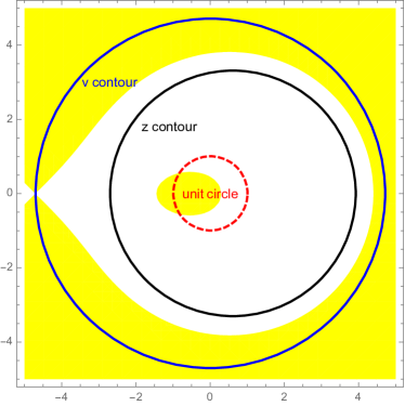
Refer to caption
Refer to caption
Figure 7: The plot exemplifies steepest descent deformations for the frozen (left) and empty (right) regions. The yellow region again signifies the region โ„œโ€‹((Sโ€‹(v)โˆ’Sโ€‹(z0)))>0โ„œ๐‘†๐‘ฃ๐‘†subscript๐‘ง00\mathfrak{R}((S(v)-S(z_{0})))>0 and the white elsewhere.

For the case (ฯ„,ฮฝ,ฮท)โˆˆ๐’Ÿfโ€‹rโ€‹oโ€‹zโ€‹eโ€‹n๐œ๐œˆ๐œ‚superscript๐’Ÿ๐‘“๐‘Ÿ๐‘œ๐‘ง๐‘’๐‘›(\tau,\nu,\eta)\in\mathcal{D}^{frozen}, do not deform the initial u๐‘ขu contour and only make the substitutions x=(z+zโˆ’1)/2๐‘ฅ๐‘งsuperscript๐‘ง12x=(z+z^{-1})/2, u=(v+vโˆ’1)/2๐‘ข๐‘ฃsuperscript๐‘ฃ12u=(v+v^{-1})/2, as before. Steepest descent deformations as in the plot of Figure 7 do not produce residues at v=zโˆ’1๐‘ฃsuperscript๐‘ง1v=z^{-1} since z0โ€‹(ฯ„,ฮฝ,ฮท)=zmโ€‹iโ€‹n<โˆ’1subscript๐‘ง0๐œ๐œˆ๐œ‚subscript๐‘ง๐‘š๐‘–๐‘›1z_{0}(\tau,\nu,\eta)=z_{min}<-1 and also no residues at v=z๐‘ฃ๐‘งv=z by considering the indicated regions of the plot. Hence, the double contour vanishes as Nโ†’โˆžโ†’๐‘N\to\infty without leaving behind any terms and we are left with the triangular matrix governed by the first term in Lemma 6.1:

1(nโ‰ฅm)โ€‹2rmโˆ’rnโ€‹(โˆ’1)ฮฑnโˆ’ฮฑm2โ€‹ฯ€โ€‹iโ€‹โˆฎ|z|=1z(t+rm+ฮฑm)โˆ’(s+rn+ฮฑn)โˆ’1โ€‹(1โˆ’z)nโˆ’mโ€‹๐‘‘z.subscript1๐‘›๐‘šsuperscript2subscript๐‘Ÿ๐‘šsubscript๐‘Ÿ๐‘›superscript1subscript๐›ผ๐‘›subscript๐›ผ๐‘š2๐œ‹๐‘–subscriptcontour-integral๐‘ง1superscript๐‘ง๐‘กsubscript๐‘Ÿ๐‘šsubscript๐›ผ๐‘š๐‘ subscript๐‘Ÿ๐‘›subscript๐›ผ๐‘›1superscript1๐‘ง๐‘›๐‘šdifferential-d๐‘ง1_{(n\geq m)}\frac{2^{r_{m}-r_{n}}(-1)^{\alpha_{n}-\alpha_{m}}}{2\pi i}\oint_{|z|=1}z^{(t+r_{m}+\alpha_{m})-(s+r_{n}+\alpha_{n})-1}(1-z)^{n-m}dz.

Since the diagonal entries of this triangular matrix are 111, the determinant of Kฮณsuperscript๐พ๐›พK^{\gamma} converges to 111. This confirms the definition of ๐’Ÿfโ€‹rโ€‹oโ€‹zโ€‹eโ€‹nsuperscript๐’Ÿ๐‘“๐‘Ÿ๐‘œ๐‘ง๐‘’๐‘›\mathcal{D}^{frozen}.

Finally, for (ฯ„,ฮฝ,ฮท)โˆˆ๐’Ÿeโ€‹mโ€‹pโ€‹tโ€‹y๐œ๐œˆ๐œ‚superscript๐’Ÿ๐‘’๐‘š๐‘๐‘ก๐‘ฆ(\tau,\nu,\eta)\in\mathcal{D}^{empty}, again refrain from deforming the initial u๐‘ขu contour, but make the substitutions x=(z+zโˆ’1)/2๐‘ฅ๐‘งsuperscript๐‘ง12x=(z+z^{-1})/2, u=(v+vโˆ’1)/2๐‘ข๐‘ฃsuperscript๐‘ฃ12u=(v+v^{-1})/2, as before. We may perform the same calculation leading to (68), but now the transformation vโ†’vโˆ’1โ†’๐‘ฃsuperscript๐‘ฃ1v\to v^{-1} to the second summand at the end of (68) leads to a loop inside the unit circle (currently the z๐‘งz contour). This second summand disappears without leaving anything behind since we may shrink its v๐‘ฃv-loop arbitrarily to avoid residues at v=zโˆ’1๐‘ฃsuperscript๐‘ง1v=z^{-1} while making z๐‘งz-deformations as in Figure 7. But these deformations in the first summand of (68) leave behind a full loop of residues at v=z๐‘ฃ๐‘งv=z similar to (71) and Lemma 6.3:

โˆ’2rmโˆ’rnโ€‹(โˆ’1)ฮฑnโˆ’ฮฑm2โ€‹ฯ€โ€‹iโ€‹โˆฎ|z|=1z(t+rm+ฮฑm)โˆ’(s+rn+ฮฑn)โˆ’1โ€‹(1โˆ’z)nโˆ’mโ€‹๐‘‘z,superscript2subscript๐‘Ÿ๐‘šsubscript๐‘Ÿ๐‘›superscript1subscript๐›ผ๐‘›subscript๐›ผ๐‘š2๐œ‹๐‘–subscriptcontour-integral๐‘ง1superscript๐‘ง๐‘กsubscript๐‘Ÿ๐‘šsubscript๐›ผ๐‘š๐‘ subscript๐‘Ÿ๐‘›subscript๐›ผ๐‘›1superscript1๐‘ง๐‘›๐‘šdifferential-d๐‘ง-\frac{2^{r_{m}-r_{n}}(-1)^{\alpha_{n}-\alpha_{m}}}{2\pi i}\oint_{|z|=1}z^{(t+r_{m}+\alpha_{m})-(s+r_{n}+\alpha_{n})-1}(1-z)^{n-m}dz,

Since we did not perform any deformations to the initial u๐‘ขu contour, we are asymptotically left with the sum of this last residue and the first term in Lemma 6.1:

โˆ’1(n<m)โ€‹2rmโˆ’rnโ€‹(โˆ’1)ฮฑnโˆ’ฮฑm2โ€‹ฯ€โ€‹iโ€‹โˆฎ|z|=1z(t+rm+ฮฑm)โˆ’(s+rn+ฮฑn)โˆ’1โ€‹(1โˆ’z)nโˆ’mโ€‹๐‘‘zsubscript1๐‘›๐‘šsuperscript2subscript๐‘Ÿ๐‘šsubscript๐‘Ÿ๐‘›superscript1subscript๐›ผ๐‘›subscript๐›ผ๐‘š2๐œ‹๐‘–subscriptcontour-integral๐‘ง1superscript๐‘ง๐‘กsubscript๐‘Ÿ๐‘šsubscript๐›ผ๐‘š๐‘ subscript๐‘Ÿ๐‘›subscript๐›ผ๐‘›1superscript1๐‘ง๐‘›๐‘šdifferential-d๐‘ง-1_{(n<m)}\frac{2^{r_{m}-r_{n}}(-1)^{\alpha_{n}-\alpha_{m}}}{2\pi i}\oint_{|z|=1}z^{(t+r_{m}+\alpha_{m})-(s+r_{n}+\alpha_{n})-1}(1-z)^{n-m}dz

Since the diagonal entries of this triangular matrix are 00, the determinant of Kฮณsuperscript๐พ๐›พK^{\gamma} converges to 00. This confirms the definition of ๐’Ÿeโ€‹mโ€‹pโ€‹tโ€‹ysuperscript๐’Ÿ๐‘’๐‘š๐‘๐‘ก๐‘ฆ\mathcal{D}^{empty}.

6.2 Edge limits

6.2.1 Finite distance from the wall: Jacobi kernel

Assume again that ฮณโˆผNโ‹…ฯ„>0similar-to๐›พโ‹…๐‘๐œ0\gamma\sim N\cdot\tau>0 and rn,rmโˆผNโ‹…ฮท>0similar-tosubscript๐‘Ÿ๐‘›subscript๐‘Ÿ๐‘šโ‹…๐‘๐œ‚0r_{n},r_{m}\sim N\cdot\eta>0, but that s,t๐‘ ๐‘กs,t are fixed and finite. Assume only the difference nโˆ’m๐‘›๐‘šn-m is of constant order. Let Aโ€‹(z):=ฯ„โ€‹z+ฮทโ€‹logโก(1โˆ’z)assign๐ด๐‘ง๐œ๐‘ง๐œ‚1๐‘งA(z):=\tau z+\eta\log(1-z) and note 1โˆ’ฮท/ฯ„1๐œ‚๐œ1-\eta/\tau is a zero of Aโ€ฒโ€‹(z)superscript๐ดโ€ฒ๐‘งA^{\prime}(z). Write our kernel as

2ฮฑn+1/2ฯ€โ€‹12โ€‹ฯ€โ€‹isuperscript2subscript๐›ผ๐‘›12๐œ‹12๐œ‹๐‘–\displaystyle\frac{2^{\alpha_{n}+1/2}}{\pi}\frac{1}{2\pi i} โˆซโˆ’11โˆฎeโˆ’Nโ€‹(Aโ€‹(1โˆ’ฮท/ฯ„)โˆ’Aโ€‹(x))eNโ€‹(Aโ€‹(u)โˆ’Aโ€‹(1โˆ’ฮท/ฯ„))โ€‹Js,ฮฑnโ€‹(x)โ€‹Jt,ฮฑmโ€‹(u)โ€‹(xโˆ’1)rn(uโˆ’1)rmโ€‹(1โˆ’x)ฮฑnโ€‹(1+x)1/2xโˆ’uโ€‹๐‘‘uโ€‹๐‘‘xsuperscriptsubscript11contour-integralsuperscript๐‘’๐‘๐ด1๐œ‚๐œ๐ด๐‘ฅsuperscript๐‘’๐‘๐ด๐‘ข๐ด1๐œ‚๐œsubscript๐ฝ๐‘ subscript๐›ผ๐‘›๐‘ฅsubscript๐ฝ๐‘กsubscript๐›ผ๐‘š๐‘ขsuperscript๐‘ฅ1subscript๐‘Ÿ๐‘›superscript๐‘ข1subscript๐‘Ÿ๐‘šsuperscript1๐‘ฅsubscript๐›ผ๐‘›superscript1๐‘ฅ12๐‘ฅ๐‘ขdifferential-d๐‘ขdifferential-d๐‘ฅ\displaystyle\int_{-1}^{1}\oint\frac{e^{-N(A(1-\eta/\tau)-A(x))}}{e^{N(A(u)-A(1-\eta/\tau))}}J_{s,\alpha_{n}}(x)J_{t,\alpha_{m}}(u)\frac{(x-1)^{r_{n}}}{(u-1)^{r_{m}}}\frac{(1-x)^{\alpha_{n}}(1+x)^{1/2}}{x-u}dudx
+1(nโ‰ฅm)โ€‹โŸจJs,ฮฑn,(xโˆ’1)rnโˆ’rmโ€‹Jt,ฮฑmโŸฉฮฑn.subscript1๐‘›๐‘šsubscriptsubscript๐ฝ๐‘ subscript๐›ผ๐‘›superscript๐‘ฅ1subscript๐‘Ÿ๐‘›subscript๐‘Ÿ๐‘šsubscript๐ฝ๐‘กsubscript๐›ผ๐‘šsubscript๐›ผ๐‘›\displaystyle+1_{(n\geq m)}\left\langle J_{s,\alpha_{n}},(x-1)^{r_{n}-r_{m}}J_{t,\alpha_{m}}\right\rangle_{\alpha_{n}}.
Refer to caption
Figure 8: The plot exemplifies steepest descent deformations when targeting a finite distance from the wall. The yellow region signifies where โ„œโ€‹(Aโ€‹(u)โˆ’Aโ€‹(1โˆ’ฮท/ฯ„))>0โ„œ๐ด๐‘ข๐ด1๐œ‚๐œ0\mathfrak{R}(A(u)-A(1-\eta/\tau))>0 and the white elsewhere.

Now deform the u๐‘ขu-contour, as in Figure 8, to be a steepest ascent loop remaining in the region โ„›โ€‹(Aโ€‹(u)โˆ’Aโ€‹(1โˆ’ฮท/ฯ„))>0โ„›๐ด๐‘ข๐ด1๐œ‚๐œ0\mathcal{R}(A(u)-A(1-\eta/\tau))>0 and passing through the critical point 1โˆ’ฮท/ฯ„1๐œ‚๐œ1-\eta/\tau. If 1โˆ’ฮท/ฯ„<โˆ’11๐œ‚๐œ11-\eta/\tau<-1, the unit interval already lies in the region โ„›โ€‹(Aโ€‹(1โˆ’ฮท/ฯ„)โˆ’Aโ€‹(x))>0โ„›๐ด1๐œ‚๐œ๐ด๐‘ฅ0\mathcal{R}(A(1-\eta/\tau)-A(x))>0, so the double integral term tends to zero without picking up residues. As for the frozen region above, the kernel converges to a triangular matrix whose diagonal entries are 111โ€™s. But if 1โˆ’ฮท/ฯ„>โˆ’11๐œ‚๐œ11-\eta/\tau>-1, then we acquire a residue at u=x๐‘ข๐‘ฅu=x given by

โˆ’2ฮฑn+1/2โ€‹(โˆ’1)rnโˆ’rmฯ€โ€‹โˆซโˆ’11โˆ’ฮท/ฯ„Js,ฮฑnโ€‹(x)โ€‹Jt,ฮฑmโ€‹(x)โ€‹(1โˆ’x)rnโˆ’rm+ฮฑnโ€‹(1+x)1/2โ€‹๐‘‘xsuperscript2subscript๐›ผ๐‘›12superscript1subscript๐‘Ÿ๐‘›subscript๐‘Ÿ๐‘š๐œ‹superscriptsubscript11๐œ‚๐œsubscript๐ฝ๐‘ subscript๐›ผ๐‘›๐‘ฅsubscript๐ฝ๐‘กsubscript๐›ผ๐‘š๐‘ฅsuperscript1๐‘ฅsubscript๐‘Ÿ๐‘›subscript๐‘Ÿ๐‘šsubscript๐›ผ๐‘›superscript1๐‘ฅ12differential-d๐‘ฅ-\frac{2^{\alpha_{n}+1/2}(-1)^{r_{n}-r_{m}}}{\pi}\int_{-1}^{1-\eta/\tau}J_{s,\alpha_{n}}(x)J_{t,\alpha_{m}}(x)(1-x)^{r_{n}-r_{m}+\alpha_{n}}(1+x)^{1/2}dx

Noting that (โˆ’1)rnโˆ’rmsuperscript1subscript๐‘Ÿ๐‘›subscript๐‘Ÿ๐‘š(-1)^{r_{n}-r_{m}} is a conjugating factor completes the proof of Theorem 1.4.

6.2.2 Corner of phase transition: Pearcey kernel

Assume that ฮณโˆผN/2similar-to๐›พ๐‘2\gamma\sim N/2, and sโˆผN1/4โ€‹ฮฝ1>0similar-to๐‘ superscript๐‘14subscript๐œˆ10s\sim N^{1/4}\nu_{1}>0, tโˆผN1/4โ€‹ฮฝ2>0similar-to๐‘กsuperscript๐‘14subscript๐œˆ20t\sim N^{1/4}\nu_{2}>0, and lastly that rnโˆ’NโˆผNโ€‹ฮท1>0similar-tosubscript๐‘Ÿ๐‘›๐‘๐‘subscript๐œ‚10r_{n}-N\sim\sqrt{N}\eta_{1}>0, rmโˆ’NโˆผNโ€‹ฮท2>0similar-tosubscript๐‘Ÿ๐‘š๐‘๐‘subscript๐œ‚20r_{m}-N\sim\sqrt{N}\eta_{2}>0

Lemma 6.4.

Let x=Nโˆ’1/2โ€‹xโ€ฒโˆ’1โˆˆ[โˆ’1,1]๐‘ฅsuperscript๐‘12superscript๐‘ฅโ€ฒ111x=N^{-1/2}x^{\prime}-1\in[-1,1]. Then for large N๐‘N,

Nโˆ’1/4โ€‹(โˆ’1)sโ€‹Js,ฮฑโ€‹(x)โˆผsinโก[ฮฝ1โ€‹2โ€‹xโ€ฒ]2ฮฑโ€‹xโ€ฒ.similar-tosuperscript๐‘14superscript1๐‘ subscript๐ฝ๐‘ ๐›ผ๐‘ฅsubscript๐œˆ12superscript๐‘ฅโ€ฒsuperscript2๐›ผsuperscript๐‘ฅโ€ฒN^{-1/4}(-1)^{s}J_{s,\alpha}(x)\sim\frac{\sin[\nu_{1}\sqrt{2x^{\prime}}]}{2^{\alpha}\sqrt{x^{\prime}}}.
Proof.

Write x=cosโกฮธ๐‘ฅ๐œƒx=\cos\theta and note the power series

cosโˆ’1โก(zโˆ’1)=ฯ€โˆ’โˆซ0z12โ€‹xโ€‹1โˆ’x/2โ€‹๐‘‘x=ฯ€โˆ’2โ€‹z+212โ€‹z3/2+โ‹ฏ,superscript1๐‘ง1๐œ‹superscriptsubscript0๐‘ง12๐‘ฅ1๐‘ฅ2differential-d๐‘ฅ๐œ‹2๐‘ง212superscript๐‘ง32โ‹ฏ\cos^{-1}(z-1)=\pi-\int_{0}^{z}\frac{1}{\sqrt{2x}\sqrt{1-x/2}}dx=\pi-\sqrt{2}\sqrt{z}+\frac{\sqrt{2}}{12}z^{3/2}+\cdots,

If ฮฑ=โˆ’1/2๐›ผ12\alpha=-1/2, then by (32), Js,โˆ’1/2โ€‹(x)=cosโก(s+1/2)โ€‹ฮธcosโก(ฮธ/2)subscript๐ฝ๐‘ 12๐‘ฅ๐‘ 12๐œƒ๐œƒ2J_{s,-1/2}(x)=\frac{\cos(s+1/2)\theta}{\cos(\theta/2)} so that

(โˆ’1)sโ€‹Js,โˆ’1/2โ€‹(x)superscript1๐‘ subscript๐ฝ๐‘ 12๐‘ฅ\displaystyle(-1)^{s}J_{s,-1/2}(x) =(โˆ’1)sโ€‹cosโก[(s+1/2)โ€‹ฯ€โˆ’sโ€‹Nโˆ’1/4โ€‹2โ€‹xโ€ฒ+oโ€‹(1)]cosโก[ฯ€/2โˆ’Nโˆ’1/4โ€‹xโ€ฒ/2+oโ€‹(1)]absentsuperscript1๐‘ ๐‘ 12๐œ‹๐‘ superscript๐‘142superscript๐‘ฅโ€ฒ๐‘œ1๐œ‹2superscript๐‘14superscript๐‘ฅโ€ฒ2๐‘œ1\displaystyle=(-1)^{s}\frac{\cos[(s+1/2)\pi-sN^{-1/4}\sqrt{2x^{\prime}}+o(1)]}{\cos[\pi/2-N^{-1/4}\sqrt{x^{\prime}/2}+o(1)]}
=(โˆ’1)sโ€‹cosโก[(s+1/2)โ€‹ฯ€+oโ€‹(1)]โ€‹cosโก[ฮฝ1โ€‹2โ€‹xโ€ฒ]+sinโก[(s+1/2)โ€‹ฯ€+oโ€‹(1)]โ€‹sinโก[ฮฝ1โ€‹2โ€‹xโ€ฒ]cosโก[ฯ€/2+oโ€‹(1)]โ€‹cosโก[Nโˆ’1/4โ€‹xโ€ฒ/2]+sinโก[ฯ€/2+oโ€‹(1)]โ€‹sinโก[Nโˆ’1/4โ€‹xโ€ฒ/2]absentsuperscript1๐‘ ๐‘ 12๐œ‹๐‘œ1subscript๐œˆ12superscript๐‘ฅโ€ฒ๐‘ 12๐œ‹๐‘œ1subscript๐œˆ12superscript๐‘ฅโ€ฒ๐œ‹2๐‘œ1superscript๐‘14superscript๐‘ฅโ€ฒ2๐œ‹2๐‘œ1superscript๐‘14superscript๐‘ฅโ€ฒ2\displaystyle=(-1)^{s}\frac{\cos[(s+1/2)\pi+o(1)]\cos[\nu_{1}\sqrt{2x^{\prime}}]+\sin[(s+1/2)\pi+o(1)]\sin[\nu_{1}\sqrt{2x^{\prime}}]}{\cos[\pi/2+o(1)]\cos[N^{-1/4}\sqrt{x^{\prime}/2}]+\sin[\pi/2+o(1)]\sin[N^{-1/4}\sqrt{x^{\prime}/2}]}
โˆผsinโก[ฮฝ1โ€‹2โ€‹xโ€ฒ]sinโก[Nโˆ’1/4โ€‹xโ€ฒ/2],similar-toabsentsubscript๐œˆ12superscript๐‘ฅโ€ฒsuperscript๐‘14superscript๐‘ฅโ€ฒ2\displaystyle\sim\frac{\sin[\nu_{1}\sqrt{2x^{\prime}}]}{\sin[N^{-1/4}\sqrt{x^{\prime}/2}]},

and we may similarly use Js,1/2โ€‹(x)=sinโก(s+1)โ€‹ฮธsinโกฮธsubscript๐ฝ๐‘ 12๐‘ฅ๐‘ 1๐œƒ๐œƒJ_{s,1/2}(x)=\frac{\sin(s+1)\theta}{\sin\theta} if ฮฑ=1/2๐›ผ12\alpha=1/2. Using limyโ†’0ysinโกy=1subscriptโ†’๐‘ฆ0๐‘ฆ๐‘ฆ1\lim_{y\to 0}\frac{y}{\sin y}=1 completes the proof. โˆŽ

Recall for any ฯ‰=(ฮฑ,ฮฒ,ฮณ)๐œ”๐›ผ๐›ฝ๐›พ\omega=(\alpha,\beta,\gamma), the complementary point process (๐’ณ~ฯ‰)csuperscriptsuperscript~๐’ณ๐œ”๐‘(\widetilde{\mathcal{X}}^{\omega})^{c} of ๐’ณ~ฯ‰superscript~๐’ณ๐œ”\widetilde{\mathcal{X}}^{\omega} is also determinantal with k๐‘˜kth correlation function

ฯ~ฮ”ฯ‰,kโ€‹(z1,โ€ฆ,zk):=โ„™โ€‹((๐’ณ~ฯ‰)cโŠƒ{z1,โ€ฆ,zk})=det[Kฮ”ฯ‰โ€‹(zi,zj)]i,j=1k,assignsubscriptsuperscript~๐œŒ๐œ”๐‘˜ฮ”subscript๐‘ง1โ€ฆsubscript๐‘ง๐‘˜โ„™subscript๐‘ง1โ€ฆsubscript๐‘ง๐‘˜superscriptsuperscript~๐’ณ๐œ”๐‘superscriptsubscriptdelimited-[]superscriptsubscript๐พฮ”๐œ”subscript๐‘ง๐‘–subscript๐‘ง๐‘—๐‘–๐‘—1๐‘˜\widetilde{\rho}^{\omega,k}_{\Delta}(z_{1},\ldots,z_{k}):=\mathbb{P}\left((\widetilde{\mathcal{X}}^{\omega})^{c}\supset\{z_{1},\ldots,z_{k}\}\right)=\det[K_{\Delta}^{\omega}(z_{i},z_{j})]_{i,j=1}^{k},

where the kernel Kฮ”ฯ‰subscriptsuperscript๐พ๐œ”ฮ”K^{\omega}_{\Delta} is readily computable (using orthogonality for the Chebyshev polynomials) as

Kฮ”ฯ‰โ€‹((s,n),(t,m)):=โˆ’2ฮฑn+1/2ฯ€โ€‹12โ€‹ฯ€โ€‹iassignsubscriptsuperscript๐พ๐œ”ฮ”๐‘ ๐‘›๐‘ก๐‘šsuperscript2subscript๐›ผ๐‘›12๐œ‹12๐œ‹๐‘–\displaystyle K^{\omega}_{\Delta}((s,n),(t,m)):=-\frac{2^{\alpha_{n}+1/2}}{\pi}\frac{1}{2\pi i} โˆซโˆ’11โˆฎEฯ‰โ€‹(x)Eฯ‰โ€‹(u)โ€‹Js,ฮฑnโ€‹(x)โ€‹Jt,ฮฑmโ€‹(u)โ€‹(xโˆ’1)rn(uโˆ’1)rmโ€‹(1โˆ’x)ฮฑnโ€‹(1+x)1/2xโˆ’uโ€‹๐‘‘uโ€‹๐‘‘xsuperscriptsubscript11contour-integralsuperscript๐ธ๐œ”๐‘ฅsuperscript๐ธ๐œ”๐‘ขsubscript๐ฝ๐‘ subscript๐›ผ๐‘›๐‘ฅsubscript๐ฝ๐‘กsubscript๐›ผ๐‘š๐‘ขsuperscript๐‘ฅ1subscript๐‘Ÿ๐‘›superscript๐‘ข1subscript๐‘Ÿ๐‘šsuperscript1๐‘ฅsubscript๐›ผ๐‘›superscript1๐‘ฅ12๐‘ฅ๐‘ขdifferential-d๐‘ขdifferential-d๐‘ฅ\displaystyle\int_{-1}^{1}\oint\frac{E^{\omega}(x)}{E^{\omega}(u)}J_{s,\alpha_{n}}(x)J_{t,\alpha_{m}}(u)\frac{(x-1)^{r_{n}}}{(u-1)^{r_{m}}}\frac{(1-x)^{\alpha_{n}}(1+x)^{1/2}}{x-u}dudx (72)
โˆ’1(n>m)โ€‹โŸจJs,ฮฑn,(xโˆ’1)rnโˆ’rmโ€‹Jt,ฮฑmโŸฉฮฑn.subscript1๐‘›๐‘šsubscriptsubscript๐ฝ๐‘ subscript๐›ผ๐‘›superscript๐‘ฅ1subscript๐‘Ÿ๐‘›subscript๐‘Ÿ๐‘šsubscript๐ฝ๐‘กsubscript๐›ผ๐‘šsubscript๐›ผ๐‘›\displaystyle-1_{(n>m)}\left\langle J_{s,\alpha_{n}},(x-1)^{r_{n}-r_{m}}J_{t,\alpha_{m}}\right\rangle_{\alpha_{n}}.
Refer to caption
Figure 9: Steepest descent deformations when targeting the corner of the phase transition. The yellow region signifies the region โ„œโ€‹(Aโ€‹(u)โˆ’Aโ€‹(โˆ’1))>0โ„œ๐ด๐‘ข๐ด10\mathfrak{R}(A(u)-A(-1))>0 and the white elsewhere.

Deforming the u๐‘ขu-contour in the double integral term of (72) (with ฯ‰=(0,0,ฮณ)๐œ”00๐›พ\omega=(0,0,\gamma)) as in Figure 9, we endeavor to find the contribution at โˆ’11-1. Making the substitutions xโ€ฒ=N1/2โ€‹(x+1)superscript๐‘ฅโ€ฒsuperscript๐‘12๐‘ฅ1x^{\prime}=N^{1/2}(x+1) and uโ€ฒ=N1/2โ€‹(u+1)superscript๐‘ขโ€ฒsuperscript๐‘12๐‘ข1u^{\prime}=N^{1/2}(u+1), we have, for large N๐‘N,

(1โˆ’x)ฮฑnโ€‹(1+x)1/2xโˆ’uโ€‹dโ€‹uโ€‹dโ€‹xsuperscript1๐‘ฅsubscript๐›ผ๐‘›superscript1๐‘ฅ12๐‘ฅ๐‘ข๐‘‘๐‘ข๐‘‘๐‘ฅ\displaystyle\frac{(1-x)^{\alpha_{n}}(1+x)^{1/2}}{x-u}dudx =N1/2โ€‹(2โˆ’xโ€ฒโ€‹Nโˆ’1/2)ฮฑnโ€‹xโ€ฒโ€‹Nโˆ’1/4xโ€ฒโˆ’uโ€ฒโ‹…Nโˆ’1โ€‹dโ€‹uโ€ฒโ€‹dโ€‹xโ€ฒabsentโ‹…superscript๐‘12superscript2superscript๐‘ฅโ€ฒsuperscript๐‘12subscript๐›ผ๐‘›superscript๐‘ฅโ€ฒsuperscript๐‘14superscript๐‘ฅโ€ฒsuperscript๐‘ขโ€ฒsuperscript๐‘1๐‘‘superscript๐‘ขโ€ฒ๐‘‘superscript๐‘ฅโ€ฒ\displaystyle=N^{1/2}\frac{(2-x^{\prime}N^{-1/2})^{\alpha_{n}}\sqrt{x^{\prime}}N^{-1/4}}{x^{\prime}-u^{\prime}}\cdot N^{-1}du^{\prime}dx^{\prime}
โˆผNโˆ’3/4โ€‹2ฮฑnโ€‹xโ€ฒxโ€ฒโˆ’uโ€ฒโ‹…dโ€‹uโ€ฒโ€‹dโ€‹xโ€ฒ.similar-toabsentโ‹…superscript๐‘34superscript2subscript๐›ผ๐‘›superscript๐‘ฅโ€ฒsuperscript๐‘ฅโ€ฒsuperscript๐‘ขโ€ฒ๐‘‘superscript๐‘ขโ€ฒ๐‘‘superscript๐‘ฅโ€ฒ\displaystyle\sim N^{-3/4}\frac{2^{\alpha_{n}}\sqrt{x^{\prime}}}{x^{\prime}-u^{\prime}}\cdot du^{\prime}dx^{\prime}.

Putting this together with Lemma 6.4, we get

2ฮฑmโ€‹(โˆ’1)sโ€‹Js,ฮฑnโ€‹(x)โ€‹(โˆ’1)tโ€‹Jt,ฮฑmโ€‹(u)โ€‹(1โˆ’x)ฮฑnโ€‹(1+x)1/2xโˆ’uโ€‹dโ€‹uโ€‹dโ€‹xโˆผNโˆ’1/4โ€‹sinโก[ฮฝ1โ€‹2โ€‹xโ€ฒ]โ€‹sinโก[ฮฝ2โ€‹2โ€‹uโ€ฒ]โ€‹dโ€‹uโ€ฒโ€‹dโ€‹xโ€ฒuโ€ฒโ€‹(xโ€ฒโˆ’uโ€ฒ).similar-tosuperscript2subscript๐›ผ๐‘šsuperscript1๐‘ subscript๐ฝ๐‘ subscript๐›ผ๐‘›๐‘ฅsuperscript1๐‘กsubscript๐ฝ๐‘กsubscript๐›ผ๐‘š๐‘ขsuperscript1๐‘ฅsubscript๐›ผ๐‘›superscript1๐‘ฅ12๐‘ฅ๐‘ข๐‘‘๐‘ข๐‘‘๐‘ฅsuperscript๐‘14subscript๐œˆ12superscript๐‘ฅโ€ฒsubscript๐œˆ22superscript๐‘ขโ€ฒ๐‘‘superscript๐‘ขโ€ฒ๐‘‘superscript๐‘ฅโ€ฒsuperscript๐‘ขโ€ฒsuperscript๐‘ฅโ€ฒsuperscript๐‘ขโ€ฒ2^{\alpha_{m}}(-1)^{s}J_{s,\alpha_{n}}(x)(-1)^{t}J_{t,\alpha_{m}}(u)\frac{(1-x)^{\alpha_{n}}(1+x)^{1/2}}{x-u}dudx\sim N^{-1/4}\sin[\nu_{1}\sqrt{2x^{\prime}}]\sin[\nu_{2}\sqrt{2u^{\prime}}]\frac{du^{\prime}dx^{\prime}}{\sqrt{u^{\prime}}(x^{\prime}-u^{\prime})}.

The remainder of the integrand satisfies

(โˆ’1)rmโˆ’rnโ€‹2rmโˆ’rnโ€‹eฮณโ€‹xeฮณโ€‹uโ€‹(xโˆ’1)rn(uโˆ’1)rmsuperscript1subscript๐‘Ÿ๐‘šsubscript๐‘Ÿ๐‘›superscript2subscript๐‘Ÿ๐‘šsubscript๐‘Ÿ๐‘›superscript๐‘’๐›พ๐‘ฅsuperscript๐‘’๐›พ๐‘ขsuperscript๐‘ฅ1subscript๐‘Ÿ๐‘›superscript๐‘ข1subscript๐‘Ÿ๐‘š\displaystyle(-1)^{r_{m}-r_{n}}2^{r_{m}-r_{n}}\frac{e^{\gamma x}}{e^{\gamma u}}\frac{(x-1)^{r_{n}}}{(u-1)^{r_{m}}} =eโˆ’Nโ€‹(Aโ€‹(โˆ’1)โˆ’Aโ€‹(x))+ฮท1โ€‹Nโ€‹(logโก(1โˆ’x)โˆ’logโก2)eNโ€‹(Aโ€‹(u)โˆ’Aโ€‹(โˆ’1))+ฮท2โ€‹Nโ€‹(logโก(1โˆ’u)โˆ’logโก2)โˆผeโˆ’(xโ€ฒ)2/8โˆ’ฮท1โ€‹xโ€ฒ/2eโˆ’(uโ€ฒ)2/8โˆ’ฮท2โ€‹uโ€ฒ/2,absentsuperscript๐‘’๐‘๐ด1๐ด๐‘ฅsubscript๐œ‚1๐‘1๐‘ฅ2superscript๐‘’๐‘๐ด๐‘ข๐ด1subscript๐œ‚2๐‘1๐‘ข2similar-tosuperscript๐‘’superscriptsuperscript๐‘ฅโ€ฒ28subscript๐œ‚1superscript๐‘ฅโ€ฒ2superscript๐‘’superscriptsuperscript๐‘ขโ€ฒ28subscript๐œ‚2superscript๐‘ขโ€ฒ2\displaystyle=\frac{e^{-N(A(-1)-A(x))+\eta_{1}\sqrt{N}(\log(1-x)-\log 2)}}{e^{N(A(u)-A(-1))+\eta_{2}\sqrt{N}(\log(1-u)-\log 2)}}\sim\frac{e^{-(x^{\prime})^{2}/8-\eta_{1}x^{\prime}/2}}{e^{-(u^{\prime})^{2}/8-\eta_{2}u^{\prime}/2}},

where Aโ€‹(z):=z/2+logโก(1โˆ’z)assign๐ด๐‘ง๐‘ง21๐‘งA(z):=z/2+\log(1-z) and the last approximation follows from, respectively, second and first order Taylor expansions about โˆ’11-1. Hence, putting everything together, we have

N1/4โ€‹2ฮฑmโˆ’ฮฑnโ€‹(โˆ’2)rmโˆ’rnsuperscript๐‘14superscript2subscript๐›ผ๐‘šsubscript๐›ผ๐‘›superscript2subscript๐‘Ÿ๐‘šsubscript๐‘Ÿ๐‘›\displaystyle N^{1/4}2^{\alpha_{m}-\alpha_{n}}(-2)^{r_{m}-r_{n}} (โˆ’1)tโˆ’sโ€‹2ฮฑn+1/2ฯ€โ€‹12โ€‹ฯ€โ€‹iโ€‹โˆซโˆ’11โˆฎeฮณโ€‹xeฮณโ€‹uโ€‹Js,ฮฑnโ€‹(x)โ€‹Jt,ฮฑmโ€‹(u)โ€‹(xโˆ’1)rn(uโˆ’1)rmโ€‹(1โˆ’x)ฮฑnโ€‹(1+x)1/2uโˆ’xโ€‹๐‘‘uโ€‹๐‘‘xsuperscript1๐‘ก๐‘ superscript2subscript๐›ผ๐‘›12๐œ‹12๐œ‹๐‘–superscriptsubscript11contour-integralsuperscript๐‘’๐›พ๐‘ฅsuperscript๐‘’๐›พ๐‘ขsubscript๐ฝ๐‘ subscript๐›ผ๐‘›๐‘ฅsubscript๐ฝ๐‘กsubscript๐›ผ๐‘š๐‘ขsuperscript๐‘ฅ1subscript๐‘Ÿ๐‘›superscript๐‘ข1subscript๐‘Ÿ๐‘šsuperscript1๐‘ฅsubscript๐›ผ๐‘›superscript1๐‘ฅ12๐‘ข๐‘ฅdifferential-d๐‘ขdifferential-d๐‘ฅ\displaystyle(-1)^{t-s}\frac{2^{\alpha_{n}+1/2}}{\pi}\frac{1}{2\pi i}\int_{-1}^{1}\oint\frac{e^{\gamma x}}{e^{\gamma u}}J_{s,\alpha_{n}}(x)J_{t,\alpha_{m}}(u)\frac{(x-1)^{r_{n}}}{(u-1)^{r_{m}}}\frac{(1-x)^{\alpha_{n}}(1+x)^{1/2}}{u-x}dudx
โ†’2ฯ€โ€‹12โ€‹ฯ€โ€‹iโ€‹โˆฎโˆ’iโ€‹โˆžiโ€‹โˆžโˆซ0โˆže(uโ€ฒ)2โˆ’(xโ€ฒ)28+ฮท2โ€‹uโ€ฒโˆ’ฮท1โ€‹xโ€ฒ2โ€‹sinโก[ฮฝ1โ€‹2โ€‹xโ€ฒ]โ€‹sinโก[ฮฝ2โ€‹2โ€‹uโ€ฒ]โ€‹dโ€‹xโ€ฒโ€‹dโ€‹uโ€ฒuโ€ฒโ€‹(uโ€ฒโˆ’xโ€ฒ)โ†’absent2๐œ‹12๐œ‹๐‘–superscriptsubscriptcontour-integral๐‘–๐‘–superscriptsubscript0superscript๐‘’superscriptsuperscript๐‘ขโ€ฒ2superscriptsuperscript๐‘ฅโ€ฒ28subscript๐œ‚2superscript๐‘ขโ€ฒsubscript๐œ‚1superscript๐‘ฅโ€ฒ2subscript๐œˆ12superscript๐‘ฅโ€ฒsubscript๐œˆ22superscript๐‘ขโ€ฒ๐‘‘superscript๐‘ฅโ€ฒ๐‘‘superscript๐‘ขโ€ฒsuperscript๐‘ขโ€ฒsuperscript๐‘ขโ€ฒsuperscript๐‘ฅโ€ฒ\displaystyle\to\frac{\sqrt{2}}{\pi}\frac{1}{2\pi i}\oint_{-i\infty}^{i\infty}\int_{0}^{\infty}e^{\frac{(u^{\prime})^{2}-(x^{\prime})^{2}}{8}+\frac{\eta_{2}u^{\prime}-\eta_{1}x^{\prime}}{2}}\sin[\nu_{1}\sqrt{2x^{\prime}}]\sin[\nu_{2}\sqrt{2u^{\prime}}]\frac{dx^{\prime}du^{\prime}}{\sqrt{u^{\prime}}(u^{\prime}-x^{\prime})}

Turning to the other term of Kฮ”ฮณsubscriptsuperscript๐พ๐›พฮ”K^{\gamma}_{\Delta}, note the following two asymptotic relations:

(โˆ’2)rmโˆ’rnโ€‹(xโˆ’1)rnโˆ’rm=(1โˆ’xโ€ฒ2โ€‹N)(ฮท1โˆ’ฮท2)โ€‹Nโ†’eโˆ’(ฮท1โˆ’ฮท2)โ€‹xโ€ฒ2.superscript2subscript๐‘Ÿ๐‘šsubscript๐‘Ÿ๐‘›superscript๐‘ฅ1subscript๐‘Ÿ๐‘›subscript๐‘Ÿ๐‘šsuperscript1superscript๐‘ฅโ€ฒ2๐‘subscript๐œ‚1subscript๐œ‚2๐‘โ†’superscript๐‘’subscript๐œ‚1subscript๐œ‚2superscript๐‘ฅโ€ฒ2(-2)^{r_{m}-r_{n}}(x-1)^{r_{n}-r_{m}}=\left(1-\frac{x^{\prime}}{2\sqrt{N}}\right)^{(\eta_{1}-\eta_{2})\sqrt{N}}\to e^{\frac{-(\eta_{1}-\eta_{2})x^{\prime}}{2}}.
2ฮฑmโ€‹(โˆ’1)sโ€‹Js,ฮฑnโ€‹(x)โ€‹(โˆ’1)tโ€‹Jt,ฮฑmโ€‹(x)โ€‹(1โˆ’x)ฮฑnโ€‹(1+x)1/2โ€‹dโ€‹xโˆผNโˆ’1/4โ€‹sinโก[ฮฝ1โ€‹2โ€‹xโ€ฒ]โ€‹sinโก[ฮฝ2โ€‹2โ€‹xโ€ฒ]โ€‹dโ€‹xโ€ฒxโ€ฒ.similar-tosuperscript2subscript๐›ผ๐‘šsuperscript1๐‘ subscript๐ฝ๐‘ subscript๐›ผ๐‘›๐‘ฅsuperscript1๐‘กsubscript๐ฝ๐‘กsubscript๐›ผ๐‘š๐‘ฅsuperscript1๐‘ฅsubscript๐›ผ๐‘›superscript1๐‘ฅ12๐‘‘๐‘ฅsuperscript๐‘14subscript๐œˆ12superscript๐‘ฅโ€ฒsubscript๐œˆ22superscript๐‘ฅโ€ฒ๐‘‘superscript๐‘ฅโ€ฒsuperscript๐‘ฅโ€ฒ2^{\alpha_{m}}(-1)^{s}J_{s,\alpha_{n}}(x)(-1)^{t}J_{t,\alpha_{m}}(x)(1-x)^{\alpha_{n}}(1+x)^{1/2}dx\sim N^{-1/4}\sin[\nu_{1}\sqrt{2x^{\prime}}]\sin[\nu_{2}\sqrt{2x^{\prime}}]\frac{dx^{\prime}}{\sqrt{x^{\prime}}}.

Then the single integral term satisfies

N1/4superscript๐‘14\displaystyle N^{1/4} 2ฮฑmโˆ’ฮฑnโ€‹(โˆ’2)rmโˆ’rnโ€‹(โˆ’1)tโˆ’sโ€‹(โˆ’1(n>m)โ€‹โŸจJs,ฮฑn,(xโˆ’1)rnโˆ’rmโ€‹Jt,ฮฑmโŸฉฮฑn)superscript2subscript๐›ผ๐‘šsubscript๐›ผ๐‘›superscript2subscript๐‘Ÿ๐‘šsubscript๐‘Ÿ๐‘›superscript1๐‘ก๐‘ subscript1๐‘›๐‘šsubscriptsubscript๐ฝ๐‘ subscript๐›ผ๐‘›superscript๐‘ฅ1subscript๐‘Ÿ๐‘›subscript๐‘Ÿ๐‘šsubscript๐ฝ๐‘กsubscript๐›ผ๐‘šsubscript๐›ผ๐‘›\displaystyle 2^{\alpha_{m}-\alpha_{n}}(-2)^{r_{m}-r_{n}}(-1)^{t-s}\left(-1_{(n>m)}\left\langle J_{s,\alpha_{n}},(x-1)^{r_{n}-r_{m}}J_{t,\alpha_{m}}\right\rangle_{\alpha_{n}}\right)
โ†’1(ฮท1>ฮท2)โ€‹(โˆ’2ฯ€โ€‹โˆซ0โˆžeโˆ’(ฮท1โˆ’ฮท2)โ€‹xโ€ฒ2โ€‹sinโก[ฮฝ1โ€‹2โ€‹xโ€ฒ]โ€‹sinโก[ฮฝ2โ€‹2โ€‹xโ€ฒ]โ€‹dโ€‹xโ€ฒxโ€ฒ)โ†’absentsubscript1subscript๐œ‚1subscript๐œ‚22๐œ‹superscriptsubscript0superscript๐‘’subscript๐œ‚1subscript๐œ‚2superscript๐‘ฅโ€ฒ2subscript๐œˆ12superscript๐‘ฅโ€ฒsubscript๐œˆ22superscript๐‘ฅโ€ฒ๐‘‘superscript๐‘ฅโ€ฒsuperscript๐‘ฅโ€ฒ\displaystyle\to 1_{(\eta_{1}>\eta_{2})}\left(-\frac{\sqrt{2}}{\pi}\int_{0}^{\infty}e^{\frac{-(\eta_{1}-\eta_{2})x^{\prime}}{2}}\sin[\nu_{1}\sqrt{2x^{\prime}}]\sin[\nu_{2}\sqrt{2x^{\prime}}]\frac{dx^{\prime}}{\sqrt{x^{\prime}}}\right)
=1(ฮท1>ฮท2)โ€‹(12โ€‹ฯ€โ€‹โˆซ0โˆžeโˆ’(ฮท1โˆ’ฮท2)โ€‹xโ€ฒ2โ€‹[cosโก[(ฮฝ1+ฮฝ2)โ€‹2โ€‹xโ€ฒ]โˆ’cosโก[(ฮฝ1โˆ’ฮฝ2)โ€‹2โ€‹xโ€ฒ]]โ€‹dโ€‹xโ€ฒxโ€ฒ)absentsubscript1subscript๐œ‚1subscript๐œ‚212๐œ‹superscriptsubscript0superscript๐‘’subscript๐œ‚1subscript๐œ‚2superscript๐‘ฅโ€ฒ2delimited-[]subscript๐œˆ1subscript๐œˆ22superscript๐‘ฅโ€ฒsubscript๐œˆ1subscript๐œˆ22superscript๐‘ฅโ€ฒ๐‘‘superscript๐‘ฅโ€ฒsuperscript๐‘ฅโ€ฒ\displaystyle=1_{(\eta_{1}>\eta_{2})}\left(\frac{1}{\sqrt{2}\pi}\int_{0}^{\infty}e^{\frac{-(\eta_{1}-\eta_{2})x^{\prime}}{2}}\left[\cos[(\nu_{1}+\nu_{2})\sqrt{2x^{\prime}}]-\cos[(\nu_{1}-\nu_{2})\sqrt{2x^{\prime}}]\right]\frac{dx^{\prime}}{\sqrt{x^{\prime}}}\right)
=1(ฮท1>ฮท2)โ€‹1ฯ€โ€‹(ฮท1โˆ’ฮท2)โ€‹(expโก[โˆ’(ฮฝ1+ฮฝ2)2ฮท1โˆ’ฮท2]โˆ’expโก[โˆ’(ฮฝ1โˆ’ฮฝ2)2ฮท1โˆ’ฮท2]).absentsubscript1subscript๐œ‚1subscript๐œ‚21๐œ‹subscript๐œ‚1subscript๐œ‚2superscriptsubscript๐œˆ1subscript๐œˆ22subscript๐œ‚1subscript๐œ‚2superscriptsubscript๐œˆ1subscript๐œˆ22subscript๐œ‚1subscript๐œ‚2\displaystyle=1_{(\eta_{1}>\eta_{2})}\frac{1}{\sqrt{\pi(\eta_{1}-\eta_{2})}}\left(\exp\left[-\frac{(\nu_{1}+\nu_{2})^{2}}{\eta_{1}-\eta_{2}}\right]-\exp\left[-\frac{(\nu_{1}-\nu_{2})^{2}}{\eta_{1}-\eta_{2}}\right]\right).

where the last equality follows from standard Gaussian computations. Noting that the conjugating factors will disappear in the determinant completes the proof of Theorem 1.5.

Appendix A Algebraic argument for determinantal correlations

For completeness, this section covers the linear algebraic details on which Proposition 4.2 relies; we follow a combination of Theorem 4.2 of [9] and Lemma 3.4 of [11], which in turn rely on the Eynard-Mehta theorem in the manner of [18].

Fix nโ‰ฅ1๐‘›1n\geq 1. For 1โ‰คmโ‰คn1๐‘š๐‘›1\leq m\leq n and Nโˆˆโ„คโ‰ฅ0๐‘subscriptโ„คabsent0N\in\mathbb{Z}_{\geq 0}, consider point sets ๐”›(m):={xkm}k=1rmassignsuperscript๐”›๐‘šsuperscriptsubscriptsubscriptsuperscript๐‘ฅ๐‘š๐‘˜๐‘˜1subscript๐‘Ÿ๐‘š\mathfrak{X}^{(m)}:=\{x^{m}_{k}\}_{k=1}^{r_{m}} of variables xkmsubscriptsuperscript๐‘ฅ๐‘š๐‘˜x^{m}_{k} ranging in {0,โ€ฆ,N}0โ€ฆ๐‘\{0,\ldots,N\}, where we suppress dependence on N๐‘N. Define ๐”œ:=โˆชm=1n๐”›(m)assign๐”œsuperscriptsubscript๐‘š1๐‘›superscript๐”›๐‘š\mathfrak{Y}:=\cup_{m=1}^{n}\mathfrak{X}^{(m)} and recall our work in Section 4.2 furnishes a measure on point configurations in ๐”œ๐”œ\mathfrak{Y} up to level n๐‘›n by

constโ‹…โˆm=1nโˆ’1det[ฯ•mโ€‹(xim,xjm+1)]i,j=1rm+1โ‹…det[ฮจrnโˆ’jnโ€‹(xin)]i,j=1rn.โ‹…constsuperscriptsubscriptproduct๐‘š1๐‘›1โ‹…superscriptsubscriptdelimited-[]subscriptitalic-ฯ•๐‘šsubscriptsuperscript๐‘ฅ๐‘š๐‘–subscriptsuperscript๐‘ฅ๐‘š1๐‘—๐‘–๐‘—1subscript๐‘Ÿ๐‘š1superscriptsubscriptdelimited-[]subscriptsuperscriptฮจ๐‘›subscript๐‘Ÿ๐‘›๐‘—subscriptsuperscript๐‘ฅ๐‘›๐‘–๐‘–๐‘—1subscript๐‘Ÿ๐‘›\displaystyle\text{const}\cdot\prod_{m=1}^{n-1}\det\left[\phi_{m}(x^{m}_{i},x^{m+1}_{j})\right]_{i,j=1}^{r_{m+1}}\cdot\det\left[\Psi^{n}_{r_{n}-j}(x^{n}_{i})\right]_{i,j=1}^{r_{n}}. (73)

Note (73) uses our notational convention xrm+1mโ‰กโˆ’1subscriptsuperscript๐‘ฅ๐‘šsubscript๐‘Ÿ๐‘š11x^{m}_{r_{m+1}}\equiv-1 for m๐‘šm even (recall the proof of Lemma 3.4), so add the virtual variables ๐’ฑ:={viโ‰กโˆ’1}i=1rnassign๐’ฑsuperscriptsubscriptsubscript๐‘ฃ๐‘–1๐‘–1subscript๐‘Ÿ๐‘›\mathcal{V}:=\{v_{i}\equiv-1\}_{i=1}^{r_{n}} as a notational device to form the larger space ๐”›:=๐’ฑโˆช๐”œassign๐”›๐’ฑ๐”œ\mathfrak{X}:=\mathcal{V}\cup\mathfrak{Y}. To separate these variables out, let Wmsubscript๐‘Š๐‘šW_{m}, 1โ‰คmโ‰คnโˆ’11๐‘š๐‘›11\leq m\leq n-1, be the ๐”›(m)ร—๐”›(m+1)superscript๐”›๐‘šsuperscript๐”›๐‘š1\mathfrak{X}^{(m)}\times\mathfrak{X}^{(m+1)} matrix with entries Wmโ€‹(xim,xjm+1):=ฯ•mโ€‹(xim,xjm+1)assignsubscript๐‘Š๐‘šsubscriptsuperscript๐‘ฅ๐‘š๐‘–subscriptsuperscript๐‘ฅ๐‘š1๐‘—subscriptitalic-ฯ•๐‘šsubscriptsuperscript๐‘ฅ๐‘š๐‘–subscriptsuperscript๐‘ฅ๐‘š1๐‘—W_{m}(x^{m}_{i},x^{m+1}_{j}):=\phi_{m}(x^{m}_{i},x^{m+1}_{j}), and similarly, for 1โ‰คmโ‰คn1๐‘š๐‘›1\leq m\leq n, define a ๐’ฑร—๐”›(m)๐’ฑsuperscript๐”›๐‘š\mathcal{V}\times\mathfrak{X}^{(m)} matrix Emโˆ’1subscript๐ธ๐‘š1E_{m-1} to have entries Emโˆ’1โ€‹(vi,xjm)=ฯ•mโˆ’1โ€‹(vi,xjm)โ€‹1(i=rm)โ€‹1(m odd)subscript๐ธ๐‘š1subscript๐‘ฃ๐‘–subscriptsuperscript๐‘ฅ๐‘š๐‘—subscriptitalic-ฯ•๐‘š1subscript๐‘ฃ๐‘–subscriptsuperscript๐‘ฅ๐‘š๐‘—subscript1๐‘–subscript๐‘Ÿ๐‘šsubscript1m oddE_{m-1}(v_{i},x^{m}_{j})=\phi_{m-1}(v_{i},x^{m}_{j})1_{(i=r_{m})}1_{(\text{m odd})}. Define a ๐”›(k)ร—๐’ฑsuperscript๐”›๐‘˜๐’ฑ\mathfrak{X}^{(k)}\times\mathcal{V} matrix ๐šฟksuperscript๐šฟ๐‘˜\mathbf{\Psi}^{k} to have entries ๐šฟkโ€‹(xik,vj):=ฮจrkโˆ’jkโ€‹(xik)=โŸจJxik,ฮฑk,(xโˆ’1)rkโˆ’iโ€‹Riโˆ’rkEฯ‰โŸฉฮฑkassignsuperscript๐šฟ๐‘˜subscriptsuperscript๐‘ฅ๐‘˜๐‘–subscript๐‘ฃ๐‘—subscriptsuperscriptฮจ๐‘˜subscript๐‘Ÿ๐‘˜๐‘—subscriptsuperscript๐‘ฅ๐‘˜๐‘–subscriptsubscript๐ฝsubscriptsuperscript๐‘ฅ๐‘˜๐‘–subscript๐›ผ๐‘˜superscript๐‘ฅ1subscript๐‘Ÿ๐‘˜๐‘–subscriptsuperscript๐‘…superscript๐ธ๐œ”๐‘–subscript๐‘Ÿ๐‘˜subscript๐›ผ๐‘˜\mathbf{\Psi}^{k}(x^{k}_{i},v_{j}):=\Psi^{k}_{r_{k}-j}(x^{k}_{i})=\langle J_{x^{k}_{i},\alpha_{k}},(x-1)^{r_{k}-i}R^{E^{\omega}}_{i-r_{k}}\rangle_{\alpha_{k}}, as in Proposition 3.3.

Now the measure (73) is proportional to a minor of the ๐”›ร—๐”›๐”›๐”›\mathfrak{X}\times\mathfrak{X} matrix

L:=[0E00E2โ‹ฏEnโˆ’100โˆ’W10โ‹ฑ0000โˆ’W2โ‹ฑ0โ‹ฎโ‹ฑโ‹ฑโ‹ฑโ‹ฑโ‹ฎโ‹ฎโ‹ฑโ‹ฑโ‹ฑโ‹ฑโˆ’Wnโˆ’1๐šฟn00โ‹ฏ00]assign๐ฟmatrix0subscript๐ธ00subscript๐ธ2โ‹ฏsubscript๐ธ๐‘›100subscript๐‘Š10โ‹ฑ0000subscript๐‘Š2โ‹ฑ0โ‹ฎโ‹ฑโ‹ฑโ‹ฑโ‹ฑโ‹ฎโ‹ฎโ‹ฑโ‹ฑโ‹ฑโ‹ฑsubscript๐‘Š๐‘›1superscript๐šฟ๐‘›00โ‹ฏ00L:=\begin{bmatrix}0&E_{0}&0&E_{2}&\cdots&E_{n-1}\\ 0&0&-W_{1}&0&\ddots&0\\ 0&0&0&-W_{2}&\ddots&0\\ \vdots&\ddots&\ddots&\ddots&\ddots&\vdots\\ \vdots&\ddots&\ddots&\ddots&\ddots&-W_{n-1}\\ \mathbf{\Psi}^{n}&0&0&\cdots&0&0\end{bmatrix}

The matrix L๐ฟL supplies a point process (called an L-ensemble) on the larger space ๐”›๐”›\mathfrak{X} with distribution โ„™๐”›โ€‹(X):=detLXdet[I๐”›+L]assignsubscriptโ„™๐”›๐‘‹subscript๐ฟ๐‘‹delimited-[]subscript๐ผ๐”›๐ฟ\mathbb{P}_{\mathfrak{X}}(X):=\frac{\det L_{X}}{\det[I_{\mathfrak{X}}+L]}, Xโˆˆ2๐”›๐‘‹superscript2๐”›X\in 2^{\mathfrak{X}}, where LXsubscript๐ฟ๐‘‹L_{X} is the Xร—X๐‘‹๐‘‹X\times X submatrix and I๐”›:=I๐”›ร—๐”›assignsubscript๐ผ๐”›subscript๐ผ๐”›๐”›I_{\mathfrak{X}}:=I_{\mathfrak{X}\times\mathfrak{X}}. Its correlation function is determinantal with kernel K๐”›=I๐”›โˆ’(I๐”›+L)โˆ’1subscript๐พ๐”›subscript๐ผ๐”›superscriptsubscript๐ผ๐”›๐ฟ1K_{\mathfrak{X}}=I_{\mathfrak{X}}-(I_{\mathfrak{X}}+L)^{-1} (see [22]). Write I๐”œ+L=:[0ACD]I_{\mathfrak{Y}}+L=:\begin{bmatrix}0&A\\ C&D\end{bmatrix}, where as indicated, A๐ดA is the ๐’ฑร—๐”œ๐’ฑ๐”œ\mathcal{V}\times\mathfrak{Y} block, C๐ถC is the ๐”œร—๐’ฑ๐”œ๐’ฑ\mathfrak{Y}\times\mathcal{V} block, and D๐ทD the ๐”œร—๐”œ๐”œ๐”œ\mathfrak{Y}\times\mathfrak{Y} block. One can see by inspection that the ๐”œร—๐”œ๐”œ๐”œ\mathfrak{Y}\times\mathfrak{Y} matrix Dโˆ’1superscript๐ท1D^{-1} has (i,j)๐‘–๐‘—(i,j)-block W[i,j):=(W1โ€‹โ‹ฏโ€‹Wjโˆ’1)โ€‹1(i<j)+I๐”›(j)ร—๐”›(j)โ€‹1(i=j)assignsubscript๐‘Š๐‘–๐‘—subscript๐‘Š1โ‹ฏsubscript๐‘Š๐‘—1subscript1๐‘–๐‘—subscript๐ผsuperscript๐”›๐‘—superscript๐”›๐‘—subscript1๐‘–๐‘—W_{[i,j)}:=(W_{1}\cdots W_{j-1})1_{(i<j)}+I_{\mathfrak{X}^{(j)}\times\mathfrak{X}^{(j)}}1_{(i=j)}. Notice

Aโ€‹Dโˆ’1=(E0โ€‹W[1,1),โˆ‘k=12Ekโˆ’1โ€‹W[k,2),โˆ‘k=13Ekโˆ’1โ€‹W[k,3),โ€ฆ,โˆ‘k=1nEkโˆ’1โ€‹W[k,n))๐ดsuperscript๐ท1subscript๐ธ0subscript๐‘Š11superscriptsubscript๐‘˜12subscript๐ธ๐‘˜1subscript๐‘Š๐‘˜2superscriptsubscript๐‘˜13subscript๐ธ๐‘˜1subscript๐‘Š๐‘˜3โ€ฆsuperscriptsubscript๐‘˜1๐‘›subscript๐ธ๐‘˜1subscript๐‘Š๐‘˜๐‘›AD^{-1}=\left(E_{0}W_{[1,1)},\sum_{k=1}^{2}E_{k-1}W_{[k,2)},\sum_{k=1}^{3}E_{k-1}W_{[k,3)},\ldots,\sum_{k=1}^{n}E_{k-1}W_{[k,n)}\right)

Define also an rnร—rnsubscript๐‘Ÿ๐‘›subscript๐‘Ÿ๐‘›r_{n}\times r_{n} matrix Mn:=Aโ€‹Dโˆ’1โ€‹C=โˆ‘k=1nEkโˆ’1โ€‹W[k,n)โ€‹๐šฟnassignsubscript๐‘€๐‘›๐ดsuperscript๐ท1๐ถsuperscriptsubscript๐‘˜1๐‘›subscript๐ธ๐‘˜1subscript๐‘Š๐‘˜๐‘›superscript๐šฟ๐‘›M_{n}:=AD^{-1}C=\sum_{k=1}^{n}E_{k-1}W_{[k,n)}\mathbf{\Psi}^{n}.

Proposition A.1.

The point process of particle configurations up to level n๐‘›n governed by (73) is the same as the ๐”œ๐”œ\mathfrak{Y} conditional L๐ฟL-ensemble defined by the prescription โ„™๐”œโ€‹(Y):=detLYโˆช๐”œcdet[I๐”œ+L๐”œ]assignsubscriptโ„™๐”œ๐‘Œsubscript๐ฟ๐‘Œsuperscript๐”œ๐‘delimited-[]subscript๐ผ๐”œsubscript๐ฟ๐”œ\mathbb{P}_{\mathfrak{Y}}(Y):=\frac{\det L_{Y\cup\mathfrak{Y}^{c}}}{\det[I_{\mathfrak{Y}}+L_{\mathfrak{Y}}]}, Yโˆˆ2๐”›๐‘Œsuperscript2๐”›Y\in 2^{\mathfrak{X}}, which is determinantal with correlation kernel

K=I๐”œโˆ’(I๐”œ+L)โˆ’1|๐”œร—๐”œ=I๐”œโˆ’Dโˆ’1+Dโˆ’1โ€‹Cโ€‹Mnโˆ’1โ€‹Aโ€‹Dโˆ’1.๐พsubscript๐ผ๐”œevaluated-atsuperscriptsubscript๐ผ๐”œ๐ฟ1๐”œ๐”œsubscript๐ผ๐”œsuperscript๐ท1superscript๐ท1๐ถsuperscriptsubscript๐‘€๐‘›1๐ดsuperscript๐ท1K=I_{\mathfrak{Y}}-(I_{\mathfrak{Y}}+L)^{-1}|_{\mathfrak{Y}\times\mathfrak{Y}}=I_{\mathfrak{Y}}-D^{-1}+D^{-1}CM_{n}^{-1}AD^{-1}. (74)

More explicitly, its ๐”›(i)ร—๐”›(j)superscript๐”›๐‘–superscript๐”›๐‘—\mathfrak{X}^{(i)}\times\mathfrak{X}^{(j)}-block is given by

K(i,j):=K๐”›(i)ร—๐”›(j)=โˆ’W[i,j)โ€‹1(i<j)+[W[i,n)โ€‹๐šฟn]โ€‹[Mโˆ’1โ€‹(โˆ‘k=1jEkโˆ’1โ€‹W[k,j))].assignsubscript๐พ๐‘–๐‘—subscript๐พsuperscript๐”›๐‘–superscript๐”›๐‘—subscript๐‘Š๐‘–๐‘—subscript1๐‘–๐‘—delimited-[]subscript๐‘Š๐‘–๐‘›superscript๐šฟ๐‘›delimited-[]superscript๐‘€1superscriptsubscript๐‘˜1๐‘—subscript๐ธ๐‘˜1subscript๐‘Š๐‘˜๐‘—K_{(i,j)}:=K_{\mathfrak{X}^{(i)}\times\mathfrak{X}^{(j)}}=-W_{[i,j)}1_{(i<j)}+\left[W_{[i,n)}\mathbf{\Psi}^{n}\right]\left[M^{-1}\left(\sum_{k=1}^{j}E_{k-1}W_{[k,j)}\right)\right]. (75)
Proof.

For the the basic facts on conditional ensembles and in particular the first equality of (74), see [22]. The second equality is the content of the Eynardโ€“Mehta theorem, and is proved by computing the inverse of the 2ร—2222\times 2 block expression of I๐”œ+L=[0ACD]subscript๐ผ๐”œ๐ฟmatrix0๐ด๐ถ๐ทI_{\mathfrak{Y}}+L=\begin{bmatrix}0&A\\ C&D\end{bmatrix} in order to compute (I๐”œ+L)โˆ’1|๐”œร—๐”œevaluated-atsuperscriptsubscript๐ผ๐”œ๐ฟ1๐”œ๐”œ(I_{\mathfrak{Y}}+L)^{-1}|_{\mathfrak{Y}\times\mathfrak{Y}}. โˆŽ

Now let Nโ†’โˆžโ†’๐‘N\to\infty so that matrix multiplication induces convolution over โ„คโ‰ฅ0subscriptโ„คabsent0\mathbb{Z}_{\geq 0}, which is defined by (fโˆ—g)โ€‹(x,y):=โˆ‘zโ‰ฅ0fโ€‹(x,z)โ€‹gโ€‹(z,y)assign๐‘“๐‘”๐‘ฅ๐‘ฆsubscript๐‘ง0๐‘“๐‘ฅ๐‘ง๐‘”๐‘ง๐‘ฆ(f*g)(x,y):=\sum_{z\geq 0}f(x,z)g(z,y) for bivariate functions f,g๐‘“๐‘”f,g and by (fโˆ—g)โ€‹(x):=โˆ‘zโ‰ฅ0fโ€‹(x,z)โ€‹gโ€‹(z)assign๐‘“๐‘”๐‘ฅsubscript๐‘ง0๐‘“๐‘ฅ๐‘ง๐‘”๐‘ง(f*g)(x):=\sum_{z\geq 0}f(x,z)g(z) if g๐‘”g is univariate. We need to compute (75). Let ฯ•[i,n):=W[i,n)assignsuperscriptitalic-ฯ•๐‘–๐‘›subscript๐‘Š๐‘–๐‘›\phi^{[i,n)}:=W_{[i,n)} and note ฯ•[i,i):=I๐”›(i)assignsuperscriptitalic-ฯ•๐‘–๐‘–subscript๐ผsuperscript๐”›๐‘–\phi^{[i,i)}:=I_{\mathfrak{X}^{(i)}}. Then for each 1โ‰คjโ‰คn1๐‘—๐‘›1\leq j\leq n,

(โˆ‘k=1jEkโˆ’1โ€‹W[k,j))โ€‹(vs,xtj)=โˆ‘k=1j1(s=rk,kโ€‹oโ€‹dโ€‹d)โ€‹(ฯ•kโˆ’1โˆ—ฯ•[k,j))โ€‹(vk,xtj)=(ฯ•qsโˆ’1โˆ—ฯ•[qs,j))โ€‹(vs,xtj),superscriptsubscript๐‘˜1๐‘—subscript๐ธ๐‘˜1subscript๐‘Š๐‘˜๐‘—subscript๐‘ฃ๐‘ subscriptsuperscript๐‘ฅ๐‘—๐‘กsuperscriptsubscript๐‘˜1๐‘—subscript1๐‘ subscript๐‘Ÿ๐‘˜๐‘˜๐‘œ๐‘‘๐‘‘subscriptitalic-ฯ•๐‘˜1superscriptitalic-ฯ•๐‘˜๐‘—subscript๐‘ฃ๐‘˜subscriptsuperscript๐‘ฅ๐‘—๐‘กsubscriptitalic-ฯ•subscript๐‘ž๐‘ 1superscriptitalic-ฯ•subscript๐‘ž๐‘ ๐‘—subscript๐‘ฃ๐‘ subscriptsuperscript๐‘ฅ๐‘—๐‘ก\left(\sum_{k=1}^{j}E_{k-1}W_{[k,j)}\right)(v_{s},x^{j}_{t})=\sum_{k=1}^{j}1_{(s=r_{k},\ k\ odd)}(\phi_{k-1}*\phi^{[k,j)})(v_{k},x^{j}_{t})=(\phi_{q_{s}-1}*\phi^{[q_{s},j)})(v_{s},x^{j}_{t}), (76)

where qk:=2โ€‹kโˆ’1assignsubscript๐‘ž๐‘˜2๐‘˜1q_{k}:=2k-1. Take a ๐’ฑร—๐”›(j)๐’ฑsuperscript๐”›๐‘—\mathcal{V}\times\mathfrak{X}^{(j)} matrix ๐šฝjsuperscript๐šฝ๐‘—{\bf\Phi}^{j} with entries denoted ๐šฝj(vs,xtj)=:ฮฆrjโˆ’sj(xtj)1(sโ‰คrj){\bf\Phi}^{j}(v_{s},x^{j}_{t})=:\Phi^{j}_{r_{j}-s}(x^{j}_{t})1_{(s\leq r_{j})}, whose nonzero rows determine a basis for the row space {(ฯ•qsโˆ’1โˆ—ฯ•[qs,j))โ€‹(vs,x)|xโˆˆ๐”›(j)}s=1jsuperscriptsubscriptconditional-setsubscriptitalic-ฯ•subscript๐‘ž๐‘ 1superscriptitalic-ฯ•subscript๐‘ž๐‘ ๐‘—subscript๐‘ฃ๐‘ ๐‘ฅ๐‘ฅsuperscript๐”›๐‘—๐‘ 1๐‘—\{(\phi_{q_{s}-1}*\phi^{[q_{s},j)})(v_{s},x)|\ x\in\mathfrak{X}^{(j)}\}_{s=1}^{j} of (76), and which is biorthogonal to the ๐šฟisuperscript๐šฟ๐‘–{\bf\Psi}^{i} in the sense

โˆ‘kโ‰ฅ0ฮจrmโˆ’smโ€‹(k)โ€‹ฮฆrmโˆ’tmโ€‹(k)=ฮดsโ€‹t, 1โ‰คmโ‰คn.formulae-sequencesubscript๐‘˜0subscriptsuperscriptฮจ๐‘šsubscript๐‘Ÿ๐‘š๐‘ ๐‘˜subscriptsuperscriptฮฆ๐‘šsubscript๐‘Ÿ๐‘š๐‘ก๐‘˜subscript๐›ฟ๐‘ ๐‘ก1๐‘š๐‘›\sum_{k\geq 0}\Psi^{m}_{r_{m}-s}(k)\Phi^{m}_{r_{m}-t}(k)=\delta_{st},\ \ \ 1\leq m\leq n.

Define an rjร—rjsubscript๐‘Ÿ๐‘—subscript๐‘Ÿ๐‘—r_{j}\times r_{j}, 1โ‰คjโ‰คn1๐‘—๐‘›1\leq j\leq n, matrix Bjsuperscript๐ต๐‘—B^{j} to have entries

Bsโ€‹tj:=(ฯ•qsโˆ’1โˆ—ฯ•[qs,j)โˆ—ฮจrjโˆ’tj)โ€‹(vs), 1โ‰คs,tโ‰คrj.formulae-sequenceassignsubscriptsuperscript๐ต๐‘—๐‘ ๐‘กsubscriptitalic-ฯ•subscript๐‘ž๐‘ 1superscriptitalic-ฯ•subscript๐‘ž๐‘ ๐‘—subscriptsuperscriptฮจ๐‘—subscript๐‘Ÿ๐‘—๐‘กsubscript๐‘ฃ๐‘ formulae-sequence1๐‘ ๐‘กsubscript๐‘Ÿ๐‘—B^{j}_{st}:=(\phi_{q_{s}-1}*\phi^{[q_{s},j)}*\Psi^{j}_{r_{j}-t})(v_{s}),\ \ \ 1\leq s,t\leq r_{j}.

Add 00โ€™s to extend Bjsuperscript๐ต๐‘—B^{j} to an rnร—rnsubscript๐‘Ÿ๐‘›subscript๐‘Ÿ๐‘›r_{n}\times r_{n} matrix B0jsubscriptsuperscript๐ต๐‘—0B^{j}_{0}, which acts as a change of basis in the sense

B0jโ€‹๐šฝj=[ฯ•0โˆ—ฯ•[1,j),ฯ•2โˆ—ฯ•[3,j),โ€ฆ,ฯ•qrjโˆ’1โˆ—ฯ•[qrj,j),0,0,โ€ฆ]โ€ฒsubscriptsuperscript๐ต๐‘—0superscript๐šฝ๐‘—superscriptsubscriptitalic-ฯ•0superscriptitalic-ฯ•1๐‘—subscriptitalic-ฯ•2superscriptitalic-ฯ•3๐‘—โ€ฆsubscriptitalic-ฯ•subscript๐‘žsubscript๐‘Ÿ๐‘—1superscriptitalic-ฯ•subscript๐‘žsubscript๐‘Ÿ๐‘—๐‘—00โ€ฆโ€ฒB^{j}_{0}{\bf\Phi}^{j}=[\phi_{0}*\phi^{[1,j)},\phi_{2}*\phi^{[3,j)},\ldots,\phi_{q_{r_{j}}-1}*\phi^{[q_{r_{j}},j)},0,0,\ldots]^{\prime}

(note we identify viโ†”iโ†”subscript๐‘ฃ๐‘–๐‘–v_{i}\leftrightarrow i). Note further that for 1โ‰คtโ‰คrj1๐‘กsubscript๐‘Ÿ๐‘—1\leq t\leq r_{j},

Brj,tj=(ฯ•qrjโˆ’1โˆ—ฯ•[qrj,j)โˆ—ฮจrjโˆ’tj)โ€‹(vrj)=(ฯ•qrjโˆ’1โˆ—ฮจrjโˆ’tqrj)โ€‹(vrj)=โˆ‘xโ‰ฅ0ฮจrjโˆ’tqrjโ€‹(x)=ฮดrj,tsubscriptsuperscript๐ต๐‘—subscript๐‘Ÿ๐‘—๐‘กsubscriptitalic-ฯ•subscript๐‘žsubscript๐‘Ÿ๐‘—1superscriptitalic-ฯ•subscript๐‘žsubscript๐‘Ÿ๐‘—๐‘—subscriptsuperscriptฮจ๐‘—subscript๐‘Ÿ๐‘—๐‘กsubscript๐‘ฃsubscript๐‘Ÿ๐‘—subscriptitalic-ฯ•subscript๐‘žsubscript๐‘Ÿ๐‘—1subscriptsuperscriptฮจsubscript๐‘žsubscript๐‘Ÿ๐‘—subscript๐‘Ÿ๐‘—๐‘กsubscript๐‘ฃsubscript๐‘Ÿ๐‘—subscript๐‘ฅ0subscriptsuperscriptฮจsubscript๐‘žsubscript๐‘Ÿ๐‘—subscript๐‘Ÿ๐‘—๐‘ก๐‘ฅsubscript๐›ฟsubscript๐‘Ÿ๐‘—๐‘กB^{j}_{r_{j},t}=(\phi_{q_{r_{j}}-1}*\phi^{[q_{r_{j}},j)}*\Psi^{j}_{r_{j}-t})(v_{r_{j}})=(\phi_{q_{r_{j}}-1}*\Psi^{q_{r_{j}}}_{r_{j}-t})(v_{r_{j}})=\sum_{x\geq 0}\Psi^{q_{r_{j}}}_{r_{j}-t}(x)=\delta_{r_{j},t}

where the second equality uses W[i,n)โ€‹๐šฟn=๐šฟisubscript๐‘Š๐‘–๐‘›superscript๐šฟ๐‘›superscript๐šฟ๐‘–W_{[i,n)}\mathbf{\Psi}^{n}=\mathbf{\Psi}^{i} (by Proposition 3.3) and the last uses orthogonal decomposition and Jk,โˆ’1/2โ€‹(1)=1subscript๐ฝ๐‘˜1211J_{k,-1/2}(1)=1. This implies in particular that if Bjโˆ’1superscript๐ต๐‘—1B^{j-1} is upper triangular for jโ‰ฅ2๐‘—2j\geq 2, then so is Bjsuperscript๐ต๐‘—B^{j}. Hence, Bnsuperscript๐ต๐‘›B^{n} is upper triangular and since Bn=B0n=Mnsuperscript๐ต๐‘›subscriptsuperscript๐ต๐‘›0subscript๐‘€๐‘›B^{n}=B^{n}_{0}=M_{n} by definition, we have

Mnโˆ’1โ€‹(โˆ‘k=1jEkโˆ’1โ€‹W[k,j))=[Bjโˆ—0โˆ—]โˆ’1โ€‹B0jโ€‹๐šฝj=[(Bj)โˆ’1โˆ—โ€ฒ0โˆ—โ€ฒ]โ€‹[Bj000]โ€‹๐šฝj=๐šฝj.superscriptsubscript๐‘€๐‘›1superscriptsubscript๐‘˜1๐‘—subscript๐ธ๐‘˜1subscript๐‘Š๐‘˜๐‘—superscriptmatrixsuperscript๐ต๐‘—01subscriptsuperscript๐ต๐‘—0superscript๐šฝ๐‘—matrixsuperscriptsuperscript๐ต๐‘—1superscriptโ€ฒ0superscriptโ€ฒmatrixsuperscript๐ต๐‘—000superscript๐šฝ๐‘—superscript๐šฝ๐‘—M_{n}^{-1}\left(\sum_{k=1}^{j}E_{k-1}W_{[k,j)}\right)=\begin{bmatrix}B^{j}&*\\ 0&*\end{bmatrix}^{-1}B^{j}_{0}{\bf\Phi}^{j}=\begin{bmatrix}(B^{j})^{-1}&*^{\prime}\\ 0&*^{\prime}\end{bmatrix}\begin{bmatrix}B^{j}&0\\ 0&0\end{bmatrix}{\bf\Phi}^{j}={\bf\Phi}^{j}.

We have thus computed the (i,j)๐‘–๐‘—(i,j)-block (75) of the kernel to be

โˆ’W[i,j)โ€‹1(i<j)+[W[i,n)โ€‹๐šฟn]โ€‹[Mโˆ’1โ€‹(โˆ‘k=1jEkโˆ’1โ€‹W[k,j))]=โˆ’ฯ•[i,j)โ€‹1(i<j)+๐šฟiโ€‹๐šฝj.subscript๐‘Š๐‘–๐‘—subscript1๐‘–๐‘—delimited-[]subscript๐‘Š๐‘–๐‘›superscript๐šฟ๐‘›delimited-[]superscript๐‘€1superscriptsubscript๐‘˜1๐‘—subscript๐ธ๐‘˜1subscript๐‘Š๐‘˜๐‘—superscriptitalic-ฯ•๐‘–๐‘—subscript1๐‘–๐‘—superscript๐šฟ๐‘–superscript๐šฝ๐‘—-W_{[i,j)}1_{(i<j)}+\left[W_{[i,n)}\mathbf{\Psi}^{n}\right]\left[M^{-1}\left(\sum_{k=1}^{j}E_{k-1}W_{[k,j)}\right)\right]=-\phi^{[i,j)}1_{(i<j)}+{\bf\Psi}^{i}{\bf\Phi}^{j}.

(See [11] to find a slightly more complicated expression for the kernel when the upper triangularity of Mnsubscript๐‘€๐‘›M_{n} fails.) The entrywise statement reads as follows.

Proposition A.2.

For any (s,i),(t,j)โˆˆโ„คโ‰ฅ0ร—โ„ค>0๐‘ ๐‘–๐‘ก๐‘—subscriptโ„คabsent0subscriptโ„คabsent0(s,i),(t,j)\in\mathbb{Z}_{\geq 0}\times\mathbb{Z}_{>0}, the point process ๐’ณ~ฯ‰superscript~๐’ณ๐œ”\widetilde{\mathcal{X}}^{\omega} determined by (73) has determinantal correlations with kernel

Kโ€‹((s,i),(t,j))=โˆ’ฯ•[i,j)โ€‹(s,t)โ€‹1(i<j)+โˆ‘k=1rjฮจriโˆ’kiโ€‹(s)โ€‹ฮฆrjโˆ’kjโ€‹(t).๐พ๐‘ ๐‘–๐‘ก๐‘—superscriptitalic-ฯ•๐‘–๐‘—๐‘ ๐‘กsubscript1๐‘–๐‘—superscriptsubscript๐‘˜1subscript๐‘Ÿ๐‘—subscriptsuperscriptฮจ๐‘–subscript๐‘Ÿ๐‘–๐‘˜๐‘ subscriptsuperscriptฮฆ๐‘—subscript๐‘Ÿ๐‘—๐‘˜๐‘กK((s,i),(t,j))=-\phi^{[i,j)}(s,t)1_{(i<j)}+\sum_{k=1}^{r_{j}}\Psi^{i}_{r_{i}-k}(s)\Phi^{j}_{r_{j}-k}(t).

References

  • [1] Alexander Altland and Martinย R. Zirnbauer. Nonstandard symmetry classes in mesoscopic normal-superconducting hybrid structures. Phys. Rev. B, 55:1142โ€“1161, Jan 1997.
  • [2] Gregย W. Anderson, Alice Guionnet, and Ofer Zeitouni. An introduction to random matrices, volume 118 of Cambridge Studies in Advanced Mathematics. Cambridge University Press, Cambridge, 2010.
  • [3] Jinho Baik, Percy Deift, and Kurt Johansson. On the distribution of the length of the longest increasing subsequence of random permutations. J. Amer. Math. Soc., 12(4):1119โ€“1178, 1999.
  • [4] Philippe Biane, Philippe Bougerol, and Neil Oโ€™Connell. Littelmann paths and Brownian paths. Duke Math. J., 130(1):127โ€“167, 2005.
  • [5] Jean-Paul Blaizot, Maciejย A. Nowak, and Piotr Warchol. Universal shocks in the Wishart random-matrix ensemble - a sequel. http://arxiv.org/abs/1306.4014, 2013.
  • [6] Alexei Borodin and Alexey Bufetov. Plancherel representations of Uโ€‹(โˆž)๐‘ˆU(\infty) and correlated Gaussian free fields. Duke Math. J., 163(11):2109โ€“2158, 2014.
  • [7] Alexei Borodin, Alexey Bufetov, and Grigori Olshanski. Limit shapes for growing extreme characters of Uโ€‹(โˆž)๐‘ˆU(\infty). Ann. Appl. Probab., 25(4):2339โ€“2381, 2015.
  • [8] Alexei Borodin and Ivan Corwin. Macdonald processes. Probab. Theory Related Fields, 158(1-2):225โ€“400, 2014.
  • [9] Alexei Borodin and Patrikย L. Ferrari. Large time asymptotics of growth models on space-like paths. I. PushASEP. Electron. J. Probab., 13:no. 50, 1380โ€“1418, 2008.
  • [10] Alexei Borodin and Patrikย L. Ferrari. Anisotropic growth of random surfaces in 2+1212+1 dimensions. Comm. Math. Phys., 325(2):603โ€“684, 2014.
  • [11] Alexei Borodin, Patrikย L. Ferrari, Michael Prรคhofer, and Tomohiro Sasamoto. Fluctuation properties of the TASEP with periodic initial configuration. J. Stat. Phys., 129(5-6):1055โ€“1080, 2007.
  • [12] Alexei Borodin, Patrikย L. Ferrari, Michael Prรคhofer, Tomohiro Sasamoto, and Jon Warren. Maximum of Dyson Brownian motion and non-colliding systems with a boundary. Electron. Commun. Probab., 14:486โ€“494, 2009.
  • [13] Alexei Borodin and Jeffrey Kuan. Asymptotics of Plancherel measures for the infinite-dimensional unitary group. Adv. Math., 219(3):894โ€“931, 2008.
  • [14] Alexei Borodin and Jeffrey Kuan. Random surface growth with a wall and Plancherel measures for Oโ€‹(โˆž)O\rm O(\infty). Comm. Pure Appl. Math., 63(7):831โ€“894, 2010.
  • [15] Alexei Borodin, Andrei Okounkov, and Grigori Olshanski. Asymptotics of Plancherel measures for symmetric groups. J. Amer. Math. Soc., 13(3):481โ€“515 (electronic), 2000.
  • [16] Alexei Borodin and Grigori Olshanski. Point processes and the infinite symmetric group. Math. Res. Lett., 5(6):799โ€“816, 1998.
  • [17] Alexei Borodin and Grigori Olshanski. Harmonic analysis on the infinite-dimensional unitary group and determinantal point processes. Ann. of Math. (2), 161(3):1319โ€“1422, 2005.
  • [18] Alexei Borodin and Ericย M. Rains. Eynard-Mehta theorem, Schur process, and their Pfaffian analogs. J. Stat. Phys., 121(3-4):291โ€“317, 2005.
  • [19] Robertย P. Boyer. Characters of the infinite symplectic groupโ€”a Riesz ring approach. J. Funct. Anal., 70(2):357โ€“387, 1987.
  • [20] Krzysztof Burdzy, Weining Kang, and Kavita Ramanan. The Skorokhod problem in a time-dependent interval. Stochastic Process. Appl., 119(2):428โ€“452, 2009.
  • [21] Loic Chaumont and J.ย C. Pardo. The lower envelope of positive self-similar Markov processes. Electron. J. Probab., 11:no. 49, 1321โ€“1341, 2006.
  • [22] D.ย J. Daley and D.ย Vere-Jones. An introduction to the theory of point processes. Vol. I. Probability and its Applications (New York). Springer-Verlag, New York, second edition, 2003. Elementary theory and methods.
  • [23] Manon Defosseux. Interacting particle models and the Pieri-type formulas: the symplectic case with non equal weights. Electron. Commun. Probab., 17:no. 32, 12, 2012.
  • [24] Manon Defosseux. An interacting particle model and a Pieri-type formula for the orthogonal group. J. Theoret. Probab., 26(2):568โ€“588, 2013.
  • [25] William Fulton and Joe Harris. Representation theory, volume 129 of Graduate Texts in Mathematics. Springer-Verlag, New York, 1991. A first course, Readings in Mathematics.
  • [26] I.ย M. Gelโ€ฒfand and A.ย V. Zelevinskiฤญ. Models of representations of classical groups and their hidden symmetries. Funktsional. Anal. i Prilozhen., 18(3):14โ€“31, 1984.
  • [27] Vadim Gorin and Mykhaylo Shkolnikov. Limits of multilevel TASEP and similar processes. Ann. Inst. Henri Poincarรฉ Probab. Stat., 51(1):18โ€“27, 2015.
  • [28] Davidย J. Grabiner. Brownian motion in a Weyl chamber, non-colliding particles, and random matrices. Ann. Inst. H. Poincarรฉ Probab. Statist., 35(2):177โ€“204, 1999.
  • [29] Olav Kallenberg. Foundations of modern probability. Probability and its Applications (New York). Springer-Verlag, New York, second edition, 2002.
  • [30] Ioannis Karatzas and Stevenย E. Shreve. Brownian motion and stochastic calculus, volume 113 of Graduate Texts in Mathematics. Springer-Verlag, New York, second edition, 1991.
  • [31] Makoto Katori and Hideki Tanemura. Functional central limit theorems for vicious walkers. Stoch. Stoch. Rep., 75(6):369โ€“390, 2003.
  • [32] Makoto Katori and Hideki Tanemura. Symmetry of matrix-valued stochastic processes and noncolliding diffusion particle systems. J. Math. Phys., 45(8):3058โ€“3085, 2004.
  • [33] Lukasz Kruk, John Lehoczky, Kavita Ramanan, and Steven Shreve. An explicit formula for the Skorokhod map on [0,a]0๐‘Ž[0,a]. Ann. Probab., 35(5):1740โ€“1768, 2007.
  • [34] Jeffrey Kuan. Asymptotics of a discrete-time particle system near a reflecting boundary. J. Stat. Phys., 150(2):398โ€“411, 2013.
  • [35] Jeffrey Kuan. The Gaussian free field in interlacing particle systems. Electron. J. Probab., 19:no. 72, 31, 2014.
  • [36] A.ย B.ย J. Kuijlaars, A.ย Martรญnez-Finkelshtein, and F.ย Wielonsky. Non-intersecting squared Bessel paths: critical time and double scaling limit. Comm. Math. Phys., 308(1):227โ€“279, 2011.
  • [37] B.ย F. Logan and L.ย A. Shepp. A variational problem for random Young tableaux. Advances in Math., 26(2):206โ€“222, 1977.
  • [38] Andrei Okounkov. Random matrices and random permutations. Internat. Math. Res. Notices, (20):1043โ€“1095, 2000.
  • [39] Andrei Okounkov and Grigori Olshanski. Limits of Bโ€‹C๐ต๐ถBC-type orthogonal polynomials as the number of variables goes to infinity. In Jack, Hall-Littlewood and Macdonald polynomials, volume 417 of Contemp. Math., pages 281โ€“318. Amer. Math. Soc., Providence, RI, 2006.
  • [40] Andrei Okounkov and Nikolai Reshetikhin. Correlation function of Schur process with application to local geometry of a random 3-dimensional Young diagram. J. Amer. Math. Soc., 16(3):581โ€“603 (electronic), 2003.
  • [41] Robertย A. Proctor. Odd symplectic groups. Invent. Math., 92(2):307โ€“332, 1988.
  • [42] Kavita Ramanan. Reflected diffusions defined via the extended Skorokhod map. Electron. J. Probab., 11:no. 36, 934โ€“992 (electronic), 2006.
  • [43] V.ย V. Shtepin. Intermediate Lie algebras and their finite-dimensional representations. Izv. Ross. Akad. Nauk Ser. Mat., 57(6):176โ€“198, 1993.
  • [44] Gรกbor Szegล‘. Orthogonal polynomials. American Mathematical Society, Providence, R.I., fourth edition, 1975. American Mathematical Society, Colloquium Publications, Vol. XXIII.
  • [45] Michel Talagrand. Upper and lower bounds for stochastic processes, volumeย 60 of Ergebnisse der Mathematik und ihrer Grenzgebiete. 3. Folge. A Series of Modern Surveys in Mathematics [Results in Mathematics and Related Areas. 3rd Series. A Series of Modern Surveys in Mathematics]. Springer, Heidelberg, 2014. Modern methods and classical problems.
  • [46] A.ย M. Vershik and S.ย V. Kerov. Asymptotic behavior of the maximum and generic dimensions of irreducible representations of the symmetric group. Funktsional. Anal. i Prilozhen., 19(1):25โ€“36, 96, 1985.
  • [47] Jon Warren. Dysonโ€™s Brownian motions, intertwining and interlacing. Electron. J. Probab., 12:no. 19, 573โ€“590, 2007.
  • [48] Jon Warren and Peter Windridge. Some examples of dynamics for Gelfand-Tsetlin patterns. Electron. J. Probab., 14:no. 59, 1745โ€“1769, 2009.