Bloch Radii Repulsion in Separable Two-Qubit Systems

Abstract

Milz and Strunz recently reported substantial evidence to further support the previously conjectured separability probability of $\frac{8}{33}$ for two-qubit systems ($\rho$) endowed with Hilbert-Schmidt measure. Additionally, they found that along the radius ($r$) of the Bloch ball representing either of the two single-qubit subsystems, this value appeared constant (but jumping to unity at the locus of the pure states, $r=1$). Further, they also observed (personal communication) such separability probability $r$-invariance, when using, more broadly, random induced measure ($K=3,4,5,\ldots$), with $K=4$ corresponding to the (symmetric) Hilbert-Schmidt case. Among the findings here is that this invariance is maintained even after splitting the separability probabilities into those parts arising from the determinantal inequality $|\rho^{PT}|>|\rho|$ and those from $|\rho|>|\rho^{PT}|>0$, where the partial transpose is indicated. The nine-dimensional set of generic two-re[al]bit states endowed with Hilbert-Schmidt measure is also examined, with similar $r$-invariance conclusions. Contrastingly, two-qubit separability probabilities based on the Bures (minimal monotone) measure diminish with $r$. Moreover, we study the forms that the separability probabilities take as joint (bivariate) functions of the radii ($r_{A},r_{B}$) of the Bloch balls of both single-qubit subsystems. Here, a form of Bloch radii repulsion for separable two-qubit systems emerges in all our several analyses. Separability probabilities tend to be smaller when the lengths of the two radii are closer. In Appendix A, we report certain companion analytic results for the much-investigated, more amenable (7-dimensional) $X$-states model.

I Introduction

A considerable body of diverse evidence–though yet no formal proof–has been adduced strongly indicating that the probability that a generic two-qubit system is separable/unentangled is $\frac{8}{33}$ Slater (2007a); Slater and Dunkl (2012); Slater (2013); Fei and Joynt ; Slater and Dunkl (2015a); Khvedelidze and Rogojin (2015) (Fonseca-Romero et al., 2012, sec. VII) (Shang et al., 2015, sec. 4). The probability is computed with respect to the Hilbert-Schmidt (flat/Euclidean) measure Życzkowski and Sommers (2003); Bengtsson and Życzkowski (2006) on the 15-dimensional convex set of $4\times 4$ density matrices ($\rho$). Milz and Strunz have recently conducted an analysis further supportive of this conjecture, while injecting an interesting new element Milz and Strunz (2015). They found that the probability of $\frac{8}{33}$ appears to hold constant in the radial direction ($r_{A}$) of the Bloch ball/sphere parameterization ($r_{A}\in[0,1]$, $\theta_{A}\in[0,2\pi)$, $\phi_{A}\in[0,\pi]$)

$$\rho_{A}=\mbox{Tr}_{B}\rho=$$ (1)

$$\frac{1}{2}\left(\begin{array}[]{cc}\cos\left(\phi_{A}\right)r_{A}+1&\cos\left(\theta_{A}\right)\sin\left(\phi_{A}\right)r_{A}-i\sin\left(\theta_{A}\right)\sin\left(\phi_{A}\right)r_{A}\\ \cos\left(\theta_{A}\right)\sin\left(\phi_{A}\right)r_{A}+i\sin\left(\theta_{A}\right)\sin\left(\phi_{A}\right)r_{A}&1-\cos\left(\phi_{A}\right)r_{A}\\ \end{array}\right)$$

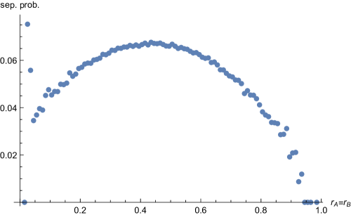
of either of the qubit subsystems ($A,B$) of $\rho$, obtained by the partial tracing over $\rho$ of the complementary subsystem–with a singularity occurring at the pure state boundary, $r_{A}=1$ (cf. Fig. 10 below). (At times below, we use the symbol $r$, to denote interchangeably, $r_{A}$ or $r_{B}$. “The Bloch sphere provides a simple representation for the state space of the most primitive quantum unit–the qubit–resulting in geometric intuitions that are invaluable in countless fundamental information-processing scenarios” Jevtic et al. (2014).)

This same $r$-invariance phenomenon appeared to hold, in general they found, for $2\times m$ [qubit-qudit] systems. (For $m>3$, the probability of having a positive partial transpose–which is now a necessary but not sufficient condition for separability–was employed (Milz and Strunz, 2015, Fig. 5).) Further, Milz indicated in a personal communication that for the $2\times 2$ qubit-qubit systems endowed with random induced measure (a function of the dimension $K$ of the ancillary space) Życzkowski and Sommers (2001); Aubrun et al. (2014), $r$-invariance of these separability probabilities–the values of which can now be directly obtained from equations (3)-(5) in Slater and Dunkl (2015b)–also seems to hold. The (symmetric) case $K=4$ is equivalent to the Hilbert-Schmidt one.

The work of Milz and Strunz is rather similar in motivation with earlier efforts in which it was sought to describe separability probabilities also as functions of single variables (but other than the Bloch radius)–namely, the “cross-product ratio” (suggested by work of Bloore Bloore (1976)), $\frac{\rho_{11}\rho_{44}}{\rho_{22}\rho_{33}}$ Slater (2007b, a, 2008), and the maximal concurrence over spectral orbits Slater (2009) (cf. Hildebrand (2007)), and the participation ratio and von Neumann-Renyi entropies (Życzkowski et al., 1998, Figs. 2b, 4) (cf. App. B below and (Khvedelidze and Rogojin, 2015, Figs. 1, 2)). None of the univariate separability functions constructed was of the highly intriguing constant form, however. (So, in a sense here, the Bloch radius serves as the extreme antithesis of an entanglement indicator, being entanglement-insensitive apparently.)

In this study, we seek to broaden the investigation of Milz and Strunz by examining the nature of the joint (bivariate) distribution of the Hilbert-Schmidt separability probability over the radii ($r_{A},r_{B}$) of both qubit subsystems of $\rho$ (sec. III) (cf. Mosseri and Dandoloff (2001); Mosseri and Ribeiro (2007)). Further, we examine the use of random induced measure for the Hilbert-Schmidt ($K=4$)-“neighboring” cases of $K=3$ and 5 (sec. IV). We will, similarly, examine the separability probability with respect to the another measure of substantial interest, the Bures Sommers and Życzkowski (2003); Bengtsson and Życzkowski (2006); Forrester and Kieburg (sec. V), concluding that–contrastingly–the Bures separability probability is not constant over $r$, but diminishes with the Bloch radius. Two-re[al]bit Caves et al. (2001); Batle et al. (2003) Hilbert-Schmidt analyses are included in sec. VI, and an apparent related “Dyson-index” effect Dumitriu and Edelman (2002) in sec. VI.1. In sec. VII, we examine how the various separability probabilities change as a function of $r$ when they are subdivided into that part arising from the determinantal inequality $|\rho^{PT}|>|\rho|$ and that from $|\rho|>|\rho^{PT}|>0$ (cf. Slater and Dunkl (2015a); Slater ). In that setting too, $r$-invariance appears to hold. Further, we attempted companion analyses for two-quater[nionic]bit systems Slater and Dunkl (2012); Fei and Joynt ; Batle et al. (2003), but encountered certain conceptual/computational issues we have yet to successfully resolve.

Appendix A develops upon the $X$-states analyses of Milz and Strunz (Milz and Strunz, 2015, Apps. A, B), finding similar results to those reported in the main body of this paper, but now also deriving certain exact formulas. In Appendix B we report some results (not directly pertaining to Bloch radii) based on an entanglement measure of Holik and Plastino (Holik and Plastino, 2011, eq. (9)).

II Background

Milz and Strunz found numerically-based evidence that the Hilbert-Schmidt volumes of the two-qubit systems and of their separable subsystems were both proportional to $(1-r_{A}^{2})^{6}$ (Milz and Strunz, 2015, eqs. (23), (30),(31)), with the consequent constant ratio of the two (simply proportional) volume functions being the aforementioned separability probability of $\frac{8}{33}$.

For the recently much-investigated “toy” model of $X$-states Mendonça et al. (2014); Yu and Eberly (2007); Ali et al. (2010) (Ellinas, 1998, App. B), occupying a seven-dimensional subspace of the full fifteen-dimensional space, it was possible for them to formally demonstrate that the counterpart volume functions, somewhat similarly, were both again proportional, but now to $(1-r_{A}^{2})^{3}$ (the square root of the higher-dimensional result). The corresponding (constant, but at $r_{A}=1$) separability probability was greater than $\frac{8}{33}$, that is $\frac{2}{5}$ (Milz and Strunz, 2015, Apps. A, B). This $\frac{2}{5}$ result was also subsequently proven in Slater and Dunkl (2015b), along with companion $X$-states findings for the broader class of random induced measures Życzkowski and Sommers (2001); Aubrun et al. (2014).

However, the joint distributions over the two radii in which we are expressly interested here in discerning (either in the $X$-states and/or full model), did not seem readily derivable, even in the analytical frameworks of those two $X$-states studies (cf. Balakrishnan and Lai (2009)). So recourse to numerical methods seemed indicated. The two marginal univariate distributions of the desired joint bivariate volume distributions should, of course, be proportional to $(1-r_{A}^{2})^{6}$ and $(1-r_{A}^{2})^{3}$ in the full and $X$-states models, respectively. (In Appendix A, we do succeed in constructing the desired bivariate $X$-states total and separable volume functions and, hence, the associated separability probability function.)

III Hilbert-Schmidt Analysis

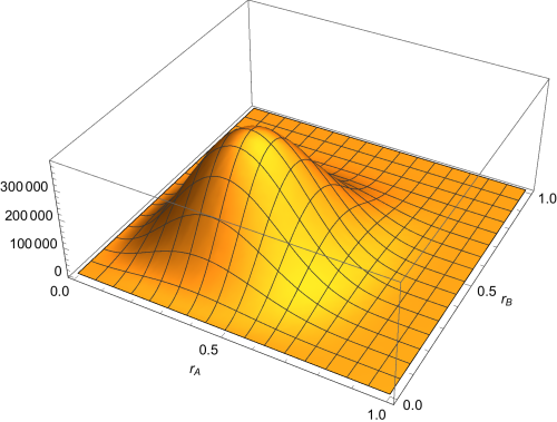
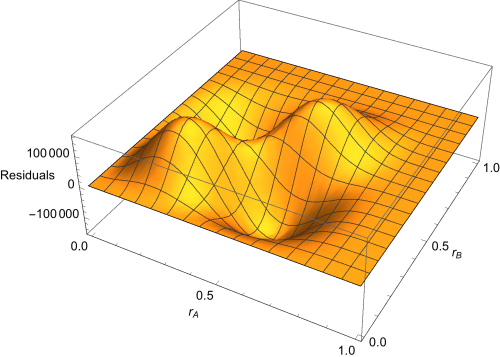
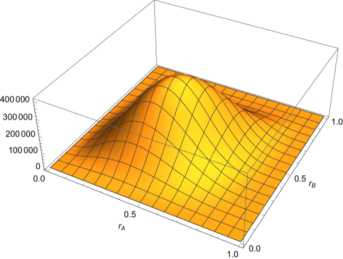
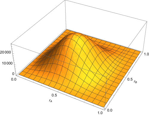
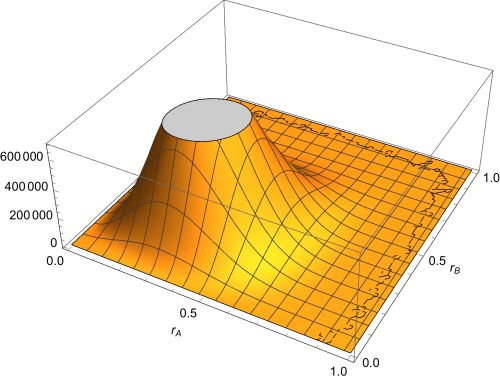
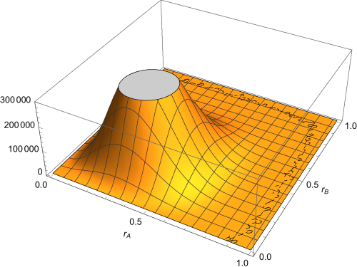
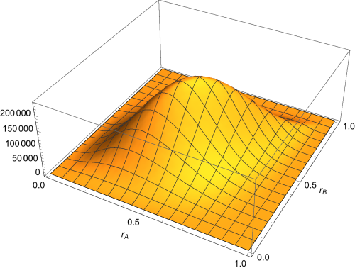
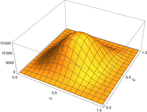
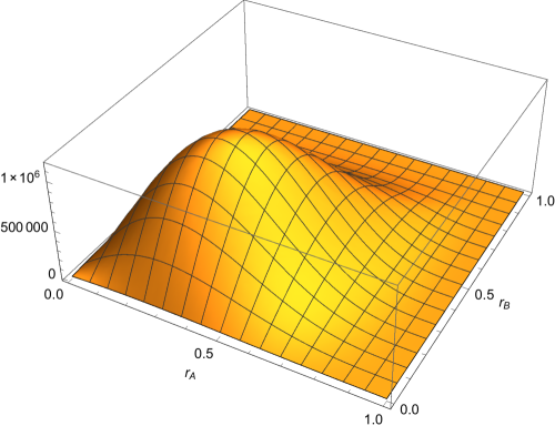
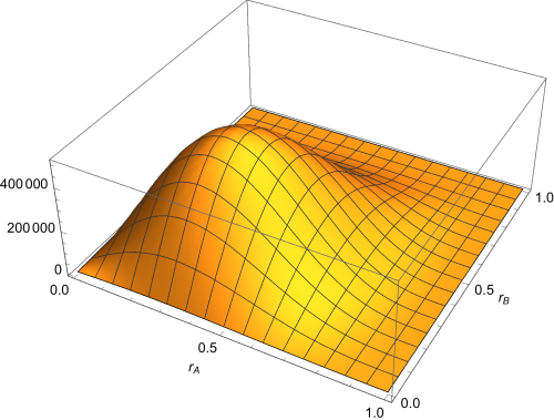
We generated 2,548,000,000 two-qubit density matrices, randomly with respect to Hilbert-Schmidt measure, using the simple (Ginibre ensemble) algorithm outlined in (Osipov et al., 2010, eq. (1)). (That is: “(a) prepare a square complex random matrix A of size N pertaining to the Ginibre ensemble (with real and imaginary parts of each element being independent normal random variables); (b) compute the matrix H = AA?/(tr AA?), (generically positive definite)” Życzkowski and Sommers (2001).) For each such matrix, we found the values of $r_{A}$ and $r_{B}$, as well as performed the well-known Peres-Horodecki (determinantal-based Demianowicz (2011)) test for separability Peres (1996); Horodecki et al. (1996) on the partial transpose of $\rho$. (That is, a two-qubit state is separable if and only if this determinant is nonnegative.) Then, we discretized/binned the values of the $r_{A}$’s and $r_{B}$’s obtained to lie in intervals of length $\frac{1}{100}$. Thus, we obtained two $100\times 100$ matrices of counts (which we symmetrize for added stability). In Figs. 1 and 2, we show the histograms of these two sets of counts (cf. (Milz and Strunz, 2015, Fig. 3)). (Of the 10,000 bins, 9,364 of the total and 9,199 of the separable ones are occupied.)

The first (total counts) plot appears to be somewhat broader in nature than the second (separable counts) plot, while appearing qualitatively rather similar.

A natural null (product/independence) hypothesis to adopt to explain the nature of Figs. 1 and 2–in light of the assertions of Milz and Strunz Milz and Strunz (2015)–is that both these surfaces are proportional (taking into account the spherical area formula) to

$$Q(r_{A},r_{B})=16\pi^{2}r_{A}^{2}r_{B}^{2}(1-r_{A}^{2})^{6}(1-r_{B}^{2})^{6}.$$ (2)

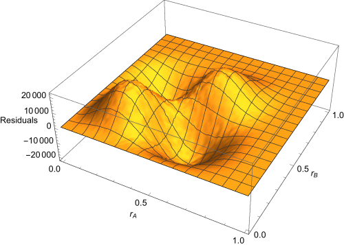
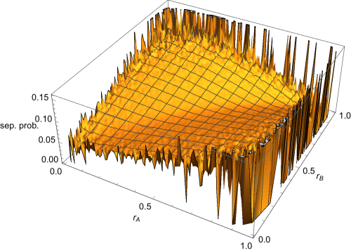
As (visual) tests of these hypotheses, we show the residuals (Figs. 3 and 4)–that is, the discrepancies (the yet unexplained amount) from the first two figures–based on such predictions. $Q(r_{A},r_{B})$ was normalized so as to minimize the sum of squares of the residuals. We note, interestingly, that both sets of residuals are bimodal in nature–as opposed to seemingly random in nature–so a null product/independence hypothesis does not seem suitable, and further analysis is required. (We can somewhat improve the fits [more so, in the total count case] by employing instead $Q(r_{A},r_{B})=16\pi^{2}r_{A}^{2}r_{B}^{2}\frac{(1-r_{A}^{2})^{8}(1-r_{B}^{2})^{8}}{(1-r_{A}^{2}r_{B}^{2})^{13}}$.)

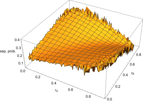
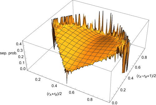
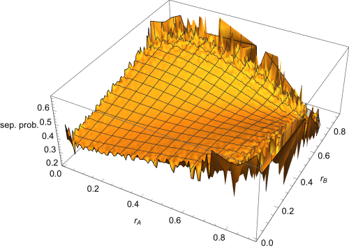
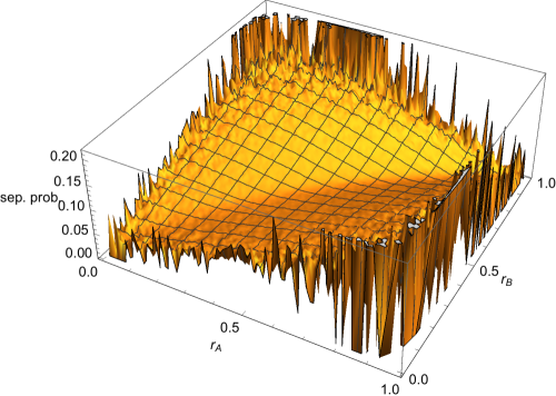
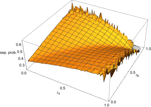
In Fig. 5, we show the estimated joint separability probabilities (the ratio of the surface in Fig. 2 to that in Fig. 1)–which are clearly now, in contrast to the univariate case–not uniform over their (unit square) domain of definition. The initial motivation for this study was to discern the functional nature of this derived (separability probability) surface.

In Fig. 6, for ease of visualization purposes, we perform a $\frac{\pi}{4}$ rotation of Fig. 5 (cf. (Braga et al., 2010, eq. (7))).

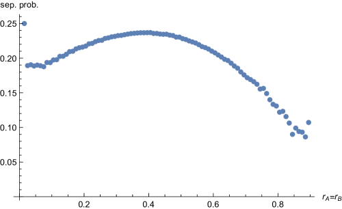
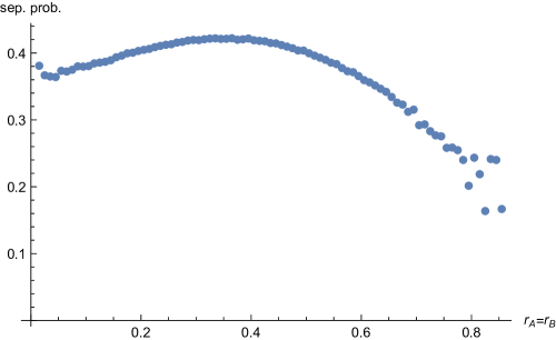
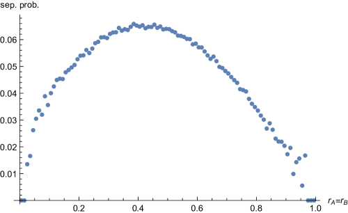
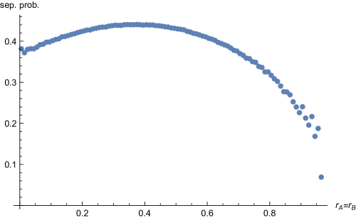
In Fig. 7 we present the $r_{A}=r_{B}$ cross-section of Fig. 5, and indicate a closely-fitting model for it. (Let us observe–certainly quite consistently with this figure–that the four Bell states are themselves unpolarized, that is $r_{A}=r_{B}=0$, and maximally entangled (cf. Mkrtchian and Chaltykyan (1987)).) For this curve, the total volume–forming the denominator of the separability probability curve–appears to be proportional to $(1-r)^{8}(1+8r)$, and the numerator comprised of the separable volume to be proportional $(1-r)^{9}(1+\frac{17}{2}r+29r^{2})$, leading to a factor of $(1-r)$ in the equation of the curve itself. The sample separability probability for those states for which $r_{A}=r_{B}$, was recorded as 0.22753675.

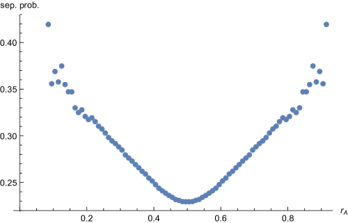
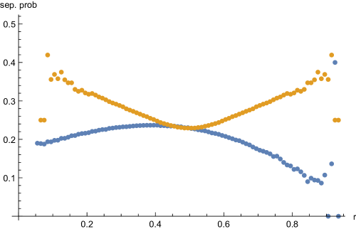
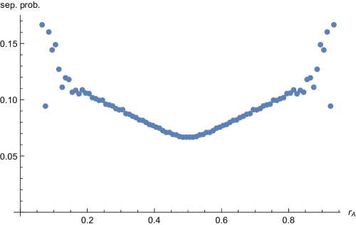
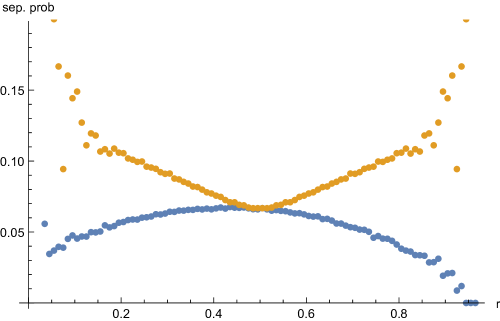
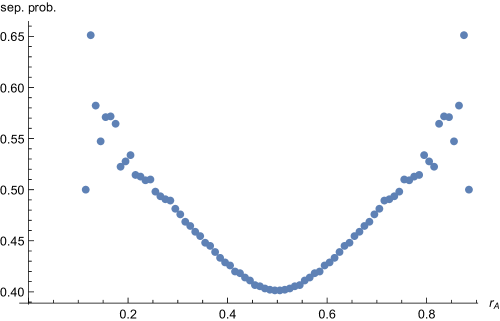
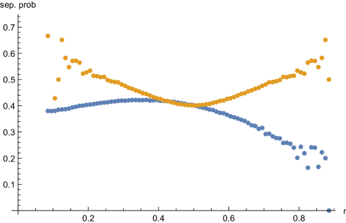
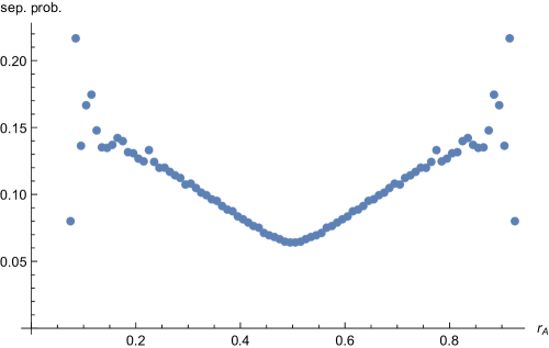
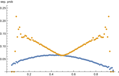
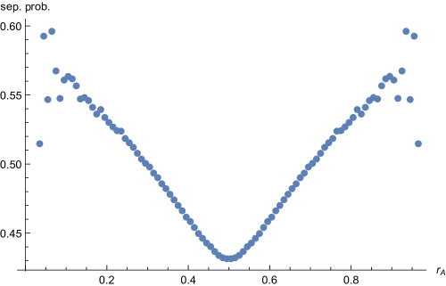
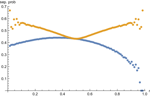
Quite contrastingly, in Fig. 8, we show the $r_{A}+r_{B}=1$ (U-shaped) cross-section of the two-dimensional separability probability surface (Fig. 5). A joint plot of these last two ($r_{A}=r_{B}$ and $r_{A}+r_{B}=1$) curves is given in Fig. 9–the first indication we have here of the titular “Bloch radii repulsion” effect.

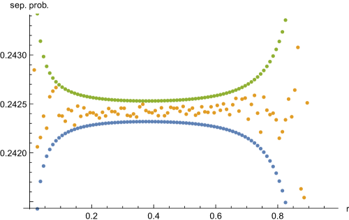
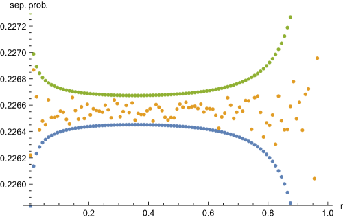
The estimated separability (marginal) probabilities over either one of the Bloch radii are shown in Fig. 10, along with a $95\%$ confidence interval (based on the suitable large-sample normal distribution approximation to the binomial distribution) about the conjectured value of $\frac{8}{33}\approx 0.242424$. (The sample estimate of this probability that we obtained here was 0.242425003.) This plot helps to confirm the chief ($r$-invariance) $2\times 2$ findings of Milz and Strunz (Milz and Strunz, 2015, Fig. 4).

IV Random Induced Measure Analyses

We explore the questions raised above, but now in the broader context of random induced measure Życzkowski and Sommers (2001); Bengtsson and Życzkowski (2006); Aubrun et al. (2014), involving the use of the natural, rotationally invariant measure on the set of all pure states of a $4\times K$ composite system (with $K=4$ yielding the Hilbert-Schmidt measure). By tracing over the $K$-dimensional ancillary system, one obtains the two-qubit states that we will analyze. We generate random matrices with respect to these measures using the algorithm specified in Miszczak (2012) (cf. Miszczak (2013)).

IV.1 The case K=3

Setting $k=K-4=-1$, in equation (2) of the recent study Slater and Dunkl (2015b),

$$P^{qubit}_{k}=1-\frac{3\ 4^{k+3}(2k(k+7)+25)\Gamma\left(k+\frac{7}{2}\right)\Gamma(2k+9)}{\sqrt{\pi}\Gamma(3k+13)},$$ (3)

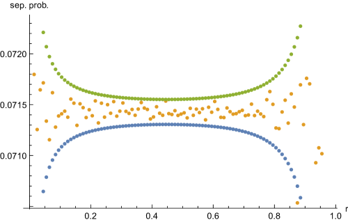
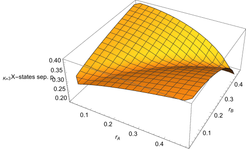
we obtain that the associated separability probability for this scenario is $\frac{1}{14}\approx 0.0714285$. The related figures–based on 764,000,000 randomly generated $4\times 4$ density matrices–are Figs. 11 to 17 (Fig. [11] total counts histogram; [12] separable counts histogram; [13] joint separability probability estimates; [14] $r_{A}=r_{B}$ curve; [15] $r_{A}+r_{B}=1$ curve; [16] joint plot of $r_{A}=r_{B}$ and $r_{A}+r_{B}=1$ curves; and [17] separability probability estimates over Bloch radius). The sample separability probability estimate is 0.0714333, quite close to the theoretically-predicted value.

For the $r_{A}=r_{B}$ curve (Fig. 14), the total volume–forming the denominator of the separability probability curve–appears to be proportional to $(1-r)^{5}$, and the numerator comprised of the separable volume to contain a factor $(1-r)^{6}$, leading–again, as in the $K=4$ case–to a factor of $(1-r)$ in the equation of the curve. The sample separability probability for those states for which $r_{A}=r_{B}$ was recorded as $\frac{3396373}{53960055}\approx 0.0629424$.

IV.2 The case K=5

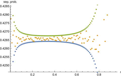
Now, inserting $k=1$ into the two-qubit random-induced formula (3) above, we obtain the associated separability probability for this scenario, $\frac{61}{143}\approx 0.426573$. The related figures–parallel to those (Figs. 11-17) for the $K=3$ analysis–are now Figs. 18 to 24 (Fig. [18] total counts histogram; [19] separable counts histogram; [20] joint separability probability estimates; [21] $r_{A}=r_{B}$ curve; [22] $r_{A}+r_{B}=1$ curve; [23] joint plot of $r_{A}=r_{B}$ and $r_{A}+r_{B}=1$ curves; and [24] separability probability estimates over Bloch radius). These are based on 1,267,000,000 randomly generated density matrices. The estimated separability probability is 0.426549.

For the $r_{A}=r_{B}$ curve (Fig. 21), the total volume–forming the denominator of the separability probability curve–appears to be proportional to $(1-r)^{11}(1+11r+40r^{2})$, and the numerator comprised of the separable volume to contain a factor $(1-r)^{12}$, leading, again, as with $K=3,4$, to an apparent factor of $(1-r)$ in the equation of the curve.

V Bures Analysis

Our analyses now are based on 424,000,000 randomly generated $4\times 4$ density matrices with respect to the Bures (minimal monotone) measure Bengtsson and Życzkowski (2006); Sommers and Życzkowski (2003), using the algorithm given in (Osipov et al., 2010, eq. (4)). Paralleling those figures given above for the $K=3$ and $K=5$ random induced measures, we present a corresponding Bures-based series of figures (Figs. 25–31) (Fig. [25] total counts histogram; [26] separable counts histogram; [27] joint separability probability estimates; [28] $r_{A}=r_{B}$ curve; [29] $r_{A}+r_{B}=1$ curve; [30] joint plot of $r_{A}=r_{B}$ and $r_{A}+r_{B}=1$ curves; and [31] separability probability estimates over Bloch radius).

Fig. 31 indicates that the separability probability in the radial direction of either reduced qubit subsystem is not constant, but diminishes with $r$, in strong contrast to the cases analyzed above. The estimate of the Bures separability probability Slater (2000, 2005); Khvedelidze and Rogojin (2015) itself that we obtain is 0.0733096. A “silver mean” conjecture for this last value, that is $\frac{1680\sigma_{Ag}}{\pi^{8}}\approx 0.0733389$, where the silver mean is defined as $\sigma_{Ag}=\sqrt{2}-1$, had been advanced in (Slater, 2005, eq. (16)). Clearly, however, the supporting case for this decade-old Bures two-qubit separability probability conjecture (based on quasi-Monte Carlo sampling, and not the more recent algorithm Osipov et al. (2010)) is not nearly as strong as is the multifaceted case that has been accumulating in the past few years for the corresponding Hilbert-Schmidt conjecture of $\frac{8}{33}$ Slater (2007a); Slater and Dunkl (2012); Slater (2013); Fei and Joynt ; Slater and Dunkl (2015a).

VI Two-Rebit Hilbert-Schmidt Analysis

We have been noting that a remarkably strong, diverse body of evidence Slater (2007a); Slater and Dunkl (2012); Slater (2013); Fei and Joynt ; Slater and Dunkl (2015a); Khvedelidze and Rogojin (2015)–though yet no formal proof (cf. Slater and Dunkl (2015b))–has been accumulating in the past several years for the proposition that the Hilbert-Schmidt separability probability of generic (15-dimensional) two-qubit states is $\frac{8}{33}\approx 0.242424$. Accompanying these results has also been evidence that the Hilbert-Schmidt separability probability of generic (9-dimensional) two-re[al]bit states Caves et al. (2001); Batle et al. (2003) is $\frac{29}{64}\approx 0.453125$.

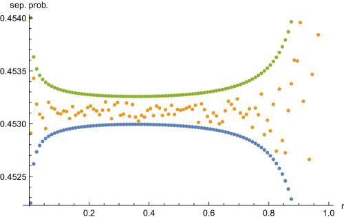
In Figs. 32-38 we present a parallel set of figures to those above, now for $4\times 4$ density matrices with real entries with respect to Hilbert-Schmidt measure (Fig. [32] total counts histogram; [33] separable counts histogram; [34] joint separability probability estimates; [35] $r_{A}=r_{B}$ curve; [36] $r_{A}+r_{B}=1$ curve; [37] joint plot of $r_{A}=r_{B}$ and $r_{A}+r_{B}=1$ curves; and [38] separability probability estimates over Bloch radius). (We follow the prescription given in (Osipov et al., 2010, p. 7) regarding the generation of such random matrices, of which we generate 2,751,000,000.) The separability probability estimate that we obtain is 0.453115. In this case, each Bloch radius has a two-dimensional, rather than a three-dimensional character (nor one-dimensional aspect, as will be the case with the $X$-states).

The two $100\times 100$ matrices of total counts in the Hilbert-Schmidt two-rebit analysis (Fig. 32) and in the Hilbert-Schmidt two-qubit analysis (Fig. 1) have 8,325 of the 10,000 cells both of size at least 100. The correlation between the estimated separability probabilities for those two sets of 8,325 cells was 0.987954. On the other hand, if we first square the values of the two-rebit separability probabilities–as random matrix (Dyson-index) theory Dumitriu and Edelman (2002) might suggest–the correlation is slightly higher, 0.989462.

VI.1 Dyson-index relations between rebit and qubit $r_{A}=r_{B}$ formulas

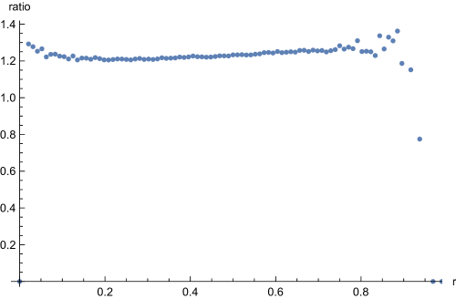
Further pursuing this Dyson-index ansatz, we plot in Fig. 39, the ratio of the estimated two-qubit $r_{A}=r_{B}$ probability distribution to the square of its two-rebit counterpart. We see that this ratio appears to hold quite constant at roughly $\frac{5}{4}$. This ratio is also, clearly, formally a ratio ($R=\frac{R_{sep}}{R_{tot}}$) of two auxiliary quantities. The numerator $R_{sep}$ is itself the ratio of the two-qubit separable volume to the square of the two-rebit separable volume, and the denominator $R_{tot}$, likewise in terms of total volumes. Our well-fitting estimates of $R_{sep}$ were $0.0023976r+0.019464$ and of $R_{tot}$, $0.0023868r+0.0171397$, respectively. So, the slopes of the two lines are extremely close, yielding–via the equivalence $\frac{R_{sep}}{R_{tot}}$–the near flatness of Fig. 39.

Along such “Dyson-index” lines of thought, we have been investigating–with some numerical encouragement–the possibility that in the $r_{A}=r_{B}$ scenarios in the two-rebit case, the volume functions might have factors of $(1-r)^{4}$ and $(1-r)^{\frac{9}{2}}$ in the total and separable cases, respectively. Such an investigation stemmed from the apparent occurrences, noted above, of factors $(1-r)^{8}$ and $(1-r)^{9}$ in the two-qubit counterpart volume functions–which appear to be, in full, proportional to $(1-r)^{8}(1+8r)$ and $(1-r)^{9}(1+\frac{17}{2}r+29r^{2})$.

We would anticipate that related Dyson-index patterns would continue to hold in the case of two-quater[nionic]bits.

VII Division of separability probabilities between $|\rho^{PT}|>|\rho|$ and $|\rho|>|\rho^{PT}|>0$

It now appears, based on the above analyses, that for the two-qubit states endowed with random induced measure, the separability probabilities are constant along either Bloch radius (except at the isolated point $r=1$) of the reduced single-qubit states (Figs. 10, 17, 24). An interesting supplementary question which we will now investigate is what are the contributions to the separability probabilities arising from the determinantal inequality $|\rho^{PT}|>|\rho|$ and, complementarily, from $|\rho|>|\rho^{PT}|>0$.

VII.1 Hilbert-Schmidt ($K=4$) case

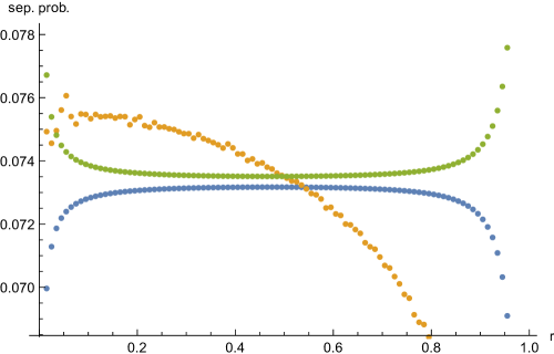
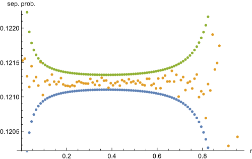
We know from preceding work (Slater and Dunkl, 2015a, Table IV) Slater that in the Hilbert-Schmidt case, the conjectured probability of $\frac{8}{33}$ appears to be evenly divided, with each inequality contributing $\frac{4}{33}$. In a further analysis conducted here, based on 1,419,000,000 random matrices, it appears that this amount of $\frac{4}{33}\approx 0.121212$ (the sample estimate being 0.121208) is–paralleling the Milz-Strunz finding for the total (undivided, that is $|\rho^{PT}|>0$) separability probability–constant along the Bloch radius of either reduced single-qubit system (Fig. 40).

VII.2 Random Induced $K=3$ case

For the $K=3$ $(k=-1)$ case, the entire separability probability of $\frac{1}{14}$ is associated with the inequality $|\rho^{PT}|>|\rho|$, so no similar nontrivial splitting can take place. (In this scenario, $\rho$ must possess at least one zero eigenvalue, and hence $|\rho|=0$, thus explaining this unique phenomenon.)

VII.3 Random Induced $K=5$ case

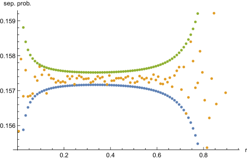
For the $K=5$ $(k=1)$ case, the total separability probability appears–as already noted (sec. IV.2)–to be $\frac{61}{143}\approx 0.426573$. Table IV of Slater and Dunkl (2015a) asserts that the proportion of this associated with $|\rho^{PT}|>|\rho|$ is $\frac{45}{122}$, yielding then $(\frac{61}{143})(\frac{45}{122})=\frac{45}{286}\approx 0.157343$. In Fig. 41, we show–based on 1,267,000,000 random matrices–an associated flat-like plot, conforming closely to this value (the overall sample estimate being 0.157323). Thus, it appears that this separability (sub-)probability–and, of course, its complementary value of $\frac{61}{143}-\frac{45}{286}=\frac{7}{26}$–is constant along either Bloch radius. So, these analyses serve as an expansion–and a type of further validation–of the Milz-Strunz findings Milz and Strunz (2015).

VII.4 Two-rebit case

In Fig. 42 we present the Hilbert-Schmidt two-rebit counterpart of these several figures, with the sample estimate of the overall separability probability of $\frac{1}{2}(\frac{29}{64})=\frac{29}{128}\approx 0.226563$, being 0.226554. (Here, the 2,751,000,000 random density matrices employed in sec. VI were again employed.)

VII.5 Bivariate Extension

Additionally, if we similarly split the three bivariate separability probability plots (Figs. 5, 20, 34) for the $K=4$, $K=5$ two-qubit and $K=4$ two-rebit cases, in accordance with the two determinantal inequalities, $|\rho^{PT}|>|\rho|$ and $|\rho|>|\rho^{PT}|>0$, the resultant plots appear alike in shape to the parent plots. So, we can certainly conjecture a similar equal splitting of probability phenomenon in that higher-dimensional domain.

VIII Concluding Remarks

All the bivariate separability probability estimates presented (Figs. 5, 13, 20, 27, 34) appear to have a saddle point at $(\frac{1}{2},\frac{1}{2})$, or somewhere in the neighborhood thereof, with the $r_{A}=r_{B}$ curves (Figs. 7, 14, 21, 28, 35), possibly achieving their maxima at $r_{A}=r_{B}=\frac{1}{2}$ and the $r_{A}+r_{B}=1$ curves (Figs. 8, 15, 22, 29, 36) attaining their minima there. A simple probability distribution over $[0,1]^{2}$ with such a saddle point property, that, in addition, has the required marginal univariate uniform distributions over $r_{A}$ or $r_{B}$, is

$$p(r_{A},r_{B})=2r_{A}+2r_{B}-4r_{A}r_{B}.$$ (4)

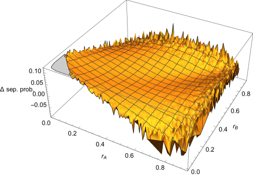
(This functional form was suggested by Brian Tung in response to a Math Stack Exchange question https://math.stackexchange.com/questions/1271549/bivariate-probability-distributions-over-unit-square-uniform-marginals-midpo.) In Fig. 43 we show the residuals/discrepancies obtained by subtracting $\frac{8p(r_{A},r_{B})}{33}$ from the estimated two-qubit Hilbert-Schmidt separability probabilities of Fig. 5.

We were able to obtain a somewhat superior fit (also satisfying the marginal constraints) to this one–as measured by the sum of absolute values of residuals from the fit–using a higher-degree form of probability distribution over the unit square, namely

$$p^{\prime}(r_{A},r_{B})=\frac{3}{2}r_{A}^{2}r_{B}+\frac{3}{2}r_{A}r_{B}^{2}-6r_{A}r_{B}-\frac{3r_{A}^{2}}{4}+\frac{5r_{A}}{2}-\frac{3r_{B}^{2}}{4}+\frac{5r_{B}}{2}.$$ (5)

From Figs. 9, 16, 23, 30 and 37 we see a form of Bloch radii repulsion. That is, separability probabilities tend to increase as the gap in value between the lengths of the two radii increase.

At this point, we have not yet achieved our motivating goal in undertaking this study, that is, to determine the precise nature of the bivariate distributions over the pair of Bloch radii.

A remaining related case that is still not successfully analyzed is that of the 27-dimensional set of generic two-quat[ernionic]bits Batle et al. (2003), for which the Hilbert-Schmidt separability probability appears to be $\frac{26}{323}\approx 0.0804954$ Slater and Dunkl (2012); Fei and Joynt . An interesting question here is how to determine the corresponding “Bloch radii” for randomly generated two-quaterbit states (cf. Brody and Graefe (2011)). Further, we have not yet developed a computationally feasible (Mathematica-implemented) algorithm for the random generation of such matrices (cf. (Dumitriu and Edelman, 2002, Fig. 1) Osipov et al. (2010); Miszczak (2012)).

Let us note that the two reduced qubit systems of a pure two-qubit system must have their Bloch radii equal (that is, totally “non-repulsive”). The separable pure two-qubit systems form a four-dimensional submanifold of the six-dimensional manifold of pure two-qubit systems (Bengtsson and Życzkowski, 2006, p. 368), and thus are of relative measure/probability zero. (These observations, it would seem, at least in an informal qualitative manner, are not inconsistent with our general set of results.) In terms of the “pseudo-pure” two-qubit states, that is those having only two distinct nondegenerate eigenvalues, Scutaru has shown that ”the Bloch vectors of the corresponding qubits are related by a rotation” Scutaru (2004).

In Table 1 we present the results of an auxiliary set of analyses. Five million random density matrices were generated for each scenario indicated, and the correlation computed between the lengths of the corresponding Bloch radii, both for all the density matrices generated, and also just for the subset of separable density matrices. The consistently smaller correlations for the separable states are a manifestation of the repulsion effect we have documented in this study. (We note, however, that none of these correlations is negative. So, perhaps rather than the term “repulsion”, the use of “relative repulsion” or “diminished attraction” might be more strictly appropriate.) Obviously, the correlations in the table based on the Bures measure are exceptionally large.

scenario	all states	separable states
Random Induced $K=5$	0.145496	0.0968024
Hilbert-Schmidt two-qubits	0.183026	0.107762
Hilbert-Schmidt two-rebits	0.176898	0.118049
Random Induced $K=3$	0.248993	0.125835
Bures two-qubits	0.388250	0.210838

Table 1: Correlations between pairs of Bloch radii for all states and all separable states for differing scenarios. The lower correlations for the separable states are consistent with a relative repulsion effect.

Evidence adduced by Milz and Strunz indicated that both the Hilbert-Schmidt total and separable univariate volume functions of two-qubit states were simply proportional to $(1-r^{2})^{6}$ (Milz and Strunz, 2015, eq. (23)). Quite supportingly, we ourselves fit a function of the form $c(1-r^{2})^{p}$ to the large sample of such states employed above (sec. III), and obtained estimates of 5.99965 and 5.99926, respectively, of this exponent for the two volumes. Similarly, for the two-rebit set of analyses (sec. VI), the estimates were 6.00439 and 6.00447. For random-induced measure with $K=3$ (sec. IV.1), 3.99973 and 4.00015 were obtained, while for the case $K=5$ (sec. IV.2), the corresponding results were 7.99923 and 7.99917. (A parallel exercise based on the Bures measure [sec. V] yielded the rather proximate–but certainly far from integral–results of 3.48845 and 3.58319, respectively.)

Following the work of Braga, Souza and Mizrahi (Braga et al., 2010, eq. (7)), it might prove advantageous in our quest to model the various bivariate total and separable volume and probability functions discussed above, to employ transformed variables of the form $u_{+}=\frac{r_{A}+r_{B}}{2}$ and $u_{-}=\frac{r_{A}-r_{B}}{2}$. In fact, this appears to be the case in the following appendix devoted to $X$-states analyses Yu and Eberly (2007); Ali et al. (2010); Ellinas (1998).

IX Appendix A: $X$-states analyses

IX.1 $X$-states bivariate formulas

We employed the $X$-states parametrization and transformations indicated by Braga, Souza and Mizrahi (Braga et al., 2010, eqs. (6), (7)). Based on these, we were formally able to reproduce the Hilbert-Schmidt univariate volume result of Milz and Strunz (Milz and Strunz, 2015, eq. (20), Fig. 1),

$$V^{(X)}_{HS}(r)=\frac{\pi^{2}}{2304}(1-r^{2})^{3},$$ (6)

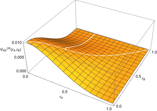
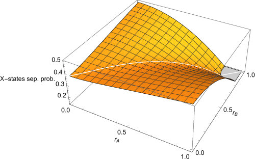
as the marginal distribution (over either $r_{A}$ or $r_{B}$) of the bivariate distribution (Fig. 44)

$$_{{tot}}V^{(X)}_{HS}(r_{A},r_{B})=$$ (7)

$$\begin{cases}-\frac{1}{960}\pi^{2}\left(r_{A}-1\right){}^{3}\left(r_{A}\left(r_{A}+3\right)-5r_{B}^{2}+1\right)&r_{A}>r_{B}\\ -\frac{1}{960}\pi^{2}\left(r_{B}-1\right){}^{3}\left(-5r_{A}^{2}+r_{B}\left(r_{B}+3\right)+1\right)&r_{A}<r_{B}.\end{cases}$$

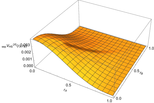
To now obtain the desired $X$-states bivariate separability probability distribution (perhaps–and hopefully–suggestive of the full 15-dimensional counterpart), we find the separable volume counterpart (Fig. 45) to (7)

$$_{{sep}}V^{(X)}_{HS}(r_{A},r_{B})=$$ (8)

$$\begin{cases}-\frac{\pi^{2}\left(r_{A}-1\right){}^{3}\left(5\left(r_{A}+3\right)r_{B}^{4}-10\left(3r_{A}+1\right)r_{B}^{2}+8r_{A}^{2}+9r_{A}+3\right)}{7680}&r_{A}>r_{B}\\ -\frac{\pi^{2}\left(r_{B}-1\right){}^{3}\left(5r_{A}^{4}\left(r_{B}+3\right)-10r_{A}^{2}\left(3r_{B}+1\right)+r_{B}\left(8r_{B}+9\right)+3\right)}{7680}&r_{A}<r_{B},\end{cases}$$

and take their ratio (Fig. 46) (noting the cancellation of the $(r-1)^{3}$-type factors), obtaining thereby the $X$-states bivariate separability probability formula,

$$p^{X-states}(r_{A},r_{B})=$$ (9)

$$\begin{cases}\frac{5\left(r_{A}+3\right)r_{B}^{4}-10\left(3r_{A}+1\right)r_{B}^{2}+8r_{A}^{2}+9r_{A}+3}{8\left(r_{A}\left(r_{A}+3\right)-5r_{B}^{2}+1\right)}&r_{A}>r_{B}\\ \frac{5r_{A}^{4}\left(r_{B}+3\right)-10r_{A}^{2}\left(3r_{B}+1\right)+r_{B}\left(8r_{B}+9\right)+3}{8\left(-5r_{A}^{2}+r_{B}\left(r_{B}+3\right)+1\right)}&r_{A}<r_{B}\end{cases}.$$

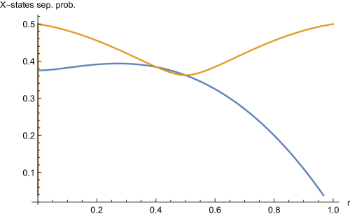
(Numerical integration of this function over $[0,1]^{2}$ yielded 0.381678.) Also, Fig. 47 shows the (lower) $r_{A}=r_{B}$ and (upper) $r_{A}+r_{B}=1$ cross-sections of Fig. 46. (We note in the next section immediately below an exception to the “repulsion” phenomenon, which we have repeatedly observed above. We computed the correlation between the pair of Bloch radii to be $1-\frac{11206656}{37748736-10080\pi^{2}+\pi^{4}}\approx 0.702341$ for all states and only slightly less, $1-\frac{74649600}{235929600-25200\pi^{2}+\pi^{4}}\approx 0.68326$, for the separable $X$-states.)

In light of the $X$-states results (7) and (8), we might speculate that the counterpart bivariate total and separable volumes for the 15-dimensional set of two-qubits states will both consist of the product of $(1-r)^{6}$ and certain polynomials. The corresponding separability probability function (cf. Fig. 5) would then be a rational one.

IX.2 Certain univariate $X$-states separability probability conditional distributions

The analytic form of the $r_{A}=r_{B}$ separability probability curve for the $X$-states is

$$p^{\{X-states\}}(r_{A}=r_{B})=-\frac{(r-1)(5r(r(r+5)+3)+3)}{32r+8}.$$ (10)

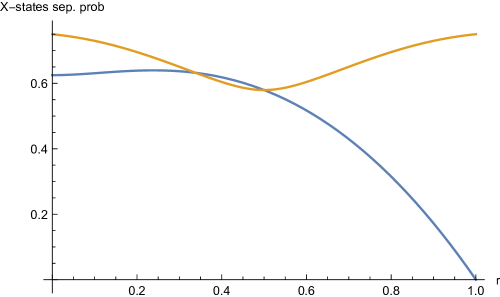
The value of this $X$-states separability probability univariate function at $(\frac{1}{2},\frac{1}{2})$ is $\frac{139}{384}=\frac{139}{2^{7}\cdot 3}$, at $(0,0)$ it is $\frac{3}{8}$, and at (1,1) it is 0. The maximum of the $r_{A}=r_{B}$ curve is achieved at the positive root ($r\approx 0.2722700792$) of the cubic equation $3r^{3}+9r^{2}+r-1=0$, its value there ($\approx 0.393558399$) being the positive root of the cubic equation $54r^{3}+108r^{2}-28r-9=0$. On the other hand, the minimum ($\frac{139}{384}\approx 0.361979$) of the $r_{A}+r_{B}=1$ curve

$$p^{\{X-states\}}(r_{A}=1-r_{B})=\begin{cases}-\frac{(r_{A}-2)r_{A}\left(5r_{A}\left(r_{A}^{2}+r_{A}-10\right)+28\right)+8}{8(r_{A}(4r_{A}-13)+4)}&2r_{A}>1\\ \frac{r_{A}(r_{A}(5r_{A}((r_{A}-4)r_{A}-6)+32)+25)-20}{8(r_{A}(4r_{A}+5)-5)}&2r_{A}<1\end{cases}$$ (11)

is attained more simply at $r_{A}=r_{B}=\frac{1}{2}$. The maximum of $\frac{1}{2}$ is situated at $r_{A}=r_{B}=0$ or 1. So, at least in this model there does not seem to be a corresponding minimax result. (Let us very interestingly note that in the interval $r\in[0.40182804,\frac{1}{2}]$, the $p^{\{X-states\}}(r_{A}=1-r_{B})$ curve is dominated by the $p^{\{X-states\}}(r_{A}=r_{B})$ curve. The maximum gap of 0.0056796160 is attained at $r=0.4564893379$. So, at least in the $X$-states setting, the ”repulsion phenomenon” does not fully hold.)

Further, setting $r_{B}=\frac{1}{2}$, we have

$$p^{\{X-states\}}(r_{B}=\frac{1}{2})=\begin{cases}\frac{r_{A}\left(128r_{A}+29\right)+23}{32\left(4r_{A}\left(r_{A}+3\right)-1\right)}&\frac{1}{2}<r_{A}<1\\ \frac{35r_{A}^{4}-50r_{A}^{2}+19}{44-80r_{A}^{2}}&0<r_{A}<\frac{1}{2}\end{cases}.$$ (12)

Putting $r_{B}=0$, we obtain

$$p^{\{X-states\}}(r_{B}=0)=\frac{r_{A}\left(8r_{A}+9\right)+3}{8\left(r_{A}\left(r_{A}+3\right)+1\right)},$$ (13)

and with $r_{B}=1$,

$$p^{\{X-states\}}(r_{B}=1)=0.$$ (14)

It certainly appears that this last result is in direct contradiction with certain assertions of Milz and Strunz: “The latter fact that $p_{sep}^{(X)}(1)=1$ is clear: a pure reduced state $(r=1)$ can only be realized by a product and thus, a separable total state” (Milz and Strunz, 2015, p. 8) (see also the discussion prior to their eq. (23)). We anticipate an eventual clarification of this apparent conflict, possibly in terms of differing dimensionalities of the measures employed.

If we restrict the $X$-states to those for which $r_{A}=r_{B}$, then the separability probability for this continuum $r_{A}\in[0,1]$ of states is $\frac{8}{21}\approx 0.3809524$. For those for which $r_{A}=1-r_{B}$, the corresponding separability probability is slightly higher, $\frac{58}{147}\approx 0.3945578$.

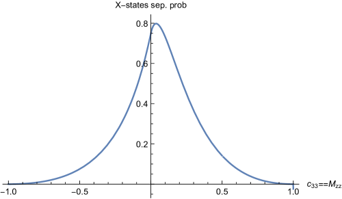
IX.3 Use of Fano correlation parameter $c_{33}=M_{zz}$

In their $X$-state studies, both Milz and Strunz Milz and Strunz (2015) and Braga, Souza and Mizrahi Braga et al. (2010) employ the well-known Fano parameterization of two-qubit systems Fano (1983). Milz and Strunz denote the Fano correlation parameter in the (conventionally denoted) $z-$ or $x_{3}$-direction by $c_{33}$, while Braga, Souza and Mizrahi employ the notation $M_{zz}$. (The alignments of the Bloch radii–$r_{A}$ and $r_{B}$–are along this same direction in the $X$-states model, we interestingly note.) Focusing on this parameter yields a number of analytic results, such as the associated $X$-states separability probability (Fig. 48). (Numerical integration of this function over [-1,1] yielded 0.416283.)

IX.4 Random Induced $K=5$ case

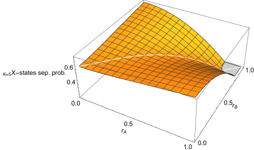
We have found here–introducing a factor of $|\rho|$ into the integrations in the previously-conducted Hilbert-Schmidt $X$-states analyses–that the total volume bivariate distribution for the induced measure case of $K=5$ equals

$$_{{tot}}V^{(X)}_{K=5}(r_{A},r_{B})=$$ (15)

$$\begin{cases}-\frac{\pi^{2}\left(r_{A}-1\right){}^{5}\left(-6r_{A}\left(r_{A}+5\right)r_{B}^{2}+r_{A}\left(r_{A}+1\right)\left(r_{A}\left(r_{A}+4\right)+5\right)+21r_{B}^{4}-6r_{B}^{2}+1\right)}{1290240}&r_{A}>r_{B}\\ -\frac{\pi^{2}\left(r_{B}-1\right){}^{5}\left(-6r_{A}^{2}\left(r_{B}\left(r_{B}+5\right)+1\right)+21r_{A}^{4}+r_{B}\left(r_{B}+1\right)\left(r_{B}\left(r_{B}+4\right)+5\right)+1\right)}{1290240}&r_{A}<r_{B}\end{cases}.$$

The total volume itself is $\frac{\pi^{2}}{9979200}\approx 9.8901759\cdot 10^{-7}$. The marginal distributions of the total volume bivariate distribution (15) are of the (again, proportional to $\pi^{2}(1-r^{2})^{n}$) form

$$V^{(X)}_{K=5}(r)=\frac{\pi^{2}(1-r^{2})^{5}}{3686400}=\frac{\pi^{2}(1-r^{2})^{5}}{2^{14}\cdot 3^{2}\cdot 5^{2}}.$$ (16)

The separable volume is given by

$$_{{sep}}V^{(X)}_{K=5}(r_{A},r_{B})=$$ (17)

$$\begin{cases}-\frac{\pi^{2}\left(r_{A}-1\right){}^{5}\left(-21\left(r_{A}+5\right)r_{B}^{6}+63\left(5r_{A}+1\right)r_{B}^{4}-27r_{A}\left(8r_{A}+5\right)r_{B}^{2}+r_{A}\left(8r_{A}\left(r_{A}+2\right)\left(r_{A}+3\right)+25\right)-27r_{B}^{2}+5\right)}{10321920}&r_{A}>r_{B}\\ -\frac{\pi^{2}\left(r_{B}-1\right){}^{5}\left(-21r_{A}^{6}\left(r_{B}+5\right)+63r_{A}^{4}\left(5r_{B}+1\right)-27r_{A}^{2}\left(r_{B}\left(8r_{B}+5\right)+1\right)+25r_{B}+8r_{B}^{2}\left(r_{B}+2\right)\left(r_{B}+3\right)+5\right)}{10321920}&r_{A}<r_{B}\end{cases}.$$

Its marginal distributions are of the form

$${}_{sep}V^{(X)}_{K=5}(r)=\frac{\pi^{2}(1-r^{2})^{5}}{5734400}=\frac{\pi^{2}(1-r^{2})^{5}}{2^{15}\cdot 5^{2}\cdot 7}.$$ (18)

The separability probability we found was $\frac{9}{14}\approx 0.642857$–a result also derivable from a formula (Dunkl and Slater, , p.13),

$$\mbox{Pr}\{|\rho^{PT}|>0\}=1-\frac{2\Gamma(2k+4)^{2}}{\Gamma(k+2)\Gamma(3k+6)},$$ (19)

inserting $k=1$. The separability probability function (Fig. 49) is

$$p^{X-states}_{K=5}(r_{A},r_{B})=$$ (20)

$$\begin{cases}\frac{-21\left(r_{A}+5\right)r_{B}^{6}+63\left(5r_{A}+1\right)r_{B}^{4}-27r_{A}\left(8r_{A}+5\right)r_{B}^{2}+r_{A}\left(8r_{A}\left(r_{A}+2\right)\left(r_{A}+3\right)+25\right)-27r_{B}^{2}+5}{8\left(-6r_{A}\left(r_{A}+5\right)r_{B}^{2}+r_{A}\left(r_{A}+1\right)\left(r_{A}\left(r_{A}+4\right)+5\right)+21r_{B}^{4}-6r_{B}^{2}+1\right)}&r_{A}>r_{B}\\ \frac{-21r_{A}^{6}\left(r_{B}+5\right)+63r_{A}^{4}\left(5r_{B}+1\right)-27r_{A}^{2}\left(r_{B}\left(8r_{B}+5\right)+1\right)+25r_{B}+8r_{B}^{2}\left(r_{B}+2\right)\left(r_{B}+3\right)+5}{8\left(-6r_{A}^{2}\left(r_{B}\left(r_{B}+5\right)+1\right)+21r_{A}^{4}+r_{B}\left(r_{B}+1\right)\left(r_{B}\left(r_{B}+4\right)+5\right)+1\right)}&r_{A}<r_{B}\end{cases}.$$

In Fig. 50, we show the $r_{A}=r_{B}$ and $r_{A}=1-r_{B}$ sections of this plot. The minimum of the $r_{A}=1-r_{B}$ section is once again found at $r=\frac{1}{2}$ with a value of $\frac{1261}{2176}=\frac{13\cdot 97}{2^{7}\cdot 17}\approx 0.579504$ there. For the $r_{A}=r_{B}$ section (cf. (10))

$$p^{X-states}_{K=5}(r_{A},r_{B})_{(r_{A}=r_{B})}=\frac{(1-r)(r(21r(r(r+8)+6)+40)+5)}{8(r(16r+7)+1)}.$$ (21)

The maximum, 0.63964, of this curve is attained at $r=0.238465$.

IX.5 Random Induced $K=6$ case

Here the total volume itself is $\frac{\pi^{2}}{9081072000}\approx 1.0868325\cdot 10^{-9}$. The marginal distributions are of the form

$$V^{(X)}_{K=6}(r)=\frac{\pi^{2}\left(1-r^{2}\right)^{7}}{2890137620}=\frac{\pi^{2}\left(1-r^{2}\right)^{7}}{2^{18}\cdot 3^{2}\cdot 5^{2}\cdot 7^{2}}.$$ (22)

The separability probability is $\frac{26}{33}$, given by (19), inserting $k=2$.

IX.6 Random Induced $K=7$ case

Here the total volume itself is $\frac{\pi^{2}}{5866372512000}\approx 1.68240328\cdot 10^{-12}$. The marginal distributions are, continuing the observed pattern, of the form

$$V^{(X)}_{K=7}(r)=\frac{\pi^{2}\left(r^{2}-1\right)^{9}}{1664719257600}=\frac{\pi^{2}\left(r^{2}-1\right)^{9}}{2^{24}\cdot 3^{4}\cdot 5^{2}\cdot 7^{2}}.$$ (23)

The separability probability is $\frac{125}{143}$, given by (19), inserting $k=3$ there.

IX.7 Random Induced $K=3$ case

The total volume is $\frac{2}{3}\pi^{2}\log^{2}(2)\approx 3.16125412$. The bivariate total volume distribution is

$${}_{{tot}}V^{(X)}_{K=3}(r_{A},r_{B})=\begin{cases}-2\pi^{2}\log^{2}(2)\left(r_{A}-1\right)&r_{A}>r_{B}\land r_{A}+r_{B}>0\land r_{A}<1\\ -2\pi^{2}\log^{2}(2)\left(r_{B}-1\right)&r_{B}>r_{A}\land r_{A}+r_{B}>0\land r_{B}<1\end{cases}$$ (24)

The two marginal distributions are of the form $\pi^{2}\left(1-r^{2}\right)\log^{2}(2)$. Here we found the separability probability to equal $\frac{1}{3}$. We have not been able to find analytic formulas for the bivariate separability volume function and the bivariate separability probability function, but in Fig. 51, we present a numerically-based estimate of the separability probability function.

X Appendix B: Separability probabilities as a function of
$||\rho-\rho^{A}\otimes\rho^{B}||_{\it{HS}}$

In a recent paper of Holik and Plastino, the expression

$$||\rho-\rho^{A}\otimes\rho^{B}||_{\it{HS}}$$ (25)

is put forth as a measure of entanglement (Holik and Plastino, 2011, eq. (9)), where $||\ldots||_{\it{HS}}$ is the Hilbert-Schmidt norm

$$||A||^{2}_{\it{HS}}=\mbox{tr}(AA^{\dagger}).$$ (26)

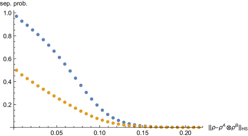
In Fig. 52 we show estimates of the two-qubit separability probabilities as a function of this term for the Hilbert-Schmidt and Bures measures, based on 54,000,000 random realizations in the former case and 43,000,000 in the latter (cf. (Khvedelidze and Rogojin, 2015, Fig. 2)). The probability diminishes as the Hilbert-Schmidt distance from product states ($\rho^{A}\otimes\rho^{B}$) increases. (Of course, it might be of some interest to employ Bures counterparts of (25) and (26)).

Figure 1: Histogram of Hilbert-Schmidt randomly sampled two-qubit density matrices parameterized by $r_{A}$ and $r_{B}$

Figure 2: Histogram of Hilbert-Schmidt randomly sampled separable two-qubit density matrices parameterized by $r_{A}$ and $r_{B}$

Figure 3: Residuals (discrepancies) from a fit to the total counts (Fig. 1) of a normalized form of $Q(r_{A},r_{B})=16\pi^{2}r_{A}^{2}r_{B}^{2}(1-r_{A}^{2})^{6}(1-r_{B}^{2})^{6}$

Figure 4: Residuals (discrepancies) from a fit to the separable counts (Fig. 2) of a normalized form of $Q(r_{A},r_{B})=16\pi^{2}r_{A}^{2}r_{B}^{2}(1-r_{A}^{2})^{6}(1-r_{B}^{2})^{6}$

Figure 5: Estimated joint Hilbert-Schmidt two-qubit separability probabilities–the ratio of the separable counts in Fig. 2 to the total counts in Fig. 1

Figure 6: $\frac{\pi}{4}$-rotation of estimated joint Hilbert-Schmidt two-qubit separability probabilities (Fig. 5)

Figure 7: Estimated Hilbert-Schmidt separability probabilities for $r_{A}=r_{B}$. A closely-fitting model (ratio of apparent separable and total volumes) for this curve is $\frac{375(1-r)\left(58r^{2}+17r+2\right)}{4096(8r+1)}$.

Figure 8: Estimated Hilbert-Schmidt two-qubit separability probabilities for $r_{A}+r_{B}=1$. A closely-fitting model for this curve is $\frac{r+4}{24r+8}$ $(0<r<\frac{1}{2})$ and $\frac{r-5}{24r-32}$ $(\frac{1}{2}<r<1)$.

Figure 9: Joint plot of the last two figures

Figure 10: Estimated (marginal) Hilbert-Schmidt two-qubit separability probabilities along either Bloch radius, together with 95$\%$ confidence limits about the conjectured value of $\frac{8}{33}\approx 0.242424$

Figure 11: Histogram of randomly sampled (with respect to the random induced $K=3$ measure) two-qubit density matrices

Figure 12: Histogram of randomly sampled (with respect to the random induced $K=3$ measure) separable two-qubit density matrices

Figure 13: Estimated joint random induced ($K=3$) separability probabilities–the ratio of Fig. 12 to Fig. 11

Figure 14: Estimated random induced ($K=3$) two-qubit separability probabilities for $r_{A}=r_{B}$. A closely-fitting model (ratio of apparent separable and total volumes) for this curve is $\frac{1}{32}(1-r)\left(r^{2}+6r+1\right)$, giving a total separability probability for the continuum of such states of $\frac{9}{143}\approx 0.0629371$. The maximum of the curve $\frac{1}{27}(5\sqrt{10}-14)\approx 0.0670885$ occurs at $r=\frac{1}{3}(2\sqrt{10}-5)\approx 0.441518$

Figure 15: Estimated random induced ($K=3$) two-qubit separability probabilities for $r_{A}+r_{B}=1$.

Figure 16: Joint plot of the last two figures

Figure 17: Estimated random induced ($K=3$) two-qubit separability probabilities over either one of the Bloch radii, along with 95$\%$ confidence limits about the conjectured value of $\frac{1}{14}\approx 0.0714285$

Figure 18: Histogram of randomly sampled (with respect to the random induced $K=5$ measure) two-qubit density matrices

Figure 19: Histogram of randomly sampled (with respect to the random induced $K=5$ measure) separable two-qubit density matrices

Figure 20: Estimated joint random induced ($K=5$) separability probabilities–the ratio of Fig. 19 to Fig. 18

Figure 21: Estimated random induced ($K=5$) two-qubit separability probabilities for $r_{A}=r_{B}$. A closely-fitting model (ratio of apparent separable and total volumes) for this curve is $\frac{(1-r)\left(\frac{87r^{3}}{2}+\frac{85r^{2}}{4}+\frac{17r}{4}+\frac{1}{3}\right)}{40r^{2}+11r+1}$.

Figure 22: Estimated random induced ($K=5$) two-qubit separability probabilities for $r_{A}+r_{B}=1$.

Figure 23: Joint plot of the last two figures

Figure 24: Estimated random induced ($K=5$) two-qubit separability probabilities over either one of the Bloch radii, along with 95$\%$ confidence limits about the conjectured value of $\frac{61}{143}\approx 0.426573$

Figure 25: Histogram of randomly sampled (with respect to the Bures measure) two-qubit density matrices

Figure 26: Histogram of randomly sampled (with respect to the Bures measure) separable two-qubit density matrices

Figure 27: Estimated joint Bures two-qubit separability probabilities–the ratio of Fig. 26 to Fig. 25

Figure 28: Estimated Bures two-qubit separability probabilities for $r_{A}=r_{B}$

Figure 29: Estimated Bures two-qubit separability probabilities for $r_{A}+r_{B}=1$

Figure 30: Joint plot of the last two figures

Figure 31: Estimated Bures two-qubit separability probabilities over either one of the Bloch radii, along with ill-fitting (in contrast to Hilbert-Schmidt and random induced) 95$\%$ confidence limits about the conjectured overall probability of $\frac{1680(\sqrt{2}-1)}{\pi^{8}}\approx 0.0733389$.

Figure 32: Histogram of randomly sampled two-rebit density matrices

Figure 33: Histogram of randomly sampled separable two-rebit density matrices

Figure 34: Estimated joint Hilbert-Schmidt two-rebit separability probabilities–the ratio of Fig. 33 to Fig. 32

Figure 35: Estimated Hilbert-Schmidt two-rebit separability probabilities for $r_{A}=r_{B}$

Figure 36: Estimated Hilbert-Schmidt two-rebit separability probabilities for $r_{A}+r_{B}=1$

Figure 37: Joint plot of the last two figures

Figure 38: Estimated (marginal) Hilbert-Schmidt two-rebit separability probabilities over either one of the Bloch radii, along with 95$\%$ confidence limits about the conjectured value of $\frac{29}{64}\approx 0.4531250$

Figure 39: Ratio of the separability probability $p^{2-qubit}(r_{A}=r_{B})$ to the square of the separability probability $p^{2-rebit}(r_{A}=r_{B})$

Figure 40: Estimated two-qubit separability probability for the Hilbert-Schmidt case $(k=0)$ associated with the determinantal inequality $|\rho^{PT}|>|\rho|$, along with 95$\%$ confidence limits about $\frac{1}{2}(\frac{8}{33})=\frac{4}{33}\approx 0.121212$.

Figure 41: Two-qubit separability probability for the random induced measure case of $K=5$ $(k=1)$ associated with the inequality $|\rho^{PT}|>|\rho|$, along with 95$\%$ confidence limits about $\frac{45}{286}\approx 0.157343$, with the complementary probability for $|\rho|>|\rho^{PT}|>0$ being $\frac{61}{143}-\frac{45}{286}=\frac{7}{26}\approx 0.269231$.

Figure 42: Two-rebit separability probability for the Hilbert-Schmidt case associated with the inequality $|\rho^{PT}|>|\rho|$, along with 95$\%$ confidence limits about $(\frac{1}{2})(\frac{29}{64})=\frac{29}{128}\approx 0.2265625$.

Figure 43: Residuals (discrepancies) of fit of $\frac{8p(r_{A},r_{B})}{33}$–given by (4)–to the estimated Hilbert-Schmidt two-qubit separability probabilities given in Fig. 5.

Figure 44: Bivariate Hilbert-Schmidt volume distribution (7) for the $X$-state model

Figure 45: Bivariate Hilbert-Schmidt separable volume distribution (8) for the $X$-state model

Figure 46: Bivariate Hilbert-Schmidt separability probability distribution (9) for the $X$-state model–the ratio of Fig. 45 to Fig. 44

Figure 47: (Lower) $r_{A}=r_{B}$–given by (10)–and (upper) $r_{A}+r_{B}=1$ curves–given by (11)–for bivariate Hilbert-Schmidt $X$-states separability probability distribution. The minimum of the upper curve is at $r=\frac{1}{2}$, while the maximum of the lower curve is at 0.27227007. In the interval $r\in[0.40182804,\frac{1}{2}]$ the $p^{\{X-states\}}(r_{A}=1-r_{B})$ curve is dominated by the $p^{\{X-states\}}(r_{A}=r_{B})$ curve.

Figure 48: $X$-states separability probability as a function of the Fano correlation parameter $c_{33}\equiv M_{zz}$. For $-1<M_{zz}<0$, the curve is simply $\frac{3\left(M_{\text{zz}}+1\right){}^{2}}{2\left(M_{\text{zz}}-2\right)\left(2M_{\text{zz}}-1\right)}.$ The maximum ($\approx 0.79819147$) occurs near $c_{33}\equiv M_{zz}=0.03677089.$

Figure 49: Bivariate separability probability function (eq. (20)) for the $K=5$ induced measure $X$-states model

Figure 50: The $r_{A}=r_{B}$ and (largely dominant) $r_{A}=1-r_{B}$ sections of the $K=5$ $X$-states separability probability function (20)

Figure 51: Numerically-based estimate of bivariate separability probability function for the $K=3$ induced measure $X$-states model

Figure 52: Two-qubit separability probabilities as a function of the entanglement expression $||\rho-\rho^{A}\otimes\rho^{B}||_{\it{HS}}$ for the Hilbert-Schmidt (dominant curve) and Bures measures

References

- Slater (2007a) P. B. Slater, J. Phys. A 40, 14279 (2007a).
- Slater and Dunkl (2012) P. B. Slater and C. F. Dunkl, J. Phys. A 45, 095305 (2012).
- Slater (2013) P. B. Slater, J. Phys. A 46, 445302 (2013).
- (4) J. Fei and R. Joynt, eprint arXiv.1409:1993.
- Slater and Dunkl (2015a) P. B. Slater and C. F. Dunkl, J. Geom. Phys. 90, 42 (2015a).
- Khvedelidze and Rogojin (2015) A. Khvedelidze and I. Rogojin, Zap. Nauchn. Sem. POMI 432, 274 (2015).
- Fonseca-Romero et al. (2012) K. M. Fonseca-Romero, J. M. Martinez-Rincón, and C. Viviescas, Phys. Rev. A 86, 042325 (2012).
- Shang et al. (2015) J. Shang, Y.-L. Seah, H. K.Ng, D. J. Nott, and B.-T. Englert, New J. Phys. 17, 043017 (2015).
- Życzkowski and Sommers (2003) K. Życzkowski and H.-J. Sommers, J. Phys. A 36, 10115 (2003).
- Bengtsson and Życzkowski (2006) I. Bengtsson and K. Życzkowski, Geometry of Quantum States (Cambridge, Cambridge, 2006).
- Milz and Strunz (2015) S. Milz and W. T. Strunz, J. Phys. A 48, 035306 (2015).
- Jevtic et al. (2014) S. Jevtic, M. Pusey, D. Jennings, and T. Rudolph, Phys. Rev. Lett. 113, 020402 (2014).
- Życzkowski and Sommers (2001) K. Życzkowski and H.-J. Sommers, J. Phys. A A34, 7111 (2001).
- Aubrun et al. (2014) G. Aubrun, S. J. Szarek, and D. Ye, Commun. Pure Appl. Math. LXVII, 0129 (2014).
- Slater and Dunkl (2015b) P. B. Slater and C. F. Dunkl, Adv. Math. Phys. 2015, 621353 (2015b).
- Bloore (1976) F. J. Bloore, J. Phys. A 9, 2059 (1976).
- Slater (2007b) P. B. Slater, Phys. Rev. A 75, 032326 (2007b).
- Slater (2008) P. B. Slater, J. Geom. Phys. 58, 1101 (2008).
- Slater (2009) P. B. Slater, J. Phys. A 42, 465305 (2009).
- Hildebrand (2007) R. Hildebrand, J. Math. Phys. 48, 102108 (2007).
- Życzkowski et al. (1998) K. Życzkowski, P. Horodecki, A. Sanpera, and M. Lewenstein, Phys. Rev. A 58, 883 (1998).
- Mosseri and Dandoloff (2001) R. Mosseri and R. Dandoloff, J. Phys. A 34, 10243 (2001).
- Mosseri and Ribeiro (2007) R. Mosseri and P. Ribeiro, Math. Structures in Comp. Sci. 17, 1117 (2007).
- Sommers and Życzkowski (2003) H.-J. Sommers and K. Życzkowski, J. Phys. A 36, 10083 (2003).
- (25) P. J. Forrester and M. Kieburg, eprint arXiv:1410.6883.
- Caves et al. (2001) C. M. Caves, C. A. Fuchs, and P. Rungta, Found. Phys. Letts. 14, 199 (2001).
- Batle et al. (2003) J. Batle, A. R. Plastino, M. Casas, and A. Plastino, Opt. Spect. 94, 759 (2003).
- Dumitriu and Edelman (2002) I. Dumitriu and A. Edelman, J. Math. Phys. 43, 5830 (2002).
- (29) P. B. Slater, eprint arXiv:1504.04555.
- Holik and Plastino (2011) F. Holik and A. Plastino, Phys. Rev. A 84, 062327 (2011).
- Mendonça et al. (2014) P. Mendonça, M. A. Marchiolli, and D. Galetti, Anns. Phys. 351, 79 (2014).
- Yu and Eberly (2007) T. Yu and J. H. Eberly, Quant. Inform. Comput. 7, 459 (2007).
- Ali et al. (2010) M. Ali, A. R. P. Rau, and G. Abler, Phys. Rev. A 81, 042105 (2010).
- Ellinas (1998) D. Ellinas, in Proc. Fourth Workshop on Physics and Computation (PhysComp96), edited by T. Toffoli and M. Biafore (New England Complex Systems Institute, Boston, 1998), chap. 10, pp. 108–109.
- Balakrishnan and Lai (2009) N. Balakrishnan and C. Lai, Continuous Bivariate Distributions (Springer, New York, 2009).
- Osipov et al. (2010) V. A. Osipov, H.-J. Sommers, and K. Życzkowski, J. Phys. A 43, 055302 (2010).
- Demianowicz (2011) M. Demianowicz, Phys. Rev. A 83, 034301 (2011).
- Peres (1996) A. Peres, Phys. Rev. Lett. 77, 1413 (1996).
- Horodecki et al. (1996) M. Horodecki, P. Horodecki, and R. Horodecki, Phys. Lett. A 223, 1 (1996).
- Braga et al. (2010) H. Braga, S. Souza, and S. S. Mizrahi, Phys. Rev. A 81, 042310 (2010).
- Mkrtchian and Chaltykyan (1987) V. E. Mkrtchian and V. O. Chaltykyan, Opt. Commun. 63, 239 (1987).
- Miszczak (2012) J. A. Miszczak, Comput. Phys. Commun. 183, 118 (2012).
- Miszczak (2013) J. A. Miszczak, Comput. Phys. Commun. 184, 257 (2013).
- Slater (2000) P. B. Slater, Euro. Phys. J. B 17, 471 (2000).
- Slater (2005) P. B. Slater, J. Geom. Phys. 53, 74 (2005).
- Brody and Graefe (2011) D. C. Brody and E.-M. Graefe, Phys. Rev. D 84, 125016 (2011).
- Scutaru (2004) H. Scutaru, Proc. Romanian Acad., Ser. A 5, 1 (2004).
- Fano (1983) U. Fano, Rev. Mod. Phys. 55, 855 (1983).
- (49) C. F. Dunkl and P. B. Slater, eprint arXiv:1501.02289 (to appear in Random Matrices: Theory and Applications).
Acknowledgements.
I would like to express appreciation to Simon Milz and Charles Dunkl–who suggested the use of confidence bands–for helpful communications.