Optical Hall conductivity of a Floquet Topological Insulator

Abstract

Results are presented for the optical Hall conductivity of a Floquet topological insulator (FTI) for an ideal closed quantum system, as well as an open system in a nonequilibrium steady-state with a reservoir. The steady-state, even for the open system, is strongly dependent on the topological phase of the FTI, with certain phases showing a remarkable near-cancellation from pockets of Berry-curvature of opposite signs, leading to a suppressed low-frequency Hall conductivity, that also shows an anomalous temperature dependence, by increasing as the temperature of the reservoir is increased. Such a behavior is in complete contrast to heating, and arises because of a strong modification of the effective system-reservoir coupling by the laser. The Berry curvature of the Floquet modes is time-dependent, and its frequency components are found to control the main features of the high-frequency Hall conductivity.

I Introduction

Topological systems are characterized by a bulk-edge correspondence where geometric properties of the bulk band-structure have a precise connection with the nature of excitations at the edge when the system is placed in a confined geometry. For an integer quantum Hall system for example, bulk bands have a non-zero Chern number $C$, which also equals the number of chiral edge modes Thouless et al. (1982); Bellissard et al. (1994); Avron et al. (1994). This correspondence implies that many bulk measurements are indirect probes of edge excitations as well. For example, the dc Hall conductivity at zero temperature, (which is equal to the Hall conductance measured in a multi-terminal measurement Klitzing et al. (1980)) is universal $\sigma_{xy}^{\rm dc}=\sigma_{xy}(\omega=0)=Ce^{2}/h$, and proportional to the number of edge-states. Moreover, the optical Hall conductivity $\sigma_{xy}\left(\omega\neq 0\right)$, while non-universal, nevertheless shows signatures of quantum Hall plateaus as the external magnetic field is varied Morimoto et al. (2009). In fact an all optical measurement such as Faraday rotation $\Theta_{F}$ of linearly polarized light of frequency $\omega$ is related to the optical Hall conductivity as $\Theta_{F}\left(\omega\right)\sim\alpha c_{n}\sigma_{xy}(\omega)$ [$\alpha$ being the fine-structure constant, and $c_{n}$ being a material dependent parameter such as the refractive index] O’Connell and Wallace (1982), and has been used as an alternate probe of quantum Hall physics, both in semiconductor heterostructures Ikebe et al. (2010), and graphene Crassee et al. (2011); Shimano et al. (2013).

Chern insulators are topological insulators (TIs) which show quantum Hall physics in the absence of a magnetic field, where time-reversal symmetry is broken by introducing complex hopping amplitudes Haldane (1988). This can be achieved by the application of a circularly polarized laser Oka and Aoki (2009); Inoue and Tanaka (2010); Kitagawa et al. (2010); Lindner et al. (2011); Gu et al. (2011); Katan and Podolsky (2013), where TIs arising out of such time-periodic perturbations are referred to as Floquet TIs (FTIs) Lindner et al. (2011). The field of FTIs has grown in recent years because of several experimental realizations ranging from periodically shaken lattices of cold-atomic gases Jotzu et al. (shed), to graphene Karch et al. (2010, 2011) and Dirac fermions on the surface of 3D TIs Wang et al. (2013) under external irradiation, and also arrays of twisted photonic waveguides Rechstman et al. (2013). In fact FTIs are extremely rich, showing different topological phases as the amplitude, frequency, and polarization of the periodic drive is varied Rudner et al. (2013); Kundu et al. (2014); Carpentier et al. (2015); Dehghani et al. (2015).

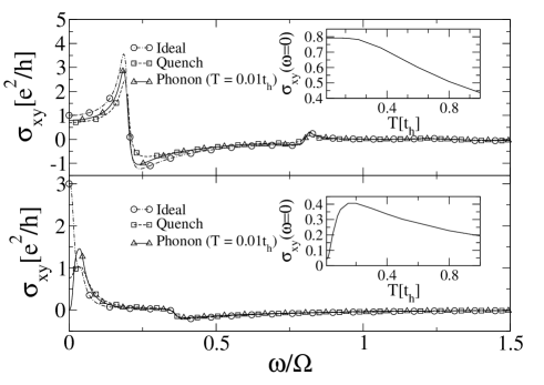
Figure 1: Optical Hall conductivity (main panel) with temperature dependence of the dc Hall conductivity (inset) for laser frequency $\Omega=5.0t_{h}$. The laser amplitude and Chern number are upper-panel: $A_{0}a=1.5,C=1$, lower-panel: $A_{0}a=0.5,C=3$ .

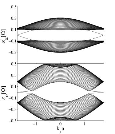
Figure 2: Quasi-energies in a cylindrical geometry highlighting edge states. The laser frequency is $\Omega=5.0t_{h}$, while the laser amplitude and Chern number are (upper panel) $A_{0}a=1.5,C=1$ and (lower panel) $A_{0}a=0.5,C=3$. The latter shows edge-states both at the center and the edges of the FBZ.

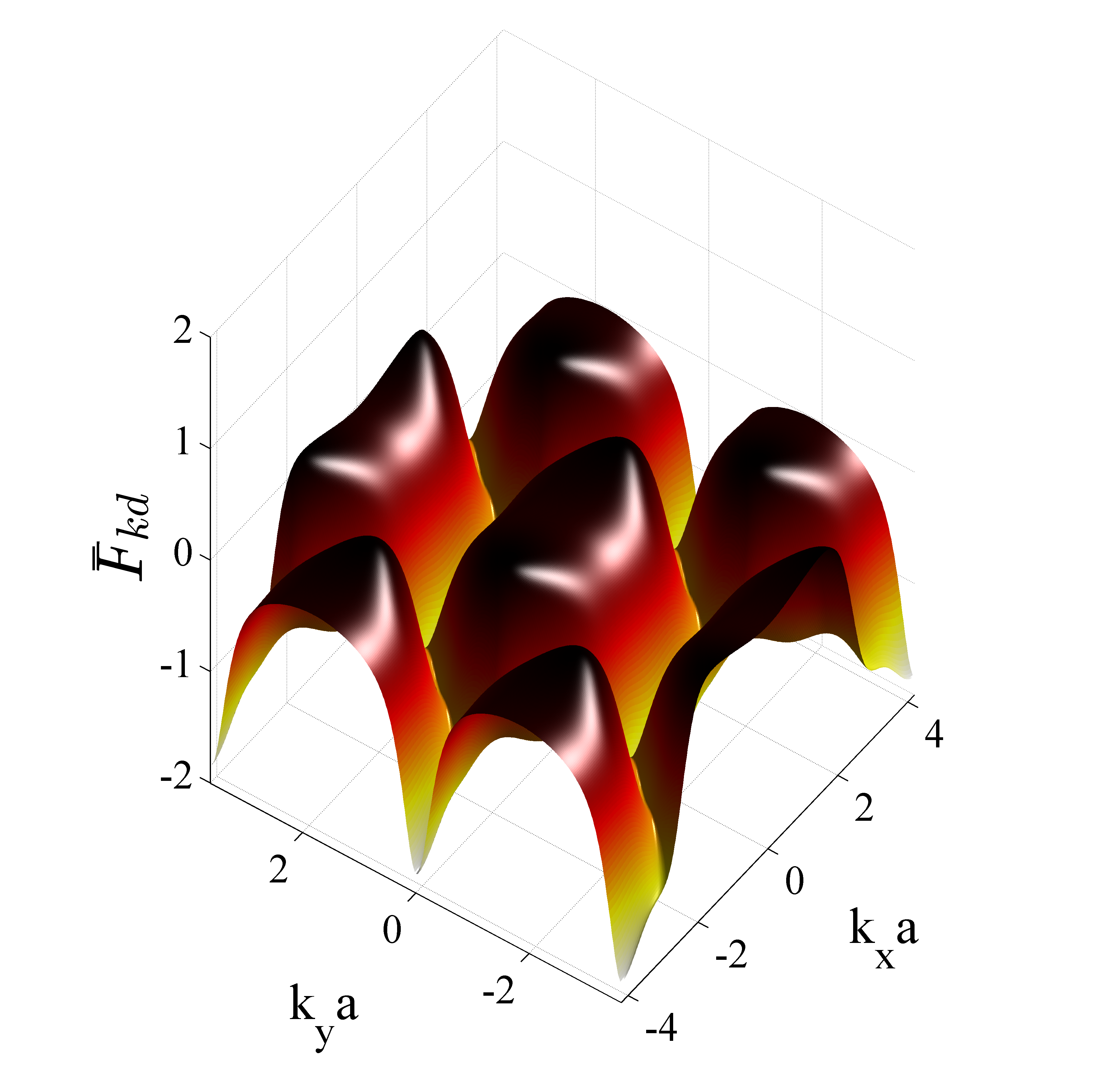
Figure 3: (color online) Time-averaged Berry curvature over 4 BZs for $\Omega=5t_{h},A_{0}a=1.5$ corresponding to a Chern number of $C=1$. The structure is rather smooth, moreover in the Fourier decomposition of $F_{kd}(t)$, two harmonics ($F_{k}^{m=0,1}$) are dominant.

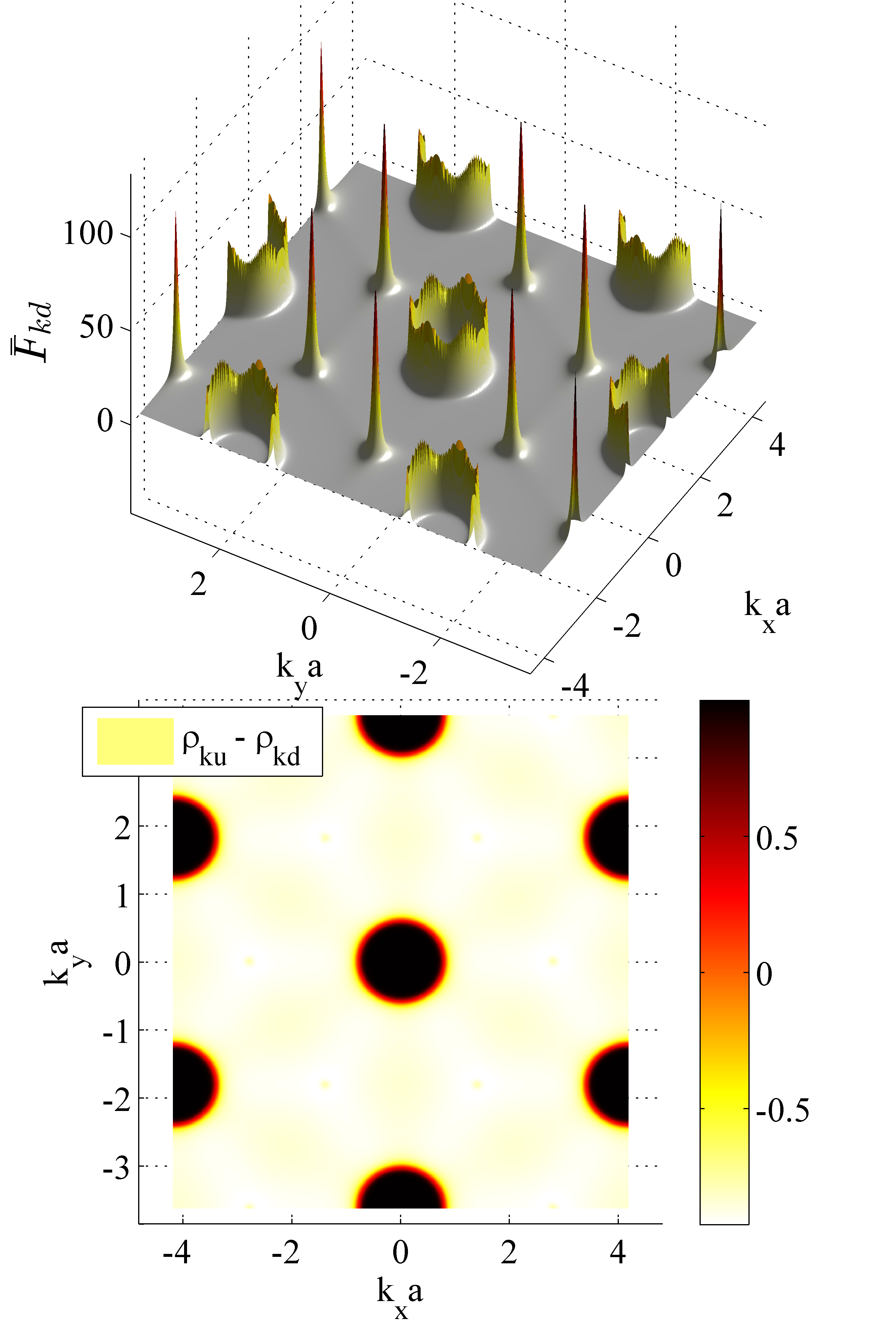
Figure 4: (color online) Upper panel: Time-averaged Berry curvature over 4 BZs for $\Omega=5.0t_{h},A_{0}a=0.5,C=3$. Lower panel: Contour plot for the steady-state population difference for reservoir temperature $T=0.01t_{h}$. Note the almost complete population inversion between regions around the Dirac points and the circles.

In this work we present results for the optical Hall conductivity of FTIs by accounting for the fact that these systems are far out of equilibrium. To this end, the precise relaxation mechanisms need to be specified as they sensitively affect results. Thus we present results for two rather different cases, one where the system is closed and the laser is switched on as a quench, while the second is when the system is coupled to an ideal reservoir, and so the steady-state loses memory of its initial state. Yet being a driven dissipative system, the steady-state is far from thermal, resulting in some unusual behavior for the Hall conductivity, which is sensitive to the topological phase, and cannot be interpreted as simply “heating”. In fact we show that the laser parameters, and in particular the topological phase, strongly affects the effective system-reservoir coupling, and therefore the steady-state, and its Hall response.

The advantage of the optical Hall conductivity is that it can be measured both in traditional multi-terminal measurements Datta (1997); Torres et al. (2014); Farrell and Pereg-Barnea (shed), as well as completely optically via the Faraday rotation, the latter being more suitable for present day experiments. In fact even the dc limit can be studied without leads, in optical lattices, by monitoring the transverse drift in time-of-flight measurements Jotzu et al. (shed). Moreover while it is the dc ($\omega\rightarrow 0$) limit of the Hall conductivity, combined with an ideal electron distribution function, that is related to a topological quantity, namely the Chern number of the Floquet bands Oka and Aoki (2011); Dehghani et al. (2015), we show that even at non-zero frequencies, some features of the topological nature of the system survive. In particular, the Berry-curvature of Floquet bands is time-dependent, and we show that various frequency components of this Berry-curvature can be directly probed in the optical Hall conductivity.

The paper is organized as follows. The model is introduced in Section II and the derivation of the Floquet-Master equation for the open system is outlined (with some details relegated to Appendix A). In Section III the optical Hall conductivity is derived using a linear-response approach, while in Section IV results for the optical Hall conductivity are presented. Finally in Section V we present our conclusions.

II Model

Our model is graphene irradiated by a circularly polarized laser, and also coupled to a phonon bath. The Hamiltonian is, $H=H_{\rm el}+H_{\rm ph}+H_{c}$ where (setting $\hbar=1$) $H_{\rm el}$ is the electronic part,

$$H_{\rm el}\!\!=-t_{h}\sum_{k}\begin{pmatrix}c_{kA}^{\dagger}&c_{kB}^{\dagger}\end{pmatrix}\!\!\begin{pmatrix}0&h_{k}^{AB}(t)\\ \left[h_{k}^{AB}(t)\right]^{*}&0\end{pmatrix}\!\!\begin{pmatrix}c_{kA}\\ c_{kB}\end{pmatrix}$$ (1)

where $h^{AB}_{k}(t)=\sum_{i=1,2,3}e^{ia(\vec{k}+\vec{A}(t))\cdot\vec{\delta}_{i}}$, $\vec{\delta}_{i}$ are the nearest-neighbor unit-vectors of graphene, $a$ is the lattice spacing, and $\vec{A}$ is the circularly polarized laser of amplitude $A_{0}$ and frequency $\Omega$, $A_{x}(t)=\theta(t)A_{0}\cos\Omega t;A_{y}(t)=-\theta(t)A_{0}\sin\Omega t$, which we assume has been suddenly switched on at time $t=0$. We consider dissipation arising due to 2D phonons $H_{\rm ph}=\sum_{q,i=x,y}\left[\omega_{qi}b_{qi}^{\dagger}b_{qi}\right]$ which are coupled to the electrons as

$$H_{c}=\sum_{{k}q\sigma,\sigma^{\prime}=A,B}c_{k+q\sigma}^{\dagger}\vec{M}_{\rm el-ph}(k,q)\cdot\vec{\sigma}_{\sigma\sigma^{\prime}}c_{{k}\sigma^{\prime}}$$ (2)

$\sigma$ is a pseudospin label denoting the $A,B$ sub-lattices, and the electron-phonon coupling $\vec{M}_{\rm el-ph}(k,q)=\left[\lambda_{x,kq}\left(b_{x,-q}^{\dagger}+b_{x,q}\right),\lambda_{y,kq}\left(b_{y,-q}^{\dagger}+b_{y,q}\right)\right]$ is off-diagonal in pseudo-spin space Suzuura and Ando (2002); Ando (2006). While we will consider only inter-(quasi)-energy-band transitions driven by long-wavelength optical phonons, our result showing that the effective matrix-elements of the electron-phonon coupling is modified by the laser, leading to nonequilibrium steady-states that depend strongly on the topological phase of the FTI, is rather general, and will carry over to other kinds of system-reservoir couplings.

We assume that initially the system is in the ground state of graphene $|\Psi(t=0)\rangle=\prod_{k}|\psi_{\rm in,k}\rangle$, and we time-evolve the system according to $H$. For the closed system ($H_{c}=0$), this time-evolution can be studied exactly, while in the presence of phonons, we solve the problem by assuming a weak electron-phonon coupling, and a very fast bath so that a Floquet-Markov approximation can be made Kohler et al. (2005); Kohn (2001); Hone et al. (2009); Dehghani et al. (2014, 2015); Suppmat.

Let us denote $W(t)$ to be the full density matrix obeying $dW(t)/dt=-i\left[H,W(t)\right]$, which in the interaction representation becomes, $W_{I}(t)=e^{iH_{\rm ph}t}U^{\dagger}_{\rm el}(t,0)W(t)U_{\rm el}(t,0)e^{-iH_{\rm ph}t}$, where $U_{\rm el}(t,t^{\prime})=\prod_{k}U_{k}(t,t^{\prime})$ is the time-evolution operator for the electrons under a periodic drive, and $U_{k}(t,t_{0})=\sum_{\alpha=u,d}e^{-i\epsilon_{k\alpha}(t-t_{0})}|\phi_{k\alpha}(t)\rangle\langle\phi_{k\alpha}(t_{0})|$ with $|\phi_{k\alpha}(t)\rangle,\epsilon_{k\alpha}$ being the quasi-modes and quasi-energies that obey $\biggl{[}H_{\rm el}-i\partial_{t}\biggr{]}|\phi_{k\alpha}\rangle=\epsilon_{k\alpha}|\phi_{k\alpha}\rangle$. We restrict the quasi-energies to a Floquet Brillouin zone (FBZ), $-\Omega/2<\epsilon_{k\alpha}<\Omega/2$, where the two quasi-energy levels are labeled $\epsilon_{ku}>\epsilon_{kd}$. The electron reduced density matrix, obtained from tracing over the phonons, $W^{\rm el}={\rm Tr}_{\rm ph}W$, has the following form in the interaction representation, $W^{\rm el}_{I}(t)=\prod_{k}\sum_{\alpha\beta}\rho_{k,\alpha\beta}(t)|\phi_{k\alpha}(t)\rangle\langle\phi_{k\beta}(t)|$. For a quench switch-on, the physically relevant initial condition is given by the overlap between the initial state and the Floquet modes at $t=0$, $\rho_{k,\alpha\beta}(t=0)=\rho_{k,\alpha\beta}^{\rm quench}=\langle\phi_{k\alpha}(0)|\psi_{{\rm in},k}\rangle\langle\psi_{{\rm in},k}|\phi_{k\beta}(0)\rangle$. Under assumptions that the bath is Markovian, always stays in thermal equilibrium at temperature $T$, and that the electron-reservoir coupling is small in comparison to all quasi-energy level spacings Hone et al. (2009), the density matrix obeys the equation of motion, $\dot{\rho}_{k,\alpha\alpha}(t)=-\sum_{\beta=u,d}L^{k}_{\alpha\alpha;\beta\beta}\rho_{k,\beta\beta}(t)$, where $L^{k}_{\alpha\alpha,\beta\beta}$ are the scattering rates. The steady-state solution is:

$$\rho_{k,\alpha\alpha}(t=\infty)=\rho_{k\alpha}$$ (3)

$$\rho_{ku}=\frac{|L^{k}_{uu,dd}|}{\biggl{(}|L^{k}_{uu,dd}|+|L^{k}_{uu,uu}|\biggr{)}},\rho_{kd}=1-\rho_{ku}$$ (4)

where the scattering rates for a constant electron-phonon coupling ($\lambda_{x,qk}=\lambda_{y,qk}=\lambda$) with a broad phonon density of states $D_{\rm ph}$ are,

$$L^{k}_{uu,uu}=\sum_{n=\rm int}M^{n}_{k}\biggl{[}\theta(-\epsilon_{kd}+\epsilon_{ku}+n\Omega)\bar{N}(-\epsilon_{kd}+\epsilon_{ku}+n\Omega)+\theta(\epsilon_{kd}-\epsilon_{ku}-n\Omega)N(\epsilon_{kd}-\epsilon_{ku}-n\Omega)\biggr{]}$$ (5)

$$-L^{k}_{uu,dd}=\sum_{n=\rm int}M_{k}^{n}\biggl{[}\theta(\epsilon_{kd}-\epsilon_{ku}-n\Omega)\bar{N}(\epsilon_{kd}-\epsilon_{ku}-n\Omega)+\theta(-\epsilon_{kd}+\epsilon_{ku}+n\Omega)N(-\epsilon_{kd}+\epsilon_{ku}+n\Omega)\biggr{]}$$ (6)

Above $\theta(x)$ is the step-function, $N(x)=1/(e^{x/T}-1)$ is the Bose function, $\bar{N}=1+N$. The matrix elements for scattering of electrons between the quasi-energy levels $\epsilon_{kd}\leftrightarrow\epsilon_{ku}+n\Omega$ by phonon absorption or emission are $M^{n}_{k}=2D_{\rm ph}\lambda^{2}\sum_{\sigma}\left(m^{n}_{\sigma k,ud}m^{-n}_{\bar{\sigma}k,du}\right)$, where $\langle\phi_{k\alpha}(t)|c_{k\sigma}^{\dagger}c_{k\bar{\sigma}}|\phi_{k\beta}(t)\rangle=\sum_{n={\rm int}}e^{in\Omega t}m^{n}_{\sigma k,\alpha\beta}$.

III Derivation of the optical Hall conductvity

We will now explore the optical Hall conductivity $\sigma_{xy}$ of the open and closed system, where for the latter $\rho_{k\alpha}=\rho^{\rm quench}_{k,\alpha\alpha}$. $\sigma_{ij}$ is a response to a weak perturbation applied over and above the laser, and is computed using linear-response theory Oka and Aoki (2011); Dehghani et al. (2015). In particular the current in the direction $\vec{i}$, in response to a weak electric field $\vec{E}(t)$, is $j_{i}(t)=\int dt^{\prime}\sigma_{ij}(t,t^{\prime})E_{j}(t^{\prime})$. In general $\sigma_{ij}(t,t^{\prime})$ is not time translationally invariant due to the time-periodic perturbation. We present results after time-averaging $t+t^{\prime}$ over a laser cycle $T_{\Omega}=2\pi/\Omega$, and then Fourier transforming with respect to the time difference $t-t^{\prime}$. Before presenting explicit expressions for the $\sigma_{xy}$, note that due to the time-dependence of the Floquet modes, the Berry curvature

$$F_{kd}(t)=2{\rm Im}\biggl{[}\langle\partial_{y}\phi_{kd}(t)|\partial_{x}\phi_{kd}(t)\rangle\biggr{]}$$ (7)

is time-dependent. Yet its integral over the BZ is time-independent and gives the Chern number

$$C=\frac{1}{2\pi}\int_{\rm BZ}d^{2}kF_{kd}(t)$$ (8)

Defining the Fourier transform of the Berry “vector potential”,

$$A^{m}_{\beta i\alpha}=\frac{1}{T_{\Omega}}\int_{0}^{T_{\Omega}}dte^{-im\Omega t}\langle\phi_{k\beta}(t)|\frac{\partial}{\partial{k}_{i}}\phi_{k\alpha}(t)\rangle$$ (9)

a natural object that appears in the optical Hall conductivity is,

$$F^{m}_{k}=i\biggl{[}A^{-m}_{uxd}A^{m}_{dyu}-A^{-m}_{uyd}A^{m}_{dxu}\biggr{]}$$ (10)

which can be thought of as a Fourier decomposition of $F_{kd}(t)$ and is such that $\sum_{m={\rm int}}F^{m}_{k}$ is the Berry-curvature time-averaged over one cycle of the laser,

$$\sum_{m={\rm int}}F^{m}_{k}=\overline{F}_{kd}$$

$$=\frac{2}{T_{\Omega}}\int_{0}^{T_{\Omega}}\!\!dt{\rm Im}\biggl{[}\langle\partial_{y}\phi_{kd}(t)|\partial_{x}\phi_{kd}(t)\rangle\biggr{]}$$ (11)

We find that the optical Hall conductivity at steady-state may be written as,

$$\sigma_{xy}\left(\omega\right)=\sum_{m={\rm int}}\sigma_{xy}^{m}(\omega)$$ (12)

where $\sigma_{xy}^{m}$ depend on $F_{k}^{m}$ as ($\delta=0^{+}$),

$$\sigma_{xy}^{m}(\omega)=-\frac{e^{2}}{\left(2\pi h\right)}\int d^{2}k\biggl{[}\epsilon_{ku}-\epsilon_{kd}-m\Omega\biggr{]}^{2}F_{k}^{m}$$

$$\times\frac{\biggl{[}\omega^{2}-\left(\epsilon_{ku}-\epsilon_{kd}-m\Omega\right)^{2}-2i\delta\omega\biggr{]}}{\biggl{[}\omega^{2}-\left(\epsilon_{ku}-\epsilon_{kd}-m\Omega\right)^{2}\biggr{]}^{2}+4\omega^{2}\delta^{2}}\!\!\biggl{[}\rho_{kd}-\rho_{ku}\biggr{]}$$ (13)

In the low frequency (dc) limit, this reduces to Dehghani et al. (2015),

$$\sigma_{xy}(\omega=0)=\frac{e^{2}}{2\pi h}\int_{BZ}d^{2}k\overline{F}_{kd}\left[\rho_{kd}-\rho_{ku}\right]$$ (14)

The optical Hall conductivity depends on the occupation probabilities $\rho_{k\alpha=u,d}$ and we refer to the “ideal” limit as one where only one Floquet band is fully occupied $|\rho_{kd}-\rho_{ku}|=1$, so that the dc Hall conductivity is $\sigma_{xy}^{\rm ideal}(\omega=0)=Ce^{2}/h$. We will show below that while $\sum_{m}F^{m}_{k}$ controls the low frequency Hall conductivity, the individual $F^{m}_{k}$ control the high-frequency Hall conductivity which show enhancement (side-bands) in the vicinity of $\omega\sim|\epsilon_{ku}-\epsilon_{kd}-m\Omega|$ where $k$ are those points in the BZ where $F_{k}^{m}$ are peaked. We will present results for ${\rm Re}\left[\sigma_{xy}(\omega)\right]$, and choose a disorder broadening $\delta=\Omega/100$.

IV Results

The system shows a series of topological phase transitions as the laser amplitude or frequency is varied, with the topological transitions involving level crossings at the center and/or boundaries of the FBZ Kundu et al. (2014). Moreover while topological phases with non-zero Chern number are possible both for laser frequencies off-resonant ($\Omega>6t_{h}$) and resonant $(\Omega<6t_{h})$ with the electronic states, the topological phases may be rather different for these two cases, as for the latter, the laser can create an effective band inversion Lindner et al. (2011), strongly modifying the Berry curvature. We find that the inelastic matrix-elements $M_{k}^{n}$ also depend on the laser parameters, by being strongly peaked around $n=n_{0}$, where $n_{0}$ depends on the resonance condition (i.e., whether the laser is off-resonant, or single-photon or two-photon etc processes dominate).

In particular, in the limit of large (off-resonant) laser frequency, and small laser amplitude ($A_{0}at_{h}/\Omega\ll 1$), the $M_{k}^{n=0}$ term dominates, and the resultant distribution is very similar to the conventional one $\rho_{ku}\rightarrow 1/\biggl{[}\exp{(\epsilon_{ku}-\epsilon_{kd})/T}+1\biggr{]}$, and thus for this case the reservoir ”cools” the system, giving a Hall response that approaches the ideal limit as the reservoir temperature is lowered Dehghani et al. (2015). In contrast, as discussed below, topological phases where the laser frequency is smaller than the band-width can give rise to dominant matrix elements ($M_{k}^{n_{0}}$) where $n_{0}$ are strongly quasi-momentum dependent, resulting in unusual Hall response.

Fig. 1 shows $\sigma_{xy}$ along with its temperature dependence, for laser frequency $\Omega=5.0t_{h}$ and two different amplitudes $A_{0}a=1.5,0.5$, corresponding to two different topological phases $C=1,3$ respectively. The quasi-energy spectra for these two phases in a cylindrical geometry highlighting edge states is shown in Fig. 1, while the Berry-curvature of the phase with $A_{0}a=1.5,C=1$ is shown in Fig. 3, and that of the phase with $A_{0}a=0.5,C=3$ is shown in Fig. 4.

One finds that the Chern insulator for $A_{0}a=1.5,C=1$ is a conventional one ($n_{0}=0$), with the bath effectively cooling the system in that the Hall conductivity increases as the temperature of the reservoir is lowered. In contrast the case of $A_{0}a=0.5,C=3$ is quite different because the low temperature Hall conductivity is small, almost zero, and has an anomalous temperature dependence in that it actually increases as the reservoir temperature is increased. In fact the entire region of $\Omega=5t_{h},0.01\lesssim A_{0}a<1,C=3$ constitutes the same topological phase, and shares this behavior of low dc Hall conductivity, and non-monotonic temperature dependence.

Fig. 4 shows the time-averaged Berry curvature and the population imbalance for the above phase ($A_{0}a=0.5,C=3$). Besides the characteristic peaks at the Dirac points that one expects in Chern insulators described by the Haldane model, $\bar{F}_{kd}$ for these laser parameters also shows sharp circular rings. While the Dirac points contribute to a Chern number of $1/2$, the circular rings give a Chern number of $2$, so that in total $C=3$ (since the BZ contains two Dirac points and a ring). The steady-state distribution function for this case shows that there is effectively a population inversion between the regions around the Dirac points where the electrons are primarily in the ”down” level, and the regions within the circles, where the electrons are primarily in the “up” level. This population inversion arises due to the structure of the the matrix elements $M_{k}^{n_{0}}$ where in the vicinity of the Dirac points $M_{k}^{0}$ is dominant, while within the circles the $M_{k}^{n=0}\simeq 0$, while $M_{k}^{n=-1,-2}$ are dominant. This implies that at low temperatures where phonon absorption is suppressed, the system can only relax via phonon emission from $\epsilon_{kd}+\Omega\rightarrow\epsilon_{ku}$ within the circles, whereas in the regions around the Dirac cones, the phonon emission processes cause relaxation from $\epsilon_{ku}\rightarrow\epsilon_{kd}$. Since the Hall conductivity involves integrating over the entire BZ, this results in a low Hall conductivity.

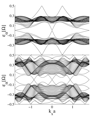
Figure 5: Quasi-energies in a cylindrical geometry highlighting edge states. The laser frequency is $\Omega=0.5t_{h}$, while the laser amplitude and Chern number are (upper panel) $A_{0}a=10,C=0$ and (lower panel) $A_{0}a=5,C=6.0$. It is the top phase ($C=0$) whose Hall response is discussed in detail in the text.

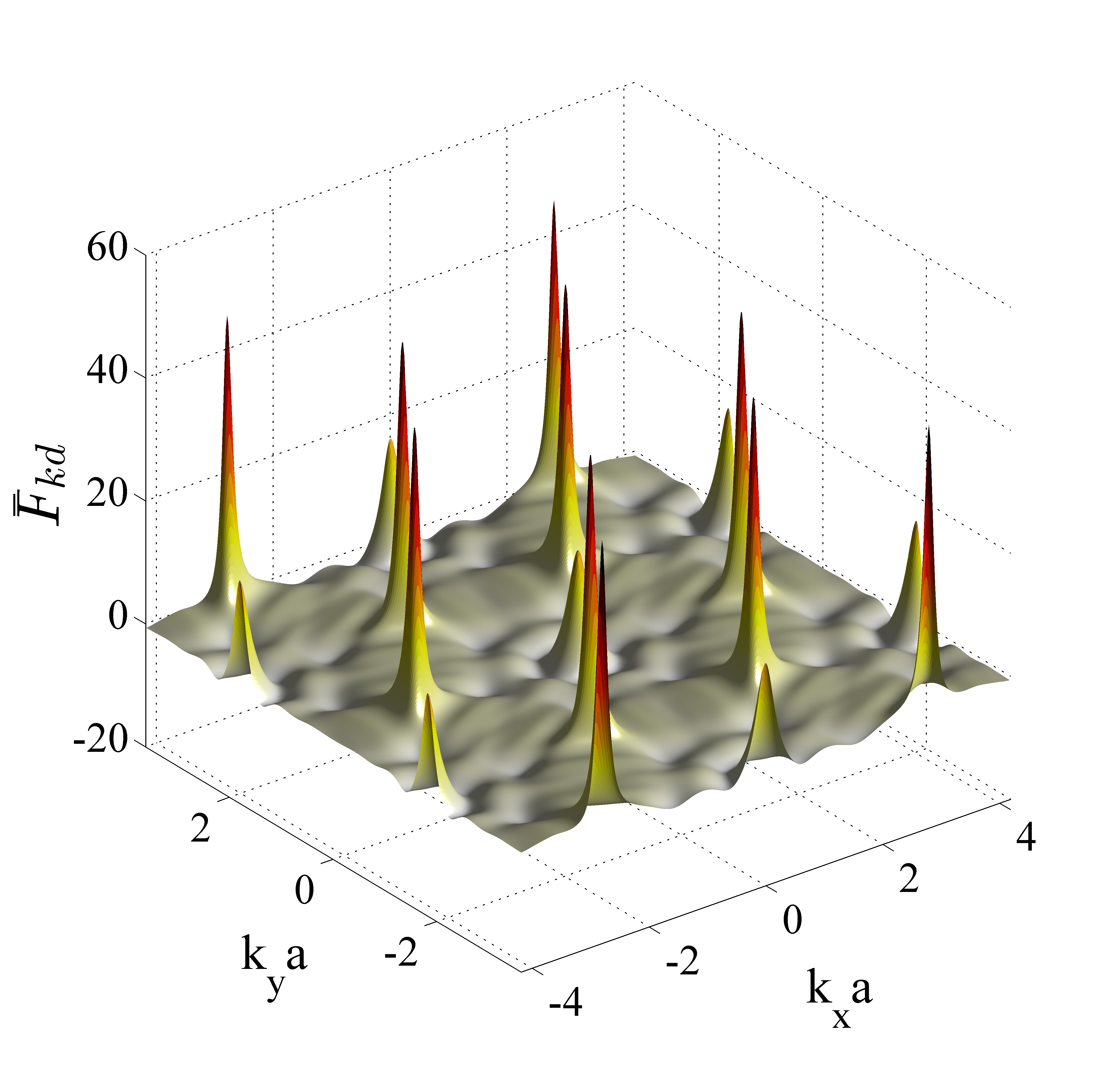
Figure 6: (color online) Time-averaged Berry curvature over 4 BZs for $\Omega=0.5t_{h},A_{0}a=10$ corresponding to a Chern number of $C=0$.

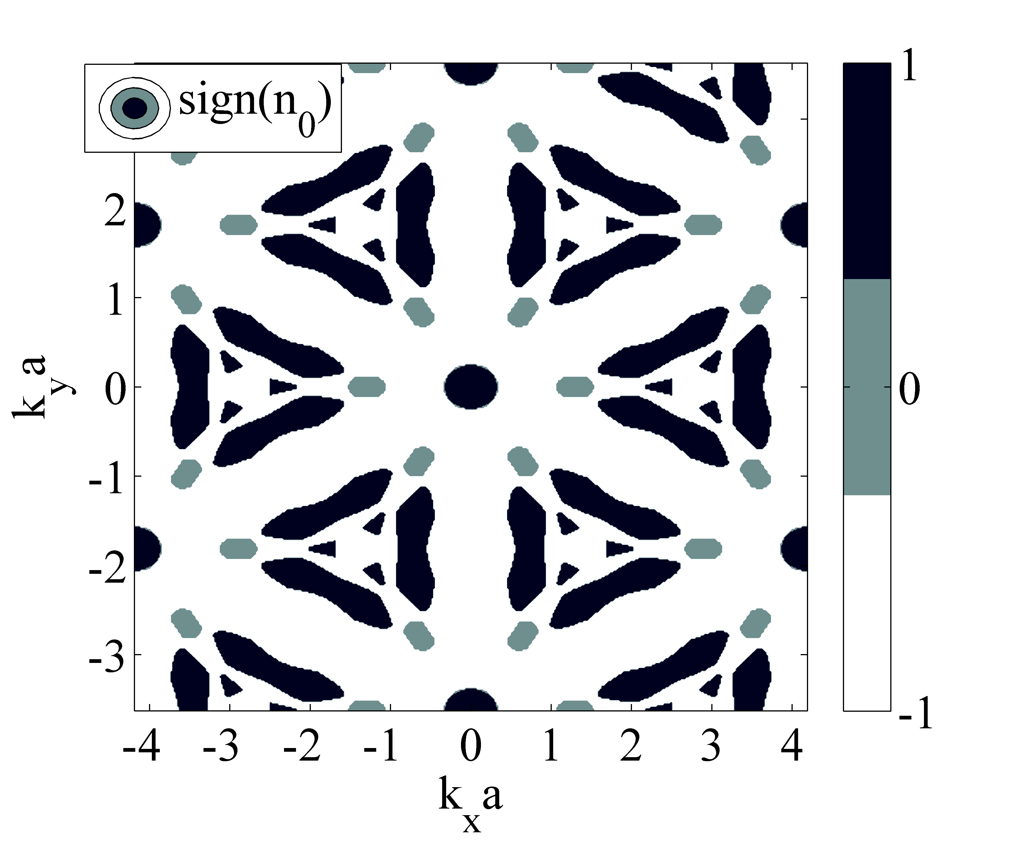
Figure 7: (color online) ${\rm Sign}(n_{0})$ in the dominant matrix element $M_{k}^{n_{0}}$ for $\Omega=0.5t_{h},A_{0}a=10,C=0$. The sign of the population imbalance ($\rho_{ku}-\rho_{kd}$) entering the Hall response follows this pattern.

One way to differentiate between this subtle matrix-element effect, and simply heating, where the latter will also give a low $\sigma_{xy}$, is by studying the temperature dependence. As the temperature is increased, one finds that the Hall conductivity actually increases (opposite to the heating case). This happens because the quasi-energy level separation near the Dirac points and around the circles is not the same, with the former being larger than the latter. Raising the temperature excites electrons to the ”down” level near the circles, while excitations to the ”up” level near the Dirac cones do not occur until higher temperatures. This results in a low temperature region where the Hall conductivity increases with temperature because in this regime as the temperature increases, the effective population imbalance between the two Floquet bands with opposite Berry curvature increases. This qualitative behavior is not special to these parameters, but holds for the entire topological phase where the only difference is the size of the circle in Fig. 4, and more generically is a signature of the fact that more than one scattering rate plays a dominant role in transport.

We now discuss this strong matrix element dependence in another phase of the FTI. We choose a much lower laser frequency, but larger laser amplitude ($\Omega=0.5t_{h},A_{0}a=10,C=0$) where one expects several band inversions as resonances involving $n=1\ldots 12$-photon processes are in principle allowed, although how visible these are, depends on the laser amplitude. The corresponding quasi-energy spectra and Berry-curvature are shown in Fig. 5 and 6 respectively.

For $A_{0}a=10$, $M_{k}^{n}$ has contributions from many $n$ where the dominant matrix element $M_{k}^{n_{0}}$ is such that $-4\lesssim n_{0}\lesssim 4$ in the BZ. Fig. 7 shows how the sign of $n_{0}$ varies through the BZ, where for $n_{0}=0$ or a positive integer, the population is primarily in the ”down” level at low temperatures, while $n_{0}$-negative gives a population primarily in the ”up” level. The sign of the population difference follows the pattern in Fig. 7, leading to a dc Hall conductivity that is not only small, but also has a non-monotonic temperature dependence. Changing the laser parameters in such a way as to stay within the same topological phase, simply changes the size of the pockets of ${\rm max}(n_{0})$ in the BZ, with no crossings or no new pockets appearing. Note that this particular phase is not a usual Chern insulator as $C=0$, yet the system does support edge states. Moreover, while we are studying the system in the bulk, and edges do not enter explicitly in our Kubo formula approach, yet we do pick up a non-zero Hall response coming from the non-zero Berry-curvature of the bulk bands.

While so far we have been mainly discussing the low frequency Hall response, we now make some general observations about the high frequency response. We find that for small amplitudes $A_{0}a\simeq{\cal O}(1)$, $\sigma_{xy}(\omega)$ is saturated by $\omega\sim\Omega$ (Fig. 1). On the other hand, for larger amplitudes, like the case just discussed ($A_{0}a\simeq{\cal O}(10)$), $\sigma_{xy}$ is non-zero over a larger range of frequencies (see Fig. 8), with the position and magnitude of the side-bands depending on the structure of $F_{k}^{m}$. This is highlighted in Fig. 9 where the structure in the total optical Hall conductivity plotted in Fig. 8 has been decomposed into those arising from separate Fourier components of $F_{k}$.

To understand the location of the peaks in $\omega$, it is convenient to look again at the low amplitude case ($\Omega=5.0t_{h},A_{0}a=1.5\&0.5$). Here only $F_{k}^{m=0,1}$ are dominant, but while for one ($A_{0}a=1.5$), $F_{k}^{m=1}$ is peaked at $\epsilon_{ku}-\epsilon_{kd}\ll\Omega$, for the other ($A_{0}a=0.5$), $F_{k}^{m=1}$ is peaked at $\epsilon_{ku}-\epsilon_{kd}\sim\Omega$. In fact $F_{k}^{m=0},F_{k}^{m=1}$ are respectively the Dirac cones and circles in Fig. 4. Thus a side-band appears at $\omega\sim|\epsilon_{ku}-\epsilon_{kd}-\Omega|\sim 0.75\Omega$ for the case of $A_{0}a=1.5,C=1$, while no such side-band is visible for $A_{0}a=0.5,C=3$. Similar arguments can be utilized to understand the peaks in the high frequency response for the large amplitude case shown in Figs. 8 and  9. Thus while the optical Hall conductivity at non-zero frequency $\sigma_{xy}(\omega\neq 0)$ is not a topological quantity, yet it is sensitive to the structure of the Berry curvature both in momentum and time.

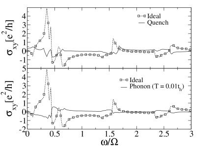
Figure 8: $\sigma_{xy}(\omega)$ for $\Omega=0.5t_{h},A_{0}a=10,C=0$. In comparison to the case of $\Omega=5.0t_{h},A_{0}a=1.5,0.5$, many side-bands are visible, and the response is sensitive to the distribution function over a larger frequency range $\omega$.

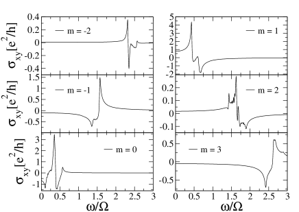
Figure 9: $\sigma_{xy}^{m}$ for $\Omega=0.5t_{h},A_{0}a=10,C=0$ and for an ideal distribution $\rho_{ku}-\rho_{kd}=1$. The peaks are at $\omega\sim|\epsilon_{ku}-\epsilon_{kd}-m\Omega|$ where the location of $k$ is determined by the peaks in $F_{k}^{m}$.

V Conclusions

In summary we have presented results for the optical Hall conductivity which can be measured in an all optical measurement such as Faraday rotation, as well as using leads. The low frequency Hall conductivity, even in steady-state with a reservoir, is remarkably sensitive to the topological phase, which is communicated through the structure of the system-reservoir matrix elements, resulting in steady-states with anomalous temperature dependence, and also opening up the possibility of manipulating the steady-state by suitable reservoir engineering Seetharam et al. (shed); Iadecola et al. (2015), for example by applying strain fields that modify the symmetries of the electron-phonon coupling. We also find that the high-frequency response acts as a spectroscopic tool for the Fourier components of the time-dependent Berry curvature.

We presented detailed results for the optical Hall response in three different phases of the FTI. One is where the Chern number coincided with the number of edge-states which were all in the center of the FBZ ($\Omega=5t_{h},A_{0}a=1.5,C=1$), the other where the Chern number does not equal the number of edge-states but rather equals the difference in the number of chiral edge-states above and below the Floquet band ($\Omega=5t_{h},A_{0}a=0.5,C=3$), while the third was one where $C=0$ ($\Omega=0.5t_{h},A_{0}a=10,C=0$), so that the band was not a conventional Chern insulator, yet the system supports edge states with the number of chiral edge modes above and below the band equal to each other (hence $C=0$). An interesting future direction of research is to compare the results presented here which were based on a bulk Kubo formula treatment, and which is sensitive to the bulk Berry-curvature, with a Landauer transport approach through a short sample where the leads determine the occupation of the Floquet states.

Acknowledgments: The authors thank Andrea Cavalleri and Takashi Oka for helpful discussions. This work was supported by the US Department of Energy, Office of Science, Basic Energy Sciences, under Award No. DE-SC0010821.

Appendix A Derivation of Floquet-Master equation

We assume that initially the system is in the ground state of graphene $|\Psi(t=0)\rangle=\prod_{k}|\psi_{\rm in,k}\rangle$, and we time-evolve the system according to $H$. For the closed system ($H_{c}=0$), this time-evolution can be studied exactly, while in the presence of phonons, we solve the problem by assuming a weak electron-phonon coupling, and a very fast bath so that a Floquet-Markov approximation can be made. This approach has been discussed in detail elsewhere Dehghani et al. (2014, 2015), however for completeness we briefly highlight the main steps. Let $W(t)$ be the full density matrix obeying $\frac{dW(t)}{dt}=-i\left[H,W(t)\right]$. In the interaction representation, $W_{I}(t)=e^{iH_{\rm ph}t}U^{\dagger}_{\rm el}(t,0)W(t)U_{\rm el}(t,0)e^{-iH_{\rm ph}t}$, where $U_{\rm el}(t,t^{\prime})=\prod_{k}U_{k}(t,t^{\prime})$ is the time-evolution operator for the electrons under a periodic drive where $U_{k}(t,t_{0})=\sum_{\alpha=u,d}e^{-i\epsilon_{k\alpha}(t-t_{0})}|\phi_{k\alpha}(t)\rangle\langle\phi_{k\alpha}(t_{0})|$ with $|\phi_{k\alpha}(t)\rangle,\epsilon_{k\alpha}$ being the quasi-modes and quasi-energies that obey $\biggl{[}H_{\rm el}-i\partial_{t}\biggr{]}|\phi_{k\alpha}\rangle=\epsilon_{k\alpha}|\phi_{k\alpha}\rangle$. We will follow the convention of restricting the quasi-energies to a Floquet Brillouin zone (FBZ), $-\Omega/2<\epsilon_{k\alpha}<\Omega/2$, and label the two quasi energy-levels such that $\epsilon_{ku}>\epsilon_{kd}$. Defining the electron reduced density matrix as the one obtained from tracing over the phonons, $W^{\rm el}={\rm Tr}_{\rm ph}W$, at ${\cal O}(H_{c}^{2})$ we need to solve,

$$\frac{dW^{\rm el}_{I}}{dt}=-{\rm Tr}_{\rm ph}\int_{t_{0}}^{t}dt^{\prime}\left[H_{c,I}(t),\left[H_{c,I}(t^{\prime}),W_{I}(t^{\prime})\right]\right]$$ (15)

We assume that at the initial time $t_{0}$, the electrons and phonons are uncoupled so that $W(t_{0})=W^{\rm el}_{0}(t_{0})\otimes W^{\rm ph}(t_{0})$, and that initially the electrons are in the post-quench state $|\Psi(t)\rangle=\prod_{k}U_{k}(t,0)|\psi_{\rm in,k}\rangle$. Thus, $W^{\rm el}_{0}(t)=|\Psi(t)\rangle\langle\Psi(t)|=\prod_{k}W^{\rm el}_{k,0}$ where

$$\!\!W^{\rm el}_{k,0}(t)=\!\!\!\sum_{\alpha,\beta=u,d}e^{-i(\epsilon_{k\alpha}-\epsilon_{k\beta})t}|\phi_{k\alpha}(t)\rangle\langle\phi_{k\beta}(t)|\rho_{k,\alpha\beta}^{\rm quench}$$ (16)

with $\rho_{k,\alpha\beta}^{\rm quench}=\langle\phi_{k\alpha}(0)|\psi_{{\rm in},k}\rangle\langle\psi_{{\rm in},k}|\phi_{k\beta}(0)\rangle$. Since the phonons are an ideal reservoir that stay in thermal equilibrium at temperature $T$ at all times, we write $W_{I}(t)=W^{\rm el}_{I}(t)\otimes e^{-H_{\rm ph}/T}/{\rm Tr}\left[e^{-H_{\rm ph}/T}\right]$ (we set $k_{B}=1$).

The most general form of the reduced density matrix for the electrons is $W^{\rm el}_{I}(t)=\prod_{k}\sum_{\alpha\beta}\rho_{k,\alpha\beta}(t)|\phi_{k\alpha}(t)\rangle\langle\phi_{k\beta}(t)|$ where in the absence of phonons, $\rho_{k,\alpha\beta}=\rho_{k,\alpha\beta}^{\rm quench}$ and are time-independent in the interaction representation. The last remaining step is to make the following three approximations Kohler et al. (2005); Kohn (2001); Hone et al. (2009): (a). $\rho_{k,\alpha\beta}$ are slowly varying as compared to the characteristic time scales of the reservoir (Markov approximation), (b) they are also slowly varying in comparison to the laser frequency so that the scattering rates can be averaged over one cycle of the laser (modified rotating wave approximation) and, (c) we are away from any topological transitions so that the spacing between quasi-energy levels is large as compared to the coupling to the bath ($|\epsilon_{ku}-\epsilon_{kd}-n\Omega|>D_{\rm ph}\lambda^{2},|n\Omega|>D_{\rm ph}\lambda^{2}$), under such conditions the off-diagonal matrix elements ($\rho_{kud}$) are small and can be dropped. These approximations lead to the rate equation, $\dot{\rho}_{k,\alpha\alpha}(t)=-\sum_{\beta=u,d}L^{k}_{\alpha\alpha;\beta\beta}\rho_{k,\beta\beta}(t)$ where $L^{k}_{\alpha\alpha,\beta\beta}$ are the scattering rates.

References

- Thouless et al. (1982) D. J. Thouless, M. Kohmoto, M. P. Nightingale, and M. den Nijs, Phys. Rev. Lett. 49, 405 (1982).
- Bellissard et al. (1994) J. Bellissard, A. van Elst, and H. Schulz‐ Baldes, Journal of Mathematical Physics 35 (1994).
- Avron et al. (1994) J. Avron, R. Seiler, and B. Simon, Communications in Mathematical Physics 159, 399 (1994).
- Klitzing et al. (1980) K. v. Klitzing, G. Dorda, and M. Pepper, Phys. Rev. Lett. 45, 494 (1980).
- Morimoto et al. (2009) T. Morimoto, Y. Hatsugai, and H. Aoki, Phys. Rev. Lett. 103, 116803 (2009).
- O’Connell and Wallace (1982) R. F. O’Connell and G. Wallace, Phys. Rev. B 26, 2231 (1982).
- Ikebe et al. (2010) Y. Ikebe, T. Morimoto, R. Masutomi, T. Okamoto, H. Aoki, and R. Shimano, Phys. Rev. Lett. 104, 256802 (2010).
- Crassee et al. (2011) I. Crassee, J. Levallois, A. L. Walter, M. Ostler, A. Bostwick, E. Rotenberg, T. Seyller, D. Van Der Marel, and A. B. Kuzmenko, Nature Physics 7, 48 (2011).
- Shimano et al. (2013) R. Shimano, G. Yumoto, J. Y. Yoo, R. Matsunaga, S. Tanabe, H. Hibino, H. Morimoto, and H. Aoki, Nature Comm. 4, 1841 (2013).
- Haldane (1988) F. D. M. Haldane, Phys. Rev. Lett. 61, 2015 (1988).
- Oka and Aoki (2009) T. Oka and H. Aoki, Phys. Rev. B 79, 081406 (2009).
- Inoue and Tanaka (2010) J. Inoue and A. Tanaka, Phys. Rev. Lett. 105, 017401 (2010).
- Kitagawa et al. (2010) T. Kitagawa, E. Berg, M. Rudner, and E. Demler, Phys. Rev. B 82, 235114 (2010).
- Lindner et al. (2011) N. H. Lindner, G. Refael, and V. Galitski, Nature Physics 7, 490 (2011).
- Gu et al. (2011) Z. Gu, H. A. Fertig, D. P. Arovas, and A. Auerbach, Phys. Rev. Lett. 107, 216601 (2011).
- Katan and Podolsky (2013) Y. T. Katan and D. Podolsky, Phys. Rev. Lett. 110, 016802 (2013).
- Jotzu et al. (shed) G. Jotzu, M. Messer, R. Desbuquois, M. Lebrat, T. Uehlinger, D. Greif, and T. Esslinger, arXiv:1406.7874 (unpublished).
- Karch et al. (2010) J. Karch, P. Olbrich, M. Schmalzbauer, C. Zoth, C. Brinsteiner, M. Fehrenbacher, U. Wurstbauer, M. M. Glazov, S. A. Tarasenko, E. L. Ivchenko, D. Weiss, J. Eroms, R. Yakimova, S. Lara-Avila, S. Kubatkin, and S. D. Ganichev, Phys. Rev. Lett. 105, 227402 (2010).
- Karch et al. (2011) J. Karch, C. Drexler, P. Olbrich, M. Fehrenbacher, M. Hirmer, M. M. Glazov, S. A. Tarasenko, E. L. Ivchenko, B. Birkner, J. Eroms, D. Weiss, R. Yakimova, S. Lara-Avila, S. Kubatkin, M. Ostler, T. Seyller, and S. D. Ganichev, Phys. Rev. Lett. 107, 276601 (2011).
- Wang et al. (2013) Y. H. Wang, H. Steinberg, P. Jarillo-Herrero, and N. Gedik, Science 342, 453 (2013).
- Rechstman et al. (2013) M. Rechstman, J. Zeuner, Y. Plotnik, Y. Lumer, D. Podolsky, F. Dreisow, S. Nolte, M. Segev, and A. Szameit, Nature (London) 496, 196 (2013).
- Rudner et al. (2013) M. S. Rudner, N. H. Lindner, E. Berg, and M. Levin, Phys. Rev. X 3, 031005 (2013).
- Kundu et al. (2014) A. Kundu, H. A. Fertig, and B. Seradjeh, Phys. Rev. Lett. 113, 236803 (2014).
- Carpentier et al. (2015) D. Carpentier, P. Delplace, M. Fruchart, and K. Gawedzki, Phys. Rev. Lett. 114, 106806 (2015).
- Dehghani et al. (2015) H. Dehghani, T. Oka, and A. Mitra, Phys. Rev. B 91, 155422 (2015).
- Datta (1997) S. Datta, Electronic Transport in Mesoscopic Systems, Cambridge University Press (1997).
- Torres et al. (2014) L. E. F. F. Torres, P. M. Perez-Piskunow, C. A. Balseiro, and G. Usaj, Phys. Rev. Lett. 113, 266801 (2014).
- Farrell and Pereg-Barnea (shed) A. Farrell and T. Pereg-Barnea, arXiv:1505.05584 (unpublished).
- Oka and Aoki (2011) T. Oka and H. Aoki, J. Phys.:Conf. Ser. 334, 012060 (2011).
- Suzuura and Ando (2002) H. Suzuura and T. Ando, Phys. Rev. B 65, 235412 (2002).
- Ando (2006) T. Ando, Journal of the Physical Society of Japan 75, 124701 (2006).
- Kohler et al. (2005) S. Kohler, J. Lehmann, and P. Hänggi, Phys. Rep. 406, 379 (2005).
- Kohn (2001) W. Kohn, J. Stat. Phys. 103, 417 (2001).
- Hone et al. (2009) D. W. Hone, R. Ketzmerick, and W. Kohn, Phys. Rev. E 79, 051129 (2009).
- Dehghani et al. (2014) H. Dehghani, T. Oka, and A. Mitra, Phys. Rev. B 90, 195429 (2014).
- Seetharam et al. (shed) K. I. Seetharam, C.-E. Bardyn, N. H. Lindner, M. S. Rudner, and G. Refael, arXiv:1502.02664 (unpublished).
- Iadecola et al. (2015) T. Iadecola, T. Neupert, and C. Chamon, Phys. Rev. B 91, 235133 (2015).