Collective Fluctuations in models of adaptation

Abstract

The dynamics of adaptation is difficult to predict because it is highly stochastic even in large populations. The uncertainty emerges from number fluctuations, called genetic drift, arising in the small number of particularly fit individuals of the population. Random genetic drift in this evolutionary vanguard also limits the speed of adaptation, which diverges in deterministic models that ignore these chance effects. Several approaches have been developed to analyze the crucial role of noise on the expected dynamics of adaptation, including the mean fitness of the entire population, or the fate of newly arising beneficial deleterious mutations. However, very little is known about how genetic drift causes fluctuations to emerge on the population level, including fitness distribution variations and speed variations. Yet, these phenomena control the replicability of experimental evolution experiments and are key to a truly predictive understanding of evolutionary processes. Here, we develop an exact approach to these emergent fluctuations by a combination of computational and analytical methods. We show, analytically, that the infinite hierarchy of moment equations can be closed at any arbitrary order by a suitable choice of a dynamical constraint. This constraint regulates (rather than fixes) the population size, accounting for resource limitations. The resulting linear equations, which can be accurately solved numerically, exhibit fluctuation-induced terms that amplify short-distance correlations and suppress long-distance ones. Importantly, by accounting for the dynamics of sub-populations, we provide a systematic route to key population genetic quantities, such as fixation probabilities and decay rates of the genetic diversity. We demonstrate that, for some key quantities, asymptotic formulae can be derived. While it is natural to consider the process of adaptation as a branching random walk (in fitness space) subject to a constraint (due to finite resources), we show that other noisy traveling waves likewise fall into this class of constrained branching random walks. Our methods, therefore, provide a systematic approach towards analyzing fluctuations in a wide range of population biological processes, such as adaptation, genetic meltdown, species invasions or epidemics.

Many important evolutionary and ecological processes rely on the behavior of a small number of individuals that have a large dynamical influence on the population as a whole. This is, perhaps, most obvious in the case of biological adaptation: Future generations descend from a small number of currently well-adapted individuals. The genetic footprint of the large majority of the population is wiped out over time by the fixation of more fit genotypes. These dynamics can be visualized as a traveling wave in fitness space, see Fig. 1A. At any time, the currently most fit “pioneer” individuals reside in the small tip of the wave. As time elapses, the wave moves towards higher fitness and the formerly rare most fit individuals dominate the population. By that time, however, a new wave tip of even more fit mutants has formed and the cycle of transient dominance continues.

The principle of “a few guiding the way for many” also characterizes the motion of flocks of birds, which can be controlled by just a few leaders, or the expansion of an invasive species, which depends on pioneers most advanced into the virgin territory. The overall dynamics of these processes can become highly erratic even in large populations because the behavior of the entire population is influenced by strong number fluctuations, called genetic drift, occurring in the small subset of “pioneer” individuals.

Such propagation processes with an extreme sensitivity of noise have also been called “pulled” waves, because they are pulled along by the action of the most advanced individuals . If one ignores the fluctuations at the population level and is interested only in the expected dynamics of the population, one might be tempted to simply ignore genetic drift in models of pulled waves. However, it turns out that mean-field models ignoring genetic drift drastically overestimate the speed of traveling waves, to the point that they predict an ever accelerating rather than a finite speed of adaptation. It took 70 years since the first formulation of traveling wave models by Fisher and Kolomogorov, to realize that genetic drift influences both the expectation and the variation in singular ways tsimring1996rna ; brunet1997shift .

The expected behavior of pulled waves has since been analyzed at great length. Many results were first obtained for waves of invasion, noisy versions of the classical “FKPP” model by Fisher, Kolmogorov, Petrovskii, Piskunov van2003front . In recent years, however, there has been a particularly strong research focus on models of adaptation. These models aroused widespread interest because they can be applied to several types of data, including genomic data derived from experimental evolution experiments and from natural populations that undergo rampant adaptation, such as bacteria and viruses neher2013genetic . We now have analytical predictions for a number of valuable analytical or semi-analytical results for observables such as the mean speed, probability of fixation, distribution of fixed mutations in the asymptotic regime of large populations neher2013genetic . The great value of these results is that they show and rationalize which parameter combination chiefly influence the dynamics, and through which functional form. Importantly, it has been generally found that the overall dynamics depends logarithmically on population size and mutation rate. The weak functional dependence is in fact at the root of universality observed in many such wave models: These predictions are independent of the precise details of the models, including the form of the non-linear population size regulation.

The basic challenge in analyzing noisy traveling arise from an essential non-linearity that is required to control population growth. Ignoring such a dynamical control of the population size leads to long-term exponential growth or population extinction. Progress in describing the mean behavior of front-sensitive models has been achieved by at least three different approaches: One can either heuristically improve the mean-field dynamics by setting the net growth rate equal to zero in regions where the population densities are too small tsimring1996rna . Such an ad-hoc approach, based on a growth rate cut-off, correctly reproduces the wave speed to the leading order but does not reveal other universal next-to-leading order corrections or the wave diffusion constant. One can also invoke a branching-process approximation for the tip of the wave, thereby neglecting effects of the non-linear population size control, and then match this linearized description with a deterministic description of the bulk of the population rouzine2003solitary ; desai2007beneficial ; rouzine2008traveling ; schiffels2011emergent ; good2012distribution . Finally, there is also the possibility to invoke a particular dynamical constraint with the property that the dynamics exhibits a closed linear equation for the first moment. Importantly, this method, which has been called “model tuning” hallatschek2011noisy ; good2012distribution ; geyrhofer2013stochastic , reproduces the universal features of noisy traveling waves, which are independent of the chosen population control, ultimately because of the weakness of the population size dependence.

While understanding the mean behavior of noisy traveling waves has been an important achievement, the actual stochastic dynamics is characterized by pronounced fluctuations at the population level. No two realizations of an evolution experiment, for instance, will exhibit the same time-dependent fitness distribution because of the chance effects involved in reproduction and mutations. Measuring the mean behavior requires many replicates in which the entire environment is accurately reproduced. Even if one has access to many replicates, as is possible in highly parallelized well-mixed evolution experiments, one can potentially learn a lot from the variability between replicates. Thus, a predictive understanding of the variability in evolutionary trajectories would greatly improve our quantitative understanding of how evolution works.

Some exact results on fluctuations at the population level are available for a special model of FKPP waves brunet2006phenomenological . Still, we currently lack a systematic approach that can be applied to a wide range of models. Here, we fill this gap by extending the method of “model tuning” hallatschek2011noisy to the analysis of higher correlation functions: We show that it is possible to choose a constraint in such a way that the hierarchy of moments is closed at any desired level. The resulting linear equations can be solved numerically and are amenable to asymptotic analytical techniques. As an important application of this approach, we show how the coalescence time can be computed within traveling wave models.

Although our main results are applicable to a wide range of models, we focus our attention on simple models of adaptation. Beyond simply grounding our discussion, there are two reasons to focus on these models. On the one hand, models of adaptation are simply important and have become an indispensable tool as a null model for evolutionary dynamics in microbial population. On the other hand, models of adaptation manifestly exhibit a particular mathematical structure, which we call constrained branching random walks. As we will argue below, this mathematical structure, to which all our formal results apply, can be identified as the essence of a wide range of models arising in physics, ecology and evolution.

I Models of adaptation as Constrained Branching Random Walks

Darwinian adaptation spontaneously emerges from the processes of mutation, reproduction and competition, and these features need to be mirrored in any model of adaptation. In models, spontaneous mutations can be represented by a stochastic jump process in a “fitness space”. Reproduction is naturally described by a branching process by which individuals give birth at certain fitness-dependent rates allen2003introduction ; haccou2005branching . In combination, reproduction and mutations thus generate a branching random walk allen2003introduction ; haccou2005branching , which by itself would lead to diverging population sizes. To avoid this unrealistic outcome, models of adaptation also encode a constraint on population sizes to account for the competition for finite resources. The resulting process is a branching random walk subject to a global constraint, which we now frame mathematically.

The state of the population at time $t$ is described by a function $c_{t}(x)$ representing the number density of individuals with fitness $x$. In this context, fitness refers to an individual’s net-growth rate in the absence of competition for resources. The population is assumed to evolve in discrete timesteps of size $\epsilon$, which is eventually sent to zero in order to obtain a continuous-time Markov process. Each timestep consists of two sub-steps. The first substep realizes reproduction and mutations and the second substep implements competition.

I.1 First substep: Reproduction and mutations

The combined effect of reproductions and mutations can be described by the stochastic equation

$$\tilde{c}_{t+\epsilon}-c_{t}=\epsilon\mathcal{L}_{t}c_{t}+\sqrt{\epsilon bc_{t}}\,\eta_{t}\;,$$ (1)

which takes the number density $c_{t}$ to an intermediate value $\tilde{c}_{t+\epsilon}$. The term $\epsilon\mathcal{L}c_{t}$ represents the expected change in density due to reproduction and mutations. This term is linear in the number density because the number of offspring and mutants per timestep is proportional to the current population density. The term $\sqrt{\epsilon bc_{t}}\,\eta_{t}$ represents all sources of noise arising in this setup. We will now discuss separately the precise meaning of both terms, and give natural alternatives for their form.

The Liouville operator $\mathcal{L}_{t}$ depends on how the mutational process is modeled, and various examples are discussed in the following. A particularly simple example is provided by $\mathcal{L}_{t}=D\partial_{x}^{2}+x-x_{0}(t)$, which has been used to model asexual evolution on a continuous fitness landscape tsimring1996rna ; hallatschek2011noisy . Here, the diffusion constant $D$ quantifies the fitness variance per generation, generated by an influx of novel mutations. To account for the notorious observation that most mutations are deleterious, a drift term $-v_{d}\partial_{x}$ is often included. The linear “reaction” term $x-x_{0}$ in $\mathcal{L}_{t}$ simply accounts for the fact that individuals with higher growth rate $x$ grow faster. The term $x_{0}(t)$ refers to the mean fitness of the population, which separates the population with a positive net growth rate $x>x_{0}$ from the less fit part of the population with $x<x_{0}$.

One cannot generally assume that (biased) diffusion is a good model for discrete mutational events because of the presence of the reaction term favoring highly fit individuals. The diffusion approximation requires that mutation rates are higher than the typical fitness effects of novel mutations. This may apply to rapidly mutating organisms, such as viruses, or close to a dynamic mutation-selection balance goyal2012dynamic ; neher2013coalescence . It may also effectively apply in island models with low migration rates, where the fitness effect of a mutation is reduced by potentially low migration rates. But, in well-mixed populations, the diffusion approach breaks down when beneficial mutation rates are much smaller than their typical effect, which has been confirmed for a number of microbial species when they adapt to new environments perfeito2007adaptive ; gordo2011fitness ; levy2015quantitative . More generally, asexual adaptation may, therefore, be cast into the form

$$\mathcal{L}_{t}=\mathcal{M}_{t}+x-x_{0}(t)\;,$$ (2)

where the mutational process is described by the operator $\mathcal{M}_{t}$, which conserves particle numbers, i.e., describes a pure jump process. For instance, one may have one of the time-independent kernels

$$\{\mathcal{M}_{t}c_{t}\}(x)\sim\left\{\begin{matrix}D\partial_{x}^{2}c_{t}(x)\;,&\text{Diffusion Kernel}\\ \mu\left[c_{t}(x-s)-c_{t}(x)\right]\;,&\text{Staircase Kernel}\\ \int\mu(y)\left[c_{t}(x-y)-c_{t}(y)\right]dy\;,&\text{General Mutational Kernel}\end{matrix}\;\right.$$ (3)

Here $\mu$ is a mutation rate and $s$ is a characteristic scale for the mutational effect. The diffusion kernel is the simplest of these kernels because it is characterized by only one compound parameter, the diffusion constant $D=\mu s^{2}$, rather than two in the Staircase Kernel or an entire function $\mu(y)$ in the general case.

The stochastic term $\sqrt{b\epsilon c_{t}}\eta_{t}$ in equation (1) accounts for all random factors that influence the reproduction process. The function $\eta_{t}(x)$ represents standard white noise, i.e. a set of delta correlated random numbers,

$$\overline{\eta_{t}(x)\eta_{t^{\prime}}(y)}=\delta(x-y)\delta_{tt^{\prime}}\;,$$ (4)

where $\overline{f}$ denotes the ensemble average of a random variable $f$, and $\delta(x)$ and $\delta_{ij}$ are the Dirac delta function and the Kronecker delta, respectively. The amplitude $\propto\sqrt{\epsilon bc_{t}}$ of the noise term in Eq.  (1) is typical for number fluctuations: Due to the law of large number, the expected variance in population numbers from one timestep to the next is proportional to the number $\epsilon c_{t}$ of expected births or deaths during one timestep. The numerical coefficient $b$ is the variance in offspring number per individual. For instance, when we assume that offspring have nearly matching division and death rates one finds $b=2$. The variance in offspring number is typically assumed to be of order one, but could become much larger if offspring distributions are highly-skewed, as it is the case when few individuals produce most of the offspring hedgecock2011sweepstakes .

I.2 Second substep: Population size constraint

Because the reproduction step generally changes population numbers, another sub-step, following the branching process, is required to enforce a constant population size ,

$$1=\int_{x}\frac{1}{N}c_{t}(x)\;.$$ (5)

In most models and experiments gerrish1998fate ; desai2007speed , this step is realized by a random culling of the population: individuals are eliminated at random from the population until the population size constraint is restored. Mathematically, the population control step can be cast into the form

$$c_{t+\epsilon}=\tilde{c}_{t+\epsilon}(1-\lambda)\;,$$ (6)

where $\lambda$ represents the fraction of the population that has to be removed to comply with the population size constraint. The second sub-step completes the computational timestep, and takes the concentration field from the intermediate state $\tilde{c}_{t+\epsilon}$ to the properly constrained state $c_{t+\epsilon}$.

The above standard model of adaptation with fixed population size represents a branching random walk subject to the constraint that the total population size is fixed. Enforcing this constraint leads to the non-linearity that makes the associated model difficult to solve.

Note that, in the above formulation, it is assumed that all noise comes from birth-death processes. We have ignored, for simplicity, additional sources of noise due to, e.g. the mutational jump processes, which are sub-dominant in large populations.

I.3 Generalization to arbitrary linear constraints

While it is necessary to constrain the population dynamics to avoid an exponential run-away, there is no particular biological reason to strictly fix the population size - in fact, most population sizes fluctuate over time frankham1995effective . As we will see, there are, however, mathematical reasons to consider constraints of particular form, which greatly simplify the analysis.

As a key step towards these tuned models, we note the fixed population size constraint Eq. (5) can be viewed as one member of a whole class of linear constraints,

$$1=\int_{x}u_{t}(x)c_{t}(x)\equiv\langle u_{t}\mid c_{t}\rangle\;.$$ (7)

that one could formulate with the help of a suitable weighting function $u_{t}(x)$. Any such constraint will be able to limit the population size, and thus defines, together with the Liouvillean $\mathcal{L}$, a particular model of adaptation. Our main result will be the observation that there are an entire set of weighting functions for which the dynamics of the model becomes simple (cf. Sec. III).

Note that one recovers the fixed population size constraint of one chooses the weighting function $u_{t}(x)$ to be a constant, $u=N^{-1}$. For any other choice, the population size will not be fixed. At best, one obtains a steady state with a population size fluctuating around its mean value, $\overline{N}_{t}$, which may change depending on the time-dependence imposed on the weighting function $u_{t}$. Note that culling is does not discriminate among individuals of different fitness. It is only the amount of culling that depends on the distribution and type of individuals if $u_{t}(x)$ is $x$–dependent.

II Invasion waves as constrained branching random walks

One advantage of using the general form Eq. (7) for a global constraint is that many types of traveling waves arising in ecology and evolution can be cast in the same mathematical form, if an appropriate Liouville operator and weighting function are used.

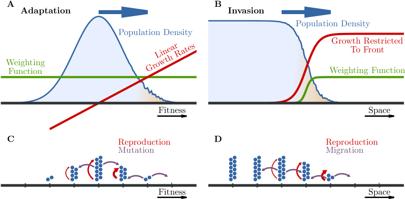
Figure 1: Models of adaptation and invasion. Illustration of the essential features of two types of noisy traveling waves: A Well-mixed models of asexual adaptation generate waves that travel across fitness landscapes towards higher fitness. B Models of species invasions, range expansions or epidemics generate waves that propagate in real space. Both types of waves can be viewed as emerging from constrained branching random walks. The state of the traveling wave is described by a (fluctuating) population density shown in blue. A branching process is generated by linear net-growth rates and a jump process. In the case of adaptive waves, individuals reproduce according to their current fitness and jump due to spontaneous mutations (C). By contrast, the jump process in invasion waves is generated by random movements according to some dispersal kernel, and density-dependent growth rates lead to an effective location dependence of the growth rates (D). A global constraint ensures a finite population size and depends on a weighting function $u_{t}(x)$ indicated in green. Note that for conventional models of adaptation with fixed population size, the growth rates are increasing with fitness and the weighting function is a constant. By contrast, for models of species invasion or range expansion without Allee effect hallatschek2008gene , the growth rates and weighting function have a sigmoidal shape, saturating in the tip of the wave. This ensures that individuals in the tip of the wave have the highest growth rates (because of least competition) and that their total number stays finite.

We would like to give an example of this assertion. Fig. 1b illustrates the expansion of a population in a real landscape, which may describe an advantageous gene spreading through a population distributed in space, or the invasion of virgin territory by an introduced species. Models of such real-space waves require the following features: i) populations reproduce and die “freely” in the tip of the wave, where population densities are small, ii) individuals move in real-space according to some jump process and iii) the net-growth vanishes in the bulk of the wave, where resources are sparse.

Features i) and ii) again generate a branching-random walk in the tip of the wave, however, according to different position-dependent growth and jump rates than in the case of evolution. Feature iii) requires a finite population size in the tip of the wave. This non-linearity keeps the branching-random walk away from proliferating to infinite densities, where mean-field models apply.

To generate an adequate branching-random walk, one has to use an appropriate Liouville operator. In one dimensions, one can choose, for instance,

$$\mathcal{L}_{t}=\mathcal{M}_{t}+s\,\Theta(x-x_{0}(t))\;.$$ (8)

Now, $x$ refers to the location in one-dimensional real space. $x_{0}$ refers to the position of the cross-over to the bulk of the wave. The operator $\mathcal{M}_{t}$ generates a jump process. In the simplest case, again, the jump process may be approximated by a diffusive process, $\mathcal{M}_{t}c=D\partial_{x}^{2}c$. The growth term does not need to be modeled by a strict step-function, any sigmoidal function works in the limit of large population sizes brunet1997shift . Importantly, the net reproduction rates monotonously increase in $x$ and saturates at some finite value $s$ at $x=O(1)$. Finally, to limit the population size in the front of the wave, we need to use a non-constant weighting function $u(x,t)$ in the global constraint, for instance, $u_{t}(x)=\frac{1}{N}\theta(x-x_{0})$, which ensures that the growth region contains precisely $N$ individuals.

The qualitative difference between the traveling waves in real and fitness space turns out to rely on the growth rates in the nose of the wave: While growth rates are saturating in the case of real-space waves, it is increasing without bound in the case of waves of adaptation. This makes models of adaptation even more sensitive to the effects of noise to the extent that a mean-field limit (neglecting noise) does not even yield finite velocity waves. Noise serves a crucial function in these models as it is required to regularize the wave dynamics. These waves have therefore been called “front-regularized waves” cohen2005fluctuation .

III Summary of Main Formal Results

In the same way as exemplified above for models of adaptation and invasion, one can frame many other eco-evolutionary scenarios, in their essence, as constrained branching random walks. These models are, ultimately, defined by an operator $\mathcal{L}_{t}$ generating the branching-random walk and a weighting function $u_{t}$ defining the global constraint. In this paper, we show that, in fact, for any given $\mathcal{L}_{t}$ there are natural ways of choosing the weighting function. The associated models, which we call tuned models, have desirable properties, including closed and linear moment equations, greatly facilitating their analysis.

We first state our main results on how to construct tuned models at any desired level of moments. We will then provide an interpretation of these tuned models and provide simulation results, which we compare to fixed population size models. Detailed analytical derivations are given in later sections.

To characterize fluctuations in the makeup of the population it is convenient to consider the so-called $n$-point correlation function $\overline{C}^{(n)}$, which is the noise-average of the product

$$C^{(n)}(x_{1},\dots,x_{n};t) \equiv \prod_{j=1}^{n}c(x_{j};t)\;,$$ (9)

of $n$ number density fields, $c(x_{j};t)$, evaluated at the same time $t$ at various locations ${x_{j}}$. Note that, here and henceforth, we use the notations $f_{t}(x)$ and $f(x;t)$ for a space and time-dependent function interchangeably.

From many studies over the last 15 years, we know a lot about the first moment, $\overline{C}^{(1)}(x;t)$, of several models of noisy traveling waves. This provides access to the expected shape and velocity of the traveling wave, as well as the expected fate of individual mutations, or sub-populations. However, wave shape and velocity fluctuations, as well, as the decay of genetic diversity requires access to higher moments, $n>1$, for which there is no systematic approach so far.

Our main result is that the dynamics of the $n^{\text{\tiny th}}$ moment (and of all lower moments) becomes analytically accessible if one chooses in the global constraint Eq. (7) the weighting function $u_{t}$ to have the form

$$u^{(n)}(x;t)=\frac{2w(x;t)}{b(n+1)}$$ (10)

for any positive integer $n$, where $w(x;t)$ satisfies

$$-\partial_{t}w=\left[\mathcal{L}^{\dagger}+\mathcal{\gamma}(t)-w\right]w$$ (11)

with the adjoint operator $\mathcal{L}^{\dagger}$ of $\mathcal{L}$. The arbitrary function $\gamma(t)$ controls the mean total population size as a function of time.

For the special weighting function Eq. (10), the equation of motion for the $n^{\text{\tiny th}}$ moment becomes closed and linear,

$$\partial_{t}\overline{C}^{(n)}=\sum^{n}_{j=1}\left.\left(\mathcal{L}+\gamma(t)-\frac{2n}{n+1}w\right)\right|_{x_{j}}\overline{C}^{(n)}+\frac{2}{n+1}\sum_{j=1}^{n}\sum_{k=j+1}^{n}\delta(x_{j}-x_{k})\langle w\mid\overline{C}^{(n)}\rangle_{k}\;.$$ (12)

The resulting models may be called tuned, because for all other choices of the weighting function, the equation of motion for $\overline{C}^{(n)}$ involves $\overline{C}^{(n+1)}$ resulting in an infinite hierarchy of moments. The moment closure of the tuned models is exact and not due to a truncation or approximation of higher moments. The two terms $\propto w$ are fluctuation-induced terms. The last, positive term generates correlations at equal space arguments, which are then dissipated by the first, strictly negative, term over longer time scales. The positive term exists only for $n>1$ and indicates that the effect of genetic drift on higher moments is more complicated than a cut-off in the growth term.

Moreover, examining the behavior of differently labeled, but otherwise identical, subpopulations shows that tuned models can be interpreted naturally in the framework of population genetics. First, the weighting function of all tuned models is a fixation probability function: The probability that descendants of individuals at location $x$ and time $t$ will take over the population on long times is given precisely by $u^{(n)}(x;t)=2w(x;t)/b(n+1)$ in the model tuned for the $n^{\text{\tiny th}}$ moment. It is remarkable, in this context, that equation Eq. (11) for $w(x;t)$ is precisely the equation governing the survival probability of an unconstrained branching random walk fisher2013asexual , with $b=2$.

Secondly, the higher moments provide access to the statistics of the genetic makeup of the population. According to the principle tenet of population genetics that, without mutations, the genetic diversity of a population decreases with time: fixation and extinction of subtypes needs to be maintained by an appropriate influx of mutations. The decay of genetic diversity fundamentally depends on higher moments – the first moment captures fixation probabilities but not the time to fixation.

The decay of genetic diversity in the absence of mutations can be quantified by the cross-correlation function

$$\overline{C}^{(n)}_{i_{1},\dots,i_{n}}(x_{1},\dots,x_{n};t) \equiv \overline{\prod_{j=1}^{n}c_{i_{j}}(x_{j};t)}\;,$$ (13)

between subtypes $i_{1},\dots,i_{n}$. Here, the number densities $c_{i}(x;t)$ is the number density field of type $i$. The sum of all sub-types makes up the total population, $c(x;t)=\sum_{i}c_{i}(x;t)$.

If all $i_{j}$ are different and $n>1$, it is clear that $\overline{C}^{(n)}_{i_{1},\dots,i_{n}}$ must continuously decay in the absence of mutations because one of the subtypes will take over in the presence of random genetic drift. The case $n=2$ is the most prominent one: $\overline{C}^{(2)}_{1,2}(x,x;t)$ is proportional to the so-called heterozygosity at location $x$ and $t$, which is the probability that two individuals sampled with replacement are of different type wakeley2009coalescent .

Now it turns out that, in the $n^{\text{\tiny th}}$ -tuned model, the cross-correlation function can be expressed in the simple form

$$\overline{C}^{(n)}_{i_{1},\cdots,i_{n}}=\prod_{k=1}^{n}f_{i_{k}}(x_{i_{k}};t)$$ (14)

with $f_{i_{k}}(x_{i_{k}};t)$ satisfying a one-dimensional linear equation

$$\partial_{t}f_{i_{k}}(x;t)=\left(\mathcal{L}+\gamma(t)-\frac{2n}{n+1}w\right)f_{i_{k}}(x;t)$$ (15)

subject to the initial conditions $f_{i_{k}}(x;0)=c_{i_{k}}(x;0)$.

Notice that the decay of genetic diversity in the $n^{\text{\tiny th}}$ -tuned model is described by the spectrum of the operator appearing on the right-hand side of Eq. (15), which also occurs in Eq. (12) describing the fluctuations of the total population. Consistent with our population genetic interpretation, one can show quite generally that this operator only has decaying relaxation modes (see Fig. 8).

We consider Eqs. (14) and (15) to be our results with the most immediate applicability because they provide a feasible approach to resolving a key question in population genetics (maintenance and decay of genetic diversity) that relies on having access to higher moments.

III.1 Remarks

The above formalism includes the case $n=1$ (closed first moment) presented in Ref. hallatschek2011noisy (in which the tuned weighting function $u^{(1)}$ was denoted by $u_{*}$).

In constrained random walk models, one can generally retrieve lower moments from higher moments by contraction with the weighting function $u$,

$$\langle u\mid C^{(n)}\rangle_{x_{k}} = c(x_{1};t)\dots\left(\int_{x_{k}}u(x_{k};t)c_{t}(x_{k};t)\right)\dots c(x_{n};t)$$ (16)

$$= c(x_{1};t)\dots c(x_{k-1};t)\,1\,c(x_{k+1};t)\dots c(x_{n-1};t)$$

$$\equiv C^{(n-1)}(\backslash x_{k};t)\;,$$

where we invoked the global constraint Eq. (7) in going from the second to the third line. To simplify the notation, we have here introduced the short hand $C^{(n-1)}(\backslash x_{m};t)$ to denote $C^{(n-1)}(x_{1},\dots,x_{m-1},x_{m+1},\dots,x_{n};t)$, i.e., that the $m$th space variable should be omitted in the arguments.

The contraction rule Eq. (16) also shows that contraction in the last term in the dynamical equation for $C^{(n)}$ simply generates the next lower moment $C^{(n-1)}$. Moreover, if one obtains the $n^{\text{\tiny th}}$ moment by solving Eq. (12), one generally has access to all lower-rank moments as well (but not to the larger moments). Thus, the model tuned to be linear at the $n^{\text{\tiny th}}$ moment gives access to all moments up to and including the $n^{\text{\tiny th}}$ .

It is remarkable that the governing equations for $w$ and $\overline{C}^{(n)}$ are independent of the offspring number variation $b$. The only effect of $b$ is to reduce the fixation probability $u^{(n)}\propto b^{-1}$ and scale up the population sizes $\overline{C}^{(n)}\propto b^{n}$. This means in particular that noise-induced terms $\propto w$ in the moment equation are not scaled by $b$, and thus do not become small in the small noise limit. The lack of a potentially small parameter has important consequences for the use of perturbation theory in this context.

IV Numerical Results

We now illustrate our main results by explicit numerical solutions and stochastic simulations for models tuned to be closed at the first and second moment. The two biological phenomena we consider, adaptation and invasion, both give rise to compact traveling waves in real space and fitness space, respectively. They fundamentally differ in their location-dependent growth rates: While in adaptation models, growth rates are linear increasing towards the tip of the waves, they saturate in invasion models. As a consequence, invasion waves have a well-defined infinite population size limit in contrast to adaptation waves.

IV.1 Models of adaptation

The detailed behavior of simple models of asexual adaptation models varies with the assumptions made about how the mutation process influences the growth rates that define the branching process. In our numerical work, we focus on the diffusion kernel in Eq. (3), which assumes that a growth rate variance $D$ is acquired per generation due to mutations. The advantage of the diffusion kernel is that it only contains one parameter, the diffusion constant $D$, and matters when mutation rates are large compared to the (effective) rate of selection tsimring1996rna ; goyal2012dynamic .

Numerical Approach.

To solve our framework of tuned models, we used a multi-dimensional Newton-Raphson method to determine traveling wave solutions corresponding to tuned models of degree $n$. To this end, we first determined a traveling steady state solution $w(x,t)=w(x-vt)$ of Eq. (11) defining the set of tuned weighting function $u^{(n)}(x,t)=2w(x,t)/b(n+1)$ (Eq. (10)). This weighting function enforces a traveling steady-state for the $n^{\text{\tiny th}}$ moment $\overline{C}^{(n)}(x_{1},...,x_{n};t)$ of the number densities, which satisfies the linear time-independent equation Eq. (12). As a result, we obtain for a given $n$, a weighting function $w(x)$ and the $n^{\text{\tiny th}}$ moment. Details of the numerical scheme and the explicit equations solved for $n=1$ and $n=2$ are described in Appendices A and B.

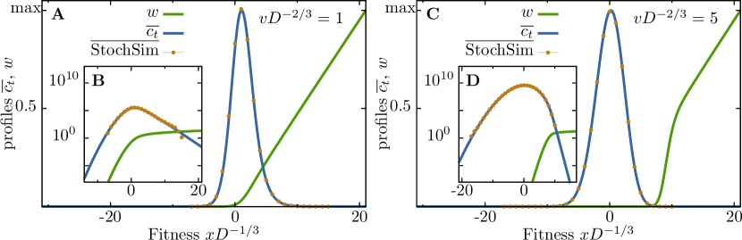
Figure 2: Numerical solution of the model of adaptation tuned to be closed at the first moment ($n=1$), and comparison with stochastic simulations. Averages from stochastic simulations (brown) coincide with numerical solutions of the mean stationary population density $\overline{c_{t}}$ (blue line) for small speeds (A, B) and large speeds (C, D), respectively. The weighting function $w(x,t)$ (green line) exhibits a sharp increase towards the nose of the wave, before crossing over to its asymptotic linear solution, $w(x,t)\approx x$, for large fitness. This is consistent with the interpretation of $u^{(n)}(x,t)=w(x,t)/(n+1)$ as fixation probability, tested in Fig. 4. Models tuned to be closed at higher moments ($n>1$) display the same features qualitatively and quantitatively, see Fig. 3.  

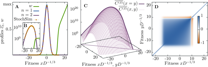
Figure 3: Numerical solution of the model of adaptation tuned to be closed at the second moment ($n=2$). A, B The mean population densities of the models with $n=2$ (purple) and $n=1$ (blue) for the same wave speed ( $vD^{-1/3}=6$) almost coincide. The profile for $n=2$ (and generally for larger $n$) is shifted to slightly larger fitness values, but the population size $\overline{N}$ is almost unaffected ($\overline{N}^{(n=1)}/\overline{N}^{(n=2)}-1\lesssim 0.02$), with even less deviations for larger population sizes (or adaptation speeds). Profiles from stochastic simulations subject to the constraint defined by $u^{(2)}$ are shown as brown dots. The standard error is smaller than the dot size. C The numerical solution of the second moment $\overline{C}^{(2)}(x,y)$ ($n=2$) is shown in a semi-logarithmic plot. The ridge $\overline{C}^{(2)}(x=y)$ is nearly parabolic except for its exponential tails. D From the second moment, we calculate the Pearson-product-moment-correlation $\rho(x,y)$ (see main text), which allows us to distinguish correlated (+1), uncorrelated (0) and anticorrelated (-1) variation. The nose of the wave clearly is anticorrelated with the bulk of the wave in our tuned models.

Model tuned to the first moment ($n=1$).

To set the stage and to reproduce earlier results from Ref. hallatschek2011noisy , we first present numerical results for the model closed at the first moment. Fig. 2 shows, for two wave speeds, the weighting function and the mean population density in a stationary comoving frame. While the population distribution is, except for an exponential decay in the wave-tip, close to a Gaussian for large speeds, it is markedly skewed for lower wave speeds. Note that the exact numerical results are in near perfect agreement with stochastic simulations, confirming our approach.

Model tuned to the second moment ($n=2$).

Fig. 2 characterizes the behavior of $n=2$ models in comparison with $n=1$ tuned models. Since $n=2$ models provide access to the second moment, one can of course also obtain the first, by contraction with the weighting function $u^{(n)}(x,t)$ (cf. Eq. (12)). Fig.  2B shows the mean population densities for both $n=1$ and $n=2$ models for the same velocity and weighting function $w$ which is identical to their respective weighting functions $u^{(1)}$ and $u^{(2)}$ up to an $n$–dependent factor, cf. Eq. (10). The mean population densities can hardly be distinguished in the figures - generally, the agreement of the two different models increases with increasing wave velocity or, equivalently, population size. Moreover, the stochastic simulations track the predicted mean in near perfect agreement, providing numerical support for our analysis of the tuned closure at higher moments.

Fig. 2B shows, in 3d plot, the second moment $\overline{C}^{(2)}(x,y)$ in a semi-logarithmic plot. While this plot is mostly Gaussian, it reveals a distinctly exponential decay in the front and back of the wave. This indicates the importance of fluctuations in these low-density regions.

Higher order correlation functions can also be used to directly investigate fluctuation properties of the noisy adaptation wave. The Pearson-product-moment-correlation, defined as $\rho(x,y)=\mathrm{Cov}[c_{t}(x),c_{t}(y)]/\sqrt{\mathrm{Var}[c_{t}(x)]\mathrm{Var}[c_{t}(y)]}$ shows a clear anticorrelation signal in the nose of the wave: Usually, a (stochastic) rise in population number in the nose of the wave leads to an overall decrease in population size. Such a very fit population has a much larger weight in the tuned constraint, Eq. (7), forcing the bulk population to be culled. Thus, bulk population size and nose population size are anticorrelated geyrhofer2015oscillations .

Fixation probabilities.

Note from Figs. 2 and 3 that the weighting functions $u^{(n)}(x,t)=2w(x,t)/b(n+1)$ strongly increase towards the tip of the wave where it crosses over to a linear increase. The functional form is consistent with the interpretation of a fixation probability: The success probability of an individual should be much larger in the tip of the wave rather than the bulk because it has to compete with less and less equally or more fit individuals. The fixation probability approaches a linear branch beyond some cross-over fitness because individuals there are so exceptionally fit that they merely have to survive random death to fix. The competition with conspecific is minimal - there is only competition with their own offspring.

To test our prediction that $u^{(n)}(x)$ can be interpreted, exactly, as an fixation probability, we have carried out the following test: We ran simulations for $n=1$ and $n=2$ tuned models, in which we labeled the tip of the wave such that the predicted fixation probability is exactly $50\%$, cf. Fig. 4. The measured fixation probability is shown in the insets of Fig. 4. Within the statistical error, the agreement is very good.

We would like to point out that the fact that $w(x,t)$ is strongly increasing towards the wave tip means that highly fit individuals have a large impact on what fraction of the population is culled per time step. For instance, if a single individual arises far out in the tail of the wave, it may have a large fixation probability. To keep the total fixation probability at one, this means that a significant fraction of the individuals need to be cleared from the population. Importantly, however, the culling itself is independent of the identity of individuals, i.e., a poorly fit individual is equally likely to die as a highly fit individual. This distinguishes our model from models that regularize the population size by removing cells preferentially at the wave tip. Such a procedure strongly modifies the wave dynamics and, in particular, reduces the amount of fluctuations.

Figure 4: Fixation in traveling wave models of adaptation sensitively depend on individuals in the nose of the wave. One of our key results is that tuned models generally have the convenient feature that fixation probabilities can be computed exactly – they are given by the tuned weighting function $u^{(n)}(x,t)=2w(x,t)/b(n+1)$. Here, we provide a test of this prediction. First, we have generated $50$ independent start configurations, and labeled the wave tip such that the labeled population is predicted to have a $50\%$ fixation probability, $\bigl{\langle}u^{(1)}|c_{\ell}\bigr{\rangle}=0.5$. Panel A shows one start configuration and the labeled subpopulation in orange. (The shown density profile (light blue area) is momentarily smaller than the mean density (blue line) due to random population size fluctuations, cf. Fig. 5). For each of the labeled start configurations, we ran $200$ simulations up until the (fixation) time where either the labelled subpopulation is extinct or has taken over. From counting the number of extinction and fixation events, Bayesian inference allows to compute the posterior distribution assuming a flat prior geyrhofer2014quantifying . B For the model with $n=1$, we find that $45$ of the $95\%$-confidence intervals of this Beta-distributed posterior include the expected fixation probability of $1/2$ (black intervals), while $5$ intervals scatter considerably due to lattice effects in simulations (red intervals). C When closing the moment hierarchy at $n=2$ results exhibit stronger scattering. However, the measured confidence intervals for $n=2$ reproduce the expected outcome to reasonable extent.

Velocity-Population-Size Relationships

Fig. 5 shows the relation between velocity and mean population size in various tuned models. As comparison, we also show the corresponding relationships between mean velocity and population size for fixed population size models. All these models correspond to different statistical ensembles, yet for large population sizes the curves approach each other very well.

The differences between models at finite population sizes is explained mainly by population size fluctuations: If we force the fixed population size model to fluctuate precisely as a given realization of a tuned model, we obtain very accurate agreement. Conversely, if we plot velocity vs. $\overline{\log N}$ shows excellent agreement between all models. This agreement is due to a timescale separation, discussed below.

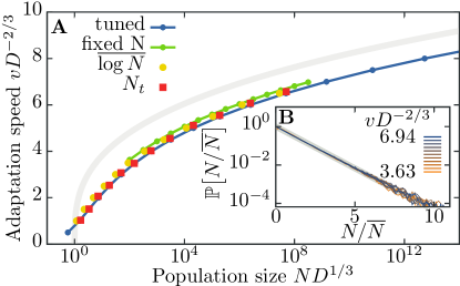
Figure 5: Fluctuations in adaption waves suggest the adaptation speed is controlled by the mean logarithmic population size. A Stochastic simulations reveal that, for a given speed of adaptation, tuned models have a larger mean population size $\overline{N}$ (blue line) than models of fixed population size (green line). The small discrepancy is much lower between these two models than to the best available cutoff theory (gray line cohen2005front ). Most of the remaining discrepancy is due to population size fluctuations (very nearly exponentially distributed, see inset B): When we measure fluctuations in a stochastic realization of the tuned model and impose exactly the same population size time series in repeated stochastic simulations, we obtain adaptation speed vs. mean population size relation that coincides with the one obtained for the tuned models (red circles). Importantly, fixed population size and tuned models have almost the same mean logarithmic population size, $\overline{\log N}$, for the same wave speeds. It can be shown that this is due to a time scale separation between slowly decaying population size fluctuations (coalescence time scale) and the fast relaxation of the wave speed (determined by a mixing time in the tip of the wave). Thus, the key dynamical quantity in traveling wave models with fluctuating population sizes is $\overline{\log N_{t}}$ instead of $\overline{N_{t}}$.

Decay of Genetic Diversity

Next, we have solved numerically for the mode spectrum that governs the decay of heterozygosity. Fig. 6 shows the behavior of the lowest two eigenvalues as a function of the velocity of the wave and the population size, respectively. It can be clearly seen that a time scale separation arises: The frequency of the first mode decays slowly to $0$, following $\tau_{c}\sim v$ to a good approximation. The frequency of the next higher mode, on the other hand, approaches a constant value of order $1/D$.

This means that coalescence takes much longer than the time until a subpopulation has forgotten its the initial condition of its spatial distribution. This time-scale separation not only helps in analytically finding the coalescence time in Sec. VI.2.2. But it also underlies the ensuing Bolthausen-Sznitman coalescence in many models of adaptation and invasion waves of the Fisher-Kolmogorov type desai2013genetic ; neher2013genealogies .

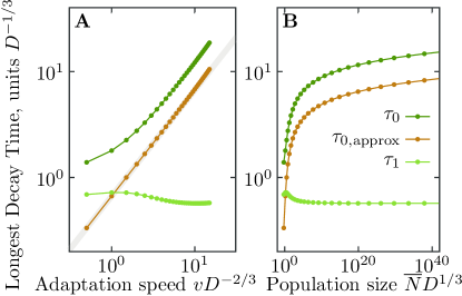
Figure 6: Time scales for the decay of genetic diversity in models of adaptation. In models with limited population size, the ultimate fate of a subpopulation of neutral mutants is to either go extinct or to fixation. Hence, the diversity of the population will gradually decay unless new mutations come in, and quantifying this decay is an important population genetic challenge. This figure quantifies the leading decay times of the function $\overline{C}^{(2)}_{1,2}$ correlating the densities of labeled and unlabeled individuals. The decay times were found from a spectral analysis of the equation of motion of $\overline{C}^{(n)}_{1,2}$, which is linear in the model tuned to be closed at the level of two-point correlation functions ($n=2$). A Our numerical results suggest that, for the considered model with diffusion kernel, the slowest decay time approaches $\tau^{(n=2)}_{0}\propto v\sim\bigl{(}\ln N\bigr{)}^{1/3}$ for large speeds (gray line indicates $\bigl{(}\ln N\bigr{)}^{1/3}$). By contrast, the second slowest decay time $\tau^{(n=2)}_{1}$ approaches a constant for large populations. This indicates an important time scale separation, as we argue in the main text. Also note that the numerical results approach, for large $N$, the approximation $\tau_{0,\,\mathrm{approx}}$ in Eq. (47), which is based on the time scale separation of the two lowest eigenvalues emerging for large population sizes. Panel B shows the same quantities as Panel A as a function of the population size $\overline{N}$.

Invasion waves

After changing the Liouville operator the one in Eq. (8), and following the same numerical pipeline as described above, we obtain analogous results for invasion waves, see Fig. (7). Note that the spatial co-ordinate now corresponds to real space rather than a fitness landscape. Our data reproduce the universal velocity-population size relationship and the coalescence time scaling that have been established for FKPP waves over the last 20 years van2003front ; brunet2006phenomenological . An explicit form of the equations we solved numerically can be found in Appendix A.

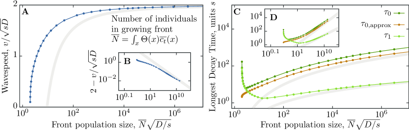
Figure 7: Invasion waves. Here, we summarize our numerical results for models of invasion tuned to be closed at the second moment, $n=2$. A Wave speed as a function of population size. The inset B compares our results with the leading order cut-off correction $v\sqrt{Dr}-2\sim\pi^{2}/(\ln\overline{N})^{2}$. C shows the two longest decay times, $\tau_{0}>\tau_{1}$, of the second moment. The increasing gap between both decay times manifests a time scale separation. The double logarithmic plot in inset D shows that the longest decay time follows $\tau_{0}\sim\ln N^{3}$ (upper gray lines) asymptotically and, hence, behaves as the predicted coalescence time in FKPP waves brunet2006phenomenological . By contrast, the second decay time follows $\tau_{1}\sim\ln N^{2}$ (lower gray line).

V The Stochastic Dynamics of Branching Random Walks

In the following we proceed with the derivation of our main results quoted above. To this end, we will first recapitulate the derivation of the stochastic differential equation governing the dynamics of branching random walks, as was done in Ref. hallatschek2011noisy . We will then discuss the consequences of this stochastic dynamics for $n$-point correlation functions, which will allow us to identify the natural choice of the weighting function $u^{(n)}$. Subsequently, we will discuss how to modify our basic model to account for different subtypes within the population.

V.1 Stochastic dynamics of Constrained Branching Random Walks

We will now determine the stochastic dynamics obtained in the limit $\epsilon\to 0$, which is in general non-linear and hence not solvable. We then use the ensuing stochastic differential equation to identify special models with closed moment hierarchies. We will find that these tuned models are not only solvable, but also allow for a natural interpretation of the constraint in terms of fixation probabilities.

The stochastic dynamics of a constrained branching random walk (CBRW) was derived in Ref. hallatschek2011noisy and may be summarized as follows. The state of the system is described by the number density $c_{t}(x)$ of random walkers at position $x$ and time $t$. At any time, the distribution of random walkers has to satisfy a global constraint defined by Eq. (7).

The combination of Eqs. (1) and (7) can be written as a fraction,

$$c_{t+\epsilon} = \frac{c_{t}+\epsilon\mathcal{L}c_{t}+\sqrt{\epsilon bc_{t}}\eta_{t}}{\bigl{\langle}u_{t+\epsilon}|c_{t}+\epsilon\mathcal{L}c_{t}+\sqrt{\epsilon bc_{t}}\eta_{t}\bigr{\rangle}}\;,$$ (17)

in the continuous-time limit (small enough $\epsilon$ is required to ensure that the denominator of the fraction is never far from $1$). Note that the expression in Eq. (17) evidently satisfies the constraint, $\langle u_{t+\epsilon}|c_{t+\epsilon}\rangle=1.$

Moreover, in the continuous-time limit, we only need to retain terms up to order $O(\epsilon)$ van1992stochastic . Thus, expanding Eq. (17), we obtain

$$c_{t+\epsilon} = c_{t}+\sqrt{\epsilon}\left[\sqrt{bc_{t}}\eta_{t}-c_{t}\bigl{\langle}u_{t}|\sqrt{bc_{t}}\eta_{t}\bigr{\rangle}\right]$$ (18)

$$~{}~{}+\epsilon\left[\mathcal{L}c_{t}-\sqrt{bc_{t}}\eta_{t}\bigl{\langle}u_{t}|\sqrt{bc_{t}}\eta_{t}\bigr{\rangle}-c_{t}\bigl{\langle}\partial_{t}u_{t}|c_{t}\bigr{\rangle}-c_{t}\bigl{\langle}u_{t}|\mathcal{L}c_{t}\bigr{\rangle}+c_{t}\bigl{\langle}u_{t}|\sqrt{bc_{t}}\eta_{t}\bigr{\rangle}^{2}\right]\;.$$

In Eq. (18), we required $u_{t}$ to change only deterministically, $u_{t+\epsilon}=u_{t}+\epsilon\partial_{t}u_{t}+o(\epsilon)$, i.e. it has no stochastic component.

Finally, we replace products of order $\eta_{t}\eta_{t^{\prime}}$ in the deterministic term of expansion Eq. (18) with their averages, Eq. (4) , to arrive at the following stochastic differential equation: The temporal change $\Delta c_{t}\equiv c_{t+\epsilon}-c_{t}$ of the concentration field $c_{t}$ from time $t$ to $t+\epsilon$ can be written as

$$\Delta c_{t}(x)\equiv c_{t+\epsilon}-c_{t}=\epsilon\Delta^{(d)}c_{t}(x)+\sqrt{\epsilon}\Delta^{(s)}c_{t}(x)\;,$$ (19)

which consists of a deterministic change $\epsilon\Delta^{(d)}c_{t}$ of order $O(\epsilon)$ and a stochastic change $\sqrt{\epsilon}\Delta^{(s)}c_{t}$ of order $O(\epsilon^{1/2})$. These are given by

$$\Delta^{(d)}c_{t}(x) = \left(\mathcal{L}_{t}-bu_{t}\right)c_{t}-\bigl{\langle}\bigl{(}\partial_{t}+\mathcal{L}_{t}^{\dagger}-bu_{t}\bigr{)}u_{t}\mid c_{t}\bigr{\rangle}c_{t}\;,$$

$$\Delta^{(s)}c_{t}(x) = \eta_{t}\sqrt{bc_{t}}-\bigl{\langle}u_{t}\mid\eta_{t}\sqrt{bc_{t}}\bigr{\rangle}c_{t}\;.$$ (20)

Thus, we have arrived at the continuous-time stochastic process for a constrained branching random walk hallatschek2011noisy , which summarizes the combined effect of the original two-step algorithm, (i) “branching random walk” and “enforce constraint”. The related concept of forcing the solution of a SDE onto a manifold has been analyzed in katzenberger1991solutions .

V.2 Moment equations

This section introduces the hierarchy of moment equations of CBRWs that characterize the mean and the fluctuations of the concentration field of the random walkers.

Consider the dynamics of the products of $C^{(n)}_{t}$. Our goal is to determine how the function $C^{(n)}_{t}$ changes as time marches forward. To this end, we express the time increments of the $n$–point products $C^{(n)}_{t}$ in terms of the changes of the single fields $c_{t}$,

$$C^{(n)}_{t+\epsilon}=\prod_{j=1}^{n}c_{t+\epsilon}(x_{j})=\prod_{j=1}^{n}\left[c_{t}(x_{j})+\epsilon\Delta^{(d)}c_{t}(x_{j})+\sqrt{\epsilon}\Delta^{(s)}c_{t}(x_{j})\right]\;,$$ (21)

using the deterministic and stochastic time increments $\Delta^{(d/s)}c$ computed in (V.1). Next, we expand the product up to order $O(\epsilon)$,

$$\Delta C^{(n)}_{t} = \sqrt{\epsilon}\sum_{j=1}^{n}C_{t}^{(n-1)}(\backslash x_{j})\Delta^{(s)}c_{t}(x_{j})$$

$$+\epsilon\left[\sum_{j=1}^{n}C_{t}^{(n-1)}(\backslash x_{j})\Delta^{(d)}c_{t}(x_{j})+\sum_{j=1}^{n-1}\sum_{k=j+1}^{n}C_{t}^{(n-2)}(\backslash x_{j},\backslash x_{k})\Delta^{(s)}c_{t}(x_{j})\Delta^{(s)}c_{t}(x_{k})\right]\;.$$

Note that the last term arises only for $n\geq 2$. Inserting the time increments Eq. (V.1) of the single fields into Eq. (V.2) yields

$$\Delta C^{(n)}_{t} = \sqrt{\epsilon}\left[\sum^{n}_{j=1}\sqrt{bc_{t}(x_{j})}\eta_{t}(x_{j})C_{t}^{(n-1)}(\backslash x_{j})-n\bigl{\langle}u_{t}\mid\eta_{t}\sqrt{bc_{t}}\bigr{\rangle}C_{t}^{(n)}\right]$$

$$+\epsilon\left[\sum^{n}_{j=1}\left.\left(\mathcal{L}-bu_{t}\right)\right|_{x_{j}}C^{(n)}_{t}-n\bigl{\langle}\left(\partial_{t}+\mathcal{L}^{\dagger}-bu_{t}\right)u_{t}\mid c_{t}\bigr{\rangle}C_{t}^{(n)}\right]$$

$$+\epsilon\sum_{j=1}^{n-1}\sum_{k=j+1}^{n}b\sqrt{c_{t}(x_{j})c_{t}(x_{k})}\eta_{t}(x_{j})\eta_{t}(x_{k})C^{(n-2)}_{t}(\backslash x_{j},\backslash x_{k})$$

$$-\epsilon(n-1)\sum^{n}_{j=1}\sqrt{bc_{t}(x_{j})}\eta_{t}(x_{j})\bigl{\langle}u_{t}\mid\eta_{t}\sqrt{bc_{t}}\bigr{\rangle}C^{(n-1)}_{t}(\backslash x_{j})$$

$$+\epsilon\frac{n(n-1)}{2}\bigl{\langle}u_{t}\mid\eta_{t}\sqrt{bc_{t}}\bigr{\rangle}^{2}C^{(n)}_{t}\;.$$

Within the deterministic $O(\epsilon)$ terms, we again replace products of noises in terms of their averages, as given by Eq. (4). We then obtain

$$\Delta C^{(n)}_{t} = \sqrt{\epsilon}\left[\sum^{n}_{j=1}C_{t}^{(n-1)}(\backslash x_{j})\sqrt{bc_{t}(x_{j})}\eta_{t}(x_{j})-nC_{t}^{(n)}\langle u\mid\eta_{t}\sqrt{bc_{t}}\rangle\right]$$ (24)

$$+\epsilon\left[\sum^{n}_{j=1}\left.\left(\mathcal{L}-bnu_{t}\right)\right|_{x_{j}}C^{(n)}_{t}+b\sum_{j=1}^{n}\sum_{k=j+1}^{n}\delta(x_{j}-x_{k})C^{(n-1)}_{t}(\backslash x_{k})\right]$$

$$-\epsilon n\left\langle\left(\partial_{t}+\mathcal{L}^{\dagger}-b(n+1)/2\,u_{t}\right)u_{t}\mid c_{t}\right\rangle C^{(n)}_{t}\;.$$

Upon averaging and sending $\epsilon$ to zero, we obtain an equation of moment for the $n$th moment,

$$\partial_{t}\overline{C}^{(n)}_{t}=\sum^{n}_{j=1}\left.\left(\mathcal{L}-bnu_{t}\right)\right|_{x_{j}}\overline{C}^{(n)}_{t}+b\sum_{j=1}^{n}\sum_{k=j+1}^{n}\delta(x_{j}-x_{k})\overline{C}^{(n-1)}_{t}(\backslash x_{k})-n\bigl{\langle}\left(\partial_{t}+\mathcal{L}^{\dagger}-b(n+1)/2\,u_{t}\right)u_{t}\mid\overline{C}^{(n+1)}_{t}\bigr{\rangle}_{x_{n+1}}\;.$$ (25)

From (25) we observe that the coupling to higher moments $\overline{C}^{(n+1)}_{t}$ is mediated via the dynamics of the weighting function $u_{t}$ in the last term.

V.3 Exact closure

The key result of Ref. hallatschek2011noisy was that a particular choice of the weighting function $u_{t}$ exists, for which the first moment equation is closed. We now show that exact closures can be found for higher moments as well.

Suppose, the solution $u^{(n)}_{t}(x)$ of

$$-\partial_{t}u_{t}^{(n)}=\left[\mathcal{L}^{\dagger}-\frac{b(n+1)}{2}u_{t}^{(n)}\right]u_{t}^{(n)}$$ (26)

exists, and we choose $u_{t}^{(n)}$ as the weighting function. For this particular model, the dependence on the $(n+1)$th moment in Eq. (25) disappears identically:

$$\partial_{t}\overline{C}^{(n)}_{t}=\sum^{n}_{j=1}\left.\left(\mathcal{L}-bnu^{(n)}_{t}\right)\right|_{x_{j}}\overline{C}^{(n)}_{t}+b\sum_{j=1}^{n}\sum_{k=j+1}^{n}\delta(x_{j}-x_{k})\overline{C}^{(n-1)}_{t}(\backslash x_{k})\;.$$ (27)

Thus, the hierarchy of the first $n$ moments is closed. In fact, this closed set of $n$ differential equations can be summarized by a single integro-differential equation, Eq. (12), because contracting $\overline{C}^{(n)}_{t}$ with $u^{(n)}$ reduces the order of the moments by virtue of the constraint, cf. Eq. (16).

The final form of our results Eq.s (11), (12) are obtained upon substituting

$$u_{t}^{(n)}(x)=\frac{2w(x;t)}{b(n+1)}\;,$$ (28)

which is the initially quoted Eq. (10).

In summary, starting from a linear operator $\mathcal{L}$, we have identified an algorithm to construct a constrained branching walk model solvable up to the $n$th moment: First, identify the weighting function $w(x,t)$ for which the hierarchy of moment equation closes at the $n$th moment. To this end, solve equation (26), which is deterministic nonlinear equation for the weighting function $w(x,t)$ depending on a space and a time variable. Second, solve the corresponding moment equation (12), which is a linear equation for the function $\overline{C}^{(n)}$ that depends on $n$ space variables and a time variable. Once the function $\overline{C}^{(n)}$ has been obtained, any lower-order moment follows by contraction with $u^{(n)}\propto w$, as described in Eq. (16).

VI Accounting for different subtypes

We now extend our model to account for $k$ different types of individuals. This enables studying questions such as how does mutator strain take over in an evolving population of bacteria even if it confers a direct fitness detriment, or, how does a faster dispersing mutant spreads during a growing tumor even if it might be slower growing? Moreover, we can discuss the decay of genetic diversity and arrive at the very important conclusion that $w(x,t)$ is always the fixation probability of a neutral mutation arising at position $x$ and time $t$ by considering exchangeable subtypes.

To this end, we define the dynamics of the subtypes analogously to our original constrained branching walk model for the total population in Sec. V: The number density of individuals of type $i$ at position $x$ at time $t$ shall be given by a density field $c_{i}(x,t)$. Hence, the entire state of the system is described by the vector $\vec{c}(x,t)=\{c_{i}(x,t)\}_{i\in\{1,k\}}$. In each time step, a given subtype undergoes a step of branching random walk subject to their own linear dynamics encoded by an operator $\mathcal{L}_{i}$ and their own fluctuations generated by a noise field $\eta_{i}(x,t)$,

$$\tilde{c}_{i}(t+\epsilon)-c_{i}(t)=\epsilon\mathcal{L}_{i}c_{i}+\sqrt{\epsilon b_{i}c_{i}}\,\eta_{i}\;.$$ (29)

The $i$–dependence of the linear operators $\mathcal{L}_{i}$ encode the phenotypic differences between types. E.g. if type $i$ would refer to a mutator type, $\mathcal{L}_{i}$ would include a particular mutational operator $\mathcal{M}_{i}$ characterizing the mutator phenotype. For instance, if mutations are modeled by diffusion, the corresponding diffusion constant of a mutator would be larger than that of the wild type.

The different subtypes are coupled only by the second computational substep

$$c_{i}(x,t+\epsilon)=\tilde{c}_{i}(x,t+\epsilon)(1-\lambda)\;,$$ (30)

which ensures a global constrained defined by a weighting function vector $\vec{u}=\{u_{i}\}_{i}$,

$$1=\int_{x}\sum_{i}u_{i}(x,t)c_{i}(x,t)\equiv\langle\vec{u}\mid\vec{c}\rangle\;.$$ (31)

Notice that we have merely added another (discrete) dimension to the problem - the type degree of freedoms. It may be checked that our arguments to arrive at an effective stochastic differential equation and for closing the moment hierarchy in Sec. generalize to any number of dimensions. Thus, we can immediately restate our central results for the extended model accounting for sub-types.

In particular, if we choose the weighting function vector to be $u^{(n)}_{i}=2w_{i}/b_{i}(n+1)$ with

$$\partial_{t}w_{i}(x,t)=\left[\mathcal{L}_{i}-w_{i}(x,t)\right]w_{i}(x,t)\;,$$ (32)

then equation of motion for the $n^{\text{\tiny th}}$ moment will be closed. If we choose the notation

$$C^{(n)}_{i_{1},...,i_{n}}(x_{1},\dots,x_{n};t)\equiv\prod_{j=1}^{n}c_{i_{j}}(x_{j},t)\;,$$ (33)

with $i_{j}$ being the type of the $j^{\text{th}}$ number density field in the product on the right-hand-side. The equation of motion for the $n^{\text{\tiny th}}$ moment is given by

$$\partial_{t}\overline{C}^{(n)}_{i_{1},...,i_{n}}(x_{1},\dots,x_{n};t)=\sum^{n}_{j=1}\left.\left(\mathcal{L}_{i_{j}}+\gamma(t)-\frac{2n}{n+1}w_{i_{j}}\right)\right|_{x_{j}}\overline{C}^{(n)}_{i_{1},...,i_{n}}+\frac{2}{n+1}\sum_{j=1}^{n}\sum_{k=j+1}^{n}\delta_{i_{j},i_{k}}\delta(x_{j}-x_{k})\left\langle\vec{w}\mid\overline{C}^{(n)}_{i_{1},...,i_{n}}\right\rangle_{k}\;.$$ (34)

Notice that the correlations indicated by the last term only arise for a subpopulation with itself, $i_{j}=i_{k}$.

VI.1 The neutral case and interpretation of the weighting function

Now, let us focus on the special case where types follow the same dynamics in the statistical sense,

$$\mathcal{L}_{i}=\mathcal{L}\;,\qquad w_{i}(x,t)=w(x,t)\;,\qquad b_{i}=b\;.$$ (35)

For such “exchangeable” subtypes, it is easy to see that the equation of motion Eq. (12) for the $n^{\text{\tiny th}}$ moment of the total population, $c(x,t)=\sum_{i}c_{i}(x,t)$, is obtained upon summing left and right-hand side of Eq. (34) over all type indices, i.e. by carrying out $\sum_{i_{1}}\sum_{i_{2}}...\sum_{i_{n}}$.

We can single out one particular subpopulation, say $i_{1}=\ell$ ($\ell$ for labeled), by summing the equation of motion over all other type indices, $\sum_{i_{2}}...\sum_{i_{n}}$. This yields

$$\partial_{t}\overline{c_{\ell}(x_{1};t)C^{(n-1)}(x_{2},\dots,x_{n};t)} = \sum^{n}_{j=1}\left.\left(\mathcal{L}+\gamma(t)-\frac{2n}{n+1}w\right)\right|_{x_{j}}\overline{c_{\ell}(x_{1};t)C^{(n-1)}(x_{2},\dots,x_{n};t)}$$ (36)

$$+ \frac{2}{n+1}\sum_{j=1}^{n}\sum_{k=j+1}^{n}\delta(x_{j}-x_{k})\left\langle w\mid\overline{c_{\ell}(x_{1};t)C^{(n-1)}(x_{2},\dots,x_{n};t)}\right\rangle_{k}\;.$$ (37)

Note that the correlation function $\overline{c_{\ell}C^{(n-1)}}$ satisfies the same linear equation as $\overline{C}^{(n)}$ does Eq. (12), which we abbreviate as

$$\partial_{t}\overline{c_{\ell}(x_{1};t)C^{(n-1)}(x_{2},\dots,x_{n};t)} = \mathcal{G}\overline{c_{\ell}C^{(n-1)}}$$ (38)

$$\partial_{t}\overline{C}^{(n)}(x_{1},\dots,x_{n};t) = \mathcal{G}\overline{C}^{(n)}\;.$$ (39)

defining a linear (integro-differential) operator $\mathcal{G}$. Imagine solving for the left eigenvector of $\mathcal{G}$ corresponding to eigenvalue 0,

$$0=\mathcal{G}^{\dagger}M^{(n)}$$ (40)

where $M^{(n)}(x_{1},...,x_{n})$ is a function of $n$ variables just like $C^{(n)}$. Then, contracting Eq. (36) with this new function one obtains

$$\langle M^{(n)}|\overline{c_{\ell}C^{(n-1)}}\rangle=\text{const.}=p^{\text{fix}}\langle M^{(n)}|\overline{C}^{(n)}\rangle\;.$$ (41)

The second equality is a key step. It holds because $c_{\ell}C^{(n-1)}\to C^{(n)}$ on long times if fixation occurs and $c_{\ell}C^{(n-1)}\to 0$, otherwise.

Hence, the fixation probability $p_{\ell}^{\text{fix}}$ of the labeled subpopulation with initial density $c_{\ell,0}(x)$ at time $0$ is given by

$$p_{\ell}^{\text{fix}}=\frac{\langle M^{(n)}|\overline{c_{\ell}C^{(n-1)}}\rangle}{\langle M^{(n)}|\overline{C}^{(n)}\rangle}\;.$$ (42)

Fortunately, the left eigenvector of $\mathcal{G}$ is easily constructed: If we fully contract Eq. (39) with $n$ factors of the weighting function $u^{(n)}(x_{i})$, we have to get $0$ on the LHS because of the constraint Eq. (7). Hence, the sought-after left eigenvector can be written as

$$\bigl{\langle}M^{(n)}|\overline{C}^{(n)}\bigr{\rangle}=\left(\prod_{i}\int_{x_{i}}u^{(n)}(x_{i})\right)\overline{C}^{(n)}(x_{1},\dots,x_{n})\;,$$ (43)

Since this eigenvectors contracts to 1 with the total population, Eq. (42) becomes

$$p_{\ell}^{\text{fix}}=\bigl{\langle}u^{(n)}|c_{\ell,0}\bigr{\rangle}=\frac{2\int dx\,w(x)c_{\ell,0}(x)}{b(n+1)}\;,$$ (44)

Thus, as announced in Section III, a single labeled mutant at a certain location $x$ has probability $u^{(n)}(x)$ that its descendants will take over the population on long times.

VI.2 Decay of heterozygosity

The diversity of labels in a population will inevitably decline, because of the rise and ultimate fixation of one of the labels initially present. One can capture the gradual loss of genetic diversity by studying the expectation of the product of density fields that correspond to different types. For instance, if there are just two types, $i\in\{1,2\}$, the correlation function $\overline{C}^{(2)}_{12}(x,y;t)=\overline{c_{1}(x,t)c_{2}(y,t)}$ satisfies

$$\partial_{t}\overline{C}^{(2)}_{12}(x,y;t)=\sum^{n=2}_{j=1}\left.\left(\mathcal{L}+\gamma(t)-\frac{2n}{n+1}w\right)\right|_{j}\overline{C}^{(2)}_{12}\;.$$ (45)

Notice that the right-hand side of Eq. (45) misses the positive $\delta$–function term of Eq. (12), which characterized the $n^{\text{\tiny th}}$ moment of the total population density. Assuming that $\overline{C}^{(2)}$ (as well as $\overline{C}^{(2)}_{1,1}$ and $\overline{C}^{(2)}_{2,2}$) have a stable stationary solution, we can conclude that $\overline{C}^{(2)}_{1,2}$ will decay to $0$ at long times because of the lacking source term. This is to be expected because the gradual fixation of one of the two types implies that $\overline{C}^{(2)}_{1,2}$ has to approach $0$ on long times. Discerning relaxation times of the time-evolution (45) is related to a key question in population genetics: How fast do lineages of two individuals coalesce?

The function $C^{(2)}_{1,2}$ is closely related to the so-called heterozygosity in population genetics. The heterozygosity in the population is the probability that two randomly chosen individuals are of different type, $H(t)=\int_{x}\int_{y}\overline{C^{2}_{1,2}(x,y;t)/N^{2}(t)}$. For our purposes, it is much more convenient and natural to consider a variant of that quantity,

$$\hat{H}(t)=\int_{x}\int_{y}u^{(n)}(x,t)u^{(n)}(y,t)C^{2}_{1,2}(x,y;t)=\langle u^{(n)}|c_{1}\rangle\langle u^{(n)}|c_{2}\rangle=p(t)q(t)$$ (46)

with $p(t)\equiv\langle u^{(n)}|c_{1}\rangle$ and $q(t)\equiv\langle u^{(n)}|c_{2}\rangle$. These quantities have nice properties. At any time, both $p(t)$ and $q(t)$ represent the probability of fixation of the respective subpopulations. Accordingly, we have $p(t)+q(t)=1$, ensured by the global constraint. Thus, $\hat{H}(t)$ is similar to a heterozygosity in neutral populations and, under certain conditions discussed below, even converges against the actual heterozygosity.

An equation of motion for the expectation $\overline{\hat{H}(t)}$ can be derived by contracting Eq. (45) twice with $u^{(n)}$ and using the equation of motion of $u^{(n)}$, Eq. (11),

$$\partial_{t}\overline{\hat{H}(t)}=-\frac{n-1}{(n+1)^{2}}\left(\overline{p(t)\left\langle w^{2}|c_{2}\right\rangle}+\overline{q(t)\left\langle w^{2}|c_{1}\right\rangle}\right)\;.$$ (47)

Notice that the right-hand side is negative always. Thus, again, we see that the heterozygosity will necessarily decay.

VI.2.1 Separation ansatz

As in Eq. (45) for $n=2$, one can easily see that the equation of motion for $\overline{C}^{(n)}_{i_{1},\cdots,i_{n}}$ is separable for the $n$ components if $i_{j}\neq i_{k}$. It therefore admits a solution of the simple form

$$C^{(n)}_{i_{1},\cdots,i_{n}}=\prod_{k=1}^{n}f_{i_{k}}(x_{i_{k}};t)$$ (48)

with $f_{i_{k}}(x_{i_{k}};t)$ satisfying a one-dimensional linear equation

$$\partial_{t}f_{i_{k}}(x;t)=\left(\mathcal{L}+\gamma(t)-\frac{2n}{n+1}w\right)f_{i_{k}}(x;t)$$ (49)

subject to the initial conditions $f_{i_{k}}(x;0)=c_{i_{k}}(x;0)$. By contracting with $w$ and using its dynamics, $-\partial_{t}w=\bigl{(}\mathcal{L}^{\dagger}-w\bigr{)}w$,

$$\partial_{t}\langle w|f_{i_{k}}\rangle=-\frac{n-1}{n+1}\langle w^{2}|f_{i_{k}}\rangle\;,$$ (50)

we see that $f(x;t)$ must be continuously decaying with time.

On long times, we can assume that $f(x,t)\sim a(t)\psi(x)$, where $\psi(x)$ is the eigenfunction to the largest eigenvalue of Eq. (49). Inserting this asymptotic behavior into Eq. (50) yields an exponential decay $\partial_{t}a=-a/\tau_{c}$ of the mode amplitude $a(t)$ with a decay time given by

$$\tau_{c}=\frac{n+1}{n-1}\frac{\langle w|\psi\rangle}{\langle w^{2}|\psi\rangle}\;,$$ (51)

Intuitively, this decay time describes how long it takes until significant fraction of the population has coalesced. Thus, one expects $\tau_{c}$ to depend on the fundamental parameters of the considered model in just the same way as the population coalescence time. The numerical coefficient, of course, will be different by a factor of order 1.

Due to the one-dimensional nature of Eq. (48), it is possible to obtain good approximations to the longest relaxation time for various models, either by directly solving the eigenvalue problem or by guessing the function $\psi$ in Eq. (51). We will provide a heuristic calculation for the case of a diffusive kernel in the limit of large populations (or fast waves).

VI.2.2 Time-scale separation

In most models of noisy traveling waves, one has found empirically a time scale separation: For large $\ln N$, the longest relaxation time of the mean density field is much shorter than the coalescence time. In the case of adaptation waves and invasion waves with diffusion kernel, this is evident from gap in the two lowest relaxation times in our numerical results in Fig. 6, 7B (also see SI Fig. 8).

In the presence of such a time-scale separation, we can approximate $c_{1}(x,t)\approx p(t)\overline{c}(x,t)$ and $c_{2}(x,t)\approx q(t)\overline{c}(x,t)$. For the purpose of using these approximations in the terms involving $\langle w^{2}|c_{i}\rangle$ in Eq. 47, we need them to be good in the high fitness tail. Then, we obtain

$$\partial_{t}\overline{\hat{H}(t)}\approx-2\frac{n-1}{(n+1)^{2}}\overline{p(t)q(t)}\left\langle w^{2}|\overline{c}\right\rangle\;,$$ (52)

suggesting that the time scale for coalescence scales as

$$\tau_{0,\,\mathrm{approx}}\propto\left\langle w^{2}|\overline{c}\right\rangle^{-1}\;.$$ (53)

This approximation indeed seems to approach the correct time scale for large $\ln N$, as can be appreciated from Figs. 6 and 7B.

VII Discussion

The ecological and evolutionary fate of populations often depends on a small number of “pioneers”, distinguished by their growth rates, migration rates, location, or other characteristics correlated with long-term survival. Most analyses of these inherently stochastic problems have focussed on the mean behavior of the population, which sensitively depends on fluctuations in the pioneer populations. Yet, the mean behavior says little about any given realization, the variability between realizations and their correlation times.

Here, we have shown that fluctuations can be analyzed in principle, if one relies on minimal models that reduce the dynamics to two essential ingredients: (1) Birth, death and jumps give rise, effectively, to a branching random walk. (2) A non-linear population regulation makes sure that those branching processes do not get out of control. For such constrained branching random walks, we have provided a general route towards analyzing fluctuations. The basic idea of the method is to adjust the population control, an essential non-linearity, in such a way that the equations describing correlation functions of order $n$ are closed.

Our method can be used to elucidate variability between replicates in evolution experiments as well as the genetic diversity within a population. To provide specific results, we have focussed on simple models of adaptation and of invasions. In both cases, we have found that the decay of genetic diversity scales as a power of the logarithm of the population size for large population sizes. Higher moments show a marked anticorrelation between the dynamics in the tip and the bulk of the wave. Moreover, we found that, for the models analyzed, the time scale for the decay of higher order correlations, such as the genetic heterozygosity, is much longer than the time the population wave needs to equilibrate at a given speed or population size. The presence of such a time scale separation simplifies the analysis of coalescence times considerably.

The ensemble of the resulting tuned models is complementary to established models of adaptation. While the latter have fixed population and fluctuating speeds of adaptation, the former has a fluctuating population size but fixed wave speeds. The resemblance of both ensembles relies on the fact that the fluctuations occur on time scales long compared to the relaxation time of the population wave. Quantities that only depend on the mean logarithm of the population size, such as the wave speed or the coalescence time, thus agree asymptotically in both ensembles, see e.g. Fig. 5, 7.

One might wonder about the net-effect of noise on models of adaptation and other traveling waves. If one is only concerned with the mean, many previous works have assumed that the effect of noise can be summarized by an effective cutoff in the tip of the wave tsimring1996rna ; brunet1997shift ; cohen2005front . This cutoff effect can be explicitly seen in the closed first moment equation of tuned models, as was already pointed out in Ref. hallatschek2011noisy . However, what is the effect of noise on higher-order correlations? Our general formulation in Eq. (12) of the $n^{\text{\tiny th}}$ moment exhibits, in general, two terms with different signs that are unexpected in a deterministic framework. One term tends to generate positive correlations between nearby individuals (in fitness space). These correlations then dissipate over distances due to the term with negative sign. Importantly, the correlation term becomes dominating in the tip of the wave due to its density dependence. The net-effect of fluctuations on the correlations emphasizes the complex nature of fluctuations, which only to the lowest order can be captured by a simple cutoff term in an effective Liouville operator.

The branching random walk contains a parameter $b$, the variance in offspring numbers per generation, that effectively measures the strength of genetic drift. Surprisingly, the noise-induced terms do not depend on this parameter $b$. This means that the noise-induced terms are not small, in general, even if the parameter $b$ is small, such that a controlled small-noise perturbation analysis is not possible. This reinforces the observation that noise is a singular perturbation that fundamentally impacts the outcome of ecological and evolutionary processes.

Our method of model tuning is quite versatile as it applies to any branching random walk subject to a global constraint. This includes models that combine ecology and evolution barton2013modelling ; pelletier2009eco or epistatic models in which mutations are not simply additive but might interact tenaillon2014utility . However, for more complex scenarios of interest to evolutionary biologists, one would like to introduce additional non-linearities. For instance, sex and recombination is a quadratic non-linearity as it depends on the the probability density of two different individuals finding each other and mating neher2010rate . In evolutionary game theory, one is interested in mutants that have a frequency-dependent advantage reiter2014range ; kussell2014non . The fitness of producers of a common good depends on the frequency of producers. This, again, introduces a non-linearity, which is quadratic in the simplest case.

Such non-linearities cannot be included in an exact way because they generate higher-order terms. However, it may be a useful approach to build them in and truncate the moment hierarchy at an appropriate order provided one can show that the neglected terms really are small. We believe that such reasoning should work, typically, if the non-linearities do not strongly influence the dynamics in the small density regions where the noise strength is large. A truncation scheme would, in this case, amount to matching a stochastic but linear description of the wave tip with a deterministic but non-linear bulk of the wave. We would welcome future work to examine these possibilities.

VIII Acknowledgments

Thanks to Peter Pfaffelhuber for useful discussions and making us aware of Ref. katzenberger1991solutions . This work was partially supported by a Simons Investigator award from the Simons Foundation (O.H.), the Deutsche Forschungsgemeinschaft via Grant HA 5163/2-1 (O.H.).

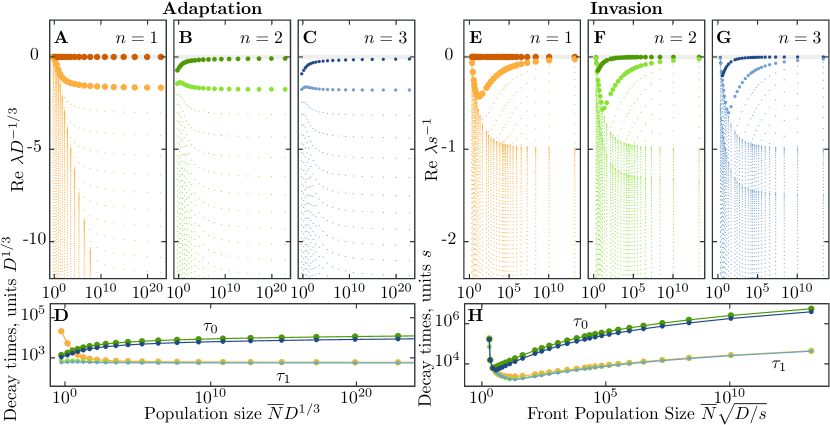
Figure 8: Relaxation rate spectra for models of adaptation and invasion. This figure quantifies the relaxation rates of correlations among labeled subpopulations in models of adaptation (left) and invasion (right). The relaxation rates $\lambda_{i}$ for the $n^{\text{\tiny th}}$ model were found from a spectral analysis of the equation of motion for $n$ separable subpopulations in the $n^{\text{\tiny th}}$ correlation function, cf. Eq. (49). All eigenvalues are real and negative, i.e., they lead to the decay of correlations. Each relaxation rate $\lambda_{i}$ corresponds to a relaxation time $\tau_{i}=1/\lambda_{i}$. D and F show the behavior of the two slowest decay rates $\tau_{0}$ and $\tau_{1}$ together with an approximation for $\tau_{0}$. The ratio $\tau_{0}/\tau_{1}$ controls the time scale separation between coalescence (slow) and wave profile relaxation (fast). In addition, the effects of chosing a particular $n$ for the closure of the moment hierarchy vanishes for large population sizes (or wave speeds). Relaxation time scales of eigenmodes become more and more similar. Figs. 6 and 7 depict only the first two timescales $\tau_{0}$ and $\tau_{1}$ (here shown as bold dots in the upper panels and emphasized again in lower panels) and concentrate on the case $n=2$.

Appendix A Explicit equations of motion in tuned models

In the main text, we presented general equations for the correlation functions $\overline{C}^{(n)}$ and the weighting function $w$. Numerical results have been computed for the two cases $n=1$ and $n=2$. For reference, here we state the explicit equations of motion for both, adaptive and invasive, waves.

A.1 Adaptation waves

The first step is always to calculate the weighting function $w$ in a comoving frame with speed $v$:

$$0=-v\partial_{x}w(x)+D\partial_{x}^{2}w(x)+xw(x)-2w(x)^{2}\;.$$ (54)

Here, the term with multiplication of fitness, $xw(x)$, indicates the selection term in adaptive waves, which has to replaced with $s\Theta(x)w(x)$ for invasive waves, see below.

A.1.1 Model tuned to the first moment ($n=1$)

After obtaining the general form of the weighting function $w$, the mean stationary population density follows as

$$0=v\partial_{x}\overline{C}^{(1)}(x)+D\partial_{x}^{2}\overline{C}^{(1)}(x)+x\overline{C}^{(1)}(x)-w(x)\overline{C}^{(1)}(x)\;,$$ (55)

a result that has already been described in Ref. hallatschek2011noisy .

A.1.2 Model tuned to the second moment ($n=2$)

If we choose $n=2$, the model is tuned to have a closed 2-point correlation function $\overline{C}^{(2)}(x,y)$, which is governed by

$$0 = v\partial_{x}\overline{C}^{(2)}(x,y)+v\partial_{y}\overline{C}^{(2)}(x,y)+D\partial_{x}^{2}\overline{C}^{(2)}(x,y)+D\partial_{y}^{2}\overline{C}^{(2)}(x,y)$$ (56)

$$+\bigl{(}x+y-4w(x)/3-4w(y)/3\bigr{)}\overline{C}^{(2)}(x,y)+2/3\,\delta(x-y)\int dz~{}w(z)\overline{C}^{(2)}(x,z)$$

In this case, the mean stationary population density is obtained by contraction, $\overline{C}^{(1)}=\bigl{\langle}u^{(2)}\mid\overline{C}^{(2)}\bigr{\rangle}$.

A.2 Invasion waves

For invasion waves the weighting function $w$ is the solution to

$$0=-v\partial_{x}w(x)+D\partial_{x}^{2}w(x)+s\Theta(x)w(x)-w(x)^{2}\;,$$ (57)

which again sets the speed $v$ of the comoving frame as parameter. In addition, tuning the model for the first moment, $n=1$, yields the equation of motion for the stationary mean population density $\overline{C}^{(1)}(x)$,

$$0=v\partial_{x}\overline{C}^{(1)}(x)+D\partial_{x}^{2}\overline{C}^{(1)}(x)+s\Theta(x)\overline{C}^{(1)}(x)-w(x)\overline{C}^{(1)}(x)\;.$$ (58)

Choosing $n=2$ for invasion waves leads to

$$0 = v\partial_{x}\overline{C}^{(2)}(x,y)+v\partial_{y}\overline{C}^{(2)}(x,y)+D\partial_{x}^{2}\overline{C}^{(2)}(x,y)+D\partial_{y}^{2}\overline{C}^{(2)}(x,y)$$ (59)

$$+\bigl{(}s\Theta(x)+s\Theta(y)-4w(x)/3-4w(y)/3\bigr{)}\overline{C}^{(2)}(x,y)+2/3\,\delta(x-y)\int dz~{}w(z)\overline{C}^{(2)}(x,z)\;.$$

Appendix B Numerical methods

Although asymptotic analyses of noisy traveling wave models are often possible, closed form solution of either the fixation probability $w$ or correlation function $\overline{C}^{(n)}$ are usually out of reach. Numerical methods can help alleviating this problem, as with tuned models we are able to state at least exact moment equations, which do not need an further approximations or assumptions.

In order to solve the governing equations of our tuned model numerically, we implemented an algorithm based on a multi-dimensional Newton-Raphson (NR) iteration scheme press2007numerical ; geyrhofer2014quantifying . Here, we recount the basic steps of this scheme.

For the strictly one-dimensional case, $n=1$, the numerical solution involves the roots of a set of $M$ equations in $M$ variables,

$$f_{i}(y_{1},\dots,y_{M})=0\;,~{}~{}~{}1\leq i\leq M\;,$$ (60)

which represent the steady state equations of motion, e.g., Eq. (54) and Eq. (55) for the case of adaptation and $n=1$. The variables $y_{i}$ denote the value of the desired weighting function or correlation function at lattice point $i$, respectively.

For a small deviation $\delta y_{i}$ in one of the variables, one can expand $f_{i}$ into a series,

$$f_{i}(y_{1},\dots,y_{i}+\delta y_{i},\dots,y_{M})=f_{i}(y)+\partial_{y_{i}}f_{i}(y)\delta y_{i}+O(\delta y_{i}^{2})\;.$$ (61)

In the NR scheme, one iterates the current guess for the solution $y^{\mathrm{old}}$ to obtain $y^{\mathrm{new}}=y^{\mathrm{old}}+\delta y$. The small difference $\delta y$ is extrapolated by assuming the new solution $y^{\mathrm{new}}$ fulfills the equation of motion, $f_{i}(y^{\mathrm{new}})\stackrel{{\scriptstyle!}}{{=}}0$, while truncating (61) after the linear term. This leads to the equation $0=f_{i}(y^{\mathrm{old}})+\partial_{y_{i}}f_{i}(y^{\mathrm{old}})\delta y_{i}$. Thus, a single step comprises of evaluating the expression

$$y_{i}^{\mathrm{new}}=y_{i}^{\mathrm{old}}-\frac{f_{i}(y_{i-1}^{\mathrm{old}},y_{i}^{\mathrm{old}},y_{i+1}^{\mathrm{old}})}{\partial_{y_{i}}f_{i}(y_{i-1}^{\mathrm{old}},y_{i}^{\mathrm{old}},y_{i+1}^{\mathrm{old}})}$$ (62)

for each lattice point. In order to ensure a better convergence, the solutions $y_{i}^{\mathrm{new}}$ for even and odd indices are computed consecutively. In the notation of (62) we also made use of a simplifying fact: the diffusion approximation (for the mutation process in adaptive wave and movement in the invasive waves) leads only to a “local” coupling, such that the equations of motion only depend on the values of $y$ at the focal lattice site $i$ and the two neighboring ones, $f_{i}(y_{i-1},y_{i},y_{i+1})$. For the case of adaptation waves, we discretize Eq. (54) and obtain the required expressions for the weighting function $w$,

$$f_{i}\bigl{(}w_{i-1},w_{i},w_{i+1}\bigr{)} = \bigl{(}D/dx^{2}+v/2dx\bigr{)}w_{i-1}+\bigl{(}x_{i}-2D/dx^{2}\bigr{)}w_{i}+\bigl{(}D/dx^{2}-v/2dx\bigr{)}w_{i+1}-w_{i}^{2}\;,$$ (63)

$$\partial_{w_{i}}f_{i}\bigl{(}w_{i-1},w_{i},w_{i+1}\bigr{)} = \bigl{(}x_{i}-2D/dx^{2}\bigr{)}-2w_{i}\;,$$ (64)

which have to be inserted into Eq. (62). For obtaining solutions, the lattice spacing $dx$ has to be chosen small enough, that the Right-Hand-Side of (64) is negative on the whole lattice and does not change sign for any $x_{i}=i\,dx$. The range of $i$ has to be adjusted to fit all characteristic features of the profiles onto the $M$ lattice points. Similar expressions to (63) and (64) hold for the mean stationary population density $\overline{C}^{(1)}$ after discretizing (55).

For the higher dimensional correlation functions $\overline{C}^{(n)}$, $n>1$, the method can be extended in a straightforward fashion. For instance, for $n=2$ one has $M\times M$ variables $y_{ij}$ and $M\times M$ functions $f_{ij}$. Each dimension only adds two additional variables in the equation of motion, $f_{ij}(y_{i-1,j},y_{i,j-1},y_{i,j},y_{i+1,j},y_{i,j+1})$. Note that the discrete limit of the Dirac-delta for correlations in the last term of Eq. (56) is given by $\delta(x_{i}-x_{j})=1/dx\,\delta_{ij}$.

An improvement of this algorithm, that utilizes not only the “local” derivative $\partial_{y_{i}}f_{i}$, but the whole Jacobian with entries $\mathcal{J}_{ij}=\partial_{y_{i}}f_{j}$, is often needed for extended mutation kernels $\mu(y)$ in (3) geyrhofer2014quantifying ; geyrhofer2015oscillations . In these cases (and for reasonable parameter values), Eq. (64) changes its sign twice on any lattice, regardless of the choice of lattice spacing $dx$, which renders this “local” approximation (62) unusable. However, (62) suffices for all present purposes.

In Figure 8 we displayed the spectral decomposition of the linear operator governing the equation of motion for the stationary mean population density. In this case, the governing (discretized) equations (60) are given by the linear equation $0=f_{i}(y_{1},\dots,y_{M})=\sum_{j}F_{ij}y_{j}$, with coefficients $F_{ij}$ obtained from discretizing Eq. 49. The eigenvalues $\lambda_{i}$ are obtained by a Schur decomposition of the matrix $F_{ij}$, which leads to an (quasi) upper triangular matrix: Along its diagonal it has $1\times 1$ blocks with real eigenvalues and $2\times 2$ blocks with its complex conjugate eigenvalues. The existence of complex eigenvalues depends on the mutation (or migration) scheme. For a diffusion scheme (i.e. a second derivative) in Eq. (3) one obtains only real eigenvalues numerically. The code itself is based on the already implemented routines in the GNU Scientific Library (GSL), in particular centered around the function sl_eien_nonsymmv to provide input and parse output.

The numerical code, implemented in C, is freely available from the authors.

Appendix C Stochastic simulations

For the stochastic simulations of adaptation waves, the continuous density $c_{t}(x)$ in fitness space is discretized into bins on a regular one-dimensional lattice. All individuals in the interval $\bigl{[}x_{i},x_{i+1}\bigr{]}$ with $x_{i}=i\,dx$ are counted in the occupancy vector $n_{i}$,

$$n_{i}=c_{t}(x_{i})dx\;.$$ (65)

The occupancies are updated in discrete time steps of length $\epsilon$, which encompass the dynamics in the stochastic equation (1) and the subsequent step to limit population sizes, (5) or (7). The action of these equations consists of three sub-steps in the algorithm, indicated by superscripts in subsequent equations. In each of those steps the occupancies (can) change.

First, the mean (deterministic) change due to a comoving frame, mutations and selection is applied,

$$\Delta^{(1)}n_{i}/\epsilon=\frac{v}{2dx}\bigl{(}n_{i+1}-n_{i-1}\bigr{)}+\frac{D}{dx^{2}}\bigl{(}n_{i-1}-2n_{i}-n_{i+1}\bigr{)}+\bigl{(}x_{i}-x_{0}(t)\bigr{)}n_{i}\;.$$ (66)

The first term for the comoving frame is only used in simulations with a tuned constraint. The next term represents modifications in fitness due to mutations, while the last term represents growth due to selection. For the latter, we have to distinguish again a fixed population size constraint and our tuned constraint. The offset $x_{0}(t)$ in the selection term is either set to the mean fitness $x_{0}(t)=\sum_{i}x_{i}n_{i}/N$ in the fixed population size constraint, or set to $x_{0}(t)=0$ as we incorporated the change in mean fitness already with the comoving frame. For the case of invasion waves, the selection term is replaced by $s\Theta\bigl{(}x_{i}-x_{0}(t)\bigr{)}n_{i}$. There the offset $x_{0}(t)$ is the position of the front, which we define as $x_{0}(t)=\sum_{i}x_{i}n_{i}n_{-i}/\sum_{i}n_{i}n_{-i}$ for a fixed population size constraint. Again, we have $x_{0}(t)=0$ for the tuned constraint in its comoving frame.

In the next sub-step, the randomness due to birth and death events (i.e. genetic drift) further modifies all occupancies $n_{i}$,

$$\Delta^{(2)}n_{i}/\sqrt{\epsilon}=\sqrt{2}\bigl{(}\mathrm{Poisson}(n_{i})-n_{i}\bigr{)}\;,$$ (67)

where $\mathrm{Poisson}(n_{i})$ is a Poisson-distributed random number with parameter $n_{i}$. This particular form of the noise (with $n_{i}$ already updated from mutations and selection), ensures that (i) occupancies $n_{i}$ do not drop below zero, (ii) the mean value of the noise is zero and (iii) the variance at a lattice site $i$ amounts to $2\epsilon n_{i}$ per time step $\epsilon$. While the introduction of occupancies $n_{i}$ instead of a density $c_{i}$ is irrelevant for most of the algorithm, it is convenient for this last feature (iii). The correlations of the noise (4) are given by the expression $\overline{\eta_{t}(i\,dx)\eta_{t^{\prime}}(j\,dx)}=\delta_{tt^{\prime}}(1/dx\,\delta_{ij})$ in the discretized simulations, where the factor $1/dx$ is then scaled already into the $n_{i}$.

In the last sub-step, the population is scaled uniformly to comply with its constraint,

$$\Delta^{(3)}n_{i}=\Bigl{(}\frac{1}{\sum_{j}u_{j}n_{j}}-1\Bigr{)}n_{i}\;.$$ (68)

For the fixed population size constraint in section I.2, we simply set $u_{j}=N^{-1}$ for all $j$ (or, for invasion waves $u_{j}=N^{-1}$ for $j\,dx>x_{0}(t)$ and $u_{j}=0$ otherwise). In the case of tuned models, we first solve the equation of motion for the fixation probability in a comoving frame. To obtain this numerical solution for $w$, we utilize the code presented in appendix B.

Simulation code, written in C, is available upon request from the authors.

Appendix D Measuring fixation probabilities

In Fig. 4B, C we presented confidence intervals for the fixation probability, obtained via measurements of fixation and extinction events. A priori, counting events leads to an average value for the fixation probability, which might or might not be close to the expected (theoretical) value. In order to compute confidence intervals, additional assumptions have to be made, explained below.

After generating different starting conditions $c_{t}$ (snapshots from stochastic simulations), we label subpopulations $c_{\ell}$ in the nose of the wave, such that

$$\bigl{\langle}u^{(n)}\mid c_{\ell}\bigr{\rangle}=1/2\;.$$ (69)

There are, of course, many ways to label a subpopulation such that the expected fixation probability is $50\%$. The simplest way is to label $50\%$ of the population in each bin, which unsurprisingly yields a fixation probabilities very close to $50\%$ (cf. Fig. 9). However, this naive labelling protocol does not test our predictions for the spatial dependence of the fixation probability. To test the accuracy of our predictions in the spatially varying region of the fixation probability, we label the population in the tip of the wave, using the following form

$$c_{\ell}(x;t)=\frac{c(x;t)}{1+\exp\bigl{(}-(x-x_{\ell})/\delta\bigr{)}}\;.$$ (70)

Here, $x_{\ell}$ determines the position of the labelling and $\delta$ its steepness. To avoid artifacts associated with the discreteness, we choose the length scale $\delta$ such that on the order of $10$ bins, typically, contain both, labelled and unlabelled, subpopulations. The crossover $x_{\ell}$ is iteratively adjusted until the condition in Eq. (69) is met with sufficient accuracy (usually, we demand a value close to machine precision, $10^{-10}$).

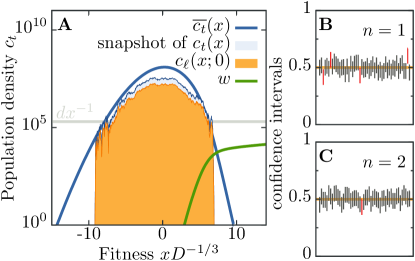
Figure 9: Fixation and extinction measurements with the trivial labelling of $c_{\ell}(x,0)=c(x,0)/2$. With such a labelling we obviously expect half of all simulations to end in fixation and half to end in extinction of the subpopulation $c_{\ell}$. The obtained confidence intervals serve as indicator for the noisiness of such measurements, when comparing results to the position depend labelling (cf. Eq. (70)) presented in Fig. 4. In general, however, the initial hypothesis of a fixation probability of $1/2$ is corroborated by simulation results (Panels BC).

From this configuration, we run the stochastic time evolution of the population until the labelled subpopulation either reaches fixation or goes extinct. In accordance with our interpretation of $u^{(n)}$ as fixation probability, we expect the labeled population to fix in half of the simulation runs and to go extinct otherwise. For definiteness, we abort simulations when one of the thresholds $\bigl{\langle}u^{(n)}\mid c_{\ell}\bigr{\rangle}=1-10^{-4}$ or $\bigl{\langle}u^{(n)}\mid c_{\ell}\bigr{\rangle}=10^{-4}$ is exceeded. We count such events as fixation and extinction, respectively.

After having amassed such simulation evidence, we can use Bayesian inference to check if our assumption of the interpretation of $u^{(n)}$ as fixation probability is consistent ohagan1994advanced . The distribution of the fixation probability $p_{\ell}^{\text{fix}}$ of the sub-population, given the (simulation-) data is computed as

$$\mathbb{P}\bigl{[}\,p_{\ell}^{\text{fix}}\,|\,\mathrm{data}\,\bigr{]}\sim\mathbb{P}\bigl{[}\,\mathrm{data}\,|\,p_{\ell}^{\text{fix}}\,\bigr{]}\,\mathbb{P}\bigl{[}\,p_{\ell}^{\text{fix}}\,\bigr{]}\;,$$ (71)

using Bayes’ theorem. Here, the likelihood $\mathbb{P}\bigl{[}\,\mathrm{data}\,|\,p_{\ell}^{\text{fix}}\,\bigr{]}$ of observing either an extinction or fixation event is a simple binomial distribution: when having $N$ trials with $X$ fixation events, the likelihood is $\mathbb{P}\bigl{[}\,X\,\mathrm{Fixation\,events}|\,p_{\ell}^{\text{fix}}\,\bigr{]}=\binom{N}{X}(p_{\ell}^{\text{fix}})^{X}(1-p_{\ell}^{\text{fix}})^{N-X}$. Furthermore, we assume a flat prior $\mathbb{P}\bigl{[}p_{\ell}^{\text{fix}}\bigr{]}$ for the fixation probability $p_{\ell}^{\text{fix}}$, ignoring any knowledge about its value at the beginning. Such a flat prior can also be cast as a Beta distribution (incidentally a conjugate prior ohagan1994advanced ), which in its general form is given by

$$\mbox{Beta}\bigl{(}Y;\alpha,\beta)\propto\frac{\Gamma(\alpha+\beta)}{\Gamma(\alpha)\Gamma(\beta)}Y^{\alpha-1}(1-Y)^{\beta-1}\;.$$ (72)

Using the two hyperparameters $\alpha=1$ and $\beta=1$ we arrive at the uniform (flat) distribution on $\bigl{[}0;1\bigr{]}$. Thus, the posterior distribution for the fixation probability $p_{\ell}^{\text{fix}}$ of the sub-population can also be written as Beta-distribution:

$$\mathbb{P}\bigl{[}\,p_{\ell}^{\text{fix}}\,|\,X\,\mathrm{Fixation\,events}\,\bigr{]}\sim(p_{\ell}^{\text{fix}})^{X+\alpha-1}(1-p_{\ell}^{\text{fix}})^{N-X+\beta-1}\;,~{}~{}\alpha=\beta=1\;,$$ (73)

up to a normalization factor. From this posterior (73) we can evaluate the $95\%$ confidence interval, and check if our assumption $p_{\ell}^{\text{fix}}=1/2$ is within its range. Increasing the value of $\alpha=\beta>1$ would increase the certainness of our initial hypothesis, $p_{\ell}^{\text{fix}}=1/2$, that we put into the model, narrowing the distribution (73).

References

- (1) L. J. Allen. An introduction to stochastic processes with applications to biology. Pearson Education New Jersey, 2003.
- (2) N. Barton, A. Etheridge, and A. Véber. Modelling evolution in a spatial continuum. Journal of Statistical Mechanics: Theory and Experiment, 2013(01):P01002, 2013.
- (3) E. Brunet and B. Derrida. Shift in the velocity of a front due to a cutoff. Physical Review E, 56(3):2597, 1997.
- (4) E. Brunet, B. Derrida, A. Mueller, and S. Munier. Phenomenological theory giving the full statistics of the position of fluctuating pulled fronts. Physical Review E, 73(5):056126, 2006.
- (5) E. Cohen, D. A. Kessler, and H. Levine. Fluctuation-regularized front propagation dynamics in reaction-diffusion systems. Physical review letters, 94(15):158302, 2005.
- (6) E. Cohen, D. A. Kessler, and H. Levine. Front propagation up a reaction rate gradient. Physical Review E, 72(6):066126, 2005.
- (7) M. M. Desai and D. S. Fisher. Beneficial mutation–selection balance and the effect of linkage on positive selection. Genetics, 176(3):1759–1798, 2007.
- (8) M. M. Desai, D. S. Fisher, and A. W. Murray. The speed of evolution and maintenance of variation in asexual populations. Current biology, 17(5):385–394, 2007.
- (9) M. M. Desai, A. M. Walczak, and D. S. Fisher. Genetic diversity and the structure of genealogies in rapidly adapting populations. Genetics, 193(2):565–585, 2013.
- (10) D. S. Fisher. Asexual evolution waves: fluctuations and universality. Journal of Statistical Mechanics: Theory and Experiment, 2013(01):P01011, 2013.
- (11) R. Frankham. Effective population size/adult population size ratios in wildlife: a review. Genetical research, 66(02):95–107, 1995.
- (12) P. J. Gerrish and R. E. Lenski. The fate of competing beneficial mutations in an asexual population. Genetica, 102:127–144, 1998.
- (13) L. Geyrhofer. Quantifying Evolutionary Dynamics. PhD thesis, MPI for Dynamics and Self-Organization, and University of Göttingen, 2014.
- (14) L. Geyrhofer and O. Hallatschek. Stochastic delocalization of finite populations. Journal of Statistical Mechanics: Theory and Experiment, 2013(01):P01007, 2013.
- (15) L. Geyrhofer and O. Hallatschek. Oscillations in noisy traveling waves. In preparation, 2015.
- (16) B. H. Good, I. M. Rouzine, D. J. Balick, O. Hallatschek, and M. M. Desai. Distribution of fixed beneficial mutations and the rate of adaptation in asexual populations. Proceedings of the National Academy of Sciences, 109(13):4950–4955, 2012.
- (17) I. Gordo, L. Perfeito, and A. Sousa. Fitness effects of mutations in bacteria. Journal of molecular microbiology and biotechnology, 21(1-2):20–35, 2011.
- (18) S. Goyal, D. J. Balick, E. R. Jerison, R. A. Neher, B. I. Shraiman, and M. M. Desai. Dynamic mutation–selection balance as an evolutionary attractor. Genetics, 191(4):1309–1319, 2012.
- (19) P. Haccou, P. Jagers, and V. A. Vatutin. Branching processes: variation, growth, and extinction of populations. Number 5. Cambridge University Press, 2005.
- (20) O. Hallatschek. The noisy edge of traveling waves. Proceedings of the National Academy of Sciences, 108(5):1783–1787, 2011.
- (21) O. Hallatschek and D. R. Nelson. Gene surfing in expanding populations. Theoretical population biology, 73(1):158–170, 2008.
- (22) D. Hedgecock and A. I. Pudovkin. Sweepstakes reproductive success in highly fecund marine fish and shellfish: a review and commentary. Bulletin of Marine Science, 87(4):971–1002, 2011.
- (23) G. S. Katzenberger. Solutions of a stochastic differential equation forced onto a manifold by a large drift. The Annals of Probability, pages 1587–1628, 1991.
- (24) E. Kussell and M. Vucelja. Non-equilibrium physics and evolution—adaptation, extinction, and ecology: a key issues review. Reports on Progress in Physics, 77(10):102602, 2014.
- (25) S. F. Levy, J. R. Blundell, S. Venkataram, D. A. Petrov, D. S. Fisher, and G. Sherlock. Quantitative evolutionary dynamics using high-resolution lineage tracking. Nature, 2015.
- (26) R. A. Neher. Genetic draft, selective interference, and population genetics of rapid adaptation. Annu. Rev. Ecol. Evol. Syst, 44:195–215, 2013.
- (27) R. A. Neher and O. Hallatschek. Genealogies of rapidly adapting populations. Proceedings of the National Academy of Sciences, 110(2):437–442, 2013.
- (28) R. A. Neher, T. A. Kessinger, and B. I. Shraiman. Coalescence and genetic diversity in sexual populations under selection. Proceedings of the National Academy of Sciences, 110(39):15836–15841, 2013.
- (29) R. A. Neher, B. I. Shraiman, and D. S. Fisher. Rate of adaptation in large sexual populations. Genetics, 184(2):467–481, 2010.
- (30) A. O’Hagan and J. Forster. Kendall’s Advanced Theory of Statistics: Bayesian Inference, volume 2B. New York Halsted Press, 1994.
- (31) F. Pelletier, D. Garant, and A. P. Hendry. Eco-evolutionary dynamics. Philosophical Transactions of the Royal Society B: Biological Sciences, 364(1523):1483–1489, 2009.
- (32) L. Perfeito, L. Fernandes, C. Mota, and I. Gordo. Adaptive mutations in bacteria: high rate and small effects. Science, 317(5839):813–815, 2007.
- (33) W. H. Press, S. A. Teukolsky, W. T. Vetterling, and B. P. Flannery. Numerical recipes 3rd edition: The art of scientific computing. Cambridge university press, 2007.
- (34) M. Reiter, S. Rulands, and E. Frey. Range expansion of heterogeneous populations. Physical review letters, 112(14):148103, 2014.
- (35) I. M. Rouzine, É. Brunet, and C. O. Wilke. The traveling-wave approach to asexual evolution: Muller’s ratchet and speed of adaptation. Theoretical population biology, 73(1):24–46, 2008.
- (36) I. M. Rouzine, J. Wakeley, and J. M. Coffin. The solitary wave of asexual evolution. Proceedings of the National Academy of Sciences, 100(2):587–592, 2003.
- (37) S. Schiffels, G. J. Szöllősi, V. Mustonen, and M. Lässig. Emergent neutrality in adaptive asexual evolution. Genetics, 189(4):1361–1375, 2011.
- (38) O. Tenaillon. The utility of fisher’s geometric model in evolutionary genetics. Annual Review of Ecology, Evolution, and Systematics, 45:179–201, 2014.
- (39) L. S. Tsimring, H. Levine, and D. A. Kessler. Rna virus evolution via a fitness-space model. Physical review letters, 76(23):4440, 1996.
- (40) N. G. Van Kampen. Stochastic processes in physics and chemistry, volume 1. Elsevier, 1992.
- (41) W. van Saarloos. Front propagation into unstable states. Physics reports, 386(2):29–222, 2003.
- (42) J. Wakeley. Coalescent theory: an introduction, volume 1. Roberts & Company Publishers Greenwood Village, Colorado, 2009.