Exit Probabilities and Balayage of Constrained Random Walks

Abstract

Let $X$ be the constrained random walk on ${\mathbb{Z}}_{+}^{d}$, $d\in\{2,3,4,...\}$, representing the queue lengths of a stable Jackson network and let $x\in{\mathbb{Z}}_{+}^{d}$ be its initial position ($X$ is a random walk with independent and identically distributed increments except that its dynamics are constrained on the boundaries of ${\mathbb{Z}}_{+}^{d}$ so that $X$ remains in ${\mathbb{Z}}_{+}^{d}$; stability means that $X$ has a nonzero drift pushing it to the origin). Let $\tau_{n}$ be the first time when the sum of the components of $X$ equals $n$. The probability $p_{n}\doteq P_{x}(\tau_{n}<\tau_{0})$ is one of the key performance measures for the queueing system represented by $X$ and its analysis/computation received considerable attention over the last several decades. The stability of $X$ implies that $p_{n}$ decays exponentially in $n$. Currently the only analytic method available to approximate $p_{n}$ is large deviations analysis, which gives the exponential decay rate of $p_{n}$. Finer approximations are available via rare event simulation. The present article develops a new method to approximate $p_{n}$ and related expectations. The method has two steps: 1) with an affine transformation, move the origin to a point on the exit boundary associated with $\tau_{n}$; let $n\rightarrow\infty$ to remove some of the constraints on the dynamics of the walk; the first step gives a limit unstable /transient constrained random walk $Y$ 2) construct a basis of harmonic functions of $Y$ and use this basis to apply the classical superposition principle of linear analysis (the basis functions can be seen as perturbations of the classical Fourier basis). The basis functions are linear combinations of $\log$-linear functions and come from solutions of harmonic systems; these are graphs with labeled edges whose vertices represent points on the interior characteristic surface ${\mathcal{H}}$ of $Y$; the edges between the vertices represent conjugacy relations between the points on the characteristic surface, the loops (edges from a vertex to itself) represent membership in the boundary characteristic surfaces. Characteristic surfaces are algebraic varieties determined by the distribution of the unconstrained increments of $X$ and the boundaries of ${\mathbb{Z}}_{+}^{d}$. Each point on ${\mathcal{H}}$ defines a harmonic function of the unconsrained version of $Y$. Using our method we derive explicit, simple and almost exact formulas for $P_{x}(\tau_{n}<\tau_{0})$ for $X$ representing $d$-tandem queues, similar to the product form formulas for the stationary distribution of $X$. The same method allows us to approximate the Balayage operator mapping $f$ to $x\rightarrow{\mathbb{E}}_{x}\left[f(X_{\tau_{n}})1_{\{\tau_{n}<\tau_{0}\}}\right]$ for a range of stable constrained random walks representing the queue lengths of a queueing system with two nodes (i.e., $d=2$). We provide two convergence theorems; one using the coordinates of the limit process and one using the scaled coordinates of the original process. The latter is given for two tandem queues (i.e., when the set of possible increments of $X$ is $\{(0,1),(-1,1)(0,-1)\}$) and uses a sequence of subsolutions of a related Hamilton Jacobi Bellman equation on a manifold; the manifold consists of three copies of ${\mathbb{R}}_{+}^{2}$, the zeroth glued to the first along $\{x:x(1)=0\}$ and the first to the second along $\{x:x(2)=0\}.$ We indicate how the ideas of the paper relate to more general processes and exit boundaries.

1 Introduction

Constrained random walks arise naturally as models of queueing networks and this paper treats only walks associated with Jackson networks. But the approach of the paper applies more generally, see subsection 9.3.

Let $X$ denote the number of customers in the queues of a $d$-node Jackson network at arrival and service completion times ($X_{k}(i)$ is the number of customers waiting in queue $i$ of the network right after the $k^{th}$ arrival/service completion); mathematically, $X$ is a constrained random walk on ${\mathbb{Z}}^{d}_{+}$, i.e., it has independent increments except that on the boundaries of ${\mathbb{Z}}^{d}_{+}$ the process is constrained to remain on ${\mathbb{Z}}^{d}_{+}$ (see (2) for the precise definition of the constrained random walk $X$). Define

$$A_{n}=\left\{x\in{\mathbb{Z}}_{+}^{d}:\sum_{i=1}^{d}x(i)\leq n\right\}$$ (1)

and its boundary

$$\partial A_{n}=\left\{x\in{\mathbb{Z}}_{+}^{d}:\sum_{i=1}^{d}x(i)=n\right\}.$$ (2)

Let $\tau_{n}$ be the first time $X$ hits $\partial A_{n}$. One of the “exit probabilities” that the title refers to is $p_{n}\doteq P_{x}(\tau_{n}<\tau_{0})$, the probability that starting from an initial state $x\in A_{n}$ the number of customers in the system reaches $n$ before the system empties. One of our primary aims in this paper will be the approximation of this probability. The set $A_{n}$ models a systemwide shared buffer of size $n$ (for example, if the queueing system models a set of computer programs running on a computer, the shared buffer may be the computer’s memory) and $\tau_{n}$ represents the first time this buffer overflows. If we measure time in the number of independent cycles that restart each time $X$ hits $0$, $p_{n}$ is the probability that the current cycle finishes successfully (i.e., without a buffer overflow).

One can change the domain $A_{n}$ to model other buffer structures, e.g., $\{x\in{\mathbb{Z}}_{+}^{d}:x(i)\leq n\}$ models separate buffers of size $n$ for each queue in the system. The present work focuses on the domain $A_{n}$. The basic ideas of the paper apply to other domains, and we comment on this in the conclusion.

For a set $a$ and $\tau_{a}\doteq\{k:X_{k}\in a\}$, the distribution ${\mathcal{T}}_{a}$ of $X_{\tau_{a}}$ on $a$ is called the Balayage operator. ${\mathcal{T}}_{a}$ maps bounded measurable functions on $a$ to harmonic functions on $a^{c}$:

$${\mathcal{T}}_{a}:f\rightarrow g,g(x)={\mathbb{E}}_{x}\left[f\left(X_{\tau_{a}}\right)1_{\{\tau_{a}<\infty\}}\right].$$

The computation of $p_{n}$ is a special case of the computation of (the image of a given function under) the Balayage operator: for $a=A_{n}^{c}\cup\partial A_{n}\cup\{0\}$, $\tau_{a}$ becomes $\tau_{n}\wedge\tau_{0}$ and if we set

$$f=1_{\{\partial A_{n}\}},$$

$({\mathcal{T}}_{a}f)(x)={\mathbb{E}}_{x}\left[f(X_{\tau_{a}})1_{\{\tau_{a}<\infty\}}\right]$, $x\in A_{n}$, equals $P_{x}(\tau_{n}<\tau_{0})$.

We assume that $X$ is stable, i.e., the total arrival rate $\nu_{i}$ is less than the total service rate $\mu_{i}$ for all nodes $i$ of the queueing system that $X$ represents ($\mu$ and $\nu$ are linear functions of the distribution of the increments of $X$, see (12) and (13) for their definitions). For a stable $X$, the event $\{\tau_{n}<\tau_{0}\}$ rarely happens and its probability $p_{n}$ decays exponentially with buffer size $n$. The problem of approximating $p_{n}$ has a long history and an extensive literature; let us mention two of the main approaches here. The first is large deviations (LD) analysis [4, 3, 15] which gives the exponential decay rate of $p_{n}$ as the value function of a limit deterministic optimal control problem (see below). If one would like to obtain more precise estimates than what LD analysis gives, the popular method has so far been simulation with variance reduction such as importance sampling, see, [1, Chapter VI] and [8, 5]; the use of IS for similar problems in a single dimension goes back to [16]. The goal of this paper is to offer a new alternative, which, in particular, allows to approximate the Balayage operator for a wide class of two dimensional systems and gives an almost exact formula for the probability $P_{x}(\tau_{n}<\tau_{0})$ for tandem networks in any dimension. We explain its elements in the following paragraphs.

One way to think of the LD analysis is as follows. $p_{n}$ itself decays to $0$, which is trivial. To get a nontrivial limit transform $p_{n}$ to $V_{n}\doteq-\frac{1}{n}\log p_{n}$; using convex duality, one can write the $-\log$ of an expectation as an optimization problem involving the relative entropy [4] and thus $V_{n}$ can be interpreted as the value function of a discrete time stochastic optimal control problem. The LD analysis consists of the law of large numbers limit analysis of this control problem; the limit problem is a deterministic optimal control problem whose value function satisfies a first order Hamilton Jacobi Bellman equation (see (148) of Section 7). Thus, LD analysis amounts to the computation of the limit of a convex transformation of the problem.

We will use another, an affine, transformation of $X$ for the limit analysis. The proposed transformation is extremely simple: observe $X$ from the exit boundary. The most natural vantage points on the exit boundary $\partial A_{n}$ are the corners $\{ne_{i},i=1,2,3,...,d\}$, where $e_{i}$ are the standard basis elements of ${\mathbb{Z}}^{n}$:

$$Y^{n}\doteq T_{n}(X),~{}~{}~{}T_{n}:{\mathbb{R}}^{d}\rightarrow{\mathbb{R}}^{d},T_{n}(x)\doteq y,~{}~{}~{}y(j)=\begin{cases}n-x(j),&\text{ if }j=i,\\ x(j)&\text{ otherwise},\end{cases}$$ (3)

$j=1,2,\cdots,d.$ $T_{n}$ is affine and its inverse equals itself. $Y^{n}$, i.e., the process $X$ as observed from the corner $ne_{i}$, is a constrained process on the domain $\Omega_{Y}^{n}\doteq{\mathbb{Z}}_{+}^{d}\times(n-{\mathbb{Z}}_{+})\times{\mathbb{Z}}_{+}^{d}$; it is the same process as $X$, except that $Y^{n}$ represents the state of the $i^{th}$ queue not by the number of customers waiting in queue $i$ but by the number of spots in the buffer not occupied by the customers in queue $i$. $T_{n}$ maps the set $A_{n}$ to $B_{n}\subset\Omega_{Y}^{n}$, $B_{n}\doteq T_{n}(A_{n})$; the corner $ne_{i}$ to the origin of $\Omega_{Y}^{n}$; the exit boundary $\partial A_{n}$ to $\partial B_{n}\doteq\{y\in\Omega_{Y}^{n},y(i)=\sum_{j=1,j\neq i}^{d}y(j)\}$; finally the constraining boundary $\{z\in{\mathbb{Z}}_{+}^{d},z(i)=0\}$ to

$$\{y\in{\mathbb{Z}}_{+}^{i-1}\times{\mathbb{Z}}\times{\mathbb{Z}}_{+}^{d-i}:y(i)=n\}.$$

As $n\rightarrow\infty$ the last boundary vanishes and $Y^{n}$ converges to the limit process $Y$ on the domain $\Omega_{Y}\doteq{\mathbb{Z}}_{+}^{i-1}\times{\mathbb{Z}}\times{\mathbb{Z}}_{+}^{d-i}$ and the set $B_{n}$ to

$$B\doteq\left\{y\in\Omega_{Y},y(i)\geq\sum_{j=1,j\neq i}^{d}y(j)\right\}.$$ (4)

Figure 1 sketches these transformations for the case of $X$ representing lengths of two tandem queues and for $i=1$ (the random walk $X$ represents tandem queues if its set of possible jumps are $e_{1}$, $-e_{i}+e_{i+1}$ , $i=1,2,3,...,d-1$ and $-e_{d}$, if $X$ is of this form we will call it a “tandem walk;” for the exact definition, see (15)).

Figure 1:    The transformation $T_{n}$

The boundary of $B$ is

$$\partial B=\left\{y\in\Omega_{Y},y(i)=\sum_{j=1,j\neq i}^{d}y(j)\right\};$$ (5)

the limit stopping time

$$\tau\doteq\inf\{k:Y_{k}\in\partial B\}$$ (6)

is the first time $Y$ hits $\partial B$. The stability of $X$ and the vanishing of the boundary constraint on $i$ implies that $Y$ is unstable / transient, i.e., with probability $1$ it wanders off to $\infty$. Therefore, in our formulation, the limit process is an unstable constrained random walk in the same space and time scale as the original process but with less number of constraints.

Fix an initial point $y\in B$ in the new coordinates; our first convergence result is Proposition 3.1 which says

$$p_{n}=P_{x_{n}}(\tau_{n}<\tau_{0})\rightarrow P_{y}(\tau<\infty),$$ (7)

where $x_{n}=T_{n}(y)$. The proof uses the law of large numbers and LD lowerbounds to show that the difference between the two sides of (7) vanishes with $n$. With (7) we see that the limit problem in our formulation is to compute the hitting probability of the unstable $Y$ to the boundary $\partial B$.

The convergence statement (7) involves a fixed initial condition for the process $Y$. In classical LD analysis, one specifies the initial point in scaled coordinates as follows: $x_{n}=\lfloor nx\rfloor\in A_{n}$ for $x\in{\mathbb{R}}_{+}^{d}$. Then the initial condition for the $Y^{n}$ process will be $y_{n}=T_{n}(x_{n})$ (thus we fix not the $y$ coordinate but the scaled $x$ coordinate). When $x_{n}$ is defined in this way, (7) becomes a trivial statement because its both sides decay to $0$. For this reason, Section 7 studies the relative error

$$\frac{|P_{x_{n}}(\tau_{n}<\tau_{0})-P_{y_{n}}(\tau<\infty)|}{P_{x_{n}}(\tau_{n}<\tau_{0})};$$ (8)

Proposition 7.1 says that this error converges exponentially to $0$ for the case of two dimensional tandem walk (i.e., the process $X$ shown in Figure 1). The proof rests on showing that the probability of the intersection of the events $\{\tau_{n}<\tau_{0}\}$ and $\{\tau<\infty\}$ dominate the probabilities of both as $n\rightarrow\infty$. For this we calculate bounds in Proposition 7.3 on the LD decay rates of the probability of the differences between these events using a sequence of subsolutions of a Hamilton Jacobi Bellman equation on a manifold; the manifold consists of three copies of ${\mathbb{R}}_{+}^{2}$, zeroth copy glued to the first along $\partial_{1}$, and the first to the second along $\partial_{2}$, where $\partial_{i}=\{x\in{\mathbb{R}}_{+}^{2}:x(i)=0\}.$ Extension of this argument to more complex processes and domains remains for future work.

For a process $X$ in $d$ dimensions, each affine transformation $T_{n}^{i}$, $i=1,2,3,...,d$, gives a possible approximation of $P_{x}(\tau_{n}<\tau_{0})$. A key question is: which of these best approximates $P_{x}(\tau_{n}<\tau_{0})$ for a given $x$? Proposition 7.1 says that, for the two dimensional tandem walk, $i=1$ works well for all points $x=\lfloor nx\rfloor$ as long as $x(1)>0$. In general this will not be the case (i.e., depending on $x$, removing one constraint of the process may give better approximations than removing another); subsection 7.1 comments on this problem.

The convergence results (7) and (8) reduce the problem of calculation of $P_{x}(\tau_{n}<\tau_{0})$ to that of $P_{y}(\tau<\infty)$. This constitutes the first step of our analysis and we expect it to apply more generally; see subsection 9.3. Computation of $P_{y}(\tau<\infty)$ is a static linear problem and can be attacked with a range of ideas and methods.

Sections 4, 5 and 6 apply the principle of superposition of classical linear analysis to the computation of $P_{y}(\tau<\infty)$ and related expectations. The key for its application is to construct the right class of efficiently computable basis functions to be superposed. The construction of our basis functions goes as follows: the distribution of the increments of $Y$ is used to define the characteristic polynomial ${\mathbf{p}}:{\mathbb{C}}^{n}\rightarrow{\mathbb{C}}$. ${\mathbf{p}}$ can be represented both as a rational function and as a polynomial; to simplify our analysis we use the polynomial representation in two dimensions and the rational one in $d$ dimensions. In the rest of this paragraph we will only refer to the higher dimensional definitions; the definitions for the case of two dimensions are given in subsection 4.1. We call the $1$ level set of ${\mathbf{p}}$, the characteristic surface of $Y$ and denote it with ${\mathcal{H}}$, see (98). ${\mathcal{H}}$ is, more precisely, a $d-1$ dimensional complex affine algebraic variety of degree $d+1$. Each point on the characteristic surface ${\mathcal{H}}$ defines a $\log$-linear function (see (95)) that satisfies the interior harmonicity condition of $Y$ (i.e., defines a harmonic function of the completely unconstrained version of $Y$); similarly, each boundary of the state space of $Y$ has an associated characteristic polynomial and surface. ${\mathbf{p}}$ can be written as a second order polynomial in each of its arguments; this implies that most points on ${\mathcal{H}}$ come in conjugate pairs, there are $d-1$ different conjugacy relations, one for each constraining boundary of $Y$. The keystone of the approach developed in these sections is the following observation: $\log$-linear functions defined by two points on ${\mathcal{H}}$ satisfying a given type of conjugacy relation can be linearly combined to get nontrivial functions which satisfy the corresponding boundary harmonicity condition (as well as the interior one); see Proposition 5.1. Based on this observation we introduce the concept of a harmonic system (Definition 5.2) which is an edge-complete graph with labeled edges representing a system of variables and equations: the vertices represent the variables constrained to be on ${\mathcal{H}}$, the edges between distinct vertices represent the conjugacy relations between the variables that the edges connect (the label of the edge determines the type of the conjugacy relation) and its loops (an edge from a vertex to itself) represent membership on a boundary characteristic surface (the label of the loop determines which boundary characteristic surface). We show that any solution to a harmonic system gives a harmonic function for $Y$ in the form of linear combinations of $\log$-linear functions (each vertex defines a $\log$-linear function). The computational complexity of the evaluation of the resulting harmonic function is essentially determined by the size of the graph.

In two dimensions (Section 4) edge-complete graphs have $1$ or $2$ vertices and the above construction gives a rich enough basis of harmonic functions of $Y$ to approximate the image of any function on $\partial B$ under the Balayage operator; with the use of these basis functions the approximation of ${\mathbb{E}}_{y}[f(Y_{\tau})1_{\{\tau<\infty\}}]$ for any given bounded $f$ reduces to the solution of a linear equation in $K$ dimensions, where $K$ is the number of basis functions used in the approximation (Section 8.2 gives an example with $K=12$). Once the approximation is computed, the error made in the approximation is simple to bound when $f$ is constant outside of a bounded support and satisfies $f>0$ or $f<0$. The restrictions of the basis functions on ${\partial B}$ are perturbed versions of the restriction of the ordinary Fourier basis on ${\mathbb{Z}}$ to ${\mathbb{Z}}_{+}$; for this reason we call the constructed basis a “perturbed” Fourier basis.

Section 5 gives the definition of a harmonic system for $d$-dimensional constrained walks and prove that any solution to a harmonic system defines a $Y$-harmonic function (Proposition 5.2). In Section 6 we compute explicit solutions to a particular class of harmonic systems for the $d$ dimensional tandem walk; the span of the class contains $P_{y}(\tau<\infty)$ exactly. Hence we obtain explicit formulas, similar to the product form formulas for the stationary distribution of Jackson networks [10], for $P_{y}(\tau<\infty)$ in the case of constrained walks representing tandem queues in arbitrary dimension (see Proposition 6.5; the two dimensional version of the same formula is written out more explicitly in display (163)). If we take exponentiation and algebraic operations to be atomic, the complexity of evaluating the formula is independent of $y$ (and hence of the buffer size $n$ if $P_{y}(\tau<\infty)$ is used to approximate $P_{x}(\tau_{n}<\tau_{0})$ ) and depends only on the dimension $d$ of $X$.

Section 8 gives example computations using the approach developed in the paper. Three examples are considered: the tandem walk in two dimensions, a non tandem walk in two dimensions, tandem walk in $4$ and $14$ dimensions. The conclusion (Section 9) discusses several directions for future research. Among these are the application of the approach of the present paper to constrained diffusion processes (subsection 9.1), the study of nonlinear perturbed second order HJB equations which arise when one would like to sharpen large deviations estimates (subsection 9.2) and the sizes of boundary layers which arise in subsolution based IS algorithms applied to constrained random walks (subsection 9.5).

2 Definitions

This section sets the notation of the paper, defines the domains, the processes and the stopping times we will study and states some elementary facts about them.

We will denote components of a vector using parentheses, e.g., for $x\in{\mathbb{Z}}_{+}^{d}$, $x(i)$, $i=1,2,3,...,d$ denotes the $i^{th}$ component of $x$.

For two sets $a$ and $b$, $a^{b}$ denotes the set of functions from $b$ to $a$. For a function $f$ on a set $a$, we will write $f|_{c}$ to mean $f$’s restriction to a subset $c\subset a$. For a finite set $a$, $|a|$ denotes the number of its elements. We will assume that elements of sets are written in a certain order and we will index sets as we index vectors, e.g., $a(1)$ denotes the first element of $a$ and $a(|a|)$ the last.

Our analysis will involve several types of boundaries: the coordinate hyperplanes of ${\mathbb{Z}}^{d}$, the constraining boundaries of constrained processes and the boundaries of exit sets. To keep our notation short and manageable, we will make use of the symbol $\partial$ to indicate that a set is a boundary of some type.

Define ${\mathcal{N}}_{0}\doteq\{0,1,2,...,d\}$ and ${\mathcal{N}}_{+}\doteq{\mathcal{N}}_{0}-\{0\}$; ${\mathcal{N}}_{+}$ is the set of nodes of $X$. For $a\subset{\mathcal{N}}_{+}$ the coordinate hyperplanes of ${\mathbb{Z}}^{d}$ are

$$\partial_{a}\doteq\left\{z\in{\mathbb{Z}}^{d},~{}z(j)=0~{}\forall j\in a\right\}.$$

We will use the letter $\sigma$ to denote hitting times to these sets; for any process ${\mathcal{P}}$ on ${\mathbb{Z}}^{d}$ define

$$\sigma^{\mathcal{P}}_{a}\doteq\inf\{k:{\mathcal{P}}_{k}\in\partial_{a}\};$$ (9)

in what follows the process ${\mathcal{P}}$ will always be clear from context and we will omit the superscript of $\sigma$. If $a=\{j\}$ for some $j\in{\mathcal{N}}_{+}$, we will write $\sigma_{j}$ rather than $\sigma_{\{j\}}$; the same convention applies to $\partial_{\{j\}}.$

We will denote the domain of a process ${\mathcal{P}}$ by $\Omega_{\mathcal{P}}$; $\partial\Omega_{\mathcal{P}}$ will denote its constraining boundary if it has one; $\Omega_{\mathcal{P}}^{o}$ will denote $\Omega_{\mathcal{P}}-\partial\Omega_{\mathcal{P}}$.

We will often express constraints of constrained random walks using the constraining maps $\pi_{a}$, $a\subset{\mathcal{N}}_{+}$, defined as follows:

$$\pi_{a}(x,v)=\begin{cases}x+v,&\text{ if $x(j)+v(j)\geq 0~{}~{}\forall j\in a^{c}$},\\ x,&\text{ otherwise,}\end{cases}$$

where $x\in{\mathbb{Z}}^{d}$ and $v\in{\mathbb{Z}}^{d}$. If $a=\emptyset$, we will write $\pi$ instead of $\pi_{\emptyset}$; $\pi$ constrains to ${\mathbb{Z}}_{+}^{d}$ any process to which it is applied (see the definition of $X$ and $Y$ below to see how $\pi_{a}$ is used to define constrained random walks). Other than $a=\emptyset$ this paper will only use $\pi_{\{i\}}$, $i\in{\mathcal{N}}_{+}$ and for most of the paper we will assume $i=1$. To ease notation we will write $\pi_{i}$ rather than $\pi_{\{i\}}$; $\pi_{i}$ constrains a given process to be positive in its ${\mathcal{N}}_{+}-\{i\}$ coordinates.

If ${\mathcal{P}}$ is a random walk with increments ${\mathcal{V}}({\mathcal{P}})$, constrained to stay in $\Omega_{\mathcal{P}}\subset{\mathbb{Z}}^{d}$, and $S\subset\Omega_{\mathcal{P}}$, define

$$S^{o}\doteq\{s\in S:\Omega_{\mathcal{P}}\cap(s+{\mathcal{V}}({\mathcal{P}}))\subset S\},\partial S\doteq S-S^{o}.$$ (10)

The notation doesn’t state explicitly the ${\mathcal{P}}$-dependence of these terms; but whenever we use them below, the underlying process ${\mathcal{P}}$ will always be clear from context. In what follows ${\mathcal{P}}$ will be either $X$, $Y^{n}$, $Y$ or $Z$, all of which are defined below.

We want to compute certain probabilities/ expectations associated with a constrained random walk. This will involve three transformations of the original process: an affine change of variables, taking a limit (this will drop one of the boundary constraints of the process) and removing all constraints which makes the process an ordinary random walk with independent and identically distributed (iid) increments. We will show the original process with $X$, the result of the affine transformation with $Y^{n}$, the limit process with $Y$ and the completely unconstrained process with $Z$.

$X$ will denote a constrained random walk on $\Omega_{X}\doteq{\mathbb{Z}}_{+}^{d}$ with independent increments $I_{k}\in\{e_{i}-e_{j},i\neq j\in{\mathcal{N}}_{0}\}$ where $e_{0}$ is the zero vector in ${\mathbb{Z}}^{d}$ and $e_{i}\in{\mathbb{Z}}^{d}$, $i\neq 0$ is the unit vector in the direction $i$. To keep $X$ in its domain, the increments are constrained on the boundaries of ${\mathbb{Z}}_{+}^{d}$:

$$X_{0} =x\in{\mathbb{Z}}_{+}^{d},$$

$$X_{k+1} \doteq X_{k}+\pi(X_{k},I_{k})$$ (11)

$$\pi(x,e_{i}-e_{j}) \doteq\begin{cases}e_{i}-e_{j},&\text{ if }x(j)>0\\ 0,&\text{otherwise.}\end{cases},$$

where, by convention, “$x(0)$” means “$1$” (or some other positive quantity). The constraining boundary of $X$ is $\partial\Omega_{X}\doteq\Omega_{X}\cap\left(\cup_{j\in{\mathcal{N}}_{+}}\partial_{j}\right).$

We denote the common distribution of the increments $I_{k}$ by the matrix $p$, i.e., $p(i,j)$ is the probability that $I_{k}$ equals $e_{i}-e_{j}$, $i\neq j\in{\mathcal{N}}_{0}$; $p(i,i)=0$ for $i\in{\mathcal{N}}_{0}$. ${\mathcal{V}}(X)$ will denote the set of increments of $I_{k}$ with nonzero probability:

$${\mathcal{V}}(X)\doteq\{e_{i}-e_{j}:p(i,j)>0\}.$$

Remark 1.

For $v=e_{i}-e_{j}$, $i,j\in{\mathcal{N}}_{0}\times{\mathcal{N}}_{0}$, “$p(v)$” will denote $p(i,j)$.

For our probability space we will take ${\mathcal{V}}(X)^{\mathbb{N}}$. $\{I_{k}\}$ are the coordinate maps on ${\mathcal{V}}(X)^{\mathbb{N}}$, ${\mathscr{F}}$ is the $\sigma$-algebra generated by $\{I_{k}\}$ and $P$ is the product measure on ${\mathcal{V}}(X)^{\mathbb{N}}$ under which $I_{k}$ are an iid sequence with common distribution $p$.

$X$ describes the dynamics of the number of customers in the queues of a Jackson network, i.e., a queueing system with exponentially and identically distributed and independent interarrival and service times. In this interpretation, $0\in{\mathcal{N}}_{0}$ represents the outside of the queueing system and for $i\in{\mathcal{N}}_{+}$, $X_{k}(i)$ is the number of customers in queue $i$ at the $k^{th}$ jump of the system (an arrival or a service completion). $X$ is on the boundary $\partial_{i}$ when the $i^{th}$ queue is empty and the constrained dynamics on the boundary means that the server at node $i$ cannot serve when its queue is empty. The increment $e_{i}-e_{j}$, $i,j\neq 0$, $i\neq j$, represents a customer leaving queue $i$ after service completion at node $i$ and joining queue $j$; $e_{i}$, $i\neq 0$, represents an arrival from outside to queue $i$ and $-e_{j}$ a customer leaving the system after a server completion at queue $j$. We will assume that the Markov chain defined by the matrix $p$ on ${\mathcal{N}}_{0}$ is irreducible. One can also represent $p$ as arrival, service and routing probabilities:

$$\lambda_{j}\doteq p(0,j),~{}~{}\mu_{j}\doteq\sum_{j\in{\mathcal{N}}_{0}}p(j,k),j\in{\mathcal{N}}_{+},~{}~{}r(i,j)\doteq p(i,j)/\mu_{i}.$$ (12)

The irreducibility of $p$ implies that

$$\nu=\lambda+r\nu$$ (13)

has a unique solution. $\nu_{i}$ is the total arrival rate to node $i$ when system is in equilibrium. We assume that the network corresponding to $X$ is stable, i.e,

$$\rho_{i}\doteq\frac{\nu_{i}}{\mu_{i}}<1,~{}~{}i\in{\mathcal{N}}_{+}.$$ (14)

We will pay particular attention to tandem networks, i.e., a number of queues in tandem; these are Jackson networks whose $p$ matrix is of the form

$$p(0,1)>0,p(0,j)=0,j\neq 1,p(d,0)=\mu_{d},p(j,j+1)=\mu_{j},j\in{\mathcal{N}}_{0}-\{0,d\};$$ (15)

for tandem queues $\lambda$ will denote the only nonzero arrival rate $p(0,1)$; then $\nu_{i}=p(0,1)=\lambda$ for all $i\in{\mathcal{N}}_{+}$. We will call the random walk $X$ a tandem walk if it represents the queue lengths of a tandem network.

The domain $A_{n}$ is defined as in (1). We will assume

$$\lambda_{j}>0\text{ at least for some }j\in{\mathcal{N}}_{+}.$$ (16)

With this and (10), $\partial A_{n}$ indeed equals the right side of (2). Define the stopping times

$$\tau_{n}\doteq\{k:X_{k}\in\partial A_{n}\}$$

and

$$p_{n}\doteq P(\tau_{n}<\tau_{0}).$$

If (16) fails, $p_{n}$ becomes trivial.

Define the input/output ratio of the system as

$$r\doteq\frac{\sum_{j\in{\mathcal{N}}_{+}}p(0,j)}{\sum_{j\in{\mathcal{N}}_{+}}p(j,0)}.$$ (17)

Stability of $X$ implies

Proposition 2.1.

$$r<1.$$ (18)

Proof.

By definition

$$p(0,j)=\nu_{j}-\sum_{k\in\{j\}^{c}}r(k,j)\nu_{k},$$

for $j\in{\mathcal{N}}_{+}$. Sum both sides over $j$:

$$\sum_{j\in{\mathcal{N}}_{+}}p(0,j) =\sum_{j\in{\mathcal{N}}_{+}}\nu_{j}(1-\sum_{k\in\{j\}^{c}}r(j,k))$$

$$=\sum_{j\in{\mathcal{N}}_{+}}\nu_{j}\frac{p(j,0)}{\mu_{j}}=\sum_{j\in{\mathcal{N}}_{+}}\rho_{j}p(j,0).$$

Then

$$r=\frac{\sum_{j\in{\mathcal{N}}_{+}}p(0,j)}{\sum_{j\in{\mathcal{N}}_{+}}p(j,0)}=\sum_{j\in{\mathcal{N}}_{+}}\rho_{j}\frac{p(j,0)}{\sum_{j\in{\mathcal{N}}_{+}}p(j,0)}$$

which is an average of the utilization rates $\rho_{i}$ which are by assumption all less than $1$; (18) follows. ∎

$T_{n}$ and $Y^{n}$ are defined as in (3). $T_{n}$ depends on $i$; when we need to make this dependence explicit we will write $T^{i}_{n}$; for most of the analysis of the paper $i$ will be fixed and therefore can be assumed constant, and, unless otherwise noted, in the following sections we will take $i=1$.

Define

$${\mathcal{I}}_{i}\in{\mathbb{R}}^{d\times d},~{}~{}{\mathcal{I}}_{i}(j,k)=0,j\neq k,~{}~{}{\mathcal{I}}_{i}(j,j)=1,i\neq j,~{}~{}{\mathcal{I}}_{i}(i,i)=-1.$$ (19)

${\mathcal{I}}_{i}$ is the identity operator except that its $i^{th}$ diagonal term is $-1$ rather than $1$. Then

$$T_{n}=ne_{i}+{\mathcal{I}}_{i}.$$ (20)

Define the sequence of transformed increments

$$J_{k}\doteq{\mathcal{I}}_{i}(I_{k});$$ (21)

$J_{k}$ and $I_{k}$ take the same values except that $J_{k}=e_{j}+e_{i}$ whenever $I_{k}=e_{j}-e_{i}$ and $J_{k}=-e_{i}$ whenever $I_{k}=e_{i}$. Define

$${\mathcal{V}}(Y)\doteq\{{\mathcal{I}}_{i}v,v\in{\mathcal{V}}(X)\}.$$

Remark 2.

For $v\in{\mathcal{V}}(Y)$ we will shorten $p({\mathcal{I}}_{i}v)$ to $p(v)$ (remember, per Remark 1, for $e_{i}-e_{j}$, $i,j\in{\mathcal{N}}_{0}$, $p(v)$ denotes $p(i,j)$).

The limit unstable constrained process $Y$ is

$$Y_{0}\doteq y\in{\mathbb{Z}}_{+}^{d},~{}~{}Y_{k+1}\doteq Y_{k}+\pi_{i}(Y_{k},J_{k}).$$ (22)

$Y$ has the same dynamics as $Y^{n}$ except that $Y$ has no constraining boundary on its $i^{th}$ coordinate; therefore its state space is $\Omega_{Y}\doteq{\mathbb{Z}}_{+}^{i-1}\times{\mathbb{Z}}\times{\mathbb{Z}}_{+}^{d-i}.$ The domain $B$ for $Y$ is defined as in (4) and its boundary $\partial B$ is defined from $B$ using (10) and coincides with the right side of (5). Let $\tau$ be as in (6). Define

$$\zeta_{n}\doteq\inf\left\{k:Y_{k}(i)=\sum_{j\neq i}Y_{k}(j)+n\right\};$$ (23)

note $\tau=\zeta_{0}.$

$X$, $Y^{n}$ and $Y$ are all defined on the same probability space $\left({\mathcal{V}}(X)^{\mathbb{N}},{\mathscr{F}},P\right)$; the measure $P$ and their initial positions determine their distributions. We will use a subscript on $P$ to denote the initial positions, e.g., $P_{x}(\tau_{n}<\tau_{0})$ is the same as $P(\tau_{n}<\tau_{0})$ with $X_{0}=x$ and $P_{y}(\tau<\infty)$ means $P(\tau<\infty)$ with $Y_{0}=y$.

We note a basic fact about $Y$ here:

Proposition 2.2.

For $y\in{\mathbb{Z}}_{+}^{d}$, $\sum_{i=1}^{d}y(i)<n$

$$P_{y}(\zeta_{n}\wedge\zeta_{0}=\infty)=0.$$ (24)

Proof.

Set

$$c=\sum_{j\in{\mathcal{N}}_{0}}p(0,j)>0.$$

For $y\in{\mathbb{Z}}_{+}^{d}$, $y:\sum_{i=1}^{d}y(i)<n$,

$$P_{y}(\zeta_{n}\wedge\zeta_{0}\leq n)>c^{\prime}\doteq c^{n}>0$$ (25)

because, at least the sample paths whose increments consist only of $\{-e_{i},i\in{\mathcal{N}}_{+},p(0,i)>0\}$ push $Y$ to $\partial B$ in $n$ steps and the probability of this event is $c^{n}$.

$\hat{Y}_{k}\doteq Y_{nk\wedge\zeta_{n}\wedge\zeta_{0}}$ is Markov on $\hat{B}_{n}\doteq\left\{y\in{\mathbb{Z}}_{+}^{d},0\leq\sum_{i=1}^{d}y(i)\leq n\right\}$ (because $Y$ is Markov). The boundary of the last set is

$$\partial\hat{B}_{n}=\left\{y\in{\mathbb{Z}}_{+}^{d},0=\sum_{i=1}^{d}y(i)\text{ or }\sum_{i=1}^{d}y(i)=n\right\}.$$

By definition

$$P_{y}(\zeta_{0}\wedge\zeta_{n}=\infty)\leq P_{y}(\hat{Y}_{k}\in\hat{B}_{n}-\partial\hat{B}_{n}).$$ (26)

The bound (25) implies $P_{y}\left(\hat{Y}_{1}\in\hat{B}_{n}-\partial\hat{B}_{n}\right)\leq 1-c^{\prime}.$ This and that $\hat{Y}$ is Markov give
$P_{y}\left(\hat{Y}_{k}\in\hat{B}_{n}-\partial\hat{B}_{n}\right)\leq(1-c^{\prime})^{k}.$ This and (26) imply

$$P_{y}(\zeta_{0}\wedge\zeta_{n}=\infty)\leq(1-c^{\prime})^{k}.$$ (27)

Letting $k\rightarrow\infty$ gives (24). ∎

3 Convergence - initial condition set for $Y$

This section shows that the affine transformation of observing the process from the exit boundary really gives approximations of the exit probabilities we seek to compute. The present convergence result specifies the initial point for the $Y$ process. This allows a simple argument that works for general stable $X$ and uses LD results only roughly to prove that certain probabilities decay to $0$. In Section 7 we will prove a second convergence result (for the case of two dimensional tandem walk) where the initial point is given for the $X$ process; this will require a finer use of large deviations decay rates.

Denote by ${\mathcal{X}}$ the law of large numbers limit of $X$ , i.e., the deterministic function which satisfies

$$\lim_{n}P_{x_{n}}\left(\sup_{k\leq t_{0}n}|X_{k}/n-{\mathcal{X}}_{k/n}|>\delta\right)=0$$ (28)

for any $\delta>0$ and $t_{0}>0$ where $x_{n}\in{\mathbb{Z}}_{+}^{d}$ is a sequence of initial positions satisfying $\frac{x_{n}}{n}\rightarrow\chi\in{\mathbb{R}}_{+}^{d}$ (see, e.g., [13, Proposition 9.5] or [2, Theorem 7.23]). The limit process starts from ${\mathcal{X}}_{0}=\chi$, is piecewise affine and takes values in ${\mathbb{R}}_{+}^{d}$; then $s_{t}\doteq\sum_{i=1}^{d}{\mathcal{X}}_{t}(i)$ starts from $\sum_{i}\chi(i)$ is also piecewise linear and continuous (and therefore differentiable except for a finite number of points) with values in ${\mathbb{R}}_{+}$. The stability and bounded iid increments of $X$ imply that $s$ is strictly decreasing and

$$c_{1}>-\dot{s}>c_{0}>0$$ (29)

for two constants $c_{1}$ and $c_{0}$. These imply that ${\mathcal{X}}$ goes in finite time $t_{1}$ to $0\in{\mathbb{R}}_{+}^{d}$ and remains there afterward.

Fix an initial point $y\in\Omega_{Y}$ for the process $Y$ and set $x_{n}=T_{n}(y)$; (20) implies

$$\frac{x_{n}}{n}\rightarrow e_{i}.$$ (30)

Proposition 3.1.

Let $y$ and $x_{n}$ be as above. Then

$$\lim_{n\rightarrow\infty}P_{x_{n}}(\tau_{n}<\tau_{0})=P_{y}(\tau<\infty).$$

Proof.

Note that for $n>y(i)$, $x_{n}\in A_{n}$. Define

$$M_{k}=\max_{l\leq k}Y_{l}(i),~{}~{}M^{X}_{k}=\min_{l\leq k}X_{l}(i).$$

$M$ is an increasing process and $M_{\tau}$ is the greatest that the $i^{th}$ component of $Y$ gets before hitting $\partial B$ (if this happens in finite time). The monotone convergence theorem implies

$$P_{y}(\tau<\infty)=\lim_{n\nearrow\infty}P_{y}(\tau<\infty,M_{\tau}<n).$$

Thus

$$P_{y}(\tau<\infty)=P_{y}(\tau<\infty,M_{\tau}<n)+P_{y}(\tau<\infty,M_{\tau}\geq n)$$ (31)

and the second term goes to $0$ with $n$. Decompose $P_{x_{n}}(\tau_{n}<\tau_{0})$ similarly using $M^{X}$:

$$P_{x_{n}}(\tau_{n}<\tau_{0}) =P_{x_{n}}\left(\tau_{n}<\tau_{0},M^{X}_{\tau_{n}}>0\right)+P_{x_{n}}\left(\tau_{n}<\tau_{0},M^{X}_{\tau_{n}}=0\right).$$

On the set $$\{M^{X}_{\tau_{n}}>0\} X \partial_{i} \tau_{n} \{\tau_{n}<\tau_{0}\} \{\tau<\infty\} X Y (T_{n}(X),n-M^{X}) (Y,M) \tau_{n}.$$, the process cannot reach the boundary before , therefore over this set 1) the events and coincide (remember that and are defined on the same probability space) 2) the distribution of is the same as that of upto time Therefore,

$$=P_{y}(\tau<\infty,M_{\tau}<n)+P_{x_{n}}\left(\tau_{n}<\tau_{0},M^{X}_{\tau_{n}}=0\right).$$

The first term on the right equals the first term on the right side of (31). We know that the second term in (31) goes to $0$ with $n$. Then to finish our proof, it suffices to show

$$\lim_{n}P_{x_{n}}\left(\tau_{n}<\tau_{0},M^{X}_{\tau_{n}}=0\right)=0.$$ (32)

$M^{X}_{\tau_{n}}=0$ means that $X$ has hit $\partial_{i}$ before $\tau_{n}$. Then the last probability equals

$$P_{x_{n}}\left(\sigma_{i}<\tau_{n}<\tau_{0}\right),$$ (33)

which, we will now argue, goes to $0$ ($\sigma_{i}$ is the first time $X$ hits $\partial_{i}$; see (9)). (30) implies ${\mathcal{X}}_{0}=e_{i}.$ Define $t^{i}\doteq\inf\{t:{\mathcal{X}}_{t}(i)=0\}$ and $t^{0}\doteq\inf\{t:{\mathcal{X}}_{t}=0\in{\mathbb{R}}^{d}\}.$ By definition $t^{i}\leq t^{0}<\infty$ Now choose $t_{0}$ in (28) to be equal to $t^{0}$, define ${\mathcal{C}}_{n}\doteq\left\{\sup_{k\leq t^{0}n}\in|X_{k}/n-{\mathcal{X}}_{k/n}|>\delta\right\}$ and partition (33) with ${\mathcal{C}}_{n}$:

$$P_{x_{n}}\left(\sigma_{i}<\tau_{n}<\tau_{0}\right)=P_{x_{n}}\left(\{\sigma_{i}<\tau_{n}<\tau_{0}\}\cap{\mathcal{C}}_{n}\right)+P_{x_{n}}\left(\{\sigma_{i}<\tau_{n}<\tau_{0}\}\cap{\mathcal{C}}_{n}^{c}\right).$$ (34)

The first of these goes to $0$ by (28). The event in the second term is the following: $X$ remains at most $n\delta$ distance away $n{\mathcal{X}}$ until its $nt^{0}$ step, hits $\partial_{i}$ then $\partial A_{n}$ and then $0$. These and (29) imply that, for $n$ large enough, any sample path lying in this event can hit $\partial A_{n}$ only after time $nt^{0}$. Thus, the second probability on the right side of (34) is bounded above by

$$P_{x_{n}}(\{nt^{0}<\tau_{n}<\tau_{0}\}\cap{\mathcal{C}}_{n}^{c}).$$

The Markov property of $X$, $\{\sigma_{i}<\tau_{n}<\tau_{0}\}\subset\{\tau_{n}<\tau_{0}\}$ and (28) imply that the last probability is less than

$$\sum_{x:|x|\leq n\delta}P_{x}(\tau_{n}<\tau_{0})P_{x_{n}}(X_{nt^{0}}=x).$$

For $|x|\leq n\delta$, the probability $P_{x}(\tau_{n}<\tau_{0})$ decays exponentially in $n$ [8, Theorem 2.3]; then, the above sum goes to $0$. This establishes (32) and finishes the proof of the proposition.

∎

4 Analysis of $Y$, $d=2$

Let us begin with several definitions for the general dimension $d$; because we will almost exclusively work with the $Y$ process from here on, we will shorten ${\mathcal{V}}(Y)$ to ${\mathcal{V}}$. A function $V:{\mathbb{Z}}^{d}\rightarrow{\mathbb{C}}$ is said to be a harmonic function of the process $Y$ (or $Y$-harmonic) on a set $O\subset\Omega_{Y}$ if

$$V(y)={\mathbb{E}}_{y}\left[V(Y_{1})\right]=\sum_{v\in{\mathcal{V}}}V(y+\pi_{i}(y,v))p(v),y\in O,$$ (35)

where we use the convention set in Remark 2. Throughout the paper $O$ will be either $B^{o}$ or $\Omega_{Y}$, and the choice will always be clear from context; for this reason we will often write “…is $Y$-harmonic” without specifying the set $O$. $V$ is said to be $Z$-harmonic on $O\subset{\mathbb{Z}}^{d}$ if

$$V(z)={\mathbb{E}}_{z}\left[V(Z_{1})\right]=\sum_{v\in{\mathcal{V}}}V(z+v))p(v),z\in O.$$

$Z$-harmonicity and $Y$-harmonicity coincide on $\Omega_{Y}^{o}$.

Above we have assumed the domain of $V$ to be ${\mathbb{Z}}^{d}.$ If $V$ is defined only on a subset $a\subset{\mathbb{Z}}^{d}$, it can be trivially extended to all ${\mathbb{Z}}^{d}$ by setting it to $0$ on ${\mathbb{Z}}^{d}-a$. Thus, the above definitions can be applied to any function defined on any subset of ${\mathbb{Z}}^{d}$; we will use a similar convention for most of the definitions below.

The Markov property of $Y$ implies that

$$h:y\rightarrow{\mathbb{E}}_{y}\left[f\left(Y_{\tau}\right)1_{\{\tau<\infty\}}\right],y\in B,$$ (36)

is a harmonic function of $Y$ whenever the right side is well defined for all $y\in B^{o}$. Note that $h$ is the image of the function $f$ under the Balayage operator ${\mathcal{T}}_{(B^{o})^{c}}$. The dynamics of $Y$ and the definition of $B$ imply that ${\mathcal{T}}_{(B^{o})^{c}}$ is a distribution on $\partial B$; for this reason we will call harmonic functions of the form (36) $\partial B$-determined. If a function $f$ is defined over a domain larger than $B$, we will call $f$ $\partial B$-determined, if its restriction to $B$ is so.

The analysis of the previous section suggests that we approximate

$$P_{x}(\tau_{n}<\tau_{0})$$

with $W(T_{n}(x))$ where

$$W(y)\doteq P_{y}(\tau<\infty)={\mathbb{E}}_{y}\left[1_{\{\tau<\infty\}}\right]$$ (37)

for any stable Jackson network $X$. $W$ is a $\partial B$ determined harmonic function of $Y$, in particular it solves (35) with $O=B^{o}$. That $W(y)=P_{y}(\tau<\infty)=1$ for $y\in\partial B$ implies that $W$ also satisfies the boundary condition

$$V|_{\partial B}=1.$$ (38)

Then $W$ is a solution of (35,38) with $O=B^{o}.$ Large deviations analysis of $W$ is an asymptotic analysis of the system (35,38) that scales $V$ to $-\frac{1}{n}\log V$ and uses a law of large numbers scaling for space and time. With the $y$ coordinates, we no longer need to scale $V$, time or space and can directly attempt to solve (35,38)- perhaps approximately. We have assumed that $X$ is stable; this implies that $Y_{\tau\wedge k}$, $k=1,2,3,...$, is unstable and therefore, the Martin boundary of this process has points at infinity. Then one cannot expect all harmonic functions of $Y$ to be $\partial B$-determined and in particular the system (35,38) will not have a unique solution; hence, once we find a solution of (35, 38) that we believe (approximately) equal to $P_{y}(\tau<\infty)$, we will have to prove that it is $\partial B$-determined.

Define

$$B_{Z}\doteq\left\{z\in{\mathbb{Z}}^{d}:z(1)\geq\sum_{j=2}^{d}z(j)\right\}.$$

The unconstrained version of (35) is

$$V(z)={\mathbb{E}}_{z}\left[V(Z_{1})\right]=\sum_{v\in{\mathcal{V}}}V(z+v)p(v),$$ (39)

$z\in O\subset{\mathbb{Z}}^{d}$ and that of (38) is

$$V|_{\partial B_{Z}}=1.$$ (40)

A function is said to be a harmonic function of the unconstrained random walk $Z$ on $O$ if it satisfies (39).

Introduce also the boundary condition

$$V|_{\partial B}=f,~{}~{}~{}f:\partial B\rightarrow{\mathbb{C}},$$ (41)

for $Y$ which generalizes (38).

Our idea to [approximately] solve (35,38) is this:

1. Construct a class ${\mathcal{F}}_{Y}$ of “simple” harmonic functions for the process $Y$ (i.e., a class of solutions to (35)) For this

   1. Construct a class ${\mathcal{F}}_{Z}$ of harmonic functions for the unconstrained process $Z$ (i.e., a class of solutions to (39) with $O={\mathbb{Z}}^{d}$),

   2. Use linear combinations of elements of ${\mathcal{F}}_{Z}$ to find solutions to (35).

2. Represent [or approximate] the boundary condition (38) by linear combinations of the boundary values of the $\partial B$-determined members of the class ${\mathcal{F}}_{Y}$.

The definition of the class ${\mathcal{F}}_{Z}$ is given in (51) and that of ${\mathcal{F}}_{Y}$ is given in (80).

This section treats the case of two dimensions, where this program yields, for a wide class of processes, approximate solutions of (35) not just with $f=1$, i.e, the boundary condition (38), but with any bounded $f$, i.e., the boundary condition (41).

Stability of $X$ implies $p(2,0)\wedge p(1,0)>0$ and we will assume

$$p(2,0)>0;$$ (42)

otherwise one can switch the labels of the nodes to call $2$ the node for which $p(i,0)>0$.

4.1 The characteristic polynomial and surface

Let us call

$${\mathbf{p}}(\beta,\alpha)\doteq\beta\alpha\sum_{v\in{\mathcal{V}}}p(v)\beta^{v(1)-v(2)}\alpha^{v(2)},(\beta,\alpha)\in{\mathbb{C}}^{2},$$ (43)

the characteristic polynomial of the process $Z$ for $B_{Z}$,

$${\mathbf{p}}(\beta,\alpha)-\beta\alpha=0$$ (44)

the characteristic equation of $Z$ for $B_{Z}$ and

$${\mathcal{H}}\doteq\{(\beta,\alpha):{\mathbf{p}}(\beta,\alpha)-\beta\alpha=0\}$$

the characteristic surface of $Z$ for $B_{Z}$. We borrow the adjective “characteristic” from the classical theory of linear ordinary differential equations; the development below parallels that theory. Figure 2 depicts the real section of the characteristic surface of the walk whose $p$ matrix equals

$$p=\left(\begin{matrix}0&0.05&0.1\\ 0.35&0&0.12\\ 0.3&0.08&0\end{matrix}\right).$$ (45)

${\mathcal{H}}$ is an affine algebraic curve of degree $3$ [9, Definition 8.1, page 32]; its $d$ dimensional version in Section 5 will be an affine algebraic variety of degree $d+1$. We will need, for the purposes of the present paper, only that points on these varieties come in conjugate pairs (see below). A thorough study/ description of the geometry of these varieties (and their projective counterparts) and its implications for constrained random walks will have to be taken up in future work.

${\mathbf{p}}$ is a second order polynomial in $\alpha$ [$\beta]$ with second and first order coefficients in $\beta$ $[\alpha]$:

$${\mathbf{p}}(\beta,\alpha) =(p(1,0)\alpha+p(2,0))\beta^{2}+(p(1,2)\alpha^{2}+p(2,1)-\alpha)\beta+(p(0,2)\alpha^{2}+p(0,1)\alpha)$$ (46)

$${\mathbf{p}}(\beta,\alpha) =(p(0,2)+\beta p(1,2))\alpha^{2}+(p(0,1)+p(1,0)\beta^{2}-\beta)\alpha+(p(2,0)\beta^{2}+p(2,1)\beta).$$ (47)

A singularity

For $\beta p(1,2)+p(0,2)=0$ (47) becomes affine. If $p(1,2)=p(0,2)=0$, (47) is affine for all values of $\beta$ and the method developed below is not applicable. But such walks are essentially one dimensional (only their first component can freely move and their second component decreases to $0$ and stay there upon hitting it) and yield to simpler methods. In what follows the $\beta$ we will work with will always satisfy

$$\beta p(1,2)+p(0,2)\neq 0.$$

Figure 2:    The real section of the characteristic surface ${\mathcal{H}}$ of the walk defined by $p$ of (45); the end points of the dashed line are two conjugate points, see (77)

4.2 $\log$-linear harmonic functions of $Z$

The $Z$-version of the random times $\zeta_{n}$ of (23) and $\tau$ of (6) are

$$\tau^{Z} \doteq\inf\left\{k:Z_{k}\in\partial B_{Z}\right\}$$

$$\zeta^{Z}_{n} \doteq\inf\left\{k:Z_{k}(i)=\sum_{j\neq i}Z_{k}(j)+n\right\}.$$

We will omit the $Z$ superscript below because the underlying process will always be clear from context.

For $\tau<\infty$, $Z_{\tau}$ takes values in $\partial B_{Z}$ and $Z_{\tau}(1)=Z_{\tau}(2)$. Therefore, the distribution of $Z_{\tau}$ on $\partial B_{Z}$ is equivalent to the distribution of $Z_{\tau}(1)$ on ${\mathbb{Z}}$ whose characteristic function is

$$\theta\rightarrow{\mathbb{E}}_{z}\left[e^{i\theta Z_{\tau}(1)}1_{\{\tau<\infty\}}\right],\theta\in{\mathbb{R}}.$$

That $Z_{\tau}(1)$ is integer valued makes the above characteristic function periodic with period $2\pi$ therefore we can restrict $\theta\in[0,2\pi)$; setting $\alpha=e^{i\theta}$ we rewrite the last display as

$$\alpha\rightarrow{\mathbb{E}}_{z}\left[\alpha^{Z_{\tau}(1)}1_{\{\tau<\infty\}}\right],\alpha\in S^{1},$$ (48)

where $S^{1}\doteq\{u\in{\mathbb{C}}:|u|=1\}$ is the unit circle in ${\mathbb{C}}$. For each fixed $\alpha\in S^{1}$ the right side of (48) defines a harmonic function of the process $Z$ on $B_{Z}^{o}$ as $z$ varies in this set. Our collection of harmonic functions ${\mathcal{F}}_{Z}$ for the process $Z$ will consist of these and its generalizations when we allow $\alpha$ to vary in ${\mathbb{C}}$. For $\alpha\in{\mathbb{C}}$ the function $z\rightarrow\alpha^{z(1)}$ is an eigenfunction of the translation operator on ${\mathbb{Z}}^{2}$ and $Z$ is a random walk on the same group. These imply

Proposition 4.1.

Suppose

$${\mathbb{E}}_{(1,0)}\left[|\alpha|^{Z_{\tau}(1)}1_{\{\tau<\infty\}}\right]<\infty$$

for $\alpha\in{\mathbb{C}}$. Then

$${\mathbb{E}}_{z}\left[\alpha^{Z_{1}(\tau)}1_{\{\tau<\infty\}}\right]=U^{z(1)-z(2)}\alpha^{z(2)}$$ (49)

for $z\in C$ where

$$U\doteq{\mathbb{E}}_{(1,0)}\left[\alpha^{Z_{\tau}(1)}1_{\{\tau<\infty\}}\right].$$

Furthermore, $(U,\alpha)$ is on the characteristic surface ${\mathcal{H}}$.

Proof.

The proof will be by induction on $z(1)-z(2)$. (49) is true by definition for $z(1)-z(2)=0$. Assume now that (49) holds for $z(1)-z(2)=k-1\geq 0$ and fix $z$ with $z(1)-z(2)=k$. The invariance of $Z$ under translations implies

$$P_{z}(Z_{\zeta_{k-1}}=z+(j-1,j),\zeta_{k-1}<\infty)=P_{(1,0)}(Z_{\tau}=(j,j),\tau<\infty)$$ (50)

for $j\in{\mathbb{Z}}$. The strong Markov property of $Z$ and $\zeta_{k-1}<\tau$ imply

$${\mathbb{E}}_{z}\left[\alpha^{Z_{\tau}(2)}1_{\{\tau<\infty\}}\right] ={\mathbb{E}}_{z}\left[1_{\{\zeta_{k-1}<\infty\}}{\mathbb{E}}_{z}\left[\alpha^{Z_{\tau}(2)}1_{\{\tau<\infty\}}|{\mathscr{F}}_{\zeta_{k-1}}\right]\right]$$

$$={\mathbb{E}}_{z}\left[1_{\{\zeta_{k-1}<\infty\}}{\mathbb{E}}_{z}\left[\alpha^{Z_{\tau}(2)}1_{\{\tau<\infty\}}|{Z}_{\zeta_{k-1}}\right]\right]$$

The random variable $$Z_{\zeta_{k-1}}$$ is discrete; then, one can write the last expectation explicitly as the sum

$$=\sum_{j=-\infty}^{\infty}{\mathbb{E}}_{z+(j-1,j)}\left[1_{\{\tau<\infty\}}\alpha^{Z_{\tau}(2)}\right]P_{z}\left(Z_{\zeta_{k-1}}=z+(j-1,j)\right).$$

$$z^{\prime}=z+(j-1,j) z^{\prime}(1)-z^{\prime}(2)=k-1$$ satisfies ; this, the induction hypothesis and (50) give

$$=\sum_{j=-\infty}^{\infty}U^{z(1)+j-1-z(2)}\alpha^{j+z(2)}P_{(1,0)}\left(Z_{\tau}=(j,j),1_{\{\tau<\infty\}}\right)$$

$$=U^{z(1)-1-z(2)}\alpha^{z(2)}\sum_{j=-\infty}^{\infty}\alpha^{j}P_{(1,0)}\left(Z_{\tau}=(j,j),1_{\{\tau<\infty\}}\right)$$

By definition, the last sum equals $${\mathbb{E}}_{(1,0)}\left[\alpha^{Z_{\tau}(1)}1_{\{\tau<\infty\}}\right]=U$$ and therefore

$$=U^{z(1)-1-z(2)}\alpha^{z(2)}U=U^{z(1)-z(2)}\alpha^{z(2)},$$

i.e., (49) holds also for $z$ with $z(1)-z(2)=k$. This finishes the induction and the proof of the first part of the proposition.

The Markov property of $Z$ and the first part of the proposition imply that $g:z\rightarrow U^{z(1)-z(2)}\alpha^{z(2)}$ is a harmonic function of $Z$ on $B_{Z}^{o}$, i.e., it satisfies (39). Substituting $g$ in (39) implies that $(U,\alpha)$ is on the characteristic surface ${\mathcal{H}}$. ∎

Conversely, any point on ${\mathcal{H}}$ defines a harmonic function of $Z$:

Proposition 4.2.

For any $(\beta,\alpha)\in{\mathcal{H}}$, $z\rightarrow\beta^{z(1)-z(2)}\alpha^{z(2)}$, $z\in B_{Z}$, is a harmonic function of $Z$.

Proof.

Condition $Z$ on its first step and use ${\mathbf{p}}(\beta,\alpha)=\beta\alpha$. ∎

For $(\beta,\alpha)\in{\mathbb{C}}^{2}$, define

$$[(\beta,\alpha),\cdot]:{\mathbb{Z}}^{2}\rightarrow{\mathbb{C}},~{}~{}[(\beta,\alpha),z]\doteq\beta^{z(1)-z(2)}\alpha^{z(2)}$$

The last proposition gives us the class of harmonic functions

$${\mathcal{F}}_{Z}\doteq\left\{[(\beta,\alpha),\cdot],~{}~{}(\beta,\alpha)\in{\mathcal{H}}\right\}$$ (51)

for $Z$.

4.3 $\partial B_{Z}$-determined harmonic functions of $Z$

A harmonic function $h$ of $Z$ on $B_{Z}^{o}$ is said to be $\partial B_{Z}$-determined if

$$h(z)={\mathbb{E}}_{z}\left[f\left(Z_{\tau}\right)1_{\{\tau<\infty\}}\right],z\in B_{Z}^{o},$$

for some $f:\partial B_{Z}\rightarrow{\mathbb{C}}$ for which the right side is well defined for all $z\in B_{Z}^{o}$. The above display defines the Balayage operator ${\mathcal{T}}_{(B_{Z}^{o})^{c}}$ of $Z$ on $\partial B_{Z}$, mapping $f$ to $h$; thus, $h$ is $\partial B_{Z}$-determined if and only if it is the image of a function $f$ under the Balayage operator ${\mathcal{T}}_{(B_{Z}^{o})^{c}}$. In our analysis of $Y$ and its harmonic functions we will find it useful to be able to differentiate between harmonic functions of $Z$ which are $\partial B_{Z}$-determined, and those which are not. The reader can skip this subsection for now and can return to it when we refer to its results in subsection 4.6.

For each $\alpha\in{\mathbb{C}}$ satisfying

$$\alpha p(1,0)+p(2,0)\neq 0$$ (52)

(44) is a second order polynomial equation in $\beta$ (see (46)) with roots

$$\beta_{1}\doteq\frac{\alpha-p(1,2)\alpha^{2}-p(2,1)-\sqrt{\Delta}}{2(p(2,0)+p(1,0)\alpha)},~{}~{}\beta_{2}\doteq\frac{\alpha-p(1,2)\alpha^{2}-p(2,1)+\sqrt{\Delta}}{2(p(2,0)+p(1,0)\alpha)},$$ (53)

where

$$\Delta(\alpha)\doteq\left(p(1,2)\alpha^{2}+p(2,1)-1\right)^{2}-4(p(2,0)+p(1,0)\alpha)(p(0,1)\alpha+p(0,2)\alpha^{2}),$$

and $\sqrt{{\mathrm{z}}}$ denotes the complex number with nonnegative real part whose square equals ${\mathrm{z}}$.

Remark 3.

Unless otherwise noted, we will assume (52). The stability condition (14) rules out $p(1,0)=p(2,0)=0$; if $p(1,0)=0$, (52) always holds. If $p(1,0)\neq 0$ and $p(2,0)=0$, (52) fails exactly when $\alpha$ equals $0$, a value which represents a trivial situation (Balayage of the zero function on $\partial B_{Z}$). When $p(1,0),p(2,0)\neq 0$, (52) fails only for $\alpha=\frac{-p(2,0)}{p(1,0)}<0.$ This value may be of interest to us in the next subsection and we comment on it there in Remark 5.

Our next step is to identify a set of $\alpha$’s for which one of the roots above gives a $\partial B_{Z}$-determined harmonic function. In this, we will use [12, Exercise 2.12, Chapter 2, page 54] (rewritten for the present setup):

Proposition 4.3.

For a function $f:\partial B_{Z}\rightarrow{\mathbb{R}}_{+}$ $z\rightarrow{\mathbb{E}}_{z}\left[f(Z_{\tau})1_{\{\tau<\infty\}}\right]$ , $z\in B_{Z}$, is the smallest function equal to $f$ on $\partial B_{Z}$ and harmonic on $B_{Z}^{o}$.

We begin with $\alpha=1$.

Proposition 4.4.

$${\mathbb{E}}_{z}\left[1^{Z_{\tau}(2)}1_{\{\tau<\infty\}}\right]=P_{z}(\tau<\infty)=\beta_{1}(1)^{z(1)}=r^{z(1)},$$ (54)

where $r$ is the input/output ratio (17) of $X$ .

Proof.

$$\Delta(1)=((p(1,0)+p(2,0))-(p(0,1)+p(0,2)))^{2}$$ (55)

Proposition 2.1 implies

$$\sqrt{\Delta(1)}=(p(1,0)+p(2,0))-(p(0,1)+p(0,2))>0.$$

Then $\beta_{1}=r<\beta_{2}=1$ and $(1,r)$ and $(1,1)$ are points on the characteristic curve ${\mathcal{H}}$. Proposition 4.1 implies $P_{(1,0)}(\tau<\infty)=\beta_{1}=r$ or $P_{(1,0)}(\tau<\infty)=\beta_{2}=1$. Proposition 4.3 implies that the former must hold. Proposition 4.1 now implies (54). ∎

For a complex number ${\mathrm{z}}$ let $\Re({\mathrm{z}})$ [$\Im({\mathrm{z}})$] denote its real (imaginary) part. If we write $\alpha=e^{i\theta}$,$\theta\in(0,2\pi)$ and set ${\mathrm{x}}=\cos(\theta)$ then

$$\Re(\Delta) =2{\mathrm{x}}^{2}(p(2,1)^{2}+p(1,2)^{2})-2{\mathrm{x}}(p(2,1)+p(1,2)+2p(1,0)p(0,2)+2p(2,0)p(0,1))$$

$$~{}~{}~{}~{}~{}~{}~{}+1-4(p(0,1)p(1,0)+p(2,0)p(0,2))-(p(2,1)-p(1,2))^{2}$$

$$\Im(\Delta) =\sin(\theta)(2{\mathrm{x}}(p(1,2)^{2}-p(2,1)^{2})+4p(0,1)p(2,0)-4p(0,2)p(1,0)+2p(2,1)-2p(1,2)).$$

$\Im(\Delta)/\sin(\theta)$ is affine in ${\mathrm{x}}$; to simplify exposition, we will assume that this function has a unique root lying outside of the interval $(-1,1)$:

$$\frac{2p(0,2)p(1,0)-2p(0,1)p(2,0)+p(1,2)-p(2,1)}{p(1,2)^{2}-p(2,1)^{2}}\notin(-1,1).$$ (56)

See the end of this subsection for comments on (56). This and $\sin(\theta)\neq 0$ imply

$$\Im(\Delta(\alpha))\neq 0,\theta\in(0,\pi).$$ (57)

Proposition 4.5.

$$\beta_{1}(\alpha)\neq\beta_{2}(\alpha)$$ (58)

for $\alpha=e^{i\theta}$.

Proof.

$\beta_{1}-\beta_{2}=-\frac{\sqrt{\Delta}}{p(2,0)+p(1,0)\alpha}$ and (58) will follow from

$$\Delta(e^{i\theta})\neq 0,\theta\in[0,2\pi).$$ (59)

$\Delta$ is a polynomial with real coefficients. Then $\Delta(\exp(-i\theta))=\widebar{\Delta}(\exp(i\theta))$ and hence, it suffices to prove (59) for $\theta\in[0,\pi]$. (57) implies (59) for $\theta\in[0,\pi)$. For $\theta=0$: $\alpha=1$, (55) and Proposition 2.1 imply $\Delta(1)>0$. For $\theta=\pi$: $\alpha=-1$ and

$$\Delta(-1)>\Delta(1).$$ (60)

These prove (59) for $\theta\in[0,\pi]$ and complete the proof. ∎

Proposition 4.6.

$$\theta\rightarrow\beta_{1}\left(e^{i\theta}\right),~{}~{}\theta\in(0,2\pi]~{}~{}\theta\rightarrow\beta_{2}\left(e^{i\theta}\right),~{}~{}\theta\in(0,2\pi]$$ (61)

are continuous.

Proof.

We have defined $\sqrt{{\mathrm{z}}}$ to mean the complex number with positive real part whose square equals ${\mathrm{z}}$; this definition leads to a discontinuity only when ${\mathrm{z}}$ passes the negative side of the real axis on the complex plane. Then the only possibility of discontinuity for the functions $\beta_{1}$ and $\beta_{2}$ (as functions of $\theta$, as in (61)) is if $\Delta(\exp(i\theta))$ crosses this half line as $\theta$ varies in $[0,2\pi)$. But (55), (57) and (60) imply that as $\theta$ varies in $[0,\pi)$, $\Delta$ defines a curve ${\mathcal{C}}$ starting from and ending at the positive real line and lying on either on the positive or the negative complex half plane. That $\Delta$ is a polynomial with real coefficients implies that $\Delta(\exp(i\theta))$, $\theta\in[\pi,2\pi)$ is the mirror image $\bar{\mathcal{C}}$ of ${\mathcal{C}}$ with respect to the real line; ${\mathcal{C}}$ and $\bar{\mathcal{C}}$ together define a closed loop that crosses the real line twice on its positive side. These imply that $\sqrt{\Delta}$ defines a continuous closed loop in $\{{\mathrm{z}}\in{\mathbb{C}}:\Re({\mathrm{z}})>0\}$, from which the statement of the theorem follows. ∎

Figure 3 depicts the curves traced on the ${\mathbb{C}}$-plane by $\beta_{1}$, $\sqrt{\Delta}$ and $\beta_{2}$ as $\theta$ varies in $[0,2\pi)$ for the $p$ matrix of (45).

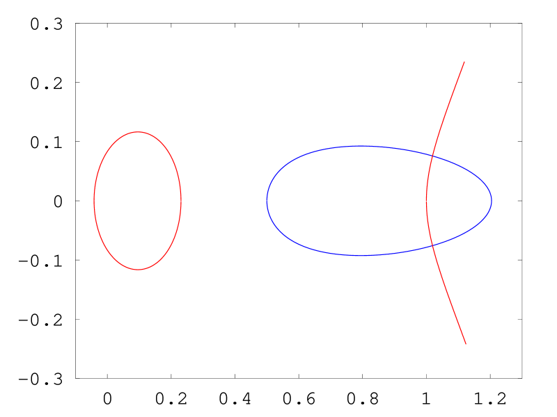
Figure 3:    $\beta_{1}(e^{i\theta})$, $\sqrt{\Delta(e^{i\theta})}$ and a section of $\beta_{2}(e^{i\theta})$ (intersecting $\sqrt{\Delta}$), $\theta\in[0,2\pi)$, on the ${\mathbb{C}}$-plane for the $p$ listed in (45)

Proposition 4.4 extends to $|\alpha|=1$ as follows:

Proposition 4.7.

$${\mathbb{E}}_{z}\left[\exp(i\theta{Z_{\tau}(2))}1_{\{\tau<\infty\}}\right]=\exp(i\theta z(2))\left(\beta_{1}(e^{i\theta})\right)^{z(1)-z(2)}.$$ (62)

and

$$\left|\beta_{1}(e^{i\theta})\right|=\left|{\mathbb{E}}_{(1,0)}\left[\exp(i\theta{Z_{\tau}(2))}1_{\{\tau<\infty\}}\right]\right|\leq r.$$ (63)

Proof.

The dominated convergence theorem implies that

$$\theta\rightarrow{\mathbb{E}}_{z}\left[\exp(i\theta{Z_{\tau}(2)}1_{\{\tau<\infty\}}\right]$$ (64)

is continuous in $\theta$. Proposition 4.1 implies that for each fixed $\theta$ the value of this function equals either

$$\exp(i\theta z(2))\left(\beta_{1}\left(e^{i\theta}\right)\right)^{z(1)-z(2)}$$ (65)

or

$$\exp(i\theta z(2))\left(\beta_{2}\left(e^{i\theta}\right)\right)^{z(1)-z(2)}.$$

(58) and (61) imply that these two expressions are continuous as functions of $\theta$ and they are never equal. Then (64) must equal one or the other for all $\theta$ and therefore if one can verify that (62) equals (65) for a single $\theta$ then the equality must hold for all $\theta$; (54) asserts the desired equality at $\theta=1$; (62) follows. Set $z=(1,0)$ in (62) and take absolute values of both sides:

$$\left|\beta_{1}(e^{i\theta})\right| =\left|{\mathbb{E}}_{(1,0)}\left[\exp(i\theta{Z_{\tau}(2))}1_{\{\tau<\infty\}}\right]\right|$$

$$|\cdot|$$ is convex; then Jensen’s inequality gives

$$\leq{\mathbb{E}}_{(1,0)}\left[1_{\{\tau<\infty\}}\right]=r,$$

where the last equality is (54) with $z(1)=1$. ∎

For two tandem queues, the narrow shaded region of Figure 4 (let’s call it ${\mathcal{R}}$) shows the set of parameter values that violate (56) (the shaded triangle containing ${\mathcal{R}}$ shows the parameter values of stable tandem walks, i.e., the region $\lambda<\mu_{1},\mu_{2}$ where $\lambda=1-\mu_{1}-\mu_{2}$).

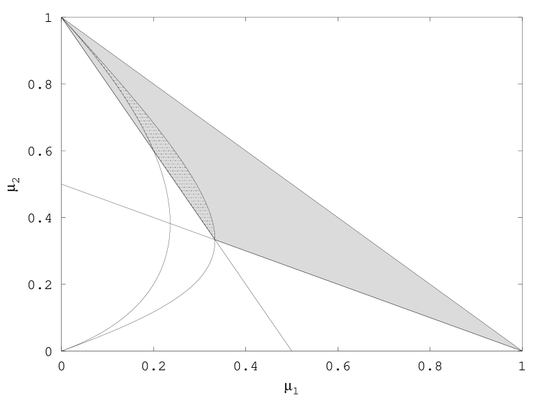
Figure 4:    The set of parameter values violating (56) for the two dimensional tandem walk (the narrow shaded region on the left)

The image of $\theta\rightarrow\Delta(e^{i\theta})$, $\theta\in[0,2\pi)$, becomes a self intersecting curve on ${\mathbb{C}}$ when (56) fails and, e.g., the proof of Proposition 4.5 (or that of its adaptation to the parameter values in ${\mathcal{R}}$) will require a study of $\Re(\Delta)$ over ${\mathcal{R}}$; we leave this analysis to future work.

4.4 $\log$-linear harmonic functions of $Y$

Let us rewrite (35) separately for the boundary $\partial_{2}$ and the interior $B^{o}-\partial_{2}$:

$$V(y) =\sum_{v\in{\mathcal{V}}}V(y+v)p(v),y\in B^{o}-\partial_{2},$$ (66)

$$V(y) =V(y)\mu_{2}+\sum_{v\in{\mathcal{V}},v(2)\neq-1}V(y+v)p(v),y\in\partial_{2}\cap B^{o}.$$ (67)

Any $g\in{\mathcal{F}}_{Z}$ satisfies (66) (because (66) is the restriction of (39) to $B^{o}-\partial_{2}$); (66) is linear and so any finite linear combination of members of ${\mathcal{F}}_{Z}$ continues to satisfy (66). In the next two subsections we will show that appropriate linear combinations of members of ${\mathcal{F}}_{Z}$ will also satisfy the boundary condition (67) and define harmonic functions of $Y$.

Parallel to the definitions in the previous section, we will define characteristic polynomials and surfaces for $Y$. The constrained process will have a pair of these, one set for the interior and one set for the boundary $\partial_{2}$. The interior characteristic polynomial for $Y$ is by definition that of $Z$, i.e., ${\mathbf{p}}$ and its interior characteristic surface is ${\mathcal{H}}$. The characteristic polynomial of $Y$ and its characteristic surface on the boundary $\partial_{2}$ are defined below.

4.4.1 A single term

Remember that members of ${\mathcal{F}}_{Z}$ are of the form $[(\beta,\alpha),\cdot]:z\rightarrow\beta^{z(1)-z(2)}\alpha^{z(2)}$ and $(\beta,\alpha)\in{\mathcal{H}}$; these define harmonic functions for $Z$ and they therefore satisfy (66). The simplest approach of constructing a $Y$-harmonic function is to look for $[(\beta,\alpha),\cdot]$ which satisfies (35), i.e., which satisfies (66) and (67) at the same time. Substituting $[(\beta,\alpha),\cdot]$ in (67) we see that it solves (67) if and only if $(\beta,\alpha)\in{\mathcal{H}}$ also satisfies

$${\mathbf{p}}_{2}(\beta,\alpha)-\beta\alpha=0$$ (68)

where

$${\mathbf{p}}_{2}(\beta,\alpha) \doteq\beta\alpha\left(\sum_{v\in{\mathcal{V}},v(2)\neq-1}p(v)\beta^{v(1)-v(2)}\alpha^{v(2)}+\mu_{2}\right).$$ (69)

We will call (68) “the characteristic equation of $Y$ on $\partial_{2}$” and ${\mathbf{p}}_{2}$ its characteristic polynomial on the same boundary. ${\mathbf{p}}_{2}$ can be expressed in terms of ${\mathbf{p}}$ as follows:

$${\mathbf{p}}_{2} ={\mathbf{p}}(\beta,\alpha)-\beta\alpha\left(\sum_{v\in{\mathcal{V}},v(2)=-1}p(v)\beta^{v(1)-v(2)}\alpha^{v(2)}-\mu_{2}\right)$$

$$={\mathbf{p}}(\beta,\alpha)-\beta\alpha\left(p(2,0)\frac{\beta}{\alpha}+p(2,1)\frac{1}{\alpha}-\mu_{2}\right).$$ (70)

Define the boundary characteristic surface of $Y$ for $\partial_{2}$ as ${\mathcal{H}}_{2}\doteq\{(\beta,\alpha)\in{\mathbb{C}}^{2}:{\mathbf{p}}_{2}(\beta,\alpha)=0\}$.

Then, $(\beta,\alpha)$ must lie on ${\mathcal{H}}\cap{\mathcal{H}}_{2}$ for $[(\beta,\alpha),\cdot]$ to be a harmonic function of $Y$. Suppose $(\beta,\alpha)\in{\mathcal{H}}\cap{\mathcal{H}}_{2}$, i.e., ${\mathbf{p}}_{2}(\beta,\alpha)={\mathbf{p}}(\beta,\alpha)=\beta\alpha$; and $\beta,\alpha\neq 0$. Then, by (70)

$$0 =p(2,1)\frac{1}{\alpha}+p(2,0)\frac{\beta}{\alpha}-\mu_{2},$$

$$\beta =\frac{1}{p(2,0)}\left(\mu_{2}\alpha-p(2,1)\right).$$ (71)

Substituting this back in (44) implies that $\alpha$ must solve

$${\mathbf{p}}^{r}_{2}(\alpha)=0,$$

where

$${\mathbf{p}}^{r}_{2}(\alpha)\doteq\alpha\Bigg{(}\frac{\mu_{2}}{p(2,0)}\left(\mu_{2}\frac{p(1,0)}{p(2,0)}+p(1,2)\right)\alpha^{2}$$

$$~{}~{}+\left(p(0,2)+\frac{\mu_{2}}{p(2,0)}\left(\mu_{2}-2\frac{p(1,0)p(2,1)}{p(2,0)}-1\right)-\frac{p(1,2)p(2,1)}{p(2,0)}\right)\alpha$$

$$~{}~{}~{}+p(0,1)+\frac{p(2,1)}{p(2,0)}\left(1+\frac{p(1,0)p(2,1)}{p(2,0)}-\mu_{2}\right)\Bigg{)};$$

(the superscript $r$ stands for “reduced.”) Then $[(\beta,\alpha),\cdot]$ is a harmonic function of $Y$ if and only if $\alpha$ is a root of ${\mathbf{p}}^{r}_{2}$ and $\beta$ is defined by (71). The functions $z\rightarrow 1$ and $z\rightarrow 0$ are harmonic functions of $Y$ of the form $z\rightarrow\beta^{z(1)-z(2)}\alpha^{z(1)}$; then two of the roots of ${\mathbf{p}}^{r}_{2}$ are $0$ and $1$ (that $0$ is a root also directly follows from the form of ${\mathbf{p}}^{r}_{2}$). It follows that the third root is

$$r_{1}\doteq\frac{p(0,1)+\frac{p(2,1)}{p(2,0)}\left(1+\frac{p(1,0)p(2,1)}{p(2,0)}-\mu_{2}\right)}{\frac{\mu_{2}}{p(2,0)}\left(\mu_{2}\frac{p(1,0)}{p(2,0)}+p(1,2)\right)}.$$

This quantity is always less than $1$ if the first queue is stable:

Lemma 1.

$\nu_{1}<\mu_{1}$ if and only if $r_{1}<1$.

Proof.

$r_{1}<1$ is equivalent to

$$p(0,1)+\frac{p(2,1)}{p(2,0)}(1-\mu_{2}) <p(1,0)+\frac{2p(2,1)p(1,0)}{p(2,0)}+p(1,2)+\frac{p(2,1)p(1,2)}{p(2,0)}$$

substitute $$\mu_{1}+p(0,1)+p(0,2) 1-\mu_{2} p(2,0)$$ for , multiply both sides by and cancel out equal terms from both sides:

$$\mu_{2}p(0,1)+p(2,1)p(0,2) <\mu_{1}p(2,0)+p(2,1)p(1,0)$$ (72)

$$\mu_{2}p(0,1)+p(2,1)p(0,2) <p(1,2)p(2,0)+\mu_{2}p(1,0)$$

$$p(0,1)+\frac{p(2,1)}{\mu_{2}}p(0,2) <p(1,2)\frac{p(2,0)}{\mu_{2}}+p(1,0);$$

divide both sides by $1-\frac{p(1,2)p(2,1)}{\mu_{1}\mu_{2}}$ to get $\nu_{1}<\mu_{1}$. This establishes the “only if” part of the statement of the lemma. The last sequence of inequalities in reverse gives the “if” part. ∎

And thus we get our first nontrivial harmonic function for $Y$:

Proposition 4.8.

The function

$$z\rightarrow\beta(r_{1})^{z(1)-z(2)}r_{1}^{z(1)}$$ (73)

is a harmonic function of $Y$ where

$$\beta(\alpha)\doteq\frac{1}{p(2,0)}\left(\mu_{2}\alpha-p(2,1)\right)$$

is the right side of (71). Furthermore $0<\beta(r_{1})<1$.

Proof.

It remains only to prove the last part of the proposition’s statement. $r_{1}<1$ implies $r_{1}\mu_{2}<\mu_{2}=p(2,0)+p(2,1)$ or, what is the same,

$$\frac{1}{p(2,0)}\left(r_{1}\mu_{2}-p(2,1)\right)<1;$$

this is $\beta(r_{1})<1$. The inequality $\beta(r_{1})>0$ turns out to be true for all $p$ as long as $p(2,0)>0$ and follows from a sequence of inequalities similar to (4.4.1). ∎

4.4.2 Two terms

Define the boundary operator $D_{2}$ acting on functions on ${\mathbb{Z}}^{2}$ and giving functions on $\partial_{2}$:

$$D_{2}V=g,~{}~{}~{}~{}V:{\mathbb{Z}}^{2}\rightarrow{\mathbb{C}},$$

$$g({\mathrm{y}},0)\doteq\left(\mu_{2}+\sum_{v\in{\mathcal{V}},v(2)\neq-1}p(v)V(({\mathrm{y}},0)+v)\right)-V({\mathrm{y}},0),~{}~{}{\mathrm{y}}\in{\mathbb{Z}};$$

(if $V$ is defined on a subset of ${\mathbb{Z}}^{2}$ one may extend it trivially to all of ${\mathbb{Z}}^{2}$ to apply $D_{2}$). $D_{2}$ is the difference between the left and the right sides of (67) and gives how much $V$ deviates from being $Y$-harmonic along the boundary $\partial_{2}$:

Lemma 2.

$D_{2}V=0$ if and only if $V$ is a harmonic function of $Y$ on $\partial_{2}$.

The proof follows from the definitions involved. For $(\beta,\alpha)\in{\mathbb{C}}^{2}$ and $\beta,\alpha\neq 0$

$$\left[D_{2}\left([({\beta,\alpha}),\cdot]\right)\right]({\mathrm{y}},0)=\left(\frac{1}{\beta\alpha}{\mathbf{p}}_{2}(\beta,\alpha)-1\right)\beta^{{\mathrm{y}}}.$$

where the left side denotes the value of the function $D_{2}\left([(\beta,\alpha),\cdot]\right)$ at $({\mathrm{y}},0)$, ${\mathrm{y}}\in{\mathbb{Z}}$. For $(\beta,\alpha)\in{\mathcal{H}}$, ${\mathbf{p}}(\beta,\alpha)=\beta\alpha$; this, the last display and (70) imply

$$\left[D_{2}\left([(\beta,\alpha),\cdot]\right)\right]({\mathrm{y}},0)=\left(\mu_{2}-\left(p(2,0)\frac{\beta}{\alpha}+p(2,1)\frac{1}{\alpha}\right)\right)\beta^{{\mathrm{y}}}$$ (74)

if $(\beta,\alpha)\in{\mathcal{H}}$. One can write the function $({\mathrm{y}},0)\rightarrow\beta^{{\mathrm{y}}}$ as $[(\beta,\alpha),\cdot]|_{\partial_{2}}=[(\beta,1),\cdot]|_{\partial_{2}}$; in addition, define

$$C(\beta,\alpha)\doteq\mu_{2}-\left(p(2,0)\frac{\beta}{\alpha}+p(2,1)\frac{1}{\alpha}\right).$$ (75)

With these, rewrite (74) as

$$D_{2}\left([(\beta,\alpha),\cdot]\right)=C(\beta,\alpha)[(\beta,1),\cdot]|_{\partial_{2}}.$$ (76)

The key observation here is this: $D_{2}\left([(\beta,\alpha),\cdot]\right)$ is a constant multiple of $[(\beta,1),\cdot]|_{\partial_{2}}$. This and the linearity of $D_{2}$ imply that for

$$\alpha_{1}\neq\alpha_{2},~{}~{}(\beta,\alpha_{1}),(\beta,\alpha_{2})\in{\mathcal{H}},$$ (77)

$[(\beta,\alpha_{1}),\cdot]$ and $[(\beta,\alpha_{2}),\cdot]$ can be linearly combined to cancel out each other’s value under $D_{2}$. We will call $(\beta,\alpha_{1})$ and $(\beta,\alpha_{2})$ conjugate if they satisfy (77). An example: the two end points of the dashed line in Figure 2 are conjugate to each other.

Because the characteristic equation (44) is quadratic in $\alpha$, fixing $\beta$ in (44) and solving for $\alpha$ will give a conjugate pair $(\beta,\alpha_{1})$ and $(\beta,\alpha_{2})$ satisfying

$$\alpha_{1}+\alpha_{2}=\frac{\beta-p(1,0)\beta^{2}-p(0,1)}{p(0,2)+\beta p(1,2)}$$ (78)

for most $\beta\in{\mathbb{C}}$; the next proposition uses these conjugate pairs and the above observation to define harmonic functions of $Y$:

Proposition 4.9.

Suppose that for $\beta\in{\mathbb{C}}$, $\beta\neq 0$, $p(0,2)+\beta p(1,2)\neq 0$. Then

$$h_{\beta}\doteq C(\beta,\alpha_{2})[(\beta,\alpha_{1}),\cdot]-C(\beta,\alpha_{1})[(\beta,\alpha_{2}),\cdot]$$ (79)

is a harmonic function of $Y$.

Proof.

By assumption $(\beta,\alpha_{1}),(\beta,\alpha_{2})$ are both on ${\mathcal{H}}$ and therefore $[(\beta,\alpha_{1}),\cdot]$ and $[(\beta,\alpha_{2}),\cdot]$ are harmonic functions of $Z$ and in particular, they both satisfy (66). Then their linear combination $h_{\beta}$ also satisfies (66), because (66) is linear in $V$. It remains to show that $h_{\beta}$ solves (67) as well. $\beta\neq 0$ implies $\alpha_{1},\alpha_{2}\neq 0,1$. Then (76) implies

$$D_{2}(h_{\beta}) =C(\beta,\alpha_{2})D_{2}([(\beta,\alpha_{1}),\cdot])-C(\beta,\alpha_{1})D_{2}([\beta,\alpha_{2},\cdot])$$

$$=C(\beta,\alpha_{2})C(\beta,\alpha_{1})[(\beta,1),\cdot]|_{\partial_{2}}-C(\beta,\alpha_{1})C(\beta,\alpha_{2})[(\beta,1),\cdot]|_{\partial_{2}}$$

$$=0$$

and Lemma 2 implies that $h_{\beta}$ satisfies (67). ∎

Remark 4.

If we set $\beta=\beta(r_{1})$ in the last proposition $h_{\beta}$ reduces to a constant multiple of (73).

With Proposition 4.9 we define our basic class of harmonic functions of $Y$:

$${\mathcal{F}}_{Y}\doteq\{h_{\beta},\beta\neq 0,p(0,2)+\beta p(1,2)\neq 0\}.$$ (80)

Members of ${\mathcal{F}}_{Y}$ consist of linear combinations of $\log$-linear functions; with a slight abuse of language, we will also refer to such functions as $\log$-linear.

Lemma 3.

Suppose $p(0,2)+\beta p(1,2)\neq 0$ so that (78) makes sense. Suppose further that $(\beta,\alpha_{1})\in{\mathcal{H}}$, $(\beta,\alpha_{2})\in{\mathcal{H}}$ are conjugate with $\alpha_{1},\alpha_{2}\neq 0$. Then (78) is equivalent to

$$\alpha_{i}=\frac{1}{\alpha_{3-i}}\frac{p(2,0)\beta^{2}+p(2,1)\beta}{p(0,2)+\beta p(1,2)},i\in\{1,2\}.$$ (81)

Proof.

By (78)

$$\alpha_{i} =\frac{\alpha_{3-i}(\beta-p(1,0)\beta^{2}-p(0,1))}{\alpha_{3-i}(p(0,2)+\beta p(1,2))}-\alpha_{3-i}$$

$$=\frac{\alpha_{3-i}\beta-p(1,0)\beta^{2}-p(0,1)-\alpha_{1}^{2}p(0,2)-\beta\alpha_{3-i}^{2}p(1,2)}{\alpha_{3-i}(p(0,2)+\beta p(1,2))}$$

$$(\alpha_{3-i},\beta)\in{\mathcal{H}}$$ implies

$$=\frac{1}{\alpha_{3-i}}\frac{p(2,0)\beta^{2}+p(2,1)\beta}{p(0,2)+\beta p(1,2)}.$$

∎

Define

$$\boldsymbol{\alpha}(\beta,\alpha)\doteq\frac{1}{\alpha}\frac{p(2,0)\beta^{2}+p(2,1)\beta}{p(0,2)+\beta p(1,2)}$$ (82)

We can write (81) as

$$\alpha_{i}=\boldsymbol{\alpha}(\alpha_{3-i}).$$

The map ${\boldsymbol{\alpha}}$ is invertable (it is a multiple of $\alpha^{-1}$) and its inverse equals itself. Thus, conjugacy is symmetric: if $(\beta,\alpha_{2})$ is conjugate to $(\beta,\alpha_{2})$, then $(\beta,\alpha_{1})$ is conjugate to $(\beta,\alpha_{2})$. We will sometimes refer to $\boldsymbol{\alpha}$ as conjugator.

4.5 Graph representation of $\log$-linear harmonic functions of $Y$

Figure 5 gives a graph representation of the harmonic functions developed in the last subsection.

Figure 5:    The harmonic functions of $Y$

Each node in this figure represents a member of ${\mathcal{F}}_{Z}$. The edges represent the boundary conditions; in this case there is only one, (67) of $\partial_{2}$, and the edge label “$2$” refers to $\partial_{2}$. A self connected vertex represents a member of ${\mathcal{F}}_{Z}$ that also satisfies the $\partial_{2}$ boundary condition (67), i.e., $z\rightarrow\beta(r_{1})^{z(1)}r_{1}^{z(1)-z(2)}$ of Proposition 4.8; the graph on the left represents exactly this function. The “$2$” labeled edge on the right represents the conjugacy relation (81) between $\alpha_{1}$ and $\alpha_{2}$, which allows these functions to be linearly combined to satisfy the harmonicity condition of $Y$ on $\partial_{2}$.

4.6 $\partial B$-determined harmonic functions of $Y$

Our task now is to distinguish a collection of $\partial B$-determined members of ${\mathcal{F}}_{Y}.$ This collection will form a basis of harmonic functions with which we will approximate/ represent the rest of the $\partial B$-determined functions of $Y$.

Proposition 4.10.

Let $\alpha_{1}$, $\alpha_{2}$ and $\beta$ be as in Proposition 4.9. If

$$|\beta|<1,~{}~{}~{}|\alpha_{1}|,|\alpha_{2}|\leq 1$$ (83)

then $h_{\beta}$ of (79) is $\partial B$-determined.

Proof.

By Proposition 4.9 $h_{\beta}$ is a $Y$-harmonic function; (83) and its definition (79) imply that $h_{\beta}$ is also bounded on $B^{o}$. Then $M_{k}=h_{\beta}(Y_{\tau\wedge\zeta_{n}\wedge k})$ is a bounded martingale. This, Proposition 2.2 and the optional sampling theorem imply

$$h_{\beta}(y) ={\mathbb{E}}_{y}\left[h_{\beta}(Y_{\tau})1_{\{\tau<\zeta_{n}\}}\right]+{\mathbb{E}}_{y}\left[h_{\beta}(Y_{\zeta_{n}})1_{\{\zeta_{n}\leq\tau\}}\right],y\in B^{o}.$$ (84)

$Y_{\zeta_{n}}(1)=n$ for $\tau>\zeta_{n}.$ This and (83) imply

$$\lim_{n\rightarrow\infty}{\mathbb{E}}_{y}\left[h_{\beta}(Y_{\zeta_{n}})1_{\{\zeta_{n}\leq\tau\}}\right]\leq\lim_{n\rightarrow\infty}\beta^{n}=0.$$

This, $\lim_{n}\zeta_{n}=\infty$ and letting $n\rightarrow\infty$ in (84) give

$$h_{\beta}(y)={\mathbb{E}}_{y}\left[h_{\beta}(Y_{\tau})1_{\{\tau<\infty\}}\right],$$

i.e, $h_{\beta}$ is $\partial B$-determined. ∎

Remark 4, Proposition 4.8 and the last proposition imply

Proposition 4.11.

The harmonic function (73) is $\partial B$-determined.

What Proposition 4.10 does is it gives us a collection of basis functions for which the Balayage operator ${\mathcal{T}}_{(B^{o})^{c}}$ is extremely simple to compute; these functions play the same role for the current problem as the one which exponential functions do in the solution of linear ordinary differential equations or the trigonometric functions in the solution of the heat and the Laplace equations. Let us rewrite Proposition 4.10 more explicitly. Suppose $\alpha_{1}$, $\alpha_{2}$ and $\beta$ are as in Proposition 4.10. Define

$$f(y)=C(\beta,\alpha_{2})\alpha_{1}^{y(2)}-C(\beta,\alpha_{1})\alpha_{2}^{y(2)},y\in{\mathbb{Z}}^{2}.$$

Then, Proposition 4.10 says

$${\mathbb{E}}_{y}\left[f(Y_{\tau})1_{\{\tau<\infty\}}\right] =\beta^{y(1)-y(2)}\left(C(\beta,\alpha_{2})\alpha_{1}^{y(2)}-C(\beta,\alpha_{1})\alpha_{2}^{y(2)}\right)$$

$$=\beta^{y(1)-y(2)}f(y),~{}~{}~{}y\in B.$$

Proposition 4.10 rests on the condition (83); Proposition 4.13 below identifies a set of conjugate pairs $(\beta,\alpha_{1})$ and $(\beta,\alpha_{2})$ on ${\mathcal{H}}$ satisfying (83).

4.7 A modified Fourier basis for ${\mathcal{T}}_{(B^{o})^{c}}$

Let’s go back for a moment to the problem of evaluating the Balayage operator of the unconstrained process $Z$ for the set $(B_{Z}^{o})^{c}$. For a bounded function $f$ on $\partial B_{Z}$, this is the operator mapping $f$ to the harmonic function

$${\mathcal{T}}_{(B_{Z}^{o})^{c}}(f)=z\rightarrow{\mathbb{E}}_{z}\left[f(Z_{\tau})1_{\{\tau<\infty\}}\right],z\in B_{Z};$$

in the present subsection we will write ${\mathcal{T}}$ for ${\mathcal{T}}_{(B_{Z}^{o})^{c}}$ For the Fourier basis functions

$$f_{\alpha}:\partial B_{Z}\rightarrow{\mathbb{C}},f_{\alpha}({\mathrm{y}},{\mathrm{y}})=\alpha^{y},{\mathrm{y}}\in{\mathbb{Z}},|\alpha|=1,$$ (85)

we already know how to compute ${\mathcal{T}}(f_{\alpha})$ (given by (62)) and ${\mathcal{T}}$ is linear. One can use these to evaluate ${\mathcal{T}}$ more generally in three related ways. First, Fourier series theory tells us that if $f$ is $l_{2}$, i.e., if $\sum_{{\mathrm{y}}\in{\mathbb{Z}}}|f({\mathrm{y}},{\mathrm{y}})|^{2}<\infty$, it can be written in terms of the Fourier basis functions thus:

$$f({\mathrm{y}},{\mathrm{y}})=\frac{1}{2\pi}\int_{-\pi}^{\pi}\hat{f}(\theta)e^{i{\mathrm{y}}\theta}d\theta,\hat{f}(\theta)\doteq\sum_{{\mathrm{y}}=-\infty}^{\infty}f({\mathrm{y}},{\mathrm{y}})e^{-i{\mathrm{y}}\theta}$$ (86)

Fubini’s theorem now implies ${\mathcal{T}}(f)=\frac{1}{2\pi}\int_{-\pi}^{\pi}\hat{f}(\theta){\mathcal{T}}(f_{e^{i\theta}})d\theta$, and one can construct approximating sequences by truncating the sum in (86).

Second, when interpreted as a function of $\alpha$, the formula (62) gives the characteristic function of the distribution ${\mathcal{T}}$. Its inversion would give the distribution ${\mathcal{T}}$ itself.

Third, we can first replace $f$ with its periodic approximation defined as follows

$$f^{p}({\mathrm{y}},{\mathrm{y}})=\begin{cases}f({\mathrm{y}},{\mathrm{y}}),\text{ if }|{\mathrm{y}}|\leq N,\\ f({\mathrm{y}}\mod N,{\mathrm{y}}\mod N),\text{ if }|{\mathrm{y}}|\geq N.\end{cases}$$

As $N$ increases, $|{\mathcal{T}}(f^{p})-{\mathcal{T}}(f)|$ will converge to $0$. Because it is periodic, $f^{p}$ has a unique Fourier representation of the form $f^{p}=\sum_{k=0}^{2N+1}c_{k}f_{\alpha_{k}}$ where $\alpha_{k}=e^{i\left(\frac{k2\pi}{2N+1}\right)}.$ Then ${\mathcal{T}}(f^{p})=\sum_{k=0}^{2N+1}c_{k}{\mathcal{T}}(f_{\alpha_{k}}).$

How should one proceed to build a parallel theory for the constrained process $Y$? The first obstacle to the above development in the case of $Y$ is that the Balayage of the Fourier basis functions is not simple to compute, i.e., we don’t know a simple way to compute ${\mathcal{T}}_{(B^{o})^{c}}(f_{\alpha})$. But Proposition 4.10 says that if

$$|\alpha^{\prime}={\boldsymbol{\alpha}}(\beta_{1}(\alpha),\alpha)|<1,~{}~{}C(\beta_{1}(\alpha),\alpha^{\prime})\neq 0$$ (87)

then the Balayage of the perturbed Fourier basis function

$$({\mathrm{y}},{\mathrm{y}})\rightarrow\alpha^{\mathrm{y}}-\frac{C(\beta_{1}(\alpha),\alpha)}{C(\beta_{1}(\alpha),\alpha^{\prime})}(\alpha^{\prime})^{\mathrm{y}},{\mathrm{y}}\in{\mathbb{Z}}_{+},$$ (88)

is simple to compute and is given by

$$y\rightarrow\beta_{1}(\alpha)^{y(1)-y(2)}\left(\alpha^{y(2)}-\frac{C(\beta_{1}(\alpha),\alpha)}{C(\beta_{1}(\alpha),\alpha^{\prime})}(\alpha^{\prime})^{y(2)}\right),y\in B.$$ (89)

One can interpret (88) as a perturbation of the restriction of (85) to $\partial B$, because $|\alpha^{\prime}|<1$ implies that these two functions equal each other for ${\mathrm{y}}$ large. Below in Proposition 4.13 we identify a set of $\alpha$’s for which (87) holds and, therefore, for which the image of (88) under the Balayage operator is given by (89). This will require further assumptions on $p$; in particular, we will assume (87) for $\alpha=1$:

$${\boldsymbol{\alpha}}(r,1)<1,$$ (90)

$$C(r,{\boldsymbol{\alpha}}(r,1))\neq 0,$$ (91)

where, as before, $r$ is the input/output ratio (17).

Comments on these assumptions:

1. If $p(2,1)$ is large enough, ${\boldsymbol{\alpha}}(r,1)$ can exceed $1$ even when the stability assumption (14) holds. For such networks, we cannot check whether $h_{r}$ is $\partial B$-determined by an application of Proposition 4.10. Furthermore, even if $h_{r}$ is $\partial B$-determined, $[(r,{\boldsymbol{\alpha}}(r,1)),\cdot]$ will dominate $h_{r}$ for large $y(2)$ and one can no longer think of $h_{r}/C(r,{\boldsymbol{\alpha}}(r,1))$ as a perturbation of the function $1$ on $\partial B$.

2. The condition (91) implies that the $\log$-linear function $[(r,{\boldsymbol{\alpha}}(r,1)),\cdot]$ is not $Y$-harmonic. For two dimensional tandem walk, (91) reduces to $\mu_{1}\neq\mu_{2}$. One can treat the case $\mu_{1}=\mu_{2}$ by writing it as the limit $\mu_{1}\rightarrow\mu_{2}$. This limiting procedure introduces harmonic functions with polynomial terms, see subsection 9.4.

With (90) and (91) we are able to take $\alpha=1$ in (88). Subsection 4.4.1 implies that for $\alpha\in S^{1}$ and $\alpha\neq 1$, $C(\beta_{1}(\alpha),\alpha)\neq 0$. Thus, for such $\alpha$ only the first condition in (87) is nontrivial. In the next proposition we will show that (90) implies $|\boldsymbol{\alpha}(\beta_{1}(\alpha),\alpha)|<1$ for all $|\alpha|=1$. To simplify its proof, we will further assume $p(0,2)=0.$ Treating $p(0,2)\neq 0$ seems to require a more refined analysis of $\beta_{1}$ as a function of $p$ and $\alpha$, a task we defer to future work.

Proposition 4.12.

Suppose $p(0,2)=0$, (90) and (52) hold; for $p(1,2)=0$ the system becomes trivial, so we will also assume $p(1,2)\neq 0.$ Then

$$|{\boldsymbol{\alpha}}(\beta_{1}(\alpha),\alpha)|<1$$ (92)

for all $|\alpha|=1$.

Proof.

The definition of ${\boldsymbol{\alpha}}$ and $p(0,2)=0$ imply ${\boldsymbol{\alpha}}(\beta,\alpha)={\bf c}(\alpha)/\alpha$ where

$${\bf c}(\alpha)\doteq(p(2,0)\beta_{1}(\alpha)+p(2,1))/p(1,2).$$

Then

$$|{\boldsymbol{\alpha}}(\beta_{1}(\alpha),\alpha)|=|{\bf c}(\alpha)|$$ (93)

because $|\alpha|=1$. As $\alpha$ varies on $S^{1}$, ${\bf c}(\alpha)$ defines a closed curve in ${\mathbb{C}}$ that is symmetric around the real axis. (63) implies that this curves is contained in a circle centered at the point $p(2,1)/p(1,2)$ with radius $rp(2,0)/p(1,2)$, which in turn is contained in the circle centered at the origin and with radius $(p(2,1)+rp(2,0))/p(1,2)={\boldsymbol{\alpha}}(r,1)$ which by assumption (90) is less than $1$; then $|{\bf c}(\alpha)|<1$. This and (93) imply (92). ∎

We have assumed $p(0,2)=0$ only to simplify the above proof; Figure 6 shows an example with $p(2,0)\neq 0$ where again $|\boldsymbol{\alpha}|<1$.

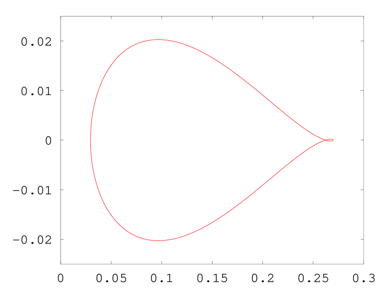
Figure 6:    The graph of ${\boldsymbol{\alpha}}(\beta,\alpha)$, $\alpha=\exp(i\theta)$ on the ${\mathbb{C}}$-plane as $\theta$ varies in $[0,2\pi)$ for the $p$ of (45)

Remark 5.

If $p(2,0)/p(1,0)=1$, $\alpha=-1$ violates (52) and the last proposition is not applicable at $\alpha=-1$, because $\beta_{1}$ is not well defined there. But in that case the single root of the affine (46) will take the place of $\beta_{1}$ above. With this modification, the above argument works verbatim for $p(2,0)/p(1,0)=1$ as when $p(2,0)/p(1,0)\neq 1$ and from here on we assume that a similar modification is made when a violation of (52) occurs.

Proposition 4.13.

Assume (14), (90), (91) and (56). Then there exists $0<R<1$ such that for all $\alpha\in{\mathbb{C}}$ with $R<|\alpha|\leq 1$, $h_{\beta_{1}(\alpha)}$ is a $\partial B$-determined harmonic function of $Y$.

Proof.

Proposition 4.10 and Proposition 4.12 imply that $h_{\beta_{1}(\alpha)}$ is $\partial B$-determined harmonic function of $Y$ for $\alpha\in S^{1}.$ $\boldsymbol{\alpha}$ and $\beta_{1}$ are continuous functions. This, compactness of $S^{1}$ and (63) imply

$$|\beta_{1}(\alpha)|,|\boldsymbol{\alpha}(\beta_{1}(\alpha),\alpha)|<1$$

for $|\alpha|\in(R,1]$ where $R$ is sufficiently close to $1$. This and Proposition 4.10 now imply the statement of the proposition. ∎

5 Analysis of $Y$, $d>2$

Now we would like to extend some of the ideas of the previous section to $d$ dimensions. Our path will be this: each of the graphs shown in Figure 5 and its corresponding equations define a harmonic function of $Y$. We will develop the graph representation in $d$ dimensions and show that any solution of the equations represented by a certain class of graphs defines a harmonic function of $Y$.

For $\alpha\in{\mathbb{C}}^{d-1}$ we will index the components of the vector $\alpha$ with the set ${\mathcal{N}}\doteq{\mathcal{N}}_{0}-\{0,1\}$, i.e., $\alpha=(\alpha(2),\alpha(3),...,\alpha(d)).$ The members of ${\mathcal{N}}$ are exactly the constrained coordinates of $Y$. For $a\subset{\mathcal{N}}$ the constraining map $\pi$ sets the following set of increments of $Y$ to $0$ on $\partial_{a}$:

$${\mathcal{V}}_{a}\doteq\{v:v\in{\mathcal{V}},v(j)\neq-1,\text{ for }j\in a\}.$$

Rewrite (35) as

$$V(y)=V(y)\sum_{j\in a}\mu_{j}+\sum_{v\in{\mathcal{V}}_{a}}V(y+v)p(v),y\in\partial_{a}\cap O,a\subset{\mathcal{N}}.$$ (94)

Set

$$[(\beta,\alpha),z]\doteq\beta^{z(1)-\sum_{j\in{\mathcal{N}}}z(j)}\prod_{j\in{\mathcal{N}}}\alpha(j)^{z(j)}.$$ (95)

$[(\beta,\alpha),z]$ is $\log$-linear in $z$, i.e., $\log([(\beta,\alpha),z])$ is linear in $z$; our goal is to construct $Y$-harmonic functions out of linear combinations of these functions.

Define the characteristic polynomial

$${\mathbf{p}}_{a}(\beta,\alpha)\doteq\left(\sum_{v\in{\mathcal{V}}_{a}}p(v)[(\beta,\alpha),v]+\sum_{j\in a}\mu_{j}\right)$$ (96)

the characteristic equation

$${\mathbf{p}}_{a}(\beta,\alpha)=1,$$ (97)

and the characteristic surface

$${\mathcal{H}}_{a}\doteq\{(\beta,\alpha)\in{\mathbb{C}}^{d}:{\mathbf{p}}_{a}(\beta,\alpha)=1\}$$ (98)

of the boundary $\partial_{a}$, $a\subset{\mathcal{N}}$. We will write ${\mathbf{p}}$ and ${\mathcal{H}}$ instead of ${\mathbf{p}}_{\emptyset}$ and ${\mathcal{H}}_{\emptyset}.$

Generalize (70) to the current setup as

$${\mathbf{p}}_{a}(\beta,\alpha)={\mathbf{p}}(\beta,\alpha)-\left(\sum_{v\in{\mathcal{V}}_{a}^{c}}p(v)[(\beta,\alpha),v]-\sum_{j\in a}\mu_{j}\right).$$ (99)

${\mathbf{p}}_{a}$ is not a polynomial but a rational function; to make it a polynomial one must multiply it by $\beta\prod_{j\in{\mathcal{N}}}\alpha(j)$; this is what we did when we gave the two dimensional versions of these definitions in (43) and (69). For $d>2$, the $\beta\prod_{j\in{\mathcal{N}}}\alpha(j)$ multiplier complicates notation; for this reason we omit it but continue to refer to the rational (96) as the “characteristic polynomial.”

The argument in subsection 4.4.1 continues to work verbatim for general $d$ and gives

Lemma 4.

Suppose $(\beta,\alpha)\in{\mathcal{H}}\cap{\mathcal{H}}_{i}$. Then $[(\beta,\alpha),\cdot]$ is $Z$-harmonic (i.e., $Y$-harmonic on $\Omega_{Y}^{o}$) and $Y$-harmonic on $\partial_{i}.$

Our next step is to extend the content of subsection 4.4.2 to the current setup. Begin with the operator $D_{a}$ acting on functions on ${\mathbb{Z}}^{d}$ and giving functions on $\partial_{a}$:

$$D_{a}V=g,~{}~{}~{}~{}V:{\mathbb{Z}}^{d}\rightarrow{\mathbb{C}},$$

$$g(z)\doteq\left(\sum_{j\in a}\mu_{a}+\sum_{v\in{\mathcal{V}_{a}}}p(v)V(z+v)\right)-V(z).$$

Lemma 5.

$D_{a}V=0$ if and only if $V$ is $Y$-harmonic on $\partial_{a}$.

The proof follows from the definitions. Next generalize $C$ of (75) to

$$C(j,\beta,\alpha)\doteq\mu_{j}-\sum_{v\in{\mathcal{V}},v(j)=-1}p(v)[(\beta,\alpha),v].$$ (100)

For $\alpha\in{\mathbb{C}}^{{\mathcal{N}}}$ and $a\subset{\mathcal{N}}$ define $\alpha\{a\}\in{\mathbb{C}}^{{\mathcal{N}}}$ as follows: $\alpha\{a\}|_{a^{c}}=\alpha|_{a^{c}}$ and $\alpha\{a\}|_{a}=1$; If $a=\{i\}$, we will write $\alpha\{i\}$, instead of $\alpha\{\{i\}\}.$ For example, for ${\mathcal{N}}=\{2,3,4\}$, $a=\{4\}$ and $\alpha=(0.2,0.3,0.4)$, $\alpha\{a\}=(0.2,0.3,1).$ We will use this notation in the next paragraph, where we define the conjugacy of points on ${\mathcal{H}}$ in $d$ dimensions and in the next section where we apply the results of the present section to $d$-tandem queues.

For $i\in{\mathcal{N}}$, fix $\alpha|_{{\mathcal{N}}-\{i\}}$, $\beta$ and multiply both sides of the characteristic equation (97) by $\alpha(i)$; this gives a second order polynomial equation in $\alpha(i)$. If $\beta$ and $\alpha|_{{\mathcal{N}}-\{i\}}$ are such that the discriminant of this polynomial is nonzero, we get two distinct points $(\beta,\alpha_{1})$ and $(\beta,\alpha_{2})$ on ${\mathcal{H}}$ which satisfy

$$\alpha_{1}|_{{\mathcal{N}}-\{i\}} =\alpha_{2}|_{{\mathcal{N}}-\{i\}},$$ (101)

$$\alpha_{1}(i)+\alpha_{2}(i) =\frac{1-\sum_{v(i)=0}[(\beta,\alpha_{1}),v]}{\sum_{v(i)=1}[(\beta,\alpha_{1}\{i\}),v]}.$$ (102)

The sum in the numerator on the right side of (102) is over $v$ such that $v(i)=0$; this and (101) imply that (102) remains the same if we replace $[(\beta,\alpha_{1}),v]$ in the numerator with $[(\beta,\alpha_{2}),v]$ or $[(\beta,\alpha_{2}\{i\}),v]=[(\beta,\alpha_{1}\{i\}),v]$. Rewrite (102) as

$$\alpha_{2}(i) =\frac{1-\sum_{v(i)=0}[(\beta,\alpha_{1}),v]}{\sum_{v(i)=1}[(\beta,\alpha_{1}\{i\}),v]}-\alpha_{1}(i)$$

$$=\frac{1-\sum_{v(i)=0}[(\beta,\alpha_{1}),v]-\sum_{v(i)=1}[(\beta,\alpha_{1}),v]}{\sum_{v(i)=1}[(\beta,\alpha_{1}\{i\}),v]}$$

$$=\frac{\sum_{v(i)=-1}[(\beta,\alpha_{1}),v]}{\sum_{v(i)=1}[(\beta,\alpha_{1}\{i\}),v]}=\frac{1}{\alpha_{1}(i)}\frac{\sum_{v(i)=-1}[(\beta,\alpha_{1}\{i\}),v]}{\sum_{v(i)=1}[(\beta,\alpha_{1}\{i\}),v]}$$ (103)

Now keep $$\alpha_{2}(i)$$ on the left and repeat the same computation to get

$$\alpha_{1}(i) =\frac{1}{\alpha_{2}(i)}\frac{\sum_{v(i)=-1}[(\beta,\alpha_{2}\{i\}),v]}{\sum_{v(i)=1}[(\beta,\alpha_{2}\{i\}),v]}.$$ (104)

We will call $(\beta,\alpha_{1})\neq(\beta,\alpha_{2})\in{\mathcal{H}}$ $i$-conjugate if they satisfy (101) and any of the equivalent (102), (103) and (104). Based on these, generalize the conjugator ${\boldsymbol{\alpha}}$ as ${\boldsymbol{\alpha}}(i,(\beta,\alpha_{1}))=\alpha_{2}$ where $\alpha_{2}$ is defined by (101) and (103).

Our next proposition generalizes Proposition 4.9 to the current setup. In its proof the, following decomposition, which (99) implies, will be useful:

$$D_{a}([(\beta,\alpha,\cdot)])(z) =\left(\sum_{j\in a}\mu_{j}-\sum_{v\in{\mathcal{V}}_{a}^{c}}p(v)[(\beta,\alpha),v]\right)[(\beta,\alpha),z]$$ (105)

$$=\sum_{j\in a}\left(\mu_{j}-\sum_{v\in{\mathcal{V}},v(j)=-1}p(v)[(\beta,\alpha),v]\right)[(\beta,\alpha),z]$$

$$=\sum_{j\in a}D_{j}([(\beta,\alpha,\cdot)])(z)$$ (106)

for $z\in\partial_{a}$ and $(\beta,\alpha)\in{\mathcal{H}}$.

Proposition 5.1.

Suppose that $(\beta,\alpha_{1})$ and $(\beta,\alpha_{2})$ are $i$-conjugate and $C(i,\beta,\alpha_{j})$, $j=1,2$ are well defined. Then

$$h_{\beta}\doteq C(i,\beta,\alpha_{2})[(\beta,\alpha_{1}),\cdot]-C(i,\beta,\alpha_{1})[(\beta,\alpha_{2}),\cdot]$$

is $Y$-harmonic on $\partial_{i}$.

Proof.

The definition (100) of $C$, (105) and linearity of $D_{i}$ imply

$$D_{i}(h_{\beta}) =C(i,\beta,\alpha_{2})C(i,\beta,\alpha_{1})[(\beta,\alpha_{1}),\cdot]-C(i,\beta,\alpha_{2})C(i,\beta,\alpha_{1})[(\beta,\alpha_{2}),\cdot]$$

(101) implies $$[(\beta,\alpha_{1}),z]=[(\beta,\alpha_{2}),z] z\in\partial_{i}$$ for and therefore the last line reduces to

$$=0.$$

Lemma 5 now implies that $h_{\beta}$ is $Y$-harmonic on $\partial_{i}$. ∎

To generalize the graph representation of the previous section we will need graphs with labeled edges; let us denote any graph by its adjacency matrix $G$. Let $V_{G}$, a finite set, denote the set of vertices of $G$ . Each edge of $G$ will have a label taking values in a finite set $L$. For two vertices $i\neq j$, $G(i,j)=0$ if they are disconnected, and $G(i,j)=l$ if an edge with label $l\in L$ connects them; such an edge will be called an $l$-edge. As usual, an edge from a vertex to itself is called a loop. For a vertex $j\in V_{G}$, $G(j,j)$ is the set of the labels of the loops on $j$. Thus $G(j,j)\subset L$ is set valued.

Definition 5.1.

Let $G$ and $L$ be as above. If each vertex $j\in V_{G}$ has a unique $l$-edge (perhaps an $l$-loop) for all $l\in L$ we will call $G$ edge-complete with respect to $L$.

We say $G$ is edge-complete with respect to $Y$ if it is so with respect to ${\mathcal{N}}={\mathcal{N}}_{0}-\{0,1\}$ (remember that ${\mathcal{N}}$ is the set of constrained coordinates of $Y$). If we just say “edge-complete” we mean “edge-complete with respect to $Y$.”

Definition 5.2.

A $Y$-harmonic system consists of an edge-complete graph $G$ with respect to ${\mathcal{N}}$, the variables $(\beta,\alpha_{j})\in{\mathbb{C}}^{d}$, ${\boldsymbol{c}}_{j}\in{\mathbb{C}}$, $j\in V_{G}$, and these equations/constraints:

1. $(\beta,\alpha_{j})\in{\mathcal{H}},{\boldsymbol{c}}_{j}\in{\mathbb{C}}-\{0\},j\in V_{G}$,

2. $\alpha_{i}\neq\alpha_{j}$, if $i\neq j,i,j\in V_{G}$,

3. $\alpha_{i},\alpha_{j}$ are $G(i,j)$-conjugate if $G(i,j)\neq 0$, $i\neq j,i,j\in V_{G}$,

4. $${\boldsymbol{c}}_{i}/{\boldsymbol{c}}_{j}=-\frac{C(G(i,j),\beta,\alpha_{j})}{C(G(i,j),\beta,\alpha_{i})},\text{ if }G(i,j)\neq 0,$$ (107)

5. $(\beta,\alpha_{j})\in{\mathcal{H}}_{l}\text{ for all }l\in G(j,j),j\in V_{G}.$

Proposition 5.2.

Suppose that a $Y$-harmonic system for and edge-complete $G$ has a solution; then

$$h_{G}\doteq\sum_{j\in V_{G}}{\boldsymbol{c}}_{j}[(\beta,\alpha_{j}),\cdot]$$ (108)

is a harmonic function of $Y$.

Proof.

All summands of $h_{G}$ are $Z$-harmonic and therefore $Y$-harmonic on $\Omega_{Y}^{o}$ because $(\beta,\alpha_{j})$, $j\in V_{G}$, are all on the characteristic surface ${\mathcal{H}}$. It remains to show that $h_{G}$ is $Y$-harmonic on all $\partial_{a}\cap\Omega_{Y}$, $a\subset{\mathcal{N}}$ and $a\neq\emptyset.$ We will do this by induction on $|a|$. Let us start with $|a|=1$, i.e., $a=\{l\}$ for some $l\in{\mathcal{N}}$. Take any vertex $i\in V_{G}$; if $l\in G(i,i)$ then $(\beta,\alpha_{i})\in{\mathcal{H}}_{l}$ and by Lemma 4 $[(\beta,\alpha_{i}),\cdot]$ is $Y$-harmonic on $\partial_{l}$. Otherwise, the definition of a harmonic system implies that there exists a unique vertex $j$ of $G$ such that $G(i,j)=l$. This implies, by definition, that $(\beta,\alpha_{i})$ and $(\beta,\alpha_{j})$ are $l$-conjugate and by Proposition 5.1 and (107)

$${\boldsymbol{c}}_{i}[(\beta,\alpha_{i}),\cdot]+{\boldsymbol{c}}_{j}[(\beta,\alpha_{j}),\cdot]$$

is $Y$-harmonic on $\partial_{l}$. Thus, all summands of $h_{G}$ are either $Y$-harmonic on $\partial_{l}$ or form pairs which are so; this implies that the sum $h_{G}$ is $Y$-harmonic on $\partial_{l}$.

Now assume $h_{G}$ is $Y$-harmonic for all $a^{\prime}$ with $|a^{\prime}|=k-1$; fix $a\subset{\mathcal{N}}$ such that $|a|=k$ and $i\in a$; by (106)

$$D_{a}(h_{G})=D_{a-\{i\}}(h_{G})+D_{i}(h_{G}).$$

The induction assumption and Lemma 5 imply that the first term on the right is zero; the same lemma and the previous paragraph imply the same for the second term. Then $D_{a}(h_{G})=0$; this and Lemma 5 finish the proof of the induction step. ∎

Proposition 5.3.

Let $(\beta,\alpha_{j})$, ${\boldsymbol{c}}_{j}$, $j\in V_{G}$, be the solutions of a $Y$-harmonic system for an edge-complete $G$ and let $h_{\beta}$ be defined as in (108). If

$$|\beta|<1,~{}~{}~{}|\alpha_{j}(i)|\leq 1,~{}~{}i\in{\mathcal{N}},$$

then $h_{G}$ is $\partial B$-determined.

The proof is identical to that of Proposition 4.10.

5.1 Simple extensions

One can build, from the solution of a given harmonic system for $Y$, solutions to related harmonic systems for higher dimensional walks which are, in some natural sense, extensions of $Y$. The construction will depend on what we mean by an “extension.” One possibility is that of a simple extension whose definition follows.

So far, we have taken $p$ to be a $(d+1)\times(d+1)$ real matrix, i.e., $p\in{\mathbb{R}}_{+}^{(d+1)\times(d+1)}$ where $d+1=|{\mathcal{N}}_{0}|$. To define “simple extensions” it is more convenient to take the set of nodes ${\mathcal{N}}_{0}$ to be an arbitrary set with $d+1$ elements containing $0$ and $p\in{\mathbb{R}}_{+}^{{\mathcal{N}}_{0}\times{\mathcal{N}}_{0}}$. ${\mathcal{N}}_{+}$ is, as before, ${\mathcal{N}}_{0}-\{0\}.$ Suppose ${\mathcal{N}}_{0}^{1}\supset{\mathcal{N}}_{0}$ and $p_{1}\in{\mathbb{R}}_{+}^{{\mathcal{N}}_{0}^{1}\times{\mathcal{N}}_{0}^{1}}$ is another matrix of jump probabilities. Define $p^{\prime}\in{\mathbb{R}}_{+}^{{\mathcal{N}}_{0}\times{\mathcal{N}}_{0}}$ as follows

$$p^{\prime}(i,j) =p_{1}(i,j)$$ (109)

if $$i\in{\mathcal{N}}_{0} j\in{\mathcal{N}}_{+}$$, ,

$$p^{\prime}(i,0) =p_{1}(i,0)+\sum_{j\in{\mathcal{N}}_{0}^{1}-{\mathcal{N}}_{0}}p_{1}(i,j).$$ (110)

Definition 5.3.

We say that $p_{1}$ is a simple extension of $p$ if

$$p^{\prime}=\left(\sum_{i,j\in{\mathcal{N}}_{0}}p^{\prime}(i,j)\right)p,p^{\prime}\neq 0,$$ (111)

$$p_{1}(i,j)=0\text{ if }i\in{\mathcal{N}}^{1}_{0}-{\mathcal{N}}_{0}\text{ and }j\in{\mathcal{N}}_{+}.$$ (112)

An example: take ${\mathcal{N}}_{0}=\{0,1,2\}$, ${\mathcal{N}}^{1}_{0}=\{0,1,2,3,4\}$, and

$$p=\left(\begin{matrix}0&1/7&0\\ 0&0&4/7\\ 2/7&0&0\end{matrix}\right),p_{1}=\left(\begin{matrix}0&0.05&0&0&0.02\\ 0&0&0.2&0&0\\ 0.1&0&0&0.1&0\\ 0&0&0&0&0.25\\ 0.1&0&0&0.18&0\end{matrix}\right).$$

Figure 7 shows the topologies of the networks corresponding to $p$ and $p_{1}.$

Figure 7:    Two networks, second is a simple extension of the first

Next define the “edge-complete extension” of a given edge-complete graph:

Definition 5.4.

Let $G$ be an edge-complete graph with respect to a finite label set $L$ . Its edge-complete extension $G_{1}$ with respect to another set of nodes ${L}_{1}\supset L$ is defined as follows: $V_{G_{1}}=V_{G}$ and

$$G_{1}(i,j) =G(i,j),i\neq j,i,j\in V_{G}$$

$$G_{1}(j,j) =G(j,j)\cup(L_{1}-L),j\in V_{G}.$$

To get $G_{1}$ from $G$ one adds to each vertex of $G$ an $l$-loop for each $l\in L_{1}-L$. Then if $G$ is edge-complete with respect to $L$, so must be $G_{1}$ with respect to $L_{1}.$ Figure 8 gives an example.

Figure 8:    An edge-complete graph with respect to $\{2\}$ and its edge-complete extension to $\{2,3,4,5\}$

Suppose $Y^{1}$ is a simple extension of $Y$; the next proposition explains how one can construct harmonic systems (and their solutions) for $Y^{1}$ from those of $Y$.

Proposition 5.4.

Let $Y^{1}$ be another constrained process defined using the construction (22) (in particular $i=1$ and only the first coordinate of $Y^{1}$ is unconstrained and its remaining coordinates are constrained) and such that its matrix of jump probabilities $p_{1}$ is a simple extension of the $p$ matrix of $Y$. Let $G_{1}$ and $G_{0}$ be edge-complete graphs for $Y^{1}$ and $Y$ such that $G_{1}$ is an edge-complete extension of $G_{0}$. Suppose $(\beta,\alpha_{k}),{\boldsymbol{c}}_{k},k\in V_{G_{0}}$, solve the harmonic system associated with $G_{0}$. For $k\in V_{G_{1}}=V_{G_{0}}$ define $\alpha^{1}_{k}$ as follows

$$\alpha^{1}_{k}|_{{\mathcal{N}}} =\alpha_{k},$$ (113)

$$\alpha^{1}_{k}|_{{\mathcal{N}}^{1}-{\mathcal{N}}} =\beta,$$ (114)

where ${\mathcal{N}}^{1}\supset{\mathcal{N}}$ is the set of constrained coordinates of the process $Y^{1}$. Then $(\beta,\alpha^{1}_{k}),{\boldsymbol{c}}_{k},k\in V_{G_{1}}$, solve the harmonic system defined by $G_{1}$.

The definition (114) assigns the value $\beta$ to the new components of $\alpha^{1}_{k}$ coming from the new dimensions of the simple extension; this corresponds to ignoring the new dimensions when we compute the $\log$-linear function $[(\beta,\alpha^{1}_{k}),\cdot]$ at the increments of $Y^{1}$ (see (116) and (117) below). The following proof lays down the details of this observation.

Proof.

Set ${\mathcal{N}}^{1}_{0}={\mathcal{N}}^{1}\cup\{0,1\}$ and ${\mathcal{N}}^{1}_{+}={\mathcal{N}}^{1}\cup\{1\}$. By assumption, $(\beta,\alpha_{k})$, ${\boldsymbol{c}}_{k}$, $k\in V_{G_{0}}$, satisfy the five conditions listed under Definition 5.2 for $G=G_{0}$. We want to show that this implies that the same holds for $(\beta,\alpha^{1}_{k})$, ${\boldsymbol{c}}_{k}$, $k\in V_{G_{1}}$ for $G=G_{1}.$ Let ${\mathcal{V}}^{1}_{0}$ denote the set of increments of $Y^{1}$, $e^{1}_{j}$, $j\in{\mathcal{N}}^{1}_{+}$ the unit functions on ${\mathcal{N}}^{1}_{+}$ and let $e^{1}_{0}$ be the $0$ function on the same set. (112) implies that we can partition ${\mathcal{V}}^{1}_{0}$ as follows:

$${\mathcal{V}}^{1}_{0} ={\mathcal{V}}^{1}_{1}\cup{\mathcal{V}}^{1}_{2}\cup{\mathcal{V}}^{1}_{3},$$ (115)

$${\mathcal{V}}^{1}_{1} \doteq\{e_{1}^{1}+e_{j}^{1},-e_{i}^{1}-e_{1}^{1},-e_{i}^{1}+e_{j}^{1},i\in{\mathcal{N}}\cup\{0\},j\in{\mathcal{N}}\},$$

$${\mathcal{V}}^{1}_{2} \doteq\{e_{1}^{1}+e_{j}^{1},-e_{i}^{1}+e_{j}^{1},i\in{\mathcal{N}},j\in({\mathcal{N}}_{1}-{\mathcal{N}})\cup\{0\}\},$$

$${\mathcal{V}}^{1}_{3} \doteq\{-e^{1}_{i}+e^{1}_{j},i,j\in({\mathcal{N}}_{1}-{\mathcal{N}})\cup\{0\}\}.$$

Parallel to this is the following partition of ${\mathcal{V}}_{0}$:

$${\mathcal{V}}_{0} ={\mathcal{V}}_{1}\cup{\mathcal{V}}_{2},$$

$${\mathcal{V}}_{1} \doteq\{e_{1}+e_{j},-e_{i}-e_{1},-e_{i}+e_{j},i\in{\mathcal{N}}\cup\{0\},j\in{\mathcal{N}}\},$$

$${\mathcal{V}}_{2} \doteq\{e_{1},-e_{i},i\in{\mathcal{N}}\}.$$

Fix any $k\in V_{G_{1}}$; (113) and (114) imply

$$[(\beta,\alpha^{1}_{k}),v^{1}] =[(\beta,\alpha_{k}),v]$$ (116)

for all $v^{1}\in{\mathcal{V}}_{1}^{1}\cup{\mathcal{V}}_{2}^{1}$ and where $v=v^{1}|_{{\mathcal{N}}}.$ (114) implies

$$[(\beta,\alpha^{1}_{k}),v^{1}]=1$$ (117)

for $v^{1}\in{\mathcal{V}}^{1}_{3}$. Let ${\mathbf{p}}^{1}$ denote the characteristic polynomial of $Y^{1}$ and let ${\mathcal{H}}^{1}$ denote its characteristic surface; we would like to show $(\beta,\alpha_{k}^{1})\in{\mathcal{H}}^{1}$, i.e., ${\mathbf{p}}^{1}(\beta,\alpha_{k}^{1})=1.$ By (112) and (115)

$${\mathbf{p}}^{1}(\beta,\alpha^{1}_{k}) =\sum_{v^{1}\in{\mathcal{V}}_{1}^{1}}p_{1}(v^{1})[(\beta,\alpha^{1}_{k}),v^{1}]+\sum_{v^{1}\in{\mathcal{V}}^{1}_{2}}p_{1}(v^{1})[(\beta,\alpha^{1}_{k}),v^{1}]$$ (118)

$$~{}~{}~{}+\sum_{v^{1}\in{\mathcal{V}}^{1}_{3}}p_{1}(v^{1})[(\beta,\alpha^{1}_{k}),v^{1}].$$

(109) and (116) imply

$$=\sum_{v\in{\mathcal{V}}_{1}}p^{\prime}(v)[(\beta,\alpha_{k}),v]+\sum_{v^{1}\in{\mathcal{V}}^{1}_{2}}p_{1}(v^{1})[(\beta,\alpha^{1}_{k}),v^{1}]+\sum_{v^{1}\in{\mathcal{V}}^{1}_{3}}p_{1}(v^{1}).$$ (119)

For any $v^{1}\in{\mathcal{V}}^{1}_{2}$, (114) implies

$$[(\beta,\alpha_{k}^{1}),v^{1}]=[(\beta,\alpha_{k}),v]$$ (120)

where $v=v^{1}|_{\mathcal{N}}$ ; this implies that the second sum on the right side of (119) equals

$$\sum_{v\in{\mathcal{V}}_{2}}p^{\prime}(v)[(\beta,\alpha_{k}),v].$$

Substitute this back in (119) to get

$${\mathbf{p}}^{1}(\beta,\alpha^{1}_{k}) =\sum_{v\in{\mathcal{V}}}p^{\prime}(v)[(\beta,\alpha_{k}),v]+\sum_{v^{1}\in{\mathcal{V}}_{3}^{1}}p_{1}(v^{1})$$

which, by (111), equals

$$=\left(\sum_{v\in{\mathcal{V}}}p^{\prime}(v)\right)\sum_{v\in{\mathcal{V}}}p(v)[(\beta,\alpha_{k}),v]+\sum_{v^{1}\in{\mathcal{V}}_{3}^{1}}p_{1}(v^{1})$$

$$(\beta,\alpha_{k})\in{\mathcal{H}}$$, (109) and (110) now give

$$=\sum_{v^{1}\in{\mathcal{V}}_{1}^{1}\cup{\mathcal{V}}_{2}^{1}}p_{1}(v^{1})+\sum_{v^{1}\in{\mathcal{V}}^{1}_{3}}p_{1}(v^{1})=1,$$

i.e., indeed, $(\beta,\alpha_{k}^{1})\in{\mathcal{H}}^{1}.$

Let us now show that the third part of the same definition is also satisfied. Fix any $i\neq j$ with $G_{1}(i,j)=l\in{\mathcal{N}}.$ We want to show that $(\beta,\alpha_{i}^{1})$ and $(\beta,\alpha_{j}^{1})$ are $l$-conjugate, i.e., that they satisfy (101) and (103):

$$\alpha_{i}^{1}|_{{\mathcal{N}}^{1}-\{l\}}=\alpha_{j}^{1}|_{{\mathcal{N}}^{1}-\{l\}},$$ (121)

$$\alpha_{j}^{1}(l)=\frac{1}{\alpha_{i}^{1}(l)}\frac{\sum_{v^{1}(l)=-1}p_{1}(v)[(\beta,\alpha_{i}^{1}\{l\}),v^{1}]}{\sum_{v^{1}(l)=1}p_{1}(v)[(\beta,\alpha_{i}^{1}\{l\}),v^{1}]}.$$ (122)

By definition $G_{1}(i,j)=l$ when $G(i,j)=l$; and this implies, again by definition, that $\alpha_{i}$ and $\alpha_{j}$ satisfy (101) and (103). (121) follows from (101) for $\alpha_{i}$ and $\alpha_{j}$, (113) and (114). For $l\in{\mathcal{N}}$ $\alpha_{j}^{1}(l)=\alpha_{j}(l)$ and $\alpha_{i}^{1}(l)=\alpha_{i}(l)$. Then to prove (122) it suffices to prove

$$\frac{\sum_{v^{1}(l)=-1}p_{1}(v)[(\beta,\alpha_{i}^{1}\{l\}),v^{1}]}{\sum_{v^{1}(l)=1}p_{1}(v)[(\beta,\alpha_{i}^{1}\{l\}),v^{1}]}=\frac{\sum_{v(l)=-1}p(v)[(\beta,\alpha_{i}\{l\}),v]}{\sum_{v^{1}(l)=1}p_{1}(v)[(\beta,\alpha_{i}\{l\}),v]}.$$ (123)

This follows from a decomposition parallel to the one given for the previous part: let us first apply it to the numerator.

$$\sum_{v^{1}(l)=-1}p_{1}(v)[(\beta,\alpha_{i}^{1}\{l\}),v^{1}]$$

$$~{}~{}~{}=\sum_{v^{1}(l)=-1,v^{1}\in{\mathcal{V}}^{1}_{1}}p_{1}(v)[(\beta,\alpha_{i}^{1}\{l\}),v^{1}]+\sum_{v^{1}(l)=-1,v^{1}\in{\mathcal{V}}^{1}_{2}}p_{1}(v)[(\beta,\alpha_{i}^{1}\{l\}),v^{1}]$$

(116) and (120) imply

$$~{}~{}~{}=\sum_{v(l)=-1,v\in{\mathcal{V}}_{1}}p^{\prime}(v)[(\beta,\alpha_{i}\{l\}),v]+\sum_{v(l)=-1,v\in{\mathcal{V}}_{2}}p_{1}(v)[(\beta,\alpha_{i}\{l\}),v]$$

$$~{}~{}~{}=\left(\sum_{v\in{\mathcal{V}}}p^{\prime}(v)\right)\sum_{v(l)=-1}p(v)[(\beta,\alpha_{i}\{l\}),v].$$ (124)

A parallel argument for the denominator gives

$$\sum_{v^{1}(l)=1}p_{1}(v)[(\beta,\alpha_{i}^{1}\{l\}),v^{1}]=\left(\sum_{v\in{\mathcal{V}}}p^{\prime}(v)\right)\sum_{v(l)=1}p(v)[(\beta,\alpha_{i}\{l\}),v].$$

Dividing (124) by the last equality gives (123).

The proof that the remaining parts of the definition holds for $G=G_{1}$ is parallel to the arguments just given and is omitted. ∎

6 Harmonic Systems for Tandem Queues

Throughout this section we will denote the dimension of the system with ${\boldsymbol{d}}$; the arguments below for ${\boldsymbol{d}}$ dimensions require the consideration of all walks with dimension $d\leq{\boldsymbol{d}}$.

We will now define a specific sequence of edge-complete graphs for tandem walks and construct a particular solution to the harmonic system defined by these graphs. These particular solutions will give us an exact formula for $P_{y}(\tau<\infty)$ in terms of the superposition of a finite number of $\log$-linear $Y$-harmonic functions.

We will assume

$$\mu_{i}\neq\mu_{j},i\neq j.$$ (125)

This is the analog of (91) for the $\boldsymbol{d}$ dimensional tandem walk. One can treat parameter values which violate (125) by taking limits of the results of the present section, we give several examples in subsection 9.4.

The $p$ matrix of the tandem walk is as given in (15). Then its characteristic polynomials will be of the form

$${\mathbf{p}}(\beta,\alpha) =\lambda\frac{1}{\beta}+\mu_{1}\alpha(2)+\sum_{j=2}^{{\boldsymbol{d}}}\mu_{j}\frac{\alpha(j+1)}{\alpha(j)},$$ (126)

$${\mathbf{p}}_{i}(\beta,\alpha) =\lambda\frac{1}{\beta}+\mu_{1}\alpha(2)+\mu_{i}+\sum_{j=2,j\neq i}^{{\boldsymbol{d}}}\mu_{j}\frac{\alpha(j+1)}{\alpha(j)},$$

where by convention $\alpha({\boldsymbol{d}}+1)=\beta$ (this convention will be used throughout this section, and in particular, in Lemma 6, (127) and (128)). The formula (126) for ${\mathbf{p}}$ implies

Lemma 6.

$(\beta,\alpha)\in{\mathcal{H}}\cap{\mathcal{H}}_{j}$ $\iff$ $(\beta,\alpha)\in{\mathcal{H}}$, $\mu_{j}\frac{\alpha(j+1)}{\alpha(j)}=\mu_{j}$ $\iff$ $(\beta,\alpha)\in{\mathcal{H}}$, $\alpha(j+1)=\alpha(j)$, $j\in{\mathcal{N}}.$

The conjugators for the ${\boldsymbol{d}}$-tandem walk are:

$$\boldsymbol{\alpha}(l,(\beta,\alpha))(l) =\begin{cases}\frac{1}{\alpha(2)}\frac{\alpha(3)\mu_{2}}{\mu_{1}},~{}~{}&l=2,\\ \frac{1}{\alpha(l)}\frac{\alpha(l-1)\alpha(l+1)\mu_{l}}{\mu_{l-1}},~{}~{}&2<l\leq\boldsymbol{d},\end{cases}$$ (127)

$$\boldsymbol{\alpha}(l,(\beta,\alpha))|_{{\mathcal{N}}-\{l\}} =\alpha|_{{\mathcal{N}}-\{l\}}.$$

For tandem walks, the functions $C(j,\beta,\alpha)$ of (100) reduce to

$$C(j,\beta,\alpha)=\mu_{j}-\mu_{j}\frac{\alpha(j+1)}{\alpha(j)}.$$ (128)

We define the edge-complete graphs $G_{d}$, $d\in\{1,2,3,...,{\boldsymbol{d}}\}$:

$$V_{G_{d}}=\{a\cup\{d\},a\subset\{1,2,3,...,d-1\}\};$$ (129)

for $j\in(a\cup\{d\})\cap{\mathcal{N}}$ define $G_{d}$ by

$$G_{d}(a\cup\{d\},a\cup\{d\}\cup\{j-1\}) =j\text{ if }j-1\notin a$$ (130)

and

$$G_{d}(a\cup\{d\},a\cup\{d\})={\mathcal{N}}-a\cup\{d\};$$ (131)

these and its symmetry determine $G_{d}$ completely. Figure 9 shows the graph $G_{4}$ for ${\boldsymbol{d}}=4$.

Figure 9:    $G_{4}$ for ${\boldsymbol{d}}=4$

The next proposition follows directly from the above definition:

Proposition 6.1.

One can represent $G_{d+1}$ as a disjoint union of the graphs $G_{k},k=1,2,..,d,$ and the vertex $\{d+1\}$ as follows: for $a\subset\{1,2,3,...,k-1\}$ map the vertex $a\cup\{k\}$ of $G_{k}$ to vertex $a\cup\{k,d+1\}$ of $G_{d+1}.$ This maps $G_{k}$ to the subgraph $G_{d+1}^{k}$ of $G_{d+1}$ consisting of the vertices $\{a,k,d+1\}$, $a\subset\{1,2,3,...,k-1\}$. The same map preserves the edge structure of $G_{k}$ as well except for the $d+1$-loops. These loops on $G_{k}$ are broken and are mapped to $d+1$-edges between $G^{k}_{d+1}$ and $G^{d}_{d+1}$.

Figure 9 shows an example of the decomposition described in Proposition 6.1.

Define

$${\boldsymbol{c}}^{*}_{a} \doteq(-1)^{|a|-1}\prod_{j=1}^{|a|-1}\prod_{l=a(j)+1}^{a(j+1)}\frac{\mu_{l}-\lambda}{\mu_{l}-\mu_{a(j)}}$$ (132)

$$\alpha^{*}_{a}(l) \doteq\begin{cases}1&\text{ if }l\leq a(1)\\ \rho_{a(j)},&\text{ if }a(j)<l\leq a(j+1),\\ \rho_{a(|a|)}&\text{ if }l>a(|a|),\end{cases}$$ (133)

$$\beta^{*}_{a} \doteq\rho_{a(|a|)},$$

$l\in{\mathcal{N}}$ (remember that we assume that the elements of sets are written in increasing order; $a(|a|)$ then denotes the largest element in the set). Several examples with ${\boldsymbol{d}}=8$:

$${\boldsymbol{c}}^{*}_{\{5\}} =1,~{}~{}\alpha^{*}_{\{5\}}=(1,1,1,1,\rho_{5},\rho_{5},\rho_{5}),$$

$${\boldsymbol{c}}^{*}_{\{3,6\}} =-\frac{\mu_{4}-\lambda}{\mu_{4}-\mu_{3}}\frac{\mu_{5}-\lambda}{\mu_{5}-\mu_{3}}\frac{\mu_{6}-\lambda}{\mu_{6}-\mu_{3}},\alpha^{*}_{\{3,6\}}=(1,1,\rho_{3},\rho_{3},\rho_{3},\rho_{6},\rho_{6}),$$

$${\boldsymbol{c}}^{*}_{\{3,5,7\}} =(-1)^{2}\frac{\mu_{4}-\lambda}{\mu_{4}-\mu_{3}}\frac{\mu_{5}-\lambda}{\mu_{5}-\mu_{3}}\frac{\mu_{6}-\lambda}{\mu_{6}-\mu_{5}}\frac{\mu_{7}-\lambda}{\mu_{7}-\mu_{5}},$$ (134)

$$\alpha^{*}_{\{3,5,7\}} =(1,1,\rho_{3},\rho_{3},\rho_{5},\rho_{5},\rho_{7}),$$

$$\alpha^{*}_{\{3\}} =(1,1,\rho_{3},\rho_{3},\rho_{3},\rho_{3},\rho_{3}),\alpha^{*}_{\{8\}}=(1,1,1,1,1,1,1);$$

remember that we index the components of $\alpha^{*}$ with ${\mathcal{N}}$; therefore, e.g., the first $1$ on the right side of the last line is $\alpha^{*}_{\{8\}}(2).$

It follows from (132) and (133) that

$${\boldsymbol{c}}^{*}_{a\cup\{d_{1},d_{2}\}} =-{\boldsymbol{c}}^{*}_{a\cup\{d_{1}\}}\prod_{l=d_{1}+1}^{d_{2}}\frac{\mu_{l}-\lambda}{\mu_{l}-\mu_{d_{1}}}$$

$$\alpha^{*}_{a\cup\{d_{1}\}} =\alpha^{*}_{a\cup\{d_{1},{\boldsymbol{d}}\}}$$

for any $a(|a|)<d_{1}<d_{2}\in{\mathcal{N}}$ and $a\subset{\mathcal{N}}$. These and Proposition 6.1 imply

Proposition 6.2.

For $d<{\boldsymbol{d}}$ and $y\in\partial B$

$$-\left(\prod_{l=d+1}^{{\boldsymbol{d}}}\frac{\mu_{l}-\lambda}{\mu_{l}-\mu_{d}}\right)\sum_{a\in V_{G_{d}}}{\boldsymbol{c}}_{a}^{*}[(\beta_{a}^{*},\alpha_{a}^{*}),y]=\sum_{a\in V_{G_{\boldsymbol{d}}^{d}}}{\boldsymbol{c}}_{a}^{*}[(\beta_{a}^{*},\alpha_{a}^{*}),y]$$ (135)

Proposition 6.3.

For $d\leq\boldsymbol{d}$, let $G_{d}$ be as in (129) and (130). Then $(\beta^{*}_{a\cup\{d\}},\alpha^{*}_{a\cup\{d\}})$, ${\boldsymbol{c}}^{*}_{a\cup\{d\}}$, $a\subset\{1,2,3,...,d-1\}$, defined in (132), solve the harmonic system defined by $G_{d}$.

Proof.

The first $d$ components of a tandem walk is a simple extension of the tandem walk consisting of its first $d-1$ components. This and Proposition 5.4 imply that it suffices to prove the current proposition only for $d=\boldsymbol{d}$.

Let us begin by showing $\left(\rho_{\boldsymbol{d}},\alpha^{*}_{a\cup\{\boldsymbol{d}\}}\right)$, $a\subset{\mathcal{N}}_{+}-\{{\boldsymbol{d}}\}$ is on the characteristic surface ${\mathcal{H}}$ of the tandem walk. We will write $\alpha^{*}$ instead of $\alpha^{*}_{a\cup\{\boldsymbol{d}\}}$, the set $a$ will be clear from the context.

Let us first consider the case when $a(1)>1$, i.e., when $1\notin a$; the opposite case is treated similarly and is left to the reader. Then $\alpha^{*}(l)=1$ for $2\leq l\leq a(1)$. By definition $\alpha^{*}(i)=\alpha^{*}(i+1)$ if $a(j)<i<a(j+1)$; these and $\beta^{*}_{a\cup\{{\boldsymbol{d}}\}}=\rho_{\boldsymbol{d}}$ give

$${\mathbf{p}}(\rho_{\boldsymbol{d}},\alpha^{*}) =\mu_{\boldsymbol{d}}+\sum_{j=1}^{a(1)-1}\mu_{j}+\mu_{a(1)}\rho_{a(1)}+\sum_{j\in(a^{c}-\{1\cdots a(1)-1\})}\mu_{j}$$

$$~{}~{}~{}~{}~{}+\sum_{j\in(a-\{a(1)\})}\mu_{j}\frac{\alpha^{*}(j+1)}{\alpha^{*}(j)}+\rho_{\boldsymbol{d}}\frac{\mu_{\boldsymbol{d}}}{\alpha^{*}(\boldsymbol{d})}$$

(where $$a^{c}=({\mathcal{N}}_{+}-\{\boldsymbol{d}\})-a \alpha^{*}({\boldsymbol{d}}+1)=\beta^{*} \alpha^{*}(a(j+1))=\rho_{a(j)} \alpha^{*}(a(j))=\rho_{a(j-1)}$$) and in the last expression we have used the convention ; by definition (133) , and therefore

$$=\mu_{\boldsymbol{d}}+\sum_{j=1}^{a(1)-1}\mu_{j}+\lambda+\sum_{j\in(a^{c}-\{1\cdots a(1)-1\})}\mu_{j}+\sum_{j=2}^{|a|}\mu_{a(j)}\frac{\rho_{a(j)}}{\rho_{a(j-1)}}+\mu_{a(|a|)}$$

$$\mu_{a(j)}\rho_{a(j)}/\rho_{a(j-1)}=\mu_{a(j-1)}$$ implies

$$=\mu_{\boldsymbol{d}}+\sum_{j=1}^{a(1)-1}\mu_{j}+\lambda+\sum_{j\in(a^{c}-\{1\cdots a(1)-1\})}\mu_{j}+\sum_{j=2}^{|a|}\mu_{a(j-1)}+\mu_{a(|a|)}$$

$$=\mu_{\boldsymbol{d}}+\sum_{j=1}^{a(1)-1}\mu_{j}+\lambda+\sum_{j\in(a^{c}-\{1\cdots a(1)-1\})}\mu_{j}+\sum_{j\in a}\mu_{j}=1;$$

i.e., $(\rho_{\boldsymbol{d}},\alpha^{*})\in{\mathcal{H}}.$

If $a_{1}\neq a_{2}$ take any $i\in a_{1}-a_{2}$ (relabel the sets if necessary so that $a_{1}-a_{2}\neq\emptyset$). Let $j$ be the index of $i$ in $a_{1}$, i.e., $a_{1}(j)=i$. Then by definition, $\alpha^{*}_{a_{1}\cup\{\boldsymbol{d}\}}(j+1)=\rho_{i}$; but $i\notin a_{2}$ and (125) imply that no component of $\alpha^{*}_{a_{1}\cup\{\boldsymbol{d}\}}$ equals $\rho_{i}$, and therefore $\alpha^{*}_{a_{1}\cup\{\boldsymbol{d}\}}\neq\alpha^{*}_{a_{2}\cup\{\boldsymbol{d}\}}$. This shows that $\alpha^{*}_{a\cup\{\boldsymbol{d}\}}$, $a\subset{\mathcal{N}}$ satisfy the second part of Definition 5.2.

Fix a vertex $a\cup\{\boldsymbol{d}\}$ of $G_{\boldsymbol{d}}$. By definition, for each of its elements $l$, this vertex is connected to $a\cup\{\boldsymbol{d}\}\cup\{l-1\}$ if $l-1\notin a$ or or to $a\cup\{\boldsymbol{d}\}-\{l-1\}$ if $l-1\in a$. Then to show that the $\alpha^{*}_{a\cup\{\boldsymbol{d}\}}$, $a\subset{\mathcal{N}}$ satisfies the third part of Definition 5.2 it suffices to prove that for each $a\subset{\mathcal{N}}$ and each $l\in a\cup\{\boldsymbol{d}\}$ such that $l-1\notin a\cup\{\boldsymbol{d}\}$, $\alpha^{*}_{a\cup\{\boldsymbol{d}\}}$ and $\alpha^{*}_{a\cup\{\boldsymbol{d}\}\cup\{l-1\}}$ are $l$-conjugate (remember that the graphs of harmonic systems are symmetric). For ease of notation let us denote $a\cup\{l-1\}$ by $a_{1}$, $\alpha^{*}_{a\cup\{\boldsymbol{d}\}}$ by $\alpha^{*}$, $\alpha^{*}_{a_{1}\cup\{\boldsymbol{d}\}}$ by $\alpha^{*}_{1}$ and $\beta^{*}_{a_{1}}=\beta^{*}_{a}$ by $\beta^{*}$ (because we have assumed $d={\boldsymbol{d}}$, $\beta^{*}$ is in fact equal to $\rho_{\boldsymbol{d}}$). We want to show that $(\beta^{*},\alpha^{*})$ and $(\beta^{*},\alpha^{*}_{1})$ are $l$-conjugate. Let us assume $2<l<{\boldsymbol{d}}$, the cases $l=2,{\boldsymbol{d}}$ are treated almost the same way and are left to the reader. By assumption $l\in\alpha^{*}$ but $l-1\notin\alpha^{*}$. If $l$ is the $j^{th}$ element of $a$, i.e., $l=a(j)$; then $a(k)=a_{1}(k)$ for $k<j$, $a_{1}(j)=l-1$, $a(k-1)=a_{1}(k)$ for $k>j$. This and (133) imply

$$\alpha^{*}|_{{\mathcal{N}}-l}=\alpha^{*}_{1}|_{{\mathcal{N}}-l}$$ (136)

i.e., $\alpha^{*}$ and $\alpha^{*}_{1}$ satisfy (101) (for example, for $\boldsymbol{d}=8$, $\alpha^{*}_{\{3,6\}}$ is given in (6); on the other hand $\alpha^{*}_{\{3,5,6\}}=(1,1,\rho_{3},\rho_{3},\rho_{5},\rho_{6},\rho_{6},\rho_{6})$ and indeed $\alpha^{*}_{\{3,6\}}|_{{\mathcal{N}}-\{6\}}=\alpha^{*}_{\{3,5,6\}}|_{{\mathcal{N}}-\{6\}}$ ). Definition (133) also implies

$$\alpha^{*}_{1}(l)=\rho_{a_{1}(j)}=\rho_{l-1},~{}\alpha^{*}_{1}(l+1)=\rho_{a_{1}(j+1)}=\rho_{l}.$$ (137)

On the other hand, again by (133), and by $l-1\notin a$, we have

$$\alpha^{*}(l)=\alpha^{*}(l-1)=\rho_{a(j-1)}\text{ and }\alpha^{*}(l+1)=\rho_{l}.$$

Then

$$\frac{1}{\alpha^{*}(l)}\frac{\alpha^{*}(l-1)\alpha^{*}(l+1)\mu_{l}}{\mu_{l-1}}=\rho_{l-1}$$

and, by (137) this equals $\alpha^{*}_{1}(l)$; thus we have seen $\boldsymbol{\alpha}(l,(\beta^{*},\alpha^{*}))(l)=\alpha^{*}_{1}(l)$, where the conjugator $\boldsymbol{\alpha}$ is defined as in (127). This and (136) mean that $\alpha_{1}^{*}=\boldsymbol{\alpha}(l,(\beta^{*},\alpha^{*}))$, i.e., $(\beta^{*},\alpha_{1}^{*})$ and $(\beta^{*},\alpha)$ are $l$-conjugate.

Now we will prove that the ${\boldsymbol{c}}^{*}_{a\cup\{\boldsymbol{d}\}}$, $a\subset{\mathcal{N}}$, defined in (132) satisfy the fourth part of Definition 5.2. The structure of $G_{\boldsymbol{d}}$ implies that it suffices to check that

$$\frac{{\boldsymbol{c}}^{*}_{a}}{{\boldsymbol{c}}^{*}_{a_{1}}}=-\frac{C(l,\rho_{\boldsymbol{d}},\alpha^{*}_{a_{1}})}{C(l,\rho_{\boldsymbol{d}},\alpha^{*}_{a})}$$ (138)

holds for any $l\in a$ such that $l-1\notin a$ and $a_{1}=a\cup\{l-1\}.$ There are three cases to consider: $l=2$, $l=\boldsymbol{d}$ and $2<l<\boldsymbol{d}$; we will only treat the last, the other cases can be treated similarly and are left to the reader. For $2<l<\boldsymbol{d}$ one needs to further consider the cases $a(1)=l$ and $a(1)<l$. For $b\subset{\mathcal{N}}$, ${\boldsymbol{c}}^{*}_{b\cup\{\boldsymbol{d}\}}$ of (132) is the product of a parity term and a running product of $d-b(1)$ ratios of the form $(\mu_{l}-\lambda)/(\mu_{l}-\mu_{a(j)}).$ The ratio of the parity terms of $a$ and $a_{1}$ is $-1$ because $a_{1}$ has one additional term. If $a(1)=l$ then $a_{1}(1)=l-1$ the only difference between the running products in the definitions of ${\boldsymbol{c}}^{*}$ and ${\boldsymbol{c}}^{*}_{1}$ is that the latter has an additional initial term $(\mu_{l}-\lambda)/(\mu_{l}-\mu_{l-1})$ and therefore

$$\frac{{\boldsymbol{c}}^{*}_{a}}{{\boldsymbol{c}}^{*}_{a_{1}}}=-\frac{\mu_{l}-\mu_{l-1}}{\mu_{l}-\lambda}.$$

Because $l>2$ and $l-1\geq 2$, (133) implies $\alpha^{*}(l)=1$, $\alpha^{*}(l+1)=\rho_{l}$, $\alpha^{*}_{1}(l)=\rho_{l-1}$ and $\alpha^{*}_{1}(l+1)=\rho_{l}$. These and (128) imply

$$\frac{C(l,\rho_{\boldsymbol{d}},\alpha^{*}_{a_{1}})}{C(l,\rho_{\boldsymbol{d}},\alpha^{*}_{a})}=\frac{\mu_{l}-\mu_{l-1}}{\mu_{l}-\lambda}.$$

The last two displays imply (138) for $a(1)=l$. If $l>a(1)$, let $j>1$ be the position of $l$ in $a$, i.e., $l=a(j)$. In this case, the definition (132) implies that the running products in the definitions of ${\boldsymbol{c}}^{*}_{a}$ and ${\boldsymbol{c}}^{*}_{a_{1}}$ have the same number of ratios and they are all equal except for the $l^{th}$ terms, which is $(\mu_{l}-\lambda)/(\mu_{l}-\mu_{a(j-1)})$ for the former and $(\mu_{l}-\lambda)/(\mu_{l}-\mu_{l-1})$ for the latter. $a_{1}$ has one more element than $a$, therefore, the ratio of the parity terms is again $-1$; these imply

$$\frac{{\boldsymbol{c}}^{*}_{a}}{{\boldsymbol{c}}^{*}_{a_{1}}}=-\frac{\mu_{l}-\mu_{l-1}}{\mu_{l}-\mu_{a(j-1)}}.$$

On the other hand, $l\in a$, $j>1$, $a_{1}=a\cup\{l-1\}$ and (133) imply $\alpha^{*}(l)=\rho^{*}(a(j-1))$, $\alpha^{*}(l+1)=\rho_{l}$, $\alpha_{1}^{*}(l)=\rho_{l-1}$, and $\alpha_{1}^{*}(l+1)=\rho_{l}$ and therefore

$$\frac{C(l,\rho_{\boldsymbol{d}},\alpha^{*}_{a_{1}})}{C(l,\rho_{\boldsymbol{d}},\alpha^{*}_{a})}=\frac{\mu_{l}-\mu_{l-1}}{\mu_{l}-\mu_{a(j-1)}}.$$

The last two displays once again imply (138) when $a(j)=l$ with $j>1$.

For $a\subset{\mathcal{N}}$, the definition (133) implies

$$\alpha^{*}_{a\cup\{d\}}(l)=\alpha^{*}_{a\cup\{d\}}(l+1);$$

we have already shown $\alpha^{*}_{a\cup\{d\}}\in{\mathcal{H}}$, then, Lemma 6 and the last display imply $\alpha^{*}_{a\cup\{\boldsymbol{d}\}}\in{\mathcal{H}}_{l}$ for $l\notin a$. Then by (131) $\alpha^{*}_{a\cup\{\boldsymbol{d}\}}\in{\mathcal{H}}_{l}$ for each loop on the vertex $a\cup\{\boldsymbol{d}\}$ of $G_{\boldsymbol{d}}$, i.e., the last part of Definition 5.2 is also satisfied. This finishes the proof of the proposition. ∎

Proposition 6.4.

$$h^{*}_{d}\doteq\sum_{a\subset\{1,2,3,...,d-1\}}{\boldsymbol{c}}^{*}_{a\cup\{d\}}[(\rho_{d},\alpha^{*}_{a\cup\{d\}}),\cdot],$$ (139)

$d=1,2,3,...,{\boldsymbol{d}}$, are $\partial B$-determined $Y$-harmonic functions.

Proof.

That $h^{*}_{d}$ is $Y$-harmonic follows from Propositions 6.3 and 5.2. The components of $\alpha^{*}_{a\cup\{d\}}$, $a\subset\{1,2,3,...,d-1\}$ and $\beta^{*}_{d}=\rho_{d}$ are all between $0$ and $1$. This and Proposition 5.3 imply that $h^{*}_{d}$ are all $\partial B$-determined. ∎

With definition (139) we can rewrite (135) as

$$-\left(\prod_{l=d+1}^{{\boldsymbol{d}}}\frac{\mu_{l}-\lambda}{\mu_{l}-\mu_{d}}\right)h_{d}^{*}(y)=\sum_{a\in V_{G_{\boldsymbol{d}}^{d}}}{\boldsymbol{c}}_{a}^{*}[(\beta_{a}^{*},\alpha_{a}^{*}),y]$$ (140)

for $y\in{\partial B}.$

Proposition 6.5.

$$P_{y}(\tau<\infty)=\sum_{d=1}^{{\boldsymbol{d}}}\left(\prod_{l=d+1}^{\boldsymbol{d}}\frac{\mu_{l}-\lambda}{\mu_{l}-\mu_{d}}\right)h^{*}_{d}(y)$$ (141)

for $y\in B.$

Display (163) below in subsection 8.1 shows the right side of (141) for $\boldsymbol{d}=2.$

Proof.

Let ${\boldsymbol{1}}\in{\mathbb{C}}^{\mathcal{N}}$ denote the vector with all components equal to $1$. The decomposition of $G_{\boldsymbol{d}}$ into the single vertex ${\{\boldsymbol{d}}\}$ and $G_{\boldsymbol{d}}^{d}$, $d<{\boldsymbol{d}}$ implies that the right side of (141) equals

$$[(\rho_{\boldsymbol{d}},{\boldsymbol{1}}),y]+\sum_{d=1}^{{\boldsymbol{d}}-1}\sum_{a\in V_{G_{\boldsymbol{d}}^{d}}}{\boldsymbol{c}}^{*}_{a}[(\beta_{a}^{*},\alpha^{*}_{a}),y]+\sum_{d=1}^{{\boldsymbol{d}}-1}\left(\prod_{l=d+1}^{\boldsymbol{d}}\frac{\mu_{l}-\lambda}{\mu_{l}-\mu_{d}}\right)h^{*}_{d}(y)$$

for $$y\in\partial B$$; (140) implies

$$~{}~{}=[(\rho_{\boldsymbol{d}},{\boldsymbol{1}}),y]$$

which, for $y\in\partial B$, equals $1$. Thus, we see that the right side of (141) equals $1$ on $\partial B$. Proposition 6.4 says that the same function is $\partial B$-determined and is $Y$-harmonic. Then its restriction to $B$ must be indeed equal to $y\rightarrow P_{y}(\tau<\infty)$, $y\in B$, which is the unique function with those properties. ∎

7 Convergence - initial condition set for $X$

In Section 3 we have proved a convergence result which takes as input the initial position of the $Y$ process. One can also provide, as is done in the LD analysis, an initial position to the $X^{n}$ process as $X^{n}(0)=\lfloor nx\rfloor$ for a fixed $x\in{\mathbb{R}}_{+}^{d}$ with $\sum_{i\in{\mathcal{N}}_{+}}x(i)<1$ and prove a convergence result in this setting. The initial position $X^{n}(0)=\lfloor nx\rfloor$ implies that probabilities such as those in (31) will all decay to $0$ and therefore convergence to $0$ no longer suffices to argue that a probability is negligible, we will now compare LD decay rates of the probabilities which appear in the convergence analysis. In the current literature only some of these rates have been computed in any generality. We believe that, at least for the exit boundary $\partial A_{n}$, all of the necessary rates can be computed but forms a nontrivial task and will require an article of its own. Thus, instead of treating the general case, for the purposes of this paper, we will confine ourselves to the case of two tandem queues in our convergence analysis when the initial position is given as $X^{n}(0)=\lfloor nx\rfloor$.

In the rest of the section $X$ will refer to the two dimensional tandem walk. The possible increments of $X$ are $v_{0}\doteq(0,1)$, $v_{1}\doteq(-1,1)$ and $v_{2}\doteq(0,-1)$ with probabilities $p(v_{0})=\lambda$, $p(v_{1})=\mu_{1}$ and $p(v_{2})=\mu_{2}$. For this model the stability condition (14) becomes $\lambda<\mu_{1},\mu_{2}.$ On $\{x:x(1)=0\}$ [$\{x:x(2)=0\}$] the increment $(-1,1)$ [$(0,-1)$] is replaced with $(0,0)$. For the present proof it will be more convenient to cast the limit in terms of the original coordinates of the $X$ process. The $Y$ process in the coordinate space of the $X$ process is $\bar{X}\doteq T_{n}(Y)$. $\bar{X}$ is the same process as $X$ except that it is constrained only at the boundary $\partial_{2}.$

$$X_{k+1} =X_{k}+\pi(X_{k},I_{k})$$

$$\bar{X}_{k+1} =\bar{X}_{k}+\pi_{1}(\bar{X}_{k},I_{k}).$$

We will assume that $X$ and $\bar{X}$ start from the same initial position

$$X_{0}=\bar{X}_{0}$$

and whenever we specify an initial position below it will be for both processes.

As before, $\tau=\inf\{k:Y_{k}\in\partial B\}=\inf\{k:\bar{X}_{k}\in\partial A_{n}\}$, $\tau_{n}=\{k:X_{1}(k)+X_{2}(k)=\partial A_{n}\}$ (by definition, $\bar{X}$ hits $\partial A_{n}$ exactly when $Y$ hits $\partial B$); the subscript of $P$ will denote initial position, i.e, $P_{x}(\tau<\infty)$ equals $P(\tau<\infty)$ when $X_{0}=\bar{X}_{0}=x.$

Proposition 7.1.

Let $X$ and $\bar{X}$ be as above and assume $\lambda<\mu_{1},\mu_{2}.$ For $x\in{\mathbb{R}}_{+}^{2}$, $0<x(1)+x(2)<1,x(1)>0$ set $x_{n}\doteq\lfloor nx\rfloor$. Then

$$\frac{|P_{x_{n}}(\tau_{n}<\tau_{0})-P_{x_{n}}(\tau<\infty)|}{P_{x_{n}}(\tau_{n}<\tau_{0})}$$ (142)

decays exponentially in $n$.

The proof will require several supporting results on $\sigma_{1}=\inf\{k:X_{k}\in\partial_{1}\}$ and

$$\sigma_{1,2} \doteq\inf\{k:k>\sigma_{1},X_{k}\in\partial_{2}\},$$

$$\bar{\sigma}_{1,2} \doteq\inf\{k:k>\sigma_{1},\bar{X}_{k}(1)=-\bar{X}_{k}(2)\}.$$

Proposition 7.2.

$$X_{k}(1)+X_{k}(2)=\bar{X}_{k}(1)+\bar{X}_{k}(2)$$ (143)

for $k\leq\sigma_{1,2}.$

Proof.

$$X_{k}=\bar{X}_{k}$$ (144)

for $k\leq\sigma_{1}$ implies (143) for $k\leq\sigma_{1}$. If $\sigma_{1}=\sigma_{1,2}$ then we are done. Otherwise $X_{\sigma_{1}}(2)=\bar{X}_{\sigma_{1}}(2)>0$ and $X_{k}(2)>0$ for $\sigma_{1}<k<\sigma_{1,2}$; let $\sigma_{1}=\nu_{1}<\nu_{2}<\cdots<\nu_{K}<\sigma_{1,2}$ be the times when $X$ hits $\partial_{1}$ before hitting $\partial_{2}.$ The definitions of $\bar{X}$ and $X$ imply that these are the only times when the increments of $X$ and $\bar{X}$ differ: $X_{\nu_{j}+1}-X_{\nu_{j}}=0$ and $\bar{X}_{\nu_{j}+1}-\bar{X}(\nu_{j})=(-1,1)$ if $I_{\nu_{j}}=(-1,1)$; otherwise both differences equal $I_{\nu_{j}}$. This and (144) imply

$$X_{k}-\bar{X}_{k}=\varsigma_{k}\cdot(-1,1)$$ (145)

for $k\leq\sigma_{1,2}$ where

$$\varsigma_{k}\doteq\sum_{j=1}^{K}1_{\{\nu_{j}\leq k\}}1_{\left\{I_{\nu_{j}}=(-1,1)\right\}}$$

and $\cdot$ denotes scalar multiplication. Summing the components of both sides of (145) gives (143). ∎

Define

$$\Gamma_{n}\doteq\{\sigma_{1}<\sigma_{1,2}<\tau_{n}<\tau_{0}\}.$$

$\Gamma_{n}$ is one particular way for $\{\tau_{n}<\tau_{0}\}$ to occur. In the next proposition we find an upperbound on its probability in terms of

$$\gamma\doteq-(\log(\rho_{1})\vee\log(\rho_{2}))$$

Proposition 7.3.

For any $\epsilon>0$ there is $N>0$ such that if $n>N$

$$P_{x_{n}}(\Gamma_{n})\leq e^{-n(\gamma-\epsilon)},$$ (146)

where $x_{n}=\lfloor nx\rfloor$ and $x\in{\mathbb{R}}_{+}^{2}$, $x(1)+x(2)<1.$

The proof will use the following definitions.

$$H_{a}(q)\doteq-\log\left(\sum_{i\in\{0,1,2\}-a}p(v_{i})e^{-\langle v_{i},q\rangle}+\sum_{\{i\in a\}}p(v_{i})\right),$$ (147)

where $\langle\cdot,\cdot\rangle$ denotes the inner product in ${\mathbb{R}}^{2}.$ For $x\in{\mathbb{R}}_{+}^{2}$, set

$${\bf b}(x)\doteq\{i:x(i)=0\}.$$

We will write $H$ rather than $H_{\emptyset}$.

Let us show the gradient operator on smooth functions on ${\mathbb{R}}^{2}$ with $\nabla$. The works [14, 5] use a smooth subsolution of

$$H_{\bf{b}(x)}(\nabla V(x))=0$$ (148)

to find an lowerbound on the decay rate of the second moment of IS estimators for the probability $P_{x_{n}}(\tau_{n}<\tau_{0})$. $V$ is said to be a subsolution of (148) if $H_{\bf{b}(x)}(\nabla V(x))\geq 0$. The event $\Gamma_{n}$ consists of three stages: the process first hits $\partial_{1}$, then $\partial_{2}$ and then finally hits $\partial A_{n}$ without hitting $0$. To handle this, we will use a function $(s,x)\rightarrow V(s,x)$, with two variables; for the $x$ variable we will substitute the scaled position of the $X$ process, and the discrete variable $s\in\{0,1,2\}$ is for keeping track of which of the above three stages the process is in; $V$ will be a subsolution in the $x$ variable and continuous in $(s,x)$ (when $(s,x)$ is thought of as a point on the manifold ${\mathcal{M}}$ consisting of three copies of ${\mathbb{R}}_{+}^{2}$ (one for each stage); the zeroth glued to the first along $\partial_{1}$ and the first to the second along $\partial_{2}$) and therefore one can think of $V$ as three subsolutions (one for each stage) glued together along the boundaries of the state space of $X$ where transitions between the stages occur. We will call a function $(s,x)\rightarrow V(s,x)$ with the above properties a subsolution of (148) on the manifold ${\mathcal{M}}.$

Define

$$\tilde{V}_{i}^{\varepsilon}(x)\doteq\langle{\boldsymbol{r}}_{i},x\rangle+2\gamma-(3-i)\varepsilon,~{}~{}~{}\tilde{V}^{\varepsilon,j}\doteq\bigwedge_{i=0}^{j}\tilde{V}_{i}^{\varepsilon},$$ (149)

where

$${\boldsymbol{r}}_{0}\doteq(0,0),{\boldsymbol{r}}_{1}=-\gamma(1,0),{\boldsymbol{r}}_{2}\doteq-\gamma(1,1).$$

The subsolution for stage $j$ will be a smoothed version of $\tilde{V}^{\varepsilon,j}$; As in [14, 5], we will need to vary $\varepsilon$ with $n$ in the convergence argument; for this reason, $\varepsilon$ will appear as the third parameter of the constructed subsolution. The details are as follows.

The subsolution for the zeroth stage is $\tilde{V}^{0,\varepsilon}$: $V(0,x,\varepsilon)\doteq\gamma-3\varepsilon$, $\nabla V(0,\cdot)=0$ and it trivially satisfies (148) and is therefore a subsolution.

Define the smoothing kernel

$$\eta_{\delta}(x)\doteq\frac{1}{\delta^{2}M}\eta(x/\delta),~{}~{}\\ \eta(x)\doteq 1_{\{|x|\leq 1\}}(|x|^{2}-1),M\doteq\int_{{\mathbb{R}}^{2}}\eta(x)dx\\$$

To construct the subsolution for the first and the second stages we will mollify $\tilde{V}^{j,\varepsilon}$, $j=1,2$, with $\eta$:

$$V(j,x,\varepsilon)\doteq\int_{{\mathbb{R}}^{2}}\tilde{V}^{j,\varepsilon}(y)\eta_{c_{2}\varepsilon}(x-y)dy,$$ (150)

and $c_{2}$ is chosen so that

$$V(1,x,\varepsilon)=V(2,x,\varepsilon)$$ (151)

for $x\in\partial_{2}$ and

$$V(1,x,\varepsilon)=V(0,x,\varepsilon)$$ (152)

for $x\in\partial_{1}$ (this is possible since $V(j,\varepsilon,x)\rightarrow\tilde{V}^{j,\varepsilon}$ as $c_{2}\rightarrow 0$ and all of the involved functions are affine; see [14, page 38] on how to compute $c_{2}$ explicitly). That $V(j,\cdot,\varepsilon)$, $j=1,2$ are subsolutions follow the concavity of $H_{a}$ and the choices of the gradients ${\boldsymbol{r}}_{i}$; for details we refer the reader to [14, Lemma 2.3.2]; a direct computation gives

$$\left|\frac{\partial^{2}V(j,\cdot,\varepsilon)}{\partial x_{i}\partial x_{j}}\right|\leq\frac{c_{3}}{\varepsilon},$$ (153)

$j=1,2$, for a constant $c_{3}>0$ (again, the proof of [14, Lemma 2.3.2] gives the details of this computation).

The construction above implies

$$V(2,x,\varepsilon)<0,x\in\{x:x(1)+x(2)=1\}.$$ (154)

Now on to the proof of Proposition 7.3.

Proof.

$V(0,\cdot,\varepsilon)$ maps to a constant and thus

$$\langle\nabla W(x),v_{i}\rangle=W(x+v_{i})-W(x)$$ (155)

if $W=V(0,\cdot,\varepsilon)$. For $W=V(j,\cdot,\varepsilon)$, $j=1,2$, Taylor’s formula and (153) give

$$\left|\left\langle\nabla W(x),\frac{1}{n}v_{i}\right\rangle-\left(W\left(x+\frac{1}{n}v_{i}\right)-W(x)\right)\right|\leq\frac{c_{3}}{n\varepsilon}.$$ (156)

We will allow $\varepsilon$ to depend on $n$ so that $\varepsilon_{n}\rightarrow 0$ and $n\varepsilon_{n}\rightarrow\infty.$ Define $S_{k}=1_{\{\sigma_{1}>k\}}+1_{\{\sigma_{1,2}>k\}}$, $M_{0}\doteq 1$ and

$$M_{k+1}\doteq M_{k}\exp\left(-n\left(V\left(S_{k+1},\frac{X_{k+1}}{n},\varepsilon_{n}\right)-V\left(S_{k},\frac{X_{k}}{n},\varepsilon_{n}\right)\right)-1_{\{n>\sigma_{1}\}}\frac{c_{3}}{n\varepsilon_{n}}\right)$$

That $V(j,\cdot,\varepsilon_{n})$, $j=0,1,2$ are subsolutions of (148), the relations (155), (156) (152) and (151) imply that $M$ is a supermartingale (156) and ((155) allow us to replace gradients in (148) and (147) with finite differences and (151) and (152) preserve the supermartingale property of $M$ as $S$ passes from $0$ to $1$ and from $1$ to $2$). This and $M\geq 0$ imply (see [6, Theorem 7.6])

$${\mathbb{E}}_{x_{n}}\left[\prod_{k=1}^{\tau_{0,n}}\exp\left(-n\left(V\left(S_{k+1},\frac{X_{k+1}}{n},\varepsilon_{n}\right)-V\left(S_{k},\frac{X_{k}}{n},\varepsilon_{n}\right)\right)-1_{\{n>\sigma_{1}\}}\frac{c_{3}}{n\varepsilon_{n}}\right)\right]\leq 1,$$

where $\tau_{0,n}\doteq\tau_{n}\wedge\tau_{0}.$ Restrict the expectation on the left to $1_{\Gamma_{n}}$ and replace $1_{\{n>\sigma_{1}\}}$ with $1$ to make the expectation smaller:

$${\mathbb{E}}_{x_{n}}\left[1_{\Gamma_{n}}e^{-\frac{c_{3}}{n\varepsilon_{n}}\tau_{0,n}}\exp\left(-n\sum_{k=1}^{\tau_{0,n}}V\left(S_{k+1},\frac{X_{k+1}}{n},\varepsilon_{n}\right)-V\left(S_{k},\frac{X_{k}}{n},\varepsilon_{n}\right)\right)\right]\leq 1.$$

Over $\Gamma_{n}$, $X$ first hits $\partial_{1}$ and then $\partial_{2}$ and finally $\partial A_{n}$. Furthermore, the sum inside the expectation is telescoping across this whole trajectory; these imply that the last inequality reduces to

$${\mathbb{E}}_{x_{n}}\left[1_{\Gamma_{n}}e^{-\frac{c_{3}}{n\varepsilon_{n}}\tau_{0,n}}\exp(-n(V(2,X_{\tau_{0,n}},\varepsilon_{n})-V(0,X_{0},\varepsilon_{n}))\right]\leq 1.$$

$\tau_{0,n}=\tau_{n}$ on $\Gamma_{n}$ and therefore on the same set $X_{\tau_{0,n}}\in\partial_{n}$. This, $V(0,\cdot,\epsilon_{n})=\gamma-3\epsilon_{n}$, (154) and the previous inequality give

$${\mathbb{E}}_{x_{n}}\left[1_{\Gamma_{n}}e^{-\frac{c_{3}}{n\varepsilon_{n}}\tau_{0,n}}\right]\leq e^{-n(\gamma-3\varepsilon_{n})}.$$ (157)

Now suppose that the statement of Theorem 7.3 is not true, i.e., there exists $\epsilon>0$ and a sequence $n_{k}$ such that

$$P_{x_{n_{k}}}(\Gamma_{n_{k}})>e^{-n_{k}(\gamma-\epsilon)}$$ (158)

for all $k$. Let us pass to this subsequence and drop the subscript $k$. [14, Theorem A.1.1] implies that one can choose $c_{4}>0$ so that $P(\tau_{0,n}>nc_{4})\leq e^{-n(\gamma+1)}$ for $n$ large. Then

$${\mathbb{E}}_{x_{n}}\left[1_{\Gamma_{n}}e^{-\frac{c_{3}}{n\varepsilon_{n}}\tau_{0,n}}\right] \geq{\mathbb{E}}_{x_{n}}\left[1_{\Gamma_{n}}e^{-\frac{c_{3}}{n\varepsilon_{n}}\tau_{0,n}}1_{\{\tau_{0,n}\leq nc_{4}\}}\right]$$

$$\geq e^{-\frac{c_{4}c_{3}}{n\varepsilon_{n}}n}{\mathbb{E}}_{x_{n}}\left[1_{\Gamma_{n}}1_{\{\tau_{0,n}\leq nc_{4}\}}\right]$$

$$P(E_{1}\cap E_{2})\geq P(E_{1})-P(E_{2}^{c}) E_{1} E_{2}$$ for any two events and ; this and the previous line imply

$$\geq e^{\frac{-c_{3}c_{4}}{n\varepsilon_{n}}n}\left(P_{x_{n}}(\Gamma_{n})-P_{x_{n}}(\tau_{0,n}>nc_{4})\right)$$

$$\geq e^{-\frac{c_{3}c_{4}}{n\varepsilon_{n}}n}\left(e^{-n(\gamma-\varepsilon)}-e^{-(\gamma+1)n}\right).$$

By assumption $n\varepsilon_{n}\rightarrow\infty$ which implies $c_{3}c_{4}/n\varepsilon_{n}\rightarrow 0$; this and the last inequality say
${\mathbb{E}}_{x_{n}}\left[1_{\Gamma_{n}}e^{-\frac{c_{3}}{n\varepsilon_{n}}\tau_{0,n}}\right]$ cannot decay at an exponential rate faster than $\gamma-\epsilon$, but this contradicts (157) because $\varepsilon_{n}\rightarrow 0.$ Then, there cannot be $\epsilon>0$ and a sequence $\{n_{k}\}$ for which (158) holds and this implies the statement of Proposition 7.3. ∎

Define ${\boldsymbol{r}}_{3}\doteq\log(\rho_{2})(1,1)$ and $V(x)\doteq(-\log(\rho_{1})+\langle{\boldsymbol{r}}_{1},x\rangle)\wedge(-\log(\rho_{2})+\langle{\boldsymbol{r}}_{3},x\rangle)$, for $x\in{\mathbb{R}}^{2}$

Proposition 7.4.

$$\lim_{n\rightarrow\infty}-\frac{1}{n}\log P_{x_{n}}(\tau_{n}<\tau_{0})=V(x)$$

for $x\in{\mathbb{R}}_{+}^{2}$, $0<x(1)+x(2)<1$ and $x_{n}=\lfloor nx\rfloor$.

The omitted proof is a one step version of the argument used in the proof of Proposition 7.3 and uses a mollification of $V$ as the subsolution.

Proposition 7.5.

For any $\epsilon>0$ there is $N>0$ such that if $n>N$

$$P_{x}(\sigma_{1}<\sigma_{1,2}<\tau<\infty)\leq e^{-n(\gamma-\epsilon)}$$ (159)

where $x_{n}=\lfloor nx\rfloor$ and $x\in{\mathbb{R}}_{+}^{2}$, $x(1)+x(2)<1.$

Proof.

Write

$$P_{x}(\sigma_{1}<\sigma_{1,2}<\tau<\infty)=P_{x}(\sigma_{1}<\sigma_{1,2}<\bar{\sigma}_{1,2}<\tau<\infty)+P_{x}(\sigma_{1}<\sigma_{1,2}<\tau<\bar{\sigma}_{1,2}).$$

The definitions of $X$ and $\bar{X}$ imply $\tau_{0}\geq\bar{\sigma}_{1,2}$. Then, if a sample path $\omega$ satisfies $\sigma_{1}(\omega)<\sigma_{1,2}(\omega)<\tau(\omega)<\bar{\sigma}_{1,2}$, it must also satisfy $\sigma_{1}(\omega)<\sigma_{1,2}(\omega)<\tau_{n}(\omega)<\tau_{0}(\omega)$. This and Proposition 7.3 imply that there is an $N$ such that

$$P_{x_{n}}(\sigma_{1}<\sigma_{1,2}<\tau<\bar{\sigma}_{1,2})\leq e^{-n(\gamma-\epsilon)},$$

for $n>N$. On the other hand, Proposition 6.5 and the Markov property of $\bar{X}$ imply

$$P_{x_{n}}(\sigma_{1}<\sigma_{1,2}<\bar{\sigma}_{1,2}<\tau<\infty)\leq c_{5}e^{-n(\gamma-\epsilon)},$$

for some constant $c_{5}>0$. These imply (159). ∎

Proof of Proposition 7.1.

Decompose $P_{x}(\tau_{n}<\tau_{0})$ and $P_{x}(\bar{\tau}<\infty)$ as follows:

$$P_{x_{n}}(\tau_{n}<\tau_{0}) =P_{x_{n}}(\tau_{n}<\sigma_{1}<\tau_{0})+P_{x_{n}}(\sigma_{1}<\tau_{n}\leq\sigma_{1,2}\wedge\tau_{0})$$ (160)

$$~{}~{}~{}~{}~{}~{}~{}~{}~{}~{}~{}~{}~{}~{}~{}~{}~{}~{}~{}+P_{x_{n}}(\sigma_{1}<\sigma_{1,2}<\tau_{n}<\tau_{0})$$

$$P_{x_{n}}(\tau<\infty) =P_{x_{n}}(\tau<\sigma_{1})+P_{x_{n}}(\sigma_{1}<\tau<\sigma_{1,2})+P_{x_{n}}(\sigma_{1}<\sigma_{1,2}<\tau<\infty).$$ (161)

By definition $X$ and $\bar{X}$ are identical until they hit $\partial_{1}$; therefore $\{\tau_{n}<\sigma_{1}\}=\{\tau<\sigma_{1}\}$ and

$$P_{x_{n}}(\tau_{n}<\sigma_{1})=P_{x_{n}}(\tau<\sigma_{1}).$$ (162)

The processes $X$ and $\bar{X}$ begin to differ after they hit $\partial_{1}$; but Proposition 7.2 says that the sums of their components remain equal before time $\sigma_{1,2}$; this implies $\tau=\tau_{n}$ on $\tau_{n}\leq\sigma_{1,2}$ and therefore

$$P_{x_{n}}(\sigma_{1}<\tau\leq\sigma_{1,2})=P_{x_{n}}(\sigma_{1}<\tau_{n}\leq\sigma_{1,2}\wedge\tau_{0})$$

This (162) and the decompositions (160) and (161) imply

$$|P_{x_{n}}(\tau_{n}<\tau_{0})-P_{x_{n}}(\tau<\infty)|=|P_{x_{n}}(\sigma_{1}<\sigma_{1,2}<\tau_{n}<\tau_{0})-P_{x_{n}}(\sigma_{1}<\sigma_{1,2}<\tau<\infty)|$$

By Propositions 7.3 and 7.5 for $\epsilon>0$ arbitrarily small the right side of the last equality is bounded above by $e^{-n(\gamma-\epsilon)}$ when $n$ is large. On the other hand, Proposition 7.4 says for $\epsilon_{0}>0$ arbitrarily small $P_{x_{n}}(\tau_{n}<\tau_{0})\geq e^{-n(\gamma_{1}+\epsilon_{0})}$ for $n$ large where $\gamma_{1}\doteq V(x)<\gamma$. Choose $\epsilon$ and $\epsilon_{0}$ to satisfy

$$\gamma-\gamma_{1}>\epsilon+\epsilon_{0}.$$

These imply that for $c_{6}=(\epsilon+\epsilon_{0})+\gamma_{1}-\gamma<0$

$$\frac{|P_{x_{n}}(\tau_{n}<\tau_{0})-P_{x_{n}}(\tau<\infty)|}{|P_{x_{n}}(\tau_{n}<\tau_{0})|}<e^{c_{6}n}$$

when $n$ is large; this is what we have set out to prove. ∎

It is possible to generalize Proposition 7.1 in many directions. In particular, one expects it to hold for any tandem walk of finite dimension with the same exit boundary; the proof will almost be identical but requires a generalization of Proposition 7.4, which, we believe, will involve the same ideas given in its proof. We leave this task to a future work.

There is a clear correspondence between the structures which appear in the LD analysis (and the subsolution approach to IS estimation) of $p_{n}$ and those involved in the methods developed in this paper. This connection is best expressed in the following equation (in the context of two tandem walk just studied): For $q=(q_{1},q_{2})\in{\mathbb{R}}^{2}$ set $\beta=e^{q_{1}}$ and $\alpha=e^{q_{1}-q_{2}}$; then

$$H(q)=-\log({\mathbf{p}}(\beta,\alpha)),$$

where ${\mathbf{p}}$ is the characteristic polynomial defined in (96). A similar relation exists between $H_{2}$ and ${\mathbf{p}}_{2}.$ In the LD analysis $H$ and $H_{1}$ appear as two of the Hamiltonians of the limit deterministic continuous time control problem; the gradient of the limit value function lies on their zero level sets. In our approach, the counterpart of $H$ is the characteristic polynomial ${\mathbf{p}}$; its $1$-level set ${\mathcal{H}}$ is the starting point of our definition of harmonic systems whose solutions give harmonic functions for the limit unstable constrained random walk $Y$ of our analysis.

7.1 How to combine multiple approximations

We have seen with Proposition 7.1 that $P_{y_{n}}(\tau<\infty)$ approximates $P_{x_{n}}(\tau_{n}<\tau_{0})$, $x_{n}=\lfloor nx\rfloor$ extremely well (i.e., exponentially decaying relative error) for all $x\in A\doteq\{x\in{\mathbb{R}}_{+}^{2},x(1)>0,x(1)+x(2)<1\}$ when $n$ is large. In general this will not be true and to get a good approximation across all $A$ we will have to use the transformation $T_{n}^{2}$ as well as $T_{n}^{1}.$ Thus, for general $X$, we will have to construct two limit processes $Y^{1}$ and $Y^{2}$; $Y^{1}$ will be as above and $Y^{2}$ will be the limit of $Y^{2,n}\doteq T_{n}^{2}(X).$ In words, we obtain $Y^{2}$ from $X$, by moving the origin to $(0,n)$ via an affine change of coordinates and removing the constraint on the second coordinate. In $d$, dimensions we will have $d$ possible limit processes, one for each corner of $\partial A_{n}.$ A key question is how to decide for which of these limit processes $P_{y_{n}}(\tau<\infty)$ best approximates $P_{x_{n}}(\tau_{n}<\tau_{0})$. For the exit boundary $\partial A_{n}$, we think that taking the maximum of the alternatives will suffice. We believe that the proof of this claim will involve arguments similar to those given above. We hope to provide its details in a future work, starting with the two dimensional case treated in this section. An example is given in subsection 8.2.

8 Examples

We look at three examples: two tandem walk, general two dimensional walk and $d$-tandem walk. We have used Octave [7] for the numerical computations in this section and the rest of the paper.

8.1 Two dimensional tandem walk

Let us begin with the two tandem walk for which (141) becomes

$$P_{y}(\tau<\infty) =\rho_{2}^{y(1)-y(2)}+\frac{\mu_{2}-\lambda}{\mu_{2}-\mu_{1}}\rho_{1}^{y(1)}+\frac{\mu_{2}-\lambda}{\mu_{1}-\mu_{2}}\rho_{2}^{y(1)-y(2)}\rho_{1}^{y(2)}.$$ (163)

This gives the following approximation for $P_{x}(\tau_{n}<\tau_{0})$:

$$f(x)\doteq\rho_{2}^{n-(x(1)+x(2))}+\frac{\mu_{2}-\lambda}{\mu_{2}-\mu_{1}}\rho_{1}^{n-(x(1)+x(2))}\rho_{1}^{x(2)}+\frac{\mu_{2}-\lambda}{\mu_{1}-\mu_{2}}\rho_{2}^{n-(x(1)+x(2))}\rho_{1}^{x(2)}.$$ (164)

Proposition 7.1 says that for $x\in{\mathbb{R}}_{+}^{2}$ and $x_{n}=\lfloor nx\rfloor$, the relative error

$$\frac{|f(x_{n})-P_{x_{n}}(\tau_{n}<\tau_{0})|}{P_{x_{n}}(\tau_{n}<\tau_{0})}$$

decays exponentially in $n$. Let us see numerically how well this approximation works. Set $\mu_{1}=0.4$, $\mu_{2}=0.5$, $\lambda=0.1$ and $n=60$. In two dimensions, one can quickly compute $P_{x_{n}}(\tau_{n}<\tau_{0})$ by numerically iterating (35) and using the boundary conditions $V_{\partial A_{n}}=1$ and $V(0)=0$; we will call the result of this computation “exact.” Because both $f$ and $P_{x}(\tau_{n}<\tau_{0})$ decay exponentially in $n$, it is visually simpler to compare

$$V_{n}\doteq-\frac{1}{n}\log P_{x}(\tau_{n}<\tau_{0}),\text{ and }W_{n}\doteq-\frac{1}{n}\log f(x).$$ (165)

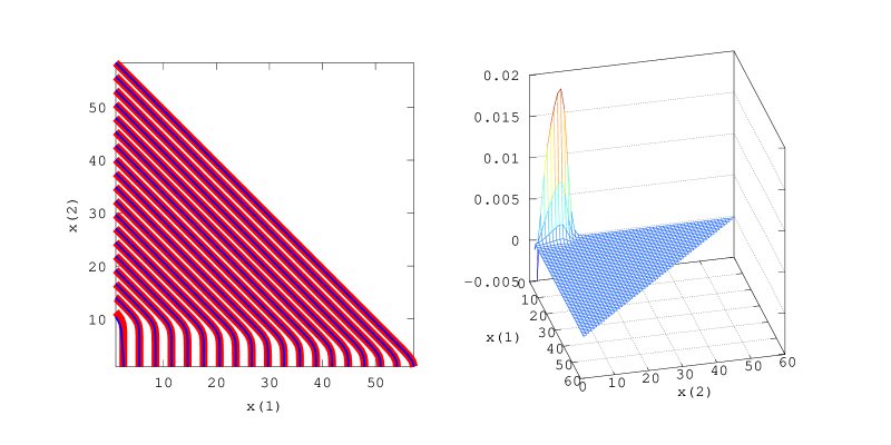
Figure 10:    On the left: level curves of $V_{n}$ (thin blue) and $W_{n}$ (thick red); on the right: the graph of $(W_{n}-V_{n})/W_{n}$

The first graph in Figure 10 are the level curves of $W_{n}$ of $V_{n}$; they all completely overlap except for the first one along the $x(2)$ axis. The second graph shows the relative error $(W_{n}-V_{n})/V_{n}$; we see that it appears to be zero except for a narrow layer around $0$ where it is bounded by $0.02$.

For $x=(1,0)$, the exact value for the probability $P_{x}(\tau_{60}<\tau_{0})$ is $1.1285\cdot 10^{-35}$ and the approximate value given by (164) equals $1.2037\cdot 10^{-35}$. Slightly away from the origin these quantities quickly converge to each other. For example, $P_{x}(\tau_{60}<\tau_{0})=4.8364\cdot 10^{-35}$, $f(x)=4.8148\cdot 10^{-35}$ for $x=(2,0)$ and $P_{x}(\tau_{60}<\tau_{0})=7.8888\cdot 10^{-31}$, $f(x)=7.8885\cdot 10^{-31}$ for $x=(9,0).$

For $x\in{\mathbb{Z}}_{+}^{2}$ and $g:{\mathbb{Z}}_{+}^{2}\rightarrow{\mathbb{R}}$ let ${\mathcal{D}}g$ denote the discrete gradient of $g$:

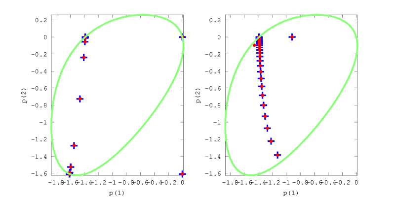
Figure 11:    ${\mathcal{D}}V_{n}(x)$ and ${\mathcal{D}}W_{n}(x)$ , $x=(5,\cdot)$; on the right the same functions for $x=(\cdot,1)$

$$({\mathcal{D}}g)(x)=(g(x+(1,0))-g(x),g(x+(0,1)-g(x)).$$

The large deviations analysis of $V_{n}$ suggests that $n{\mathcal{D}}V_{n}$ approximately equals $(\rho_{1},0)$ in a region around the $x(1)$ axis and $(\rho_{2},\rho_{2})$ elsewhere. These discrete gradients play a key role in the importance sampling estimation of the probability $P_{x}(\tau_{n}<\tau_{0})$. Since [14], it has been of interest to the author to understand how $n{\mathcal{D}}V_{n}(x)$ transitions from $(\rho_{1},0)$ to $(\rho_{2},\rho_{2})$ as $x$ moves from the $x(1)$-axis to the interior of $A_{n}$. The approximation of $V_{n}$ by $f$ also explains how this transition takes place. As an example let us graph the values of these gradients over the line $x(1)=5$ (any $x(1)$ value slightly away from $0$ will give similar results). The left panel of Figure 11 shows the discrete gradients ${\mathcal{D}}V_{n}$ and ${\mathcal{D}}W_{n}$ along this line; they overlap. The right panel of the same figure shows the same gradients over the line $x(2)=1$.

8.2 General two dimensional walk

Now let us consider the two dimensional network with the transition matrix

$$p=\left(\begin{matrix}0&0.15&0.1\\ 0.2&0&0.1\\ 0.24&0.06&0\end{matrix}\right).$$ (166)

For this example, we will need to use both $T_{n}^{i}$, $i=1,2$, to get good approximations of $P_{x}(\tau_{n}<\tau_{0})$ across all of $A_{n}.$ These two transformations will give us two limit unstable processes $Y^{1}$ and $Y^{2}$. The first will give good approximations along $\partial_{2}$ and the second along $\partial_{1}$. To combine their results into a single function, we will take their maximum.

The limit processes $Y^{1}$ and $Y^{2}$ have the following dynamics:

$$Y^{i}_{k+1}=Y^{i}_{k}+\pi_{i}(Y^{i}_{k},J^{i}_{k}),~{}~{}i=1,2,$$

where $J^{i}=J$ of (21) with $i=1,2$.

Remark 6.

$T_{n}^{2}$ equals $T_{n}^{1}$ after we exchange the node labels (i.e., node $1$ becomes $2$ and $2$ becomes $1$) This allows one to use the same computer code to compute either of the approximations by reordering the elements of the matrix $p$.

We want to compute

$$P_{y}(\tau^{1}<\infty),P_{y}(\tau^{2}<\infty),$$

where $\tau^{i}\doteq\inf\{k:Y^{i}_{k}\in\partial B\}$. We no longer have explicit finite formulas for these as we did in the tandem case. We will instead use a linear combination (a superposition) of basis functions of subsection 4.7 to approximate the function mapping $\partial B$ to $1$; the same linear combination of the Balayage of the basis functions (for which we have explicit formulas) will provide an approximation for the probabilities we seek. One way to do this is as follows (we give the details for $P_{y}(\tau^{1}<\infty)$, the procedure is identical for $P_{y}(\tau^{2}<\infty)$ ). As a first order approximation we use

$${\boldsymbol{A}}_{0}\doteq\frac{1}{C(r,{\boldsymbol{\alpha}}(r,1))}h_{r}=[(r,1),\cdot]-\frac{C(r,1)}{C(r,{\boldsymbol{\alpha}}(r,1))}[(r,{\boldsymbol{\alpha}}(r,1)),\cdot].$$

By Proposition 5.1, ${\boldsymbol{A}}_{0}$ is a harmonic function of $Y^{1}$.

For the $p$ of (166), $\beta_{1}(1)=r=0.42373$ and ${\boldsymbol{\alpha}}(r,1)=0.48123$. Then, by Proposition 4.10, ${\boldsymbol{A}}_{0}$ is $\partial B$ determined. These imply

$$|P_{y}(\tau^{1}<\infty)-{\boldsymbol{A}}_{0}|\leq P_{y}(\tau^{1}<\infty)\max_{y\in\partial B}|{\boldsymbol{A}}_{0}(y)-1|.$$ (167)

Set

$$c_{7}\doteq-\frac{C(r,1)}{C(r,{\boldsymbol{\alpha}}(r,1))}.$$

${\boldsymbol{A}}_{0}-1=c_{7}[(r,{\boldsymbol{\alpha}}(r,1)),\cdot]$ is geometrically decreasing on $\partial B$ and therefore it takes its greatest value at $n=0$ where it equals, for the present example, $3.8418<4$. This and (167) imply

$$\frac{1}{5}{\boldsymbol{A}}_{0}<P_{y}(\tau^{1}<\infty)<{\boldsymbol{A}}_{0}.$$

Thus, even with a single $Y$-harmonic pair of $\log$-linear functions, we are able to approximate $P_{y}(\tau^{1}<\infty)$ up to a constant term. To improve, approximate

$$c_{7}[r,{\boldsymbol{\alpha}}(r,1)),\cdot]$$

by a superposition of harmonic pairs of subsection 4.7 as follows. Consider the vector $\boldsymbol{b}\doteq c_{7}([(r,{\boldsymbol{\alpha}}(r,1)),({\mathrm{y}},{\mathrm{y}})],{\mathrm{y}}\in\{0,1,2,...,K\})\in{\mathbb{C}}^{K+1}$. If one thinks of the restriction of $c_{7}[(r,{\boldsymbol{\alpha}}(r,1)),\cdot]$ to $\partial B$ as a sequence, one truncates it to its first $K+1$ components to get $\boldsymbol{b}$; for $K$ large (for the present example we take $K=11$), the remaining tail of $c_{7}[(r,{\boldsymbol{\alpha}}(r,1)),\cdot]|_{\partial B}$ (its components from the $K+2^{nd}$ on) will be almost $0$. What we want to do is to construct basis vectors ${\boldsymbol{v}}_{i},i=0,1,2,...,K$, for ${\mathbb{C}}^{K+1}$ by truncating in the same way the restrictions to $\partial B$ of $K+1$ log-linear $Y$-harmonic functions and write $\boldsymbol{b}$ as a linear combination of the members of this basis. To construct our first basis element take the harmonic function $[(\beta(r_{1}),r_{1}),\cdot]$ of Proposition 4.8 and define ${\boldsymbol{v}}_{0}\doteq([(\beta(r_{1}),r_{1}),({\mathrm{y}},{\mathrm{y}})],{\mathrm{y}}\in\{0,1,2,...,K\})$. This gives us a vector in ${\mathbb{C}}^{K+1}$; to complete it to a basis for ${\mathbb{C}}^{K+1}$ we need $K$ more vectors. Set $\alpha_{j}\doteq Re^{ik\frac{2\pi j}{n+1}}$, where $R\in(r_{1},1)$ is to be specified and consider the $Y$-harmonic functions $h_{\beta_{1}(\alpha_{j})}$ of Proposition 5.1. We would like all of these to be $\partial B$-determined, for which

$$|\beta_{1}(\alpha_{j})|,|\alpha_{j}|,|{\boldsymbol{\alpha}}(\beta_{1}(\alpha_{j}),\alpha_{j})|<1$$ (168)

suffice; the second of these is satisfied by definition. The sufficient conditions we have derived for the rest, listed as Proposition 4.13, don’t cover the parameter values of the present example ((56) and $p(0,2)=0$ fail). Then, what we will do is to compute them explicitly (using (82) for ${\boldsymbol{\alpha}}(\beta_{1}(\alpha_{j}),\alpha_{j})$ and (53) for $\beta_{1}(\alpha_{j})$) and verify directly that (168) holds. Figure 12 shows the results of these calculations for $R=0.7$ and $K=11$ and indeed we see that $|\beta_{1}(\alpha_{j})|,|{\boldsymbol{\alpha}}(\beta_{1}(\alpha_{j}),\alpha_{j})|<1$ holds for all $j$.

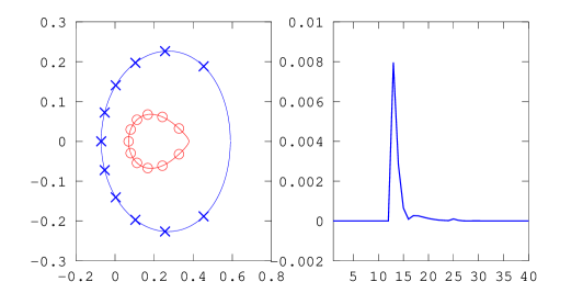
Figure 12:     $\beta_{1}(\alpha_{j})$’s (shown with x’s) and ${\boldsymbol{\alpha}}(\beta_{1}(\alpha_{j}),\alpha_{j})$’s (shown with ’o’s) on the ${\mathbb{C}}$-plane; the graph of the error $\Delta$ defined in (169)

Thus, by Proposition 4.10 all $h_{\beta_{1}(\alpha_{j})}$ are $\partial B$-determined. Define

$${\boldsymbol{v}}_{j}\doteq(h_{\beta_{1}(\alpha_{j})}({\mathrm{y}},{\mathrm{y}}),{\mathrm{y}}=0,1,2,...,K)\in{\mathbb{C}}^{K+1}.$$

Define the change of basis matrix ${\boldsymbol{B}}$ to consist of rows ${\boldsymbol{v}}_{0}$, ${\boldsymbol{v}}_{1}$,…,${\boldsymbol{v}}_{K}$; directly evaluating its determinant shows that ${\boldsymbol{B}}$ is invertable (this determinant is a polynomial in $\alpha_{j}$ and $\beta_{j}$, this can be used to show that, perhaps after perturbing $\alpha_{j}$, we can always assume ${\boldsymbol{B}}$ invertable). Define the coefficient vector

$$\psi\doteq{\boldsymbol{b}}{\boldsymbol{B}}^{-1}.$$

By definition,

$${\boldsymbol{A}}_{1}\doteq\psi(0)[(\beta(r_{1}),r_{1}),\cdot]+\sum_{j=1}^{K}\psi(j)h_{\beta_{1}({\alpha_{j}})}$$

equals $c_{7}[(r,{\boldsymbol{\alpha}}(r,1)),\cdot]$ over the set $\{({\mathrm{y}},{\mathrm{y}}),{\mathrm{y}}=0,1,2,...,K\}\subset\partial B$. That $|{\boldsymbol{\alpha}}(r,1)|<1$, (168) and $0<r_{1}<1$ imply that

$$\Delta({\mathrm{y}})\doteq|{\boldsymbol{A}}_{1}({\mathrm{y}},{\mathrm{y}})-c_{7}[(r,{\boldsymbol{\alpha}}(r,1)),({\mathrm{y}},{\mathrm{y}})]|\rightarrow 0$$ (169)

exponentially as ${\mathrm{y}}\rightarrow\infty$. Then one can explicitly find a bounded interval $[K+2,K^{\prime}]$ in which $\Delta({\mathrm{y}})$, $y\in{\mathbb{Z}}_{+}$, takes its maximum value. For $K=11$ and for the parameter values of the current example, this difference takes its maximum value at ${\mathrm{y}}=12$ (see the right panel of Figure 12) where it equals $0.00796<0.008$. These imply

$$0.992({\boldsymbol{A}}_{0}+{\boldsymbol{A}}_{1})<P_{y}(\tau^{1}<\infty)<1.008({\boldsymbol{A}}_{0}+{\boldsymbol{A}}_{1}),y\in B.$$

Set $g_{1}={\boldsymbol{A}}_{0}+{\boldsymbol{A}}_{1}$. Using exactly the same ideas we construct a function $g_{2}(y)$ approximating $P_{y}(\tau^{2}<\infty)$. $g_{1}$ and $g_{2}$ give two possible approximate values for $P_{x}(\tau_{n}<\tau_{0})$: $g_{1}(T^{1}_{n}(x))$ and $g_{2}(T^{2}_{n}(x))$; as pointed out in subsection 7.1 one expects

$$f(x)=\max(g_{1}(T^{1}_{n}(x)),g_{2}(T^{2}_{n}(x)))$$

to be the best approximation for $P_{x}(\tau_{n}<\tau_{0})$ that one can construct using $g_{1}$ and $g_{2}$. As in the previous section, we compare $f$ and $P_{x}(\tau_{n}<\tau_{0})$ in the logarithmic scale. Define $W_{n}(x)=-\frac{1}{n}\log f(x)$ ($V_{n}(x)$ is, as before, $V_{n}(x)=-\frac{1}{n}\log P_{x}(\tau_{n}<\tau_{0})$). Figure 13 shows the graph of $(V_{n}-W_{n})/V_{n}$ for the present case:

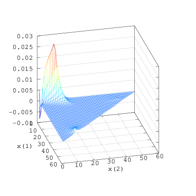
Figure 13:    Relative error for the nontandem two dimensional example

qualitatively it looks similar to the right panel of Figure 10; the relative error is near zero across $A_{n}$, except for a short boundary layer along the $x(2)$-axis; where it is bounded by $0.03$. One difference is the slight perturbation from $0$ of the relative error on $\partial A_{n}$ which comes from the approximation error depicted in the right panel of Figure 12.

The level curves of $V_{n}$, $-\frac{1}{n}\log g_{1}(T^{1}_{n}(x))$ are shown on the left panel of Figure 14; those of $V_{n}$ and $-\frac{1}{n}\log g_{2}(T^{2}_{n}(x))$ are given on the right panel. It is clear from these graphs that, indeed, as discussed above, $g_{i}(T^{i}_{n}(x))$ approximates $V_{n}$ well away from $\partial_{i}$.

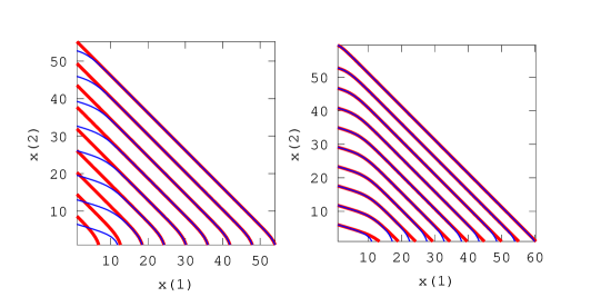
Figure 14:    Two approximations given by two limit processes

Finally, suppose we are given a function $h$ on $\partial A_{n}$. The algorithm above can also be used to approximate ${\mathbb{E}}_{y^{i}}\left[h(T^{i}_{n}(Y^{i}_{\tau^{i}}))1_{\{\tau^{i}<\infty\}}\right]$, $i=1,2$, and hence ${\mathbb{E}}_{x}\left[h(X_{\tau_{n}})1_{\{\tau_{n}<\tau_{0}\}}\right]$. We leave the analysis of this approximation to future work.

8.3 Tandem walk in higher dimensions

Take a four dimensional tandem system with rates, for example,

$$\lambda=1/18,\mu_{1}=3/18,\mu_{2}=7/18,\mu_{3}=2/18,\mu_{4}=5/18.$$

Let $f(y)$ denote the right side of (141). As before, define $V_{n}=-\log(P_{x}(\tau_{n}<\tau_{0}))/n$ and $W_{n}=-\log f(T_{n}(x))/n$. The level curves of $V_{n}$ and $W_{n}$ and the graph of the relative error $(V-W)/V$ for $x=(0,0,i,j)$, $i,j\leq n$, are shown in Figure 15; once again, qualitatively, these graphs show results similar to those observed for the earlier examples: almost zero relative error across the domain selected, except for a boundary layer along the $x(4)$-axis, where the relative error is bounded by $0.05.$

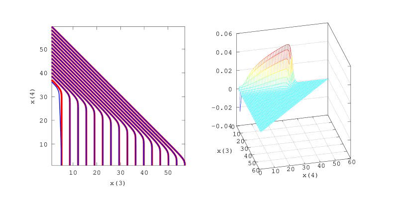
Figure 15:    Level curves and relative error in four dimensions

As our last example, consider the $14$-tandem queues with parameter values shown in Figure 16.

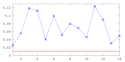
Figure 16:    The service rates (blue) and the arrival rate (red) for a $14$-dimensional tandem Jackson network

For $n=60$, $A_{n}$ contains $60^{14}/14!=8.99\times 10^{13}$ states which makes impractical an exact calculation via iterating (35). On the other hand, (141) has $2^{14}-1=16383$ summands and can be quickly calculated. Define $W_{n}$ as before. Its graph over $\{x:x(4)+x(14)=60,x(j)=0,j\neq 4,14\}$ is depicted in Figure 17.

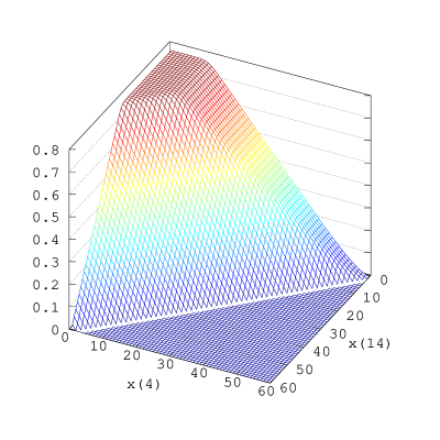
Figure 17:    The graph of $W_{n}$ over $\{x:x(4)+x(14)=60,x(j)=0,j\neq 4,14\}$

For a finer approximation of $P_{(1,0,\cdots,0)}(\tau_{n}<\tau_{0})$ we use importance sampling based on $W_{n}$. With $12000$ samples, IS gives the estimate $7.53\times 10^{-20}$ with an estimated $95\%$ confidence interval $[6.57,8.48]\times 10^{-20}$ (rounded to two significant figures). The value given by our approximation (141) for the same probability is $f((1,0,\cdots,0))=1.77\times 10^{-20}$ which is approximately $1/4^{th}$ of the estimate given by IS. The LD estimate of the same probability is $(\lambda/\min_{i=1}^{14}(\mu_{i}))^{60}=4.15\times 10^{-23}$. The discrepancy between IS and (141) quickly disappears as $x(1)$ increases. For example, for $x(1)=4$, IS gives $2.47\times 10^{-19}$ and (141) gives $2.32\times 10^{-19}$.

9 Conclusion

The foregoing analysis points to a number of future directions for research. We state some of them here.

9.1 Constrained diffusions with drift and elliptic equations with Neumann boundary conditions

Diffusion processes are weak limits of random walks. Thus, the results of the previous sections can be used to compute/approximate Balayage and exit probabilities of constrained unstable diffusions. We give an example demonstrating this possibility.

For $a,b>0$ let $X$ be the the constrained diffusion on ${\mathbb{R}}\times{\mathbb{R}}_{+}$ with infinitesimal generator $L$ defined as

$$f\rightarrow Lf,Lf=\langle\nabla f,((2a+b),(a-b))\rangle+\frac{1}{6}\nabla^{2}f\cdot\left(\begin{matrix}2&1\\ 1&2\end{matrix}\right),$$

where $\nabla^{2}$ denotes the Hessian operator, mapping $f$ to its matrix of second order partial derivatives. On $\{x:x(2)=0\}$ $X$ is pushed up to remain in ${\mathbb{R}}\times{\mathbb{R}}_{+}$ (the precise definition involves the Skorokhod map, see, e.g., [11]). $a,b>0$ implies that, starting from $B=\{x:x(1)>x(2)\}$, $X$ has positive probability of never hitting $\partial B=\{x:x(1)=x(2)\}.$ Let $\tau$ be the first time $X$ hits $\{x:x(1)=x(2)\}$. Proposition 6.5 for $d=2$ suggests

$$P_{x}(\tau<\infty) =e^{-(a+2b)3(x(1)-x(2))}+\frac{a+2b}{a-b}e^{-(a+2b)3(x(1)-x(2))}e^{-(2a+b)3x(2)}$$

$$~{}~{}-\frac{a+2b}{a-b}e^{-3(2a+b)x(1)},x\in B.$$ (170)

One can check directly that the right side of the last display satisfies

$$LV=0,~{}~{}\langle\nabla V,(0,1)\rangle=0,x\in\partial_{2}.$$

This and a verification argument similar to the proof of Proposition 4.10 will imply (9.1). Almost the same argument for general $d$ gives an explicit formula for the solution of the $d$ dimensional version of the above elliptic equation on ${\mathbb{R}}\times{\mathbb{R}}_{+}^{d}$, with $2^{d-1}-1$ Neumann boundary conditions on $\partial({\mathbb{R}}\times{\mathbb{R}}_{+}^{d}).$

9.2 Solutions to perturbed nonlinear PDE

As indicated in the introduction, classical large deviations analysis leads (at least for Markov processes) to a deterministic first order HJB equation. To improve the approximation provided by the solution of this first order PDE, one can add nonlinear second order perturbation terms to it [17]. We expect the ideas of the paper to bear on the task of computing approximate solutions of the perturbed second order nonlinear PDE related to the probabilities treated in the present paper.

9.3 Extension to other processes and domains

In the foregoing sections, we have computed approximations to the Balayage operator and exit probabilities of a class of constrained random walks in two stages: 1) use an affine change of coordinates to move the origin to a point on the exit boundary and take limits; as a result, some of the constraints in the prelimit process disappear and one obtains as a limit process an unstable constrained random walk; 2) find a class of basis functions on the exit boundary on which the Balayage operator of the limit process has a simple action; then try to approximate any other function on the exit boundary with linear combinations of the functions in the basis class. The type of problem we have studied here is of the following form: there is a process $X$ with a certain law of large number limit which takes $X$ away from a boundary $\partial A_{n}$ towards a stable point or a region; $\tau_{0}$ is the first time the process gets into this stable region. We are interested in the probability $P(\tau_{n}<\tau_{0})$ and the associated Balayage operator. We expect the first step to be applicable to a range of problems that fit into this scenario. The second stage obviously depends on the particular dynamics of the original process and the geometry of the exit boundary. It remains to be explored for which processes and boundaries it is possible to construct classes of simple basis functions. Even very simple changes in the dynamics or in the boundary geometry from those covered in this paper may lead to different types of basis functions. We hope to treat the tandem walk case with a separate boundary in an upcoming work.

9.4 Harmonic functions with polynomial terms

Let us confine ourselves, for the purposes of this brief comment, to tandem queues. If $\mu_{1}=\mu_{2}$, (91) no longer holds and indeed (163) is not well defined (because of the $\mu_{1}-\mu_{2}$ in the denominator of the first ratio). One way to remedy this is to replace the right side of (163) by the limit of the same expression as $\mu_{1}\rightarrow\mu_{2}$, which gives

$$P_{y}(\tau<\infty)=\rho^{y(1)}+\frac{\mu-\lambda}{\mu}(y(1)-y(2))\rho^{y(1)-y(2)},$$ (171)

where $\mu_{1}=\mu_{2}=\mu$ and $\rho=\lambda/\mu.$ Similarly, in three dimensions one gets, for example, for $\mu_{1}=\mu_{2}=\mu_{3}$

$$P_{y}(\tau<\infty)=\rho^{\bar{y}(1)}\left(\frac{1}{2}c_{0}^{2}(\bar{y}(1))^{2}\rho^{y(2)+y(3)}+\rho^{y(3)}\left(\left(\frac{c_{0}^{2}}{2}+y(3)c_{0}^{2}\right)\rho^{y(2)}+c_{0}\right)\bar{y}(1)+1\right),$$

where $c_{0}=(\mu-\lambda)/\mu$ and $\bar{y}(1)=y(1)-(y(2)+y(3))$. Similar limits can be computed explicitly for the cases $\mu_{1}=\mu_{2}\neq\mu_{3}$, $\mu_{1}=\mu_{3}\neq\mu_{2}$ and $\mu_{1}\neq\mu_{2}=\mu_{3}$. Generalization of these results to higher dimensions and more general topologies remain for future work.

9.5 The boundary layers of $V_{n}$ and subsolution based importance sampling algorithms

The works [14, 5] develop IS algorithms based on subsolutions of (148) to estimate $p_{n}$. These works and others which followed them express most of their functions in a law of large numbers scale (as we do in Sections 3 and 7). We will express everything in unscaled coordinates in the discussion below. Again, to be brief, we will limit ourselves to formal comments on two tandem queues. Details and generalizations remain for future work.

For certain values of system parameters, $V_{n}$ of (165) may manifest a boundary layer, where its discrete gradient sees a rapid change near the boundaries of its state space. This happens when $\mu_{1}=\mu_{2}$ for the case of two tandem queues with a boundary layer along the $x(1)$ axis. Here is one interpretation of the subsolution approach of [5, 14] in the present context (i.e., two tandem queues and $\mu_{1}=\mu_{2}$): the discrete gradient of the large deviation value function

$$\bar{V}_{n}(x)\doteq-\frac{1}{n}\log\left(\rho^{n-(x(1)+x(2))}\right)$$

approximates the discrete gradient of $V_{n}$ well everywhere except along a boundary layer along the $x(1)$ axis; the subsolutions constructed in [5, 14] are perturbations of $\bar{V}_{n}$ which attempt to approximate the discrete gradient of $V_{n}$ also in this boundary layer. The subsolutions constructed in these works involve a parameter $\epsilon_{n}$ that satisfy

$$n\epsilon_{n}\rightarrow\infty,~{}~{}\epsilon_{n}\rightarrow 0$$ (172)

and have boundary layers of constant width parallel to the $x(1)$ axis; $\epsilon_{n}$ determines the width of the boundary layer. Although [5, Theorem 3.8] says that (172) suffices for the IS algorithm defined by the subsolutions to be asymptotically optimal, [14, subsection 2.3.3] observes that a good performance of the algorithm for finite $n$ (accurate estimation results with bounded estimated relative error) requires a finer specification of $\epsilon_{n}$ and hence of the size of the approximating boundary layer. How to measure the size of the boundary layer of $V_{n}$ (and use this information to specify $\epsilon_{n}$) more precisely has remained an open problem since the inception of the subsolution approach. With (171) we now see that the correct way to add a boundary layer to $\bar{V}_{n}$ (so that it has a boundary layer mimicking that of $V_{n}$) is to perturb it to

$$W_{n}(x)=-\frac{1}{n}\log\left(\rho^{n-(x(1)+x(2))}+\frac{\mu-\lambda}{\mu}(n-(x(1)+x(2)))\rho^{n-x(1)}\right).$$ (173)

Proposition 7.1 and the numerical example of subsection 8.1 suggest that the boundary layer of $W_{n}$ matches that of $V_{n}$ as $n$ increases.

The definitions (149) and (150) give an alternative construction of smooth subsolutions with explicit boundary layers (the region where $\nabla V_{i}^{c,\epsilon}={\boldsymbol{r}}_{1}$). In contrast, the boundary layer of $W_{n}$ is expressed implicitly in its definition (173). Let us now try to quantify explicitly the size and the shape of the boundary layer of $W_{n}$ and thus that of $V_{n}$.

Define

$$\hat{W}(y)\doteq-\log\left(\rho^{y(1)-y(2)}+\frac{\mu-\lambda}{\mu}(y(1)-y(2))\rho^{y(1)}\right).$$

Then $W_{n}(x)=\frac{1}{n}\hat{W}(T_{n}(x)).$ It suffices to calculate the boundary layer of $\hat{W}$; this we can transform by $T_{n}$ to get that of $W_{n}$. We will specify the boundary layer by its boundary ${\boldsymbol{l}}:{\mathbb{R}}_{+}\rightarrow{\mathbb{R}}_{+}$; the layer will be defined as $\{y:y(2)\leq{\boldsymbol{l}}(y(1))\}.$ The defining property of the layer is that it is the region where the gradient of $\hat{W}$ rapidly changes. Away from the boundary $\{y(2)=0\}$ $\hat{W}$ behaves like the linear function $(y(1)-y(2))\log(\rho)$ whose directional derivative $\nabla_{(1,1)}\hat{W}$ in the direction $(1,1)$ is zero. And indeed the same is true for $\hat{W}$ itself on $\{y:y(1)=y(2)\}$, i.e.,

$$\nabla_{(1,1)}(\hat{W})\doteq\frac{\partial\hat{W}}{\partial y(1)}(y)+\frac{\partial\hat{W}}{\partial y(2)}(y)=0,y\in\{y:y(1)=y(2)\}.$$

Furthermore, for fixed $y(1)$, $\nabla_{(1,1)}\hat{W}(y)$ is decreasing in $y(2)$ and the above display implies that this directional derivative hits zero on $\partial_{1}$. We will define ${\boldsymbol{l}}(y(1))$ as the point where the value of $\nabla_{(1,1)}\hat{W}$ is half of its value at $(y(1),0)$, i.e.,

$${\boldsymbol{l}}(y(1))\doteq y(2)^{*}$$ (174)

where $y(2)^{*}$ is the unique solution of

$$(y(1)-y(2)^{*})\left(1+\frac{1}{2}\frac{\mu-\lambda}{\mu}y(1)\right)=\frac{1}{2}y(1)\rho^{-y(2)^{*}}.$$

$\boldsymbol{l}$ is increasing $y(1)$: this implies that when transformed by $T_{n}$ it defines a boundary layer for $W_{n}$ (and hence for $V_{n}$) that narrows down as it extends toward the point $(n,0)$. In contrast, the subsolutions developed in [5, 14] have boundary layers of constant size, i.e., parallel to the $x(1)$ axis. The graph of $x(1)\rightarrow{\boldsymbol{l}}((n-x(1)))$, $x(1)\in[0,n]$, and the level sets of $V_{n}$ for $n=40$, $\lambda=0.2,$ and $\mu=0.4$ are shown in Figure 18.

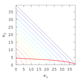
Figure 18:    The contours of $V_{n}$ for $n=40$, $\lambda=0.2$ , $\mu=0.4$ and its boundary layer computed using $\boldsymbol{l}$ of (174)

References

- [1] Søren Asmussen and Peter Glynn, Stochastic simulation: Algorithms and analysis, vol. 57, Springer Science & Business Media, 2007.
- [2] Hong Chen and David Yao, Fundamentals of queueing networks: Performance, asymptotics, and optimization, vol. 46, Springer Science & Business Media, 2013.
- [3] Amir Dembo and Ofer Zeitouni, Large deviations techniques and applications, second ed., Applications of Mathematics (New York), vol. 38, Springer-Verlag, New York, 1998. MR MR1619036 (99d:60030)
- [4] Paul Dupuis and Richard Ellis, A weak convergence approach to the theory of large deviations, John Wiley & Sons, New York, 1997.
- [5] Paul Dupuis, Ali Devin Sezer, and Hui Wang, Dynamic importance sampling for queueing networks, Annals of Applied Probability 17 (2007), no. 4, 1306–1346.
- [6] Richard Durrett, Probability: theory and examples, second ed., Duxbury Press, Belmont, CA, 1996. MR MR1609153 (98m:60001)
- [7] John Eaton, Gnu octave manual, Network Theory Limited, 2002.
- [8] Paul Glasserman and Shing-Gang Kou, Analysis of an importance sampling estimator for tandem queues, ACM Transactions on Modeling and Computer Simulation 5 (1995), 22–42.
- [9] Phillip Griffiths, Introduction to algebraic curves, American Mathematical Society, 1989.
- [10] Frank Kelly, Reversibility and stochastic networks, Cambridge University Press, 2011.
- [11] Harold Kushner and Paul Dupuis, Numerical methods for stochastic control problems in continuous time, vol. 24, Springer Science & Business Media, 2001.
- [12] Daniel Revuz, Markov chains, North-Holland, 1984.
- [13] Philippe Robert, Stochastic networks and queues, stochastic modelling and applied probability series, vol. 52, Springer, New York, 2003.
- [14] Ali Devin Sezer, Dynamic importance sampling for queueing networks, ph.d. thesis, Brown University Division of Applied Mathematics, 2005.
- [15] Adam Shwartz and Alan Weiss, Large deviations for performance analysis, Stochastic Modeling Series, Chapman & Hall, London, 1995, Queues, communications, and computing, With an appendix by Robert J. Vanderbei. MR MR1335456 (96i:60029)
- [16] David Siegmund, Importance sampling in the Monte Carlo study of sequential tests, The Annals of Statistics 4 (1976), 673–684.
- [17] Sathamangalam Ranga Iyengar Srinivasa Varadhan, Large deviations and applications, CBMS-NSF Regional Conference Series in Applied Mathematics, vol. 46, Society for Industrial and Applied Mathematics (SIAM), Philadelphia, PA, 1984. MR MR758258 (86h:60067b)