Separated matter and antimatter domains
with vanishing domain walls

Abstract

We present a model of spontaneous (or dynamical) $C$ and $CP$ violation where it is possible to generate domains of matter and antimatter separated by cosmologically large distances. Such $C$($CP$) violation existed only in the early universe and later it disappeared with the only trace of generated baryonic and/or antibaryonic domains. So the problem of domain walls in this model does not exist. These features are achieved through a postulated form of interaction between inflaton and a new scalar field, realizing short time $C$($CP$) violation.

I Introduction

Our local cosmological neighborhood is made of baryons, while fraction of antimatter, presumably of astrophysical origin, is vanishingly small. So the observations indicate that the universe is 100% baryo-asymmetric, at least locally. The Baryon Asymmetry (of the Universe), BAU, cannot be explained in the frameworks of the Standard Model (SM) of particle physics. Alongside with evidence for dark matter and dark energy it is considered as unambiguous proof of the existence of new physics beyond SM.

Many quite different extensions of the SM and various scenarios for the BAU generation were suggested in the literature, for a review see e.g. Refs. BAU_1 ; BAU_2 ; BAU_3 ; BAU_4 ; BAU_5 . Typically, consideration is restricted to the models where the universe is asymmetric globally. This is the simplest possibility. However, it is not excluded that the real universe may be globally symmetric. It may consist of domains of matter and antimatter, and if the domains are sufficiently large and far away, they may escape observational constraints on matter-antimatter annihilation at the domain boundaries. In the simplest version of the scenario the distance to the nearest domain of antimatter should be close to the present day cosmological horizon annihilation_constr .

Corresponding particle physics models, leading to the universe creation with abundant antimatter domains were suggested and developed in the past. While being more involved, the models of this type also suffer from the inherent problem – a domain wall problem DWProblem . Indeed, BAU can be generated only if $CP$ violation is sufficiently strong, beyond the SM capabilities. In addition, in globally symmetric universe $CP$ should have different signs in different domains. This non-trivial pattern of $CP$ violation could be provided by a dedicated physical field, one way or another. Therefore, unavoidably, domains with different $CP$ phase would be separated by domain walls with unacceptably high energy density, in conflict with observations. There is only one way out of this restriction. Namely, domains with different sign (and possibly strength) of $CP$ violation should exist only in the universe past and should disappear by now, all together with domain walls, though their effects in the form of matter and antimatter objects would survive to the present day.

One class of models where this can be achieved has been suggested in Refs. Kuzmin_1 ; Kuzmin_2 ; Kuzmin_3 ; Kuzmin_4 . The main idea behind is a possibility of an unusual symmetry behavior at high temperatures. It is well known that a symmetry, which is broken in vacuum, at high temperatures tends to be restored. But in general, the situation is not that simple and straightforward. It is also possible that a symmetry is broken only in a particular range of temperatures, i.e. it is restored at the highest as well as at the lowest temperatures, for the particular models and details see Kuzmin_1 ; Kuzmin_2 ; Kuzmin_3 ; Kuzmin_4 . This is just what is needed for a matter-antimatter domain generation without domain wall problem. However, if a model is based on the unusual symmetry behavior at high temperatures, then the size of domains will be too small from the cosmological point of view. Such models are still interesting, because they could provide a local excess of antimatter, which would be large compared to the capabilities of astrophysical sources, if an excess AntiExcess turns out to be real. But cosmologically large and separated domains of antimatter cannot be created by this mechanism. Cosmology with domains of matter and antimatter was discussed in the lectures fs ; ad , where a list of relevant references can be found. As argued in Ref. larsson , domain walls could be also eliminated if the vacua in the model were not exactly degenerate. In this case the higher energy vacuum would be ”swallowed” by the lower energy one if the energy difference is sufficiently high.

In the present paper we suggest another scenario of unusual symmetry behavior. Now this happens during inflationary stage in the universe evolution. Domains with different sign of $CP$ disappear by now also, so the domain wall problem is absent. However, they appeared during inflation and survived at the baryogenesis epoch, therefore, cosmologically large domains of matter and antimatter could be created.

II Model

In the suggested model the difference between matter and antimatter is generated by pseudoscalar field $\chi$ which interacts with inflaton field $\Phi$. We assume the following Lagrangian:

$$L=L_{\Phi}+L_{\chi}+L_{int},$$ (1)

where

$$L_{\Phi} = \frac{1}{2}(\partial\Phi)^{2}-\frac{1}{2}M^{2}\Phi^{2},$$ (2)

$$L_{\chi} = \frac{1}{2}(\partial\chi)^{2}-\frac{1}{2}m^{2}\chi^{2}-\frac{1}{4}\lambda_{\chi}\chi^{4},$$ (3)

$$L_{int} = \mu^{2}\chi^{2}V(\Phi).$$ (4)

Here the metric tensor enters into kinetic terms in the usual way, and $M,m,\lambda_{\chi},\mu$ are some constant parameters, with $M,m,\mu$ having dimension of mass, $\lambda_{\chi}$ being dimensionless. We do not include the quartic term $-\lambda_{\Phi}\Phi^{4}/4$ in the Lagrangian, though it possibly may lead to some interesting consequences. This case will be studied elsewhere. The dimensionless function $V(\Phi)$ is chosen in the way that it is non-zero only when $\Phi$ is close to some constant value $\Phi_{0}$. In this paper we choose it as Gaussian function

$$V(\Phi)=\exp\left[-\frac{(\Phi-\Phi_{0})^{2}}{2\Phi_{1}^{2}}\right],$$ (5)

though other forms may be possible. The plot of function $V(\Phi)$ (see Fig. 1) is a bell-shaped curve. Parameters $\Phi_{0}$ and $\Phi_{1}$ have dimension of mass and indicate position of the ”bell” center and characteristic width of the ”bell”, respectively.

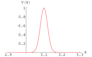
Figure 1: Function $V(\Phi)$. The parameters are $\Phi_{0}=3.1\,m_{Pl}$ and $\Phi_{1}=0.02\,m_{Pl}$. Field $\Phi$ is measured in units of $m_{Pl}$ and $V(\Phi)$ is dimensionless.

The equations of motion have the form:

$$\ddot{\Phi}+3H\dot{\Phi}+M^{2}\Phi+\mu^{2}\chi^{2}\frac{\Phi-\Phi_{0}}{\Phi_{1}^{2}}V(\Phi) = 0,$$ (6)

$$\ddot{\chi}+3H\dot{\chi}+m^{2}\chi+\lambda_{\chi}\chi^{3}-2\mu^{2}\chi V(\Phi) = 0,$$ (7)

where $H=\dot{a}/a$ is the Hubble parameter, $a(t)$ is the cosmological scale factor which enters into the FLRW metric as

$$ds^{2}=dt^{2}-a^{2}(t)\,d{\bf x}^{2}.$$ (8)

It is assumed here that fields $\Phi$ and $\chi$ depend only on time, $\Phi=\Phi(t)$ and $\chi=\chi(t)$.

The Hubble parameter is expressed through the energy density $\rho$ as

$$H=\sqrt{\frac{8\pi\rho}{3m_{Pl}^{2}}}=\sqrt{\frac{8\pi}{3m_{Pl}^{2}}\left(\frac{\dot{\Phi}^{2}}{2}+\frac{M^{2}\Phi^{2}}{2}+\frac{\dot{\chi}^{2}}{2}+\frac{m^{2}\chi^{2}}{2}+\frac{\lambda_{\chi}\chi^{4}}{4}-\mu^{2}\chi^{2}V(\Phi)\right)}\ ,$$ (9)

where $m_{Pl}\approx 1.2\cdot 10^{19}$ GeV is the Planck mass.

The interaction introduced above leads to the following scenario. During inflation the magnitude of the inflaton field $\Phi$ decreases and when it reaches vicinity of $\Phi_{0}$ two minima appear in the potential

$$U(\Phi,\chi)=\left(\frac{1}{2}m^{2}-\mu^{2}V(\Phi)\right)\chi^{2}+\frac{1}{4}\lambda_{\chi}\chi^{4}+\frac{1}{2}M^{2}\Phi^{2}$$ (10)

at constant $\Phi$, so the point $\chi=0$ becomes local maximum (see Fig. 2).

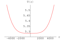
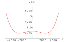
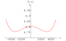
Figure 2: Potential $U(\Phi,\chi)$ at constant $\Phi$. The left plot corresponds to the moment when the effective mass of $\chi$ becomes zero, i.e. when $m^{2}/2-\mu^{2}V(\Phi)=0$, therefore $\Phi=\Phi_{0}+2\Phi_{1}\sqrt{\ln{(\sqrt{2}\mu/m)}}$. The middle and the right plots show the moments when $\Phi=\Phi_{0}+\Phi_{1}$ and $\Phi=\Phi_{0}$, respectively; the squared effective mass of $\chi$ is negative in these cases. The parameters are $\Phi_{0}=3.1\,m_{Pl}$, $\Phi_{1}=0.02\,m_{Pl}$, $\mu=10^{-4}m_{Pl}$ and $m=10^{-10}m_{Pl}$. Field $\chi$ is measured in units of $M$ and $U(\Phi,\chi)$ is measured in units of $10^{-12}\,m_{Pl}^{4}$.

Therefore, in the spatial regions where the field $\chi$ turns out to be positive (due to fluctuations) it rolls down to the positive minimum $\eta>0$, and in the regions where $\chi$ is negative it goes to the negative minimum $-\eta<0$. Thus one can substitute $\chi=\widetilde{\chi}+\eta$ and $\chi=\widetilde{\chi}-\eta$, respectively, where $\eta$ and $-\eta$ have the meaning of the vacuum expectation values $<\chi>$. The field $\tilde{\chi}$ includes quantum fluctuations around new vacua but in what follows we consider only a classical part of it $\tilde{\chi}=\tilde{\chi}(t)$.

Let us suppose that fermions enter into theory through the following Lagrangian:

$$L_{\psi}=\bar{\psi}(i\hat{\partial}-m_{\psi})\psi-g\chi\bar{\psi}i\gamma_{5}\psi,$$ (11)

where $g$ is dimensionless constant. This Lagrangian respects all discrete symmetries, as the field $\chi$ is $P$-odd and $C$-even. Substituting $\chi=\widetilde{\chi}\pm\eta$ and carrying out the axial rotation $\psi\rightarrow{\rm exp}(i\alpha\gamma_{5})\,\psi$ with $\alpha=1/2\,{\rm arctan}(\mp\eta g/m_{\psi})$ in order to eliminate the term $\bar{\psi}i\gamma_{5}\psi$, we find

$$L_{\psi}=\bar{\psi}(i\hat{\partial}-M_{\psi})\psi-g\frac{m_{\psi}}{M_{\psi}}\widetilde{\chi}\bar{\psi}i\gamma_{5}\psi\mp g^{2}\frac{\eta}{M_{\psi}}\widetilde{\chi}\bar{\psi}\psi,$$ (12)

where $M_{\psi}=\sqrt{m_{\psi}^{2}+g^{2}\eta^{2}}$. The last two terms in (12) behave in opposite ways under $CP$-conjugation, so this Lagrangian violates $CP$-symmetry. Moreover, the sign of the last term in (12) depends on the choice of the minimum (positive or negative) where the field $\chi$ has rolled down. Thus all the space turns out to be divided into domains with opposite signs of $CP$ violation DWProblem . These domains are separated by domain walls which should vanish at the present epoch, because the field $\chi$ ultimately tends to the final minimum at $\chi=0$ independently of its initial position at $\chi=\pm\,\eta$, as we see in what follows.

We expect that the distances between domains, as well as domain sizes exponentially grow with the scale factor $a(t)$, so at the present time these domains are of cosmological size and they are separated by large distance which prevents the annihilation at their boundaries. According to Ref. annihilation_constr , a very large piece of space between the domains, devoid of baryons, would lead to too large angular fluctuations of the CMB temperature. On the other hand, if the distance between domains is smaller than the baryon diffusion length, they would be able to meet successfully their counterparts and to annihilate. These arguments resulted in the conclusion that the nearest domains should be at the cosmologically large distance from us, about a few Gpc. On the other hand, the effects of the cosmological inhomogeneity, not yet studied, could inhibit the baryon diffusion and would relax the bound on the distance to the nearest antimatter domain.

However, $CP$ violation described by Lagrangian (12) is operative only when the field $\chi$ sits near the temporary minimum, $\pm\,\eta$, i.e. when the expression $\chi=\widetilde{\chi}\pm\eta$ is valid, where $\widetilde{\chi}$ are small quantum fluctuations. In our model this is true only during inflation. Consequently such $CP$ violation is not efficient for baryogenesis, because the generated at this period baryon asymmetry would be exponentially inflated away. Hence successful baryogenesis should take place after the end of inflation. Though the minima at $\chi=\pm\eta$ disappeared after inflation, still the classical field $\chi(t)$ remained non-vanishing for a long time after inflation was over. The classical field $\chi$ slowly tends to zero and if baryogenesis could proceed fast enough, while $\chi\neq 0$, the $CP$ violation induced by non-zero $\chi(t)$ might be effective. In these circumstances more efficient $CP$ violation would originate from the imaginary part of the quark effective mass matrix proportional to $\chi(t)$ and to this end at least 3 quark families are necessary KM . The only difference with the standard case is that the contribution to $CP$-odd phase of the mass matrix is not constant anymore, but slowly changes with time. In more detail this is described below at the end of section IV.

Now let us consider what happens at different stages of the scenario, so we will be able to put the limits on initial conditions and parameters of the model.

For simplicity we assume, though it is not necessary, that the impact of field $\chi$ on cosmological expansion at inflationary stage is negligible. To this end we suppose that the energy density of $\Phi$ dominates over that of $\chi$ and the energy density of their interaction. Since the field $\Phi$ is not affected by $\chi$, the evolution of $\Phi$ is described by standard inflation theory, which is taken here as the usual slow-roll regime of inflation. In this approximation the second derivative term and the interaction term proportional to $V(\Phi)$ in the inflaton equation of motion (6) can be neglected. Therefore, we find

$$\dot{\Phi}=-\frac{M^{2}\Phi}{3H}.$$ (13)

We suppose that the term $M^{2}\Phi^{2}/2$ makes the dominant contribution to the energy density $\rho$, so the Hubble parameter (9) is equal to $H=\sqrt{4\pi/3}\,(M/m_{Pl})\Phi$, and the equation (13) can be easily integrated giving

$$\Phi(t)=\Phi_{in}-\frac{Mm_{Pl}\,t}{2\sqrt{3\pi}},$$ (14)

where $\Phi_{in}$ is an initial value of $\Phi$. In this scenario of inflation the Hubble parameter gradually decreases, $H\sim\Phi$, and to obtain a sufficiently long inflation with duration

$$\int\limits_{0}^{t_{end}}H(t)dt\approx\frac{1}{2}H_{in}t_{end}=\frac{2\pi\Phi^{2}_{in}}{m^{2}_{Pl}}>70,$$ (15)

it is sufficient to take $\Phi_{in}\gtrsim 3.3\,m_{Pl}$. In Eq. (15) $H_{in}=\sqrt{4\pi/3}\,(M/m_{Pl})\Phi_{in}$ is the initial value of the Hubble parameter and $t_{end}=2\sqrt{3\pi}\,\Phi_{in}/(Mm_{Pl})$ is the time moment when $\Phi=0$, see (14). To be more precise, inflation ends when the Hubble parameter becomes approximately equal to the mass of the inflaton, $H_{fin}\sim M$, because at this moment the exponential expansion terminated and the inflaton field started to oscillate around zero with frequency $M$. Correspondingly the exponential expansion turned into the matter dominated one, $a\sim t^{2/3}$. So the final amplitude of $\Phi$ should be taken as $\Phi_{fin}=\sqrt{3/(4\pi)}\,m_{Pl}$. Correspondingly the final time would be slightly changed.

In order to avoid too large density perturbations one should choose the value of the inflaton mass $M$ in the range $10^{-7}\lesssim M/m_{Pl}\lesssim 10^{-6}$; accordingly we take $M=10^{-6}\,m_{Pl}$.

To arrange the desired scenario we should set the value of $\Phi_{0}$ still at inflationary stage such that the distances between different domains and the domain sizes exponentially expanded up to cosmologically large scales.

We can make a naive estimate of the necessary duration of inflation after the inflaton field reached value $\Phi=\Phi_{0}$. Suppose that at the present time the size of a domain is about 10 Mpc. If the characteristic scale of the initial energy/temperature is of the order of $T$, then it is natural to expect the domain size to be of the order of $l\sim 1/T$. Due to regular cosmological expansion it would increase to $z=(1/T)(T/3K)\sim 0.1$ cm. So during inflation the domains should be expanded by a factor of (10 Mpc)/(0.1 cm) $\sim 3\cdot 10^{26}$. Therefore, we require that after $\Phi$ passes $\Phi_{0}$ the inflation should last at least 60 e-foldings, $N_{e}={\rm ln}\,(3\cdot 10^{26})\simeq 60$,

$$\int\limits_{t_{0}}^{t_{end}}H(t)dt=\frac{2\pi\Phi_{0}^{2}}{m_{Pl}^{2}}\gtrsim N_{e}\simeq 60,$$ (16)

$$\frac{\Phi_{0}}{m_{Pl}}=\sqrt{\frac{N_{e}}{2\pi}}\approx 3.1,$$ (17)

where $t_{0}$ is the time when $\Phi=\Phi_{0}$. However, since the process initiated at inflationary stage, when temperature in classical sense did not exist, the characteristic scale of the seed of the domain should be of the order of the inverse Hubble parameter, $l\sim 1/H\sim 1/M$. So the obtained above result would be shifted to $N\approx 60+\ln(M/T_{heat})$, where $T_{heat}$ is the universe temperature after inflation. Since typically $T_{heat}\approx(10^{-5}\div 10^{-6})\,m_{Pl}$ the estimate presented above remains practically unchanged.

Depending upon the value of $\Phi$, there are three different regimes of the evolution of the field $\chi$:

1. Initial stage: $\Phi>\Phi_{0}$ and $\left(\Phi-\Phi_{0}\right)\gg\Phi_{1}$.

   The mass of $\chi$ is supposed to be small in comparison with the expansion rate, $m<H$, so field $\chi$ sits near the minimum of its potential at $\chi=0$ (see left plot in Fig. 2), with the dispersion of the order of $\langle\chi^{2}\rangle\sim{\rm min}\{H^{4}/m^{2},H^{2}/\sqrt{\lambda_{\chi}}\}$ (see e.g. Gorbunov ).

2. Second stage: $\left|\Phi-\Phi_{0}\right|\lesssim\Phi_{1}$.

   At this stage the squared effective mass of $\chi$ becomes negative: $m^{2}-2\mu^{2}V(\Phi)\approx-2\mu^{2}V(\Phi)<0$, if $m$ is small enough. The minima of the potential (10) move from zero as $\eta(t)$ or $-\eta(t)$, where

   $$\eta^{2}(t)=\frac{1}{\lambda_{\chi}}\left(2\mu^{2}V(\Phi)-m^{2}\right).$$ (18)

   To have equal amplitudes of both positive and negative $CP$ violation we need to impose the condition that $\chi$ reaches one or other minimum $\chi=\pm\,\eta(t)$ and stays there (approximately). This minimum moves exponentially fast and $\chi$ would follow it e.g. if $\mu\gg H$, since Eq. (7) becomes then $\ddot{\chi}-2\mu^{2}\chi V(\Phi)=0$, therefore $\chi(t)$ grows roughly as exponent, $\chi\propto\exp(\mu t)$. For $M=10^{-6}m_{Pl},~{}\Phi_{0}=3.1\,m_{Pl}$ we get $\mu\gg H=\sqrt{4\pi/3}\,M/m_{Pl}\,\Phi\sim 6\cdot 10^{-6}m_{Pl}$.

   But even when $\chi$ grows exponentially there still should be enough time for $\chi$ to reach the minimum $\eta(t)$. If the inflaton $\Phi$ goes from $\Phi_{0}+2\Phi_{1}$ to $\Phi_{0}-2\Phi_{1}$ during the interval $\tau$, we should require that

   $$\mu\tau=\mu\frac{8\sqrt{3\pi}\Phi_{1}}{Mm_{Pl}}\gtrsim\ln\frac{\eta_{max}}{\chi_{in}}=\frac{1}{2}\ln\frac{2\mu^{2}}{\lambda_{\chi}\chi_{in}^{2}},$$ (19)

   $$\mu\gtrsim\frac{Mm_{Pl}}{16\sqrt{3\pi}\Phi_{1}}\ln\frac{2\mu^{2}}{\lambda_{\chi}\chi_{in}^{2}},$$ (20)

   where $\eta_{max}\equiv 2\mu^{2}/\lambda_{\chi}$ and $\chi_{in}$ is initial value of $\chi$.

   According to this scenario $\chi^{2}\sim\eta_{max}^{2}\equiv 2\mu^{2}/\lambda_{\chi}$ is the largest value of $\chi^{2}$. So to be sure that the inflaton field $\Phi$ always gives the main contribution to the energy density, we should impose the conditions:

   $$M^{2}\Phi_{0}^{2}\gg\mu^{2}\left.\chi^{2}\right|_{\Phi=\Phi_{0}}\sim\frac{\mu^{4}}{\lambda_{\chi}},$$ (21)

   $$\mu^{4}\ll M^{2}\Phi_{0}^{2}\lambda_{\chi}.$$ (22)

   For $M=10^{-6}m_{Pl},~{}\Phi_{0}=3.1\,m_{Pl}$ we get $\mu\ll 1.8\cdot 10^{-3}m_{Pl}\sqrt[4]{\lambda_{\chi}}$.

   After $\Phi$ passed $\Phi_{0}$, $\eta(t)$ started to decrease exponentially and turned zero when $\Phi=\Phi_{0}-2\Phi_{1}\sqrt{\ln{(\sqrt{2}\mu/m)}}$, so the potential (10) started to have only one minimum at $\chi=0$ again. The field $\chi$ also began to decrease rapidly until $V(\Phi)$ became small in comparison with other terms in Eq. (7).

3. Final stage: $\Phi<\Phi_{0}$ and $\left(\Phi_{0}-\Phi\right)\gg\Phi_{1}$.

   When the interaction term $\mu^{2}\chi^{2}V(\Phi)$ vanishes, the evolution of field $\chi$ would be determined by the terms with $\lambda_{\chi}$ and $m$, see Eq. (7). If $\lambda_{\chi}$ is not small enough and $\chi$ is still large then the term $\lambda_{\chi}\chi^{3}$ dominates and the equation of motion turns into:

   $$3H\dot{\chi}+\lambda_{\chi}\chi^{3}=0,$$ (23)

   which has the solution:

   $$\chi=\sqrt{\frac{3H}{2\lambda_{\chi}}}\frac{1}{\sqrt{t-C}}\,,$$ (24)

   where $C$ is a constant of integration. We see that in this regime $\chi$ decreases as a power of $t$.

   When $\chi$ becomes quite small, Eq. (7) turns into $\ddot{\chi}+3H\dot{\chi}+m^{2}\chi=0$, so the field $\chi$ slowly oscillates and decreases due to redshift related to cosmological expansion.

An important issue for the considered model is the character of the domain wall expansion during inflation, when the field $\chi$ is situated near the wall center at $\chi=0$. This problem was studied in Refs. linde ; vilenkin_1 ; vilenkin_2 . It was shown that for narrow wall, when its width was shorter than the inverse Hubble parameter, the wall size remained narrow as in the flat space-time. However, if the width is large, then the cosmological expansion would stretch the wall exponentially and moreover inflation would proceed inside the wall. In our case, as we will see in the next section, the domain wall does expand but with the chosen model parameters there is no big difference between the expansion of space near the wall and far from it during the period of wall existence. An essential difference between our model and those considered in the literature is that in our case the wall existed only for relatively short time.

III Numerical calculations

In order to check that the described scenario is indeed operative we performed the numerical calculations in the homogeneous case with the following set of parameters (all dimensional values are given in the Planck mass, $m_{Pl}$, units):

$$\Phi_{in}=4,\ \Phi_{0}=3.1,\ \Phi_{1}=0.02,\ M=10^{-6},\ \chi_{in}=10^{-6},\ m=10^{-10},\ \lambda_{\chi}=2\cdot 10^{-3},\ \mu=10^{-4}.$$ (25)

In Figs. 3 and 4 the results of numerical simulation are shown. One can see that the interaction of the inflaton field $\Phi$ with the field $\chi$ does not break the standard inflation, $\Phi(t)$ only slightly deviates from straight line around $\Phi=\Phi_{0}=3.1\,m_{Pl}$.

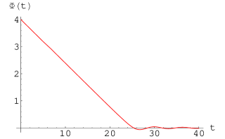
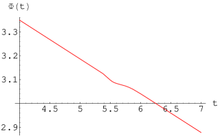
Figure 3: Time evolution of the inflaton field $\Phi(t)$ for the parameters (25). Time $t$ is measured in units of $M^{-1}$ and $\Phi$ is measured in units of $m_{Pl}$. In the left plot the slow-roll regime during inflation and the beginning of the inflaton oscillations are presented. The right plot shows the evolution of $\Phi$ in more detail near the point $\Phi=\Phi_{0}=3.1\,m_{Pl}$. The interaction of $\Phi$ with the field $\chi$ has a negligible effect on the inflation for the chosen parameters, so $\Phi(t)$ only slightly deviates from the straight line around $\Phi=\Phi_{0}$ (see the right plot).

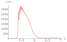
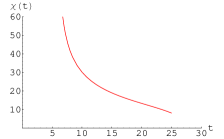
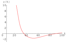
Figure 4: Time dependence of the field $\chi(t)$ for the parameters (25). Time $t$ is measured in units of $M^{-1}$ and $\chi$ is measured in units of $M$. All the three plots depict the evolution of $\chi$ during different time intervals. The left plot shows how the field $\chi$ rolls down to the minimum of the potential $\eta(t)>0$, oscillates there and then goes back to the newly formed minimum $\chi=0$. In the middle and right plots one can see that at the end of inflation, $t\approx 25\,M^{-1}$, the field $\chi$ remains quite large. Eventually $\chi$ crosses zero and slowly oscillates around $\chi=0$ (see the right plot).

In Fig. 4 one can see how the field $\chi$ rolls down to the minimum of the potential $\eta(t)>0$ and oscillates there. Then it goes back to the old minimum at $\chi=0$, but even at the end of inflation $\chi$ remains an order of magnitude larger than it was at the beginning ($\chi\sim 10\,M$ at $t\approx 25\,M^{-1}$, while $\chi_{in}=1\,M$). At the moment $t\approx 35\,M^{-1}$ the field $\chi$ crosses zero and starts slow oscillations with very low frequency, which could be much lower than the characteristic rate of baryogenesis.

So we see that parameters (25) are chosen in a proper way. In this model the influence of $\chi$ on the process of inflation is insignificant, thus the domain size grows exponentially. However, as we have mentioned at the end of the previous section, it is also important to know how the regions where $\chi=0$ expand during inflation. The hypothetical situation is possible when the areas where field is zero expand exponentially faster than the areas where field is non-zero. For example, the model where inflation never stops near the domain walls, i.e. near $\phi=0$, was suggested in linde . Also the idea of never ending topological inflation where $\phi$ is forced to stay near the maximum of its potential $\phi=0$ was proposed in vilenkin_1 ; vilenkin_2 . However, our situation is quite different. Numerical calculation shows that if $\chi=0$ the Hubble parameter remains almost the same as in the case of non-zero $\chi$, and the size of region where $\chi=0$ is approximately two times less than the domain size. Therefore, our model predicts the domains of cosmological size with the distances between them of the same order of magnitude.

IV Production of heavy particles after inflation and baryogenesis

As it is commonly known, the stage of inflation is followed by the stage of (re)heating, during which the very heavy $X$ particles can be produced through decay of inflaton field (see e.g. book Gorbunov ) or from vacuum fluctuations in gravitational field KT .

Let us consider the situation when the inflaton field $\Phi$ interacts with $X$ particles (for example, scalar bosons) through the coupling $g^{2}_{X}\Phi^{2}X^{2}$. As is shown in Refs. brandenberger ; kls_1 ; kls_2 , the particle production can be strongly enhanced due to parametric resonance. For an unsuppressed production it is essential that the resonance is broad. The corresponding condition has the form:

$$g_{X}\Phi_{e}\gg M.$$ (26)

Here $M\simeq 10^{-6}m_{Pl}$ is the inflaton mass, and $\Phi_{e}\simeq m_{Pl}/\sqrt{4\pi}$ is the magnitude of the inflaton field at the end of inflation in our model. One can consider $\Phi_{e}$ also as the initial amplitude of the inflaton oscillations. The condition (26) is true for the wide range of coupling constant, $g_{X}\gg 4\cdot 10^{-6}$.

Because of resonance (26), very heavy $X$-bosons with masses even of GUT scale $m_{X}\sim(Mm_{Pl})^{1/2}\sim 10^{16}$ GeV can be produced under quite reasonable assumption $g_{X}\sim 1$ Gorbunov . Moreover in this case of comparatively large coupling constant $g_{X}\sim 1$ the decay of the inflaton field occurs very rapidly, during only one or few oscillations.

Let us assume that the produced $X$-bosons in turn decay into fermions, for example, into quark-quark and antiquark-antilepton pairs, $X\rightarrow qq$ and $X\rightarrow\bar{q}\bar{l}$, respectively. If the corresponding coupling constants are large enough, the $X$-bosons decay very quickly. Therefore, the field $\chi(t)$ may remain non-zero yet to the moment when $X$-bosons have been completely decayed, indeed $\chi\sim 2\,M\sim 10^{13}$ GeV at $t=30\,M^{-1}$ (see Fig. 4).

The field $\chi$ is real and pseudoscalar and interacts with the produced fermions as (cf. (11))

$$L_{\chi\psi\psi}=g_{kl}\chi\bar{\psi}^{k}i\gamma_{5}\psi^{l}=g_{kl}\chi(\bar{\psi}^{k}_{R}i\gamma_{5}\psi^{l}_{L}+\bar{\psi}^{k}_{L}i\gamma_{5}\psi^{l}_{R})=ig_{kl}\chi(\bar{\psi}^{k}_{L}\psi^{l}_{R}-\bar{\psi}^{k}_{R}\psi^{l}_{L}),$$ (27)

where $k$ and $l$ denote the fermion flavor (sum over repetitive indices is assumed), $\psi_{R}=((1+\gamma_{5})/2)\psi$, $\psi_{L}=((1-\gamma_{5})/2)\psi$. From the hermicity of the interaction it follows that $g_{kl}$ is real for $k=l$, and $g_{kl}=g^{*}_{lk}$ for $k\neq l$. Since $\chi$ is supposed to be electrically neutral, it interacts with quarks with the same electric charge, so $k$ and $l$ either run over $u,\,c,\,t$ or $d,\,s,\,b$ and there are no cross terms.

The Lagrangian of free fermions can be written as follows

$$L_{free}=\bar{\psi}^{k}i\hat{\partial}\psi^{k}-m_{\psi kl}\bar{\psi}^{k}\psi^{l}=\bar{\psi}^{k}_{R}i\hat{\partial}\psi^{k}_{R}+\bar{\psi}^{k}_{L}i\hat{\partial}\psi^{k}_{L}-m_{\psi kl}(\bar{\psi}^{k}_{R}\psi^{l}_{L}+\bar{\psi}^{k}_{L}\psi^{l}_{R}).$$ (28)

Therefore, the sum of $L_{free}$ and $L_{\chi\psi\psi}$ can be presented in matrix form as

$$L_{free}+L_{\chi\psi\psi}=\bar{\psi}_{R}i\hat{\partial}\psi_{R}+\bar{\psi}_{L}i\hat{\partial}\psi_{L}-(\bar{\psi}_{R}M_{\psi}\psi_{L}+\bar{\psi}_{L}M_{\psi}^{\dagger}\psi_{R}),$$ (29)

here $M_{\psi}=m_{\psi}+ig\chi$ is a non-Hermitian matrix, whereas $m_{\psi}$ and $g$ are Hermitian ones.

Using simultaneously two unitary transformations $\psi_{R}\rightarrow\psi^{\prime}_{R}=U_{R}\psi_{R}$ and $\psi_{L}\rightarrow\psi^{\prime}_{L}=U_{L}\psi_{L}$ one can always diagonalize the mass matrix in (29). Therefore, the interaction of fermions with pseudoscalar field $\chi$ can be ”rotated away” (the elements of transformation matrices $U_{R}$ and $U_{L}$ must depend on the magnitude of $\chi$ in this case), and the Lagrangian (29) takes the simple form

$$L^{\prime}_{free}=\bar{\psi}^{a}i\hat{\partial}\psi^{a}-m^{\prime}_{\psi ab}\bar{\psi}^{a}\psi^{b},$$ (30)

where $\psi^{a}$ and $\psi^{b}$ are the mass eigenstates and correspondingly $m^{\prime}_{\psi}$ is diagonal matrix with real diagonal elements.

Quite similarly one can transform into mass term the interaction of fermions with any scalar $g_{Skl}S\bar{\psi}^{k}\psi^{l}$ and pseudoscalar $g_{Pkl}P\bar{\psi}^{k}i\gamma_{5}\psi^{l}$ fields . However, the interaction of fermions with vector (gauge) boson $X$ remains the same under these transformations:

$$g_{Rkl}X_{\mu}\bar{\psi}_{R}^{k}\gamma^{\mu}\psi_{R}^{l}+g_{Lkl}X_{\mu}\bar{\psi}_{L}^{k}\gamma^{\mu}\psi_{L}^{l}\rightarrow g^{\prime}_{Rab}X_{\mu}\bar{\psi}^{a}_{R}\gamma^{\mu}\psi^{b}_{R}+g^{\prime}_{Lab}X_{\mu}\bar{\psi}^{a}_{L}\gamma^{\mu}\psi^{b}_{L},$$ (31)

here $g^{\prime}_{R}=U_{R}g_{R}U^{\dagger}_{R}$ and $g^{\prime}_{L}=U_{L}g_{L}U^{\dagger}_{L}$ are matrices of coupling constants in mass eigenstate basis, so $\psi^{a}$ describes $a$-th sort of fermion with definite mass. The constants $g^{\prime}_{ab}$ are complex in general case, and if there are at least three species of fermions, one cannot rotate away simultaneously all phases in complex matrices $g^{\prime}_{R,L}$ KM . The complexity of the coupling constants means that $CP$ is violated in the $X$-boson decays NW . The magnitude of this $CP$ violation depends on the value of the field $\chi$ through the matrices $U_{R,L}$ and coupling constants $g^{\prime}_{R,L}$. Since $\chi$ is essentially non-zero after the end of inflation and during baryogenesis, the $CP$-odd effects can be large enough.

We assume also that gauge interactions involve fermions with certain chirality, see (31), and thus these interactions break $C$-invariance.

$C$ and $CP$ violation is one of the necessary Sakharov conditions of generation of baryon asymmetry sakharov . The another one is baryon number violation, so one needs to assume also that in the decays of $X$-bosons the baryon number is not conserved. Let $\delta$ be the baryon asymmetry generated in the decay of one $X$-boson. Then it can be easily demonstrated Gorbunov that the ratio of the baryon number density to the entropy density is estimated as

$$\Delta_{B}=\frac{n_{B}-n_{\bar{B}}}{s}\sim\delta\frac{h}{g_{X}}\left(\frac{m_{th}}{m_{Pl}}\right)^{1/2},$$ (32)

where $h$ and $g_{X}$ are typical coupling constants of $X$-boson with fermions and inflaton, respectively, $m_{th}$ is mass scale of the theory. It is quite reasonable to believe that $h/g_{X}\sim 1$ and $m_{th}\sim M\sim 10^{-6}\,m_{Pl}$, so one has $\Delta_{B}\sim 10^{-3}\delta$. Thus, to get observed value $\Delta_{B}\simeq 0.86\cdot 10^{-10}$ it is sufficient to have only $\delta\sim 10^{-7}$. Such small $\delta$ seems to be easily produced in the decay of $X$-boson. Therefore, the observed baryon asymmetry of the universe can be generated in the decays of $X$-bosons, without fine tuning of parameters of the theory.

We have to stress that the baryogenesis should proceed after the end of inflation (as it has been already mentioned above). Otherwise the baryon asymmetry would be strongly diluted by the universe (re)heating. When inflation was over, the field $\chi$ evolved down to $\chi=0$ and so $\chi$ was not equal to constant $\eta$ but had considerably smaller and time dependent value. However, since at this stage $\chi(t)$ changed very slowly one can repeat the above arguments with adiabatically evolving $\chi(t)$. If baryogenesis proceeded faster than $\chi$ evolved, then the effective amplitude of $CP$ violation might be considered as a constant and the corresponding mass matrix could be diagonalized in the same way as it has been done above. The phase of the mass matrix would be unsuppressed if $g\chi(t)$ was close to the value of the bare quark mass. Evidently in this case the imaginary part of the mass matrix would be of the same order of magnitude as the real part.

V Conclusions

We have presented here a model of baryogenesis which may lead to baryo-symmetric universe with cosmologically large domains of matter and antimatter, avoiding the domain wall problem. The model satisfies three Sakharov criteria for successful baryogenesis: non-conservation of the baryon number, deviation from thermal equilibrium, and $C$ and $CP$ violation. However, the latter is different from the normally exploited one. Breaking of charge symmetry is induced by a non-zero amplitude of a scalar field $\chi$, which slowly relaxed down to equilibrium, much slower than the process of baryogenesis goes on. In classification of different types of $CP$ violation which might be operative in cosmology this type is called dynamical one AD-Varenna . Later, after the baryon asymmetry was developed, $\chi$ evolved down to the equilibrium point $\chi=0$ and thus domain walls disappeared rather early in the universe.

Inflation is an essential ingredient of the scenario. A coupling to the inflaton field was introduced on purpose to generate a non-zero value of $\chi$ and to keep it non-zero during baryogenesis.

The model allows for successful baryo-symmetric cosmology without yet being drawn into astronomical controversy.

References

- (1) A.D. Dolgov, NonGUT baryogenesis, Phys. Rept. 222 (1992) 309.
- (2) A.D. Dolgov, Baryogenesis, 30 years after, Surv. High Energ. Phys. 13 (1998) 83 [hep-ph/9707419].
- (3) V.A. Rubakov and M.E. Shaposhnikov, Electroweak baryon number nonconservation in the early universe and in high-energy collisions, Phys. Usp. 39 (1996) 461 [Usp. Fiz. Nauk 166 (1996) 493] [hep-ph/9603208].
- (4) A. Riotto and M. Trodden, Recent progress in baryogenesis, Ann. Rev. Nucl. Part. Sci. 49 (1999) 35 [hep-ph/9901362].
- (5) M. Dine and A. Kusenko, The origin of the matter-antimatter asymmetry, Rev. Mod. Phys. 76 (2003) 1 [hep-ph/0303065].
- (6) A.G. Cohen, A. De Rujula and S.L. Glashow, A matter-antimatter universe?, Astrophys. J. 495 (1998) 539 [astro-ph/9707087].
- (7) Ya. B. Zeldovich, I.Yu. Kobzarev and L.B. Okun, Cosmological Consequences of the Spontaneous Breakdown of Discrete Symmetry, Zh. Eksp. Teor. Fiz. 67 (1974) 3 [Sov. Phys. JETP 40 (1974) 1].
- (8) V.A. Kuzmin, I.I. Tkachev and M.E. Shaposhnikov, Are There Domains of Antimatter in the Universe? (in Russian), Pisma Zh. Eksp. Teor. Fiz. 33 (1981) 557.
- (9) V.A. Kuzmin, M.E. Shaposhnikov and I.I. Tkachev, Gauge Hierarchies and Unusual Symmetry Behavior at High Temperatures, Phys. Lett. B 105 (1981) 159.
- (10) V.A. Kuzmin, M.E. Shaposhnikov and I.I. Tkachev, Matter-Antimatter Domains in the Universe: A Solution of the Vacuum Walls Problem, Phys. Lett. B 105 (1981) 167.
- (11) V.A. Kuzmin, M.E. Shaposhnikov and I.I. Tkachev, Baryon generation and unusual symmetry behaviour at high temperatures, Nucl. Phys. B 196 (1982) 29.
- (12) S.I. Blinnikov, A.D. Dolgov and K.A. Postnov, Antimatter and antistars in the universe and in the Galaxy, Phys. Rev. D 92 (2015) 023516 [arXiv:1409.5736].
- (13) F.W. Stecker, The matter-antimatter asymmetry of the universe, in the proceedings of 14th Rencontres de Blois on Matter-Antimatter Asymmetry, Chateau de Blois, France, June 17-22, 2002 [hep-ph/0207323].
- (14) A.D. Dolgov, Cosmological matter antimatter asymmetry and antimatter in the universe, in the proceedings of 14th Rencontres de Blois on Matter-Antimatter Asymmetry, Chateau de Blois, France, June 17-22, 2002 [hep-ph/0211260].
- (15) S.E. Larsson, S. Sarkar and P.L. White, Evading the cosmological domain wall problem, Phys. Rev. D 55 (1997) 5129 [hep-ph/9608319].
- (16) M. Kobayashi and T. Maskawa, CP Violation in the Renormalizable Theory of Weak Interaction, Prog. Theor. Phys. 49 (1973) 652.
- (17) A.D. Linde, Monopoles as big as a universe, Phys. Lett. B 327 (1994) 208 [astro-ph/9402031].
- (18) R. Basu and A. Vilenkin, Evolution of topological defects during inflation, Phys. Rev. D 50 (1994) 7150 [gr-qc/9402040].
- (19) A. Vilenkin, Topological inflation, Phys. Rev. Lett. 72 (1994) 3137 [hep-th/9402085].
- (20) D.S. Gorbunov, V.A. Rubakov, Introduction to the theory of the early universe: Cosmological perturbations and inflationary theory, World Scientific (2011).
- (21) V.A. Kuzmin and I.I. Tkachev, Matter creation via vacuum fluctuations in the early universe and observed ultrahigh-energy cosmic ray events, Phys. Rev. D 59 (1999) 123006 [hep-ph/9809547].
- (22) Yu.V. Shtanov, J.H. Traschen and R.H. Brandenberger, Universe reheating after inflation, Phys. Rev. D 51 (1995) 5438 [hep-ph/9407247].
- (23) L. Kofman, A.D. Linde and A.A. Starobinsky, Reheating after inflation, Phys. Rev. Lett. 73 (1994) 3195 [hep-th/9405187].
- (24) L. Kofman, A.D. Linde and A.A. Starobinsky, Towards the theory of reheating after inflation, Phys. Rev. D 56 (1997) 3258 [hep-ph/9704452].
- (25) D.V. Nanopoulos and S. Weinberg, Mechanisms for Cosmological Baryon Production, Phys. Rev. D 20 (1979) 2484.
- (26) A.D. Sakharov, Violation of CP Invariance, C Asymmetry and Baryon Asymmetry of the Universe, JETP Lett. 5 (1967) 24 [Pisma Zh. Eksp. Teor. Fiz. 5 (1967) 32], Sov. Phys. Usp. 34 (1991) 392 [Usp. Fiz. Nauk 161 (1991) 61].
- (27) A.D. Dolgov, CP violation in cosmology, in the proceedings of 163rd Course of International School of Physics ’Enrico Fermi’: CP Violation: From Quarks to Leptons, Varenna, Italy, July 19-29, 2005 [hep-ph/0511213].