Mapping gravitational-wave backgrounds in modified theories of gravity using pulsar timing arrays

Abstract

We extend our previous work on applying CMB techniques to the mapping of gravitational-wave backgrounds to backgrounds which have non-GR polarisations. Our analysis and results are presented in the context of pulsar-timing array observations, but the overarching methods are general, and can be easily applied to LIGO or eLISA observations using appropriately modified response functions. Analytic expressions for the pulsar-timing response to gravitational waves with non-GR polarisation are given for each mode of a spin-weighted spherical-harmonic decomposition of the background, which permit the signal to be mapped across the sky to any desired resolution. We also derive the pulsar-timing overlap reduction functions for the various non-GR polarisations, finding analytic forms for anisotropic backgrounds with scalar-transverse (“breathing”) and vector-longitudinal polarisations, and a semi-analytic form for scalar-longitudinal backgrounds. Our results indicate that pulsar-timing observations will be completely insensitive to scalar-transverse mode anisotropies in the polarisation amplitude beyond dipole, and anisotropies in the power beyond quadrupole. Analogously to our previous findings that pulsar-timing observations lack sensitivity to tensor-curl modes for a transverse-traceless tensor background, we also find insensitivity to vector-curl modes for a vector-longitudinal background.

I Introduction

A massive international effort is currently underway to observe gravitational waves across a wide range of frequencies. The second-generation of ground-based gravitational-wave interferometers are about to start collecting data, with Advanced LIGO Harry et al. (2010) observation runs expected to begin before the end of 2015. The two Advanced LIGO detectors will form part of a global network of kilometre-scale laser interferometers, with other instruments due to come online during the rest of this decade. These detectors will employ advanced technologies to detect gravitational waves from stellar-mass compact binary systems emitting gravitational radiation in the kHz band Somiya (2012); Unnikrishnan (2013); GEO ; Adv (2009). The European Space Agency recently selected a science theme based around a $\sim\!10^{9}~{}{\rm m}$ arm-length space-based gravitational-wave interferometer (eLISA) for the L$3$ mission slot, due to launch in 2034. Such a detector will observe gravitational waves in the millihertz band, which are generated by binaries involving the massive black holes that reside in the centres of galaxies, with mass about one million times the mass of the Sun. These observations will permit tests of fundamental physics to exquisite precision, whilst also affording detailed demographic studies of massive black-hole populations Amaro-Seoane et al. (2012).

Complementary to these experiments are ongoing efforts to characterise nanohertz gravitational waves through their perturbation to the arrival-times of radio signals from precisely timed ensembles of millisecond pulsars spread throughout our galaxy van Haasteren et al. (2011); Demorest et al. (2013); Shannon et al. (2013); Manchester and IPTA (2013). As a gravitational wave transits between the Earth and a pulsar, it induces a change in their proper separation, leading to a redshift in the arrival rate of the pulsar signals Sazhin (1978); Detweiler (1979); Estabrook and Wahlquist (1975); Burke (1975). It is the exceptional stability of the integrated pulse profiles of millisecond pulsars, and the resulting accuracy of the models for the pulse times of arrival (TOAs), that allow gravitational waves to be detected in this way.

The differences between the modelled TOAs and the actual observed TOAs are known as the timing residuals. These residuals contain the influence of all unmodelled phenomena, such as additional receiver noise, interstellar medium effects, errors resulting from drifts in clock standards or ephemeris inaccuracies, and, most tantalisingly, gravitational radiation. The signature of gravitational waves in these residuals may be deterministic or stochastic. The gravitational-wave sources expected to dominate the signal in the nanohertz frequency band are the early adiabatic inspirals of supermassive black-hole binary (SMBHB) systems Rajagopal and Romani (1995); Jaffe and Backer (2003); Wyithe and Loeb (2003). Such systems are expected to form following the (suspected ubiquitous) mergers of massive galaxies during the hierarchical formation of structure. If there is a system which is particularly loud in gravitational-wave emission then this signal may be individually resolved and detected with pipelines dedicated to searches for the deterministic signals of single sources Ellis et al. (2012); Ellis (2013); Taylor et al. (2014). If, however, there are many sources which pile up in the frequency-domain beyond the ability of our techniques to separately resolve them, then the combined signal will form a stochastic background of gravitational waves. Although there are other mechanisms which may contribute to a stochastic nHz gravitational-wave background (decay of cosmic-string networks Vilenkin (1981a, b); Ölmez et al. (2010); Sanidas et al. (2012) or primordial remnants Grishchuk (1976, 2005)), this incoherent superposition of signals from many SMBHB systems is expected to dominate the signal.

Standard pipelines in use today employ cross-correlation techniques to search for stochastic backgrounds. The presence of a common background of gravitational waves affecting the TOAs of all pulsars in an array (a so-called pulsar-timing array, PTA Foster and Backer (1990)) makes a cross-correlation search effective in leveraging the signal against uncorrelated noise processes. The concept of an overlap reduction function is common to stochastic background searches for all types of gravitational-wave detectors, and describes the sky-averaged overlap of the antenna pattern functions of the two detectors whose data are being correlated Flanagan (1993). In PTA analysis, the overlap reduction function for a Gaussian, stationary, unpolarised, isotropic stochastic background composed of transverse-traceless (TT) gravitational-wave modes is a smoking-gun signature of the signal, known as the Hellings and Downs curve Hellings and Downs (1983). It is a function of one variable: the angular separation between a pair of pulsars.

For anisotropic distributions of gravitational-wave power on the sky, the overlap reduction function is no longer merely a function of the pulsars’ angular-separation. It will also depend on the positions of the pulsars on the sky relative to the distribution of gravitational-wave power, and thus will be a rich source of information in the precision-science-era of PTAs Mingarelli et al. (2013); Taylor and Gair (2013). Furthermore, the overlap reduction function can be shown to vary when describing backgrounds where the graviton is permitted to have a small but non-zero mass Lee (2014). The same is true when describing the overlap reduction functions induced by gravitational-wave polarisation states present in modified (metric) theories of gravity. In addition to the usual GR transverse-traceless tensor polarisation states, the beyond-GR polarisations consist of a scalar-transverse (“breathing”) state, a scalar-longitudinal state, and two vector-longitudinal states, each inducing correlation signatures which are markedly distinct from the Hellings and Downs curve Lee et al. (2008); Chamberlin and Siemens (2012).

In this paper we focus on the response of pulsar timing observations to gravitational wave backgrounds with non-GR polarisation states. By decomposing a background of given polarisation in terms of spin-weighted spherical harmonics, we are able to derive analytic expressions for the detector response functions for each mode of each non-GR polarisation state as a function of the harmonic multipole. We discuss the implications of these results for mapping non-GR backgrounds to any desired angular resolution. We are also able to present analytic expressions for the overlap reduction functions of anisotropic scalar-transverse and vector-longitudinal backgrounds, whilst significant analytic headway is made for the corresponding function for scalar-longitudinal backgrounds.

In Sec. II we introduce the concept of the measured signal in a gravitational-wave detector being a convolution of the metric perturbations with the response tensor of the detector. We discuss the six distinct polarisation states of gravitational waves which are permitted within a general metric theory of gravity by virtue of obeying Einstein’s Equivalence Principle. The basis tensors for these polarisations are explicitly given. We also discuss the decomposition of the metric perturbations in terms of appropriate spin-weighted spherical harmonics. In Gair et al. (2014), the Fourier amplitudes of a plane-wave expansion of the metric perturbations for an arbitrary transverse-traceless gravitational-wave background were decomposed in terms of a basis of spin-weight $\pm 2$ spherical harmonics. In the case of scalar-transverse and scalar-longitudinal polarisations discussed in this paper, we decompose the Fourier amplitudes in terms of ordinary (spin-weight $0$) spherical harmonics. For the vector-longitudinal polarisations, we decompose the Fourier amplitudes in terms of spin-weight $\pm 1$ spherical harmonics. In Sec. II, we also give expressions for the pulsar timing response functions, for either the polarisation or spin-weighted spherical harmonic expansion coefficients. The polarisation basis response functions for a pair of pulsars are given explicitly in the computational frame, where one pulsar lies along the $z$-axis and the other lies in the $xz$-plane. These are needed for the overlap reduction functions calculations given in the following section.

The overlap reduction functions for the different polarisation states are studied in Sec. III. This function describes the response of a pair of pulsars to a gravitational-wave background in a cross-correlation analysis, and is computed by integrating the overlap of the response of each pulsar to a particular gravitational-wave polarisation over the entire sky. For a gravitational-wave background with arbitrary angular structure, this sky integral must be weighted by the gravitational-wave power at each sky location. We find an analytic expression for the overlap reduction function for a background with scalar-transverse (breathing) polarisation, and show that a PTA will lack sensitivity to angular structure beyond quadrupole in a cross-correlation analysis for this type of background. We also make significant analytic headway for the overlap reduction function of a scalar-longitudinal background, and find analytic forms for the limiting value in the case of co-directional and anti-directional pulsars. The overlap reduction function for a vector-longitudinal background with arbitrary angular structure is found analytically, with superficially perceived divergences in the overlap reduction function for co-directional pulsars resolved by correctly incorporating the pulsar term in our calculations.

In Sec. IV we extend our previous work on mapping gravitational-wave backgrounds using CMB techniques (Gair et al., 2014) to non-GR polarisations. We derive analytic expressions for the response of a pulsar to each mode (corresponding to a particular spin-weighted spherical harmonic) of the background, including the contribution from the pulsar term. In the process of doing these calculations, we find that the reason for the PTA insensitivity to angular structure beyond quadrupole in the gravitational-wave power of a scalar-transverse background is due entirely to the corresponding lack of sensitivity of a single pulsar response to structure in the polarisation amplitudes beyond dipole. We verify this analytic result with numerical map making and recovery. The pulsar response to individual modes of a scalar-longitudinal and vector-longitudinal background are given analytically, where in the latter case we find that PTAs completely lack sensitivity to vector curl modes, analogous to our previous finding that PTAs lack sensitivity to tensor curl modes of a transverse-traceless background (Gair et al., 2014). We discuss these findings further in Sec. V, along with suggestions for future study and implications for the forthcoming analysis of real PTA data.

Finally, we include several appendices (Apps. A–L), containing relevant information (e.g., definitions, identities, recurrence relations) for spin-weighted and tensor spherical harmonics, Legendre polynomials, Bessel functions, etc., as well as providing technical details for the overlap reduction function and response function calculations described in Secs. III and IV.

II Response functions

II.1 Detector response

The response of a detector to a passing gravitational wave is given by the convolution of the metric perturbations $h_{ab}(t,\vec{x})$ with the impulse response $R^{ab}(t,\vec{x})$ of the detector:

$$r(t)=\int_{-\infty}^{\infty}{\rm d}\tau\int{\rm d}^{3}y\>R^{ab}(\tau,\vec{y})h_{ab}(t-\tau,\vec{x}-\vec{y})\,.$$ (1)

If we write the metric perturbations as a superposition of plane waves

$$h_{ab}(t,\vec{x})=\int_{-\infty}^{\infty}{\rm d}f\int_{S^{2}}{\rm d}^{2}\Omega_{\hat{k}}\>h_{ab}(f,\hat{k})e^{i2\pi f(t-\hat{k}\cdot\vec{x}/c)}\,,$$ (2)

then

$$r(t)=\int_{-\infty}^{\infty}{\rm d}f\int_{S^{2}}{\rm d}^{2}\Omega_{\hat{k}}\>R^{ab}(f,\hat{k})h_{ab}(f,\hat{k})e^{i2\pi ft}\,,$$ (3)

where

$$R^{ab}(f,\hat{k})=e^{-i2\pi f\hat{k}\cdot\vec{x}/c}\\ \times\int_{-\infty}^{\infty}{\rm d}\tau\int{\rm d}^{3}y\>R^{ab}(\tau,\vec{y})\,e^{-i2\pi f(\tau-\hat{k}\cdot\vec{y}/c)}\,.$$ (4)

Further specification of the response function depends on the choice of gravitational-wave detector as well as on the basis tensors used to expand $h_{ab}(f,\hat{k})$, as we explain below.

II.2 Polarisation basis

In standard GR, the Fourier components $h_{ab}(f,\hat{k})$ are typically expanded in terms of the $+$ and $\times$ polarisation basis tensors:

$$h_{ab}(f,\hat{k})=h_{+}(f,\hat{k})e^{+}_{ab}(\hat{k})+h_{\times}(f,\hat{k})e^{\times}_{ab}(\hat{k})\,,$$ (5)

where

$$e_{ab}^{+}(\hat{k}) =\hat{\theta}_{a}\hat{\theta}_{b}-\hat{\phi}_{a}\hat{\phi}_{b},$$ (6)

$$e_{ab}^{\times}(\hat{k}) =\hat{\theta}_{a}\hat{\phi}_{b}+\hat{\phi}_{a}\hat{\theta}_{b},$$

and $\hat{\theta}$, $\hat{\phi}$ are the standard unit vectors tangent to the sphere:

$$\hat{k} =\sin\theta\cos\phi\,\hat{x}+\sin\theta\sin\phi\,\hat{y}+\cos\theta\,\hat{z}\,,$$ (7)

$$\hat{\theta} =\cos\theta\cos\phi\,\hat{x}+\cos\theta\sin\phi\,\hat{y}-\sin\theta\,\hat{z}\,,$$

$$\hat{\phi} =-\sin\phi\,\hat{x}+\cos\phi\,\hat{y}\,.$$

In this paper, we also consider modified metric theories of gravity, which admit four other types of polarisation: a scalar-transverse (or breathing) mode ($B$), a scalar-longitudinal mode ($L$), and two vector-longitudinal modes ($X$, $Y$). The polarisation basis tensors for these modes are:

$$e_{ab}^{B}(\hat{k}) =\hat{\theta}_{a}\hat{\theta}_{b}+\hat{\phi}_{a}\hat{\phi}_{b}\,,$$ (8)

$$e_{ab}^{L}(\hat{k}) =\sqrt{2}\,\hat{k}_{a}\hat{k}_{b}\,,$$ (9)

$$e_{ab}^{X}(\hat{k}) =\hat{\theta}_{a}\hat{k}_{b}+\hat{k}_{a}\hat{\theta}_{b}\,,$$ (10)

$$e_{ab}^{Y}(\hat{k}) =\hat{\phi}_{a}\hat{k}_{b}+\hat{k}_{a}\hat{\phi}_{b}\,.$$ (11)

In terms of the polarisation tensors, the Fourier components $h_{ab}(f,\hat{k})$ can be expanded generally as

$$h_{ab}(f,\hat{k})=\sum_{A}h_{A}(f,\hat{k})e^{A}_{ab}(\hat{k})$$ (12)

where $A$ is some subset of $\{+,\times,B,L,X,Y\}$. The associated response function for a plane wave with frequency $f$, propagation direction $\hat{k}$, and polarisation $A$ is given by

$$R^{A}(f,\hat{k})=R^{ab}(f,\hat{k})e^{A}_{ab}(\hat{k})\,,$$ (13)

and is related to the detector response $r(t)$ via:

$$r(t)=\int_{-\infty}^{\infty}{\rm d}f\int_{S^{2}}{\rm d}^{2}\Omega_{\hat{k}}\sum_{A}R^{A}(f,\hat{k})h_{A}(f,\hat{k})e^{i2\pi ft}\,.$$ (14)

We will work with the polarisation basis response functions when calculating the various overlap reduction functions in Sec. III.

II.3 Spherical harmonic basis

Alternatively, we can expand the Fourier components $h_{ab}(f,\hat{k})$ in terms of the appropriate spin-weighted spherical harmonics, as was done in Gair et al. (2014). A spin-weighted function is a function of both position on the sphere, labelled $\hat{k}$, and of a choice of an orthonormal basis, labelled $\hat{l},\hat{m}$, at points on the sphere. Under a rotation of the orthonormal basis, spin-weight functions transform in a particular way

$$f(\hat{k},\cos\psi\hat{l}-\sin\psi\hat{m},\sin\psi\hat{l}+\cos\psi\hat{m})={\rm e}^{is\psi}f(\hat{k},\hat{l},\hat{m})$$ (15)

where $s$ is the spin-weight of the function. Any spin-weight $s$ function can be expanded as a combination of spin-weighted spherical harmonics of the same weight, ${}_{s}Y_{lm}(\hat{k})$. A spin-weight $s$ spherical-harmonic can be related to $s$ derivatives of an ordinary spherical harmonic, as described in App. A.

For the standard GR tensor modes, if we define $\hat{m}_{\pm}^{a}=\hat{l}^{a}\pm i\hat{m}^{a}$, we see that the combinations $\hat{m}_{\pm}^{a}\hat{m}_{\pm}^{b}h_{ab}(f,\hat{k})$are spin-weight $\pm 2$ functions on the sphere. This allows the GR tensor modes to be expanded as combinations of spin-weight $\pm 2$ spherical harmonics, or equivalently in terms of the rank-2 gradient and curl spherical harmonics, $Y^{G}_{(lm)ab}(\hat{k})$, $Y^{C}_{(lm)ab}(\hat{k})$, defined by Eq. (111) in App. C:

$$h_{ab}(f,\hat{k})=\sum_{l=2}^{\infty}\sum_{m=-l}^{l}\left[a^{G}_{(lm)}(f)Y^{G}_{(lm)ab}(\hat{k})\right.\\ \left.+a^{C}_{(lm)}(f)Y^{C}_{(lm)ab}(\hat{k})\right]\,.$$ (16)

For the breathing and scalar-longitudinal modes, the functions $\hat{m}_{\pm}^{a}\hat{m}_{\pm}^{b}h_{ab}(f,\hat{k})$ are spin-weight $0$ and so we can expand $h_{ab}(f,\hat{k})$ in terms of ordinary (scalar) spherical harmonics:

$$h_{ab}(f,\hat{k}) =\frac{1}{\sqrt{2}}\sum_{l=0}^{\infty}\sum_{m=-l}^{l}a^{B}_{(lm)}(f)Y_{lm}(\hat{k})e^{B}_{ab}(\hat{k})\,,$$ (17)

$$h_{ab}(f,\hat{k}) =\frac{1}{\sqrt{2}}\sum_{l=0}^{\infty}\sum_{m=-l}^{l}a^{L}_{(lm)}(f)Y_{lm}(\hat{k})e^{L}_{ab}(\hat{k})\,,$$ (18)

since the polarisation tensors $e^{B}_{ab}(\hat{k})$ and $e^{L}_{ab}(\hat{k})$ are invariant under a rotation of $\hat{\theta}$, $\hat{\phi}$. For the vector-longitudinal modes, $\hat{m}_{\pm}^{a}\hat{m}_{\pm}^{b}h_{ab}(\hat{k})$ have spin-weight $\pm 1$ and so we can expand $h_{ab}(f,\hat{k})$ in terms of spin-weight $\pm 1$ spherical harmonics or, equivalently, in terms of tensor fields $Y^{V_{G}}_{(lm)ab}(\hat{k})$, $Y^{V_{C}}_{(lm)ab}(\hat{k})$ constructed from the rank-1 vector spherical harmonics $Y^{G}_{(lm)a}(\hat{k})$, $Y^{C}_{(lm)a}(\hat{k})$ defined by Eqs. (100) and (108) in App. B:

$$h_{ab}(f,\hat{k})=\sum_{l=1}^{\infty}\sum_{m=-l}^{l}\left[a^{V_{G}}_{(lm)}(f)Y^{V_{G}}_{(lm)ab}(\hat{k})\right.\\ \left.+a^{V_{C}}_{(lm)}(f)Y^{V_{C}}_{(lm)ab}(\hat{k})\right]\,.$$ (19)

The above expressions for $h_{ab}(f,\hat{k})$ can be written in compact form

$$h_{ab}(f,\hat{k})=\sum_{(lm)}\sum_{P}a_{(lm)}^{P}(f)Y^{P}_{(lm)ab}(\hat{k})$$ (20)

if we take $P$ to be a subset of $\{G,C,B,L,V_{G},V_{C}\}$, and define

$$Y^{B,L}_{(lm)ab}(\hat{k})\equiv\frac{1}{\sqrt{2}}Y_{lm}(\hat{k})e^{B,L}_{ab}(\hat{k})$$ (21)

to unify the notation for the spherical harmonic basic tensors. (The factor of $1/\sqrt{2}$ is needed for the tensor spherical harmonics $Y^{B,L}_{(lm)ab}(\hat{k})$ to satisfy orthonormality relations similar to Eqs. (110) and (118).) The associated response function for a given spherical harmonic mode is

$$R^{P}_{(lm)}(f)=\int_{S^{2}}{\rm d}^{2}\Omega_{\hat{k}}\>R^{ab}(f,\hat{k})Y^{P}_{(lm)ab}(\hat{k})\,,$$ (22)

and are related to the detector response $r(t)$ via:

$$r(t)=\int_{-\infty}^{\infty}{\rm d}f\sum_{(lm)}\sum_{P}R^{P}_{(lm)}(f)a^{P}_{(lm)}(f)e^{i2\pi ft}\,.$$ (23)

We will work with these response functions for the mapping discussion in Sec. IV.

II.4 Pulsar timing response

A gravitational wave transiting an Earth-pulsar line of sight creates a perturbation in the intervening metric. This causes a change in their proper separation, which is manifested as a redshift in the pulse frequency Sazhin (1978); Detweiler (1979); Estabrook and Wahlquist (1975); Burke (1975):

$$z(t,\hat{k})\equiv\frac{\Delta v(t)}{\nu_{0}} = \frac{1}{2}\frac{u^{a}u^{b}}{1+\hat{k}\cdot\hat{u}}\Delta h_{ab}(t,\hat{k})\,,$$ (24)

where $\hat{k}$ is the direction of propagation of the gravitational wave, $\hat{u}$ is the direction to the pulsar, and $\Delta h_{ab}(t,\hat{k})$ is the difference between the metric perturbation at Earth, $(t,\vec{x})$, and at the pulsar some distance $L$ from the Earth, $(t_{p},\vec{x}_{p})=(t-L/c,\vec{x}+L\hat{u})$:

$$\Delta h_{ab}(t,\hat{k}) \equiv\int_{-\infty}^{\infty}{\rm d}f\>\sum_{A}h_{A}(f,\hat{k})e^{A}_{ab}(\hat{k})\left[e^{i2\pi f(t-\hat{k}\cdot\vec{x}/c)}-e^{i2\pi f(t_{p}-\hat{k}\cdot\vec{x}_{p}/c)}\right]$$ (25)

$$=\int_{-\infty}^{\infty}{\rm d}f\>\sum_{A}h_{A}(f,\hat{k})e^{A}_{ab}(\hat{k})e^{i2\pi f(t-\hat{k}\cdot\vec{x}/c)}\left[1-e^{-i2\pi fL(1+\hat{k}\cdot\hat{u})/c}\right]\,.$$ (26)

For a gravitational wave background, which is a superposition of waves from all directions on the sky, the pulsar redshift integrated over $\hat{k}$ is given by

$$z(t)=\int_{-\infty}^{\infty}{\rm d}f\int_{S^{2}}{\rm d}^{2}\Omega_{\hat{k}}\sum_{A}\frac{1}{2}\frac{u^{a}u^{b}}{1+\hat{k}\cdot\hat{u}}e_{ab}^{A}(\hat{k})\left[1-e^{-i2\pi fL(1+\hat{k}\cdot\hat{u})/c}\right]h_{A}(f,\hat{k})e^{i2\pi f(t-\hat{k}\cdot\vec{x}/c)}\,.$$ (27)

Comparing the above expression with Eq. (14), we see that the detector response function $R^{A}(f,\hat{k})$ for a Doppler frequency measurement $r(t)\equiv z(t)$ is given by

$$R^{A}(f,\hat{k})=\frac{1}{2}\frac{u^{a}u^{b}}{1+\hat{k}\cdot\hat{u}}e_{ab}^{A}(\hat{k})e^{-i2\pi f\hat{k}\cdot\vec{x}}\left[1-e^{-i2\pi fL(1+\hat{k}\cdot\hat{u})/c}\right]\,.$$ (28)

For a timing residual measurement $r(t)\equiv\int_{0}^{t}dt^{\prime}\>z(t^{\prime})$, the above response function $R^{A}(f,\hat{k})$ would need to be multiplied by a factor of $1/(i2\pi f)$. The response functions for individual spherical harmonic modes are similarly given by

$$R^{P}_{(lm)}(f)=\int_{S^{2}}{\rm d}^{2}\Omega_{\hat{k}}\>\frac{1}{2}\frac{u^{a}u^{b}}{1+\hat{k}\cdot\hat{u}}Y_{(lm)ab}^{P}(\hat{k})e^{-i2\pi f\hat{k}\cdot\vec{x}}\left[1-e^{-i2\pi fL(1+\hat{k}\cdot\hat{u})/c}\right]\,.$$ (29)

II.5 Response functions for a pair of pulsars in the computational frame

In the following section, we will calculate the correlated response of a pair of pulsars to a gravitational wave background. This calculation is most easily done in the so-called computational frame (Allen and Ottewill, 1997; Mingarelli et al., 2013; Gair et al., 2014), in which the two pulsars are in the directions

$$\hat{u}_{1} =(0,0,1)\,,$$ (30)

$$\hat{u}_{2} =(\sin\zeta,0,\cos\zeta)\,.$$

In addition, we can choose the origin of the computational frame to be at the solar-system barycentre (SSB), for which a detector (i.e., a radio telescope on Earth) has $\vec{x}\approx\vec{0}$. In this frame the polarisation basis response functions given in Eq. (28) simplify to

$$R^{+}_{1}(f,\hat{k}) =\frac{1}{2}(1-\cos\theta)\left(1-{\rm e}^{-2\pi ifL_{1}(1+\cos\theta)/c}\right)\,,$$ (31)

$$R^{+}_{2}(f,\hat{k}) =\frac{1}{2}\left[(1-\sin\zeta\sin\theta\cos\phi-\cos\theta\cos\zeta)-\frac{2\sin^{2}\zeta\sin^{2}\phi}{1+\sin\zeta\sin\theta\cos\phi+\cos\theta\cos\zeta}\right]$$

$$\hskip 113.81102pt\times\left(1-{\rm e}^{-2\pi ifL_{2}(1+\sin\zeta\sin\theta\cos\phi+\cos\theta\cos\zeta)/c}\right)\,,$$ (32)

$$R^{\times}_{1}(f,\hat{k}) =0\,,$$ (33)

$$R^{\times}_{2}(f,\hat{k}) =-\frac{1}{2}\left(\frac{\sin^{2}\zeta\cos\theta\sin(2\phi)-\sin(2\zeta)\sin\theta\sin\phi}{1+\sin\zeta\sin\theta\cos\phi+\cos\theta\cos\zeta}\right)\left(1-{\rm e}^{-2\pi ifL_{2}(1+\sin\zeta\sin\theta\cos\phi+\cos\theta\cos\zeta)/c}\right)\,,$$ (34)

$$R^{B}_{1}(f,\hat{k}) =\frac{1}{2}(1-\cos\theta)\left(1-{\rm e}^{-2\pi ifL_{1}(1+\cos\theta)/c}\right)\,,$$ (35)

$$R^{B}_{2}(f,\hat{k}) =\frac{1}{2}(1-\sin\zeta\sin\theta\cos\phi-\cos\theta\cos\zeta)\left(1-{\rm e}^{-2\pi ifL_{2}(1+\sin\zeta\sin\theta\cos\phi+\cos\theta\cos\zeta)/c}\right)\,,$$ (36)

$$R^{L}_{1}(f,\hat{k}) =\frac{1}{\sqrt{2}}\frac{\cos^{2}\theta}{1+\cos\theta}\left(1-{\rm e}^{-2\pi ifL_{1}(1+\cos\theta)/c}\right)\,,$$ (37)

$$R^{L}_{2}(f,\hat{k}) =\frac{1}{\sqrt{2}}\frac{(\sin\zeta\sin\theta\cos\phi+\cos\theta\cos\zeta)^{2}}{1+\sin\zeta\sin\theta\cos\phi+\cos\theta\cos\zeta}\left(1-{\rm e}^{-2\pi ifL_{2}(1+\sin\zeta\sin\theta\cos\phi+\cos\theta\cos\zeta)/c}\right)\,,$$ (38)

$$R^{X}_{1}(f,\hat{k}) =\frac{-\cos\theta\sin\theta}{1+\cos\theta}\left(1-{\rm e}^{-2\pi ifL_{1}(1+\cos\theta)/c}\right)\,,$$ (39)

$$R^{X}_{2}(f,\hat{k}) =\frac{(\sin\zeta\sin\theta\cos\phi+\cos\theta\cos\zeta)(\sin\zeta\cos\theta\cos\phi-\sin\theta\cos\zeta)}{1+\sin\zeta\sin\theta\cos\phi+\cos\theta\cos\zeta}$$

$$\hskip 113.81102pt\times\left(1-{\rm e}^{-2\pi ifL_{2}(1+\sin\zeta\sin\theta\cos\phi+\cos\theta\cos\zeta)/c}\right),$$ (40)

$$R^{Y}_{1}(f,\hat{k}) =0\,,$$ (41)

$$R^{Y}_{2}(f,\hat{k}) =\frac{-\sin\phi\sin\zeta(\sin\zeta\sin\theta\cos\phi+\cos\theta\cos\zeta)}{1+\sin\zeta\sin\theta\cos\phi+\cos\theta\cos\zeta}\left(1-{\rm e}^{-2\pi ifL_{2}(1+\sin\zeta\sin\theta\cos\phi+\cos\theta\cos\zeta)/c}\right)\,.$$ (42)

The second (exponential) term inside the bracketed term at the end of each of these expressions is the contribution from the pulsar term. We are in general interested in the regime $y_{I}\equiv 2\pi fL_{I}/c\gg 1$ $(I=1,2)$, and we will present results below to leading order in this limit. In the GR case, this limit is equivalent to setting the pulsar term equal to $0$ in the above expressions, i.e., replacing the whole bracketed term by $1$. This is also the correct thing to do for the breathing modes, but more care is needed for the other non-GR modes as the term multiplying the pulsar term is singular at $\cos\theta=-1$, so we leave this term in for now. We will use the above expressions for the response functions in Sec. III, when deriving the overlap reduction functions for the different polarisation states.

III Overlap reduction functions

The statistical properties of a Gaussian-stationary background are encoded in the quadratic expectation values of the Fourier components of the waveform, e.g., $\langle h_{A}(f,\hat{k})h^{*}_{A^{\prime}}(f^{\prime},\hat{k}^{\prime})\rangle$, where $A=\{+,\times,B,L,X,Y\}$, in a decomposition with respect to the polarisation basis tensors. For an uncorrelated, anisotropic background these quadratic expectation values take the form

$$\langle h_{A}(f,\hat{k})h^{*}_{A^{\prime}}(f^{\prime},\hat{k}^{\prime})\rangle=H_{A}(f)P_{A}(\hat{k})\delta_{AA^{\prime}}\delta^{2}(\hat{k},\hat{k^{\prime}})\delta(f-f^{\prime}),$$ (43)

where $H_{A}(f)$ and $P_{A}(\hat{k})$ encode the spectral and angular properties of the $A^{\mathrm{th}}$ gravitational-wave polarisation, respectively. [We are assuming here that the spectral and angular dependence of the background factorize as $P_{A}(\hat{k})H_{A}(f)$.] If the background is unpolarised then there is the restriction $P_{+}=P_{\times}$ and $P_{X}=P_{Y}$, and similarly for $H_{+}$, $H_{\times}$, and $H_{X}$, $H_{Y}$.

The functions $P_{A}(\hat{k})$ define the anisotropic gravitational-wave power distribution on the sky for polarisation $A$, and can be expanded as sums of scalar spherical harmonics

$$P_{A}(\hat{k})=\sum_{l=0}^{\infty}\sum_{m=-l}^{l}P^{A}_{lm}Y_{lm}(\hat{k})\,.$$ (44)

The expectation value of the correlation between two detectors, labelled 1 and 2, can be written in the form

$$\langle r_{1}(t)r_{2}(t^{\prime})\rangle=\sum_{A}\int_{-\infty}^{\infty}{\rm d}f\>{\rm e}^{2\pi if(t-t^{\prime})}H_{A}(f)\Gamma^{A}(f),$$ (45)

where the overlap reduction function, $\Gamma^{A}(f)$, is given by

$$\Gamma^{A}(f)=\sum_{l=0}^{\infty}\sum_{m=-l}^{l}P^{A}_{lm}\Gamma^{A}_{lm}(f)\,,$$ (46)

with

$$\Gamma^{A}_{lm}(f)=\int_{S^{2}}{\rm d}^{2}\Omega_{\hat{k}}\>Y_{lm}(\hat{k})R^{A}_{1}(f,\hat{k})R^{A*}_{2}(f,\hat{k})\,.$$ (47)

Note that a repeated polarisation index $A$, as in the last two equations, is not summed over, unless explicitly indicated with a summation sign. Note also that to simplify the notation, we have not included a $12$ subscript on the overlap reduction functions, as we did in Gair et al. (2014), to indicate the two pulsars.

In the following subsections we calculate the overlap reduction functions, $\Gamma^{A}_{lm}(f)$, for each mode of the power distribution and for each polarisation state, by evaluating the right-hand side of Eq. (47) and using the expressions for the response functions $R^{A}(f,\hat{k})$ given at the end of Sec. II. It turns out that we are able to derive analytic expressions for the overlap reduction functions for the $+$, $\times$, breathing, and two vector-longitudinal polarisation modes. For scalar-longitudinal backgrounds, we are able to do the $\phi$-integration of (47) analytically, but need to resort to numerical integration to do the integral over $\theta$. Details of the calculations are given in several appendices. Plots of $\Gamma^{A}_{lm}(f)$ as a function of the angle between the two pulsars are given in Figs. 1, 2, 3, and 5. We only show plots for $m\geq 0$, since $\Gamma^{A}_{lm}=(-1)^{m}\Gamma^{A}_{l,-m}$ as a consequence of $Y_{lm}(\hat{k})=(-1)^{m}Y_{l,-m}(\hat{k})$.

III.1 Transverse tensor backgrounds

Analytic expressions for the overlap reduction functions $\Gamma^{A}_{lm}(f)$ for uncorrelated, anisotropic $(+,\times)$ tensor backgrounds in GR were derived in Gair et al. (2014). For such backgrounds, we can work in the limit $2\pi fL/c\gg 1$ and set the pulsar terms to zero (for which the frequency dependence goes away), obtaining finite expressions for the overlap reduction function, even for potentially troublesome cases such as $\cos\zeta=\pm 1$. Appendix F summarizes the key analytic expressions derived in that paper. Plots of $\Gamma^{+}_{lm}$ for $l=0,1,2,3$ and $m\geq 0$ as a function of the angle between the two pulsars are shown in Fig. 1. [$\Gamma^{\times}_{lm}=0$ as a consequence of $R_{1}^{\times}(f,\hat{k})=0$ in the computational frame.]

Figure 1: Plots of $\Gamma^{+}_{lm}$ for $l=0,1,2,3$ as a function of the angle between the two pulsars for an uncorrelated, anisotropic background.

III.2 Scalar-transverse backgrounds

For scalar-transverse (breathing mode) backgrounds, we can again make the assumption $2\pi fL/c\gg 1$ and set the pulsar term to zero. It then follows that

$$\Gamma^{B}_{lm} =\frac{1}{4}\int_{-1}^{1}{\rm d}x\int_{0}^{2\pi}{\rm d}\phi\>(1-x)\left(1-x\cos\zeta-\sqrt{1-x^{2}}\cos\phi\sin\zeta\right)N_{l}^{m}P_{l}^{m}(x){\rm e}^{im\phi}$$ (48)

$$=\frac{\pi N_{l}^{m}}{4}\int_{-1}^{1}{\rm d}x\>\left[2\delta_{m0}(1-x)(1-x\cos\zeta)P_{l}(x)-(\delta_{m1}P_{l}^{1}(x)+\delta_{m,-1}P_{l}^{-1}(x))\sqrt{1-x^{2}}(1-x)\sin\zeta\right]$$

$$=\pi N_{l}^{m}\delta_{m0}\left[\left(1+\frac{1}{3}\cos\zeta\right)\delta_{l0}-\frac{1}{3}(1+\cos\zeta)\delta_{l1}+\frac{2}{15}\cos\zeta\delta_{l2}\right]+\pi N_{l}^{|m|}(-1)^{\frac{m-|m|}{2}}\delta_{|m|,1}\sin\zeta\left(\frac{1}{3}\delta_{l1}-\frac{1}{5}\delta_{l2}\right),$$

where we have used the definition of the scalar spherical harmonics given in Eq. (82) of App. A and properties of the associated Legendre polynomials summarised in App. D. We see that we are only sensitive to modes of the background with $l\leq 2$ and $|m|\leq 1$. Plots of $\Gamma^{B}_{lm}$ for $l=0,1,2,3$ and $m\geq 0$ are shown in Fig. 2.

Figure 2: Plots of $\Gamma^{B}_{lm}$ for $l=0,1,2,3$ as a function of the angle between the two pulsars for an uncorrelated, anisotropic background. As mentioned in the text, the overlap functions are identically zero for $l\geq 3$ or $|m|\geq 2$.

III.3 Scalar-longitudinal backgrounds

The response for a scalar-longitudinal background, Eq. (37), is singular at $\cos\theta=-1$ if the pulsar term is not included. We must therefore include the pulsar term when evaluating the overlap reduction function for backgrounds of this form. Using the notation $y_{1}=2\pi fL_{1}/c$, $y_{2}=2\pi fL_{2}/c$, where $L_{I}$ is the distance to pulsar $I$, the overlap reduction function for a given $(lm)$, is given explicitly by

$$\Gamma^{L}_{lm}(f)=\frac{1}{2}N_{l}^{m}\int_{-1}^{1}{\rm d}x\>\left[\frac{x^{2}}{1+x}\left(1-{\rm e}^{-iy_{1}(1+x)}\right)I_{m}(y_{2},x)\right]P_{l}^{m}(x),$$ (49)

where

$$I_{m}(y,x)=\int_{0}^{2\pi}{\rm d}\phi\>\frac{(\sqrt{1-x^{2}}\sin\zeta\cos\phi+x\cos\zeta)^{2}}{1+x\cos\zeta+\sqrt{1-x^{2}}\sin\zeta\cos\phi}\left(1-{\rm e}^{iy(1+x\cos\zeta+\sqrt{1-x^{2}}\sin\zeta\cos\phi)}\right){\rm e}^{im\phi}.$$ (50)

The integral for $I_{m}(y,x)$ is challenging to evaluate in general; however see App. G for an approximate expression, valid for large $y$. As shown in Apps. H and I, it can be more simply evaluated for co-directional pulsars (i.e., $\cos\zeta=1$) and for anti-directional pulsars (i.e., $\cos\zeta=-1$). Using the approximate expression for $I_{m}(y,x)$ evaluated in App. G, we then do the integration over $x$ given in Eq. (49) numerically. The results of this semi-analytic calculation for $\Gamma^{L}_{lm}(f)$ for $l=0,1,2,3$ and $|m|>0$ are shown in Fig. 3. For these plots we have chosen $y_{1}=100$ and $y_{2}=200$.

(a)  $l=3$, imag part

Figure 3: Plots of the real part (left column) and imaginary part (right column) of $\Gamma^{L}_{lm}(f)$ for $l=0,1,2,3$ as a function of the angle between the two pulsars for an uncorrelated, anisotropic background. These were calculated using the semi-analytic approximation described in the main text. For these plots we have chosen $y_{1}=100$ and $y_{2}=200$, where $y_{I}=2\pi fL_{I}/c$ and $L_{I}$ is the distance to pulsar $I$.

The semi-analytic calculation agrees quite well with the full $(\theta,\phi)$ sky integration, as shown in Fig. 4. (The 2-dimensional sky integration was actually done using a HEALPix Górski et al. (2005) pixelisation of the sky.) This plot shows the fractional percentage difference between the values of the $l=0$, $m=0$ overlap reduction function $\Gamma_{00}^{L}(f)$ calculated using these two methods. As can be seen from the figure, the agreement is best for values of $\zeta$ that stay away from $\zeta=0$ and $\zeta=\pi$. However, at those special points we can use the analytic expressions given in Apps. H and I, and these are tabulated for $l=0,1,2,3$ in Table 1. This allows us to obtain a good approximation to the overlap reduction function for all $\zeta$. We note that Fig. 4 shows that the percentage difference between the numerical and semi-analytic curves becomes smaller for larger values of $y_{1}$ and $y_{2}$, which is consistent with the semi-analytic expression being valid for large $y$.

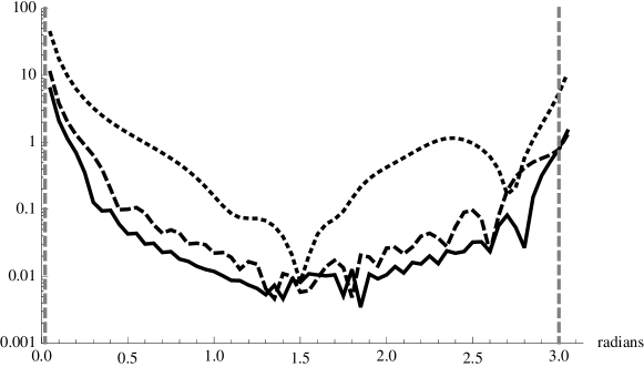
Figure 4: Fractional percentage difference between the values of the $l=0$, $m=0$ overlap reduction function $\Gamma^{L}_{00}(f)$ calculated (i) semi-analytically (i.e., using the analytic expression for $I_{lm}(y,x)$ derived in App. G, and doing the $x$-integration numerically), and (ii) doing the full $(\theta,\phi)$ sky integration numerically using a HEALPix Górski et al. (2005) pixelisation of the sky. The dotted curve is for $y_{1}=10$, $y_{2}=20$; the dashed curve is for $y_{1}=50$, $y_{2}=100$; and the solid curve is for $y_{1}=100$, $y_{2}=200$, where $y_{I}=2\pi fL_{I}/c$ and $L_{I}$ is the distance to pulsar $I$. Note that the percentage difference decreases as $y_{1}$ and $y_{2}$ increase. The vertical dashed grey lines at the left and right-hand edges of the plot correspond to the minimum and maximum angular separation ($0.95$ degrees and 174 degrees, respectively) over all pairs of pulsars in the European Pulsar Timing Array (EPTA).

$l$	$\zeta=0$		$\zeta=\pi$
	Real	Imaginary	Real	Imaginary
$0$	$261$	$117$	$3.31$	$0.254$
$1$	$-445$	$-201$	$-6.78$	$-0.388$
$2$	$561$	$254$	$6.19$	$0.567$
$3$	$-639$	$-290$	$-6.44$	$-0.590$

Table 1: Values of the co-directional ($\zeta=0$) and anti-directional ($\zeta=\pi$) overlap reduction function for a scalar-longitudinal GW background given for $l=0,1,2,3$. The pulsars have $y_{1}=100$ and $y_{2}=200$. The values in the table correspond to $m=0$ modes since all other values of $m$ give zero overlap reduction function values.

III.4 Vector-longitudinal backgrounds

If we ignore the pulsar term, then the response for a vector-longitudinal background, Eq. (39), looks singular at $\cos\theta=-1$. However, due to the factor of $\sin\theta$ in the numerator this is a $1/\sqrt{1+\cos\theta}$ type singularity which is integrable. We can therefore also ignore the pulsar term for these backgrounds and obtain a finite result. The analytic calculation is very similar to that in App. E of Gair et al. (2014) for the standard $(+,\times)$ tensor backgrounds of GR. Details of the calculation are given in App. J. Plots of $\Gamma^{X}_{lm}$ for $l=0,1,2,3$ and $m\geq 0$ are shown in Fig. 5. [$\Gamma^{Y}_{lm}=0$ as a consequence of $R^{Y}_{1}(f,\hat{k})=0$ in the computational frame.]

Figure 5: Plots of $\Gamma^{X}_{lm}$ for $l=0,1,2,3$ as a function of the angle between the two pulsars for an uncorrelated, anisotropic background.

We note that in the limit $\cos\zeta\rightarrow 1$, the $m=0$ overlap reduction functions diverge. This is because in that limit the singularities at $(1+\hat{k}\cdot\hat{u}_{1})=0$ and $(1+\hat{k}\cdot\hat{u}_{2})=0$ coincide and behave like $1/(1+\cos\theta)$ rather than $1/\sqrt{1+\cos\theta}$. Again, this singularity is eliminated if the pulsar terms are included in the integrand and the pulsars are assumed to be at finite distance. Details of that calculation are given in App. J.1.

IV Mapping the background

In Gair et al. (2014) we applied the methodology used to characterise CMB polarisation to describe gravitational-wave backgrounds in general relativity. This involved expanding a transverse tensor GR background in terms of (rank-2) gradients and curls of spherical harmonics, which are closely related to spin-weight $\pm 2$ spherical harmonics. As described in Sec. II.3, we can use a similar decomposition to represent arbitrary backgrounds with alternative polarisation states. As explained earlier, for scalar-transverse and scalar-longitudinal backgrounds, we expand in terms of the ordinary (scalar) spherical harmonics, while for vector-longitudinal backgrounds we must expand in terms of spin-weight $\pm 1$ spherical harmonics.

In the following subsections, we derive analytic expressions for the pulsar response functions $R^{P}_{(lm)}(f)$ defined in Eq. (29), for each mode of a background with each of the different polarisation states, labeled by $P=\{G,C,B,L,V_{G},V_{C}\}$. We calculate the response in the “cosmic” reference frame, where the angular dependence of the gravitational-wave background is to be described. The origin of this frame is at the SSB and a pulsar is located in direction $\hat{u}$, with angular coordinates $(\zeta,\chi)$, i.e.,

$$\hat{u}^{a}=(\sin\zeta\cos\chi,\sin\zeta\sin\chi,\cos\zeta)\,,$$ (51)

and is at a distance $L$ from the SSB. In this frame, we can again make the approximation $\vec{x}\approx\vec{0}$ for the detector locations (i.e., radio receivers on Earth). As was done in Gair et al. (2014), it is simplest to evaluate the response in the cosmic frame by making a change of variables of the integrand of Eq. (29), so that $\hat{u}$ points along the $z$-axis. This corresponds to a rotation defined by the Euler angles $(\alpha,\beta,\gamma)=(\chi,\zeta,0)$. Using the transformation properties of the tensor spherical harmonics $Y^{P}_{(lm)ab}(\hat{k})$ under a rotation, it follows that

$$R^{P}_{(lm)}(f)=Y_{lm}(\hat{u}){\cal R}^{P}_{l}(2\pi fL/c)\,,$$ (52)

where ${\cal R}^{P}_{l}(2\pi fL/c)$ is proportional to the $m=0$ component of the response function calculated in the rotated frame (with the pulsar directed along the $z$-axis):

$${\cal R}^{P}_{l}(2\pi fL/c)\equiv\sqrt{\frac{4\pi}{2l+1}}R^{P}_{(l0)}(f)\big{|}_{\hat{u}=\hat{z}}.$$ (53)

Note that we need only consider the $m=0$ component, since the pulsar response must be axi-symmetric in the rotated frame, while the tensor spherical harmonics we consider are all proportional to $e^{im\phi}$ in this frame. Thus, we see from Eq. (52) that the dependence on the direction to the pulsar is given simply by $Y_{lm}(\hat{u})$, while the distance to the pulsar is responsible for the frequency-dependence of the response function. Finally, using Eq. (29) with $\vec{x}\approx\vec{0}$ and doing the integration over $\phi$, we find

$${\cal R}^{P}_{l}(2\pi fL/c)=2\pi\sqrt{\frac{4\pi}{2l+1}}\int_{-1}^{1}{\rm d}x\>\frac{1}{2}\frac{1}{1+x}Y^{P}_{(l0)zz}(\theta,0)\left(1-e^{-i2\pi fL(1+x)/c}\right)\,,$$ (54)

where $x=\cos\theta$. It is this function that we need to evaluate in the following subsections.

We finish this subsection by noting an important result implicit in Eq. (52) connected to the distinguishability of different background polarisation states. For every polarisation type, the response of a pulsar factorises into a piece that is dependent on pulsar position, which is $Y_{lm}(\hat{u})$ for all polarisation types, and a piece that depends only on the distance to the pulsar. Even if we had infinitely many pulsars distributed across the sky, at any given frequency, the best we could do would be to construct a pulsar response map across the sky and decompose it into (scalar) spherical harmonics. The coefficient of each term would be a sum of the ${\cal R}^{P}_{l}(2\pi fL/c)$’s for all polarisation states, $P$, which at face value means that it would not be possible to disentangle the different polarisation states. However, as we will see below, a scalar-transverse and transverse tensor background can always be distinguished as current PTAs operate in a regime in which the response functions are effectively independent of the pulsar distance, i.e., the pulsar term can be ignored. In that limit, we are only sensitive to modes with $l<2$ of scalar-tensor backgrounds, while transverse tensor backgrounds can only contain modes with $l\geq 2$. The longitudinal modes cannot be distinguished from the transverse modes, however, unless we have several pulsars, at different distances, in each direction on the sky. For the longitudinal modes the finite-distance corrections introduced by the pulsar term are important for typical pulsar distances of current PTAs, which gives an additional handle to identify those modes. Alternatively, if we made some assumption about how the background amplitude was correlated at different frequencies, e.g., that it followed a power law, we would also break this degeneracy as the response of the array to longitudinal modes has a frequency dependence through the same term. Thus, it is in principle possible to disentangle every component of the background for each polarisation state at each frequency, given sufficiently many pulsars at a sufficient variety of distances along each line of sight. In practice, a pulsar timing array containing $N_{p}$ pulsars can only measure $2N_{p}$ real components of the background at any given frequency Gair et al. (2014); Cornish and van Haasteren (2014) and so the resolution of any reconstructed map of the background will be limited by the size of the pulsar timing array. Roughly speaking, to probe an angular scale of the order $1/l_{\rm max}$ we would require $N_{p}=(l_{\rm max}+1)^{2}-4$ pulsars, if we assumed the background was consistent with GR and therefore contained only transverse tensor polarisation modes. If we allow for arbitrary polarisations we would expect to need $N_{p}=3(l_{\rm max}+1)^{2}$ pulsars, since we now have structure down to $l=0$, and we effectively have three different possible polarisation states — transverse (either scalar or tensor, but they are distinguished by the $l$ of the mode), scalar longitudinal or vector longitudinal. A full investigation of what can be measured in practice is beyond the scope of this current work and we leave it for future study.

IV.1 Standard transverse tensor backgrounds

In Gair et al. (2014), the standard transverse tensor modes of GR were expanded in terms of gradient and curl tensor spherical harmonics, and the corresponding response functions were calculated to be

$$R^{G}_{(lm)}(f)\approx 2\pi(-1)^{l}\>{}^{(2)}\!N_{l}Y_{lm}(\hat{u})\,,\quad R^{C}_{(lm)}(f)\approx 0\,,$$ (55)

where ${}^{(2)}\!N_{l}$ is a normalisation constant defined in Eq. (112) of App C, and the $\approx$ signs means that the pulsar term was ignored for this calculation. Extending the analysis given in Gair et al. (2014) to include the pulsar term, we find

$$R^{G}_{(lm)}(f)=Y_{lm}(\hat{u}){\cal R}^{G}_{l}(2\pi fL/c)\,,\quad R^{C}_{(lm)}(f)=0\,,$$ (56)

where

$${\cal R}^{G}_{l}(y)=2\pi\,\frac{{}^{(2)}N_{l}}{4}\int_{-1}^{1}{\rm d}x\>\left[(1-x)(1-x^{2})\left(1-{\rm e}^{-iy(1+x)}\right)\frac{{\rm d}^{2}P_{l}}{{\rm d}x^{2}}\right]\,.$$ (57)

Integrating Eq. (57) by parts twice,

$${\cal R}^{G}_{l}(y)=\pi\,{}^{(2)}\!N_{l}(-i)^{l}e^{-iy}\left[(2-2iy+y^{2})j_{l}(y)-i(6+4iy+y^{2})\frac{{\rm d}j_{l}}{{\rm d}y}-(6iy-y^{2})\frac{{\rm d}^{2}j_{l}}{{\rm d}y^{2}}-iy^{2}\frac{{\rm d}^{3}j_{l}}{{\rm d}y^{3}}\right]\,,$$ (58)

where $j_{l}(y)$ denotes a spherical Bessel function, as defined in App. E, and ${\rm d}j_{l}/{\rm d}y$, ${\rm d}^{2}j_{l}/{\rm d}y^{2}$, and ${\rm d}^{3}j_{l}/{\rm d}y^{3}$ can be simplified using Eqs. (135)–(137). Taking the usual limit that the pulsar is many gravitational-wave wavelengths from the Earth ($y\gg 1$), we find ${\cal R}^{G}_{l}(y)\approx 2\pi(-1)^{l}\>{}^{(2)}\!N_{l}$, which is consistent with Eq. (55), where the response functions were calculated without the pulsar term.

IV.2 Scalar-transverse backgrounds

Repeating the calculation in Gair et al. (2014) for an arbitrary scalar-transverse (breathing mode) background, we find

$$R^{B}_{(lm)}(f)=Y_{lm}(\hat{u}){\cal R}^{B}_{l}(2\pi fL_{/}c)\,,$$ (59)

with

$${\cal R}^{B}_{l}(y) =2\pi\frac{1}{\sqrt{2}}\int_{-1}^{1}{\rm d}x\>\frac{1}{2}(1-x)P_{l}(x)\left(1-{\rm e}^{-i(1+x)y}\right)$$ (60)

$$=2\pi\frac{1}{\sqrt{2}}\left\{\delta_{l0}-\frac{1}{3}\delta_{l1}-(-i)^{l}{\rm e}^{-iy}\left[\left(1-i\frac{l}{y}\right)j_{l}(y)+ij_{l+1}(y)\right]\right\}\,,$$

where we used Eqs. (128), (135) from App. E to get the terms involving the spherical Bessel functions. Since the spherical Bessel functions behave like $1/y$ for large $y$, the terms in square brackets tend to zero as $y\rightarrow\infty$, leading to the approximate expression for the response function

$$R^{B}_{(lm)}(f)\approx 2\pi Y_{lm}(\hat{u})\,\frac{1}{\sqrt{2}}\left[\delta_{l0}-\frac{1}{3}\delta_{l1}\right],$$ (61)

which is valid in the limit where we ignore the pulsar term.

Equation (61) contains a key result of this paper. In the limit that $y\rightarrow\infty$, where the influence of the pulsar term tends to zero, we find that PTAs will completely lack sensitivity to any angular structure beyond $l=1$ in a gravitational-wave background with scalar-transverse polarisation. We can verify this analytic result through numerical map making and recovery. Using

$$h_{B}(f,\hat{k})=\frac{1}{\sqrt{2}}\sum_{l=0}^{\infty}\sum_{m=-l}^{l}a_{lm}^{B}(f)Y_{lm}(\hat{k})\,,$$ (62)

which relates the expansion coefficients $h_{B}(f,\hat{k})$ and $a^{B}_{(lm)}(f)$ in the polarisation and spherical harmonic bases (see Secs. II.2, II.3), we generate a random scalar-transverse (breathing mode) background with angular structure up to and including $l=10$. This injected map is shown in the left panel of Fig. 6. To compute the PTA response to such a background, we generate a random array of $N_{p}=50$ pulsars scattered isotropically across the sky. We work in the polarisation basis rather than the spherical-harmonic basis here, since the PTA response to different angular scales in the GW background is trivial in the latter, and we seek a numerical confirmation of Eq. (60). The PTA response is computed (with a sky resolution set by a given number of pixels $N_{\rm pix}$) using the Earth term component of Eq. (28), by taking the dot product of the array response matrix, $\mathbf{R}$, with the vector of amplitude values at each sky-location, $\mathbf{h}$. The matrix $\mathbf{R}$ has dimensions $(N_{p}\times N_{\rm pix})$, with each element corresponding to the response of a particular pulsar to gravitational waves propagating in a certain direction (denoted by a map pixel), as given by the integrand of Eq. (28). The resulting vector is the signal observed by the full array, $\mathbf{r}=\mathbf{R}\mathbf{h}$. We can invert this in a noiseless map recovery by taking the dot product of the Moore-Penrose pseudoinverse of $\mathbf{R}$ with this observed signal vector. The recovered scalar-transverse sky is shown in the right-hand panel of Fig. 6, where we note a lack of small-scale angular structure. We compute the angular power spectrum of the recovered and injected maps via HEALPix (Górski et al., 2005), which is capable of rapid map decompositions. The results are shown in the left-hand panel of Fig. 7, where we see that despite the injected map having structure up to $l=10$, the recovered map only contains structure up to and including the dipole. This numerical result is a confirmation of the corresponding analytic computation in Eq. (61).

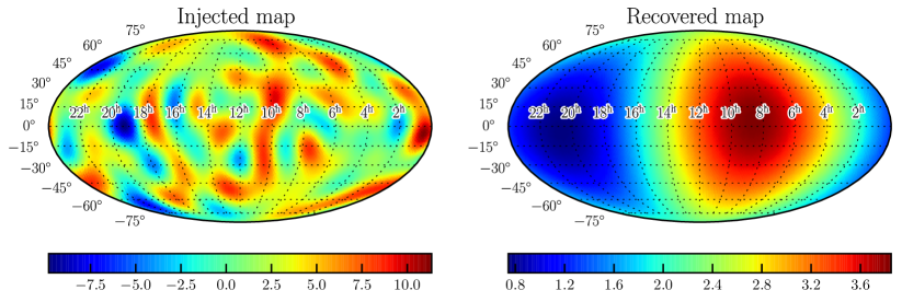
Figure 6: Maps of the real amplitude component of a scalar transverse (breathing mode) background. (Left) a randomly generated scalar-transverse gravitational-wave sky, with structure up to and including $l=10$. (Right) the corresponding recovered sky, computed by first forming the observed signal vector for an array of $N_{p}=50$ pulsars via $\mathbf{r}=\mathbf{R}\mathbf{h}$, where each element of the array response matrix, $\mathbf{R}$, corresponds to the response of a particular pulsar to gravitational waves propagating in a given sky direction. We perform a noiseless map recovery by computing $\mathbf{R}^{+}\mathbf{r}$ (where $\mathbf{R}^{+}$ is the pseudo-inverse of $\mathbf{R}$) which gives the map in the right panel. We note the lack of small-scale angular structure in the recovered map compared to the injected map.

We can also check Eqs. (59) and (60), which imply that the PTA response to a scalar-transverse background will extend beyond the dipole for pulsars at finite distances. We do so again with numerical map making and recovery, by using the full Earth and pulsar term scalar-transverse response function given in Eq. (28). The pulsar term will be highly oscillatory across the sky, so we expect some numerical fluctuations in our results. For this study we inject white Gaussian noise in each pulsar measurement, with an amplitude such that the GW background remains in the strong signal limit. In the right-hand panel of Fig. 7 we see that the PTA has increasing sensitivity to higher multiple moments in the background as $y$ is increased. At $y\sim 5-10$ the PTA is able to recover the full angular structure of the background, but also suffers from noise leakage at higher multipoles, since the non-zero response of the pulsar term at these higher multipoles amplifies noise arising from the pixelation of the sky. The pulsar term response peaks at $l\sim y$, such that for PTAs with $y=15,20$ we see a drop-off in sensitivity at $l\sim 15,20$, even though the response is merely amplifying pixel noise at these multipoles. For $y\gtrsim 20$ the Earth term behaviour is recovered, and we observe a lack of sensitivity to modes beyond dipole. To put these results into context, we recall that $y=2\pi fL/c$ and peak PTA sensitivity to a gravitational-wave background occurs at $f\sim 1/T$ where $T$ is the total observation time. For $T=20$ years, this gives $f\sim 1.6~{}{\rm nHz}$. Thus in order for a PTA to have sensitivity to structure in a scalar-transverse sky beyond dipole, we need $y\lesssim 10$, which corresponds to all pulsars in our array being at a distance of $\lesssim 0.01$ kpc from Earth. Given that most timed millisecond pulsars have distances $\gtrsim 0.2$ kpc, it is unlikely that this extended reach to sensitivity beyond dipole modes will be possible with current arrays.

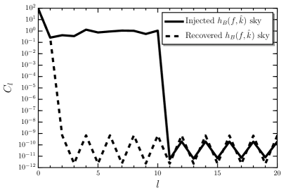
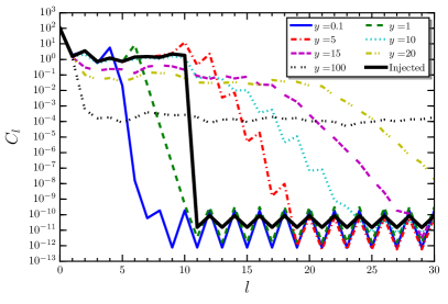
Figure 7: (Left) A comparison of the angular power spectra of the injected scalar-transverse sky map shown in the left-hand panel of Fig. 6, and the PTA-recovered map shown in the right-hand panel of the same figure. We see that PTAs will completely lack sensitivity to angular structure in a scalar-transverse gravitational-wave sky beyond the dipole level. This result is confirmed analytically in Eq. (61). (Right) We use the full Earth and pulsar term response from Eq. (28) to investigate map recovery with finite $y$. The pulsar-term will be highly oscillatory across the sky, so we expect some numerical fluctuations in our results. As $y$ is increased the PTA shows greater sensitivity to higher multipole moments in the GW background. At $y=10$ the PTA is able to recover all modes in the injected map, although the non-zero sensitivity of the pulsar-term response at higher multipoles amplifies noise from the pixelation of the sky. For $y\gtrsim 20$ the Earth term behavior is recovered, and we observe a lack of sensitivity to modes beyond dipole. See text for further details.

Using the mapping response functions $R^{B}_{(lm)}(f)$ calculated above, we can also compute the overlap reduction function for an uncorrelated, anisotropic background, recovering the result given in Sec. III.2. Details of that calculation are given in App. L.

IV.3 Scalar-longitudinal backgrounds

For an arbitrary scalar-longitudinal background we find

$$R^{L}_{(lm)}(f) =Y_{lm}(\hat{u}){\cal R}^{L}_{l}(2\pi fL/c)\,,$$ (63)

where

$${\cal R}^{L}_{l}(y) \equiv 2\pi\int_{-1}^{1}{\rm d}x\>\frac{1}{2}\frac{x^{2}}{1+x}P_{l}(x)\left(1-{\rm e}^{-iy(1+x)}\right)$$ (64)

$$=2\pi\int_{-1}^{1}{\rm d}x\>\frac{1}{2}\left[-1+x+\frac{1}{1+x}\right]P_{l}(x)\left(1-{\rm e}^{-iy(1+x)}\right)$$

$$=2\pi\left\{-\delta_{l0}+\frac{1}{3}\delta_{l1}+(-i)^{l}{\rm e}^{-iy}\left[\left(1-i\frac{l}{y}\right)j_{l}(y)+ij_{l+1}(y)\right]+\frac{1}{2}H_{l}(y)\right\}\,,$$

where $H_{l}(y)$ is defined by Eq. (163) in App. H. Since the spherical Bessel functions behave like $1/y$ for large $y$, the terms in the square brackets above tend to zero as $y\rightarrow\infty$, yielding

$$R^{L}_{(lm)}(f)\approx 2\pi Y_{lm}(\hat{u})\left[-\delta_{l0}+\frac{1}{3}\delta_{l1}+\frac{1}{2}H_{l}(y)\right]\,.$$ (65)

This is valid for $y\gg 1$, but $y$ finite.

IV.4 Vector-longitudinal backgrounds

As discussed in Sec. II.2, we can expand each Fourier component of a vector-longitudinal background in terms of gradient and curl tensor spherical harmonics $Y^{V_{G}}_{(lm)ab}(\hat{k})$, $Y^{V_{C}}_{(lm)ab}(\hat{k})$, which are simply related to the spin-weight $\pm 1$ spherical harmonics defined in App. B. It is convenient to relate this expansion

$$h_{ab}(f,\hat{k})=\sum_{l=1}^{\infty}\sum_{m=-l}^{l}\left[a^{V_{G}}_{(lm)}(f)Y^{V_{G}}_{(lm)ab}(\hat{k})+a^{V_{C}}_{(lm)}(f)Y^{V_{C}}_{(lm)ab}(\hat{k})\right]$$ (66)

to a similar expansion in terms of the polarisation basis:

$$h_{ab}(f,\hat{k})=h_{X}(f,\hat{k})e^{X}_{ab}(\hat{k})+h_{Y}(f,\hat{k})e^{Y}_{ab}(\hat{k})\,.$$ (67)

The relationship is

$$h_{X}(f,\hat{k})\pm ih_{Y}(f,\hat{k})=\mp\frac{1}{\sqrt{2}}\sum_{lm}\left(a^{V_{G}}_{(lm)}(f)\pm ia^{V_{C}}_{(lm)}(f)\right){}_{\pm 1}Y_{lm}(\hat{k})\,,$$ (68)

or, equivalently,

$$h_{X}(f,\hat{k}) =\frac{1}{2\sqrt{2}}\sum_{lm}\left[a^{V_{G}}_{(lm)}(f)\left({}_{-1}Y_{lm}(\hat{k})-{}_{1}Y_{lm}(\hat{k})\right)-ia^{V_{C}}_{(lm)}(f)\left({}_{-1}Y_{lm}(\hat{k})+{}_{1}Y_{lm}(\hat{k})\right)\right],$$ (69)

$$h_{Y}(f,\hat{k}) =\frac{1}{2\sqrt{2}}\sum_{lm}\left[a^{V_{C}}_{(lm)}(f)\left({}_{-1}Y_{lm}(\hat{k})-{}_{1}Y_{lm}(\hat{k})\right)+ia^{V_{G}}_{(lm)}(f)\left({}_{-1}Y_{lm}(\hat{k})+{}_{1}Y_{lm}(\hat{k})\right)\right]\,,$$

where ${}_{\pm 1}\!Y_{lm}(\hat{k})$ are the spin-weight $\pm 1$ spherical harmonics defined in App. A.

The expressions for the grad and curl response functions for an arbitrary vector-longitudinal background can be calculated using the same methods as in the preceding subsections. We find

$$R^{V_{G}}_{I(lm)}(f)=Y_{lm}(\hat{u}_{I}){\cal R}^{V_{G}}_{l}(2\pi fL_{I}/c)\,,\qquad R^{V_{C}}_{I(lm)}(f)=0\,,$$ (70)

where

$${\cal R}^{V_{G}}_{l}(y) =\pi\,{}^{(1)}\!N_{l}\int_{-1}^{1}{\rm d}x\>\left[x(1-x)\left(1-{\rm e}^{-iy(1+x)}\right)\frac{{\rm d}P_{l}}{{\rm d}x}\right]\,.$$ (71)

Thus, the response to vector curl modes is identically zero for pulsar timing arrays, as is the case for tensor curl modes, as shown in Gair et al. (2014). Evaluating the integral in Eq. (71) by parts we find

$$R^{V_{G}}_{l}(y) =\pi\,{}^{(1)}\!N_{l}\left[-2\delta_{l0}+\frac{4}{3}\delta_{l1}+(-1)^{l}{\rm e}^{-iy}\int_{-1}^{1}{\rm d}x\>(1+(2+iy)x+iyx^{2}){\rm e}^{iyx}P_{l}(x)\right]$$ (72)

$$=\pi\,{}^{(1)}\!N_{l}\left\{\frac{4}{3}\delta_{l1}+2(-i)^{l}{\rm e}^{-iy}\left[\left(1-\frac{il}{y}\right)(l+1)j_{l}(y)-(y-i(2l+3))j_{l+1}(y)-iyj_{l+2}(y)\right]\right\},$$ (73)

where we have dropped the $\delta_{l0}$ term since for spin-weight $\pm 1$ harmonics we have $l\geq 1$. Taking the usual limit that the pulsar is many gravitational-wave wavelengths from the Earth, $y\gg 1$, and using the asymptotic result

$$j_{l}(y)\approx\frac{1}{y}\sin\left(y-\frac{l\pi}{2}\right)+O\left(\frac{1}{y^{\frac{3}{2}}}\right)\,,\quad{\rm for\ }y\gg 1,$$ (74)

we find

$$R^{V_{G}}_{lm}(f)\approx 2\pi Y_{lm}(\hat{u})\left[\frac{2}{3}\delta_{l1}+(-1)^{l}\,{}^{(1)}\!N_{l}\right]\,.$$ (75)

As expected, this agrees with the result obtained by evaluating the integral in Eq. (71) without the pulsar term, i.e., making the replacement $\{1-\exp[-iy(1+x)]\}\rightarrow 1$.

IV.5 Overlap reduction function for statistically isotropic backgrounds

For a statistically isotropic, unpolarized and parity-invariant background (see, for example, Eqs. (52)–(54) of Gair et al. (2014))

$$\Gamma(f)=\sum_{l}C_{l}\Gamma_{l}(f),$$ (76)

where

$$\Gamma_{l}(f)=\sum_{m=-l}^{l}\sum_{P}R_{1(lm)}^{P}(f)R_{2(lm)}^{P*}(f).$$ (77)

Here $\sum_{P}$ is a sum over the polarization states for a particular type of background (e.g., $P=\{V_{G},V_{C}\}$ or $P=\{G,C\}$ for vector-longitudinal or transverse tensor backgrounds). Using the results of the previous subsections, we have in the limit $y_{1}\gg 1$, $y_{2}\gg 1$ (where $y_{I}=2\pi fL_{I}/c$ as before):

Transverse tensor modes ($l\geq 2$):

$$\Gamma^{T}_{l}(f)\approx\pi(2l+1)(N^{T}_{l})^{2}P_{l}(\cos\zeta)\,,$$ (78)

which was found in Gair et al. (2014).
Scalar-transverse mode ($l\geq 0$):

$$\Gamma^{B}_{l}(f)\approx\pi(2l+1)\frac{1}{2}\left[\delta_{l0}+\frac{1}{9}\delta_{l1}\right]\,P_{l}(\cos\zeta)\,.$$ (79)

Scalar-longitudinal mode ($l\geq 0$):

$$\Gamma^{L}_{l}(f)\approx\pi(2l+1)\left\{\delta_{l0}\left[1-\frac{1}{2}\left(H_{0}(y_{1})+H_{0}^{*}(y_{2})\right)\right]+\delta_{l1}\left[\frac{1}{9}+\frac{1}{6}\left(H_{1}(y_{1})+H_{1}^{*}(y_{2})\right)\right]+\frac{1}{4}H_{l}(y_{1})H_{l}^{*}(y_{2})\right\}P_{l}(\cos\zeta)\,.$$ (80)

Vector-longitudinal modes ($l\geq 1$):

$$\Gamma^{V}_{l}(f)\approx\pi(2l+1)({}^{(1)}\!N_{l})^{2}\left[-\frac{8}{9}\delta_{l1}+1\right]P_{l}(\cos\zeta)\,.$$ (81)

Note that only the scalar-longitudinal overlap reduction functions $\Gamma^{L}_{l}(f)$ are actually frequency-dependent in the large $y$ limit, via their dependence on $H_{l}(y_{I})$. The other overlap reduction functions depend only on the angular separation $\zeta$ between the pair of pulsars.

As shown in Gair et al. (2014), an isotropic, unpolarized and uncorrelated background has $C_{l}=1$ for all $l$. In Fig. 8 we plot approximations to $\Gamma^{B}$, $\Gamma^{L}$, $\Gamma^{V}$, and $\Gamma^{T}$ corresponding to different values of $l_{\rm max}$ in the summation of Eq.(̃76), taking $C_{l}=1$ for all $l$ up to $l_{\rm max}$. (Recall that for the vector overlap reduction function, the summation starts at $l=1$, while for the tensor overlap reduction function, it starts at $l=2$.) These finite $l_{\rm max}$ expressions are compared to the $l=0$, $m=0$ components of the overlap reduction functions calculated in Sec. III and plotted in Figs. 1, 2, 3, 5. The normalization is different than in those figures, since the $l=0$, $m=0$ components need to be multiplied by $\sqrt{4\pi}/2$ in order to obtain the isotropic overlap reduction function. (The factor of $\sqrt{4\pi}$ comes from $Y_{00}(\hat{k})=1/\sqrt{4\pi}$; the factor of $1/2$ is needed to get agreement between Eq. (43) and Eq. (32) of Gair et al. (2014) for isotropic, unpolarized backgrounds.)

Figure 8 confirms what was found for the transverse tensor modes in Gair et al. (2014), namely that a good approximation to the full overlap reduction function can be obtained by including only a relatively small number of modes in the sum. The maximum $l$ required in the sum is approximately $1,4,10$ and $20$ for the scalar-transverse, transverse tensor, vector-longitudinal and scalar-longitudinal backgrounds respectively.

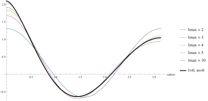
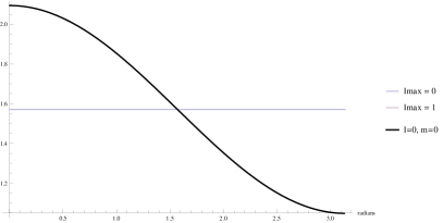
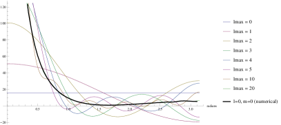
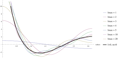
Figure 8: Approximations to the overlap reduction functions for an isotropic, unpolarized and uncorrelated stochastic background, plotted as a function of the angle between a pair of pulsars. The approximations are obtained by summing products of the response functions over $l$ for different values of $l_{\rm max}$. Panel (a): transverse tensor background; Panel (b): scalar-transverse (breathing) background; panel (c): scalar-longitudinal background; panel (d): vector-longitudinal background. We are working in the large $y$ limit for all of these cases. For the scalar-longitudinal background, we have taken $y_{1}=100$ and $y_{2}=200$. The thick black line in each plot is the “full” expression for the overlap reduction function, corresponding to the limit $l_{\rm max}\rightarrow\infty$. (These limiting expressions equal $\sqrt{4\pi}/2$ times the $l=0$, $m=0$ component of the overlap reduction functions calculated in Sec. III.) For the scalar-longitudinal case, the full expression was calculated numerically.

V Conclusion

In this paper we have investigated the overlap reduction functions and response functions of PTAs for non-GR polarisations of gravitational waves. The overlap reduction function describes the sensitivity of a pair of pulsars to a gravitational-wave background in a cross-correlation analysis. The cross-correlation signature traced out by the overlap reduction function from an entire array of precisely-timed millisecond pulsars will aid in isolating any gravitational-wave signal from other stochastic processes which may have similar spectral properties. Hence, current searches for stochastic gravitational-wave backgrounds rely on models of the overlap reduction function as the smoking-gun signature of a signal. For an isotropic stochastic background in GR, the overlap reduction function is known as the Hellings and Downs curve, and depends only on the angular separation between pulsars in the array. The overlap reduction functions for arbitrary anisotropic stochastic backgrounds in GR were investigated in Gair et al. (2014); Mingarelli et al. (2013), where it was shown that these functions are now dependent on the positions of each pulsar relative to the distribution of gravitational-wave power on the sky.

The gravitational wave polarisation has a strong influence on the overlap reduction function through the form of the pulsar response functions. Chamberlin and Siemens (2012) studied the form of the overlap reduction functions for isotropic backgrounds of gravitational waves for scalar-transverse, scalar-longitudinal, and vector-longitudinal polarisation modes. In this paper, we have extended that analysis to find analytic expressions for the overlap reduction functions for anisotropic non-GR backgrounds. A key result of this work is that PTAs will completely lack sensitivity to structure beyond quadrupole in the power of a scalar-transverse background. This result holds regardless of the number of pulsars, timing-precision, or observational schedules—it is a property of the geometric sensitivity of PTAs to gravitational-wave signals of scalar-transverse polarisation. Additionally, we have found analytic expressions for the overlap reduction functions for arbitrary anisotropic vector-longitudinal backgrounds. We also derived a semi-analytic expression for the overlap reduction functions of anisotropic scalar-longitudinal backgrounds, in which case a consideration of the pulsar-term is crucial to avoid divergences.

In the second half of this paper, we extended the formalism of our previous work in Gair et al. (2014), where the Fourier amplitudes in a plane-wave expansion of the GR metric perturbation were decomposed with respect to a basis of gradient and curl spherical harmonics, which are related to spin-weight $\pm 2$ spherical harmonics. By determining the components of the background in such a decomposition it is possible to construct a map of both the amplitude and the phase of the gravitational wave background across the sky, rather than simply reconstructing the power distribution. The decomposition in terms of spin-weight $\pm 2$ spherical harmonics is made possible by the transverse-traceless nature of the GR gravitational-wave metric perturbations. Here we have appealed to the structure of the gravitational-wave metric perturbations for non-GR polarisations to perform the same procedure—the Fourier amplitudes of scalar modes can be expanded in terms of ordinary spin-weight $0$ spherical harmonics, while the vector mode amplitudes can be expanded in terms of a spin-weight $\pm 1$ spherical harmonic basis. In so doing, we found that PTAs lack sensitivity to structure in the polarisation amplitude of a scalar-transverse background beyond dipole anisotropy, which can be used to explain the lack of sensitivity to power anisotropies beyond quadrupole. This result was verified through numerical map making and recovery, where we found some sensitivity to modes beyond dipole when $y=2\pi fL/c$ was very small, but this would require all pulsars to lie within a distance of $0.01$ kpc from Earth. We also found that PTAs will lack sensitivity to vector curl modes for a vector-longitudinal background, which is analogous to the finding in Gair et al. (2014) that PTAs are insensitive to the tensor curl modes of gravitational-wave backgrounds in GR.

This paper provides several ready-to-use expressions for overlap reduction functions for non-GR stochastic backgrounds with arbitrary anisotropy. These expressions can be trivially plugged into any current or planned PTA stochastic background search pipeline to obtain limits on the strain amplitude of a non-GR gravitational-wave sky. We also provide several ready-to-use expressions for the response functions of a single pulsar to anisotropies in a non-GR gravitational-wave background. The implications of this are that we can use an array of pulsars to perform a Bayesian or frequentist search for the angular dependence of the Fourier modes of a plane-wave expansion of the gravitational-wave metric perturbations, and in so doing produce maps of the polarisation content of the sky that include phase information rather than simply map the distribution of power.

The results in this paper also indicate what is possible to measure in principle with a sufficiently extensive pulsar timing array. The dependence of the response on the pulsar location on the sky is proportional to $Y_{lm}(\hat{u})$, where $\hat{u}$ is the direction to the pulsar, for all polarisation types. By decomposing the pulsar response map, at a particular frequency, into regular (scalar) spherical harmonics, the coefficients of each $Y_{lm}(\hat{u})$ mode of the response map can be determined, but these coefficients will be a sum of the contributions from each of the polarisation types. Scalar-transverse and transverse tensor backgrounds can be distinguished because PTAs typically operate in a regime in which the pulsar term is negligible and so the response is independent of the distance to the pulsar. In that regime, PTAs are only sensitive to modes of the scalar-transverse background with $l<2$, while transverse tensor backgrounds can only contain modes with $l\geq 2$. However, longitudinal backgrounds can only be distinguished from transverse backgrounds if there are multiple pulsars along a given line of sight, or if there is a known correlation (e.g., a power law) between the background amplitudes at different frequencies. In either of these scenarios, we can exploit the dependence of the pulsar term on $2\pi fL/c$, which is much more significant for the longitudinal modes of the background. Thus, in the limit of infinitely many pulsars distributed across the sky at a range of distances, we would expect to be able to measure the entire content of the background in each polarisation state and at each frequency. In practice, of course, a pulsar timing array of $N_{p}$ pulsars can only measure $2N_{p}$ real components of the background Gair et al. (2014); Cornish and van Haasteren (2014), and so the resolution of any map that we produce will be limited by the number of pulsars in the array. Roughly speaking, to produce a map of the gravitational wave sky in all polarisation states to an angular resolution of $1/l_{\rm max}$ would require $N_{p}=3(l_{\rm max}+1)^{2}$ pulsars, but this should be explored more carefully in the future.

For a further discussion of the prospects of this type of mapping analysis, see Gair et al. (2014); Cornish and van Haasteren (2014). We plan to apply the results of this paper to the analysis of real data, to map the amplitude and phase content of non-GR gravitational-wave backgrounds influencing the arrival times of millisecond pulsars. This will allow us to place constraints on beyond-GR polarisations of nanohertz gravitational waves.

Appendix A Spin-weighted spherical harmonics

This appendix summarizes some useful relations involving spin-weighted and ordinary spherical harmonics, ${}_{s}Y_{lm}(\hat{k})$ and $Y_{lm}(\hat{k})$. For more details, see e.g., Goldberg et al. (1967) and del Castillo (2003). Note that we use a slightly different normalization convention than in Goldberg et al. (1967). Namely, we put the Condon-Shortley factor $(-1)^{m}$ in the definition of the associated Legendre functions $P_{l}^{m}(x)$, and thus do not explicitly include it in the definition of the spherical harmonics. Also, for our analysis, we can restrict attention to spin-weighted spherical harmonics having integral spin weight $s$, even though spin-weighted spherical harmonics with half-integral spin weight do exist.

Ordinary spherical harmonics:

$$Y_{lm}(\hat{k})=Y_{lm}(\theta,\phi)=N_{l}^{m}P_{l}^{m}(\cos\theta)e^{im\phi}\,,\quad{\rm where}\ N_{l}^{m}=\sqrt{\frac{2l+1}{4\pi}\frac{(l-m)!}{(l+m)!}}.$$ (82)

Relation of spin-weighted spherical harmonics to ordinary spherical harmonics:

$${}_{s}Y_{lm}(\theta,\phi) =\sqrt{\frac{(l-s)!}{(l+s)!}}\,\check{\partial}^{s}Y_{lm}(\theta,\phi)\quad{\rm for}\quad 0\leq s\leq l\,,$$ (83)

$${}_{s}Y_{lm}(\theta,\phi) =\sqrt{\frac{(l+s)!}{(l-s)!}}\,(-1)^{s}\overline{\check{\partial}}{}^{-s}Y_{lm}(\theta,\phi)\quad{\rm for}\quad-l\leq s\leq 0\,,$$

where

$$\check{\partial}\eta =-(\sin\theta)^{s}\left[\frac{\partial}{\partial\theta}+i\csc\theta\frac{\partial}{\partial\phi}\right](\sin\theta)^{-s}\eta\,,$$ (84)

$$\overline{\check{\partial}}\eta =-(\sin\theta)^{-s}\left[\frac{\partial}{\partial\theta}-i\csc\theta\frac{\partial}{\partial\phi}\right](\sin\theta)^{s}\eta\,,$$

and $\eta=\eta(\theta,\phi)$ is a spin-$s$ scalar field.

Series representation:

$${}_{s}Y_{lm}(\theta,\phi)=(-1)^{m}\left[\frac{(l+m)!(l-m)!}{(l+s)!(l-s)!}\frac{2l+1}{4\pi}\right]^{1/2}(\sin\theta/2)^{2l}\sum_{k=0}^{l-s}\binom{l-s}{k}\binom{l+s}{k+s-m}(-1)^{l-k-s}e^{im\phi}(\cot\theta/2)^{2k+s-m}.$$ (85)

Complex conjugate:

$${}_{s}Y_{lm}^{*}(\theta,\phi)=(-1)^{m+s}\,{}_{-s}Y_{l,-m}(\theta,\phi).$$ (86)

Relation to Wigner rotation matrices:

$$D^{l}{}_{m^{\prime}m}(\phi,\theta,\psi)=(-1)^{m^{\prime}}\sqrt{\frac{4\pi}{2l+1}}\,{}_{m}Y_{l,-m^{\prime}}(\theta,\phi)e^{-im\psi},$$ (87)

or

$$\left[D^{l}{}_{m^{\prime}m}(\phi,\theta,\psi)\right]^{*}=(-1)^{m}\sqrt{\frac{4\pi}{2l+1}}\,{}_{-m}Y_{l,m^{\prime}}(\theta,\phi)e^{im\psi}.$$ (88)

Parity transformation:

$${}_{s}Y_{lm}(\pi-\theta,\phi+\pi)=(-1)^{l}\,{}_{-s}Y_{lm}(\theta,\phi).$$ (89)

Orthonormality (for fixed $s$):

$$\int_{S^{2}}{\rm d}^{2}\Omega_{\hat{k}}\>{}_{s}Y_{lm}(\hat{k})\,{}_{s}Y_{l^{\prime}m^{\prime}}^{*}(\hat{k})\equiv\int_{0}^{2\pi}{\rm d}\phi\int_{0}^{\pi}\sin\theta\,{\rm d}\theta\>{}_{s}Y_{lm}(\theta,\phi)\,{}_{s}Y_{l^{\prime}m^{\prime}}^{*}(\theta,\phi)=\delta_{ll^{\prime}}\delta_{mm^{\prime}}.$$ (90)

Addition theorem for spin-weighted spherical harmonics:

$$\sum_{m=-l}^{l}{}_{s}Y_{lm}(\theta_{1},\phi_{1})\,{}_{s^{\prime}}Y_{lm}^{*}(\theta_{2},\phi_{2})=(-1)^{-s^{\prime}}\sqrt{\frac{2l+1}{4\pi}}\,{}_{-s^{\prime}}Y_{ls}(\theta_{3},\phi_{3})e^{is^{\prime}\chi_{3}},$$ (91)

where

$$\cos\theta_{3}=\cos\theta_{1}\cos\theta_{2}+\sin\theta_{1}\sin\theta_{2}\cos(\phi_{2}-\phi_{1}),$$ (92)

and

$$e^{-i(\phi_{3}+\chi_{3})/2} =\frac{\cos\frac{1}{2}(\phi_{2}-\phi_{1})\cos\frac{1}{2}(\theta_{2}-\theta_{1})-i\sin\frac{1}{2}(\phi_{2}-\phi_{1})\cos\frac{1}{2}(\theta_{1}+\theta_{2})}{\sqrt{\cos^{2}\frac{1}{2}(\phi_{2}-\phi_{1})\cos^{2}\frac{1}{2}(\theta_{2}-\theta_{1})+\sin^{2}\frac{1}{2}(\phi_{2}-\phi_{1})\cos^{2}\frac{1}{2}(\theta_{1}+\theta_{2})}},$$ (93)

$$e^{i(\phi_{3}-\chi_{3})/2} =\frac{\cos\frac{1}{2}(\phi_{2}-\phi_{1})\sin\frac{1}{2}(\theta_{2}-\theta_{1})+i\sin\frac{1}{2}(\phi_{2}-\phi_{1})\sin\frac{1}{2}(\theta_{1}+\theta_{2})}{\sqrt{\cos^{2}\frac{1}{2}(\phi_{2}-\phi_{1})\sin^{2}\frac{1}{2}(\theta_{2}-\theta_{1})+\sin^{2}\frac{1}{2}(\phi_{2}-\phi_{1})\sin^{2}\frac{1}{2}(\theta_{1}+\theta_{2})}}.$$

Addition theorem for ordinary spherical harmonics:

$$\sum_{m=-l}^{l}Y_{lm}(\hat{k}_{1})Y_{lm}^{*}(\hat{k}_{2})=\frac{2l+1}{4\pi}\,P_{l}(\hat{k}_{1}\cdot\hat{k}_{2}).$$ (94)

Integral of a product of spin-weighted spherical harmonics:

$$\int_{S^{2}}{\rm d}^{2}\Omega_{\hat{k}}\>{}_{s_{1}}Y_{l_{1}m_{1}}(\hat{k})\,{}_{s_{2}}Y_{l_{2}m_{3}}(\hat{k})\,{}_{s_{3}}Y_{l_{3}m_{3}}(\hat{k})\,=\sqrt{\frac{(2l_{1}+1)(2l_{2}+1)(2l_{3}+1)}{4\pi}}\left(\begin{array}[]{ccc}l_{1}&l_{2}&l_{3}\\ m_{1}&m_{2}&m_{3}\end{array}\right)\left(\begin{array}[]{ccc}l_{1}&l_{2}&l_{3}\\ -s_{1}&-s_{2}&-s_{3}\end{array}\right),$$ (95)

where $\left(\begin{array}[]{ccc}l_{1}&l_{2}&l_{3}\\ m_{1}&m_{2}&m_{3}\end{array}\right)$ is a Wigner 3-$j$ symbol, which can be written as

$$\left(\begin{array}[]{ccc}l&l^{\prime}&L\\ m&m^{\prime}&M\end{array}\right) = \sqrt{\frac{(l+l^{\prime}-L)!(l-l^{\prime}+L)!(-l+l^{\prime}+L)!(l+m)!(l-m)!(l^{\prime}+m^{\prime})!(l^{\prime}-m^{\prime})!(L+M)!(L-M)!}{(l+l^{\prime}+L+1)!}}\times$$ (99)

$$\hskip 28.45274pt\times\sum_{z\in\mathbb{Z}}\frac{(-1)^{z+l+l^{\prime}-M}}{z!(l+l^{\prime}-L-z)!(l-m-z)!(l^{\prime}+m^{\prime}-z)!(L-l^{\prime}+m+z)!(L-l-m^{\prime}+z)!}.$$

See, for example, Wigner (1959), Messiah (1962), Landau and Lifshitz (1977) and references therein. Note that although this sum is over all integers it contains only a finite number of non-zero terms since the factorial of a negative number is defined to be infinite.

Appendix B Gradient and curl rank-1 (vector) spherical harmonics

The gradient and curl rank-1 (vector) spherical harmonics are defined for $l\geq 1$ by

$$Y^{G}_{(lm)a} \equiv\frac{1}{2}{}^{(1)}\!N_{l}\partial_{a}Y_{lm}=\frac{1}{2}{}^{(1)}\!N_{l}\left(\frac{\partial Y_{lm}}{\partial\theta}\,\hat{\theta}_{a}+\frac{1}{\sin\theta}\frac{\partial Y_{lm}}{\partial\phi}\,\hat{\phi}_{a}\right),$$ (100)

$$Y^{C}_{(lm)a} \equiv\frac{1}{2}{}^{(1)}\!N_{l}(\partial_{b}Y_{lm})\epsilon^{b}{}_{a}=\frac{1}{2}{}^{(1)}\!N_{l}\left(-\frac{1}{\sin\theta}\frac{\partial Y_{lm}}{\partial\phi}\,\hat{\theta}_{a}+\frac{\partial Y_{lm}}{\partial\theta}\,\hat{\phi}_{a}\right),$$

where $\hat{\theta}$ and $\hat{\phi}$ are the standard unit vectors tangent to the 2-sphere

$$\hat{\theta} =\cos\theta\cos\phi\,\hat{x}+\cos\theta\sin\phi\,\hat{y}-\sin\theta\,\hat{z}\,,$$ (101)

$$\hat{\phi} =-\sin\phi\,\hat{x}+\cos\phi\,\hat{y}\,,$$

${}^{(1)}N_{l}$ is a normalisation constant

$${}^{(1)}N_{l}=\sqrt{\frac{2(l-1)!}{(l+1)!}}\,,$$ (102)

and $\epsilon_{ab}$ is the Levi-Civita anti-symmetric tensor

$$\epsilon_{ab}=\sqrt{g}\left(\begin{array}[]{cc}0&1\\ -1&0\end{array}\right)\,,\qquad g\equiv{\rm det}(g_{ab})\,.$$ (103)

Following standard practice, we use the metric tensor on the 2-sphere $g_{ab}$ and its inverse $g^{ab}$ to “lower” and “raise” tensor indices—e.g., $\epsilon^{c}{}_{b}\equiv g^{ca}\epsilon_{ab}$. In standard spherical coordinates $(\theta,\phi)$,

$$g_{ab}=\left(\begin{array}[]{cc}1&0\\ 0&\sin^{2}\theta\\ \end{array}\right)\,,\qquad\sqrt{g}=\sin\theta\,.$$ (104)

The grad and curl spherical harmonics are related to the spin-weight $\pm 1$ spherical harmonics

$${}_{\pm 1}Y_{lm}(\hat{k}) =\sqrt{\frac{(l-1)!}{(l+1)!}}\frac{N_{l}^{m}}{\sqrt{1-x^{2}}}\left(\pm(1-x^{2})\frac{{\rm d}P_{l}^{m}}{{\rm d}x}+mP_{l}^{m}(x)\right){\rm e}^{im\phi}\,,\quad{\rm where}\ x=\cos\theta$$ (105)

via

$$Y^{G}_{(lm)a}(\hat{k})\pm iY^{C}_{(lm)a}(\hat{k})=\pm\frac{1}{\sqrt{2}}(\hat{\theta}_{a}\pm i\hat{\phi}_{a})\,{}_{\mp 1}Y_{lm}(\hat{k})$$ (106)

or, equivalently,

$$Y^{G}_{(lm)a}(\hat{k}) =\frac{1}{2\sqrt{2}}\left[\left({}_{-1}Y_{lm}(\hat{k})-{}_{1}Y_{lm}(\hat{k})\right)\hat{\theta}_{a}+i\left({}_{-1}Y_{lm}(\hat{k})+{}_{1}Y_{lm}(\hat{k})\right)\hat{\phi}_{a}\right],$$ (107)

$$Y^{C}_{(lm)a}(\hat{k}) =\frac{1}{2\sqrt{2}}\left[\left({}_{-1}Y_{lm}(\hat{k})-{}_{1}Y_{lm}(\hat{k})\right)\hat{\phi}_{a}-i\left({}_{-1}Y_{lm}(\hat{k})+{}_{1}Y_{lm}(\hat{k})\right)\hat{\theta}_{a}\right].$$

For decompositions of vector-longitudinal backgrounds, as discussed in the main text, it will be convenient to construct rank-2 tensor fields

$$Y^{V_{G}}_{(lm)ab} =Y^{G}_{(lm)a}\hat{k}_{b}+Y^{G}_{(lm)b}\hat{k}_{a}\,,$$ (108)

$$Y^{V_{C}}_{(lm)ab} =Y^{C}_{(lm)a}\hat{k}_{b}+Y^{C}_{(lm)b}\hat{k}_{a}\,,$$

where $\hat{k}$ is the unit radial vector orthogonal to the surface of the 2-sphere:

$$\hat{k}=\sin\theta\cos\phi\,\hat{x}+\sin\theta\sin\phi\,\hat{y}+\cos\theta\,\hat{z}\,.$$ (109)

These fields satisfy the following orthonormality relations

$$\int_{S^{2}}{\rm d}^{2}\Omega_{\hat{k}}\>Y^{V_{G}}_{(lm)ab}(\hat{k})Y^{V_{G}}_{(l^{\prime}m^{\prime})}{}^{ab\,*}(\hat{k}) =\delta_{ll^{\prime}}\delta_{mm^{\prime}}\,,$$ (110)

$$\int_{S^{2}}{\rm d}^{2}\Omega_{\hat{k}}\>Y^{V_{C}}_{(lm)ab}(\hat{k})Y^{V_{C}}_{(l^{\prime}m^{\prime})}{}^{ab\,*}(\hat{k}) =\delta_{ll^{\prime}}\delta_{mm^{\prime}}\,,$$

$$\int_{S^{2}}{\rm d}^{2}\Omega_{\hat{k}}\>Y^{V_{G}}_{(lm)ab}(\hat{k})Y^{V_{C}}_{(l^{\prime}m^{\prime})}{}^{ab\,*}(\hat{k}) =0\,.$$

Appendix C Gradient and curl rank-2 (tensor) spherical harmonics

The gradient and curl rank-2 (tensor) spherical harmonics are defined for $l\geq 2$ by:

$$Y^{G}_{(lm)ab} =N_{l}\left(Y_{(lm);ab}-\frac{1}{2}g_{ab}Y_{(lm);c}{}^{c}\right)\,,$$ (111)

$$Y^{C}_{(lm)ab} =\frac{N_{l}}{2}\left(Y_{(lm);ac}\epsilon^{c}{}_{b}+Y_{(lm);bc}\epsilon^{c}{}_{a}\right)\,,$$

where a semicolon denotes covariant derivative on the 2-sphere, and ${}^{(2)}N_{l}$ is a normalisation constant

$${}^{(2)}N_{l}=\sqrt{\frac{2(l-2)!}{(l+2)!}}\,.$$ (112)

Using the standard polarisation tensors on the 2-sphere:

$$e^{+}_{ab}(\hat{k}) =\hat{\theta}_{a}\hat{\theta}_{b}-\hat{\phi}_{a}\hat{\phi}_{b}\,,$$ (113)

$$e^{\times}_{ab}(\hat{k}) =\hat{\theta}_{a}\hat{\phi}_{b}+\hat{\phi}_{a}\hat{\theta}_{b}\,,$$

where $\hat{\theta}$, $\hat{\phi}$ are given by Eq. (101), we have Hu and White (1997):

$$Y^{G}_{(lm)ab}(\hat{k}) =\frac{{}^{(2)}N_{l}}{2}\left[W_{(lm)}(\hat{k})e_{ab}^{+}(\hat{k})+X_{(lm)}(\hat{k})e_{ab}^{\times}(\hat{k})\right]\,,$$ (114)

$$Y^{C}_{(lm)ab}(\hat{k}) =\frac{{}^{(2)}N_{l}}{2}\left[W_{(lm)}(\hat{k})e_{ab}^{\times}(\hat{k})-X_{(lm)}(\hat{k})e_{ab}^{+}(\hat{k})\right]\,,$$

where

$$W_{(lm)}(\hat{k}) =\left(\frac{\partial^{2}}{\partial\theta^{2}}-\cot\theta\frac{\partial}{\partial\theta}+\frac{m^{2}}{\sin^{2}\theta}\right)Y_{lm}(\hat{k})=\left(2\frac{\partial^{2}}{\partial\theta^{2}}+l(l+1)\right)Y_{lm}(\hat{k})\,,$$ (115)

$$X_{(lm)}(\hat{k}) =\frac{2im}{\sin\theta}\left(\frac{\partial}{\partial\theta}-\cot\theta\right)Y_{lm}(\hat{k})\,.$$

These functions enter the expression for the spin-weight $\pm 2$ spherical harmonics Newman and Penrose (1966); Goldberg et al. (1967):

$${}_{\pm 2}Y_{lm}(\hat{k})=\frac{{}^{(2)}N_{l}}{\sqrt{2}}\left[W_{(lm)}(\hat{k})\pm iX_{(lm)}(\hat{k})\right]\,,$$ (116)

which are related to the grad and curl spherical harmonics via

$$Y^{G}_{(lm)ab}(\hat{k})\pm iY^{C}_{(lm)ab}(\hat{k}) =\frac{1}{\sqrt{2}}\left(e_{ab}^{+}(\hat{k})\pm ie_{ab}^{\times}(\hat{k})\right)\,{}_{\mp 2}Y_{lm}(\hat{k})\,.$$ (117)

Note that the grad and curl spherical harmonics satisfy the orthonormality relations

$$\int_{S^{2}}{\rm d}^{2}\Omega_{\hat{k}}\>Y^{G}_{(lm)ab}(\hat{k})Y^{G}_{(l^{\prime}m^{\prime})}{}^{ab\,*}(\hat{k}) =\delta_{ll^{\prime}}\delta_{mm^{\prime}}\,,$$ (118)

$$\int_{S^{2}}{\rm d}^{2}\Omega_{\hat{k}}\>Y^{C}_{(lm)ab}(\hat{k})Y^{C}_{(l^{\prime}m^{\prime})}{}^{ab\,*}(\hat{k}) =\delta_{ll^{\prime}}\delta_{mm^{\prime}}\,,$$

$$\int_{S^{2}}{\rm d}^{2}\Omega_{\hat{k}}\>Y^{G}_{(lm)ab}(\hat{k})Y^{C}_{(l^{\prime}m^{\prime})}{}^{ab\,*}(\hat{k}) =0\,.$$

Appendix D Legendre polynomials and associated Legendre functions

The following is a list of some useful identities involving Legendre polynomials $P_{l}(x)$ and associated Legendre functions $P_{l}^{m}(x)$. For additional properties see e.g., Abramowitz and Stegun (1972).

Differential equation:

$$(1-x^{2})\frac{{\rm d}^{2}}{{\rm d}x^{2}}P_{l}^{m}(x)-2x\frac{{\rm d}}{{\rm d}x}P_{l}^{m}(x)+\left[l(l+1)-\frac{m^{2}}{(1-x^{2})}\right]\,P_{l}^{m}(x)=0\,.$$ (119)

Useful recurrence relations:

$$(1-x^{2})\frac{{\rm d}}{{\rm d}x}P_{l}^{m}(x) =\frac{1}{2l+1}\left[(l+1)(l+m)P_{l-1}^{m}(x)-l(l-m+1)P_{l+1}^{m}(x)\right]\,,$$ (120)

$$\sqrt{1-x^{2}}\frac{{\rm d}}{{\rm d}x}P_{l}^{m}(x) =\frac{1}{2}\left[(l+m)(l-m+1)P_{l}^{m-1}(x)-P_{l}^{m+1}(x)\right]\,.$$

Orthogonality relation (for fixed $m$):

$$\int_{-1}^{1}{\rm d}x\>P_{l}^{m}(x)P_{l^{\prime}}^{m}(x) =\frac{2(l+m)!}{(2l+1)(l-m)!}\,\delta_{ll^{\prime}}\,,$$ (121)

$$\int_{-1}^{1}{\rm d}x\>P_{l}(x)P_{l^{\prime}}(x) =\frac{2}{(2l+1)}\,\delta_{ll^{\prime}}\,.$$

Relation to ordinary Legendre polynomials, for $m=0,1,\cdots,l$:

$$P_{l}^{m}(x) =(-1)^{m}(1-x^{2})^{m/2}\frac{{\rm d}^{m}}{{\rm d}x^{m}}P_{l}(x)\,,$$ (122)

$$P_{l}^{-m}(x) =(-1)^{m}\frac{(l-m)!}{(l+m)!}P_{l}^{m}(x)\,.$$

Rodrigues’ formula for $P_{l}(x)$:

$$P_{l}(x)=\frac{1}{2^{l}l!}\frac{{\rm d}^{l}}{{\rm d}x^{l}}\left[(x^{2}-1)^{l}\right]\,.$$ (123)

Series representation of Legendre polynomials:

$$P_{l}(x)=\sum_{k=0}^{l}(-1)^{k}\frac{(l+k)!}{(k!)^{2}(l-k)!}\left(\frac{1-x}{2}\right)^{k}=\sum_{k=0}^{l}(-1)^{l+k}\frac{(l+k)!}{(k!)^{2}(l-k)!}\left(\frac{1+x}{2}\right)^{k}\,.$$ (124)

Useful recurrence relation:

$$(2l+1)xP_{l}(x)=(l+1)P_{l+1}(x)+lP_{l-1}(x)\,,$$ (125)

which iterated yields

$$x^{2}P_{l}(x)=\frac{(l+2)(l+1)}{(2l+3)(2l+1)}P_{l+2}(x)+\frac{4l^{3}+6l^{2}-1}{(2l+3)(2l+1)(2l-1)}P_{l}(x)+\frac{l(l-1)}{4l^{2}-1}P_{l-2}(x)\,.$$ (126)

Appendix E Bessel functions

The following is a list of some useful identities involving Bessel functions and spherical Bessel functions of the first kind, $J_{\nu}(y)$ and $j_{l}(y)$. For additional properties, see e.g., Abramowitz and Stegun (1972).

Integral representation of ordinary Bessel functions:

$$J_{n}(y)=\frac{1}{2\pi}\frac{1}{i^{n}}\int_{0}^{2\pi}{\rm d}\phi\>{\rm e}^{i(n\phi+y\cos\phi)}\,.$$ (127)

Integral representation of spherical Bessel functions:

$$2(-i)^{l}j_{l}(y)=\int_{-1}^{1}{\rm d}x\>P_{l}(x){\rm e}^{-iyx}\,.$$ (128)

Relationship between ordinary and spherical Bessel functions:

$$j_{l}(y)=\sqrt{\frac{\pi}{2y}}J_{l+\frac{1}{2}}(y)\,.$$ (129)

Plane wave expansion:

$${\rm e}^{-i2\pi f\hat{k}\cdot\vec{x}/c}={\rm e}^{-iy\cos\theta}=\sum_{l=0}^{\infty}(-i)^{l}j_{l}(y)(2l+1)P_{l}(\cos\theta)\,.$$ (130)

Asymptotic behaviour:

$$J_{n}(y) \approx\frac{1}{\Gamma(n+1)}\left(\frac{y}{2}\right)^{n},\qquad\mbox{for }0<y\ll\sqrt{n+1}\,,$$ (131)

$$J_{n}(y) \approx\sqrt{\frac{2}{\pi y}}\left[\cos\left(y-\frac{n\pi}{2}-\frac{\pi}{4}\right)+O\left(\frac{1}{x}\right)\right]\,,\qquad\mbox{for }y\gg 1\,,$$ (132)

$$j_{l}(y) \approx\frac{1}{y}\sin\left(y-\frac{l\pi}{2}\right)+O\left(\frac{1}{y^{\frac{3}{2}}}\right)\,,\qquad\mbox{for }y\gg 1\,.$$ (133)

A useful recurrence relation:

$$j_{l-1}(y)+j_{l+1}(f)=\frac{2l+1}{y}j_{l}(y)\,.$$ (134)

Another useful recurrence relation:

$$\frac{{\rm d}j_{l}}{{\rm d}y}=\frac{l}{y}j_{l}(y)-j_{l+1}(y)\,,$$ (135)

which iterated once yields

$$\frac{{\rm d^{2}}j_{l}}{{\rm d}y^{2}}=\frac{l(l-1)}{y^{2}}j_{l}(y)-\frac{2l+1}{y}j_{l+1}(y)+j_{l+2}(y)\,,$$ (136)

and twice yields

$$\frac{{\rm d^{3}}j_{l}}{{\rm d}y^{3}}=\frac{l(l-1)(l-2)}{y^{3}}j_{l}(y)-\frac{3l^{2}}{y^{2}}j_{l+1}(y)+\frac{3(l+1)}{y}j_{l+2}(y)-j_{l+3}(y)\,.$$ (137)

Appendix F Analytic calculation of the overlap reduction functions for transverse tensor backgrounds

For completeness, we include here expressions for the overlap reduction functions for anisotropic, uncorrelated backgrounds having the standard transverse tensor polarization modes of GR. These were derived in App. E of Gair et al. (2014). Here we present only the final results; readers should consult Gair et al. (2014) for details.

For all $l$, $m$:

$$\Gamma^{\times}_{lm}(f)=0\,,$$ (138)

which trivially follows from the fact that $R_{1}^{\times}(f,\hat{k})=0$ in the computational frame.

For $m=0$:

$$\Gamma^{+}_{l0}(f)=\frac{1}{2}\sqrt{(2l+1)\pi}\Bigg{\{}\left(1+\frac{1}{3}\cos\zeta\right)\,\delta_{l0}-\frac{1}{3}\left(1+\cos\zeta\right)\,\delta_{l1}+\frac{2}{15}\cos\zeta\,\delta_{l2}\\ -(1+\cos\zeta){\mathcal{F}}^{-}_{0,0,l,0}(\cos\zeta)-(1-\cos\zeta){\mathcal{F}}^{+}_{1,1,l,0}(\cos\zeta)\Bigg{\}}\,.$$ (139)

For $m=1$:

$$\Gamma^{+}_{l1}(f)=\frac{1}{4}\sqrt{(2l+1)\pi}\sqrt{\frac{(l-1)!}{(l+1)!}}\Bigg{\{}2\sin\zeta\left(\frac{1}{3}\,\delta_{l1}-\frac{1}{5}\,\delta_{l2}\right)\\ -\frac{(1+\cos\zeta)^{3/2}}{(1-\cos\zeta)^{1/2}}{\mathcal{F}}^{-}_{1,0,l,1}(\cos\zeta)-\frac{(1-\cos\zeta)^{3/2}}{(1+\cos\zeta)^{1/2}}{\mathcal{F}}^{+}_{2,1,l,1}(\cos\zeta)\Bigg{\}}\,.$$ (140)

For $m=2,3,\cdots$:

$$\Gamma^{+}_{lm}(f)=-\frac{1}{4}\sqrt{(2l+1)\pi}\sqrt{\frac{(l-m)!}{(l+m)!}}\Bigg{\{}\frac{(1+\cos\zeta)^{\frac{m}{2}+1}}{(1-\cos\zeta)^{\frac{m}{2}}}{\mathcal{F}}^{-}_{m,0,l,m}(\cos\zeta)-\frac{(1+\cos\zeta)^{\frac{m}{2}}}{(1-\cos\zeta)^{\frac{m}{2}-1}}{\mathcal{F}}^{-}_{m-1,-1,l,m}(\cos\zeta)\\ +\frac{(1-\cos\zeta)^{\frac{m}{2}+1}}{(1+\cos\zeta)^{\frac{m}{2}}}{\mathcal{F}}^{+}_{m+1,1,l,m}(\cos\zeta)-\frac{(1-\cos\zeta)^{\frac{m}{2}}}{(1+\cos\zeta)^{\frac{m}{2}-1}}{\mathcal{F}}^{+}_{m,0,l,m}(\cos\zeta)\Bigg{\}}\,.$$ (141)

For $m<0$:

$$\Gamma^{+}_{lm}(f)=(-1)^{m}\Gamma^{+}_{l,-m}(f)\,.$$ (142)

The functions ${\mathcal{F}}^{\pm}_{q,r,l,m}(\cos\zeta)$ which appear in the above equations are defined by

$${\mathcal{F}}^{-}_{q,r,l,m}(\cos\zeta) \equiv\int_{-1}^{-\cos\zeta}dx\>\frac{(1+x)^{q}}{(1-x)^{r}}\frac{d^{m}}{dx^{m}}P_{l}(x)\,,$$ (143)

$${\mathcal{F}}^{+}_{q,r,l,m}(\cos\zeta) \equiv\int_{-\cos\zeta}^{1}dx\>\frac{(1-x)^{q}}{(1+x)^{r}}\frac{d^{m}}{dx^{m}}P_{l}(x)\,.$$

These functions also arise when calculating the overlap reduction functions for the vector-longitudinal polarization modes. The ${\mathcal{F}}^{\pm}$ integrals can be evaluated analytically as shown in App. K of this paper (or in App. E of Gair et al. (2014)).

Appendix G Evaluating the $I_{m}(y,x)$ integral for the overlap reduction function for scalar-longitudinal bacgkrounds

The response for a scalar-longitudinal background, Eq. (37), is singular at $\cos\theta=-1$ if the pulsar term is not included. We must therefore include the pulsar term when evaluating the overlap reduction function for backgrounds of this form. We use the notation $y_{1}=2\pi fL_{1}/c$, $y_{2}=2\pi fL_{2}/c$, where $L_{I}$ is the distance to pulsar $I$, that was introduced in the main body of this paper. In the following, we will ensure that we keep all terms up to constant order $(y_{1})^{0}$, $(y_{2})^{0}$. The final expression, Eq. (155), contains some terms of higher order, but these are incomplete. This will be discussed further below. The components of the overlap reduction function are given by

$$\Gamma^{L}_{lm}(f)=\frac{1}{2}N_{l}^{m}\int_{-1}^{1}{\rm d}x\>\left[\frac{x^{2}}{1+x}\left(1-{\rm e}^{-iy_{1}(1+x)}\right)I_{m}(y_{2},x)\right]P_{l}^{m}(x)\,,$$ (144)

where

$$I_{m}(y,x)=\int_{0}^{2\pi}{\rm d}\phi\>\frac{(\sqrt{1-x^{2}}\sin\zeta\cos\phi+x\cos\zeta)^{2}}{1+x\cos\zeta+\sqrt{1-x^{2}}\sin\zeta\cos\phi}\left(1-{\rm e}^{iy(1+x\cos\zeta+\sqrt{1-x^{2}}\sin\zeta\cos\phi)}\right){\rm e}^{im\phi}\,.$$ (145)

The integral for $I_{m}(y,x)$ can be simplified by writing

$$I_{m}(y,x) =\int_{0}^{2\pi}{\rm d}\phi\>\left[x\cos\zeta+\sqrt{1-x^{2}}\sin\zeta\cos\phi-1\right]\left(1-{\rm e}^{iy(1+x\cos\zeta+\sqrt{1-x^{2}}\sin\zeta\cos\phi)}\right){\rm e}^{im\phi}+\tilde{I}_{m}(y,x)$$ (146)

$$=2\pi\left(x\cos\zeta-1\right)\left(\delta_{m0}-i^{m}J_{m}(y\sin\zeta\sqrt{1-x^{2}}){\rm e}^{iy(1+x\cos\zeta)}\right)$$

$$\hskip 36.135pt+\pi\sin\zeta\sqrt{1-x^{2}}\left(\delta_{|m|,1}-i^{m+1}\left[J_{m+1}(y\sin\zeta\sqrt{1-x^{2}})-J_{m-1}(y\sin\zeta\sqrt{1-x^{2}})\right]{\rm e}^{iy(1+x\cos\zeta)}\right)$$

$$\hskip 72.26999pt+\tilde{I}_{m}(y,x)\,,$$

where

$$\tilde{I}_{m}(y,x)=\int_{0}^{2\pi}{\rm d}\phi\>\frac{\left(1-{\rm e}^{iy(1+x\cos\zeta+\sqrt{1-x^{2}}\sin\zeta\cos\phi)}\right)}{1+x\cos\zeta+\sqrt{1-x^{2}}\sin\zeta\cos\phi}{\rm e}^{im\phi}\,,$$ (147)

and $J_{n}(y)$ denotes the Bessel function of the first kind. For large values of $y$, Bessel functions have the asymptotic form given in Eq. (132), and we will use this to drop certain terms when we take the limit $y_{I}\rightarrow\infty$ later.

To evaluate the integral $\tilde{I}_{m}(y,x)$, we first note that $\tilde{I}_{m}(0,x)=0$ and

$$\frac{\partial\tilde{I}_{m}}{\partial y} =-i\int_{0}^{2\pi}{\rm d}\phi\>{\rm e}^{im\phi+iy(1+x\cos\zeta+\sqrt{1-x^{2}}\sin\zeta\cos\phi)}$$ (148)

$$=-2\pi i^{m+1}{\rm e}^{iy(1+x\cos\zeta)}J_{m}(y\sin\zeta\sqrt{1-x^{2}})\,.$$

This last equation can be integrated as follows. For $1+x\cos\zeta\neq\sin\zeta\sqrt{1-x^{2}}$ (which corresponds to $x+\cos\zeta\neq 0$) the integral to infinity can be computed as

$$\tilde{I}_{m}(\infty,x)=2\pi(-1)^{m}\frac{1}{|\cos\zeta+x|}\left(\frac{\sin\zeta\sqrt{1-x^{2}}}{1+x\cos\zeta+|x+\cos\zeta|}\right)^{|m|}\,.$$ (149)

This is divergent at $x=-\cos\zeta$, but that is an artefact of taking the limit $y\rightarrow\infty$. To evaluate $\tilde{I}_{m}(y,x)$ for finite $y$ we can write

$$\tilde{I}_{m}(y,x)=\tilde{I}_{m}(\infty,x)+2\pi i^{m+1}\int_{y}^{\infty}{\rm d}\bar{y}\>{\rm e}^{i\bar{y}(1+x\cos\zeta)}J_{m}(\bar{y}\sin\zeta\sqrt{1-x^{2}})\,.$$ (150)

For the range of $\bar{y}$ in the integral, we can approximate the Bessel function using Eq. (132). The corrections to this approximation take the form of trigonometric functions times factors of $1/{\bar{y}}^{3/2}$ and will contribute terms of order $1/\sqrt{y}$ and smaller to the result. To obtain a result accurate to at least $O(y_{1}^{0},y_{2}^{0})$, we therefore just need to evaluate

$$\sqrt{\frac{2}{\pi\sin\zeta\sqrt{1-x^{2}}}}\int_{y}^{\infty}{\rm d}\bar{y}\>\frac{1}{\sqrt{\bar{y}}}{\rm e}^{i\bar{y}(1+x\cos\zeta)}\cos\left(\bar{y}\sin\zeta\sqrt{1-x^{2}}-\frac{m\pi}{2}-\frac{\pi}{4}\right)$$

$$\hskip 108.405pt=\sqrt{\frac{2}{\pi\sin\zeta\sqrt{1-x^{2}}}}\left[\frac{i^{m}{\rm e}^{i\pi/4}}{\sqrt{1+x_{-}}}F_{c}\left(\sqrt{y(1+x_{-})}\right)+\frac{(-i)^{m}{\rm e}^{-i\pi/4}}{\sqrt{1+x_{+}}}F_{c}\left(\sqrt{y(1+x_{+})}\right)\right]\,,$$ (151)

where $x_{\pm}$ is shorthand notation for

$$x_{\pm}\equiv x\cos\zeta\pm\sin\zeta\sqrt{1-x^{2}}\,,$$ (152)

and

$$F_{c}(y)=\int_{y}^{\infty}{\rm d}u\>{\rm e}^{iu^{2}}=\frac{\sqrt{\pi}}{2}{\rm e}^{i\pi/4}-\sqrt{\frac{\pi}{2}}\left[C\left(\sqrt{\frac{2}{\pi}}y\right)+iS\left(\sqrt{\frac{2}{\pi}}y\right)\right]\,.$$ (153)

Here $C(x)$ and $S(x)$ are the Fresnel cosine and sine integrals, defined by

$$C(y)=\int_{0}^{y}{\rm d}u\>\cos\left(\frac{\pi}{2}u^{2}\right)\,,\qquad S(y)=\int_{0}^{y}{\rm d}u\>\sin\left(\frac{\pi}{2}u^{2}\right)\,.$$ (154)

Thus,

$$\tilde{I}_{m}(y,x)=2\pi(-1)^{m}\Bigg{\{}\frac{1}{|\cos\zeta+x|}\left(\frac{\sin\zeta\sqrt{1-x^{2}}}{1+x\cos\zeta+|x+\cos\zeta|}\right)^{|m|}\\ +i\sqrt{\frac{2}{\pi\sin\zeta\sqrt{1-x^{2}}}}\left[\frac{{\rm e}^{i\pi/4}}{\sqrt{(1+x_{-})}}F_{c}\left(\sqrt{y(1+x_{-})}\right)+\frac{(-1)^{m}{\rm e}^{-i\pi/4}}{\sqrt{(1+x_{+})}}F_{c}\left(\sqrt{y(1+x_{+})}\right)\right]\Bigg{\}}\,.$$ (155)

Although the first term above is singular at $x=-\cos\zeta$, it becomes finite when combined with the term proportional to $F_{c}\left(\sqrt{y(1+x_{-})}\right)$. To see this note that

$$\frac{1}{|\cos\zeta+x|}\left(\frac{\sin\zeta\sqrt{1-x^{2}}}{1+x\cos\zeta+|x+\cos\zeta|}\right)^{|m|}+i\sqrt{\frac{2}{\pi\sin\zeta\sqrt{1-x^{2}}}}\frac{{\rm e}^{i\pi/4}}{\sqrt{1+x_{-}}}F_{c}\left(\sqrt{y(1+x_{-})}\right)$$ (156)

$$\hskip 36.135pt=\frac{1}{|\cos\zeta+x|}\left(\frac{\sin\zeta\sqrt{1-x^{2}}}{1+x\cos\zeta+|x+\cos\zeta|}\right)^{|m|}-\frac{1}{\sqrt{2\sin\zeta\sqrt{1-x^{2}}}\sqrt{1+x_{-}}}+\cdots$$

$$\hskip 36.135pt=\frac{1}{|\cos\zeta+x|}\Bigg{\{}\left(\frac{\sin\zeta\sqrt{1-x^{2}}}{1+x\cos\zeta+|x+\cos\zeta|}\right)^{|m|}-\sqrt{\frac{1+x_{+}}{2\sin\zeta\sqrt{1-x^{2}}}}\,\Bigg{\}}+\cdots\,,$$

where we used

$$\sqrt{1+x_{+}}\sqrt{1+x_{-}}=|x+\cos\zeta|\,,$$ (157)

to get the last line, and where the dots correspond to the Fresnel cosine and sine integral terms from $F_{c}$. Since, to leading order in $x+\cos\zeta$, the expression in curly brackets is $-|m||\cos\zeta+x|/\sin^{2}\zeta$, it follows that (155) for $\tilde{I}_{m}(y,x)$ is actually finite at $x=-\cos\zeta$ and therefore integrable. For small values of the argument $C(y)\approx y$ and $S(y)\approx\pi y^{3}/6$, so the terms in Eq. (156) represented by the dots are also finite for all $x$, and proportional to $\sqrt{y}$ near $x=-\cos\zeta$.

In deriving expression (155), we have neglected some terms of $O(1/\sqrt{y})$, but terms of that order and higher are present in Eq. (155) so these orders have been treated inconsistently. To obtain a consistent result at $O(y_{1}^{0},y_{2}^{0})$, we could expand this expression and drop terms of higher order. However, keeping the incomplete higher order terms in Eq. (155) was found empirically to give a better approximation to numerically computed overlap reduction functions.

Appendix H Analytic calculation of the overlap reduction function for co-directional pulsars for scalar-longitudinal backgrounds

For two pulsars that lie along the same line of sight as seen from Earth (i.e., $\cos\zeta=1$), the calculation of $I_{m}(y,x)$ can be done analytically. For this case

$$I_{m}(y,x)\Big{|}_{\cos\zeta=1}=\int_{0}^{2\pi}{\rm d}\phi\>\frac{x^{2}}{1+x}\left(1-{\rm e}^{iy(1+x)}\right){\rm e}^{im\phi}=2\pi\delta_{m0}\frac{x^{2}}{1+x}\left(1-{\rm e}^{iy(1+x)}\right)\,.$$ (158)

The integral for $\Gamma^{L}_{lm}(f)$ then takes the form

$$\Gamma^{L}_{lm}(f)\Big{|}_{\cos\zeta=1} =\pi N_{l}^{m}\delta_{m0}\int_{-1}^{1}{\rm d}x\>\left[\frac{x^{4}}{(1+x)^{2}}P_{l}(x)\left(1-{\rm e}^{-iy_{1}(1+x)}\right)\left(1-{\rm e}^{iy_{2}(1+x)}\right)\right]$$ (159)

$$=\pi N_{l}^{m}\delta_{m0}\left[G^{L}_{l}(y_{1})+G^{L}_{l}(-y_{2})-G^{L}_{l}(y_{1}-y_{2})\right]\,,$$

where

$$G^{L}_{l}(y)=\int_{-1}^{1}{\rm d}x\>\left[\frac{x^{4}}{(1+x)^{2}}P_{l}(x)\left(1-{\rm e}^{-iy(1+x)}\right)\right]\,.$$ (160)

By making the expansion

$$\frac{x^{4}}{(1+x)^{2}} =3-2x+x^{2}-\frac{4}{(1+x)}+\frac{1}{(1+x)^{2}}\,,$$ (161)

we can write

$$G^{L}_{l}(y) =\int_{-1}^{1}{\rm d}x\>\left[3-2x+x^{2}-\frac{4}{(1+x)}+\frac{1}{(1+x)^{2}}\right]P_{l}(x)\left(1-{\rm e}^{-iy(1+x)}\right)$$ (162)

$$=\frac{20}{3}\delta_{l0}-\frac{4}{3}\delta_{l1}+\frac{4}{15}\delta_{l2}-2(-i)^{l}{\rm e}^{-iy}\left[-\left(\frac{(l-1)l}{y^{2}}+2i\frac{l}{y}-3\right)j_{l}(y)+\left(\frac{2l+1}{y}+2i\right)j_{l+1}(y)-j_{l+2}(y)\right]$$

$$\hskip 72.26999pt-4H_{l}(y)+K_{l}(y)\,,$$

where

$$H_{l}(y) =\int_{-1}^{1}{\rm d}x\>\frac{1}{(1+x)}P_{l}(x)\left(1-{\rm e}^{-iy(1+x)}\right)\,,$$ (163)

$$K_{l}(y) =\int_{-1}^{1}{\rm d}x\>\frac{1}{(1+x)^{2}}P_{l}(x)\left(1-{\rm e}^{-iy(1+x)}\right)\,.$$ (164)

These last two integrals are most easily evaluated using the recursion relation in Eq. (125) for Legendre polynomials, which for this calculation is most conveniently rewritten as:

$$P_{l}(x)=-\frac{(2l-1)}{l}P_{l-1}(x)-\frac{(l-1)}{l}P_{l-2}(x)+\frac{(2l-1)}{l}(1+x)P_{l-1}(x)\,,\qquad{\rm for\ }l\geq 2.$$ (165)

This leads to

$$H_{0}(y) ={\rm Cin}(2y)+i{\rm Si}(2y)\,,$$ (166)

$$H_{1}(y) =-H_{0}(y)+2+\frac{i}{y}\left(1-{\rm e}^{-2iy}\right)\,,$$

$$H_{l}(y) =-\frac{(2l-1)}{l}H_{l-1}(y)-\frac{(l-1)}{l}H_{l-2}(y)-2(-i)^{l-1}\frac{(2l-1)}{l}{\rm e}^{-iy}j_{l-1}(y)\,,\qquad{\rm for\ }l\geq 2\,,$$

and

$$K_{0}(y) =\left(\frac{\cos(2y)-1}{2}+y\,{\rm Si}(2y)\right)+i\left(-\frac{1}{2}\sin(2y)-y\,{\rm Cin}(2y)+y\left[1+\int_{-1}^{1}\frac{{\rm d}x}{1+x}\right]\right)\,,$$ (167)

$$K_{1}(y) =H_{0}(y)-K_{0}(y)\,,$$

$$K_{l}(y) =-\frac{(2l-1)}{l}K_{l-1}(y)-\frac{(l-1)}{l}K_{l-2}(y)+\frac{(2l-1)}{l}H_{l-1}(y)\,,\qquad{\rm for\ }l\geq 2\,,$$

where ${\rm Si}(x)$ and ${\rm Cin}(x)$ denote the sine and cosine integrals respectively, defined by

$${\rm Si}(x)=\int_{0}^{x}{\rm d}t\>\frac{\sin t}{t}\,.\qquad{\rm Cin}(x)=\int_{0}^{x}{\rm d}t\>\frac{1-\cos t}{t}\,.$$ (168)

Note that the last two terms (in square brackets) in the above expression for $K_{0}(y)$ will cancel when forming the combination $K_{0}(y_{1})+K_{0}(-y_{2})-K_{0}(y_{1}-y_{2})$, which enters the expression for $\Gamma^{L}_{lm}(f)$. The above recursion relations are particularly useful when the values of $H_{l}(y)$ and $K_{l}(y)$ are required at fixed $y$ for all $l\leq l_{\rm max}$.

For isotropic backgrounds ($l=m=0$), an expression for the scalar-longitudinal overlap reduction function for equidistant ($y_{1}=y_{2}\equiv y$), co-directional ($\cos\zeta=1$) pulsars valid in the limit $y\gg 1$ was given in Chamberlin and Siemens (2012). Equation (159) reduces to that result in the appropriate limit, as we now show.

For equidistant pulsars and $l=0,m=0$, the last term in Eq. (159) is $G^{L}_{0}(0)$, which is zero. This can be seen by direct evaluation or by noting that the last term in square brackets in Eq. (162) reduces to $\left[3j_{0}(y)+(1/y+2i)j_{1}(y)-j_{2}(y)\right]$ for $l=0$, which tends to $10/3$ as $y\rightarrow 0$. When multiplied by the pre-factor of $-2$, this cancels the first term in Eq. (162). Likewise, $H_{0}(0)=0$ and $K_{0}(0)=0$, so $G^{L}_{0}(0)=0$. The equidistant, co-aligned, isotropic overlap reduction function is therefore

$$\Gamma^{L}_{00}(f)|_{\cos\zeta=1}=\frac{\sqrt{\pi}}{2}\left[G^{L}_{0}(y)+G^{L}_{0}(-y)\right]=\frac{\sqrt{\pi}}{2}\left[G^{L}_{0}(y)+G^{L}_{0}(y)^{*}\right]=\sqrt{\pi}\,{\rm Re}\{G^{L}_{0}(y)\}\,.$$ (169)

We now evaluate this expression in the limit $y\gg 1$. All spherical Bessel functions decay to zero as $y\rightarrow\infty$, so the term in square brackets in Eq. (162) makes no contribution in this limit. Hence, we focus on the behaviour of $H_{0}(y)$ and $K_{0}(y)$ for large $y$. We make use of the following asymptotic expressions:

$$\mathrm{Si}(y)\approx\frac{\pi}{2}\,, \qquad y\gg 1\,,$$ (170)

$$\mathrm{Cin}(y)\approx\gamma+\ln(y)\,, \qquad y\gg 1\,,$$

where $\gamma$ is the Euler-Masheroni constant, $\gamma=0.57722\cdots$. We deduce that, for large $y$,

$$G^{L}_{0}(y)\approx\frac{20}{3}-4(\gamma+\ln(2y))-i2\pi-\frac{1}{2}+\frac{\pi y}{2}-iy(\gamma+\ln(2y))+\frac{1}{2}{\rm e}^{-2iy}\,,$$ (171)

so

$${\rm Re}\{G^{L}_{0}(y)\} \approx\frac{37}{6}-4\gamma-4\ln(2y)+\frac{\pi y}{2}+\frac{1}{2}\cos(2y)\,,$$ (172)

$$\approx\frac{37}{6}-4\gamma-4\ln(2y)+\frac{\pi y}{2}\,,$$

and

$$\Gamma^{L}_{00}(f)|_{\cos\zeta=1} \approx\sqrt{\pi}\left[\frac{37}{6}-4\gamma-4\ln(2y)+\frac{\pi y}{2}\right]\,,$$ (173)

$$\approx\sqrt{\pi}\left[\frac{37}{6}-4\gamma-4\ln\left(\frac{4\pi fL}{c}\right)+\frac{\pi^{2}fL}{c}\right]\,,$$

where $f$ is the gravitational-wave frequency and $L$ is the distance of the two pulsars from the Earth. This agrees with Eq. (40) of Chamberlin and Siemens (2012), apart from a factor of $\sqrt{\pi}$, which comes from a difference in our normalization convention.

Appendix I Analytic calculation of the overlap reduction function for anti-directional pulsars for scalar-longitudinal backgrounds

For two pulsars that lie in antipodal positions along the same line of sight as seen from Earth (i.e., $\cos\zeta=-1$), the calculation of $I_{m}(y,x)$ can also be done analytically. For this case

$$I_{m}(y,x)\Big{|}_{\cos\zeta=-1}=\int_{0}^{2\pi}{\rm d}\phi\>\frac{x^{2}}{1-x}\left(1-{\rm e}^{iy(1-x)}\right){\rm e}^{im\phi}=2\pi\delta_{m0}\frac{x^{2}}{1-x}\left(1-{\rm e}^{iy(1-x)}\right)\,.$$ (174)

The integral for $\Gamma^{L}_{lm}(f)$ then takes the form

$$\Gamma^{L}_{lm}(f)\Big{|}_{\cos\zeta=-1} =\pi N_{l}^{m}\delta_{m0}\int_{-1}^{1}{\rm d}x\>\left[\frac{x^{4}}{1-x^{2}}P_{l}(x)\left(1-{\rm e}^{-iy_{1}(1+x)}\right)\left(1-{\rm e}^{iy_{2}(1-x)}\right)\right]\,.$$ (175)

By making the expansion

$$\frac{x^{4}}{(1-x^{2})} =-1-x^{2}+\frac{1}{2(1+x)}+\frac{1}{2(1-x)}\,,$$ (176)

we can write

$$\Gamma^{L}_{lm}(f)\Big{|}_{\cos\zeta=-1} =\pi N_{l}^{m}\delta_{m0}\int_{-1}^{1}{\rm d}x\>\left[-1-x^{2}+\frac{1}{2(1+x)}+\frac{1}{2(1-x)}\right]P_{l}(x)\left(1-{\rm e}^{-iy_{1}(1+x)}\right)\left(1-{\rm e}^{iy_{2}(1-x)}\right)$$ (177)

$$=\pi N_{l}^{m}\delta_{m0}\left[-\frac{8}{3}\delta_{l0}-\frac{4}{15}\delta_{l2}+2(-i)^{l}{\rm e}^{-iy_{1}}\left(\left[1-\frac{l(l-1)}{y_{1}^{2}}\right]j_{l}(y_{1})+\frac{2l+1}{y_{1}}j_{l+1}(y_{1})-j_{l+2}(y_{1})\right)\right.$$

$$\qquad+2(-i)^{l}{\rm e}^{iy_{2}}\left(\left[1-\frac{l(l-1)}{y_{2}^{2}}\right]j_{l}(y_{2})+\frac{2l+1}{y_{2}}j_{l+1}(y_{2})-j_{l+2}(y_{2})\right)$$

$$\qquad-2(-i)^{l}{\rm e}^{i(y_{2}-y_{1})}\left(\left[1-\frac{l(l-1)}{(y_{1}+y_{2})^{2}}\right]j_{l}(y_{1}+y_{2})+\frac{2l+1}{y_{1}+y_{2}}j_{l+1}(y_{1}+y_{2})-j_{l+2}(y_{1}+y_{2})\right)$$

$$\left.\hskip 72.26999pt+\frac{1}{2}\tilde{H}_{l}(y_{1},y_{2})+\frac{1}{2}\tilde{H}^{*}_{l}(y_{2},y_{1})\right]\,,$$

where

$$\tilde{H}_{l}(y_{1},y_{2}) =\int_{-1}^{1}{\rm d}x\>\frac{1}{(1+x)}P_{l}(x)\left(1-{\rm e}^{-iy_{1}(1+x)}\right)\,\left(1-{\rm e}^{iy_{2}(1-x)}\right)\,.$$ (178)

This final integral can be obtained via a recurrence relation using Eq. (165) from App. H. We find

$$\tilde{H}_{0}(y_{1},y_{2}) ={\rm Cin}(2y_{1})+i{\rm Si}(2y_{1})+{\rm e}^{2iy_{2}}\left({\rm Cin}(2y_{1})+i{\rm Si}(2y_{1})-{\rm Cin}\left[2(y_{1}+y_{2})\right]-i{\rm Si}\left[2(y_{1}+y_{2})\right]\right)\,,$$ (179)

$$\tilde{H}_{1}(y_{1},y_{2}) =-\tilde{H}_{0}(y_{1},y_{2})+2\left(1-\frac{\sin y_{1}}{y_{1}}{\rm e}^{-iy_{1}}-\frac{\sin y_{2}}{y_{2}}{\rm e}^{iy_{2}}+\frac{\sin(y_{1}+y_{2})}{y_{1}+y_{2}}{\rm e}^{i(y_{2}-y_{1})}\right)\,,$$

$$\tilde{H}_{l}(y_{1},y_{2}) =-\frac{(2l-1)}{l}\tilde{H}_{l-1}(y_{1},y_{2})-\frac{(l-1)}{l}\tilde{H}_{l-2}(y_{1},y_{2})$$

$$\qquad-2(-i)^{l-1}\frac{(2l-1)}{l}\left[{\rm e}^{-iy_{1}}j_{l-1}(y_{1})+{\rm e}^{iy_{2}}j_{l-1}(y_{2})-{\rm e}^{i(y_{2}-y_{1})}j_{l-1}(y_{1}+y_{2})\right]\,,\qquad{\rm for\ }l\geq 2\,,$$

where, as before, ${\rm Si}(x)$ and ${\rm Cin}(x)$ denote the sine and cosine integrals, which were defined in Eq. (168). The result for $\tilde{H}_{0}(y_{1},y_{2})$ can be obtained by rewriting Eq. (178) as a combination of integrals of the following four forms:

$$\int_{0}^{2y}{\rm d}u\>\left(\frac{1-\cos u}{u}\right)\cos(au) =\frac{1}{2}{\rm Cin}[2(a+1)y]+\frac{1}{2}{\rm Cin}[2(a-1)y]-{\rm Cin}(2ay)\,,$$ (180)

$$\int_{0}^{2y}{\rm d}u\>\left(\frac{1-\cos u}{u}\right)\sin(au) ={\rm Si}(2ay)-\frac{1}{2}{\rm Si}[2(a+1)y]-\frac{1}{2}{\rm Si}[2(a-1)y]\,,$$

$$\int_{0}^{2y}{\rm d}u\>\frac{\sin u}{u}\cos(au) =\frac{1}{2}{\rm Si}[2(a+1)y]-\frac{1}{2}{\rm Si}[2(a-1)y]\,,$$

$$\int_{0}^{2y}{\rm d}u\>\frac{\sin u}{u}\sin(au) =\frac{1}{2}{\rm Cin}[2(a+1)y]-\frac{1}{2}{\rm Cin}[2(a-1)y]\,.$$

Appendix J Analytic calculation of the overlap reduction functions for vector-longitudinal backgrounds

Ignoring the pulsar terms, the overlap reduction functions for an uncorrelated, unpolarised, anisotropic vector-longitudinal background are given by $\Gamma^{Y}_{lm}(f)=0$ and

$$\Gamma^{X}_{lm}(f)$$ (181)

$$\qquad=-N_{l}^{m}\int_{-1}^{1}{\rm d}x\int_{0}^{2\pi}{\rm d}\phi\left[\frac{x\sqrt{1-x^{2}}}{1+x}\frac{(\sin\zeta\cos\phi\sqrt{1-x^{2}}+x\cos\zeta)(x\sin\zeta\cos\phi-\sqrt{1-x^{2}}\cos\zeta)}{1+x\cos\zeta+\sqrt{1-x^{2}}\sin\zeta\cos\phi}\right]P_{l}^{m}(x){\rm e}^{im\phi}$$

$$\qquad=N_{l}^{m}\int_{-1}^{1}{\rm d}x\int_{0}^{2\pi}{\rm d}\phi\>\frac{x}{1+x}\left[\left(x+\cos\zeta(1-x^{2})-x\sqrt{1-x^{2}}\sin\zeta\cos\phi\right)\right.$$

$$\hskip 144.54pt\left.-\frac{(x+\cos\zeta)}{(1+x\cos\zeta+\sqrt{1-x^{2}}\sin\zeta\cos\phi)}\right]P_{l}^{m}(x){\rm e}^{im\phi}$$

$$\qquad=2\pi N_{l}^{m}\left(I_{lm}+J_{lm}\right),$$

where

$$I_{lm} =-\frac{\sin\zeta}{2}\left(\delta_{m,1}+\delta_{m,-1}\right)\int_{-1}^{1}{\rm d}x\>x^{2}\sqrt{\frac{1-x}{1+x}}P_{l}^{m}(x)\,,$$ (182)

$$J_{lm} =\int_{-1}^{1}{\rm d}x\>\left[(x+(1-x^{2})\cos\zeta)\delta_{m,0}-(x+\cos\zeta)K_{lm}(x)\right]\frac{x}{1+x}P_{l}^{m}(x)\,,$$

$$K_{lm}(x) =\frac{1}{2\pi}\int_{0}^{2\pi}{\rm d}\phi\>\frac{{\rm e}^{im\phi}}{1+x\cos\zeta+\sqrt{1-x^{2}}\sin\zeta\cos\phi}\,.$$

The integral $K_{lm}(x)$ can be evaluated using contour integration, as described in Gair et al. (2014) for the response of a PTA to anisotropic backgrounds with GR polarisations. The result is

$$K_{lm}(x) =\frac{1}{|x+\cos\zeta|}\left(\frac{|x+\cos\zeta|-1-x\cos\zeta}{\sqrt{1-x^{2}}\sin\zeta}\right)^{|m|}$$ (183)

$$=\left\{\begin{array}[]{ll}\frac{(-1)^{|m|}}{x+\cos\zeta}\left(\frac{(1-x)(1-\cos\zeta)}{(1+x)(1+\cos\zeta)}\right)^{\frac{|m|}{2}}\,,\quad-\cos\zeta<\cos\theta<1\\ \frac{(-1)^{|m|+1}}{x+\cos\zeta}\left(\frac{(1+x)(1+\cos\zeta)}{(1-x)(1-\cos\zeta)}\right)^{\frac{|m|}{2}}\,,\quad-1<\cos\theta<-\cos\zeta\,.\end{array}\right.$$

The non-zero $I_{lm}$’s can be straightforwardly evaluated:

$$N_{l}^{1}I_{l1}=-N_{l}^{-1}I_{l,-1}=\frac{\sin\zeta N_{l}^{1}}{2}\left(2(-1)^{l+1}+2\delta_{l0}-\frac{4}{3}\delta_{l1}+\frac{4}{5}\delta_{l2}\right)\,.$$ (184)

The $J_{lm}$’s can be written in terms of the ${\mathcal{F}}^{\pm}_{q,r,L,m}(\cos\zeta)$ functions defined in Gair et al. (2014):

$${\mathcal{F}}^{-}_{q,r,L,m}(\cos\zeta) \equiv\int_{-1}^{-\cos\zeta}dx\>\frac{(1+x)^{q}}{(1-x)^{r}}\frac{d^{m}}{dx^{m}}P_{L}(x)\,,$$ (185)

$${\mathcal{F}}^{+}_{q,r,L,m}(\cos\zeta) \equiv\int_{-\cos\zeta}^{1}dx\>\frac{(1-x)^{q}}{(1+x)^{r}}\frac{d^{m}}{dx^{m}}P_{L}(x)\,.$$

For $m=0$ we have

$$J_{l0}=\frac{2}{3}\cos\zeta\left(-\delta_{l0}+\delta_{l1}-\frac{2}{5}\delta_{l2}\right)-2\delta_{l0}+{\mathcal{F}}^{-}_{1,0,l,0}(\cos\zeta)+2{\mathcal{F}}^{+}_{0,1,l,0}(\cos\zeta)-{\mathcal{F}}^{+}_{1,0,l,0}(\cos\zeta)\,,$$ (186)

while for $m>0$ we have

$$J_{lm}=\left(\frac{1+\cos\zeta}{1-\cos\zeta}\right)^{\frac{m}{2}}\left({\mathcal{F}}^{-}_{m,0,l,m}(\cos\zeta)-{\mathcal{F}}^{-}_{m-1,0,l,m}(\cos\zeta)\right)-\left(\frac{1-\cos\zeta}{1+\cos\zeta}\right)^{\frac{|m|}{2}}\left({\mathcal{F}}^{+}_{m,0,l,m}(\cos\zeta)-{\mathcal{F}}^{+}_{m,1,l,m}(\cos\zeta)\right)\,,$$ (187)

and $N_{l}^{-m}J_{l,-m}=(-1)^{m}N_{l}^{m}J_{lm}$. Explicit expressions for the ${\mathcal{F}}^{\pm}_{q,r,L,m}(\cos\zeta)$ functions are given in App. K.

J.1 Limiting case: $\cos\zeta=1$

As noted in the main text, in the limit $\cos\zeta\rightarrow 1$, the $m=0$ overlap reduction functions calculated above diverge. This singularity is eliminated if the pulsar terms are included in the integrand, and the pulsars are assumed to be at finite distance. Proceeding in a fashion identical to the case of co-directional pulsars in scalar-longitudinal backgrounds, we find

$$\Gamma^{X}_{lm}(f)\Big{|}_{\cos\zeta=1} =2\pi N_{l}^{0}\delta_{m0}\int_{-1}^{1}{\rm d}x\>\frac{x^{2}(1-x)}{1+x}P_{l}(x)\left(1-{\rm e}^{-iy_{1}(1+x)}\right)\left(1-{\rm e}^{iy_{2}(1+x)}\right)$$ (188)

$$=2\pi N_{l}^{0}\delta_{m0}\left[G^{X}_{l}(y_{1})+G^{X}_{l}(-y_{2})-G^{X}_{l}(y_{1}-y_{2})\right]\,,$$

where

$$G^{X}_{l}(y) =\int_{-1}^{1}{\rm d}x\>\frac{x^{2}(1-x)}{1+x}P_{l}(x)\left(1-{\rm e}^{-iy(1+x)}\right).$$ (189)

$$=\int_{-1}^{1}{\rm d}x\>\left[-2+2x-x^{2}+\frac{2}{1+x}\right]P_{l}(x)\left(1-{\rm e}^{-iy(1+x)}\right)$$

$$=-\frac{14}{3}\delta_{l0}+\frac{4}{3}\delta_{l1}-\frac{4}{15}\delta_{l2}-2(-i)^{l}{\rm e}^{-iy}\left[\left(\frac{(l-1)l}{y^{2}}+2i\frac{l}{y}-2\right)j_{l}(y)\right.$$

$$\hskip 180.67499pt\left.-\left(\frac{2l+1}{y}+2i\right)j_{l+1}(y)+j_{l+2}(y)\right]+2H_{l}(y)\,,$$

with $H_{l}(y)$ defined as in Eq. (163). This is a finite expression provided $y_{1}$ and $y_{2}$ are finite.

Appendix K Evaluating the ${\mathcal{F}}^{\pm}$ integrals for transverse tensor and vector-longitudinal backgrounds

The overlap reduction functions for both the standard transverse tensor and vector-longitudinal backgrounds can be written in terms of the functions

$${\mathcal{F}}^{-}_{q,r,L,m}(\cos\zeta) \equiv\int_{-1}^{-\cos\zeta}dx\>\frac{(1+x)^{q}}{(1-x)^{r}}\frac{d^{m}}{dx^{m}}P_{L}(x)\,,$$ (190)

$${\mathcal{F}}^{+}_{q,r,L,m}(\cos\zeta) \equiv\int_{-\cos\zeta}^{1}dx\>\frac{(1-x)^{q}}{(1+x)^{r}}\frac{d^{m}}{dx^{m}}P_{L}(x)\,.$$ (191)

These integrals can be evaluated using the series representation of the Legendre polynomials

$$P_{l}(x)=\sum_{k=0}^{l}(-1)^{k}\frac{(l+k)!}{(k!)^{2}(l-k)!}\left(\frac{1-x}{2}\right)^{k}=\sum_{k=0}^{l}(-1)^{l+k}\frac{(l+k)!}{(k!)^{2}(l-k)!}\left(\frac{1+x}{2}\right)^{k}.$$ (192)

Explicitly, we find

$${\mathcal{F}}^{-}_{q,r,L,m}(\cos\zeta) \equiv\int_{-1}^{-\cos\zeta}{\rm d}x\>\frac{(1+x)^{q}}{(1-x)^{r}}\frac{{\rm d}^{m}}{{\rm d}x^{m}}P_{L}(x)$$ (193)

$$=\sum_{i=0}^{q}\sum_{j=m}^{L}2^{i-j}(-1)^{q-i+j+m}\frac{q!(L+j)!}{i!(q-i)!j!(L-j)!(j-m)!}\int_{-1}^{-\cos\zeta}{\rm d}x\>(1-x)^{q-i-r+j-m}\,,$$

for which

$${\mathcal{F}}^{-}_{q,0,L,m}(\cos\zeta) =\sum_{i=0}^{q}\sum_{j=m}^{L}2^{i-j}(-1)^{q-i+j+m}\frac{q!(L+j)!\left(2^{q-i+j-m+1}-(1+\cos\zeta)^{q-i+j-m+1}\right)}{i!(q-i)!j!(L-j)!(j-m)!(q-i+j-m+1)}\,,$$ (194)

$${\mathcal{F}}^{-}_{q,1,L,m}(\cos\zeta) =\sum_{i=0}^{q-1}\sum_{j=m}^{L}2^{i-j}(-1)^{q-i+j+m}\frac{q!(L+j)!\left(2^{q-i+j-m}-(1+\cos\zeta)^{q-i+j-m}\right)}{i!(q-i)!j!(L-j)!(j-m)!(q-i+j-m)}$$

$$\hskip 11.38092pt+\sum_{j=m+1}^{L}2^{q-j}(-1)^{j+m}\frac{(L+j)!\left(2^{j-m}-(1+\cos\zeta)^{j-m}\right)}{j!(L-j)!(j-m)!(j-m)}$$

$$\hskip 22.76228pt+\frac{2^{q-m}(L+m)!}{m!(L-m)!}\ln\left(\frac{2}{1+\cos\zeta}\right)\,.$$

Similarly,

$${\mathcal{F}}^{+}_{q,r,L,m}(\cos\zeta) \equiv\int_{-\cos\zeta}^{1}{\rm d}x\>\frac{(1-x)^{q}}{(1+x)^{r}}\frac{{\rm d}^{m}}{{\rm d}x^{m}}P_{L}(x)$$ (195)

$$=\sum_{i=0}^{q}\sum_{j=m}^{L}2^{i-j}(-1)^{L+q-i+j}\frac{q!(L+j)!}{i!(q-i)!j!(L-j)!(j-m)!}\int_{-\cos\zeta}^{1}{\rm d}x\>(1+x)^{q-i-r+j-m}\,,$$

for which

$${\mathcal{F}}^{+}_{q,0,L,m}(\cos\zeta) =\sum_{i=0}^{q}\sum_{j=m}^{L}2^{i-j}(-1)^{L+q-i+j}\frac{q!(L+j)!\left(2^{q-i+j-m+1}-(1-\cos\zeta)^{q-i+j-m+1}\right)}{i!(q-i)!j!(L-j)!(j-m)!(q-i+j-m+1)}\,,$$ (196)

$${\mathcal{F}}^{+}_{q,1,L,m}(\cos\zeta) =\sum_{i=0}^{q-1}\sum_{j=m}^{L}2^{i-j}(-1)^{L+q-i+j}\frac{q!(L+j)!\left(2^{q-i+j-m}-(1-\cos\zeta)^{q-i+j-m}\right)}{i!(q-i)!j!(L-j)!(j-m)!(q-i+j-m)}$$

$$\hskip 11.38092pt+\sum_{j=m+1}^{L}2^{q-j}(-1)^{L+j}\frac{(L+j)!\left(2^{j-m}-(1-\cos\zeta)^{j-m}\right)}{j!(L-j)!(j-m)!(j-m)}$$

$$\hskip 22.76228pt+\frac{(-1)^{L+m}2^{q-m}(L+m)!}{m!(L-m)!}\ln\left(\frac{2}{1-\cos\zeta}\right)\,.$$

For the standard transverse tensor backgrounds, we also need to evaluate ${\mathcal{F}}^{-}_{q,r,l,m}(\cos\zeta)$ for $r=-1$. This can be reduced to combinations of ${\mathcal{F}}^{-}_{q,0,l,m}(\cos\zeta)$ and ${\mathcal{F}}^{-}_{q+1,0,l,m}(\cos\zeta)$ by writing $(1-x)=2-(1+x)$:

$${\mathcal{F}}^{-}_{q,-1,l,m}(\cos\zeta)=2{\mathcal{F}}^{-}_{q,0,l,m}(\cos\zeta)-{\mathcal{F}}^{-}_{q+1,0,l,m}(\cos\zeta)\,.$$ (197)

Alternatively, we can just evaluate this integral directly, finding

$${\mathcal{F}}^{-}_{q,-1,l,m}(\cos\zeta)=\sum_{i=0}^{q}\sum_{j=m}^{l}2^{i-j}(-1)^{q-i+j+m}\frac{q!(l+j)!\left(2^{q-i+j-m+2}-(1+\cos\zeta)^{q-i+j-m+2}\right)}{i!(q-i)!j!(l-j)!(j-m)!(q-i+j-m+2)}\,.$$ (198)

Appendix L Recovering the overlap reduction function for an uncorrelated, anisotropic scalar-transverse background

Ignoring the pulsar term, we can show that the response of a pulsar to the indiviudal modes of a scalar-transverse gravitational-wave background can be used to recover the overlap reduction function for an arbitrary uncorrelated, anisotropic background. Inverting Eq. (62) to find $a_{(lm)}^{B}(f)$ gives

$$a_{(lm)}^{B}(f)=\sqrt{2}\int_{S^{2}}{\rm d}^{2}\Omega_{\hat{k}}\>h_{B}(f,\hat{k})Y^{*}_{lm}(\hat{k})\,,$$ (199)

from which we deduce the following quadratic expectation values:

$$C^{B}_{lml^{\prime}m^{\prime}}(f,f^{\prime})\equiv\langle a_{(lm)}^{B}(f)a_{(l^{\prime}m^{\prime})}^{B*}(f^{\prime})\rangle=2\int_{S^{2}}{\rm d}^{2}\Omega_{\hat{k}}\int_{S^{\prime 2}}{\rm d}^{2}\Omega_{\hat{k}^{\prime}}\>\langle h_{B}(f,\hat{k})h^{*}_{B}(f^{\prime},\hat{k}^{\prime})\rangle Y^{*}_{lm}(\hat{k})Y_{l^{\prime}m^{\prime}}(\hat{k}^{\prime})\,,$$ (200)

where $C^{B}_{lml^{\prime}m^{\prime}}(f,f^{\prime})=C^{B}_{lml^{\prime}m^{\prime}}H_{B}(f)\delta(f-f^{\prime})$ assuming stationarity. For a Gaussian-stationary, uncorrelated, anisotropic background, the quadratic expectation value of breathing mode amplitudes is given by Eq. (43):

$$\langle h_{B}(f,\hat{k})h^{*}_{B}(f^{\prime},\hat{k}^{\prime})\rangle=H_{B}(f)P_{B}(\hat{k})\delta^{2}(\hat{k},\hat{k}^{\prime})\delta(f-f^{\prime})\,.$$ (201)

The angular distribution of gravitational-wave power can be expanded in terms of scalar spherical harmonics (see Eq. (44)). Hence the integrals over the sphere in Eq. (200) can be explicitly evaluated:

$$C^{B}_{lml^{\prime}m^{\prime}}(f,f^{\prime}) =H_{B}(f)\delta(f-f^{\prime})\sum_{L=0}^{\infty}\sum_{M=-L}^{L}2P^{B}_{LM}\int_{S^{2}}{\rm d}^{2}\Omega_{\hat{k}}\;Y_{LM}(\hat{k})Y^{*}_{lm}(\hat{k})Y_{l^{\prime}m^{\prime}}(\hat{k})$$ (202)

$$=H_{B}(f)\delta(f-f^{\prime})\sum_{L=0}^{\infty}\sum_{M=-L}^{L}2P^{B}_{LM}(-1)^{m}\int_{S^{2}}{\rm d}^{2}\Omega_{\hat{k}}\;Y_{LM}(\hat{k})Y_{l,-m}(\hat{k})Y_{l^{\prime}m^{\prime}}(\hat{k})$$

$$=H_{B}(f)\delta(f-f^{\prime})\sum_{L=0}^{\infty}\sum_{M=-L}^{L}2P^{B}_{LM}(-1)^{m}\sqrt{\frac{(2L+1)(2l+1)(2l^{\prime}+1)}{4\pi}}\left(\begin{array}[]{ccc}L&l&l^{\prime}\\ M&-m&m^{\prime}\end{array}\right)\left(\begin{array}[]{ccc}L&l&l^{\prime}\\ 0&0&0\end{array}\right)\,.$$

Now the overlap reduction function between pulsars $1$ and $2$ is given by

$$\Gamma^{B} =\sum_{(lm)}\sum_{(l^{\prime}m^{\prime})}C^{B}_{lml^{\prime}m^{\prime}}R^{B}_{1(lm)}R^{B*}_{2(l^{\prime}m^{\prime})}$$ (203)

$$=\sum_{(LM)}\sum_{(lm)}\sum_{(l^{\prime}m^{\prime})}2P^{B}_{LM}(-1)^{m}\sqrt{\frac{(2L+1)(2l+1)(2l^{\prime}+1)}{4\pi}}\left(\begin{array}[]{ccc}L&l&l^{\prime}\\ M&-m&m^{\prime}\end{array}\right)\left(\begin{array}[]{ccc}L&l&l^{\prime}\\ 0&0&0\end{array}\right)R^{B}_{1(lm)}R^{B*}_{2(l^{\prime}m^{\prime})}$$

$$=\sum_{(LM)}P^{B}_{LM}\Gamma^{B}_{LM}.$$

Note that the breathing response is limited to $l=0,1$. Hence, Wigner-$3j$ selection rules restrict the sensitivity of the breathing mode overlap reduction function to $L\leq 2$. By substituting the breathing response function from Eq. (61) into Eq. (203), we fully recover the form of $\Gamma^{B}_{LM}$ obtained by direct calculation in Eq. (48). For example, with $L=0,M=0$, Eq. (203) gives ${\Gamma^{B}_{00}=(\sqrt{\pi}/2)(1+\frac{1}{3}\cos\zeta)}$, where $\zeta$ is the angular separation between the two pulsars. (Recall that $P^{B}_{00}=\sqrt{4\pi}/2$ for an isotropic uncorrelated background, as described at the end of Sec. IV.5.) This exactly matches the expression given by Eq. (48), as do the remaining expressions for $L=1,2$.

References

- Harry et al. (2010) G. M. Harry et al., Classical and Quantum Gravity 27, 084006 (2010).
- Somiya (2012) K. Somiya, Classical and Quantum Gravity 29, 124007 (2012).
- Unnikrishnan (2013) C. S. Unnikrishnan, International Journal of Modern Physics D 22, 41010 (2013).
- (4) http://www.geo600.uni-hannover.de/.
- Adv (2009) Advanced virgo baseline design (2009), URL https://pub3.ego-gw.it/itf/tds/file.php?callFile=VIR-0027A-09.pdf.
- Amaro-Seoane et al. (2012) P. Amaro-Seoane et al., Classical and Quantum Gravity 29, 124016 (2012).
- van Haasteren et al. (2011) R. van Haasteren et al., Monthly Notices of the Royal Astronomical Society 414, 3117 (2011).
- Demorest et al. (2013) P. B. Demorest et al., The Astrophysical Journal 762, 94 (2013).
- Shannon et al. (2013) R. M. Shannon et al., Science 342, 334 (2013).
- Manchester and IPTA (2013) R. N. Manchester and IPTA, Classical and Quantum Gravity 30, 224010 (2013).
- Sazhin (1978) M. V. Sazhin, Soviet Ast. 22, 36 (1978).
- Detweiler (1979) S. Detweiler, Astrophysical Journal 234, 1100 (1979).
- Estabrook and Wahlquist (1975) F. B. Estabrook and H. D. Wahlquist, General Relativity and Gravitation 6, 439 (1975).
- Burke (1975) W. L. Burke, Astrophysical Journal 196, 329 (1975).
- Rajagopal and Romani (1995) M. Rajagopal and R. W. Romani, Astrophysical Journal 446, 543 (1995).
- Jaffe and Backer (2003) A. H. Jaffe and D. C. Backer, Astrophysical Journal 583, 616 (2003).
- Wyithe and Loeb (2003) J. S. B. Wyithe and A. Loeb, Astrophysical Journal 590, 691 (2003).
- Ellis et al. (2012) J. A. Ellis, X. Siemens, and J. D. E. Creighton, Astrophysical Journal 756, 175 (2012).
- Ellis (2013) J. A. Ellis, Classical and Quantum Gravity 30, 224004 (2013), eprint 1305.0835.
- Taylor et al. (2014) S. Taylor, J. Ellis, and J. Gair, Phys. Rev. D 90, 104028 (2014), eprint 1406.5224.
- Vilenkin (1981a) A. Vilenkin, Physical Review D 24, 2082 (1981a).
- Vilenkin (1981b) A. Vilenkin, Physics Letters B 107, 47 (1981b).
- Ölmez et al. (2010) S. Ölmez, V. Mandic, and X. Siemens, Physical Review D 81, 104028 (2010).
- Sanidas et al. (2012) S. A. Sanidas, R. A. Battye, and B. W. Stappers, Physical Review D 85, 122003 (2012).
- Grishchuk (1976) L. P. Grishchuk, Pis ma Zhurnal Eksperimental noi i Teoreticheskoi Fiziki 23, 326 (1976).
- Grishchuk (2005) L. P. Grishchuk, Physics Uspekhi 48, 1235 (2005).
- Foster and Backer (1990) R. S. Foster and D. C. Backer, Astrophysical Journal 361, 300 (1990).
- Flanagan (1993) É. É. Flanagan, Physical Review D 48, 2389 (1993).
- Hellings and Downs (1983) R. W. Hellings and G. S. Downs, Astrophysical Journal 265, L39 (1983).
- Mingarelli et al. (2013) C. M. F. Mingarelli, T. Sidery, I. Mandel, and A. Vecchio, Physical Review D 88, 062005 (2013).
- Taylor and Gair (2013) S. R. Taylor and J. R. Gair, Physical Review D 88, 084001 (2013).
- Lee (2014) K. J. Lee, arXiv:1404.2090 (2014).
- Lee et al. (2008) K. J. Lee, F. A. Jenet, and R. H. Price, Astrophysical Journal 685, 1304 (2008).
- Chamberlin and Siemens (2012) S. J. Chamberlin and X. Siemens, Physical Review D 85, 082001 (2012).
- Gair et al. (2014) J. R. Gair, J. D. Romano, S. R. Taylor, and C. M. F. Mingarelli, Physical Review D 90, 082001 (2014), eprint arXiv:1406.4664.
- Allen and Ottewill (1997) B. Allen and A. Ottewill, Physical Review D 56, 545 (1997).
- Górski et al. (2005) K. M. Górski, E. Hivon, A. J. Banday, B. D. Wandelt, F. K. Hansen, M. Reinecke, and M. Bartelmann, Astrophysical Journal 622, 759 (2005).
- Cornish and van Haasteren (2014) N. J. Cornish and R. van Haasteren (2014), eprint arXiv:1406.4511.
- Goldberg et al. (1967) J. N. Goldberg et al., Journal of Mathematical Physics 8, 2115 (1967).
- del Castillo (2003) G. F. T. del Castillo, 3-D Spinors, Spin-Weighted Functions and their Apages=ications (Springer, New York, 2003).
- Wigner (1959) E. P. Wigner, Group Theory and Its Apages=ication to the Quantum Mechanics of Atomic Spectra, expanded and improved ed. (Academic Press, New York, 1959).
- Messiah (1962) A. Messiah, Quantum Mechanics, Vol. 2 (North Holland, Amsterdam, Netherlands, 1962).
- Landau and Lifshitz (1977) L. D. Landau and E. M. Lifshitz, Quantum Mechanics: non-relativistic theory (Butterworth-Heinemann, Oxford, 1977), 3rd ed.
- Hu and White (1997) W. Hu and M. White, Physical Review D 56, 596 (1997).
- Newman and Penrose (1966) E. T. Newman and R. Penrose, Journal of Mathematical Physics 7, 863 (1966).
- Abramowitz and Stegun (1972) M. Abramowitz and I. A. Stegun, Handbook of Mathematical Functions (Dover, New York, 1972).