A Rigorous Computational Approach to Linear Response

Abstract.

We present a general setting in which the formula describing the linear response of the physical measure of a perturbed system can be obtained. In this general setting we obtain an algorithm to rigorously compute the linear response. We apply our results to expanding circle maps. In particular, we present examples where we compute, up to a pre-specified error in the $L^{\infty}$-norm, the response of expanding circle maps under stochastic and deterministic perturbations. Moreover, we present an example where we compute, up to a pre-specified error in the $L^{1}$-norm, the response of the intermittent family at the boundary; i.e., when the unperturbed system is the doubling map.

1. Introduction

A question of central interest from both theoretical and applied points of view in dynamical systems is the following: given a deterministic dynamical system that admits a Sinai-Ruelle-Bowen (SRB) measure, how does the SRB measure change if the original system gets perturbed, perhaps randomly? It is known that in certain situations the SRB measure changes smoothly and a formula of such a “derivative” can be obtained [8, 10, 14, 25, 28, 42]. This is called the Linear Response formula. We refer to [9] for a recent survey about this area of research and to the most recent articles on linear response for intermittent maps [5, 11, 30]. From a rigorous computational point of view there are no results in the literature that approximate the response of an SRB measure up to a pre-specified error in a suitable topology.

Our goal in this paper is to pioneer this direction of research and to provide tools to investigate the changes in the statistical properties of families of systems. Applications may range from the identification of tipping points in the statistical behavior of systems studied in applications, such as the ones considered in [34], to checking whether a family of systems has decreasing or increasing entropy, see for example the problems considered in [12] and their relation to number theory.

Our computational approach is based on finding a suitable finite rank approximation of the transfer operator associated with the original system. Such techniques have proved to be computationally robust and to be successful when approximating SRB measures of uniformly expanding systems [2, 20, 31, 35], (piecewise) uniformly hyperbolic systems [15, 22], and one-dimensional non-uniformly expanding maps [3, 20, 36]. It has also proved to be a successful approach in approximating spectral data [1, 13, 16, 17, 21, 31] and limiting distributions of dynamical systems [4].

In this paper we show that suitable discretization schemes can be used to approximate linear response. The problem that we face in our rigorous approximation is two-fold. The first is functional analytic. In particular, we need to find suitable discretization schemes that preserve the regularity of the function space(s) where the transfer operator acts, and which can approximate the original transfer operator. The second is computational. In particular, the computational approach should be amenable to tracking all the round-off errors made by the computer.

In Section 2 we present a general setting in which the formula corresponding to the linear response can be obtained. In this section we also show how the formula of such derivative can be rigorously computed using a computer. In Section 3 we show how the algorithm can be implemented in the case of circle expanding maps. In particular we find suitable discretization schemes and suitable Banach spaces achieving the goal for such maps. In Section 4 we apply our results to stochastic perturbations of expanding circle maps and we present an example where we compute, up to a pre-specified error in the $C^{0}$ topology, the linear response of an expanding circle map under stochastic perturbations. In Section 5 we apply our results to a deterministic perturbation of an expanding circle map. In this example the exact response can be computed analytically. Thus, a comparison between the exact response and the computed one can be done. In Section 6 we present an example where we compute, up to a pre-specified error in the $L^{1}$-norm, the response of the intermittent family at the boundary; i.e., when the unperturbed system is the doubling map. Section 7 is an appendix that includes proofs and tools used in the computations in the examples of Sections 4 and 5.

2. A general framework for the linear response

Let $X$ be a compact manifold with boundary. $X$ is the space on which we consider certain dynamics that we are going to slightly perturb and study the change of stationary measures after perturbation. The dynamics is described by the action of some positive transfer operator acting on some space of regular Borel measures on $X$. In this section we present a general setting in which the formula corresponding to the derivative of a fixed point of a family of such positive operators $\mathcal{L}_{\epsilon}$ can be obtained. We consider the action of the operators on three Banach spaces $B_{ss}\subseteq B_{s}\subseteq B_{w}$ which are subsets of the space of finite signed Borel measures on $X$ and equipped with norms $||\cdot||_{w},||\cdot||_{s},||\cdot||_{ss}$ respectively, such that $||\cdot||_{w}\leq||\cdot||_{s}\leq||\cdot||_{ss}$. We suppose that $\mathcal{L}_{\epsilon},$ $\epsilon\geq 0,$ maps probability measures to probability measures and has a unique fixed point, which is a probability measure, $h_{\epsilon}\in B_{ss}.$ Let $\mathcal{L:=L}_{0}$ be the unperturbed operator and $h\in B_{ss}$ be its fixed probability measure. Let $V_{s}^{0}=\{v\in B_{s},v(X)=0\},$ $V_{w}^{0}=\{v\in B_{w},v(X)=0\}.$ We assume that $V_{s}^{0}$ is closed in $B_{s}$.

The following proposition is essentially proved in [32]. Since we adapted the assumptions to a general setting we include a proof.

Proposition 2.1.

Suppose that the following assumptions hold:

1. The norms $||\mathcal{L}^{k}||_{B_{w}\rightarrow B_{w}}$ and $||\mathcal{L}_{\epsilon}^{k}||_{B_{w}\rightarrow B_{w}}$ are uniformly bounded with respect to $k$ and $\epsilon>0$.

2. $\mathcal{L}_{\epsilon}$ is a perturbation of $\mathcal{L}$ in the following sense

   (2.1) $$||\mathcal{L}_{\epsilon}-\mathcal{L}||_{B_{s}\rightarrow B_{w}}\leq C\epsilon.$$

3. The operators $\mathcal{L}_{\epsilon}$, $\epsilon\geq 0$, have uniform rate of contraction on $V_{s}^{0}$: there are $C_{1}>0$, $0<\rho<1$, such that

   (2.2) $$||\mathcal{L}_{\epsilon}^{n}||_{V_{s}^{0}\rightarrow B_{s}}\leq C_{1}\rho^{n}.$$

4. There is an operator $\mathcal{\hat{L}}:B_{ss}\to B_{s}$ such that

   (2.3) $$\lim_{\epsilon\rightarrow 0}||\epsilon^{-1}(\mathcal{L}_{\epsilon}-\mathcal{L})h-\mathcal{\hat{L}}h||_{s}=0.$$

Let

$$\hat{h}=(\textrm{Id}-\mathcal{L})^{-1}\hat{\mathcal{L}}h.$$

Then

$$\lim_{\epsilon\rightarrow 0}||\epsilon^{-1}(h_{\epsilon}-h)-\hat{h}||_{w}=0;$$

i.e. $\hat{h}$ represents the derivative of $h_{\epsilon}$ with respect to $\epsilon$.

Proof.

Notice that since $V_{s}^{0}$ is closed in $B_{s}$ and our operators preserve probability measures, then $\hat{\mathcal{L}}h\in V_{s}^{0}$. Recall that $h_{\epsilon}=\mathcal{L}_{\epsilon}h_{\epsilon}$. We have

$$(\textrm{Id}-\mathcal{L}_{\epsilon})(h_{\epsilon}-h)=(\mathcal{L}_{\epsilon}-\mathcal{L})h$$

and since $\hat{h}=(\textrm{Id}-\mathcal{L})^{-1}\mathcal{\hat{L}}h$, we obtain

(2.4) $$\begin{split}\lim_{\epsilon\rightarrow 0}||\epsilon^{-1}(h_{\epsilon}-h)-\hat{h}||_{w}&=\lim_{\epsilon\rightarrow 0}||\epsilon^{-1}(\textrm{Id}-\mathcal{L}_{\epsilon})^{-1}(\mathcal{L}_{\epsilon}-\mathcal{L})h-(\textrm{Id}-\mathcal{L})^{-1}\mathcal{\hat{L}}h||_{w}\\ &\leq\lim_{\epsilon\rightarrow 0}||(\textrm{Id}-\mathcal{L}_{\epsilon})^{-1}[\epsilon^{-1}(\mathcal{L}_{\epsilon}-\mathcal{L})h-\mathcal{\hat{L}}h]||_{w}\\ &\hskip 28.45274pt+\lim_{\epsilon\to 0}||(\textrm{Id}-\mathcal{L}_{\epsilon})^{-1}\mathcal{\hat{L}}h-(\textrm{Id}-\mathcal{L})^{-1}\mathcal{\hat{L}}h||_{w}\\ &:=(I)+(II).\end{split}$$

Notice that by assumption (3), $||(\textrm{Id}-\mathcal{L}_{\epsilon})^{-1}||_{V_{s}^{0}\rightarrow B_{w}}$ are uniformly bounded. Moreover, since $\lim_{\epsilon\rightarrow 0}||\epsilon^{-1}(\mathcal{L}_{\epsilon}-\mathcal{L})h-\mathcal{\hat{L}}h||_{s}=0,$ we obtain

$$(I)=\lim_{\epsilon\rightarrow 0}||(\textrm{Id}-\mathcal{L}_{\epsilon})^{-1}[\epsilon^{-1}(\mathcal{L}_{\epsilon}-\mathcal{L})h-\mathcal{\hat{L}}h]||_{w}=0.$$

Now we consider $(II)$. By assumption (3), on the space $V_{s}^{0},\ (\textrm{Id}-\mathcal{L}_{\epsilon})^{-1}=\sum_{0}^{\infty}\mathcal{L}_{\epsilon}^{k}$. Notice that by assumptions (2) and (3) we have:

$$||\mathcal{L}^{k}-\mathcal{L}_{\epsilon}^{k}||_{V_{s}^{0}\rightarrow V_{w}^{0}} \leq \sum_{j=0}^{k-1}||\mathcal{L}_{\epsilon}^{j}(\mathcal{L}_{\epsilon}-\mathcal{L})\mathcal{L}^{k-1-j}||_{V_{s}^{0}\rightarrow V_{w}^{0}}$$

$$\leq \sup_{j}||\mathcal{L}_{\epsilon}^{j}||_{w}\sum_{j=0}^{k-1}||(\mathcal{L}_{\epsilon}-\mathcal{L})\mathcal{L}^{k-1-j}||_{V_{s}^{0}\rightarrow V_{w}^{0}}$$

$$\leq C\epsilon\sup_{j}||\mathcal{L}_{\epsilon}^{j}||_{w}\sum_{j=0}^{k-1}||\mathcal{L}^{k-1-j}||_{V_{s}^{0}}$$

$$\leq C\epsilon\sup_{j}||\mathcal{L}_{\epsilon}^{j}||_{w}C_{1}\frac{1-\rho^{k}}{1-\rho}.$$

Consequently,

$$\begin{split}&||(\textrm{Id}-\mathcal{L}_{\epsilon})^{-1}\mathcal{\hat{L}}h-(\textrm{Id}-\mathcal{L})^{-1}\mathcal{\hat{L}}h||_{w}\\ &\leq||\mathcal{\hat{L}}h||_{s}[\sum_{k=0}^{l-1}||\mathcal{L}^{k}-\mathcal{L}_{\epsilon}^{k}||_{V_{s}^{0}\rightarrow V_{w}^{0}}+\sum_{l}^{\infty}(||\mathcal{L}^{k}||_{V_{s}^{0}\rightarrow V_{w}^{0}}+||\mathcal{L}_{\epsilon}^{k}||_{V_{s}^{0}\rightarrow V_{w}^{0}})]\\ &\hskip 28.45274pt\leq||\mathcal{\hat{L}}h||_{s}[Cl\epsilon\sup||\mathcal{L}_{\epsilon}^{j}||_{w}C_{1}\frac{1-\rho^{l}}{1-\rho}+2C_{1}\rho^{l}\frac{1}{1-\rho}].\end{split}$$

Choosing $l=\left\lceil|\log\epsilon|\right\rceil$ implies

$$(II)=\lim_{\epsilon\rightarrow 0}||(\textrm{Id}-\mathcal{L}_{\epsilon})^{-1}\mathcal{\hat{L}}h-(\textrm{Id}-\mathcal{L})^{-1}\mathcal{\hat{L}}h||_{w}=0.$$

Hence, $\lim_{\epsilon\rightarrow 0}||\epsilon^{-1}(h_{\epsilon}-h)-\hat{h}||_{w}=0$. ∎

The function $h\to\hat{\mathcal{L}}h$ depends on the kind of perturbation we consider (deterministic, stochastic, etc.). In the following, we suppose that $\hat{\mathcal{L}}h$ is computable with a small error in the $B_{w}$ norm. Then we show that this leads to the rigorous computation of $\hat{h}$ in the $B_{w}$ norm. The computation will be performed by approximating $\mathcal{L}$ with a finite rank operator $\mathcal{L}_{\eta}$ which can be implemented on a computer. Let us consider a finite rank discretization

$$\Pi_{\eta}:B_{s}\rightarrow W_{\eta},$$

where $W_{\eta}\subseteq B_{s}$ is a finite dimensional space of measures, such that for $f\in B_{s}$,

$$\lim_{\eta\rightarrow 0}||(\Pi_{\eta}-\textrm{Id})f||_{w}=0.$$

The operator $\mathcal{L}_{\eta}$ is defined as

$$\mathcal{L}_{\eta}=\Pi_{\eta}\mathcal{L}\Pi_{\eta}.$$

Let us denote by $f_{\eta}\in V_{s}^{0}$ a family of approximations of $\hat{\mathcal{L}}h$ in the weak norm $||\cdot||_{w}$.

Theorem 2.2.

Suppose that $\mathcal{L}$ satisfies the assumptions in Proposition 2.1 and :

1. $||f_{\eta}||_{s}$ are uniformly bounded and $||f_{\eta}-\hat{\mathcal{L}}h||_{w}\underset{\eta\rightarrow 0}{\rightarrow}0.$

2. $\mathcal{L}_{\eta}$ is an approximation of $\mathcal{L}$ in the following sense

   $$||\mathcal{L}_{\eta}-\mathcal{L}||_{B_{s}\rightarrow B_{w}}\leq C\eta.$$

3. $\exists C>0$ such that for any $n\geq 1$ and $\eta>0$ we have $||\mathcal{L}^{n}_{\eta}||_{s}<C$.

Then, for any $\tau>0$, there are $\eta>0$ and $l^{\ast}\in\mathbb{N}$ such that

$$||(Id-\mathcal{L})^{-1}\hat{\mathcal{L}}h\ -\sum_{k=0}^{l^{\ast}-1}\mathcal{L}_{\eta}^{k}f_{\eta}||_{w}<\tau.$$

Proof.

Notice that $(\textrm{Id}-\mathcal{L})^{-1}\hat{\mathcal{L}}h$ is well defined since $\hat{\mathcal{L}}h$ is of zero average. We have

$$\sum_{k=0}^{l^{\ast}-1}||(\mathcal{L}^{k}-\mathcal{L}_{\eta}^{k})f_{\eta}||_{w} \leq\sum_{k=0}^{l^{\ast}-1}\sum_{j=0}^{k-1}||\mathcal{L}^{j}(\mathcal{L}-\mathcal{L}_{\eta})\mathcal{L}_{\eta}^{k-1-j}f_{\eta}||_{w}$$

$$\leq M\sum_{k=0}^{l^{\ast}-1}\sum_{j=0}^{k-1}||(\mathcal{L}-\mathcal{L}_{\eta})\mathcal{L}_{\eta}^{k-1-j}f_{\eta}||_{w}$$

(2.5) $$\leq M||(\mathcal{L}-\mathcal{L}_{\eta})||_{B_{s}\rightarrow B_{w}}\cdot\sum_{k=0}^{l^{\ast}-1}\sum_{j=0}^{k-1}||\mathcal{L}_{\eta}^{k-1-j}f_{\eta}||_{B_{s}},$$

where $M=\sup_{k}||\mathcal{L}^{k}||_{B_{w}\rightarrow B_{w}}$. Consequently, we obtain

(2.6) $$\begin{split}&||(Id-\mathcal{L})^{-1}\hat{\mathcal{L}}h-\sum_{k=0}^{l^{\ast}-1}\mathcal{L}_{\eta}^{k}f_{\eta}||_{w}=||\sum_{k=0}^{\infty}\mathcal{L}^{k}\hat{\mathcal{L}}h-\sum_{k=0}^{l^{\ast}-1}\mathcal{L}_{\eta}^{k}f_{\eta}||_{w}\\ &\leq||\sum_{k=l^{\ast}}^{\infty}\mathcal{L}^{k}\hat{\mathcal{L}}h||_{w}+||\sum_{k=0}^{l^{\ast}-1}\mathcal{L}^{k}\hat{\mathcal{L}}h-\sum_{k=0}^{l^{\ast}-1}\mathcal{L}_{\eta}^{k}f_{\eta}||_{w}\\ &\leq||\sum_{k=l^{\ast}}^{\infty}\mathcal{L}^{k}\hat{\mathcal{L}}h||_{w}+\sum_{k=0}^{l^{\ast}-1}||(\mathcal{L}^{k}-\mathcal{L}_{\eta}^{k})f_{\eta}||_{w}+\sum_{k=0}^{l^{\ast}-1}||\mathcal{L}^{k}(\hat{\mathcal{L}}h-f_{\eta})||_{w}\\ &\leq||\sum_{k=l^{\ast}}^{\infty}\mathcal{L}^{k}\mathcal{\hat{L}}h||_{w}+M||(\mathcal{L}-\mathcal{L}_{\eta})||_{B_{s}\rightarrow B_{w}}\cdot\sum_{k=0}^{l^{\ast}-1}\sum_{j=0}^{k-1}||\mathcal{L}_{\eta}^{k-1-j}f_{\eta}||_{s}\\ &\hskip 199.16928pt+M\leavevmode\nobreak\ l^{\ast}||\hat{\mathcal{L}}h-f_{\eta}||_{w}.\end{split}$$

Now, choose $l^{\ast}$ big enough so that $||\sum_{k=l^{\ast}}^{\infty}\mathcal{L}^{k}\hat{\mathcal{L}}h||_{w}\leq\frac{\tau}{2}$. Since for each $\eta$ $||\mathcal{L}_{\eta}^{k-1-j}f_{\eta}||_{s}$ are uniformly bounded, by assumptions (2) and (3) we can choose $\eta$ small enough such that

(2.7) $$M||(\mathcal{L}-\mathcal{L}_{\eta})||_{B_{s}\rightarrow B_{w}}\cdot\sum_{k=0}^{l^{\ast}-1}\sum_{j=0}^{k-1}||\mathcal{L}_{\eta}^{k-1-j}f_{\eta}||_{s}+M\leavevmode\nobreak\ l^{\ast}||\hat{\mathcal{L}}h-f_{\eta}||_{w}<\frac{\tau}{2}.$$

∎

Remark 2.3.

For computational purposes it is important to have an algorithm to find suitable $l^{\ast}$ and $\eta$. Let us comment on each summand in Equation (2.6):

1. The first summand of (2.6), $||\sum_{k=l^{\ast}}^{\infty}\mathcal{L}^{k}\mathcal{\hat{L}}h||_{w}$ can be estimated by (2.2). However, it is enough to have an estimation on the weak norm. In Subsection 7.7 we will see how to find in systems satisfying a Lasota-Yorke inequality, constants $C_{3},\rho_{3}$ such that: $||\mathcal{L}^{k}\mathcal{\hat{L}}h||_{w}\leq C_{3}\rho_{3}^{k}||\mathcal{\hat{L}}h||_{s}$. Once the constants are found, we can bound $||\sum_{k=l^{\ast}}^{\infty}\mathcal{L}^{k}\mathcal{\hat{L}}h||_{w}\leq\frac{C_{2}\rho_{2}^{l^{\ast}}||\mathcal{\hat{L}}f||_{s}}{1-\rho_{2}}$ and find a suitable $l^{\ast}$ to make this summand as small as wanted.

2. For the second summand of (2.6)

   $$M||(\mathcal{L}-\mathcal{L_{\eta}})||_{B_{s}\rightarrow B_{w}}\cdot\sum_{k=0}^{l^{\ast}-1}\sum_{j=0}^{k-1}||\mathcal{L}_{\eta}^{k-1-j}f_{\eta}||_{s}$$

   we need an estimate on $M$ which can be recovered by a Lasota-Yorke inequality (see Proposition 3.2 ). $||(\mathcal{L}-\mathcal{L}_{\eta})||_{B_{s}\rightarrow B_{w}}$ will be estimated by condition (2) of Theorem 2.2. The summands $||\mathcal{L}_{\eta}^{k-1-j}f_{\eta}||_{s}$ can be approximated by the fact that $\mathcal{L}_{\eta}$ is of finite rank; i.e., by computing the matrix representing it. $||\mathcal{L}_{\eta}^{k-1-j}f_{\eta}||_{s}$ will be estimated by the computer.

3. For $M\leavevmode\nobreak\ l^{\ast}||\mathcal{\hat{L}}h-f_{\eta}||_{w}$  of (2.6), we have to find a suitable approximation of $\mathcal{\hat{L}}h$ such that $||\mathcal{\hat{L}}h-f_{\eta}||_{w}$ is as small as wanted. Note that this depends on the properties of $\hat{\mathcal{L}}$ and consequently on the kind of perturbations $\mathcal{L}_{\epsilon}$ that we consider.

In the following we will discuss in details how the above results can be applied to $C^{3}$ expanding maps of the circle. We also present examples on how the algorithm outlined in Theorem 2.2 and Remark 2.3 can be implemented in this setting. The concrete implementation of the above ideas to expanding maps of the circle involves spaces of measures having a smooth density. The general framework extends to more general classes of hyperbolic systems, provided a suitable functional analytic framework is considered (see [6] for a recent survey on suitable spaces to be considered for hyperbolic systems). The implementation to such systems is out of the scope of the current paper.

3. Circle expanding maps and smooth discretizations

Theorem 2.2 and Remark 2.3 outline an algorithm for the computation of the linear response.

1. First we have to find suitable $f_{\eta}$ approximating $\hat{\mathcal{L}}h$ in the weak norm.

2. Then we can use a suitable discretization $\mathcal{L}_{\eta}$ of the transfer operator (well approximating it as an operator from $\mathcal{B}_{s}$ to $\mathcal{B}_{w}$) for the computation of $l^{*}$ as in Item (1) of Remark 2.3.

3. Once found the suitable $l^{*}$ we compute the result of our approximation procedure as

   $$\hat{h}_{appr}=\sum_{i=0}^{l^{*}-1}\mathcal{L}_{\eta}^{i}f_{\eta}.$$

If $f_{\eta}$, $\mathcal{L}_{\eta}$, $l^{*}$ are well chosen, Theorem 2.2 ensures that $\hat{h}_{appr}$ is a good approximation of $\hat{h}$ in the weak norm and by Remark 2.3 we can explicitly bound the approximation error. In this section we describe suitable functional spaces and a good approximation $\mathcal{L}_{\eta}$ for the transfer operator for expanding circle maps. This gives us an approximation of the linear response in $L^{\infty}$. The approximation $f_{\eta}$ of $\hat{\mathcal{L}}h$ depends on the kind of perturbation considered. In the following sections we will discuss two specific kinds of perturbations: deterministic and stochastic ones.

Let us consider the space $(\mathbb{T},\mathfrak{B},m)$ where $\mathbb{T}$ is the unit circle, $\mathfrak{B}$ is Borel $\sigma$-algebra and $m$ is Lebesgue measure on $\mathbb{T}$. Let $T:\mathbb{T}\rightarrow\mathbb{T}$ be a $C^{3}$ uniformly expanding circle map; i.e. $\inf_{x\in\mathbb{T}}|D_{x}T|>1$. Let

$$\lambda=1/\inf_{x\in\mathbb{T}}|D_{x}T|.$$

Without loss of generality we assume that $T$ is orientation preserving. The circle map $T$ it is naturally associated to an expanding map $[0,1]\to[0,1]$ which will be still denoted by $T$. We will consider different perturbations of the transfer operator associated to this kind of maps and apply Theorem 2.2 to compute the linear response $\hat{h}$. We will consider the action of the transfer operator on the function spaces $B_{w}=C^{0}([0,1])$, $B_{s}=C^{1}([0,1])$ and $B_{ss}=C^{2}([0,1])$. We equip the $C^{k}$ spaces, $k=0,1,2,$ with the usual norms $||f||_{C^{k}}=\sum_{i\leq k}||f^{(i)}||_{\infty}$.

It is known that such an expanding map has a $C^{2}$ invariant density and there is an explicit formula for the action of the transfer operator associated with $T$ on probability densities (also called Perron-Frobenius operator, see [7]) $\mathcal{L}:C^{0}([0,1])\rightarrow C^{0}([0,1])$

(3.1) $$\mathcal{L}f(x)=\sum_{y\in T^{-1}x}\frac{f(y)}{T^{\prime}(y)}.$$

The reason behind working on the closed interval rather than the unit circle is that there are some advantages in the computer implementation of the discretization (the implementation on $[0,1]$ is easier and cleaner than the implementation on the circle). We can also consider our function spaces as spaces of smooth functions on the circle allowing discontinuities at $0$. In the following when there is no ambiguity we will denote these spaces by $C^{0},C^{1},C^{2}$.

3.1. Basic properties of the transfer operator

We will need some additional information on the action of the transfer operator on the space $C^{2}([0,1])$ to understand better the properties of its invariant density. Let

$$J(f)=|f(1)-f(0)|.$$

Notice that $C^{0}(\mathbb{T})$ is the set of functions $f$ in $C^{0}([0,1])$ such that $J(f)=0$. In the next lemma we are going to prove that, indeed, the fixed point of $\mathcal{L}$ is in $C^{0}(\mathbb{T})$.

Lemma 3.1.

We have

1. $\mathcal{L}$ preserves $C^{k}([0,1])$, $k\in\{1,2\};$

2. $J(\mathcal{L}f)\leq\lambda J(f),$

3. if $h$ is a fixed point of $\mathcal{L}$ in $C^{1}([0,1])$, then $J(h)=0$.

Proof.

We suppose $T(0)=0$, by the regularity of $T$ and the form of the operator follows that $\mathcal{L}$ preserves $C^{k}([0,1])$.

To prove the second statement, let us denote by $d_{i}$ the preimages of $0$ that are contained inside the interval $(0,1)$. By continuity of $T$ on $(0,1)$ we have

$$\mathcal{L}f(0)-\mathcal{L}f(1)=\frac{1}{T^{\prime}(0)}(f(0)-f(1))+\sum_{i}\frac{f(d_{i})}{T^{\prime}(d_{i})}-\sum_{i}\frac{f(d_{i})}{T^{\prime}(d_{i})}.$$

If $\mathcal{L}h=h$ then $J(h)\leq\lambda J(h)$. Since $\lambda<1$ this implies item $3$. ∎

Before introducing our discretization scheme, we state Lasota-Yorke inequalities for $\mathcal{L}$ when acting on ${C}^{1}([0,1])$, ${C}^{2}([0,1])$. Since these inequalities will be used in the computer implementation, we also give estimates for the constants involved. For the proof of Proposition 3.2, see Section 7.2 in the Appendix 7.

Proposition 3.2.

1. Let $M:=\sup_{n}||\mathcal{L}^{n}||_{L^{\infty}\rightarrow L^{\infty}}$. Then

   $$M\leq 1+\frac{B}{1-\lambda},$$

   where $\lambda:=(\inf_{x\in\mathbb{T}}|D_{x}T|)^{-1}<1$ and $B=||T^{\prime\prime}/(T^{\prime 2})||_{\infty}.$
   

2. For $f\in{C}^{1}([0,1])$ we have

   $$||\mathcal{L}f||_{{C}^{1}}\leq\lambda M||f||_{{C}^{1}}+M^{2}||f||_{\infty}.$$

3. For $f\in{C}^{2}([0,1])$ we have

   $$||\mathcal{L}f||_{{C}^{2}}\leq\lambda^{2}M||f||_{{C}^{2}}+D||f||_{{C}^{1}}.$$

   where

   $$D=\lambda M+M^{2}+3\max\{1,\bigg{|}\bigg{|}\frac{T^{\prime\prime}}{(T^{\prime})^{2}}\bigg{|}\bigg{|}_{\infty}^{2}\}M+M\bigg{|}\bigg{|}\frac{T^{\prime\prime\prime}}{(T^{\prime})^{3}}\bigg{|}\bigg{|}_{\infty}.$$

The above inequalities, along with the properties of the system, imply that $\mathcal{L}$ has a spectral gap on ${C}^{1}([0,1])$ and on ${C}^{2}([0,1]).$ Moreover, $1$ is a simple dominant eigenvalue. In particular, this implies that $T$ admits a unique invariant density $h$ in ${C}^{2}([0,1])$ and the system $(T,\mathbb{T},\mu)$, where $\mu:=h\cdot m$, is mixing (see [18] for an elementary proof of this).

3.2. A finite rank approximation of $\mathcal{L}$ as an operator from $C^{1}\to C^{0}$.

To compute the rate of convergence to equilibrium and the linear response we introduce a finite rank approximations of $\mathcal{L}$ which will be called $\mathcal{L}_{\eta}$.

We start by defining a suitable partition of unity. Let us consider the partition of unity $\{\phi_{i}\}_{i=0}^{m}$ defined in the following way: for $i=0,\dots,m$, let $a_{i}=i/m$. For $i=0,\ldots,m$ set

(3.2) $$\phi_{i}(x)=\phi(m\cdot x-i),$$

where

(3.3) $$\phi(x)=\left\{\begin{array}[]{cc}1-3x^{2}-2x^{3}&x\in[-1,0]\\ 1-3x^{2}+2x^{3}&x\in[0,1]\\ 0&\text{otherwise}\end{array}\right..$$

Note that for $i=0$ and $i=m$, the bump function is restricted to half of its support. Also note that $\phi_{i}(a_{j})=\delta_{ij}$ (where $\delta_{ij}=1$ if $i=j$, $0$ in all the other cases) and that $||\phi_{i}||_{\infty}=1$, $||\phi_{i}^{\prime}(x)||_{\infty}=3m/2$, $\sum_{i}\phi_{i}(x)=1$.

Remark 3.3.

There are reasons why this choice of $\phi$ is sensible for our line of work: computing the value of a cubic polynomial is fast by using Horner’s scheme, and rigorous bounds are implemented via interval arithmetics [45]. The same is true for the derivatives of the $\phi_{i}$ defined above.

To ensure that our discretization preserves integrals, we use an auxiliary function $\kappa(x)$:

$$\kappa(x)=6x(1-x),$$

by direct computation $||\kappa(x)||_{\infty}=3/2$, $||\kappa^{\prime}(x)||_{\infty}=6$. Moreover, $\int_{0}^{1}\kappa(x)dx=1$.

Set $\eta:=1/m$ and define

$$\Pi_{\eta}(f)(x):=\sum_{i}f(a_{i})\cdot\phi_{i}(x)+\bigg{(}\int_{0}^{1}fdm-\sum_{i=0}^{m}f(a_{i})\int_{0}^{1}\phi_{i}dm\bigg{)}\kappa(x).$$

We set

(3.5) $$\mathcal{L}_{\eta}:=\Pi_{\eta}\mathcal{L}\Pi_{\eta}.$$

We now prove properties of $\Pi_{\eta}$ that will be used to verify the assumptions of Theorem 2.2.

Lemma 3.4.

For $f\in{C}^{1}([0,1])$, we have

1. $||\Pi_{\eta}f||_{\infty}\leq 4||f||_{\infty}$;

2. $||\Pi_{\eta}f||_{\infty}\leq||f||_{\infty}+\frac{3}{2}||f^{\prime}||_{\infty}\eta$;

3. $||(\Pi_{\eta}f)^{\prime}||_{\infty}\leq(\frac{3}{2}+6\eta)||f^{\prime}||_{\infty}$;

4. $||\Pi_{\eta}f-f||_{\infty}\leq\frac{5}{2}||f^{\prime}||_{\infty}\eta$.

Proof.

The following approximation inequality holds:

(3.6) $$\begin{split}|f(x)-\sum f(a_{i})\phi_{i}(x)|&=|\sum_{i}(f(x)-f(a_{i}))\phi_{i}(x)|\\ &=|\sum_{i}f^{\prime}(\xi_{i})(x-a_{i})\phi_{i}(x)|\leq||f^{\prime}||_{\infty}\eta.\end{split}$$

This implies that

(3.7) $$\bigg{|}\int_{0}^{1}fdm-\sum_{i=0}^{m}f(a_{i})\int_{0}^{1}\phi_{i}dm\bigg{|}\leq||f^{\prime}||_{\infty}\eta.$$

By (3.7), we have

(3.8) $$||\Pi_{\eta}f||_{\infty} \leq\max_{x\in[0,1]}|\sum_{i=0}^{n}f(a_{i})\phi_{i}(x)|+|\int f(x)-\sum_{i=0}^{n}f(a_{i})\phi_{i}(x)dx|\cdot||\kappa(x)||_{\infty}$$

$$\leq||f||_{\infty}|\sum_{i}\phi_{i}(x)|+\frac{3}{2}|\int f(x)-\sum_{i=0}^{n}f(a_{i})\phi_{i}(x)dx|,$$

which implies (1) and (2) of the lemma. We now prove (3). First, since the $\{\phi_{i}\}_{i=0}^{m}$ is a partition of unity, we have

$$\sum_{i=0}^{n}\phi_{i}^{\prime}(x)=0.$$

Therefore,

(3.9) $$||(\Pi_{\eta}f)^{\prime}||_{\infty} \leq|\sum_{j=0}^{m/2}f(a_{2j})-f(a_{2j+1})\phi_{i}^{\prime}(x)|+|\int f(x)-\sum_{i=0}^{n}f(a_{i})\phi_{i}(x)dx|\cdot||\kappa^{\prime}(x)||_{\infty}$$

$$\leq\frac{3}{2}\max_{j}|\frac{f(a_{2j})-f(a_{2j+1})}{\eta}|+6||f^{\prime}||_{\infty}\eta\leq\bigg{(}\frac{3}{2}+6\eta\bigg{)}||f^{\prime}||_{\infty}.$$

Thus, (3) follows from (3.8), (3.9). Also note that (4) of the lemma follows from (3.6) and (3.7). ∎

Remark 3.5.

By Item (4) of Lemma 3.4, assumption (2) of Theorem 2.2 is satisfied. By the Lasota-Yorke inequalities given in Proposition 3.2, $\mathcal{L}$ and $\mathcal{L}_{\eta}$ satisfy assumption (3) of Theorem 2.2.

4. Response for a stochastic perturbation

In this section we consider stochastic perturbations of the expanding maps described in the previous section. At each step we add a small random perturbation distributed with a certain probability density $j$. We describe the analytic estimates which are necessary to apply our algorithm in that case and show the result of an actual implementation, where we compute the response for the stochastic perturbation of an expanding map. In particular we show the existence and the structure of the operator $\hat{\mathcal{L}}$ for this case. We use $\text{Var}(\cdot)$ to denote the one dimensional variation of a function.

4.1. A stochastic perturbation

For $f\in C^{0}([0,1])$ let $K_{\varepsilon}$ denote the operator defined as:

$$K_{\varepsilon}f(x)=\int_{\mathbb{T}}\varepsilon^{-1}j(\varepsilon^{-1}(x-y))f(y)dy,$$

where $j\in C^{\infty}(\mathbb{R},\mathbb{R}^{+})$, $\text{supp}(j)\subset[-1/2,1/2]$ and $\int_{\mathbb{R}}j(y)dy=1$.

Lemma 4.1 (Properties of $K_{\epsilon}$).

1. For $f\in{C}^{k}$, $k\in\{0,1,2\}$

   $$\text{Var}(K_{\epsilon}f)\leq\text{Var}(f),\quad||K_{\epsilon}f||_{{C}^{k}}\leq||f||_{{C}^{k}};$$

2. for $f\in{C}^{1}$

   $$||K_{\epsilon}f-f||_{\infty}\leq\epsilon||f||_{{C}^{1}};$$

3. for $f\in{C}^{2}$

   $$||K_{\epsilon}f-f||_{{C}^{1}}\leq\epsilon||f||_{{C}^{2}}.$$

Proof.

The first assertion is a standard property of convolution.

For (2), we have

$$|K_{\epsilon}f(x)-f(x)|=|\int_{\mathbb{T}}\epsilon^{-1}j(\epsilon^{-1}(x-y))(f(y)-f(x))dy|\leq\epsilon||f^{\prime}||_{\infty}.$$

Since the support of $j$ is contained in $[-1/2,1/2]$. To prove (3), observe that

$$\frac{\partial}{\partial x}j(\epsilon^{-1}(x-y))=-\frac{\partial}{\partial y}j(\epsilon^{-1}(x-y)).$$

Therefore,

$$|(K_{\epsilon}f(x))^{\prime}-f^{\prime}(x)|=|\int_{\mathbb{T}}\epsilon^{-1}j(\epsilon^{-1}(x-y))\frac{\partial}{\partial y}f(y)dy-f^{\prime}(x)|.$$

Using integration by parts and the compactness of the support of $j$, we obtain:

$$|(K_{\epsilon}f(x))^{\prime}-f^{\prime}(x)|\leq\epsilon||f^{\prime\prime}||_{\infty}.$$

∎

We now define the (average) transfer operator relative to the stochastic system with size $\epsilon$ noise by setting

(4.1) $$\mathcal{L}_{\varepsilon}:=K_{\varepsilon}\mathcal{L},$$

where $\mathcal{L}$ is the transfer operator for the map without noise defined in (3.1). Below we find the response of stochastic perturbation (4.1) when $\epsilon$ is small. We start by finding the formula of the corresponding operator $\mathcal{\hat{L}}$.

Proposition 4.2.

Let $\mathcal{L}_{\varepsilon}$ be as in (4.1). Set $\gamma:=\int j(\xi)\xi d\xi$. For any $f\in C^{2}$

(4.2) $$\lim_{\epsilon\to 0}||\frac{1}{\epsilon}(\mathcal{L}_{\epsilon}(f)-\mathcal{L(}f))-\gamma(\mathcal{L}f)^{\prime}||_{C^{1}}=0.$$

In particular,

$$\mathcal{\hat{L}}f=\gamma(\mathcal{L}f)^{\prime}.$$

Proof.

Notice that $\frac{1}{\epsilon}(\mathcal{L}_{\epsilon}(f)-\mathcal{L(}f))=\frac{1}{\epsilon}\left(K_{\epsilon}-Id)(\mathcal{L}f\right)$ and recall that for any $f\in C^{2}$ we have $\mathcal{L}f\in C^{2}$. Therefore, it is sufficient to prove that, for every $f\in C^{2}$, $\frac{1}{\epsilon}(K_{\epsilon}-Id)f$ converges to $\gamma f^{\prime}$ in the $C^{1}$ norm as $\epsilon\rightarrow 0$ . We recall that the noise kernel is given by rescaling a fixed kernel $j$, that is $j_{\epsilon}(x)=\frac{1}{\epsilon}j(\frac{1}{\epsilon}x)$. Thus, the support of $j_{\epsilon}$ is contained in the interval $[-\epsilon,\epsilon]$ and $\int xj_{\epsilon}(x)dx=\epsilon\gamma$. To prove the convergence in $C^{1}$ of the limit, we have to show that

$$\lim_{\epsilon\rightarrow 0}||\frac{1}{\epsilon}\left(\int j_{\epsilon}(t-x)f(t)\leavevmode\nobreak\ dt-f(x)\right)-\gamma f^{\prime}(x)||_{\infty}=0$$

and

$$\lim_{\epsilon\rightarrow 0}||\frac{1}{\epsilon}\left(\int j_{\epsilon}(t-x)f^{\prime}(t)\leavevmode\nobreak\ dt-f^{\prime}(x)\right)-\gamma f^{\prime\prime}(x)||_{\infty}=0.$$

The first limit can be treated as follows:

$$\begin{split}&\left|\frac{1}{\epsilon}\left(\int j_{\epsilon}(t-x)f(t)\leavevmode\nobreak\ dt-f(x)\right)-\gamma f^{\prime}(x)\right|\\ &=\left|\frac{1}{\epsilon}\left(\int j_{\epsilon}(t-x)(t-x)\frac{f(t)-f(x)}{(t-x)}\leavevmode\nobreak\ dt\right)-\gamma f^{\prime}(x)\right|\\ &=\left|\frac{1}{\epsilon}\int j_{\epsilon}(t-x)(t-x)\left(\frac{f(t)-f(x)}{(t-x)}-f^{\prime}(x)\right)\leavevmode\nobreak\ dt\right|\\ &\leq\gamma\cdot\sup_{t\in[x-\epsilon,x+\epsilon]}\left|\frac{f(t)-f(x)}{(t-x)}-f^{\prime}(x)\right|.\end{split}$$

Since $f\in C^{1}[0,1]$, $\sup_{t\in[x-\epsilon,x+\epsilon]}|(\frac{f(t)-f(x)}{(t-x)}-f^{\prime}(x))|\rightarrow 0$ uniformly. The limit

$$\lim_{\epsilon\rightarrow 0}||\frac{1}{\epsilon}\left(\int j_{\epsilon}(t-x)f^{\prime}(t)\leavevmode\nobreak\ dt-f^{\prime}(x)\right)-\gamma f^{\prime\prime}(x)||_{\infty}$$

can be treated in the same way using the fact that $f\in C^{2}$. ∎

In order to apply Proposition 2.1 and Theorem 2.2 to the stochastic perturbation we note that the previous proposition ensures that assumption (4) of Proposition 2.1 is satisfied. For the other assumptions we refer to the following remark.

Remark 4.3.

Let $h$ be the fixed probability density in $C^{2}([0,1])$ of $\mathcal{L}$. By Lemma 3.1 we have $J(h)=0$. Therefore,

$$\int_{0}^{1}h^{\prime}dx=0.$$

Remark 4.4.

By Item (1) of Lemma 4.1 it follows that

$$\text{Var}(K_{\epsilon}\mathcal{L}f)\leq\text{Var}(\mathcal{L}f)\quad\text{and}\quad||K_{\epsilon}\mathcal{L}f||_{C^{k}}\leq||\mathcal{L}f||_{C^{k}}$$

for $k=1,2$. Therefore, $\mathcal{L}_{\epsilon}$ and $\mathcal{L}$, satisfy uniform Lasota-Yorke inequalities on the spaces $BV$, $C^{1}([0,1])$ and $C^{2}([0,1])$. This implies that assumption (1) of Proposition 2.1 holds. Moreover, by the stability result of [29] (see also [18] for an elementary proof of a similar result) for sufficiently small $\epsilon>0$, assumption (3) of Proposition 2.1 holds. Finally, by Item (2) of Lemma 4.1 we obtain the approximation assumption (Item (2)) of Proposition 2.1.

Thus, by Proposition 2.1, the linear response holds:

(4.3) $$\lim_{\epsilon\rightarrow 0}||\frac{h_{\epsilon}-h}{\epsilon}-\hat{h}||_{\infty}=0,$$

where $\hat{h}:=(\textrm{Id}-\mathcal{L})^{-1}\mathcal{\hat{L}}h.$

4.2. The rigorous computation of the response $\hat{h}$

Now we show how to compute the linear response under stochastic perturbations for the class of systems described in this section.

Assume we are given a family of $C^{2}$ functions $h_{\eta}$ such that $||h_{\eta}-h||_{C^{1}}\to 0$ as $\eta\to 0$. In particular, this would imply

$$||h^{\prime}_{\eta}-h^{\prime}||_{\infty}\to 0\quad\text{as}\quad\eta\to 0.$$

We can then apply Theorem 2.2 with $f_{\eta}:=\gamma h^{\prime}_{\eta}$ to obtain:

Corollary 4.5.

Assume $h_{\eta}$ is a $C^{2}$ family of functions such that $||h_{\eta}-h||_{C^{1}}\to 0$ as $\eta\to 0$. Then, given $\tau>0$, $\exists\leavevmode\nobreak\ l^{\ast}\in\mathbb{N}$ and $\eta>0$ such that

$$||\hat{h}-\gamma\sum_{k=0}^{l^{\ast}-1}\mathcal{L}_{\eta}^{k}{h}_{\eta}^{\prime}||_{\infty}<\tau,$$

where $h^{\prime}_{\eta}$ is the derivative of $h_{\eta}$, $\gamma$ is as in equation (4.2) and $\mathcal{L}_{\eta}$ is the operator defined in (3.5).

Proof.

Since $\mathcal{\hat{L}}f:=\gamma(\mathcal{L}f)^{\prime}$ (see equation (4.2)), the proof is a direct application of Theorem 2.2 with $f_{\eta}=\gamma{h}_{\eta}^{\prime}$ . Assumption (1) of Theorem 2.2 follows by $||h_{\eta}-h||_{C^{1}}\to 0$ as $\eta\to 0$. Recall that the remaining assumptions (2), (3) of Theorem 2.2 are established in Remark 3.5. ∎

To estimate the rigorous error we have to find suitable $l^{*}$ and $\eta$. We follow Remark 2.3. If we denote by $\hat{h}_{appr}$ the approximation of the linear response we have that:

$$||\hat{h}-\hat{h}_{appr}||_{\infty}\leq$$

$$||\sum_{i=l^{*}}^{+\infty}\mathcal{L}^{i}\hat{\mathcal{L}}h||+||\sum_{i=0}^{l^{*}-1}\mathcal{L}^{i}f_{\eta}-\sum_{i=0}^{l^{*}-1}\mathcal{L}^{i}_{\eta}f_{\eta}||_{\infty}+||\sum_{i=0}^{l^{*}-1}\mathcal{L}^{i}(f_{\eta}-\hat{\mathcal{L}}h)||_{\infty}.$$

To estimate $||\sum_{i=l^{*}}^{+\infty}\mathcal{L}^{i}\hat{\mathcal{L}}h||_{\infty}$ we use the uniform contraction, whose coefficients can be estimated using the method in Subsection 7.7; we can find $C_{1}$, $k$ and $\rho$ such that

$$||\mathcal{L}^{k}h^{\prime}||_{\infty}\leq C_{1}\rho||h^{\prime}||_{C^{1}}\leq C_{1}\rho||h||_{C^{2}};$$

therefore, if $l=k\cdot h$

$$||\sum_{i=l}^{+\infty}\mathcal{L}^{i}h^{\prime}||_{\infty}\leq C_{1}\cdot M\cdot k\frac{\rho^{h}}{1-\rho}||h||_{C^{2}},$$

and $||h||_{C^{2}}$ can be bounded from the coefficients of the $C^{2}$ Lasota-Yorke inequality in Proposition 3.2; this permits us to find $l^{*}$. The second summand may be estimated by

$$||\sum_{i=0}^{l^{*}-1}\mathcal{L}^{i}f_{\eta}-\sum_{i=0}^{l^{*}-1}\mathcal{L}^{i}_{\eta}f_{\eta}||_{\infty}\leq M||\mathcal{L}-\mathcal{L}_{\eta}||_{C^{1}\to C^{0}}\sum_{k=0}^{l^{*}-1}\sum_{j=0}^{k-1}||\mathcal{L}_{\eta}^{k-1-j}f_{\eta}||_{C^{1}},$$

where we numerically estimate $||\mathcal{L}_{\eta}^{i}f_{\eta}||_{C^{1}}$. The third summand is estimated by:

$$||\sum_{i=0}^{l^{*}-1}\mathcal{L}^{i}(f_{\eta}-\hat{\mathcal{L}}h)||_{\infty}\leq M\cdot\gamma\cdot l^{*}||h^{\prime}-h_{\eta}^{\prime}||_{\infty}.$$

4.3. An example of linear response under a stochastic perturbation

In this example we study a circle expanding map $T$ and the behavior of the density when, at each iteration step, we add a noise, as explained in Subsection 4.1. We consider $T:S^{1}\to S^{1}$:

$$T(x)=8x+0.0025(\sin(16\pi x)+\frac{1}{4}\sin(32\pi x))\textrm{ mod $1$};$$

the operator $\mathcal{L}$, associated to $T$, satisfies the following inequalities:

$$\textrm{Var}(\mathcal{L}f)\leq 0.127\cdot\textrm{Var}(f)+0.2||f||_{1};$$

$$||\mathcal{L}^{n}||_{\infty}\leq M=1.2,\forall n\geq 0;$$

$$||\mathcal{L}^{k}f||_{C^{1}}\leq 1.2\cdot 0.127^{k}||f||_{C^{1}}+1.44||f||_{\infty};$$

$$||\mathcal{L}^{k}f||_{C^{2}}\leq 1.2\cdot 0.017^{k}||f||_{C^{2}}+3.8||f||_{C^{1}}.$$

Let $h$ be the fixed point of $\mathcal{L}$ in ${C}^{2}$. Following Subsection 4.1 we have that $\hat{\mathcal{L}}:{C}^{2}\to{C}^{1}$ is given by

$$\hat{\mathcal{L}}h=\gamma h^{\prime}$$

and, by Proposition 2.1, the linear response is given by

$$\hat{h}=(\textrm{Id}-\mathcal{L}_{0})^{-1}\hat{\mathcal{L}}h=\sum_{i=0}^{+\infty}\mathcal{L}^{i}\hat{\mathcal{L}}h.$$

To compute the linear response we need to compute an approximation $f_{\eta}$ to $\gamma h^{\prime}$; to do so we use the discretization in Subsection 7.4. Let us choose $l^{*}=18$ and $\eta=524288$ both for the approximation of the density in $C^{1}$ and the computation of the linear response; we approximate the linear response by

$$\hat{h}_{appr}=\sum_{i=0}^{17}\mathcal{L}_{\eta}f_{\eta}.$$

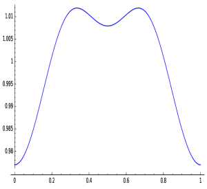
(a) A plot of of the invariant density

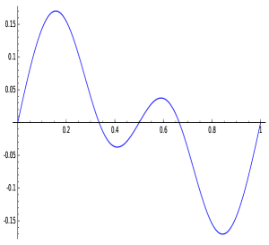
(b) The computed linear response

Figure 1. The computed approximations of the response in the stochastic case, and a plot of an approximation of the invariant density for the non-perturbed map.

In figure 1 a plot of the approximations of the invariant density and of the linear response of the map under stochastic perturbation are presented. We are going to estimate the error using the algorithm developed in the present paper (refer to Theorem 2.2 and the subsequent discussion):

$$||\hat{h}-\hat{h}_{appr}||_{\infty}\leq$$

$$||\sum_{i=l^{*}}^{+\infty}\mathcal{L}^{i}\hat{\mathcal{L}}h||_{\infty}+||\sum_{i=0}^{l^{*}-1}\mathcal{L}^{i}f_{\eta}-\sum_{i=0}^{l^{*}-1}\mathcal{L}^{i}_{\eta}f_{\eta}||_{\infty}+||\sum_{i=0}^{l^{*}-1}\mathcal{L}^{i}(f_{\eta}-\hat{\mathcal{L}}h)||_{\infty}.$$

In the following subsections we are going to estimate the different summands separately.

Remark 4.6.

To do our validated numerics we used SAGE [44] and the validated numerics packages shipped with it (the interval package is a binding to MPFI [40]), running either on local computers or on a cloud based version called Cocalc, https://cocalc.com/.

The discretized operators are computed using a rigorous interval Newton method [45], while the estimates for the norm of the discretized operators are done using Scipy [27], with rigorous error bounds on the error made by matrix-vector products, obtained through the implementation of the rigorous matrix-vector product of [43].

The experiment can be done on SageMathCloud following the SAGE worksheets contained in the software archive:

• stochastic_estimate_tail.sagews bounds the size of the tail $||\sum_{i=l^{*}}^{+\infty}\mathcal{L}^{i}\hat{\mathcal{L}}h||_{\infty}$;

• stochastic_C_1_part.sagews approximates the invariant density in the $C^{1}$ norm, to approximate $\hat{\mathcal{L}}h$;

• stochastic_final_estimate.sagews estimates the error on the linear response and computes the approximation.

The software package contains a subset of the project compinvmeas-python, a software package designed to approximate invariant measures and associated objects. There is a git repository for the full project whose access is by invitation: please send us an email so we can grant you access.

Part of the computation was done taking advantage of parallelization; to do so, some delicate memory issues arose [37].

4.4. Estimating $||\sum_{i=l^{*}}^{+\infty}\mathcal{L}^{i}\hat{\mathcal{L}}h||$

Let $\eta=1/262144$ and let $\mathcal{L}_{\eta}$ be the discretized operator; we have

(4.4) $$||\mathcal{L}_{\eta}^{9}|_{V_{C}^{0}}||_{\infty}\leq 9.39\cdot 10^{-5}$$

where $V_{C}^{0}=\{f\in{C}^{1},\int f=0\}$ is the set zero average densities, and for all $f\in{C}^{1}$, by the approximation Lemma 7.13:

$$||\mathcal{L}_{\eta}^{9}f-\mathcal{L}^{9}f||_{\infty}\leq 6.01\cdot 10^{-7}||f||_{{C}^{1}}+0.0021||f||_{\infty}.$$

We can bound the speed of convergence to equilibrium and the associated constants using the technique and the notation explained in subsection 7.7, with $n_{1}=9$ . For any $g$ in $V_{C^{0}}$, we have that, denoting by $g_{i}=\mathcal{L}^{7}g_{i-1}$:

$$\left(\begin{array}[]{c}||g_{i+1}||_{{C}^{1}}\\ ||g_{i+1}||_{\infty}\end{array}\right)\preceq\left(\begin{array}[]{cc}1.0006\cdot 10^{-8}&1.44\\ 6.01\cdot 10^{-7}&0.0022\end{array}\right)\left(\begin{array}[]{c}||g_{i}||_{{C}^{1}}\\ ||g_{i}||_{\infty}\end{array}\right),$$

which gives us the following estimates

$$||\mathcal{L}^{9k}f||_{\infty}\leq 1.00025(0.0024)^{k}||f||_{{C}_{1}}\quad||\mathcal{L}^{9k}f||_{\infty}\leq 4132.2(0.0024)^{k}||f||_{{C}_{1}}.$$

Therefore,

$$||\sum_{i=18}^{\infty}\mathcal{L}^{i}\hat{\mathcal{L}}h||_{\infty}\leq 0.00037\gamma.$$

Remark 4.7.

Note that in this Subsection the partition size is coarser than the ones used in Subsection 4.5 and 4.6; the reason is that estimating (4.4) is the most computationally expensive part of our algorithm.

Let $m=1/\eta$, the space of zero average measures of a partition of size $\eta$ has dimension $m-1$; the way we compute (4.4) rigorously is to choose a basis of the space of average zero measures and explicitly multiply a sparse matrix with each element of this basis, which implies that the computation time scales asymptotically as $m^{2}$ (see [20, Section 8.3] for a complete treatment in the $L^{1}$ case). Therefore, to speed up computations, it is worth computing (4.4) on a coarser partition and get information on $\mathcal{L}$ by using [21].

Since the first submission of the article we developed more efficient tecniques to estimate these bounds, using what we call “coarse-fine” estimates [19]. Since the article presenting these results is still a work in progress, we decided not to use them to do the computations in the present article, therefore the execution time of the examples is long but does not represent the state of the art of our theory.

4.5. Estimating $||\sum_{i=0}^{l^{*}-1}\mathcal{L}^{i}f_{\eta}-\sum_{i=0}^{l^{*}-1}\mathcal{L}^{i}_{\eta}f_{\eta}||_{\infty}$

Let $\eta=1/524288$, we have that

$$\begin{array}[]{cccc}N&||\mathcal{L}^{N}_{\eta}f_{\eta}||_{{C}^{1}}&N&||\mathcal{L}^{N}_{\eta}f_{\eta}||_{{C}^{1}}\\ 0&2.72&3&3.35\cdot 10^{-7}\\ 1&0.0007&4&1.07\cdot 10^{-8}\\ 2&1.44\cdot 10^{-5}&5&4.8\cdot 10^{-9}.\end{array}$$

We observe now that

$$||\mathcal{L}_{\eta}^{k}f||_{C^{1}}\leq 1.50002\cdot 0.261^{k}||f||_{C^{1}}+1.42||f||_{\infty},$$

which permits us to bound $||\mathcal{L}_{\eta}^{k}||_{C^{1}}$, and obtain that, for $6\leq N\leq 17$:

$$||\mathcal{L}_{\eta}^{N}f_{\eta}||_{C^{1}}\leq 8.67\cdot 10^{-9}$$

Therefore

$$||\sum_{i=0}^{17}\mathcal{L}^{i}f_{\eta}-\sum_{i=0}^{17}\mathcal{L}^{i}_{\eta}f_{\eta}||_{\infty}\leq 0.0018\gamma.$$

4.6. Estimating $||\sum_{i=0}^{l^{*}-1}\mathcal{L}^{i}(f_{\eta}-\hat{\mathcal{L}}h)||_{\infty}$

Let $\eta=1/524288$, we computed using the discretization in Subsections 7.4 and 7.5 an approximation $h_{\eta}$ of $h$ such that

$$||h-h_{\eta}||_{{C}^{1}}\leq 0.00022.$$

Therefore we have an approximation $f_{\eta}$ to $\hat{\mathcal{L}}h=\gamma h^{\prime}$ such that

$$||f_{\eta}-\gamma h^{\prime}||_{\infty}\leq 0.00022\gamma.$$

Therefore

$$||\sum_{i=0}^{17}\mathcal{L}^{i}(f_{\eta}-\hat{\mathcal{L}}h)||_{\infty}\leq 0.0047\gamma.$$

4.7. The error on the computed response

Therefore, the error on the response is

$$||\hat{h}-\hat{h}_{appr}||_{\infty}\leq\gamma(0.00037+0.0018+0.0047)\leq 0.0069\gamma.$$

5. Linear response for deterministic perturbations

We now consider deterministic perturbations of a $C^{3}$ expanding circle map $T_{0}$. Let

$$T_{\epsilon}(x)=T_{0}(x)+\epsilon S(x)+o_{C^{3}}(\epsilon);$$

where $S(x)\in C^{3}(\mathbb{T})$ and $o_{C^{3}}(\epsilon)$ is a term whose $C^{3}$ norm goes to $0$ faster than $\epsilon$ as $\epsilon$ goes to $0$. Under these assumptions (see for instance [5, 9, 23]), the operator

$$\hat{\mathcal{L}}f(x)=-\mathcal{L}_{0}\bigg{(}\frac{f\cdot S^{\prime}}{T^{\prime}_{0}}\bigg{)}(x)-\mathcal{L}_{0}\bigg{(}\frac{f^{\prime}\cdot S}{T^{\prime}_{0}}\bigg{)}(x)+\mathcal{L}_{0}\bigg{(}f\cdot S\cdot\frac{T^{\prime\prime}_{0}}{(T^{\prime}_{0})^{2}}\bigg{)}(x)$$

satisfies

$$\lim_{\epsilon\rightarrow 0}||\epsilon^{-1}(\mathcal{L}-\mathcal{L}_{\epsilon})f-\mathcal{\hat{L}}f||_{C^{1}}=0\leavevmode\nobreak\ \forall f\in C^{3},$$

where $\mathcal{L}_{\epsilon}$ is the Perron-Frobenius operator associated to $T_{\epsilon}$.

Remark 5.1.

If we suppose that the perturbation is small in the $C^{2}$ norm: $||T_{0}-T_{\epsilon}||_{C^{2}}\leq K\epsilon$ it follows that $\mathcal{L}_{\epsilon}$ and $\mathcal{L}$, satisfy a uniform Lasota-Yorke inequality. This implies that assumption (1) of Proposition 2.1 holds. Moreover, by [18], Section 6, assumption (2) and (3) of Proposition 2.1 also hold. Hence Proposition 2.1 holds and we have the linear response for these perturbations.

$$\lim_{\epsilon\rightarrow 0}||\frac{h_{\epsilon}-h}{\epsilon}-\hat{h}||_{\infty}=0,$$

where $\hat{h}:=(\textrm{Id}-\mathcal{L})^{-1}\mathcal{\hat{L}}h.$

5.1. An example of linear response under a deterministic perturbation

In this example we study a family $T_{\epsilon}$, $\epsilon\in[0,1)$ of $C^{3}$-small deterministic perturbations. We consider the family $T_{\epsilon}$:

$$T_{\epsilon}(x)=2x+\frac{\epsilon}{16}(\cos(4\pi x)+\frac{1}{4}\cos(8\pi x))\textrm{ mod $1$}.$$

For $\epsilon=0$ the dynamics is given by the map

$$T_{0}(x)=2x\textrm{ mod $1$};$$

whose invariant density $h$ is constant and equals to $1$. The operator $\mathcal{L}_{0}$, associated to $T_{0}$, satisfies the following inequalities:

$$\textrm{Var}(\mathcal{L}_{0}^{k}f)\leq\bigg{(}\frac{1}{2}\bigg{)}^{k}\textrm{Var}(f)$$

$$M=||\mathcal{L}_{0}||_{\infty}\leq 1$$

$$||\mathcal{L}_{0}^{k}f||_{C^{1}}\leq\bigg{(}\frac{1}{2}\bigg{)}^{k}||f||_{C^{1}}+||f||_{\infty}.$$

Note that the family satisfies the assumptions discussed in Remark 5.1. Hence the linear response formula can be applied. Following [23], the operator $\hat{\mathcal{L}}:C^{2}\to C^{1}$ is given by

(5.1) $$\hat{\mathcal{L}}h=\mathcal{L}_{0}\bigg{(}\frac{\pi}{8}\sin(4\pi x)+\frac{\pi}{16}\sin(8\pi x)\bigg{)}=\frac{\pi}{8}\sin(2\pi x)+\frac{\pi}{16}\sin(4\pi x)$$

and, by Proposition 2.1, the linear response is given by

$$\hat{h}=(\textrm{Id}-\mathcal{L}_{0})^{-1}\hat{\mathcal{L}}h=\sum_{i=0}^{+\infty}\mathcal{L}^{i}_{0}\hat{\mathcal{L}}h.$$

The simple structure of the example also allow to compute the response exactly.

Remark 5.2.

From direct computations we have that for all $\phi\in L^{1}$

$$\mathcal{L}_{0}\phi(x)=\frac{\phi(\frac{x}{2})+\phi(\frac{x}{2}+\frac{1}{2})}{2}.$$

Therefore, $\mathcal{L}_{0}\sin(2\pi x)=0$, $\mathcal{L}_{0}\sin(4\pi x)=\sin(2\pi x)$ and

$$\hat{h}=\sum_{i=0}^{+\infty}\mathcal{L}^{i}_{0}\hat{\mathcal{L}}h=\hat{\mathcal{L}}h+\mathcal{L}_{0}\hat{\mathcal{L}}h=\frac{1}{16}\left(3\pi\sin(2\pi x)+\pi\sin(4\pi x)\right).$$

We now approximate the linear response and estimate the error using the algorithm developed in the present paper (refer to Theorem 2.2 and the subsequent discussion). We will compute its linear response using the discretized operator and the general estimates introduced in Section 4. Let us set the discretization parameter $\eta=1/4194304$. We have:

$$||\hat{\mathcal{L}}h||_{\infty} \leq\frac{3\pi}{16};$$

$$||\hat{\mathcal{L}}h||_{C^{1}} \leq\frac{3\pi}{16}+\frac{\pi^{2}}{2}.$$

As $\hat{\mathcal{L}}h$ is explicit (see Equation 5.1) in the algorithm we use its discretization $f_{\eta}=\Pi_{\eta}\hat{\mathcal{L}}h$. Let us choose $l^{*}=57$ and approximate $\hat{h}$ by

$$\hat{h}_{appr}=\sum_{i=0}^{56}\mathcal{L}_{\eta}f_{\eta}.$$

In Figure 2 we have a plot of the approximated linear response $\hat{h}_{appr}$.

Now we apply the general procedure for the estimation of the error.

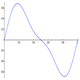
Figure 2. The plot of $\hat{h}_{appr}=\sum_{i=0}^{56}\mathcal{L}_{\eta}f_{\eta}$.

As in the previous section, we have to estimate three summands:

$$||\hat{h}-\hat{h}_{appr}||_{\infty}\leq$$

$$||\sum_{i=l^{*}}^{+\infty}\mathcal{L}^{i}\hat{\mathcal{L}}h||_{\infty}+||\sum_{i=0}^{l^{*}-1}\mathcal{L}^{i}f_{\eta}-\sum_{i=0}^{l^{*}-1}\mathcal{L}^{i}_{\eta}f_{\eta}||_{\infty}+||\sum_{i=0}^{l^{*}-1}\mathcal{L}^{i}(f_{\eta}-\hat{\mathcal{L}}h)||_{\infty}.$$

In the following we are going to estimate the different summands separately.

Remark 5.3.

The experiment can be done on SageMathCloud following the SAGE worksheets contained in the software archive:

• deterministic_estimate_tail.sagews bounds the size of the tail $||\sum_{i=l^{*}}^{+\infty}\mathcal{L}^{i}\hat{\mathcal{L}}h||_{\infty}$;

• deterministic_final_estimate.sagews estimates the error on the linear response and computes the approximation.

5.2. Estimating $||\sum_{i=l^{*}}^{+\infty}\mathcal{L}^{i}\hat{\mathcal{L}}h||$

Let us consider a coarse discretization $\eta=1/131072$ (see Remark 4.7) let $\mathcal{L}_{\eta}$ be its discretized operator. We have by direct computation

$$||\mathcal{L}_{\eta}^{19}|_{V_{C}^{0}}||_{\infty}\leq 0.00076$$

where $V_{C}^{0})=\{f\in{C}^{1},\int f=0\}$ is the set zero average densities. For all $f\in{C}^{1}$, by Lemma 7.13:

$$||\mathcal{L}_{\eta}^{19}f-\mathcal{L}^{19}f||_{\infty}\leq 0.000144||f||_{{C}^{1}}+0.0079||f||_{\infty}.$$

We can bound the speed of convergence to equilibrium and the associated constants using the technique and the notation explained in subsection 7.7, with $n_{1}=19$ . For any $g$ in $V_{C^{0}}$, we have that, denoting by $g_{i}=\mathcal{L}^{19}g_{i-1}$:

$$\left(\begin{array}[]{c}||g_{i+1}||_{{C}^{1}}\\ ||g_{i+1}||_{\infty}\end{array}\right)\preceq\left(\begin{array}[]{cc}1.91\cdot 10^{-6}&1\\ 0.000144&0.0079\end{array}\right)\left(\begin{array}[]{c}||g_{i}||_{{C}^{1}}\\ ||g_{i}||_{\infty}\end{array}\right).$$

This gives the following estimates for all $f\in V$

$$||\mathcal{L}^{19k}f||_{\infty}\leq 1.01(0.0171)^{k}||f||_{{C}_{1}}\quad||\mathcal{L}^{19k}f||_{\infty}\leq 120.1(0.0171)^{k}||f||_{{C}_{1}}.$$

Therefore,

$$||\sum_{i=57}^{\infty}\mathcal{L}^{i}\hat{\mathcal{L}}h||_{\infty}\leq 0.00055.$$

5.3. Estimating $||\sum_{i=0}^{l^{*}-1}\mathcal{L}^{i}f_{\eta}-\sum_{i=0}^{l^{*}-1}\mathcal{L}^{i}_{\eta}f_{\eta}||_{\infty}$

Let $\eta=1/4194304$, we have that

$$\begin{array}[]{cccc}N&||\mathcal{L}^{N}_{\eta}f_{\eta}||_{{C}^{1}}&N&||\mathcal{L}^{N}_{\eta}f_{\eta}||_{{C}^{1}}\\ 0&7.92&2&6.42\cdot 10^{-10}\\ 1&2.047&3&3.24\cdot 10^{-10}.\end{array}$$

We observe now that

$$||\mathcal{L}_{\eta}^{k}f||_{C^{1}}\leq 1.6\cdot 0.76^{k}||f||_{C^{1}}+1||f||_{\infty},$$

which permits us to bound $||\mathcal{L}_{\eta}^{k}||_{C^{1}}$, and obtain that, for $4\leq N\leq 56$:

$$||\mathcal{L}_{\eta}^{N}f_{\eta}||_{C^{1}}\leq 3.31\cdot 10^{-10}$$

Therefore,

$$||\sum_{i=0}^{56}\mathcal{L}^{i}f_{\eta}-\sum_{i=0}^{56}\mathcal{L}^{i}_{\eta}f_{\eta}||_{\infty}\leq 0.0019$$

5.4. Estimating $||\sum_{i=0}^{l^{*}-1}\mathcal{L}^{i}(f_{\eta}-\hat{\mathcal{L}}h)||_{\infty}$

Let $\eta=1/4194304$, we have that

$$||f_{\eta}-\hat{\mathcal{L}}h||_{\infty}=||\Pi_{\eta}(\hat{\mathcal{L}}h)-\hat{\mathcal{L}}h||_{\infty}\leq\frac{5}{2}\frac{1}{4194304}\frac{\pi^{2}}{2}\leq 2.96\cdot 10^{-6}.$$

Therefore,

$$||\sum_{i=0}^{56}\mathcal{L}^{i}(f_{\eta}-\hat{\mathcal{L}}h)||_{\infty}\leq 0.00017.$$

5.5. The error on the computed response

Therefore,

$$||\hat{h}-\hat{h}_{appr}||_{\infty}\leq 0.00055+0.0019+0.00017\leq 0.0026.$$

Remark 5.4.

We expect our approximation scheme to be more efficient than the rigorous bounds. Since we computed $\hat{h}$ explicitly in Remark 5.2, we compare our approximation directly with the explicit linear response obtaining:

$$||\hat{h}_{appr}-\Pi_{\eta}\hat{h}||_{C^{0}}\leq 3.42\cdot 10^{-13},\quad||\Pi_{\eta}\hat{h}-\hat{h}||_{C^{0}}\leq\frac{15.5}{4194304}.$$

This shows the efficiency of our approximation scheme.

6. Appendix I: the response of the intermittent family at the boundary

Let $T_{\alpha}:[0,1]\to[0,1]$ be the family of maps defined by

(6.1) $$T_{\alpha}(x)=\left\{\begin{array}[]{cc}x(1+2^{\alpha}x^{\alpha})&0\leq x\leq 1/2\\ 2x-1&1/2<x\leq 1,\end{array}\right.$$

where $\alpha\in[0,\infty)$. This family which was initially popularized in [33] as a version of the Pomeau-Manneville family [39]. When $\alpha\in(0,\infty)$, this family of maps of the interval $[0,1]$ has an indifferent fixed point at the origin, and when $\alpha\in(0,1)$ it has a unique absolutely continuous invariant probability measure and it exhibits only a polynomial decay of correlations [24] with respect to Hölder observables. When $\alpha=0$, it is the doubling map, which is uniformly expanding, it preserves Lebesgue measure and it exhibits exponential decay of correlations. In this appendix, we compute the linear response at $\alpha=0$.

In general for $\alpha\in[0,\infty)$, the transfer operator associated with $T_{\alpha}$ has a unique (up to multiplication by a constant) fixed point $h_{\alpha}\in L^{1}([0,1])$. The following result was proved in [11]. In particular, the linear response formula at $\alpha=0$ in Proposition 6.1 below was derived in equation (2.22) of [11].

Proposition 6.1.

Let $T_{\alpha}$ be as in (6.1) with $\alpha\in[0,1)$.

1. For $\alpha\in(0,1)$, $q>\frac{1}{1-\alpha}$ and $\psi\in L^{q}$

   (6.2) $$\lim_{\epsilon\to 0}\bigg{|}\frac{\int\psi h_{\alpha+\epsilon}dx-\int\psi h_{\alpha}dx}{\epsilon}-\int\psi\hat{h}_{\alpha}dx\bigg{|}=0,$$

   where $\hat{h}_{\alpha}=-(\textrm{Id}-\mathcal{L}_{\alpha})^{-1}[(X_{\alpha}\mathcal{N}_{\alpha}h_{\alpha})^{\prime}]$, with $X_{\alpha}=2^{\alpha}g_{0,\alpha}^{1+\alpha}(x)\ln(2g_{0,\alpha}(x))$, $\mathcal{N}_{\alpha}\varphi=g^{\prime}_{0,\alpha}(x)\varphi(g_{0,\alpha}(x))$.

2. The result also holds for $\alpha=0$ by taking the limit as $\epsilon\downarrow 0$. The formula of $\hat{h}:=\hat{h}_{0}$ is given by

   (6.3) $$\hat{h}=(\textrm{Id}-\mathcal{L}_{0})^{-1}\hat{\mathcal{L}}h_{0},$$

   where

   (6.4) $$\hat{\mathcal{L}}h_{0}=-1/4-\ln(x)/4\text{ and }h_{0}\equiv 1.$$

We now start the procedure of approximating $\hat{h}$ rigorously in $L^{1}([0,1])$. In this specific case, it is possible to find some explicit bounds that allow us to approximate the linear response. Note that approximating $\hat{h}$ in $L^{1}([0,1])$ will directly provide an approximation of $\int\psi\hat{h}dx$, for any $\psi\in L^{\infty}$. Since some of the techniques differ from those used in the rest of the paper, we decided to present this example as an appendix. Note that for $T_{0}(x)=2x\textrm{ mod $1$}$; the transfer operator on $L^{1}([0,1])$ associated to this dynamical system has the explicit form

$$\mathcal{L}_{0}f(x)=\frac{f(x/2)+f(x/2+1/2)}{2},$$

and the density of the absolutely continuous invariant measure is $h_{0}\equiv 1$; those are important ingredients in our estimates.

Remark 6.2.

The experiment can be done can be done on Cocalc following the SAGE worksheets contained in the software archive: lsv_at_boundary.sagews estimates the error on the linear response and computes the approximation.

Definition 6.3.

Let $\{I_{i}\}_{i=0}^{n-1}$ be a uniform partition of $[0,1]$ consisting of intervals of size $\eta=1/n$, denote by $m$ the Lebesgue measure. Let $\pi_{\eta}$ be the finite rank operator defined on $L^{1}([0,1])$ as follows:

$$\pi_{\eta}f(x)=\sum_{i=0}^{n-1}\frac{\int_{I_{i}}f\,dm}{m(I_{i})}\chi_{I_{i}}(x),$$

where $\chi_{I_{i}}$ is the characteristic function of $I_{i}$. The Ulam approximation of $\mathcal{L}_{0}$ of mesh size $\eta$ is

$$\mathcal{L}_{0,\eta}:=\pi_{\eta}\mathcal{L}\pi_{\eta}.$$

We summarize in the next lemma some properties of $\pi_{\eta}$, $\mathcal{L}_{0}$ and $\mathcal{L}_{0,\eta}$ used in this appendix; we refer to [4, 20] and references therein for proofs of these results.

Lemma 6.4.

Let $T_{0}(x)=2x\textrm{ mod $1$}$, let $\mathcal{L}_{0}$ be the associated transfer operator, and let $\mathcal{L}_{0,\eta}$ be the Ulam approximation of size $\eta$. Then

$$||g-\pi_{\eta}g||_{L^{1}} \leq\eta\cdot\text{Var}(g)$$

$$||\mathcal{L}_{0}||_{L^{1}}\leq 1 \quad||\mathcal{L}_{0,\eta}||_{L^{1}}\leq 1$$

$$\text{Var}(\mathcal{L}_{0}g)\leq\frac{1}{2}\text{Var}(g) \quad\text{Var}(\mathcal{L}_{0,\eta}g)\leq\frac{1}{2}\text{Var}(g),$$

for all $g\in BV([0,1])$.

We now approximate $\hat{h}$, which was defined in equations (6.3) and (6.4), with a rigorous error bound in $L^{1}([0,1])$.

Proposition 6.5.

Let $\mathcal{L}_{0,\eta}$ be the Ulam approximation of $\mathcal{L}_{0}$ with mesh size $\eta$. Let $\eta=2^{-20}$, $f_{\eta}=\pi_{\eta}\hat{\mathcal{L}}h_{0}$ and $\hat{h}_{appr}=\sum_{i=0}^{19}\mathcal{L}_{\eta}f_{\eta}$. Then,

$$||\hat{h}_{appr}-\hat{h}||_{L^{1}}\leq 0.00021.$$

Proof.

To obtain the rigorous bound for $||\hat{h}_{appr}-\hat{h}||_{L^{1}}$, note that

$$||\hat{h}_{appr}-\hat{h}||_{L^{1}} =||\sum_{i=0}^{19}\mathcal{L}_{0,\eta}^{i}f_{\eta}-(\textrm{Id}-\mathcal{L}_{0})^{-1}\hat{\mathcal{L}}h_{0}||_{L^{1}}\leq$$

$$||\sum_{i=0}^{19}\mathcal{L}_{0}^{i}(f_{\eta}- \hat{\mathcal{L}}h_{0})||_{L^{1}}+||\sum_{i=0}^{19}\mathcal{L}_{0}^{i}f_{\eta}-\sum_{i=0}^{19}\mathcal{L}^{i}_{0,\eta}f_{\eta}||_{L^{1}}+||\sum_{i=20}^{+\infty}\mathcal{L}^{i}_{0}\hat{\mathcal{L}}h_{0}||_{L^{1}}.$$

We will now give an explicit estimate for $||\mathcal{L}^{k}_{0}\hat{\mathcal{L}}h_{0}||_{L^{1}}$. By induction we have

$$|\mathcal{L}^{k}_{0}\hat{\mathcal{L}}h_{0}(x)|\leq|\bigg{(}-\frac{1}{4}-\frac{1}{4}\cdot\bigg{(}\frac{\ln(\prod_{j=1}^{2^{k}-1}(x+j))}{2^{k}}-\ln(2^{k})\bigg{)}\bigg{)}|+|\frac{\ln(x)}{2^{k+2}}|.$$

Note that if $x\in[0,1]$, we have that:

$$(2^{k}-1)!\leq\prod_{j=1}^{2^{k}-1}(x+j)\leq 2^{k}!;$$

we can use Stirling’s Formula for $n!$, [41]:

$$\ln(\sqrt{2\pi})+(n+\frac{1}{2})\ln(n)-n+\frac{1}{12n+1}\leq\ln(n!)\leq\ln(\sqrt{2\pi})+(n+\frac{1}{2})\ln(n)-n+\frac{1}{12n}.$$

Thus:

$$\bigg{|}1+\frac{\ln(\prod_{j=1}^{2^{k}-1}(x+j))}{2^{k}}-\ln(2^{k})\bigg{|}\leq\frac{\ln(\sqrt{2\pi})}{2^{k}}+\frac{\ln(2^{k})}{2^{k+1}}+\frac{1}{2^{2k}12},$$

which in turn implies that

$$||\mathcal{L}^{k}_{0}\hat{\mathcal{L}}h_{0}(x)||_{L^{1}}\leq\frac{1}{2^{k+2}}\cdot\bigg{(}1+\ln(\sqrt{2\pi})+\frac{\ln(2^{k})}{2}+\frac{1}{12\cdot 2^{k}}\bigg{)}.$$

Therefore,

(6.5) $$||\sum_{i=20}^{+\infty}\mathcal{L}^{i}_{0}\hat{\mathcal{L}}h_{0}||_{L^{1}}\leq\frac{1}{2^{20+1}}(1+\ln(\sqrt{2\pi}))+\frac{20+1}{2^{20+1}}\frac{\ln(2)}{2}+\frac{1}{9\cdot 2^{40+2}},$$

and consequently,

$$||\sum_{i=20}^{+\infty}\mathcal{L}^{i}_{0}\hat{\mathcal{L}}h_{0}||_{L^{1}}\leq 4.4\cdot 10^{-6}.$$

We estimate $||f_{\eta}-\hat{\mathcal{L}}h_{0}||_{L^{1}}$ explicitly:

$$\int_{0}^{\eta}|\ln(x)-\frac{\int_{0}^{\eta}\ln(x)dx}{\eta}|dx =\frac{2\eta}{e};$$

for each interval $[i\eta,(i+1)\eta]$, $i\in 1,\ldots,1/\eta-1$ we have that

$$\int_{i\eta}^{(i+1)\eta}|\ln(x)-\frac{1}{\eta}\int_{i\eta}^{(i+1)\eta}\ln(\xi)d\xi|dx\leq\eta(\ln(i\eta)-\ln((i+1)\eta)).$$

Therefore:

$$||f_{\eta}-\hat{\mathcal{L}}h_{0}||_{L^{1}}\leq\frac{\eta}{2e}-\frac{\eta\ln(\eta)}{4}.$$

Since $||\mathcal{L}_{0}||_{L^{1}}=1$ we have

(6.6) $$||\sum_{i=0}^{19}\mathcal{L}_{0}^{i}(f_{\eta}-\hat{\mathcal{L}}h_{0})||_{L^{1}}\leq 20\bigg{(}\frac{\eta}{2e}-\frac{\eta\ln(\eta)}{4}\bigg{)}.$$

Fix $\eta=2^{-20}$; therefore using (6.6) we have:

$$||\sum_{i=0}^{19}\mathcal{L}_{0}^{i}(f_{\eta}-\hat{\mathcal{L}}h_{0})||_{L^{1}}\leq 6.9\cdot{10^{-6}}$$

We bound now $||\sum_{i=0}^{19}\mathcal{L}_{0}^{i}f_{\eta}-\sum_{i=0}^{19}\mathcal{L}^{i}_{0,\eta}f_{\eta}||_{L^{1}}$. We make and “a priori” estimate, using the fact that $\eta=1/n$ and $\ln(x)$ is decreasing:

$$\text{Var}(f_{\eta})=\frac{|\int_{0}^{\eta}\hat{\mathcal{L}}h_{0}\,dx-\int_{(n-1)\eta}^{1}\hat{\mathcal{L}}h_{0}\,dx|}{\eta}=\frac{-\ln(\eta)-(n-1)\ln((n-1)\eta)}{4}$$

From Lemma 6.4

$$||(\mathcal{L}_{0}-\mathcal{L}_{0,\eta})f||_{L^{1}}\leq\frac{3\eta}{2}\text{Var}(f),$$

and

$$||\sum_{i=0}^{19}\mathcal{L}_{0}^{i}f_{\eta}-\sum_{i=0}^{19}\mathcal{L}^{i}_{0,\eta}f_{\eta}||_{L^{1}} \leq\sum_{j=0}^{19}\sum_{i=0}^{j}\frac{3\eta}{2}\bigg{(}\frac{1}{2}\bigg{)}^{i}\text{Var}(f_{\eta})$$

(6.7) $$\leq\frac{3\eta}{2}\bigg{(}2\cdot 20-\frac{2^{20}-1}{2^{19}}\bigg{)}\text{Var}(f_{\eta}).$$

Using (6.7), since for $\eta=2^{-20}$ $\text{Var}(f_{\eta})\leq 3.72$, we have the following bound:

$$||\sum_{i=0}^{19}\mathcal{L}_{0}^{i}f_{\eta}-\sum_{i=0}^{19}\mathcal{L}^{i}_{0,\eta}f_{\eta}||_{L^{1}}\leq 0.000203.$$

Summing up the errors we obtain:

$$||\hat{h}_{appr}-\hat{h}||_{L^{1}}\leq 0.00021.$$

∎

In Figure 3, we depict the graph of the computed approximation of the linear response.

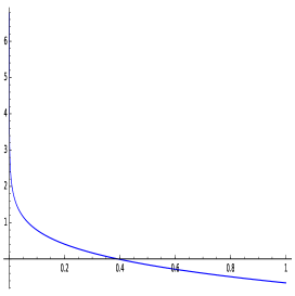
Figure 3. The plot of $\hat{h}_{appr}=\sum_{i=0}^{19}\mathcal{L}_{\eta}f_{\eta}$.

7. Appendix II: some estimates and technical lemmas

Throughout subsections 7.1-7.5 we use the following setup. $T:\mathbb{T}\rightarrow\mathbb{T}$ is a $C^{3}$ uniformly expanding circle map; i.e. $\inf_{x\in\mathbb{T}}|D_{x}T|>1$. Without loss of generality we assume that $T$ is orientation preserving. The circle map $T$ it is naturally associated with an expanding interval map, which we also denote by $T$, $T:[0,1]\to[0,1]$. Throughout the presentation, we use the interval map representation $T:[0,1]\to[0,1]$. Recall that $\mathcal{L}$ denotes the transfer operator associated with $T$ (see (3.1)). In addition, the following constants will be used extensively throughout subsections 7.1-7.5. We set

$$\lambda:=1/\inf_{x\in\mathbb{T}}|D_{x}T|;\quad B:=||T^{\prime\prime}/(T^{\prime})^{2}||_{\infty};\quad M:=1+\frac{B}{1-\lambda};$$

$$Z:=\frac{1}{1-\lambda^{2}}\bigg{(}\bigg{|}\bigg{|}\frac{T^{\prime\prime\prime}}{(T^{\prime})^{3}}\bigg{|}\bigg{|}_{\infty}+\frac{3\lambda}{1-\lambda}\bigg{|}\bigg{|}\frac{T^{\prime\prime}}{(T^{\prime})^{2}}\bigg{|}\bigg{|}_{\infty}^{2}\bigg{)};$$

and

$$D=\max\{3\frac{\lambda BM}{1-\lambda},3M\bigg{(}\frac{B}{1-\lambda}\bigg{)}^{2}+MZ\}+M\lambda+M^{2}.$$

Finally, we denote the $k^{\text{th}}$ iterate of $T$ by $G_{k}$; i.e. for $k\geq 1$ we write $G_{k}:=T^{k}$.

7.1. Useful estimates

The following Lemma provides bounds on the distortion for iterates of $T$. These bounds will be used in the proofs of the Lasota-Yorke inequalities in Subsection 7.2.

Lemma 7.1.

For any $k\geq 1$, we have

$$\bigg{|}\bigg{|}\frac{G_{k}^{\prime\prime}}{(G_{k}^{\prime})^{2}}\bigg{|}\bigg{|}_{\infty}\leq\frac{B}{1-\lambda};\quad\text{ and }\quad\bigg{|}\bigg{|}\frac{G_{k}^{\prime\prime\prime}}{(G_{k}^{\prime})^{3}}\bigg{|}\bigg{|}_{\infty}\leq Z.$$

Proof.

Write $G_{k}(x)=T(G_{k-1}(x))$. Then

$$G_{k}^{\prime}(x) =T^{\prime}(G_{k-1}(x))G_{k-1}^{\prime}(x),$$

$$G_{k}^{\prime\prime}(x) =T^{\prime\prime}(G_{k-1}(x))(G_{k-1}^{\prime}(x))^{2}+T^{\prime}(G_{k-1}(x))G_{k-1}^{\prime\prime}(x).$$

Using these two expressions we have

$$\frac{G^{\prime\prime}_{k}(x)}{(G_{k}^{\prime}(x))^{2}}=\frac{T^{\prime\prime}(G_{k-1}(x))}{(T^{\prime}(G_{k-1}(x)))^{2}}+\frac{1}{T^{\prime}(G_{k-1}(x))}\frac{G_{k-1}^{\prime\prime}(x)}{(G_{k-1}^{\prime}(x))^{2}},$$

which implies the first inequality. We now compute

$$G_{k}^{\prime\prime\prime}(x) =T^{\prime\prime\prime}(G_{k-1}(x))(G_{k-1}^{\prime}(x))^{3}+3T^{\prime\prime}(G_{k-1}(x))G_{k-1}^{\prime}(x)G_{k-1}^{\prime\prime}(x)$$

$$+T^{\prime}(G_{k-1}(x))G_{k-1}^{\prime\prime\prime}(x).$$

Using this last expression and the computations above we have:

$$\frac{G_{k}^{\prime\prime\prime}(x)}{(G_{k}^{\prime}(x))^{3}} =\frac{T^{\prime\prime\prime}(G_{k-1}(x))}{(T^{\prime}(G_{k-1}(x)))^{3}}+3\frac{1}{T^{\prime}(G_{k-1}(x))}\frac{T^{\prime\prime}(G_{k-1}(x))}{(T^{\prime}(G_{k-1}(x)))^{2}}\frac{G_{k-1}^{\prime\prime}(x)}{(G_{k-1}^{\prime}(x))^{2}}$$

$$+\frac{1}{(T^{\prime}(G_{k-1}(x)))^{2}}\frac{G_{k-1}^{\prime\prime\prime}(x)}{(G_{k-1}^{\prime}(x))^{3}},$$

which implies the second inequality of the lemma. ∎

7.2. Lasota-Yorke inequalities

In this subsection we prove Lasota-Yorke inequalities when $\mathcal{L}$ acts on $C^{1}([0,1])$ and on $C^{2}([0,1])$. The following proposition is a well known result. See for instance [32] Lemma 1.2 for a similar statement.

Proposition 7.2.

Let $\text{Var}(\cdot)$ denote the one dimensional variation on $[0,1]$. Then for any function of bounded variation $f$ we have

$$\text{Var}(\mathcal{L}f)\leq\lambda\text{Var}(f)+B||f||_{L^{1}}.$$

Lemma 7.3 (Uniform bound on $||\mathcal{L}^{n}||_{\infty}$).

For any $n\geq 1$ we have

$$||\mathcal{L}^{n}||_{\infty}\leq M.$$

Proof.

The operator $\mathcal{L}$ is positive. Therefore $||\mathcal{L}^{n}||_{\infty}=\sup_{x\in[0,1]}\mathcal{L}^{n}1.$ By Proposition 7.2, we have

$$\text{Var}(\mathcal{L}^{n}1)\leq\frac{B}{1-\lambda},$$

and therefore $||\mathcal{L}^{n}1||_{\infty}\leq M$. ∎

Proposition 7.4.

For $f\in C^{1}([0,1])$ and any $n\geq 1$ we have

$$||\mathcal{L}^{n}f||_{{C}^{1}}\leq M\cdot\lambda^{n}||f||_{{C}^{1}}+M^{2}||f||_{\infty}.$$

In particular, there exists an iterate $G:=T^{n}$ of $T$ such that

$$||\mathcal{L}_{G}f||_{{C}^{1}}\leq\theta||f||_{{C}^{1}}+M^{2}||f||_{\infty},$$

where $\theta\leq\lambda^{n}M<1$.

Proof.

For $x\in(0,1)$ we have

(7.1) $$\frac{\partial}{\partial x}(\mathcal{L}^{n}f)(x)=\frac{\partial}{\partial x}\bigg{(}\sum_{y\in G^{-1}(x)}\frac{f(y)}{G^{\prime}(y)}\bigg{)}=\sum_{y\in G^{-1}(x)}\frac{f^{\prime}(y)}{(G^{\prime}y)^{2}}-f(y)\frac{G^{\prime\prime}(y)}{(G^{\prime}y)^{2}}\frac{1}{G^{\prime}(y)}.$$

By Lemma 7.3, Lemma 7.1 and (7.1)

(7.2) $$||(\mathcal{L}^{n}f)^{\prime}||_{\infty}\leq\lambda^{n}||\mathcal{L}^{n}f^{\prime}||_{\infty}+\bigg{|}\bigg{|}\frac{G^{\prime\prime}}{(G^{\prime})^{2}}\bigg{|}\bigg{|}_{\infty}||\mathcal{L}^{n}f||_{\infty}\leq M\lambda^{n}||f^{\prime}||_{\infty}+\frac{BM}{1-\lambda}||f||_{\infty}.$$

Therefore, by (7.2) and Lemma 7.3, we have

$$\begin{split}||\mathcal{L}^{n}f||_{{C}^{1}}&=||\mathcal{L}^{n}f||_{\infty}+||(\mathcal{L}^{n}f)^{\prime}||_{\infty}\\ &\leq M||f||_{\infty}+M\lambda^{n}||f^{\prime}||_{\infty}+\frac{BM}{1-\lambda}||f||_{\infty}\\ &\leq M\lambda^{n}||f||_{{C}^{1}}+M^{2}||f||_{\infty}.\end{split}$$

∎

Proposition 7.5.

For $f\in C^{1}$, we have

$$||(\mathcal{L}f)^{\prime}||_{\infty}\leq(M+B)\lambda||f^{\prime}||_{\infty}+B(B+1)||f||_{L^{1}},$$

Proof.

From Proposition 7.2 and the fact that $||f||_{\infty}\leq||f||_{L^{1}}+\text{Var}(f)$ we have

$$||\mathcal{L}f||_{\infty}\leq\text{Var}(\mathcal{L}f)+||\mathcal{L}f||_{L^{1}}\leq\lambda\textrm{Var}(f)+(B+1)||f||_{L^{1}}$$

$$\leq\lambda||f^{\prime}||_{\infty}+(B+1)||f||_{L^{1}}.$$

By (7.2) and the above estimate we have

$$||(\mathcal{L}f)^{\prime}||_{\infty}\leq M\lambda||f^{\prime}||_{\infty}+B||\mathcal{L}f||_{\infty}\leq(M+B)\lambda||f^{\prime}||_{\infty}+B(B+1)||f||_{L^{1}}.$$

∎

Proposition 7.6.

For $f\in C^{2}([0,1])$ and any $n\geq 1$ we have

$$||\mathcal{L}^{n}f||_{{C}^{2}}\leq M(\lambda^{2})^{n}||f||_{{C}^{2}}+D||f||_{{C}^{1}}.$$

In particular, there exists an iterate $G:=T^{k}$ of $T$ such that

$$||\mathcal{L}_{G}f||_{{C}^{2}}\leq\Lambda||f||_{{C}^{2}}+D||f||_{{C}^{2}},$$

where $\Lambda\leq\lambda^{2k}M<1$.

Proof.

We denote $G:=T^{n}$. For $x\in(0,1)$ we have

$$(\mathcal{L}^{n}f)^{\prime\prime}(x)= \sum_{y\in G^{-1}(x)}\frac{f^{\prime\prime}(y)}{(G^{\prime}(y))^{3}}-3f^{\prime}(y)\frac{G^{\prime\prime}(y)}{(G^{\prime}(y))^{4}}$$

$$+\sum_{y\in G^{-1}(x)}-f(y)\frac{G^{\prime\prime\prime}(y)}{(G^{\prime}(y))^{4}}+3f(y)\frac{(G^{\prime\prime}(y))^{2}}{(G^{\prime}(y))^{5}}.$$

Therefore,

(7.3) $$||(\mathcal{L}^{n}f)^{\prime\prime}||_{\infty}\leq\lambda^{2n}||\mathcal{L}^{n}(f^{\prime\prime})||_{\infty}+3\lambda^{n}\frac{B}{1-\lambda}||\mathcal{L}^{n}(f^{\prime})||_{\infty}$$

$$+3\bigg{(}\frac{B}{1-\lambda}\bigg{)}^{2}||\mathcal{L}^{n}f||_{\infty}+Z||\mathcal{L}^{n}f||_{\infty}.$$

In particular

$$||(\mathcal{L}^{n}f)^{\prime\prime}||_{\infty}\leq M\lambda^{2n}||f^{\prime\prime}||_{\infty}+\max\{3\frac{\lambda^{n}BM}{1-\lambda},3M\bigg{(}\frac{B}{1-\lambda}\bigg{)}^{2}+MZ\}||f||_{{C}^{1}}.$$

Thus, by Proposition 7.4, we get

$$||\mathcal{L}^{n}f||_{{C}^{2}} =||\mathcal{L}^{n}f||_{{C}^{1}}+||(\mathcal{L}^{n}f)^{\prime\prime}||_{\infty}$$

$$\leq M\lambda^{2n}||f||_{{C}^{2}}$$

$$+\bigg{(}\max\{3\frac{\lambda^{n}BM}{1-\lambda},3M\bigg{(}\frac{B}{1-\lambda}\bigg{)}^{2}+MZ\}+M\lambda^{n}(1-\lambda^{n})+M^{2}\bigg{)}||f||_{{C}^{1}}.$$

∎

7.3. Uniform Lasota-Yorke inequality for $\mathcal{L}_{\eta}$

In this subsection we prove uniform Lasota-Yorke inequalities for the discretized operator defined $\mathcal{L}_{\eta}=\Pi_{\eta}\mathcal{L}\Pi_{\eta}$ that was defined in Subsection 3.2.

Proposition 7.7.

Let $0<\eta<\eta_{0}$. Suppose that

$$\Theta:=\bigg{(}\frac{3}{2}+6\eta_{0}\bigg{)}(M+B)\lambda<1.$$

For any $f\in C^{1}([0,1])$, and any $n\geq 1$, we have

$$||\mathcal{L}_{\eta}^{n}f||_{C^{1}}\leq(3+12\eta_{0})\bigg{(}\Theta^{n}||f||_{C^{1}}+\frac{B(B+1)}{1-\Theta}||f||_{1}\bigg{)}+||f||_{1},$$

and

$$||\mathcal{L}_{\eta}^{n}||_{C^{1}}\leq(3+12\eta_{0})\bigg{(}\Theta^{n}+\frac{B(B+1)}{1-\Theta}+\frac{1}{3}\bigg{)}.$$

Proof.

We start by bounding, using the inequality proved in Proposition 7.5

$$||(\mathcal{L}\Pi_{\eta}f)^{\prime}||_{\infty} \leq(M+B)\lambda||(\Pi_{\eta}f)^{\prime}||_{\infty}+B(B+1)||\Pi_{\eta}f||_{1}$$

$$\leq\bigg{(}\frac{3}{2}+6\eta\bigg{)}(M+B)\lambda||f^{\prime}||_{\infty}+B(B+1)||f||_{1}.$$

Since $||(\mathcal{L}\Pi_{\eta})^{n}f||_{1}=||f||_{1}$, we have that

$$||((\mathcal{L}\Pi_{\eta})^{n}f)^{\prime}||_{\infty}\leq\Theta^{n}||f^{\prime}||_{\infty}+\frac{B(B+1)}{1-\Theta}||f||_{1}.$$

Therefore,

$$||({\mathcal{L}}_{\eta}^{n}f)^{\prime}||_{\infty}\leq\bigg{(}\frac{3}{2}+6\eta\bigg{)}\bigg{(}\Theta^{n}||f^{\prime}||_{\infty}+\frac{B(B+1)}{1-\Theta}||f||_{1}\bigg{)}.$$

Since

$$||f||_{\infty}\leq||f||_{1}+\textrm{Var}(f)\leq||f||_{1}+||f^{\prime}||_{\infty}$$

we have

$$||\mathcal{L}_{\eta}^{n}f||_{C^{1}}\leq(3+12\eta)\bigg{(}\Theta^{n}||f^{\prime}||_{\infty}+\frac{B(B+1)}{1-\Theta}||f||_{1}\bigg{)}+||f||_{1}.$$

∎

7.4. Approximating the invariant density in the ${C}^{1}$ norm

In this subsection we provide a discretization scheme of the transfer operator $\mathcal{L}$ in order to approximate the invariant density of $T$ in the ${C}^{1}$ norm.

7.4.1. An approximation of $\mathcal{L}$ as an operator from $C^{2}\to C^{1}$.

Let

$$\phi(x)=\left\{\begin{array}[]{cc}1+10x^{3}+15x^{4}+6x^{5}&x\in[-1,0]\\ 1-10x^{3}+15x^{4}-6x^{5}&x\in[0,1]\\ 0&\textrm{otherwise}\end{array}\right.$$

and

$$\nu(x)=\left\{\begin{array}[]{cc}x-6x^{3}-8x^{4}-3x^{5}&x\in[-1,0]\\ x-6x^{3}+8x^{4}-3x^{5}&x\in[0,1]\\ 0&\textrm{otherwise}\end{array}\right..$$

Let $m\in\mathbb{N}$ and $\eta=1/m$. For $i=0,\dots,m$, let $a_{i}=i/m$, $\phi_{i}(x)=\phi(m\cdot x-i)$, $\nu_{i}(x)=\nu(m\cdot x-i)/m$. Let $\delta_{ij}=1$ if $i=j$ and $\delta_{ij}=0$ if $i\neq j$. The following relations hold for all $i$ and $j$:

$$\phi_{i}(a_{j}) =\delta_{ij},\quad\phi_{i}^{\prime}(a_{j})=0,\quad\phi_{i}^{\prime\prime}(a_{j})=0,$$

$$\nu_{i}(a_{j}) =0,\quad\nu_{i}^{\prime}(a_{j})=\delta_{ij},\quad\nu_{i}^{\prime\prime}(a_{j})=0.$$

Moreover, $\sum_{i=0}^{m}\phi_{i}(x)=1$; i.e., $\{\phi_{i}\}_{i=0}^{m}$ forms a partition of unity. Further, for $x\in[a_{i},a_{i+1}]$ we have

$$|\nu_{i}(x)|+|\nu_{i+1}(x)|\leq\frac{5}{16}\eta,\quad|\nu^{\prime}_{i}(x)|+|\nu^{\prime}_{i+1}(x)|\leq 1.$$

Furthermore, $\int_{0}^{1}\nu_{i}(x)=0$ for all $i=1,\ldots,m-1$. In addition we have,

(7.4) $$||\phi_{i}||_{\infty} =1,\quad||\phi_{i}^{\prime}||_{\infty}=\frac{15m}{8},\quad||\phi_{i}^{\prime\prime}||_{\infty}=\frac{10\sqrt{3}m^{2}}{3},$$

(7.5) $$||\nu_{i}||_{\infty} =\frac{16}{81m},\quad||\nu_{i}^{\prime}||_{\infty}=1,\quad||\nu_{i}^{\prime\prime}||_{\infty}=\frac{8m}{225}(28+19\sqrt{19})\leq 4m.$$

Let

$$\kappa(x)=6x(1-x).$$

Note that $\int_{0}^{1}\kappa(x)dx=1$. Let

(7.6) $$p(x)=\sum_{i=0}^{m}f(a_{i})\phi_{i}(x)+f^{\prime}(a_{i})\nu_{i}(x).$$

We define the operator

$$(\tilde{\Pi}_{\eta}f)(x):=p(x)+\bigg{(}\int_{0}^{1}fdx-\int_{0}^{1}pdx\bigg{)}\kappa(x).$$

For $f\in C^{2}([0,1])$, we prove in Lemma 7.10 estimates on the $C^{i}$, $i=0,1,2$, norms of $\tilde{\Pi}_{\eta}f$. We first start with two preliminary lemmas.

Lemma 7.8.

Let $f\in C^{2}([0,1])$, and let $p$ be as in (7.6).

1. $||p||_{\infty}\leq||f||_{\infty}+32/81||f^{\prime}||_{\infty}\eta$,

2. $||p^{\prime}||_{\infty}\leq 23/8||f^{\prime}||_{\infty}$,

3. $||p^{\prime\prime}||_{\infty}\leq 4||f^{\prime\prime}||_{\infty}$.

Proof.

In this proof, we will denote by $p_{i}(x):=p(x)|_{[a_{i},a_{i+1}]}$. By construction we have

$$p_{i}(x)=f(a_{i})\phi_{i}(x)+f(a_{i+1})\phi_{i+1}(x)+f^{\prime}(a_{i})\nu_{i}(x)+f^{\prime}(a_{i+1})\nu_{i+1}(x).$$

(1) follows by observing that:

$$|p_{i}(x)|\leq||f||_{\infty}|\phi_{i}(x)+\phi_{i+1}(x)|+||f^{\prime}||_{\infty}(|\nu_{i}(x)|+|\nu_{i+1}(x)|).$$

The proof of (2) relies on the fact that $(\phi_{i}(x)+\phi_{i+1}(x))^{\prime}=0$, since the $\phi_{i}$’s form a partition of the unity:

$$|p_{i}^{\prime}(x)|\leq|f(a_{i+1})-f(a_{i})||\phi^{\prime}_{i}(x)|+||f^{\prime}||_{\infty}$$

$$\leq\frac{15}{8}\frac{|f(a_{i+1})-f(a_{i})|}{\eta}+||f^{\prime}||_{\infty}.$$

We now prove (3). For $x\in[a_{i},a_{i+1}]$ let

$$l_{i}(x):=f(a_{i})+\frac{f(a_{i}+1)-f(a_{i})}{\eta}(x-a_{i}),\quad q_{i}(x):=p_{i}(x)-l_{i}(x);$$

we have $p_{i}^{\prime\prime}(x)=q_{i}^{\prime\prime}(x)$, where $q_{i}(a_{i})=q_{i}(a_{i+1})=0$. By unicity of polynomial representation, we have

$$q(x)=q^{\prime}(a_{i})\nu_{i}(x)+q^{\prime}(a_{i+1})\nu_{i+1}(x),$$

with

$$q^{\prime}(a_{i})=f^{\prime}(a_{i})-\frac{f(a_{i}+1)-f(a_{i})}{\eta},\quad q^{\prime}(a_{i+1})=f^{\prime}(a_{i+1})-\frac{f(a_{i}+1)-f(a_{i})}{\eta},$$

and

$$|q^{\prime\prime}(x)|\leq\frac{4}{\eta}(|q^{\prime}(a_{i})|+|q^{\prime}(a_{i+1}|).$$

In the last inequality we have used the fact that $|\nu^{\prime\prime}_{i}(x)|\leq 4/\eta$. Moreover,

$$|q^{\prime}(a_{i})|=|f^{\prime}(a_{i})-\frac{f(a_{i}+1)-f(a_{i})}{\eta}|=|f^{\prime}(a_{i})-f^{\prime}(a_{i})-f^{\prime\prime}(\xi)\eta/2|\leq\frac{||f^{\prime\prime}||_{\infty}\eta}{2},$$

which proves (3). ∎

The following lemma provides bounds on the distance, in $C^{i}$, $i=0,1,2$, between $f$ and $p$.

Lemma 7.9.

Let $f\in C^{2}([0,1])$, and let $p$ be as in (7.6).

1. $||f-p||_{\infty}\leq 15||f^{\prime}||\eta/8$,

2. $||f-p||_{\infty}\leq 3||f^{\prime\prime}||\eta^{2}/2$,

3. $||f^{\prime}-p^{\prime}||_{\infty}\leq 3||f^{\prime\prime}||\eta$,

4. $|\int_{0}^{1}(f-p)dx|\leq 15||f^{\prime}||\eta/8$,

5. $|\int_{0}^{1}(f-p)dx|\leq 3||f^{\prime\prime}||\eta^{2}/2$.

Proof.

Let $x\in[a_{i},a_{i}+1]$, we have $p_{i}(a_{i})=f(a_{i})$, $p^{\prime}(a_{i})=f^{\prime}(a_{i})$. We first prove (1). There exist $\xi,\varsigma\in[a_{i},a_{i+1}]$ such that:

$$|f(x)-p(x)|=|(f^{\prime}(\xi)-p^{\prime}(\varsigma))(x-a_{i})|\leq|||f^{\prime}||_{\infty}-||p^{\prime}||_{\infty}|\eta.$$

Thus, (1) follows from (2) of Lemma 7.8. We now prove (2). There exist $\xi,\varsigma\in[a_{i},a_{i+1}]$ such that:

$$|f(x)-p(x)|=|(f^{\prime\prime}(\xi)-p^{\prime\prime}(\varsigma))\frac{(x-a_{i})^{2}}{2}|\leq\frac{|||f^{\prime\prime}||_{\infty}-||p^{\prime\prime}||_{\infty}|}{2}\eta^{2}.$$

Thus, (2) follows from (3) of Lemma 7.8. We now prove (3); there exist $\xi,\varsigma\in[a_{i},a_{i+1}]$ such that:

$$|f^{\prime}(x)-p^{\prime}(x)|=|(f^{\prime\prime}(\xi)-p^{\prime\prime}(\varsigma))(x-a_{i})|\leq|||f^{\prime\prime}||_{\infty}-||p^{\prime\prime}||_{\infty}|\eta.$$

Thus, (3) follows from (3) of Lemma 7.8. Items (4) and (5) follow trivially from item (1) and (2). ∎

We now obtain estimates on the $C^{i}$, $i=0,1,2$ norms of $\tilde{\Pi_{\eta}}f$. First we need some notation that will be used in the remaining lemmas of this subsection. Fix $\eta_{0}>0$ and define the following constants

$$A_{1}:=\frac{23}{8}+\frac{32}{81}\eta_{0};\quad A_{2}:=4+\frac{32}{81}\eta+18\eta^{2}_{0};\quad A_{3}:=\frac{9}{4}+9.$$

Lemma 7.10.

Let $f\in C^{2}([0,1])$, then

1. $||\tilde{\Pi}_{\eta}f||_{\infty}\leq||f||_{\infty}+32/81||f^{\prime}||_{\infty}\eta+45||f^{\prime}||\eta/16$,

2. $||\tilde{\Pi}_{\eta}f||_{\infty}\leq||f||_{\infty}+32/81||f^{\prime}||_{\infty}\eta+9||f^{\prime\prime}||\eta^{2}/4$,

3. $||(\tilde{\Pi}_{\eta}f)^{\prime}||_{\infty}\leq 23/8||f^{\prime}||_{\infty}+45||f^{\prime}||\eta/4$,

4. $||(\tilde{\Pi}_{\eta}f)^{\prime}||_{\infty}\leq 23/8||f^{\prime}||_{\infty}+9||f^{\prime\prime}||\eta^{2}$,

5. $||(\tilde{\Pi}_{\eta}f)^{\prime\prime}||_{\infty}\leq 4||f^{\prime\prime}||_{\infty}+18||f^{\prime\prime}||\eta^{2}$.

Moreover, for all $\eta<\eta_{0}$ we have

$$||\tilde{\Pi}_{\eta}f||_{C^{2}}\leq A_{2}||f||_{C^{2}},\quad||\tilde{\Pi}_{\eta}f||_{C^{1}}\leq A_{1}||f||_{C^{1}}+A_{3}\eta^{2}||f||_{C^{2}}.$$

Proof.

By definition

$$\tilde{\Pi}_{\eta}f=p(x)+\int_{0}^{1}(f-p)dx\cdot\kappa(x).$$

We have $||\kappa||_{\infty}=3/2$, $||\kappa^{\prime}||_{\infty}=6$, $||\kappa^{\prime\prime}||_{\infty}=12$. Consequently, all the items in the lemma follow from Lemma 7.8 and items (4) and (5) of Lemma 7.9.

Finally, we have:

$$||\tilde{\Pi}_{\eta}f||_{C^{2}} \leq 4||f||_{C^{2}}+\frac{32}{81}\eta||f^{\prime}||_{\infty}+18||f^{\prime\prime}||\eta^{2}\leq(4+\frac{32}{81}\eta+18\eta^{2})||f||_{C^{2}};$$

$$||\tilde{\Pi}_{\eta}f||_{C^{1}} \leq\bigg{(}\frac{23}{8}+\frac{32}{81}\eta\bigg{)}||f||_{C^{1}}+\bigg{(}\frac{9}{4}+9\bigg{)}||f||_{C^{2}}\eta^{2},$$

which completes the proof of the lemma. ∎

7.5. Uniform Lasota-Yorke inequality for $\tilde{\mathcal{L}}_{\eta}$

We define now the discretized operator

$$\tilde{\mathcal{L}}_{\eta}:=\tilde{\Pi}_{\eta}\mathcal{L}\tilde{\Pi}_{\eta}.$$

In this subsection we prove uniform Lasota-Yorke inequalities for the discretized operator $\tilde{\mathcal{L}}_{\eta}$.

Proposition 7.11.

Let $0<\eta<\eta_{0}$. Suppose that

$$\Theta:=(M+B)\lambda(\frac{23}{8}+\frac{45}{4}\eta_{0})<1.$$

For any $n\geq 1$ we have

$$||(\mathcal{L}\tilde{\Pi}_{\eta})^{n}||_{C^{1}}\leq 2\Theta^{n}+\frac{B(B+1)}{1-\Theta}+1:=\tilde{K}$$

and

$$||\tilde{\mathcal{L}}_{\eta}^{n}||_{C^{1}}\leq 2(\frac{23}{8}+\frac{45}{4}\eta_{0})\bigg{(}\Theta+\frac{B(B+1)}{1-\Theta}+\frac{4}{23}\bigg{)}:=\tilde{M}.$$

Proof.

The proof is identical to the proof of Proposition 7.7, using the fact that $||(\tilde{\Pi}_{\eta}f)^{\prime}||_{\infty}\leq(\frac{23}{8}+\frac{45}{4}\eta)||f^{\prime}||_{\infty}$, which was proved in Lemma 7.10. ∎

Lemma 7.12.

Let $0<\eta<\eta_{0}$. Suppose that

$$\tilde{\Theta}:=A_{2}\cdot M\lambda^{2}+A_{3}\eta_{0}^{2}<1.$$

For $f\in C^{2}([0,1])$ and any $n\geq 1$ we have

$$||\tilde{\mathcal{L}}_{\eta}^{n}f||_{C^{2}}\leq A_{2}\tilde{\Theta}^{n}||f||_{C^{2}}+\frac{A_{2}DA_{1}\tilde{M}}{1-\tilde{\Theta}}||f||_{C^{1}},$$

where $\tilde{M}:=2(\frac{23}{8}+\frac{45}{4}\eta_{0})\bigg{(}\Theta+\frac{B(B+1)}{1-\Theta}+\frac{4}{23}\bigg{)}$.

Proof.

We bound

$$||\mathcal{L}\tilde{\Pi}_{\eta}f||_{C^{2}} \leq M\lambda^{2}||\tilde{\Pi}_{\eta}f||_{C^{2}}+D||\tilde{\Pi}_{\eta}f||_{C^{1}}$$

$$\leq(A_{2}\cdot M\lambda^{2}+A_{3}\eta^{2}_{0})||f||_{C^{2}}+D\cdot A_{1}||f||_{C^{1}}.$$

Then

$$||(\mathcal{L}\tilde{\Pi}_{\eta})^{n}f||_{C^{2}}\leq\tilde{\Theta}^{n}||f||_{C^{2}}+\frac{D\cdot A_{1}\tilde{M}}{1-\tilde{\Theta}}||f||_{C^{1}},$$

and

$$||\tilde{\mathcal{L}}^{n}f||_{C^{2}}\leq A_{2}\tilde{\Theta}^{n}||f||_{C^{2}}+\frac{A_{2}DA_{1}\tilde{M}}{1-\tilde{\Theta}}||f||_{C^{1}}.$$

∎

7.6. Some approximation inequalities

In this section we show how to control the error made in iterating the discretized transfer operator instead of the transfer operator, under the assumption that the dynamics satisfies a Lasota-Yorke inequality.

Lemma 7.13.

Suppose there are two norms $||\leavevmode\nobreak\ ||_{s}\geq||\leavevmode\nobreak\ ||_{w}$, such that $\forall f\in B_{s},\forall n\geq 1$

(7.7) $$||\mathcal{L}^{n}f||_{s}\leq A\lambda_{1}^{n}||f||_{s}+B||f||_{w}.$$

Let $\pi_{\delta}$ be a finite rank operator satisfying:

• $\mathcal{L}_{\delta}=\pi_{\delta}\mathcal{L}\pi_{\delta}$ with $||\pi_{\delta}f-f||_{w}\leq K\delta||f||_{s};$

• $\pi_{\delta}$, $\mathcal{L}^{i}$ and $\mathcal{L}_{\delta}^{i}$ are bounded for the norm $||\leavevmode\nobreak\ ||_{w}:$ $||\pi_{\delta}||_{w}\leq P$ and $\forall i>0$, $||\mathcal{L}^{i}||_{w}\leq M$, $||\mathcal{L}_{\delta}^{i}|_{V_{0}}||_{w}\leq C_{i}$, $i=0,\ldots,N$.

Then

$$||(\mathcal{L}^{n}-\mathcal{L}^{n}_{\delta})f||_{w} \leq K\delta\sum_{k=1}^{n}A\lambda_{1}^{k-1}C_{n-k}(A\lambda_{1}+PM)||f||_{s}$$

$$+ K\delta\sum_{k=1}^{n}C_{n-k}(A\lambda_{1}+PM+M)B||f||_{w}.$$

Proof.

We have

$$||(\mathcal{L}-\mathcal{L}_{\delta})f||_{w}\leq||\pi_{\delta}\mathcal{L}\pi_{\delta}f-\pi_{\delta}\mathcal{L}f||_{w}+||\pi_{\delta}\mathcal{L}f-\mathcal{L}f||_{w}.$$

Since

$$\pi_{\delta}\mathcal{L}\pi_{\delta}f-\pi_{\delta}\mathcal{L}f=\pi_{\delta}\mathcal{L}(\pi_{\delta}f-f),$$

and $||\pi_{\delta}f-f||_{w}\leq K\delta||f||_{s}$, we have

$$||\pi_{\delta}\mathcal{L}(\pi_{\delta}f-f)||_{w}\leq PM||\pi_{\delta}f-f||_{w}\leq PMK\delta||f||_{s}.$$

On the other hand

$$||\pi_{\delta}\mathcal{L}f-\mathcal{L}f||_{w}\leq K\delta||\mathcal{L}f||_{s}\leq K\delta(A\lambda_{1}||f||_{s}+B||f||_{w})$$

which gives

(7.8) $$||(\mathcal{L}-\mathcal{L}_{\delta})f||_{w}\leq K\delta(A\lambda_{1}+PM)||f||_{s}+K\delta B||f||_{w}$$

Now let us consider $(\mathcal{L}_{\delta}^{n}-\mathcal{L}^{n})f$. We have

$$||(\mathcal{L}_{\delta}^{n}-\mathcal{L}^{n})f||_{w} \leq \sum_{k=1}^{n}||\mathcal{L}_{\delta}^{n-k}(\mathcal{L}_{\delta}-\mathcal{L})\mathcal{L}^{k-1}f||_{w}\leq\sum_{k=1}^{n}C_{n-k}||(\mathcal{L}_{\delta}-\mathcal{L})\mathcal{L}^{k-1}f||_{w}$$

$$\leq K\delta\sum_{k=1}^{n}C_{n-k}(A\lambda_{1}+PM)||\mathcal{L}^{k-1}f||_{s}+C_{n-k}B||\mathcal{L}^{k-1}f||_{w}$$

$$\leq K\delta\sum_{k=1}^{n}C_{n-k}\bigg{(}(A\lambda_{1}+PM)(A\lambda_{1}^{k-1}||f||_{s}+B||f||_{w})+BM||f||_{w}\bigg{)}.$$

We will now collect the terms in front of $||f||_{s}$:

$$K\delta\sum_{k=1}^{n}A\lambda_{1}^{k-1}C_{n-k}(A\lambda_{1}+PM)||f||_{s},$$

and the terms in front of $||f||_{w}$:

$$K\delta\sum_{k=1}^{n}C_{n-k}(A\lambda_{1}+PM+M)B||f||_{w}.$$

∎

In the case where $f$ is a fixed point of $\mathcal{L}$ we have the following estimate:

Lemma 7.14.

Suppose there are two norms $||\leavevmode\nobreak\ ||_{s}\geq||\leavevmode\nobreak\ ||_{w}$, such that $\forall f\in B_{s},\forall n\geq 1$

(7.9) $$||\mathcal{\mathcal{L}}^{n}f||_{s}\leq A\lambda_{1}^{n}||f||_{s}+B||f||_{w}.$$

Let $\pi_{\delta}$ be a finite rank operator satisfying:

• $\mathcal{\mathcal{L}}_{\delta}=\pi_{\delta}\mathcal{\mathcal{L}}\pi_{\delta}$ with $||\pi_{\delta}f-f||_{w}\leq K\delta||f||_{s}$

• $\pi_{\delta}$, $\mathcal{\mathcal{L}}^{i}$ and $\mathcal{\mathcal{L}}_{\delta}^{i}$ are bounded for the norm $||\leavevmode\nobreak\ ||_{w}:$ $||\pi_{\delta}||_{w}\leq P$ and $\forall i>0$, $||\mathcal{\mathcal{L}}^{i}||_{w}\leq M$.

Then if $f$ is a fixed point of $\mathcal{\mathcal{L}}$, we have

$$||\mathcal{L}f-\mathcal{L}_{\delta}f||\leq K\delta(1+PM)||f||_{s}.$$

Proof.

The proof is almost identical to the one above:

$$||\mathcal{L}f-\mathcal{L}_{\delta}f||_{w}\leq||\mathcal{L}f-\pi_{\delta}\mathcal{L}f||_{w}+||\pi_{\delta}\mathcal{L}f-\pi_{\delta}\mathcal{L}\pi_{\delta}f||_{w},$$

since $f$ is fixed point:

$$||\mathcal{L}f-\mathcal{L}_{\delta}f||_{w} \leq||f-\pi_{\delta}f||_{w}+||\pi_{\delta}\mathcal{L}f-\pi_{\delta}\mathcal{L}\pi_{\delta}f||_{w}$$

$$\leq K\delta||f||_{s}+P||\mathcal{L}f-\mathcal{L}\pi_{\delta}f||_{w}$$

$$\leq K\delta||f||_{s}+PM||f-\pi_{\delta}f||_{w}$$

$$\leq K\delta||f||_{s}+PMK\delta||f||_{s}.$$

∎

7.7. A recursive convergence to equilibrium estimation for maps satisfying a Lasota-Yorke inequality

Here we recall an algorithm introduced in [21] to compute the convergence to equilibrium of a measure preserving system satisfying a Lasota-Yorke inequality. We will see how, the Lasota-Yorke inequality together with a suitable approximation of the transfer operator by a finite dimensional operator can be used to deduce finite time and asymptotic upper bounds on the contraction of the zero average space.

Consider two vector subspaces of the space of signed measures $B_{s}\subseteq B_{w}$ with norms $||\leavevmode\nobreak\ ||_{s}\geq||\leavevmode\nobreak\ ||_{w}$, suppose that the transfer operator $\mathcal{L}$ is such that $\forall f\in B_{s},\forall n\geq 1$

(7.10) $$||\mathcal{L}^{n}f||_{s}\leq A\lambda_{1}^{n}||f||_{s}+B||f||_{w}.$$

Let $\pi_{\delta}$ be a finite rank operator satisfying:

• $\mathcal{L}_{\delta}=\pi_{\delta}\mathcal{L}\pi_{\delta}$ with $||\pi_{\delta}f-f||_{w}\leq K\delta||f||_{s};$

• $\pi_{\delta}$, $\mathcal{L}^{i}$ and $\mathcal{L}_{\delta}^{i}$ are bounded for the norm $||\leavevmode\nobreak\ ||_{w}:$ $||\pi_{\delta}||_{w}\leq P$ and $\forall i>0$, $||\mathcal{L}^{i}||_{w}\leq M$, $||\mathcal{L}_{\delta}^{i}|_{V_{0}}||_{w}\leq\tilde{C}_{i}$, $i=0,\ldots,N$.

Then by Lemma 7.13 there exist $C(\delta,n),D(\delta,n)$ depending only on $\delta$ and $n$, such that

(7.11) $$||(\mathcal{L}_{\delta}^{n}-\mathcal{L}^{n})g||_{w}\leq C(\delta,n)||g||_{s}+D(\delta,n)||g||_{w}.$$

Suppose now that there exists an $n_{1}$ such that $||\mathcal{L}_{\delta}^{n_{1}}|_{V_{0}}||_{w}\leq\tilde{C}_{n_{1}}<1$; from now on, we will denote $\lambda_{2}=\tilde{C}_{n_{1}}<1$.

Let us consider a starting measure: $g_{0}\in V_{0}$, let us denote $g_{i+1}=\mathcal{L}^{n_{1}}g_{i}.$ If the system is as above, putting together the Lasota-Yorke inequality(7.10) and the approximation inequality (7.11)

(7.12) $$\left\{\begin{array}[]{c}||\mathcal{L}^{n_{1}}g_{i}||_{s}\leq A\lambda_{1}^{n_{1}}||g_{i}||_{s}+B||g_{i}||_{w}\\ ||\mathcal{L}^{n_{1}}g_{i}||_{w}\leq\lambda_{2}||g_{i}||_{w}+C(\delta,n_{1})||g_{i}||_{s}+D(\delta,n_{1})||g_{i}||_{w}\end{array}\right..$$

Writing (7.12) in a vector notation:

(7.13) $$\left(\begin{array}[]{c}||g_{i+1}||_{s}\\ ||g_{i+1}||_{w}\end{array}\right)\preceq\left(\begin{array}[]{cc}A\lambda_{1}^{n_{1}}&B\\ C(\delta,n_{1})&D(\delta,n_{1})+\lambda_{2}\end{array}\right)\left(\begin{array}[]{c}||g_{i}||_{s}\\ ||g_{i}||_{w}\end{array}\right)$$

where $\preceq$ indicates the component-wise $\leq$ relation (both coordinates are less or equal). The relation $\preceq$ can be used because the matrix is positive. The relation (7.13) and the assumptions allow to estimate explicitly the contraction rate, by approximating the matrix and its iterations. Let

$$\mathcal{M}=\left(\begin{array}[]{cc}A\lambda_{1}^{n_{1}}&B\\ C(\delta,n_{1})&D(\delta,n_{1})+\lambda_{2}\end{array}\right).$$

Consequently, we can bound $||g_{i}||_{s}$ and $||g_{i}||_{w}$ by a sequence

$$\left(\begin{array}[]{c}||g_{i}||_{s}\\ ||g_{i}||_{w}\end{array}\right)\preceq\mathcal{M}^{i}\left(\begin{array}[]{c}||g_{0}||_{s}\\ ||g_{0}||_{w}\end{array}\right)$$

which can be computed explicitly. This gives an explicit estimate on the speed of convergence for the norms $||\ ||$ and $||\ ||_{w}$ at a given time.

We need an asymptotic estimation as the one given in (2.2) and in particular an estimation for $C_{1}$ and $\rho.$ This can be done using the eigenvalues and eigenvectors of $\mathcal{M}.$

Indeed, let the leading eigenvalue be denoted by $\rho_{\mathcal{M}}$ and a left positive eigenvector $(a,b)$, such that $a+b=1$. For each pair of values by $(a,b)$ such that $a+b=1$. We can define a norm

$$||g||_{(a,b)}=a||g||_{s}+b||g||_{w}.$$

We have

$$||\mathcal{L}g||_{(a,b)}=a||\mathcal{L}g||_{s}+b||\mathcal{L}g||_{w}\leq(a,b)\cdot\mathcal{M}\cdot\left(\begin{array}[]{c}||g||_{s}\\ ||g||_{w}\end{array}\right).$$

Then

$$||\mathcal{L}^{kn_{1}}g||_{(a,b)}\leq\rho_{\mathcal{M}}^{k}||g||_{(a,b)}.$$

By estimating $\rho_{\mathcal{M}}$ and the vector $(a,b)$ we can have upper estimates on $C_{1}$ and $\rho.$

References

- [1] Bahsoun, W., Rigorous numerical approximation of escape rates, Nonlinearity 19 (11) (2006) pp. 2529-2542
- [2] Bahsoun, W., Bose, C., Invariant Densities and Escape Rates: Rigorous and Computable Approximations in The -norm, Nonlinear Anal., 74 (2011) pp. 4481-4495
- [3] Bahsoun, W. and Bose, C. and Duan, Y., Rigorous Pointwise approximations for invariant densities of nonuniformly expanding maps, Ergodic Theory Dynam. Systems 35 (2015) pp. 1028-1044
- [4] Bahsoun, W., Galatolo, S., Nisoli, I. and Niu, X., Rigorous approximation of diffusion coefficients for expanding maps, J. Stat. Phys. 163 (6) (2016) pp. 1486-1503
- [5] Bahsoun, W., Saussol, B., Linear response in the intermittent family: differentiation in a weighted -norm, Discrete Contin. Dyn. Syst. 36 (12) (2016) pp. 6657-6668
- [6] Baladi, V. The quest for the ultimate anisotropic Banach space, J. Stat. Phys. 166 (3-4) (2017) pp. 525-557
- [7] Baladi, V., Positive transfer operators and decay of correlations, Advanced Series in Nonlinear Dynamics, 16. World Scientific Publishing Co., Inc., River Edge, NJ, 2000. x+314 pp.
- [8] Baladi, V., On the susceptibility function of piecewise expanding interval maps, Comm. Math. Phys. 275 (3) (2007) pp. 839-859
- [9] Baladi, V., Linear response, or else, arXiv:1408.2937
- [10] Baladi, V., Smania, D., Linear response formula for piecewise expanding unimodal maps, Nonlinearity 21 (4) (2008) pp. 677-711
- [11] Baladi, V., Todd, M., Linear response for intermittent maps, Comm. Math. Phys. 347 (3) (2016), pp. 857-874
- [12] Carminati, C., Tiozzo, G., Tuning and plateaux for the entropy of -continued fractions, Nonlinearity 26 (2013) pp. 1049-1070
- [13] Dellnitz, M., Junge, O., On the approximation of complicated dynamical behavior, SIAM J. Numer. Anal. 36 (1999) pp. 491-515
- [14] Dolgopyat, D., On differentiability of SRB states for partially hyperbolic systems, Invent. Math. 155 (2) (2004) pp. 389-449
- [15] Froyland, G., Finite approximation of Sinai-Bowen-Ruelle measures for Anosov systems in two dimensions, Random Comput. Dynam. 3 (4) (1995) pp. 251-263
- [16] Froyland, G., Using Ulam’s method to calculate entropy and other dynamical invariants, Nonlinearity 12 (1) (1999) pp. 79-101
- [17] Froyland, G., Computer-assisted bounds for the rate of decay of correlations, Comm. Math. Phys. 189 (1) (1997) pp. 237-257
- [18] Galatolo, S. Statistical properties of dynamics. Introduction to the functional analytic approach, arXiv:1510.02615
- [19] Galatolo, S., Monge, M., Nisoli, I., Poloni F. Efficient recipes for the computation of invariant measures and other objects related to the statistical properties of dynamics, Work in Progress
- [20] Galatolo, S., Nisoli, I., An elementary approach to rigorous approximation of invariant measures, SIAM J. Appl. Dyn. Syst.13 (2) (2014) pp. 958-985
- [21] Galatolo, S., Nisoli, I. and Saussol, S., An elementary way to rigorously estimate convergence to equilibrium and escape rates, J. Comput. Dyn. 2 (1) (2015) pp. 51-64
- [22] Galatolo, S., Nisoli, I., Rigorous computation of invariant measures and fractal dimension for piecewise hyperbolic maps: 2D Lorenz like maps, Ergodic Theory Dynam. Systems 36 (6) (2016) pp.1865-1891
- [23] Galatolo S., Pollicott M, Controlling the statistical properties of expanding maps, Nonlinearity 30 (2017) pp. 2737-2751
- [24] Gouëzel, S., Sharp polynomial estimates for the decay of correlations, Israel J. Math. 139 (2004) pp. 29-65
- [25] Gouëzel, S., Liverani, C., Banach spaces adapted to Anosov systems, Ergodic Theory Dynam. Systems 26 (2006), pp. 189-217
- [26] Higham, N., The accuracy of floating point summation, SIAM Journal on Scientific Computing 14 (4) (1993) pp. 783-799
- [27] Jones E., Oliphant T., Peterson P. et Alia, SciPy: Open source scientific tools for Python,2001, http://www.scipy.org/
- [28] Katok, A., Knieper, G., Pollicott, M., Weiss, H., Differentiability and analyticity of topological entropy for Anosov and geodesic flows, Invent. Math. 98 (3) (1989) pp. 581-597
- [29] Keller, G., Liverani, C., Stability of the spectrum for transfer operators, Ann. Scuola Norm. Sup. Pisa Cl. Sci. (4) 28 (1) (1999) pp. 141-152
- [30] Korepanov, A. Linear response for intermittent maps with summable and nonsummable decay of correlations, Nonlinearity 29 (6) (2016) pp. 1735-1754
- [31] Liverani, C., Rigorous numerical investigation of the statistical properties of piecewise expanding maps. A feasibility study, Nonlinearity 14 (3) (2001) pp. 463-490
- [32] Liverani, C. Invariant measures and their properties. A functional analytic point of view. Dynamical systems. Part II, pp. 185-237, Pubbl. Cent. Ric. Mat. Ennio Giorgi, Scuola Norm. Sup., Pisa, 2003
- [33] Liverani, C., Saussol, B., Vaienti, S. A probabilistic approach to intermittency, Ergodic Theory Dynam. Systems 19 (1999), pp. 671-685
- [34] Lucarini, V., Blender, R., Herbert, C., Pascale, S., Wouters, J., Mathematical and Physical Ideas for Climate Science, Rev. Geophys. 52 (2014), pp. 809–859
- [35] Murray, R., Existence, mixing and approximation of invariant densities for expanding maps on , Nonlinear Anal. 45 (1) (2001), pp. 37-72
- [36] Murray, R., Ulam’s method for some non-uniformly expanding maps, Discrete Contin. Dyn. Syst. 26 (3) (2010) pp. 1007-1018
- [37] Nisoli, I., Memory handling of parallel computations on Cocalc, personal web page: http://www.im.ufrj.br/nisoli/blog/?p=131
- [38] Pollicott, M., Vytnova P., Linear response and periodic points, Nonlinearity 29 (10) (2016) pp. 3047-3066
- [39] Pomeau, Y., Manneville, P. Intermittent transition to turbulence in dissipative dynamical systems, Comm. Math. Phys. 74 (1980) pp. 189-197
- [40] Revol N., Rouillier F. Motivations for an arbitrary precision interval arithmetic and the MPFI library, Reliable Computing 11 (4) (2005) pp. 275-290
- [41] Robbins H., A Remark on Stirling’s Formula, The American Mathematical Monthly 62 (1) (1955) pp. 26-29
- [42] Ruelle, D., Differentiation of SRB states, Comm. Math. Phys. 187 (1997) pp. 227-241
- [43] Rump S.M. Fast and parallel interval arithmetic. BIT 39(3) (1999) pp. 539-560
- [44] The Sage Developers, SageMath, the Sage Mathematics Software System (Version 7.1), 2016, http://www.sagemath.org
- [45] Tucker W. Auto-Validating Numerical Methods (Frontiers in Mathematics), Birkhäuser 2010