Computational Bottlenecks of Quantum Annealing

A promising approach to solving hard binary optimisation problems is quantum adiabatic annealing (QA) in a transverse magnetic field. An instantaneous ground state — initially a symmetric superposition of all possible assignments of $N$ qubits — is closely tracked as it becomes more and more localised near the global minimum of the classical energy. Regions where the energy gap to excited states is small (e.g. at the phase transition) are the algorithm’s bottlenecks. Here I show how for large problems the complexity becomes dominated by $O(\log N)$ bottlenecks inside the spin glass phase, where the gap scales as a stretched exponential. For smaller $N$, only the gap at the critical point is relevant, where it scales polynomially, as long as the phase transition is second order. This phenomenon is demonstrated rigorously for the two-pattern Gaussian Hopfield Model. Qualitative comparison with the Sherrington-Kirkpatrick Model leads to similar conclusions.

Quantum algorithms offer hope for tackling computer science problems that are intractable for classical computers qcbook . However, exponential speed-ups seen in, e.g. number factoring shor , have not materialised for more difficult NP-complete problems np . Those problems are targeted by the quantum adiabatic annealing algorithm (QA) nishimori ; farhiX ; rmp . Any NP-hard problem can be recast as quadratic binary optimisation. QA solves it by implementing a quantum Hamiltonian, written with the aid of Pauli matrices as

$$\hat{H}=-\frac{1}{2}\sum_{i,k=1}^{N}J_{ik}\\ \hat{\sigma}_{i}^{z}\hat{\sigma}_{k}^{z}-\sum_{i=1}^{N}h_{i}\hat{\sigma}_{i}^{z}-\Gamma(t)\sum_{i=1}^{N}\hat{\sigma}_{i}^{x}.$$ (1)

Here the first two terms, diagonal in $z$-basis, encode the objective function. The last term represents the magnetic field in the transverse direction, which is decreased from $\Gamma(0)\gg 1$ to $\Gamma(T_{\text{ann}})=0$. The time $T_{\text{ann}}$ needed by the algorithm is determined by a condition that the annealing rate is sufficiently low to inhibit non-adiabatic transitions:

$$\mathrm{d}\Gamma/\mathrm{d}t\ll\Delta E\cdot\Delta\Gamma.$$ (2)

These are most likely near points where the instantaneous gap to excited states $\Delta E$ attains a minimum as a function of $\Gamma$; further, $\Delta\Gamma$ is defined as the width of the region where the gap remains comparable to its minimum value.

QA offers no worst-case guarantees on time complexity vandam , but initial assessments of typical case complexity were optimistic. Both experimental brooke and theoretical santoro evidence hinted at performance improvement over simulated annealing for finite-dimensional glasses; however, some empirical evidence in support of the theory has recently been called into question heim . Early exact diagonalisation studies also observed polynomially small gaps in the constraint satisfaction problem on random hypergraphs farhiSci , but that finding had been challenged by quantum Monte Carlo studies involving larger sizes young . Benchmarking of a hardware implementation of QA, courtesy of D-Wave Systems, shows no improvement in the scaling of the performance boixo ; ronnow . Whether that might be attributable to a finite temperature at which the device operates or its intrinsic noise is unclear at present boixo2 ; katzgraber ; zhu .

Statistical physics offer some intuitive guidance: Small gaps develop at the quantum phase transition point and become exponentially small when the transition is $1^{\text{st}}$-order partitioning ; qrem1 ; qrem2 ; kxor or when different parts of the system become critical at different times for strong-disorder continuous phase transitions fisher . The most promising candidates for QA are thus problems with bona fide $2^{\text{nd}}$-order phase transitions, where the disorder is irrelevant at the QCP.

The scaling analysis described here suggests a polynomially small gap at the critical point of the archetypal spin glass: the Sherrington-Kirkpatrick (SK) model sk1 ; sk2 ; sk3 . It has been pointed out santoro ; altshuler that QA may still be doomed by the bottlenecks in the spin glass phase. Exponentially small gaps away from the critical point have been observed in simulations farhigap , but adequate theoretical description of this phenomenon has proven challenging. A perturbative argument in support of this qualitative picture has been considered in ref. altshuler, . However, the results were not borne out by more accurate analysis that took into account the extreme value statistics of energy levels comment .

The present manuscript sheds new light on the mechanism of tunneling bottlenecks in the spin glass phase. Using exact, non-perturbative, methods, this is illustrated for a simple model, but the main findings are expected to be valid for quantum annealing of more realistic spin glasses. During annealing, the system must undergo a cascade of tunnelings at some specific values of $\Gamma_{1},\Gamma_{2},\ldots$ in an approximate geometric progression. For a finite system size, these bottlenecks are few, $O(\log N)$, and may not even appear until $N$ is sufficiently large, highlighting the challenge of interpreting the results of numerical studies. Bottlenecks also become increasingly easier as $\Gamma\to 0$, counter to expectations that tunnelings are inhibited as the model becomes more classical. A related finding is that the time complexity of QA is exponential only in some fractional power of problem size: a mild improvement over more pessimistic estimates altshuler .

Results

Summary. The spin glass phase, which is entered below some critical value of the transverse field $\Gamma_{c}$, is characterised by a large number of valleys. Often, this transition is abrupt, driven by competition between an extended state and a valley (localised state) with the lowest energy, as occurs in the random energy model qrem1 ; qrem2 . The exponentially small overlap between the two states then determines the gap at the phase transition. However, even if new valleys develop in a continuous manner as $\Gamma$ decreases, small changes in the transverse field may result in a chaotic reordering of associated energy levels, leading to Landau-Zener avoided crossings and attendant exponentially small gaps.

Nonetheless, attempts to make this intuition exact are fraught with potential pitfalls. For increasing $\Gamma$, two randomly chosen valleys are equally likely to come either closer together or further apart in energy. In the case of the former — and further, if the sensitivity of energy levels to changes in the transverse field is so large that the levels ‘collide’ before either valley disappears — avoided crossing will occur. This may not be necessarily the case when one considers ‘collisions’ with the ground state, which are of particular concern to QA. The ground state corresponds to a valley with the lowest energy; this and other low-lying valleys obey fundamentally different statistics of the extremes.

A case in point is the analysis of ref. altshuler, , which develops perturbation theory in $\Gamma$. The classical limit ($\Gamma=0$) is used as a starting point; how that analysis might be extended to $\Gamma>0$ has also been discussed laumann . A type of constraint satisfaction problem (CSP) has been considered: classical energy levels are discrete non-negative integers (number of violated constraints) but have exponential degeneracy. ‘Zeeman splitting’ for $\Gamma>0$ scales as $\sqrt{N}$, which, for large problems, may be sufficient to overcome the $O(1)$ classical gap and cause avoided crossings of levels associated with different classical energies. Yet this trend disappears if only levels with the smallest energies (after splitting) are considered; these are relevant for avoided crossings with the ground state. This about-face is not immediately apparent, only coming into play for $N\gtrsim 100$, when the exponential degeneracy of the classical ground state sets in. It has, however, been confirmed with analytical argument and numerics comment . Consequently, arguments based on perturbation theory cannot be used to establish the phenomenon.

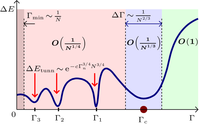
Figure 1: Sketch of the behavior of the gap in a Hopfield model with the Gaussian distribution of disorder variables: in the paramagnetic phase ($\Gamma>\Gamma_{c}$), in the glassy phase ($\Gamma<\Gamma_{c}$) and in the critical region ($\Gamma\approx\Gamma_{c}$). Scaling of the typical gap in these regions is indicated in bold letters using big-O notation. The area $\Gamma<\Gamma_{\text{min}}\sim 1/N$ is where the discrete nature of the energy landscape becomes manifest: the ground state becomes nearly completely localised. The glassy phase also contains $\log N$ isolated bottlenecks, indicated with red arrows, where the gaps scales as a stretched exponential.

This manuscript offers a fresh perspective, illustrated by studying quantum annealing of the Hopfield model. Mean-field analysis correctly describes thermodynamics if the number of random ‘patterns’ is small. The method is further extended to extract information about exact quantum energy levels. Importantly, the classical energy landscape is made much more complex by insisting that the distribution of disorder is Gaussian. Fig. 1 sketches a ‘phase diagram’ obtained for this model. For decreasing $\Gamma$ the gap changes as follows: (1) it is finite (does not scale with $N$) in the paramagnetic phase, $\Gamma>\Gamma_{c}$; (2) scales as $1/N^{1/3}$ in the narrow region of width $1/N^{2/3}$ around $\Gamma=\Gamma_{c}$; (3) increases slightly, with typical values scaling as $1/N^{1/4}$ for $\Gamma<\Gamma_{c}$. In addition, there are avoided crossings at isolated points $\Gamma_{1},\Gamma_{2},\ldots$, which is a manifestation of the transverse field chaos, demonstrated conclusively in this work.

The first non-trivial example requires two Gaussian patterns. In this case the ‘energy landscape’ is effectively one-dimensional, which greatly simplifies the analysis. The most important element of this analysis is accounting for the extreme value statistics associated with the valleys (local minima) having the lowest energies. To this end, the distribution of energies of the classical landscape must be conditioned so that they are never below the energy of the global minimum. This becomes feasible when reformulated as a continuous random process, in the limit $N\to\infty$.

This particular model is not as interesting from the computer science perspective, not least because it affords an efficient classical algorithm. It is sufficiently simple so that a complete quantitative analysis presented later on in the manuscript has been possible. Yet, the model captures the essential properties of the spin glass: its qualitative features directly apply to much more general models, including Sherrington-Kirkpatrick. The most important feature of the classical energy landscape is that exhibits fractal properties, which both ensures that hard bottlenecks are present in the spin glass phase and also governs their distribution. The role of the transverse field is to approximately coarse-grain it on scales determined by $\Gamma$, eliminating small barriers; thus the number of valleys decreases as $\Gamma$ grows. A specific random process, corresponding to the energy landscape of the ‘infinite’-size instance, will contain every possible realisation of itself at some ‘length scale’. Some realisations will contain high barriers that cannot be easily overcome; these will lead to tunneling bottlenecks.

This intuition can be used to immediately establish the scaling of the number of tunneling bottlenecks. Since the model contains no inherent length scale in the limit $N\to\infty$, it can be argued that the expected number of tunneling bottlenecks in a finite interval $[\Gamma_{1};\Gamma_{2}]$ should be a function of the ratio $\Gamma_{2}/\Gamma_{1}$. The logarithm is the only function that respects additivity, i.e. $\mathcal{N}_{\text{tunn}}([\Gamma_{1},\Gamma_{2}])=\mathcal{N}_{\text{tunn}}([\Gamma_{1};\Gamma^{\prime}])+\mathcal{N}_{\text{tunn}}([\Gamma^{\prime},\Gamma_{2}])$. To obtain the total number of bottlenecks, one considers the interval $[\Gamma_{\text{min}};\Gamma_{c}]$. Here $\Gamma_{c}\sim 1$ is the boundary of the spin glass phase. The lower cutoff, $\Gamma_{\text{min}}$, corresponds to the lowest energy scale of the classical model, which scales as an inverse power of system size, e.g. as $1/N$ for the Gaussian Hopfield model. In a sense, tunneling bottlenecks are connected to the $\Gamma=0$ ‘fixed point’ (note that the classical gap vanishes asymptotically). To summarize, the number of tunneling bottlenecks will grow as

$$\mathcal{N}_{\text{tunn}}\approx\alpha\ln N.$$ (3)

Locations (in $\Gamma$) will depend on specific disorder realisation, but self-similarity ensures that the successive ratios $\Gamma_{n}/\Gamma_{n+1}$ converge to a universal distribution.

This logarithmic rise is far weaker than a power law seen in some phenomenological models of temperature chaos tchpow and, as has been argued above, likely to be a universal feature. The prefactor is model-dependent; its numerical value can be used to estimate the minimum problem size for which the mechanism becomes relevant, via $\mathcal{N}_{\text{tunn}}\approx 1$. A value of $\alpha\approx 0.15$ is obtained for the problem at hand, so that additional bottlenecks become an issue for $N\gtrsim 1000$. Prior numerical studies similarly required large sizes before the exponentially small minimum gap was observed farhigap , and so far there has been no evidence of two or more exponentially small gaps coexisting. The slow, logarithmic increase of the expected number of bottlenecks is the most likely culprit.

A notable feature of these results is that tunnelings become progressively ‘easier’ as $\Gamma\to 0$ despite the fact that the model becomes more classical. Tunneling gaps increase as

$$\Delta E_{\text{tunn}}^{(n)}\sim\mathrm{e}^{-c\Gamma_{n}^{3/4}N^{3/4}}.$$ (4)

Notice that they cease to be exponentially small for $\Gamma\lesssim\Gamma_{\text{min}}$; at that point the ground state is already localised near the correct global minimum. The power law exponent for this stretched exponential is model-dependent, related to the scaling of barrier heights. These scale as $N^{1/2}$ for the Gaussian Hopfield model, which, together with $O(N)$ scaling of the effective mass, gives rise to the $N^{3/4}$ term in the exponent.

The finding that the gaps increase for smaller $\Gamma$ deserves explanation. Typically, valleys with similar energies differ by up to $N/2$ spin flips. This changes once lowest energies are considered: All spin configurations with energies less than $\epsilon$ above the global minimum are contained in a neighborhood of radius $O\bigl{[}(N\epsilon)^{2/3}\bigr{]}$, using Hamming distance as a metric. The problem is not rendered easy by the mere fact that the global minimum is so pronounced (although theoretical analysis inspired an efficient classical algorithm for the $p=2$ Hopfield network, briefly described later on). It does imply, however, that the ground state wavefunction does not jump chaotically: Every subsequent tunneling involves shorter distances, with $O(\Gamma N)$ spin flips, and achieves progressively better approximation to the true global minimum. Absent such a trend, annealing would be most difficult toward the end of the algorithm, when $\Gamma\sim 1/N$, and the minimum gap would exhibit less favorable exponential scaling altshuler .

In what follows, the model and its solution are described in greater detail. First, finite-size scaling of the ‘easy’ QCP bottleneck is linked to the thermodynamics of the phase transition. The next part goes beyond thermodynamics, considering small corrections to the extensive contribution to the free energy. The entire low-energy spectrum, which depends on disorder realisation, is mapped onto that of a simple quantum mechanical particle in a random potential. Finally, extreme value statistics is applied to investigate the properties of that random potential near its global minimum by mapping it to a Langevin process. This yields the distribution of hard bottlenecks in a universal regime ($\Gamma\ll 1$).

Quantum Hopfield network. Consider a model with rank-$p$ matrix of interactions and no longitudinal field ($h_{i}=0$): hopfield

$$J_{ik}=\frac{1}{N}\sum_{\mu=1}^{p}\xi_{i}^{(\mu)}\xi_{k}^{(\mu)}$$ (5)

(cf. $\operatorname{rk}J_{ik}=N$ for SK model), where $\xi_{i}^{(\mu)}$ are taken to be i.i.d. random variables of unit variance. The thermodynamics of this quantum Hopfield model has been worked out in great detail by Nishimori and Nonomura qhm . In fact, that study motivated the development of QA nishimori .

When $p$ is small ($J_{ik}\sim 1/N$), it is appropriate to replace local longitudinal fields with their mean values $h_{i}=\sum_{k}J_{ik}\langle\sigma_{k}^{z}\rangle$. The identity $\langle\sigma_{i}^{z}\rangle=h_{i}/\sqrt{\Gamma^{2}+h_{i}^{2}}$ is used to close this system of equations. For a transverse field below the critical value, $\Gamma<\Gamma_{c}=1$, there appears a non-trivial ($\mathbf{m}\neq 0$) solution to the self-consistency equation for the macroscopic order parameter, a vector with $p$ components:

$$\mathbf{m}=\frac{1}{N}\sum_{i=1}^{N}\boldsymbol{\xi}_{i}\left\langle\hat{\sigma}_{i}^{z}\right\rangle.$$ (6)

Here, the disorder variables are also written using vector notation: $\boldsymbol{\xi}_{i}=\bigl{(}\xi_{i}^{(1)},\ldots,\xi_{i}^{(p)}\bigr{)}$.

This model is equivalent to the Curie-Weiss (quantum) ferromagnet, which has a continuous phase transition characterised by a set of mean-field critical exponents. Two of these are particularly useful in the analysis of the annealing complexity: the one for the singular component of the ground state energy ($E_{0}^{\text{sing}}/N\propto|\gamma|^{a}$) as well as the dynamical exponent for the gap ($E_{1}-E_{0}\propto\gamma^{b}$), where $\gamma=\Gamma-\Gamma_{c}$ is the ‘distance’ from the critical point. These exponents are defined for the infinite system, yet fairly general heuristic analysis (see the Methods section) predicts finite-size scaling for the QCP bottleneck:

$$\Delta E_{c}\propto N^{-\frac{b}{a-b}},\qquad\Delta\Gamma_{c}\propto N^{-\frac{1}{a-b}}.$$ (7)

Substituting values $a=2$ and $b=1/2$ for the problem at hand, one may estimate the gap at the critical point and the width of the critical region to be $O(N^{-1/3})$ and $O(N^{-2/3})$ respectively.

Worse-than-any-polynomial complexity of quantum annealing might be expected for the first order phase transition, which exhibits no critical scaling (but see ref. polyfirst, for an exception). Another possibility is for the dynamical exponent to diverge at the infinite randomness QCP: the finite-size gap scales as $\exp\bigl{(}-c\sqrt{N}\bigr{)}$ in a random Ising chain fisher . For the Hopfield model, however, this scaling is polynomial, as the disorder is irrelevant at the critical point. More intriguing is the fact that these pessimistic scenarios are not found in SK spin glass either: the model is characterised by the same set of critical exponents, albeit with logarithmic corrections sk1 ; sk2 ; sk3 . These corrections to scaling increase the gap and, respectively, decrease the width of the critical region by a factor of $\log^{2/9}N$. Thus, as long as $T_{\text{ann}}\gtrsim N$, non-adiabatic transitions at the critical point should be suppressed. This presents a conundrum as SK model is known to be an NP-hard problem; finding a polynomial-time (even in typical case) quantum algorithm would be a surprising development. The heuristic analysis is clearly insufficient, but ‘digging’ deeper into a problem would require a more ‘microscopic’ analysis. In the following, the problem is mapped to ordinary quantum mechanics to uncover its low-energy spectrum that explicitly depends on a particular realisation of disorder, $\{\boldsymbol{\xi}_{i}\}$.

Exact low-energy spectrum. Mean-field theory can be derived in a more systematic manner via Hubbard-Stratonovich transformation. Finite-temperature partition function $Z(\beta)=\operatorname{Tr}\bigl{(}\mathrm{e}^{-\beta H}\bigr{)}$ can be written as a path integral over $\mathbf{m}(t)$, which now acquires a dependence on the imaginary time $0\leqslant t\leqslant\beta$, with periodic boundary conditions: $\mathbf{m}(\beta)=\mathbf{m}(0)$. The value of the integral is dominated by stationary paths corresponding to the minimum of an effective potential $\mathcal{V}(\mathbf{m})$. While the discussion above has been deliberately equivocal on the distribution of disorder variables, it is now instructive to contrast bimodal ($\xi_{i}^{(\mu)}=\pm 1$) and Gaussian choices. The shapes of the effective potential for both scenarios are depicted in Fig. 2.

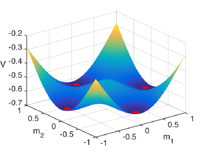
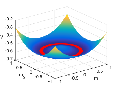
Figure 2: The shape of the disorder-averaged effective potential $\mathcal{V}(\mathbf{m})$ below the critical point ($\Gamma=0.5<\Gamma_{c}$) for the choice of bimodal (left) and Gaussian (right) distribution of disorder variables. Red color highlights the minimum of the potential. For the bimodal distribution, the $2p$-fold degenerate global minima are organised in pockets corresponding to encoded patterns. For Gaussian distribution, the degenerate minima form a continuum, connected by arbitrary rotations.

The conventional bimodal choice defines the model of associative memory: In the limit $\Gamma=0$ the ‘patterns’ can be perfectly recalled ($s_{i}=\pm\xi^{(\mu)}$) when $p$ is small. For the Gaussian choice, the global minimum corresponds to a mixture bovier

$$s_{i}=\pm\operatorname{sgn}\biggl{(}\sum_{\mu}\alpha_{\mu}\xi_{i}^{(\mu)}\biggr{)},$$ (8)

rendering memory useless. In the bimodal case, such ‘spurious’ states only become stable once the number of patterns scales with the problem size nnbook : $p>0.05N$. The $\textrm{BC}_{p}$ (bimodal) or $\textrm{O}(p)$ (Gaussian) symmetry of the effective potential is only approximate, to leading order in $N$. The degeneracy of the ground state is 2 (due to global spin inversion symmetry) for almost all disorder realisations when $p\geqslant 3$ or $p\geqslant 2$ in the bimodal and Gaussian scenarios respectively. (Note that that the $p=2$ bimodal case possesses an additional symmetry, which makes the ground state 4-fold degenerate.) The system is in a symmetric superposition of the degenerate global minima at the end of QA. It evolves entirely in the symmetric subspace since the time-dependent Hamiltonian commutes with $\hat{U}=\exp(\pi\mathrm{i}\hat{S}^{x})$. Thus, it should be noted that small gaps between symmetric and antisymmetric wavefunctions are irrelevant to QA and can be ignored.

Disorder fluctuations ‘nudge’ QA toward the ‘correct’ pattern as it passes the critical point in the bimodal Hopfield model. No further bottlenecks are encountered; gaps for $\Gamma<\Gamma_{c}$ as well as the ‘classical’ ($\Gamma=0$) gap are $O(1)$. By contrast, the classical gap scales as $O(1/N)$ in the Gaussian Hopfield model, alerting to a ‘danger’ posed by the $\Gamma=0$ ‘fixed point’. To find the low-energy spectrum when $\Gamma<\Gamma_{c}$, note that the dominant contribution to the path integral is from paths where the magnitude of the ‘magnetisation’ vector remains approximately constant, close to its saddle-point value, while the angle is a slow function of time: $\mathbf{m}(t)\approx m_{\Gamma}\bigl{(}\begin{smallmatrix}-\sin\vartheta(t)\\ \cos\vartheta(t)\end{smallmatrix}\bigr{)}$ for $p=2$. Integrating out the amplitude degrees of freedom, the partition function is rewritten as

$$Z(\beta)\propto\int[\mathrm{d}\vartheta(t)]\mathrm{e}^{-\int\limits_{0}^{\beta}\left(\frac{M}{2}\left(\frac{\mathrm{d}\vartheta}{\mathrm{d}t}\right)^{2}+V_{\Gamma}(\vartheta)\right)\mathrm{d}t},$$ (9)

which describes a quantum-mechanical particle of mass $M=O(N)$ moving on a ring, subjected to a random potential

$$V_{\Gamma}(\vartheta)=-\sum_{i}\sqrt{\Gamma^{2}+m_{\Gamma}^{2}\xi_{i}^{2}\sin^{2}(\vartheta-\theta_{i})}+N\left<\sqrt{\cdots}\right>_{\xi},$$ (10)

where $\boldsymbol{\xi}_{i}\equiv\xi_{i}\bigl{(}\begin{smallmatrix}\cos\theta_{i}\\ \sin\theta_{i}\end{smallmatrix}\bigr{)}$ and the last term, written in shorthand, adds a constant offset so that $\langle V(\vartheta)\rangle_{\boldsymbol{\xi}}=0$. Notice that $V_{\Gamma}(\vartheta)\propto\sqrt{N}$ via central limit theorem, thereby representing a higher-order correction to the extensive part of the free energy.

Since the partition function $Z(\beta)=\sum_{n}\mathrm{e}^{-\beta E_{n}}$ encodes information about the spectrum, low-energy (Goldstone) excitations of the many-body problem are in one-to-one correspondence with the energy levels of a quantum mechanical particle, up to a constant shift. The next step is to find the properties of this potential near a global minimum. These are relevant in a regime away from the critical point, $\Gamma\ll\Gamma_{c}$, where the universal behavior characterised by the appearance of ‘hard’ bottlenecks sets in.

Evolution of the random potential. Scaling of the gap for $\Gamma<\Gamma_{c}$ can be obtained via semiclassical analysis. Small level splitting due to tunneling between wells at the two degenerate global minima (this degeneracy is a consequence of the global $\mathrm{Z}_{2}$ symmetry: $V_{\Gamma}(\vartheta+\pi)=V_{\Gamma}(\vartheta)$) is not relevant to QA. Higher degeneracies are statistically unlikely; quantisation rules predict $O\bigl{(}N^{-1/4}\bigr{)}$ gaps between energy levels within the symmetric subspace. But this refers to the typical gap, obtained for fixed $\Gamma$ for almost all realisations of disorder. As quantum annealing sweeps the transverse field for a fixed realisation of disorder, $V_{\Gamma}(\vartheta)$ might undergo global bifurcation. This would result in a small tunneling gap for a specific value of $\Gamma$ when the competing minima are in resonance.

Such a scenario is impossible near the QCP. Coefficients in the Fourier expansion of the random potential, $\sum_{k}(a_{k}\cos 2k\vartheta+b_{k}\sin 2k\vartheta)$, decrease as $m^{2k}/\Gamma^{2k-1}$ so that the first harmonic dominates for $\Gamma\approx\Gamma_{c}$. Semiclassical analysis confirms a $O\bigl{(}N^{-1/3}\bigr{)}$ gap at the critical point (where the curvature of the effective potential vanishes, leaving only the quartic part). As $\Gamma$ decreases, the random potential becomes more rugged (see Fig. 4, left), smooth only on scales $\Delta\vartheta\sim\Gamma$, which makes global bifurcations more likely. Furthermore, it exhibits properties that allow one to make important predictions without detailed calculations. Rescaling the potential in the vicinity of either global minimum $V_{\Gamma}(\vartheta^{\ast})=V_{\Gamma}^{\ast}$,

$$\begin{split}\vartheta-\vartheta^{\ast}&\to\ell(\vartheta-\vartheta^{\ast}),\\ V_{\Gamma}-V_{\Gamma}^{\ast}&\to\ell^{3/2}(V_{\Gamma}-V_{\Gamma}^{\ast}),\end{split}$$ (11)

describes the same model but for the rescaled $\Gamma\to\ell\Gamma$ and a different realisation of disorder. This scale invariance is responsible for the logarithmic scaling of the number of tunneling bottlenecks as has been explained earlier in the text. However, it still remains necessary to demonstrate that the density of bottlenecks is non-zero, which entails an examination of the properties of the random potential in the limit $\Gamma=0$.

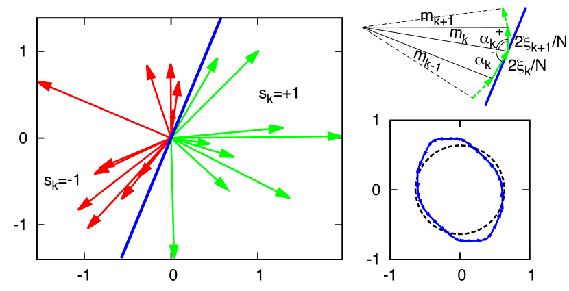
Figure 3: Geometric interpretation of the random potential, illustrated for a random instance with $N=20$. Vector $\mathbf{m}(\vartheta)$ is defined by drawing a separating line at angle $\vartheta$ and assigning spins with $\boldsymbol{\xi}_{i}$ on either side of separating line values $s_{i}=+1$ and $s_{i}=-1$ respectively (left figure). For changing $\vartheta$ vector $\mathbf{m}(\vartheta)$ is incremented/decremented by $(2/N)\boldsymbol{\xi}_{i}$ (top right). The increments form a closed path, approximated by a circle; fluctuations define a random potential (bottom right).

The classical optimisation problem corresponds to maximising the magnitude of $\sum_{i}\boldsymbol{\xi}_{i}s_{i}$. A necessary condition for a local minimum is that two sets of vectors, $\{\boldsymbol{\xi}_{i}|s_{i}=+1\}$ and $\{\boldsymbol{\xi}_{i}|s_{i}=-1\}$, can be separated by a line. As the angle of this line changes, fluctuations of the amplitude give rise to a random potential $V_{0}(\vartheta)$ (see Fig. 3). This suggests a linear-time algorithm for finding a global minimum: Sort all vectors by angle (this may introduce an extra $\log N$ factor due to sorting overhead) and exhaustively check all possible angles. Of course, QA algorithm is too generic to exploit the specific structure of the problem; moreover ad hoc efficient algorithms are unlikely to exist for more general spin glass problems.

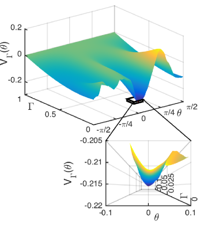
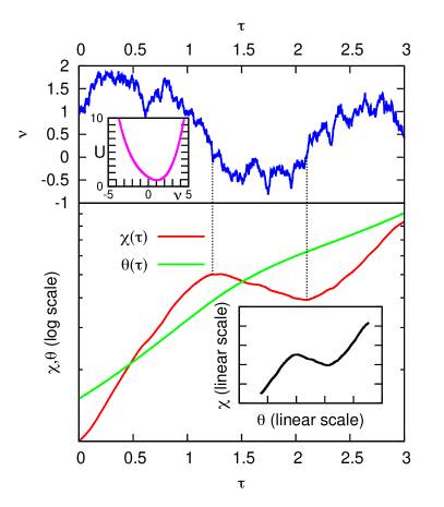
Figure 4: Illustration of appearance of local minima. Left: Potential $V_{\Gamma}(\theta)$ for a specific realisation of disorder as a function of $\Gamma$. A perspective-projection 3D plot that zooms on a region near the global minimum of $V_{0}(\theta)$ is shown in the bottom. Right: Top part of figure plots a specific realisation of a stochastic process $\nu(\tau)$ and a Langevin potential $\mathcal{U}(\nu)$ (inset). The bottom part integrates eqn. (12) to obtain $\chi(\tau)$ and $\vartheta(\tau)$ in the lower figure. Lower inset plots $\chi$ as a function of $\vartheta$. Regions with $\nu(\tau)<0$ are responsible for the appearance of local minima.

On short intervals, the random process is described as an undamped Langevin process sinai ; groeneboom in the continuous ($N\to\infty$) limit (hence the exponent of $3/2$ in eqn. (11), corresponding to its fractal dimension). Properly taking into account the statistics of the extremal properties, the process must be conditioned on the fact that $V_{0}(\vartheta)>V_{0}(\vartheta_{0}^{\ast})=V_{0}^{\ast}$ away from the global minimum. As described in Methods and the Supplement, such a conditioned process consists of two uncorrelated branches, $V_{0}(\vartheta)-V_{0}^{\ast}\propto\sqrt{N}\,\Bigl{\{}\begin{smallmatrix}\chi_{+},&\vartheta>\vartheta_{0}^{\ast},\\ \chi_{-},&\vartheta<\vartheta_{0}^{\ast}.\end{smallmatrix}$ Integrating equations

$$\begin{split}\mathrm{d}(\ln\chi_{\pm})/\mathrm{d}\tau&=\nu_{\pm}(\tau),\\ \mathrm{d}\vartheta/\mathrm{d}\tau&=\pm\chi_{\pm}^{2/3},\end{split}$$ (12)

defines $\chi_{+}(\vartheta)$ and $\chi_{-}(\vartheta)$ parametrically, in terms of random processes $\nu_{\pm}(\tau)$ that correspond to a Brownian motion in a non-linear potential depicted in Fig. 4. This potential is biased toward positive ‘velocities’ $\nu$ so that $V_{0}-V_{0}^{\ast}\sim\sqrt{N}(\vartheta-\vartheta^{\ast})^{3/2}$ from eqn. (12). It will, however, experience arbitrary percentage drops due to subpaths with $\nu<0$ (albeit with decreasing probability).

For small but finite $\Gamma$, the ‘separating line’ becomes blurred. The random potential adds a ‘quantum correction’ (see Methods and the Supplement), $V_{\Gamma}(\vartheta)-V_{0}(\vartheta)=O\bigl{(}\sqrt{N}\Gamma^{3/2}\bigr{)}$. For two minima to come into resonance, they cannot be more than $\Delta\vartheta\sim\Gamma$ apart (i.e. $O(N\Gamma)$ spin flips). The tunneling exponent is given by under-the-barrier action $\mathcal{A}\sim\sqrt{M\Delta V}\Delta\vartheta$, where the effective mass $M\sim N/\Gamma^{2}$ and $\Delta V\sim\sqrt{N}\Gamma^{3/2}$, leading to eqn. (4). Numerical results for the universal distribution of tunneling jumps and the tunneling exponents are exhibited in Fig. 5.

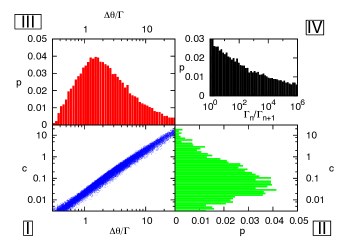
Figure 5: Numerical results. The L-shaped figure (composed of panels I-III) plots the distribution of the tunneling jumps and the exponent. The lower left quadrant (panel I) is a scatterplot of $\Delta\vartheta/\Gamma$ (proportional to the number of spin flips normalised by $\Gamma N$) against $|\log\Delta E_{\text{tunn}}|/(\Gamma N)^{3/4}$ (the prefactor $c$) for all tunneling events. Histograms of these quantities alone (projections of the scatterplot) are in the bottom right (panel II) and the top left (panel III) quadrants. The top right quadrant (panel IV) plots a histogram of distribution of $\Gamma_{n}/\Gamma_{n+1}$ for the successive tunneling events.

Discussion

Poor scalability of classical annealing of spin-glass models had been linked to the phenomenon of temperature chaos chaos . Interestingly, its existence in mean-field glasses had been debated tchsk1 ; rizzo ; tchsk2 , although it is uncontroversial in finite-dimensional models tchea1 ; tchea2 . Similarly, failures of quantum annealing might be attributed to transverse field chaos. The phenomenon described in this manuscript represents a much stronger finding. The mere fact that ground states at $\Gamma$ and $\Gamma+\Delta\Gamma$ will have vanishingly small overlap as $N\to\infty$ is not inconsistent with the continuously evolving ground state and poses no ‘threat’ to QA. By contrast, ‘hard’ bottlenecks correspond to isolated discontinuities that persist as $\Delta\Gamma\to 0$.

To dwell upon the generality of these results, first note that scaling of the tunneling exponent will depend on the universality class of the model. The SK model, for instance, exhibits different scaling of barrier heights, believed to be $\propto N^{1/3}$ (see e.g. ref. barriers, ). In the model studied, the decrease in the number of spins involved in tunnelings offsets the divergence of the effective mass in the classical limit $\Gamma\to 0$. As the height of the barriers also decreases, the tunneling gaps widen toward the end of the algorithm. One might expect qualitatively similar behavior in realistic spin glasses.

The logarithmic scaling of the number of bottlenecks is due to self-similar properties of the free energy landscape in the interval $[\Gamma_{\text{min}},\Gamma_{c}]$. The lower cutoff should correspond to the smallest energy scale in the classical limit, which for the SK model is also a negative power of $N$, namely $1/\sqrt{N}$. This is related to the linear vanishing of the density of distribution of effective fields as $h\to 0$ at zero temperature h0 (since $\int_{0}^{h_{\text{min}}}P(h)\mathrm{d}h\sim 1/N$). The picture is less clear for constraint satisfaction problems, where the energies are constrained to be non-negative integers; i.e. the classical gap is $O(1)$. These energy levels have exponential degeneracy, which is lifted by the transverse field. A value sufficient to make the spectrum effectively quasi-continuous might serve as an appropriate lower cutoff $\Gamma_{\text{min}}$ in problems of this type. Lack of ‘hard’ bottlenecks in the Hopfield model with the bimodal distribution of disorder and $p=O(1)$ could be attributed to the fact that the number of valleys is finite, which is not representative of a true spin glass.

An interesting observation is that since ‘hard’ bottlenecks correspond to Landau-Zener crossings, annealing times need not be exponentially small. The probability that QA fails to follow the ground state every single time in $n$ repeated experiments is

$$p_{\textrm{fail}}^{(n)}=\Bigl{(}\mathrm{e}^{-\frac{\pi\,\Delta E\cdot\Delta\Gamma}{4(\mathrm{d}\Gamma/\mathrm{d}t)}}\Bigr{)}^{n},$$ (13)

which exactly matches the probability of failure for the annealing rate that is $n$ times slower. Using shorter annealing cycles with many repetitions can minimize the effects of decoherence. It suffices that non-adiabatic transitions are suppressed at the critical point only, $\frac{\mathrm{d}\Gamma}{\mathrm{d}t}\lesssim 1/N$.

Even with polynomial annealing rates, coherent evolution would require much better isolation from the environment than what is currently feasible. The only commercial implementation of QA (D-Wave) must contend with a fairly strong coupling to a thermal bath. On the positive side, it accommodates faster annealing cycles, acting as a ‘safety valve’ to dissipate any heat generated during the non-adiabatic process. At the same time, it all but ensures that the system is always in thermal equilibrium with the environment.

The theory presented here breaks down when $\Gamma<T$ so that quantum bottlenecks described here may not be a limiting factor if $\ln(\Gamma_{c}/T)\lesssim 1/\alpha$. Main source of errors will be from exponentially many thermally occupied excited states. If the annealing profile were adjusted so that the energy spacing increased beyond $T$ towards the end, this would effectively implement classical annealing. An intricate relationship between temperature, problem size, and the properties of the spin glass model might determine which mechanism (quantum or classical annealing) will be dominant.

Yet another tradeoff in the design of D-Wave chip is a quasi-2D topology of interactions $J_{ik}$ due to fabrication constraints, which incurs significant performance penalty when mean-field models are ‘embedded’ into a ‘Chimera’ graph venturelli . So-called ‘native’ problems corresponding to uniformly random instances on this quasi-2D lattice have been argued to be poor candidates for QA due to the lack of a finite-temperature classical phase transition chimeraT0 ; at the same time, a quantum phase transition at $\Gamma_{c}>0$ is expected in 2D glasses quantum2d .

Whereas $1^{\text{st}}$-order phase transition immediately implies exponential complexity, even for small sizes, problems having a continuous phase transition may remain tractable up to a threshold, $N_{c}$, beyond which tunneling bottlenecks become dominant ($\alpha\ln N_{c}\sim 1$). This ‘tractability threshold’ serves as a silver lining fot this otherwise negative result. Moreover, the picture of ‘hard’ bottlenecks may be equally applicable to classical annealing. While in some crafted examples classical annealing is at a unique disadvantage due to $1^{\text{st}}$-order phase transition farhisa , for most interesting problems both classical and quantum transitions are $2^{\text{nd}}$-order. In such a scenario, the density of bottlenecks becomes a tie-breaker for evaluating relative performance. Whether quantum annealing can be advantageous in terms of this metric and determining which models will benefit is a practically important question for follow-up work.

There remains a question whether the failure mechanism described here can be somehow circumvented. Such a feat is feasible, e.g. for a disordered Ising chain, where an exponentially small gap develops at the critical point, which is a manifestation of Griffiths singularities fisher . Modification of QA that requires controlling the transverse field for each spin individually can suppress these singularities and restore a polynomial gap.

Based on comparison with another exactly solvable model, it seems that frustration — in addition to disorder — is essential for the appearance of small gaps in the spin glass phase proper. The seemingly random profile of the energy landscape for finite $\Gamma$ heralds difficulties in avoiding these bottlenecks in generic spin glasses. Although any prospects of exponential speedup should be met with skepticism, heuristics inspired by spin glass theory revolutionalised branch-and-bound algorithms for constraint satisfaction problems algo . One can remain hopeful that theoretical advances can similarly aid quantum optimisation.

Methods

Finite-size scaling of the gap at QCP is best understood using an example of a finite-dimensional system. In thermodynamic limit, both correlation length and characteristic time diverge near the phase transition as

$$\xi_{c}\propto(\Gamma-\Gamma_{c})^{-\nu},\qquad\tau_{c}\propto(\Gamma-\Gamma_{c})^{-z\nu}.$$ (14)

In a finite system this divergence is smoothed out as soon as the correlation length becomes comparable to lattice size ($\xi_{c}\sim N^{1/d}$). The minimum gap (the reciprocal of $\tau$) and the width of the critical region should scale as $N^{-z/d}$ and $N^{-1/(d\nu)}$ respectively. In this paper, the product $z\nu$ has been labeled as exponent $b$. Singular behavior of normalised ground state energy (free energy) is related to the specific heat exponent ($a=2-\alpha$). Dimensionality $d$ can be eliminated with the aid of hyperscaling relation $2-\alpha=(d+z)\nu$ to yield eqn. (7) of the main text. Independent estimates of the specific heat exponent can be obtained from the exponents for the order parameter and the susceptibility ($2-\alpha=2\beta+\gamma$).

Finite-temperature partition function can be written as a sum over a set of paths $[s_{i}(t)]$ with $0\leqslant t\leqslant\beta$, where $s_{i}(t)$ alternates between the values $\pm 1$. Hubbard-Stratonovich transformation can be used to rewrite it as a path integral

$$\begin{split}Z&\sim\sum_{[\{s_{i}(t)\}]}\mathrm{e}^{\frac{1}{2N}\int_{0}^{\beta}\left(\sum_{i}\boldsymbol{\xi}_{i}s_{i}(t)\right)^{2}\mathrm{d}t+\sum_{i}\mathcal{K}_{\Gamma}[s_{i}(t)]}\\ &\sim\int[\mathrm{d}\mathbf{m}(t)]\mathrm{e}^{-\frac{N}{2}\int_{0}^{\beta}\mathbf{m}^{2}(t)\mathrm{d}t+\sum_{i}\ln Z_{i}}.\end{split}$$ (15)

The ‘kinetic’ term $\mathcal{K}_{\Gamma}[s(t)]$ in the first equation penalises kinks, representing $\Gamma$-dependent ferromagnetic couplings between Trotter slices. As the interaction term is decoupled, the problem reduces to that of evaluating the single-site partition function $Z_{i}$ for a spin subjected to a magnetic field with the transverse component $\Gamma$ and the ‘time-dependent’ longitudinal component $h_{i}(t)=\boldsymbol{\xi}_{i}\mathbf{m}(t)$. To leading order in $N$, the saddle-point of the path integral (15) is a solution of mean-field equations. This becomes a degenerate manifold for Gaussian disorder distribution; to determine higher-order contribution all paths such that $|m(t)|=m_{\Gamma}$ are considered. Evaluating $Z_{i}$ is best performed in the adiabatic basis that diagonalises the 2-level Hamiltonian $\hat{H}_{i}=-h_{i}(t)\hat{\sigma}^{z}-\Gamma\hat{\sigma}^{x}$,

$$Z_{i}=\operatorname{Tr}\mathcal{T}\mathrm{e}^{\int_{0}^{\beta}\hat{H}_{i}(t)}\mathrm{d}t=\operatorname{Tr}\mathcal{T}\mathrm{e}^{-\int_{0}^{\beta}\left(\hat{E}_{i}(t)+\mathrm{i}\frac{\partial}{\partial t}\hat{V}_{i}(t)\right)\mathrm{d}t}.$$ (16)

Here $\hat{E}_{i}(t)$ is diagonal with eigenvalues $\pm\sqrt{\Gamma^{2}+h_{i}^{2}(t)}$. Its fluctuations around the mean give rise to the random potential $V_{\Gamma}(\vartheta)$. Non-adiabatic terms due to rotation of the basis ($\hat{U}=\mathrm{e}^{-\mathrm{i}\hat{V}_{i}(t)}$) are treated using 2nd order perturbation theory, giving rise to a kinetic term $\propto(\mathrm{d}\vartheta/\mathrm{d}t)^{2}$. Note a simple form of the perturbative term in eqn. (S7) owing to the fact that $\hat{V}_{i}(t)$ commute for all $t$.

In the limit $N\to\infty$, the random potential $V_{\Gamma}(\vartheta)$ defined in eqn. (10) in the main text converges to a Gaussian process that can be specified completely by its covariance matrix $\bigl{<}V_{\Gamma}(\vartheta)V_{\Gamma^{\prime}}(\vartheta^{\prime})\bigr{>}$. This can be ‘diagonalised’, alternatively expressing the random potential as a linear combination of white-noise processes $\{\zeta_{n}(\vartheta)\}$. One representation, as a convolution series $\sum_{n=0}^{\infty}\bigl{(}f_{\Gamma}^{(n)}\!\star\zeta_{n}\bigr{)}(\vartheta)$ with kernels

$$f_{\Gamma}^{(n)}(\vartheta)\propto\int_{0}^{\infty}\sqrt{\Gamma^{2}+\xi^{2}m_{\Gamma}^{2}\sin^{2}\vartheta}\;\xi^{\alpha+1}\mathrm{e}^{-\xi^{2}/2}L_{n}^{(\alpha)}\Bigl{(}\tfrac{\xi^{2}}{2}\Bigr{)}\mathrm{d}\xi,$$ (17)

relies on orthogonal properties of associated Laguerre polynomials. The choice $\alpha=1$ ensures that only $n=0$ term survives in the limit $\Gamma=0$. The random potential should satisfy a stochastic equation

$$\frac{\mathrm{d}^{2}V_{0}}{\mathrm{d}\vartheta^{2}}+V_{0}=\frac{2\sqrt{N}}{\pi}\zeta_{0}.$$ (18)

As a side note observe that a similar equation is obtained by taking a continuous limit in the identities that follow from elementary geometry (see Fig. 3 in the main text, $V_{k}=\frac{N}{2}m_{k}^{2}$):

$$\tfrac{V_{k+1}-V_{k}}{\xi_{k+1}}-\tfrac{V_{k}-V_{k-1}}{\xi_{k}}=\\ \tfrac{2}{N}(\xi_{k+1}+\xi_{k})+4\sqrt{2V_{k}/N}\cos\tfrac{\alpha_{k}^{+}-\alpha_{k}^{-}}{2}\cos\tfrac{\alpha_{k}^{+}+\alpha_{k}^{-}}{2}$$ (19)

For finite $\Gamma$, the form of the potential is modified as follows: It is convolved with a smoothing kernel of width $\Delta\vartheta\sim\Gamma$, which raises the global minimum by $O\bigl{(}\sqrt{N}\Gamma^{3/2}\bigr{)}$. Additional random contributions (from $n\geqslant 1$) have similar scaling.

In the vicinity of the global minimum, the statistics of the classical potential is fundamentally different. The ‘returning force’ in eqn. (18) can be neglected; additionally the process should be conditioned on the fact that it stays above its value at $\vartheta=0$ (no generality is lost by choosing the global minimum as the origin). This problem has been a subject of a considerable body of work sinai ; groeneboom , although important aspects ought to be revisited. Here, I present a particularly simple self-contained derivation.

A pair $(\chi,\upsilon)$ — where $\chi\propto V_{0}-V_{0}^{\ast}$ is interpreted as the ‘coordinate’ and $\upsilon=\mathrm{d}\chi/\mathrm{d}\vartheta$ as the ‘velocity’ ($\vartheta$ being ‘time’) — forms a Markov process. The probability distribution $p(\vartheta;\chi,\upsilon)$ satisfies, for $\vartheta>0$,

$$\frac{\partial p}{\partial\vartheta}=-\upsilon\frac{\partial p}{\partial\chi}+\frac{1}{2}\frac{\partial^{2}p}{\partial\upsilon^{2}},\quad\text{while }p(\vartheta;+0,\upsilon)=0\;(\forall\upsilon>0)$$ (20)

serves as a boundary condition for the absorbing boundary. This probability is ‘renormalised’ to condition on the fact that it survives until some $\Theta\gg\vartheta$. It becomes a conserved quantity, but the diffusion equation adds a drift, $-\partial(\log P_{\Theta})/\partial\upsilon$, repelling from the boundary. The ‘survival’ probability $P_{\Theta}$ in the limit $\Theta\to\infty$ is, up to ‘time-reversal’, the universal asymptotic solution of (20), reduced to ordinary differential equation (ODE) using scaling ansatz:

$$p(\vartheta,\chi,\upsilon)\propto\frac{\chi^{2\alpha/3}p_{\ast}\bigl{(}\upsilon\big{/}\chi^{1/3}\bigr{)}}{\vartheta^{\alpha}}.$$ (21)

This exploits a fact that fractal dimensions of ‘velocity’ and ‘coordinate’ are $[\upsilon]=[\vartheta]^{1/2}$ and $[\chi]=[\vartheta]^{3/2}$. The asymptotics is dominated by solutions with the smallest possible exponent, $\alpha=1/4$ out of the infinite set of eigenvalues for the ODE. This matches a known value obtained with a different method sinai .

The next step performs a change of variables, introducing ‘dimensionless’ velocity $\nu=\upsilon/\chi^{1/3}$, and ‘logarithmic’ coordinate $\mu=\ln\chi$. With the ‘time’ variable redefined via $\mathrm{d}\tau=\mathrm{d}\vartheta/\chi^{2/3}$, Markov process is described by a tuple $(\vartheta,\mu,\nu)$. Marginalising out $\mu$ and $\vartheta$ in the equation for $p(\tau;\vartheta,\mu,\nu)$ produces Fokker-Planck equation for a stochastic motion of particle in a potential

$$\mathcal{U}(\nu)=-\ln\left(\bigl{(}\nu/6^{1/3}\bigr{)}\operatorname{Ai}\bigl{(}\nu^{2}/6^{2/3}\bigr{)}+\operatorname{Ai}^{\prime}\bigl{(}\nu^{2}/6^{2/3}\bigr{)}\right).$$ (22)

Given a particular realisation of $\nu(\tau)$, the full process $(\mu,\nu,\vartheta)$ is determined deterministically, by integration (see eqn. (12) in the main text). The construction of a realisation of a random process is performed independently for $\vartheta>0$ and $\vartheta<0$.

Numerical simulations rescale this random potential instead of evolving the transverse field: $\vartheta\mapsto\mathrm{e}^{-\frac{\Delta\Gamma}{\Gamma}}\vartheta$ and $\chi\mapsto\mathrm{e}^{-\frac{3}{2}\frac{\Delta\Gamma}{\Gamma}}\chi$. The process is extended to larger values of $\tau$ as needed (details of the process for small $\tau$, where they fall below the numerical precision, are ‘forgotten’). A fairly large range of $\tau$ is required to gather the sufficient statistics.

The code used for simulations and the raw numerical results are available upon request.

Supplementary Information

Mathematical Preliminaries. This paper makes extensive use of Meijer G-function defined via intergal

$$G_{p,q}^{m,n}\biggl{(}z\bigg{|}\genfrac{}{}{0.0pt}{}{a_{1},\ldots,a_{n};a_{n+1},\ldots,a_{p}}{b_{1},\ldots,b_{m};b_{m+1},\ldots,b_{q}}\biggr{)}=\\ \frac{1}{2\pi\mathrm{i}}\int_{\mathcal{L}}\frac{\prod_{k=1}^{m}\boldsymbol{\Gamma}(b_{k}+s)\,\prod_{k=1}^{n}\boldsymbol{\Gamma}(1-a_{k}-s)}{\prod_{k=n+1}^{p}\boldsymbol{\Gamma}(a_{k}+s)\,\prod_{k=m+1}^{q}\boldsymbol{\Gamma}(1-b_{k}-s)}z^{-s}\mathrm{d}z,$$ (S1)

where the contour $\mathcal{L}$ is chosen appropriately. Bold $\boldsymbol{\Gamma}(x)$ is used to denote $\Gamma$-function to avoid confusion with the transverse field variable. G-function can be used to express many elementary and special functions; those used here include:

• $\mathrm{e}^{-x}=G_{0,1}^{1,0}\bigl{(}x\big{|}\genfrac{}{}{0.0pt}{}{-}{0}\bigr{)}$,

• $(1+x)^{-a}=\frac{1}{\boldsymbol{\Gamma}(a)}G_{1,1}^{1,1}\bigl{(}x\big{|}\genfrac{}{}{0.0pt}{}{1-a}{0}\bigr{)}$,

• $L_{n}^{(\alpha)}(x)\mathrm{e}^{-x}=\frac{1}{n!}G_{1,2}^{1,1}\bigl{(}x\big{|}\genfrac{}{}{0.0pt}{}{-n-\alpha}{0;-\alpha}\bigr{)}$,

• $U(a,b,x)=\frac{1}{\boldsymbol{\Gamma}(a)\boldsymbol{\Gamma}(a-b+1)}G_{1,2}^{2,1}\bigl{(}x\bigl{|}\genfrac{}{}{0.0pt}{}{1-a}{0,1-b}\bigr{)}$,

where $L_{n}^{(\alpha)}(x)$ are associated Laguerre polynomials and $U(a,b,x)$ represents confluent hypergeometric (Kummer) function. Multiplication by a finite power $x^{\alpha}$ merely shifts all parameters $a_{1},\ldots,a_{n},b_{1},\ldots,b_{m}$ by constant $\alpha$. Most integrals encountered can be recast as those of Mellin type:

$$\int_{0}^{\infty}G_{p,q}^{m,n}\biggl{(}\frac{x}{t}\bigg{|}\genfrac{}{}{0.0pt}{}{\vec{a}}{\vec{b}}\biggr{)}G_{r,s}^{k,\ell}\biggl{(}t\bigg{|}\genfrac{}{}{0.0pt}{}{\vec{c}}{\vec{d}}\biggr{)}\frac{\mathrm{d}t}{t}=G_{p+r,q+s}^{m+k,n+\ell}\biggl{(}x\bigg{|}\genfrac{}{}{0.0pt}{}{\vec{a},\vec{c}}{\vec{b},\vec{d}}\biggr{)},$$ (S2)

where vectors are concatenated as follows: $\vec{a},\vec{c}$ consists of $a_{1},\ldots,a_{n}$ and $c_{1},\ldots,c_{\ell}$ followed by $a_{n+1},\ldots,a_{p}$ and $c_{\ell+1},\ldots,c_{r}$ (similarly for $\vec{b}$ and $\vec{d}$). This ensures that zeros and poles in the Mellin transform of G-functions are grouped together.

Mean-Field Analysis. Self-consistency equation for the ‘magnetisation’ vector defined in eqn. (6) of the main text can be written as follows:

$$\mathbf{m}=\frac{1}{N}\sum_{i}\boldsymbol{\xi}_{i}\langle\sigma_{i}^{z}\rangle=\frac{1}{N}\sum_{i}\frac{\boldsymbol{\xi}_{i}(\boldsymbol{\xi}_{i}\mathbf{m})}{\sqrt{\Gamma^{2}+(\boldsymbol{\xi}_{i}\mathbf{m})^{2}}},$$ (S3)

where the individual spins polarise along the magnetic field with the components $\Gamma$ and $h_{i}=\boldsymbol{\xi}_{i}\mathbf{m}$ in the transverse and longitudinal directions respectively. Replacing sum over spins with disorder average, one obtains non-trivial solution to self-consistency equations for $\Gamma<1$. For the bimodal distribution, the solutions are $(\pm\sqrt{1-\Gamma^{2}},0,\ldots,0)$, $(0,\pm\sqrt{1-\Gamma^{2}},\ldots,0)$, etc. Other spurious solutions appear for smaller $\Gamma$, but they do not become stable for finite $p$. For Gaussian distribution, the magnetisation vector can have arbitrary direction while the magnitude $m_{\Gamma}$ satisfies

$$1=\int\tfrac{\xi^{2}}{\sqrt{\Gamma^{2}+\xi^{2}m_{\Gamma}^{2}}}\tfrac{1}{\sqrt{2\pi}}\mathrm{e}^{-\xi^{2}/2}\mathrm{d}\xi=\tfrac{1}{\sqrt{2}m_{\Gamma}}U\Bigl{(}\tfrac{1}{2},0;\tfrac{\Gamma^{2}}{2m_{\Gamma}^{2}}\Bigr{)},$$ (S4)

where the integral on the right hand side had been converted to Mellin type, $\int_{0}^{\infty}G_{1,1}^{1,1}\bigl{(}\frac{x}{t}\big{|}\genfrac{}{}{0.0pt}{}{1/2}{0}\bigr{)}G_{0,1}^{1,0}\bigl{(}t\big{|}\genfrac{}{}{0.0pt}{}{-}{1}\bigr{)}\frac{\mathrm{d}t}{t}$ by substituting $t=\xi^{2}/2$ and $x=\Gamma^{2}/(2m_{\Gamma}^{2})$. Alternatively, it can be expressed in terms of modified Bessel functions.

Low-energy spectrum of Hopfield model can be obtained by examining the partition function at finite temperature. It can be written as a sum over paths $[s_{i}(t)]$ alternating between values $s_{i}(t)=\pm 1$ with periodic boundary conditions $s_{i}(\beta)=s_{i}(0)$:

$$Z\sim\sum_{[\{s_{i}(t)\}]}\mathrm{e}^{\frac{1}{2}\int_{0}^{\beta}J_{ik}s_{i}(t)s_{k}(t)\mathrm{d}t+\sum_{i}\mathcal{K}_{\Gamma}[s_{i}(t)]}.$$ (S5)

The ‘kinetic’ term $\mathcal{K}[s(t)]=\text{(\# of kinks)}\times\frac{1}{2}\ln\coth\Gamma\Delta t$, where $\Delta t$ is the discretisation chosen (limit $\Delta t\to 0$ will be taken eventually). This term completely suppresses the dynamics in the limit $\Gamma=0$.

With $J_{ik}=(1/N)\sum_{\mu}\xi_{i}^{(\mu)}\xi_{k}^{(\mu)}$, two-body interactions are decoupled via Hubbard-Stratonovich transformation: Using the identity $\mathrm{e}^{\frac{1}{2N}\left(\sum_{i}\boldsymbol{\xi}_{i}s_{i}\right)}\propto\int\mathrm{d}\mathbf{m}\mathrm{e}^{-\frac{N}{2}\mathbf{m}^{2}+\sum_{i}\boldsymbol{\xi}_{i}\mathbf{m}s_{i}}$, the partition function is recast as a path integral,

$$Z\sim\int[\mathrm{d}\mathbf{m}(t)]\mathrm{e}^{-\frac{N}{2}\int_{0}^{\beta}\mathbf{m}^{2}(t)\mathrm{d}t+\sum_{i}\ln Z_{i}},$$ (S6)

where

$$Z_{i}=\sum_{[s(t)]}\mathrm{e}^{\int_{0}^{\beta}h_{i}(t)s_{i}(t)\mathrm{d}t+\mathcal{K}_{\Gamma}[s(t)]}=\operatorname{Tr}\mathcal{T}\mathrm{e}^{-\int_{0}^{\beta}\hat{H}_{i}(t)\mathrm{d}t}$$ (S7)

is a single-site partition function for a spin in a ‘time-dependent’ longitudinal field $h_{i}(t)=\boldsymbol{\xi}_{i}\mathbf{m}(t)$. It has been rewritten with the aid of time-ordering operator $\mathcal{T}$. The single-site Hamiltonian $\hat{H}_{i}(t)=-h_{i}(t)\hat{\sigma}^{z}-\Gamma\hat{\sigma}^{x}$.

The dominant contribution to the path integral is given by stationary paths, $\mathbf{m}(t)\equiv\mathbf{m}$. To leading order In this case $Z\sim\int\mathrm{d}\mathbf{m}\mathrm{e}^{-N\beta\mathcal{V}(\mathbf{m})}$, where the effective potential is

$$\mathcal{V}(\mathbf{m})=\tfrac{\mathbf{m}^{2}}{2}-\Bigl{<}\sqrt{\Gamma^{2}+(\boldsymbol{\xi}\mathbf{m})^{2}}\Bigr{>}_{\boldsymbol{\xi}}=\tfrac{\mathbf{m}^{2}}{2}-\sqrt{2}|\mathbf{m}|U\Bigl{(}-\tfrac{1}{2};0;\tfrac{\Gamma^{2}}{2\mathbf{m}^{2}}\Bigr{)}.$$ (S8)

The saddle-point value $m_{\Gamma}=|\mathbf{m}|$ that minimises the potential for $\Gamma=0$ is given by a solution of eqn. (S4).

Considering higher-order corrections, the dominant contribution comes from paths where the magnitude of magnetisation fluctuates around the mean-field value and the angle is a slow function of time: $\mathbf{m}(t)\approx m_{\Gamma}\bigl{(}\begin{smallmatrix}-\sin\vartheta(t)\\ \cos\vartheta(t)\end{smallmatrix}\bigr{)}$. Since the local field $h_{i}(t)$ is slow-varying, it is convenient to evaluate the partition function (S7) in the adiabatic basis that diagonalises the instantaneous 2-level Hamiltonian: $\hat{H}_{i}(t)=\mathrm{e}^{\mathrm{i}\hat{V}_{i}(t)}\hat{E}_{i}(t)\mathrm{e}^{-\mathrm{i}\hat{V}_{i}(t)}$ where

$$\hat{E}_{i}(t)=-\sqrt{\Gamma^{2}+h_{i}^{2}(t)}\,\hat{\sigma}^{z}\text{ and }\hat{V}_{i}(t)=\frac{1}{2}\operatorname{arccot}\frac{h_{i}(t)}{\Gamma}\hat{\sigma}^{y}.$$ (S9)

Using this factorisation, the time-ordered product $\operatorname{Tr}\bigl{(}\cdots\mathrm{e}^{\mathrm{i}\hat{V}_{i}(t+\Delta t)}\mathrm{e}^{-E_{i}(t+\Delta t)}\mathrm{e}^{-\mathrm{i}\hat{V}_{i}(t+\Delta t)}\mathrm{e}^{\mathrm{i}\hat{V}_{i}(t)}\mathrm{e}^{-E_{i}(t)}\mathrm{e}^{-\mathrm{i}\hat{V}_{i}(t)}\cdots\bigr{)}$ can be rewritten in the limit $\Delta t\to 0$ as

$$Z_{i}=\operatorname{Tr}\mathcal{T}\mathrm{e}^{-\int_{0}^{\beta}\left(\hat{E}(t)+\mathrm{i}\frac{\partial}{\partial t}\hat{V}(t)\right)\mathrm{d}t}$$ (S10)

The non-adiabatic term can be simply written as $\mathrm{i}\frac{\partial}{\partial t}\hat{V}(t)$ since all $\hat{V}(t)\propto\hat{\sigma}^{y}$ are commuting (should be $-U^{\dagger}\frac{\partial}{\partial t}U$ more generally) and acts as a perturbation. The lower-energy level, $E_{\downarrow}(t)=-\sqrt{\Gamma^{2}+h_{i}^{2}(t)}$, makes a dominant contribution to the partition function in the limit $\beta\to\infty$. Including second-order correction from the perturbation theory, $|\partial V_{\downarrow\uparrow}/\partial t|^{2}/(E_{\downarrow}-E_{\uparrow})$, one obtains:

$$\ln Z_{i}\approx\int_{0}^{\beta}\biggl{(}\sqrt{\Gamma^{2}+h_{i}^{2}}-\frac{\Gamma^{2}(\partial h_{i}/\partial t)^{2}}{8(\Gamma^{2}+h_{i}^{2})^{5/2}}\biggr{)}\mathrm{d}t.$$ (S11)

As the sum over all sites is performed, the first term in the integrand gives rise to a finite-size correction to the effective potential, which depends on angle $\vartheta$ and a particular realisation of disorder

$$V_{\Gamma}(\vartheta)=-\sum_{i}\sqrt{\Gamma^{2}+\xi_{i}^{2}m_{\Gamma}^{2}\sin^{2}(\vartheta-\theta_{i})}+N\Bigl{<}\sqrt{\Gamma^{2}+\xi^{2}m_{\Gamma}^{2}}\Bigr{>}_{\xi}.$$ (S12)

Vector-valued $\boldsymbol{\xi}_{i}$ has been parametrised here as $\xi_{i}\bigl{(}\begin{smallmatrix}\cos\vartheta(t)\\ \sin\vartheta(t)\end{smallmatrix}\bigr{)}$. Offsetting average in eqn. (S12) above has been made with respect to Gaussian distribution of the projection of $\boldsymbol{\xi}$ onto $\mathbf{m}$ (its value is independent of the direction). The second term in the integrand of eqn. (S11) contributes

$$\int_{0}^{\beta}\frac{1}{2}\underbrace{\sum_{i}\frac{\Gamma^{2}\xi_{i}^{2}m_{\Gamma}^{2}\cos^{2}(\vartheta-\theta_{i})}{4\left(\Gamma^{2}+\xi_{i}^{2}m_{\Gamma}^{2}\sin^{2}(\vartheta-\theta_{i})\right)^{5/2}}}_{M}\biggl{(}\frac{\mathrm{d}\vartheta}{\mathrm{d}t}\biggr{)}^{2}\mathrm{d}t.$$ (S13)

The ‘effective mass’ $M$ can be replaced by its average value

$$M=\frac{Nm_{\Gamma}}{4\sqrt{2}\Gamma^{2}}U\Bigl{(}\tfrac{1}{2},-1;\tfrac{\Gamma^{2}}{2m_{\Gamma}^{2}}\Bigr{)},$$ (S14)

which approaches $N\big{/}\bigl{(}4\sqrt{\pi}\Gamma^{2}\bigr{)}$ in the limit $\Gamma\to 0$. The dynamics becomes more classical as the effective mass diverges. Path integral (S6) is then rewritten as

$$Z\sim\mathrm{e}^{-N\beta\mathcal{V}(m_{\Gamma})}\int[\mathrm{d}\vartheta(t)]\mathrm{e}^{-\int_{0}^{\beta}\left(\frac{M}{2}\left(\frac{\mathrm{d}\vartheta}{\mathrm{d}t}\right)^{2}+V_{\Gamma}(\vartheta)\right)\mathrm{d}t}.$$ (S15)

The low-lying energy levels of the many-body problem are thus equivalent to those of a quantum mechanical particle on a ring.

The approximations made above break down for any finite $N$ when $\Gamma$ is sufficiently small. To avoid this, and to be able to make more quantitative predictions about the behavior of random potential (S12), it is necessary to study the continuous limit $N\to\infty$ directly.

Continuous Random Potential. Observe that the central limit theorem can be applied to the entire two-dimensional (in $\Gamma$ and $\vartheta$) process $V_{\Gamma}(\vartheta)$. This Gaussian process can be decorrelated by writing it as an infinite function series $V_{\Gamma}(\vartheta)=\sum_{n,m}\zeta_{nm}f_{nm}(\Gamma,\vartheta)$ involving independent Gaussian variables $\zeta_{nm}$. Basis functions are determined from the covariance $\langle V_{\Gamma}(\vartheta)V_{\Gamma^{\prime}}(\vartheta^{\prime})\rangle$. Since this correlation depends only on the angle difference $\vartheta-\vartheta^{\prime}$, it is natural to use $f_{nm}(\Gamma,\vartheta)=\tilde{f}_{nm}(\Gamma)\,\mathrm{e}^{\mathrm{i}m\vartheta}$.

Although the best truncated approximation is obtained by using Karhunen-Loève basis, there is no requirement that $\tilde{f}_{nm}(\Gamma)$ be orthogonal. In fact, since covariance involves averaging over distribution $\mathcal{P}(\xi)=\xi\,\mathrm{e}^{-\xi^{2}/2}$, it is quite convenient to use a set of polynomials that are orthogonal with said weight. Using a set of white noise processes

$$\bigl{<}\zeta_{n}(\vartheta)\,\zeta_{n^{\prime}}(\vartheta^{\prime})\bigr{>}=\delta_{nn^{\prime}}\,\delta(\vartheta-\vartheta^{\prime})\text{ for }\vartheta,\vartheta^{\prime}\in[-\pi/2;\pi/2],$$ (S16)

in lieu of discrete random variables, the series expansion becomes

$$V_{\Gamma}(\vartheta)=\sqrt{N}\sum_{n=0}^{\infty}\int_{-\pi/2}^{\pi/2}f_{\Gamma}^{(n)}(\vartheta-\theta)\,\zeta_{n}(\theta)\,\mathrm{d}\theta,$$ (S17)

where a factor $\sqrt{N}$ had been introduced for convenience. The convolution kernels should be chosen so as to match the covariance. One suitable choice is

$$f_{\Gamma}^{(n)}(\vartheta)=A_{n}\!\int_{0}^{\infty}\!\sqrt{\Gamma^{2}+m_{\Gamma}^{2}\xi^{2}\sin^{2}\vartheta}\,\xi^{\alpha+1}\mathrm{e}^{-\xi^{2}/2}L_{n}^{(\alpha)}\!\Bigl{(}\tfrac{\xi^{2}}{2}\Bigr{)}\mathrm{d}\xi.$$ (S18)

Since associated Laguerre polynomials form a complete orthogonal (with respect to weight $t^{\alpha}\mathrm{e}^{-t}$ with $t=\xi^{2}/2$) set of basis function, it follows that

$$\sum_{n=0}^{\infty}f_{\Gamma}^{(n)}(\vartheta)L_{n}^{(\alpha)}\!\Bigl{(}\tfrac{\xi^{2}}{2}\Bigr{)}=\frac{2^{\alpha}\boldsymbol{\Gamma}(n+\alpha+1)A_{n}}{n!\xi^{\alpha}}\sqrt{\Gamma^{2}+m_{\Gamma}^{2}\xi^{2}\sin^{2}\vartheta}.$$ (S19)

Representing $V_{\Gamma}(\vartheta)$ using ansatz of eqn. (S17) above one can write the expression for the covariance matrix. Using identities (S18) and (S19), it is transformed as follows:

$$\bigl{<}V_{\Gamma}(\vartheta)V_{\Gamma^{\prime}}(\vartheta^{\prime})\bigr{>}=\sqrt{N}\sum_{n=0}^{\infty}\int_{-\frac{\pi}{2}}^{\frac{\pi}{2}}\!f_{\Gamma}^{(n)}\!(\vartheta-\theta)\bigl{<}\zeta_{n}(\theta)V_{\Gamma^{\prime}}(\vartheta^{\prime})\bigr{>}\mathrm{d}\theta\\ =NA_{n}\sum_{n=0}^{\infty}\int_{-\frac{\pi}{2}}^{\frac{\pi}{2}}\!f_{\Gamma}^{(n)}\!(\vartheta-\theta)\times\\ \int_{0}^{\infty}\!\sqrt{{\Gamma^{\prime}}^{2}+m_{\Gamma^{\prime}}^{2}\xi^{2}\sin^{2}(\vartheta^{\prime}-\theta)}\,\xi^{\alpha+1}\mathrm{e}^{-\xi^{2}/2}L_{n}^{(\alpha)}\!\Bigl{(}\tfrac{\xi^{2}}{2}\Bigr{)}\,\mathrm{d}\xi\,\mathrm{d}\theta\\[6.88889pt] =\frac{2^{\alpha}\boldsymbol{\Gamma}(n+\alpha+1)NA_{n}^{2}}{n!}\int_{-\frac{\pi}{2}}^{\frac{\pi}{2}}\!\int_{0}^{\infty}\!\sqrt{\Gamma^{2}+m_{\Gamma}^{2}\xi^{2}\sin^{2}(\vartheta-\theta)}\times\\ \sqrt{{\Gamma^{\prime}}^{2}+m_{\Gamma^{\prime}}^{2}\xi^{2}\sin^{2}(\vartheta^{\prime}-\theta)}\,\xi\,\mathrm{e}^{-\xi^{2}/2}\mathrm{d}\xi\,\mathrm{d}\theta.$$ (S20)

This matches the correct value obtained by replacing sum over sites by disorder averages and determines the normalisation constant:

$$A_{n}=\sqrt{\frac{n!}{2^{\alpha}\pi\boldsymbol{\Gamma}(n+\alpha+1)}}\,.$$ (S21)

Notice that the value of $\alpha$ can be chosen freely: as mentioned above, the decomposition is not unique. The most convenient choice, $\alpha=1$, leads to the vanishing of all convolution kernels with $n\geqslant 1$ in the limit $\Gamma=0$. Introducing the rescaled potential via $V_{0}(\vartheta)=\bigl{(}2\sqrt{N}/\pi\bigr{)}\chi(\vartheta)$, it is straightforward to verify that

$$\chi(\vartheta)=\int_{-\frac{\pi}{2}}^{\frac{\pi}{2}}\!\tfrac{1}{2}\bigl{|}\sin(\vartheta-\theta)\bigr{|}\,\zeta_{0}(\theta)\,\mathrm{d}\theta$$ (S22)

satisfies the following stochastic equation:

$$\frac{\mathrm{d}^{2}\chi}{\mathrm{d}\vartheta^{2}}+\chi=\zeta_{0}(\vartheta).$$ (S23)

The solution is determined uniquely by enforcing periodic boundary conditions: $\chi(-\pi/2)=\chi(\pi/2)$ and $\chi^{\prime}(-\pi/2)=\chi^{\prime}(\pi/2)$.

Now considering a finite $\Gamma>0$, it becomes convenient to reexpress $n=0$ term in the functional series as a convolution with $\chi(\vartheta)$ instead. This can be accomplished by substituting the left hand side of (S23) into eqn. (S17) and performing integration by parts. Other terms can also be more conveniently expressed by rewriting white-noise processes in terms of continuous processes: realisations of periodic brownian motion

$$\frac{\mathrm{d}\eta_{n}}{\mathrm{d}\vartheta}+\bar{\zeta}_{n}=\zeta_{n}(\vartheta).$$ (S24)

Here $\bar{\zeta}_{n}=\frac{1}{\pi}\int_{-\pi/2}^{\pi/2}\!\zeta_{n}(\vartheta)\,\mathrm{d}\vartheta$ is added to ensure periodicity: $\eta_{n}(-\pi/2)=\eta_{n}(\pi/2)$.

Now, the random potential is rewritten as

$$V_{\Gamma}(\vartheta)=\sqrt{N}\,\frac{m_{\Gamma}}{\sqrt{\pi/2}}\biggl{(}(\mathfrak{f}_{\Gamma}\star\chi)(\vartheta)+\sum_{n=1}^{\infty}\bigl{(}\mathfrak{g}_{\Gamma}^{(n)}\!\star\eta_{n}\bigr{)}(\vartheta)+\operatorname{const}\biggr{)}.$$ (S25)

The last term is angle-independent random variable that absorbs $\{\bar{\zeta}_{n}\}$. Being a constant offset, it cannot affect the physics; and, thus, will be neglected. Expressions for kernels $\mathfrak{f}_{\Gamma}(\vartheta)$ and $\mathfrak{g}_{\Gamma}^{(n)}$ are obtained by performing integration by parts in variable $\vartheta$:

$$\mathfrak{f}_{\Gamma}(\vartheta) =\int_{0}^{\infty}\frac{\widetilde{\Gamma}^{2}\bigl{(}\widetilde{\Gamma}^{2}+\xi^{2}\bigr{)}\xi^{2}}{2\bigl{(}\widetilde{\Gamma}^{2}+\xi^{2}\sin^{2}\vartheta\bigr{)}^{3/2}}\mathrm{e}^{-\xi^{2}/2}\mathrm{d}\xi,$$ (S26)

$$\mathfrak{g}_{\Gamma}^{(n)}\!(\vartheta) =\frac{\sin\vartheta\cos\vartheta}{2\sqrt{n+1}}\int_{0}^{\infty}\frac{\xi^{4}L_{n}^{(1)}\!\bigl{(}\tfrac{\xi^{2}}{2}\bigr{)}}{\sqrt{\widetilde{\Gamma}^{2}+\xi^{2}\sin^{2}\vartheta}}\mathrm{e}^{-\xi^{2}/2}\mathrm{d}\xi.$$ (S27)

where the rescaled transverse field $\widetilde{\Gamma}=\Gamma/m_{\Gamma}$ has been introduced for convenience. Using substitutions $t=\xi^{2}/2$ and $x=\widetilde{\Gamma}^{2}/(2\sin^{2}\vartheta)$, the integrals above can be converted to Mellin form and evaluated in terms of special functions:

$$\mathfrak{f}_{\Gamma}(\vartheta) =\frac{\sqrt{\pi}\,\widetilde{\Gamma}^{2}}{8\sin^{3}\vartheta}\left[3U\biggl{(}\frac{3}{2},0;\frac{\widetilde{\Gamma}^{2}}{2\sin^{2}\vartheta}\biggr{)}+\widetilde{\Gamma}^{2}U\biggl{(}\frac{3}{2},1;\frac{\widetilde{\Gamma}^{2}}{2\sin^{2}\vartheta}\biggr{)}\right],$$ (S28)

$$\mathfrak{g}_{\Gamma}^{(n)}\!(\vartheta) =\frac{\sqrt{\pi}\,\cos\vartheta}{\sqrt{n+1}\,n!}G_{2,3}^{2,2}\biggl{(}\frac{\widetilde{\Gamma}^{2}}{2\sin^{2}\vartheta}\bigg{|}\genfrac{}{}{0.0pt}{}{1-n,\frac{1}{2}}{1,2;0}\biggr{)}.$$ (S29)

Tunneling gaps are associated with global bifurcations of $V_{\Gamma}(\vartheta)$ which occur mostly in the limit $\Gamma\ll 1$. Moreover, it is this limit that is governed by universal scaling laws and thus will be investigated in greater detail. The kernels above act on scales $\vartheta\sim\Gamma$. For small $\Gamma$ it is permissible to drop the second term in eqn. (S28) and to replace $\sin\vartheta\approx\vartheta$ and $\cos\vartheta\approx 1$ everywhere. It will be seen that any bifurcations also take place for $\vartheta\sim\Gamma$, hence the periodicity of the potential $V_{\Gamma}(\vartheta)$ becomes irrelevant.

Extremal Statistics. The distribution of bottlenecks in the limit $\Gamma\ll 1$ is related to the properties of the classical potential $\chi(\vartheta)$ in a proximity of its global minimum $\vartheta_{0}^{\ast}$. It will be governed by different statistics, derived below, by virtue of this extremality condition.

On short scales, the linear term on the left hand side of eqn. (S23) can be neglected in comparison with the large stochastic term $\zeta_{0}(\vartheta)$. It will be seen self-consistently that the relevant range is $|\vartheta-\vartheta_{0}^{\ast}|=O(\Gamma)$. The stochastic equation describes a free particle in 1D subjected to random force. Specifying the ‘coordinate’ $\chi$ together with the ‘velocity’ $\upsilon=\mathrm{d}\chi/\mathrm{d}\vartheta$ for some $\vartheta$ determines their distribution either in the ‘future’ ($\vartheta^{\prime}>\vartheta$) or in the ‘past’ ($\vartheta^{\prime}<\vartheta$), where $\vartheta$ plays the role of time. This can be described by the following PDE:

$$\frac{\partial p}{\partial\vartheta}+\upsilon\frac{\partial p}{\partial\chi}-\frac{1}{2}\frac{\partial^{2}p}{\partial\upsilon^{2}}=0,$$ (S30)

where $p(\vartheta;\chi,\upsilon)$ is the probability density. It will be convenient to perform a shift so that a global minimum coincides with the origin: $\vartheta_{0}^{\ast}=0$ and $\chi(0)=0$. Another condition is necessary to ensure that $\chi(\vartheta)>0$ for $\vartheta\neq 0$. Considering only $\vartheta>0$ for concreteness, one may introduce an absorbing boundary via boundary condition

$$\lim_{\chi\to+0}p(\vartheta;\chi,\upsilon)=0\quad\text{for }\upsilon>0.$$ (S31)

Notice that the probability need not vanish as $\chi\to+0$ for negative velocities $\upsilon<0$. The probability that a random path does not hit this boundary decays as follows:

$$\frac{\partial}{\partial\vartheta}\int p(\vartheta;\chi,\upsilon)\,\mathrm{d}\chi\,\mathrm{d}\upsilon=\int_{-\infty}^{0}\upsilon\,p(\vartheta;+0,\upsilon)\,\mathrm{d}\upsilon.$$ (S32)

Since the random process is conditioned on the fact that it starts at a global minimum, it is convenient to ‘renormalise’ the probability so that it becomes a conserved quantity once again. Consider a probability that $\chi$ stays positive at least until some distant horizon $\Theta$,

$$q(\vartheta;\chi,\upsilon)\propto p(\vartheta;\chi,\upsilon)\underbrace{\int_{\Theta>0}P(\Theta;\mathrm{X},\Upsilon|\vartheta;\chi,\upsilon)\,\mathrm{d}\mathrm{X}\,\mathrm{d}\Upsilon}_{P_{\Theta}(\chi,\upsilon,\vartheta)},$$ (S33)

with an appropriate normalisation factor. The second factor, $P_{\Theta}(\vartheta;\chi,\upsilon)$ represents the survival probability. It is written as an integral of the Green’s function associated with eqn. (S30). Time-reversal symmetry implies

$$P(\Theta;\mathrm{X},\Upsilon|\vartheta;\chi,\upsilon)=P(\vartheta;\chi,-\upsilon|\Theta;\mathrm{X},-\Upsilon).$$ (S34)

As a result $P_{\Theta}(\vartheta;\chi,\upsilon)$ satisfies a PDE obtained from eqn. (S30) by changing the sign of $\frac{\partial p}{\partial\vartheta}$ and $\upsilon\frac{\partial p}{\partial\chi}$. With this in mind, the equation for renormalised probability becomes

$$\frac{\partial q}{\partial\vartheta}+\upsilon\frac{\partial q}{\partial\chi}+\frac{\partial}{\partial\upsilon}\biggl{(}\frac{1}{P_{\Theta}}\frac{\partial P_{\Theta}}{\partial\upsilon}q\biggr{)}-\frac{1}{2}\frac{\partial^{2}q}{\partial\upsilon^{2}}=0.$$ (S35)

In comparison with eqn. (S30), it adds a drift $\propto\partial(\log P_{\Theta})/\partial\upsilon$ in addition to the diffusion of ‘velocity’ $\upsilon$.

In the limit of large $\Theta$, the ‘survival’ probability $P_{\Theta}(\chi,\upsilon,\vartheta)$ corresponds — up to time-reversal ($\upsilon\to-\upsilon$) — to the asymptotic solution of (S30),

$$p(\chi,\upsilon,\vartheta)\sim A\frac{p_{\ast}(\chi,\upsilon)}{\vartheta^{\alpha}}.$$ (S36)

Probability density always converges to this form as $\vartheta\to\infty$, with dependence on the initial conditions only via the prefactor $A$. Here $p_{\ast}(\chi,\upsilon)$ can be thought of as a ‘stationary’ solution: it satisfies eqn. (S30) (with $\partial/\partial\vartheta$ term dropped) and boundary condition (S31). Eqn. (S30) is invariant with respect to rescaling $(\vartheta,\chi,\upsilon)\mapsto(\ell\vartheta,\ell^{3/2}\chi,\ell^{1/2}\upsilon)$. For this reason, the asymptotic solution should be sought in the form

$$p_{\ast}(\chi,\upsilon)=\chi^{2\alpha/3}\,p_{\ast}\bigl{(}\upsilon/\chi^{1/3}\bigr{)}.$$ (S37)

It is possible to simplify equations even further by introducing new ‘dimensionless’ variables. Defining new ‘time’ variable via $\mathrm{d}\tau=\mathrm{d}\vartheta\big{/}\chi^{2/3}$, it is now a triple $(\vartheta,\chi,\upsilon)$ that becomes new Markov process. This modification merely adds $\chi^{-2/3}(\partial q/\partial\tau)+\frac{2}{3}(\upsilon/\chi)q$ to the left hand side of eqn. (S35). The term $\propto q$ reflects renormalisation of probability density as a result of non-linear transformation.

Furthermore, it is convenient to introduce new ‘dimensionless’ velocity $\nu=\upsilon/\chi^{1/3}$ and the ‘logarithmic’ coordinate $\mu=\ln\chi$. The new probability density, appropriately renormalised, reads

$$\bar{q}(\tau;\vartheta,\mu,\nu)=\mathrm{e}^{4\mu/3}q\bigl{(}\tau;\vartheta,\mathrm{e}^{\mu},\nu\,\mathrm{e}^{\mu/3}\bigr{)}.$$ (S38)

This is substituted into eqn. (S35) which has been modified as described in the previous paragraph. Replacing $\partial/\partial\chi\mapsto\mathrm{e}^{-\mu}\bigl{(}\partial/\partial\mu-\frac{1}{3}\nu\,\partial/\partial\nu\bigr{)}$ and $\partial/\partial\upsilon\mapsto\mathrm{e}^{-\mu/3}\partial/\partial\nu$, the following PDE is obtained:

$$\frac{\partial\bar{q}}{\partial\tau}+\mathrm{e}^{2\mu/3}\frac{\partial\bar{q}}{\partial\vartheta}+\nu\frac{\partial\bar{q}}{\partial\mu}-\frac{\partial}{\partial\nu}\biggl{(}\frac{\partial\mathcal{U}}{\partial\nu}\bar{q}\biggr{)}-\frac{1}{2}\frac{\partial^{2}\bar{q}}{\partial\nu^{2}}=0,$$ (S39)

where the non-linear potential is written, using eqn. (S37), as

$$\mathcal{U}(\nu)\sim\frac{\nu^{3}}{9}-\ln p_{\ast}(-\nu).$$ (S40)

When $p(\tau;\vartheta,\mu,\nu)$ is marginalised over $\vartheta$, $\mu$, the standard Fokker-Planck equation is obtained. It describes a stochastic process

$$\frac{\mathrm{d}\nu}{\mathrm{d}\tau}=-\mathcal{U}^{\prime}(\nu)\operatorname{sgn}\tau+\zeta(\tau),$$ (S41)

where $\zeta(\tau)$ is the white-noise random force. This stochastic equation can be integrated both forward ($\tau>0$) and backwards ($\tau<0$) starting from $\nu(0)$ drawn from the equilibrium distribution $\rho(\nu)\propto\mathrm{e}^{-2\mathcal{U}(\nu)}$.

To find the shape of $\mathcal{U}(\nu)$ and $\rho(\nu)$, observe that $p_{\ast}\bigl{(}\upsilon\big{/}\chi^{1/3}\bigr{)}$ satisfies a stationary version of eqn. (S30), which is reduced to ordinary differential equation. Writing $z=\nu^{3}/9$,

$$z\psi^{\prime\prime}+\frac{2}{3}\psi^{\prime}+\Bigl{(}\frac{2+4\alpha}{3}-z\Bigr{)}\psi=0,$$ (S42)

where $\psi(z)=\sqrt{\rho(z)}$. Disallowing exponentially increasing solutions, $\psi(z)$ is sought in the form $e^{\mp z}f_{\pm}(z)$ for $z>0$ and $z<0$ respectively. This substitution transforms eqn. (S42) to hypergeometric form, giving the two branches as $f_{+}(z)\propto U\left(-\frac{2\alpha}{3};\frac{2}{3};2z\right)$ and $f_{-}(z)\propto U\left(\frac{2}{3}+\frac{2\alpha}{3};\frac{2}{3};-2z\right)$. Matching logarithmic derivatives

$$\frac{\psi^{\prime}(+0)}{\psi(+0)}=-A\frac{\boldsymbol{\Gamma}\!\left(\frac{1}{3}-\frac{2\alpha}{3}\right)}{\boldsymbol{\Gamma}\!\left(-\frac{2\alpha}{3}\right)}\text{ and }\frac{\psi^{\prime}(-0)}{\psi(-0)}=A\frac{\boldsymbol{\Gamma}\!\left(1+\frac{2\alpha}{3}\right)}{\boldsymbol{\Gamma}\!\left(\frac{2}{3}+\frac{2\alpha}{3}\right)}$$ (S43)

[where the common factor is $A=3^{1/3}\boldsymbol{\Gamma}\!\left(\tfrac{2}{3}\right)\!/\boldsymbol{\Gamma}\!\left(\tfrac{1}{3}\right)$] requires that

$$\alpha=\frac{1}{4}+\frac{3}{2}n,$$ (S44)

as verified using of Euler’s identity $\boldsymbol{\Gamma}(x)\boldsymbol{\Gamma}(1-x)=\pi/\sin(\pi x)$. Of this infinite set, the smallest positive value $\alpha=1/4$ has to be chosen. The analytical expression that defines the potential $\mathcal{U}(\nu)$ can be simplified as follows:

$$\psi(\nu)\propto\mathrm{e}^{-\mathcal{U}(\nu)}=x\operatorname{Ai}(x^{2})-\operatorname{Ai}^{\prime}(x^{2}),\quad\text{where }x=\nu\big{/}\sqrt[3]{6}.$$ (S45)

Since eqn. (S39) is first order in $\vartheta$, $\mu$, these are completely deterministic, given a particular realisation of stochastic process (S41):

$$\frac{\mathrm{d}\mu}{\mathrm{d}\tau} =\nu(\tau),$$ (S46)

$$\frac{\mathrm{d}\vartheta}{\mathrm{d}\tau} =\chi^{2/3}(\tau),$$ (S47)

with boundary conditions $\chi(-\infty)=\vartheta(-\infty)=0$. This procedure defines the process $\chi(\vartheta)$ parametrically. So far, a positive branch ($\vartheta>0$) had been considered. Negative branch ($\vartheta<0$) is obtained similarly; positive and negative branches are uncorrelated.

References

- (1) Nielsen, M. & Chuang, I. Quantum Computation and Quantum Information, Cambridge University Press, Cambridge, MA, 10th ed. (2011).
- (2) Shor, P. W. Algorithms for quantum computation: disctete logarithms and factoring. Proc. 35th IEEE Symp. FOCS, 124–134 (1994).
- (3) Garey M. R. & Johnson D. S. Computers and Intractability: A Guide to the Theory of NP-Completeness. W. H. Freeman, New York, NY (1979).
- (4) Kadowaki, T. & Nishimori, H. Quantum Annealing in the Transverse Ising Model. Phys. Rev. E 58, 5355 (1998).
- (5) Farhi, E., Goldstone, J., Gutmann, S., & Sipser M. Quantum Computation by Adiabatic Evolution. Preprint at http://arxiv.org/abs/quant-ph/0001106 (2000).
- (6) Das, A. & Chakrabarti, B. K. Quantum annealing and analog quantum computation. Rev. Mod. Phys. 80, 1061–1081 (2008).
- (7) van Dam, W., Mosca, M. & Vazirani, U. How powerful is adiabatic quantum computation? Proc. 42nd IEEE Symp. FOCS, 279–287 (2001).
- (8) Brooke, J., Bitko, D., Rosenbaum, F.T. & Aeppli, G. Quantum annealing of a disordered magnet. Science 284, 779–781 (1999).
- (9) Santoro, G., Martoňák, R., Tosatti, E. & Car, R. Theory of quantum annealing of spin glasses. Science 295, 2427–2430 (2002).
- (10) Heim, B., Rønnow, T. F., Isakov, S. V. & Troyer, M. Quantum versus classical annealing of Ising spin glasses. Science 348, 215–217 (2015).
- (11) Farhi, E., Goldstone, J., Gutmann, S., Lapan, J., Lundgren, A. & Preda, D. A quantum adiabatic evolution algorithm applied to random instances of an NP-complete problem. Science 292, 472–475 (2001).
- (12) Young, A. P., Knysh, S., & Smelyanskiy, V. N. First order phase transition in the quantum adiabatic algorithm. Phys. Rev. Lett 104, 020502 (2010).
- (13) Boixo, S. et al. Evidence for quantum annealing with more than one hundred qubits. Nat. Phys. 10, 218–224 (2014).
- (14) Rønnow, T. F. et al. Defining and detecting quantum speedup. Science 345, 420–424 (2014).
- (15) Boixo, S. et al. Computational role of multiqubit tunneling in a quantum annealer. Nat. Comm. 7, 10327 (2016).
- (16) Katzgraber, H. G., Hamze, F., Zhu, Z., Ochoa, A. J. & Munos-Bauza, H. Seeking Quantum Speedup through Spin Glasses: The Good, the Bad, and the Ugly. Phys. Rev. X 5, 031026 (2015).
- (17) Zhu, Z., Ochoa A. J., Schnabel S., Hamze, F. & Katzgraber, H. G. Best-case performance of quantum annealers on native spin-glass benchmarks: How chaos can affect success probabilities. Phys. Rev. A 93, 012317 (2016).
- (18) Smelyanskiy, V. N., von Toussaint, U. & Timucin, D. A. Dynamics of quantum adiabatic evolution algorithm for number partitioning. Preprint at http://arxiv.org/abs/quant-ph/0202155 (2002).
- (19) Goldschmidt, Y. Y. Phys. Rev. B 41, 4858(R) (1990).
- (20) Jörg, T., Krząkała, F., Kurchan, J. & Maggs, A. C. Simple glass models and their quantum annealing. Phys. Rev. Lett. 101, 147204 (2008).
- (21) Jörg, T., Krząkała, F., Semerjian, G. & Zamponi, F. First-order transitions and the performance of quantum algorithms in random optimization problems. Phys. Rev. Lett. 104, 207206 (2010).
- (22) Fisher, D. S. Critical behavior of random transverse-field Ising spin chains. Phys. Rev. B 51, 6411–6461 (1995).
- (23) Miller, J. & Huse, D. Zero-temperature critical behavior of the infinite-range quantum Ising spin glass. Phys. Rev. Lett. 70, 3147–3150 (1993).
- (24) Ye, J., Sachdev, S. & Read, N. Solvable spin glass of quantum rotors. Phys. Rev. Lett. 70, 4011–4014 (1993).
- (25) Read, N., Sachdev, S. & Ye, J. Landau theory of quantum spin glasses of rotors and Ising spins. Phys. Rev. B 52, 384–410 (1995).
- (26) Altshuler, B., Krovi, H. & Roland, J. Anderson localization casts clouds over adiabatic quantum optimization, Proc. Nat. Acad. Sci. USA 107, 12446–12450 (2010).
- (27) Farhi, E., Gosset, D., Hen, I., Sandvik, A. W., Shor, P., Young, A. P. & Zamponi, F. The performance of the quantum adiabatic algorithm on random instances of two optimization problems on regular hypergraphs. Phys. Rev. A 86, 052334 (2012).
- (28) Knysh, S. & Smelyanskiy, V. N. On the relevance of avoided crossings away from quantum critical point to the complexity of quantum adiabatic algorithm. Preprint at http://arxiv.org/abs/1005.3011 (2010).
- (29) Laumann, C. R., Moessner, R., Scardicchio, A. & Sondhi, S. L. Quantum annealing: the fastest route to quantum computation? Eur. Phys. J. ST 224, 75–88 (2015).
- (30) Krząkała, F. & Martin, O. C. Chaotic temperature dependence in a model of spin glasses. Eur. Phys. J. B 28, 199–209 (2002).
- (31) Hopfield, J. Neural networks and physical systems with emergent collective computational abilities. Proc. Nat. Acad. Sci. 79, 2554–2558 (1982).
- (32) Nishimori, H. & Nonomura, Y. Quantum Effects in Neural Networks. J. Phys. Soc. Japan 65, 3780–3796 (1996).
- (33) Laumann, C. R., Moessner, R., Scardicchio, A. & Sondhi S. L. The quantum adiabatic algorithm and scaling of gaps at first order quantum phase transitions. Phys. Rev. Lett. 109, 030502 (2012).
- (34) Bovier, A., van Enter, A. C. D. & Niederhauser, B. Stochastic symmetry-breaking in a gaussian Hopfield model. J. Stat. Phys. 95, 181–213 (1999).
- (35) Hertz, J., Krogh, A. & Palmer, R. G. Introduction to the Theory of Neural Computation, Addison-Wesley, Boston, MA (1995).
- (36) Sinai, Y. G. On the distribution of some functions of the integral of a random walk. Theor. Math. Phys. 90, 219–241 (1992).
- (37) Groeneboom, P., Jongbloed, G. & Wellner, J. A. Integrated brownian motion, conditioned to be positive. Ann. Prob. 27, 1283–1303 (1999).
- (38) Bray, A. J. & Moore, M. A. Chaotic nature of the spin-glass phase. Phys. Rev. Lett. 58, 57–60 (1987).
- (39) Mulet, R., Pagnani, A. & Parisi, G. Against temperature chaos in naive Thouless-Anderson-Palmer equations. Phys. Rev. B 63, 184438 (2001).
- (40) Rizzo, T. & Crisanti, A. Chaos in temperature in the Sherrington-Kirkpatrick model. Phys. Rev. Lett. 90, 137201 (2003).
- (41) Billoire, A. Rare events analysis of temperature chaos in the Sherrington-Kirkpatrick model. J. Stat. Mech., P040016 (2014).
- (42) Kondor, I. On chaos in spin glasses. J. Phys. A 22, L163–L168 (1989).
- (43) Katzgraber, H. G. & Krząkała, F. Temperature and Disorder Chaos in Three-Dimensional Ising Spin Glasses. Phys. Rev. Lett. 98, 017201 (2007).
- (44) Vertechi, D. & Virasoro, M.A., Enegy barriers in SK spin-glass model. J. Phys. France 50, 2325–2332 (1989).
- (45) Sommers, H. J. & Dupont, W. Distribution of frozen fields in the mean-field theory of spin glasses. J. Phys. C17, 5785–5793 (1984).
- (46) Venturelli, D., Mandrà, S., Knysh, S., O’Gorman, B., Biswas, R. & Smelyanskiy, V. Quantum annealing of fully-connected spin glass. Phys. Rev. X 5, 031040 (2015).
- (47) Katzgraber, H. G., Hamze, F. & Andrist R. S. Glassy chimeras may be blind to quantum speedup. Phys. Rev. X 4, 021008 (2014).
- (48) Rieger, H. & Young, A. P. Zero-temperature quantum phase transition of a two-dimensional Ising spin glass. Phys. Rev. Lett. 72, 4141–4144 (1994).
- (49) Farhi, E., Goldstone, J. & Gutmann, S. Quantum adiabatic annealing algorithms versus simulated annealing. Preprint at http://arxiv.org/abs/quant-ph/0201031 (2002).
- (50) Mézard, M., Parisi, G., Zecchina, R. Analytic and algorithmic solution of random satisfiability problems. Science 297, 812–815 (2002).
Acknowledgements
I would like to thank Vadim Smelyanskiy for useful discussions. This work was supported in part by the Office of the Director of National Intelligence (ODNI), Intelligence Advanced Research Projects Activity (IARPA), via IAA 145483, and by the Air Force Research Laboratory (AFRL) Information Directorate under grant F4HBKC4162G001. The views and conclusions contained herein are those of the author and should not be interpreted as necessarily representing the official policies or endorsements, either expressed or implied, of ODNI, IARPA, AFRL, or the U.S. Government. The U.S. Government is authorised to reproduce and distribute reprints for Governmental purpose notwithstanding any copyright annotation thereon.