Activity from the Be/X-ray binary system V0332+53 during its intermediate-luminosity outburst in 2 008

Abstract

Aims. We present a study of the Be/X-ray binary system V 0332+53 with the main goal of characterizing its behavior mainly during the intermediate-luminosity X-ray event on 2008. In addition, we aim to contribute to the understanding of the global behavior of the donor companion by including optical data from our dedicated campaign starting on 2006.

Methods. V 0332+53 was observed by RXTE and Swift during the decay of the intermediate-luminosity X-ray outburst of 2008, as well as with Suzaku before the rising of the third normal outburst of the 2010 series. In addition, we present recent data from the Spanish ground-based astronomical observatories of El Teide (Tenerife), Roque de los Muchachos (La Palma), and Sierra Nevada (Granada), and since 2006 from the Turkish TÜBİTAK National Observatory (Antalya). We have performed temporal analyses to investigate the transient behavior of this system during several outbursts.

Results. Our optical study revealed that continuous mass ejection episodes from the Be star have been taking place since 2006 and another one is currently ongoing. The broad-band 1–60 keV X-ray spectrum of the neutron star during the decay of the 2008 outburst was well fitted with standard phenomenological models, enhanced by an absorption feature of unknown origin at about 10 keV and a narrow iron K-alpha fluorescence line at 6.4 keV. For the first time in V 0332+53 we tentatively see an increase of the cyclotron line energy with increasing flux (although further and more sensitive observations are needed to confirm this). Regarding the fast aperiodic variability, we detect a Quasi-Periodic Oscillation (QPO) at $227{\pm}9$ mHz only during the lowest luminosities. The latter fact might indicate that the inner regions surrounding the magnetosphere are more visible during the lowest flux states.

1 Introduction

Accreting X-ray pulsars are binary systems composed of a donor star and an accreting neutron star (NS). In High Mass X-Ray Binary (HMXB) systems the optical companion could be either a massive early-type supergiant (supergiant systems) or an O,B main sequence or giant star (BeX binaries; BeXB). Among the most remarkable signatures found in BeXBs are the detection of IR excess and emission-line features in their optical spectra produced in a disc-like outflow around the Be star. Historically, their outbursts have been divided into two classes. Type I (or normal) outbursts normally peak at or close to periastron passage of the NS (L${}_{X}\leq$ 10³⁷ erg s^-1). Type II (or giant) outbursts reach luminosities of the order of the Eddington luminosity (L${}_{X}\sim$10³⁸ erg s^-1; Frank et al. 2002), with no preferred orbital phase. We will refer as “intermediate” to any X-ray outburst that does not comply with the aforementioned properties, thus has (L${}_{X}\sim$10³⁷-$10^{38}$ erg s^-1).

1.1 V 0332+53

The recurrent hard X-ray transient V 0332+53 was detected with the Vela 5B observatory in 1973 during its giant outburst, reaching a peak intensity of ${\approx}1.6$ Crab in the 3–12 keV energy band (Terrell & Priedhorsky, 1984). The system had passed a ten-year X-ray quiescent phase when 4.4 s pulsations were detected with Tenma and EXOSAT satellites (Stella et al., 1985). These X-ray activities, a series of Type I outbursts, lasted about three months separated by the orbital period (34.25 d) of the system. During these outbursts, rapid random fluctuations in the X-ray emission in addition to the pulse-profile variations were also reported (Unger et al., 1992). The system underwent another outburst, classified as Type II, in 1989 which led to the discovery of a cyclotron line scattering feature (CRSF) at 28.5 keV and two QPOs centred at 0.051 Hz and 0.22 Hz (Makishima et al., 1990; Takeshima et al., 1994; Qu et al., 2005).

The optical companion of the system, BQ Cam (Argyle et al., 1983) is an O8-9 type main sequence star at a distance of ${\approx}$7 kpc (Negueruela et al., 1999). It has been widely observed both in optical and IR wavelengths since its identification. The optical spectrum is characterised by the highly variable emissions of ${\rm H}_{\alpha}$, ${\rm H}_{\beta}$ and ${\rm H}_{\gamma}$ in addition to the He I lines. The photometric data shows an IR excess (Bernacca et al., 1984; Coe et al., 1987; Honeycutt & Schlegel, 1985; Unger et al., 1992). The brightening in optical/IR light-curves is usually accompanied with the X-ray outburst phases as in the case of giant 2004 outburst of the system. Goranskij & Barsukova (2004) predicted this outburst based on the optical brightening of V 0332+53 in optical/IR band. During the outburst, three additional CRSFs at 27, 51 and 74 keV were detected in Rossi X-ray Timing Explorer (RXTE) observations (Coburn et al., 2005) and confirmed by the subsequent INTEGRAL data (Pottschmidt et al., 2005). Tsygankov et al. (2006) showed that the energy of these features are linearly anti-correlated with its luminosity. The following X-ray activities of the system were in 2008, 2009 and 2010 with relatively weaker peak fluxes (Krimm et al., 2008, 2009; Nakajima et al., 2010). The system was in X-ray quiescence until 18 June 2015, when the Be companion probably reached its maximum optical brightness after renewing activity in 2012 (Camero-Arranz et al., 2015).

Here, we present a multi-wavelength study of V 0332+53 mostly during the recent events initiated in 2008. For this purpose we used archived Swift-XRT and RXTE pointed observations carried out in 2008, as well as one Suzaku observation from 2010 and survey data from different space-borne telescopes and covering intermediate and low-luminosity events. In addition, we used optical/IR data from our dedicated campaign involving several ground-based astronomical observatories. This provides us a unique opportunity to undertake studies of X-ray outbursts of intermediate and low X-ray luminosities. The latter is a regime very scarcely explored in V 0332+53, one of the BeX with strongest magnetic field already known.

2 Observations and Data Reduction

2.1 Optical/IR photometric observations

The optical counterpart has been observed in the optical band with the 80-cm IAC80 telescope at the Observatorio del Teide (OT; Tenerife, Spain) starting on August 2014 until February 2015 (see on-line material Tab. 1 and Fig. 1). We obtained the optical photometric CCD images using B and V filters with integration time of 60 s. In addition, on 20 December 2014 a single infrared J, H and K_s observation was performed by the CAIN camera from the 1.5 m TCS telescope at the OT, with integration time of 150, 90 and 90 s, respectively. The reduction of the data was done by using the pipelines of both telescopes based on the standard aperture photometry (Camero et al., 2014, for more details on reduction).

The main part of the long-term optical CCD observations of V 0332+53 include data from the 0.45 m ROTSEIIId telescope from the TÜBİTAK National Observatory (TUG; Antalya, Turkey) between February 2006 until December 2012. This telescope operates without filters and is equipped with a 2048 $\times$ 2048 pixel CCD. Dark and flat-field corrections of all images were done automatically by a pipeline. Instrumental magnitudes of all the corrected images were obtained using the SExtractor Package (Bertin & Arnouts, 1996). Calibrated ROTSEIIId magnitudes were acquired by comparing all the stars in each frames with USNO-A2.0 catalog $R$–band magnitudes.

In addition, we have used data from the Optical Monitoring Camera (OMC; Mas-Hesse et al. 2003) on board the INTEGRAL satellite (Winkler et al., 2003). They were obtained from the Data Archive Unit at CAB Astrobiology centre (INTA-CSIC), and pre-processed by the INTEGRAL Science Data Centre (ISDC).

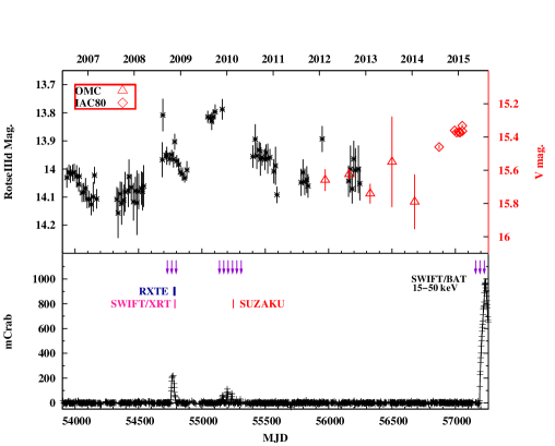
Figure 1: Comparison of the Swift/BAT light curve (15-50 keV) with the optical magnitudes (ROTSE, OMC, IAC80) of V 0332+53 since 2006. The BAT, ROTSE and OMC data points have been rebinned for clarity. The violet arrows in the X-ray panel represent the times of the periastron passages of the NS.

2.2 Optical spectroscopic observations

Optical spectroscopic observations of the donor star were performed since 26 September 2006 until 22 November 2014 (see on-line material Tab.2) with three different telescopes: the Russian-Turkish 1.5 m telescope (RTT150) at the TUG, the 2.56 m Nordic Optical Telescope (NOT) located at the Observatorio del Roque de los Muchachos (La Palma, Spain), and the 1.5 m Telescope at the Observatorio de Sierra Nevada (OSN-CSIC) in Granada (Spain).

The spectroscopic data from RTT150 were obtained with the TÜBİTAK Faint Object Spectrometer and Camera (TFOSC). The reduction of the spectra was done using the Long-Slit package of MIDAS. The low-resolution OSN spectra were acquired using Albireo spectrograph whereas the NOT spectra were obtained with the Andalucía Faint Object Spectrograph and Camera (ALFOSC). The reduction of this data set was performed using standard procedures within IRAF (Camero et al. 2014, for further details on the instrumentation and data reduction).

All spectroscopic data were normalized with a spline fit to continuum and corrected to the barycenter after the wavelength calibration. The full width at half maximum (FWHM) and equivalent width (EW) measurements of H_α lines were acquired by fitting Gaussian functions to the emission profiles using the ALICE subroutine of MIDAS.

Table 1: Log of the X-ray observations ¹.

Obs.	Date 2	MJD	Telescope	Exp.	Pulse
				time	period
				(s)	(s)
1	04/11/08	54774.636	RXTE 3	1 600	4.3742(1)
2	07/11/08	54777.999	RXTE	752	–
3	09/11/08	54779.731	RXTE	496	–
4	10/11/08	54780.594	RXTE	864	–
5	12/11/08	54782.394	RXTE	1 456	4.3740(1)
6	14/11/08	54784.511	RXTE	1 552	4.3746(6)
7	16/11/08	54786.543	RXTE	1 488	4.37450(2)
8	19/11/08	54789.826	RXTE	3 840	4.37540(2)
9	20/11/08	54790.775	RXTE	2 848	4.3763(1)
10	21/11/08	54791.743	RXTE	1 152	4.3760(1)
11	22/11/08	54792.270	RXTE	3 716	4.37610(4)
12	23/11/08	54793.273	RXTE	1 597	4.37620(4)
13	23/11/08	54793.387	RXTE	3 235	4.37620(5)
(5)	12/11/08	54782.384	Swift 4	1 706	–
(6)	14/11/08	54784.520	Swift	2 108	–
(7)	16/11/08	54786.533	Swift	2 307	–
(8)	19/11/08	54789.338	Swift	1 613	–
(9)	20/11/08	54790.811	Swift	1 597	–
(10)	21/11/08	54791.487	Swift	1 489	–
14	16/02/10	55243.264	Suzaku 5	15 946	4.37(1)
1 Standard mode for RXTE and Suzaku and Windowing
mode for Swift-XRT.
2 Observation date in the format (dd/mm/(20)yy).
3 RXTE/PCA exposure time.
4 Swift/XRT exposure time.
5 Suzaku/XIS1 exposure time.

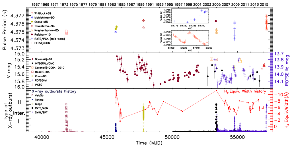
Figure 2: Top. Long-term pulse period history of V 0332+53 since its discovery in 1973. Middle. Long-term optical lightcurve of V 0332+53. All but the IAC80 light curve have been rebinned for clarity. Bottom. Type of X-ray outburst underwent by V 0332+53 (i.e. Type II, Intermediate, and Type I). The intensities are the same for outbursts of the same type, not having been corrected for the different energy bands. We only intend to be illustrative of the times and types of events. The long-term evolution of the H_α EW (red filled circles) is also overplotted. The measurements have been extracted from Iye & Kodaira (1985), Kodaira et al. (1985), Corbet et al. (1986), Negueruela et al. (1999), Masetti et al. (2005), Kiziloglu et al. (2008), Goranskij et al. (2010) and the present work.

2.3 X-ray Observations

The XRT (on-board the Swift satellite; Gehrels et al. 2004) observed V 0332+53 in Windowing Timing (WT) mode (1.7 ms time resolution, 1D Image) six times from 12 to 21 November 2008. Tab. 1 shows a summary of the log of these observations. To reduce the data and extract final products (spectra and light curves) we followed the standard recipe as detailed in the Swift/XRT data reduction guide. The relevant response matrix to use is given by the HEASARC’s calibration database (CALDB). All the XRT lightcurves were barycentred corrected. We also used for comparison data products supplied by the UK Swift Science Data Centre at the University of Leicester (Evans et al., 2009).

RXTE Proportional Counter Array (PCA; Jahoda et al. 1996) standard 1 and 2 data only from PCU-2 were selected for this work. To extract PCA products we followed the standard procedure showed in its cookbook. A systematic error of 0.5$\%$ was added in quadrature to the PCA standard 2 spectra, as recommended by the instrument team. Products from the High Energy X-ray Timing Experiment (HEXTE; Gruber et al. 1996) were also extracted using the corresponding cookbook recipe. Only standard mode data from cluster B were used. All the RXTE lightcurves were barycentred corrected.

In addition, we analysed one observation performed by Suzaku (Mitsuda et al., 2007) in 16 February 2010. We selected only data from the X-ray Imaging Spectrometer (XIS; Koyama et al. 2007) CCD and the PIN diode detector (10-70 keV) of the he Hard X-ray Detector (HXD; Takahashi et al. 2007). For this observation only XIS0, XIS1 and XIS3 detectors were available. Following the Suzaku ABC guide, we reprocessed all the data and extracted the final products. The clocking mode option was normal burst (1.0) with the 1/4 window selected (1 s time binning), and a data editing mode of 3${\times}$3. No pile-up correction was needed. The events were barycentred corrected.

We used the HEAsoft software version 6.15.1 (Arnaud, 1996) for the data analysis of all the instruments. Since 2008, the Gamma-ray Burst Monitor (GBM) on board the Fermi satellite, has been monitoring V 0332+53. In this work we used timing products provided by the GBM Pulsar Team (see e.g. Finger et al., 2009; Camero-Arranz et al., 2010, for a detailed description of the timing technique). We also used quick-look X-ray results provided by the RXTE All Sky Monitor team, and since 2008 we used the quick-look X-ray Swift/BAT transient monitor results provided by the Swift/BAT team (Krimm et al., 2013). See Fig. 2.

3 Results

3.1 Optical photometry

The optical light-curves of BQ Cam compared to the Swift/BAT data (15-50 keV) from June 2006 to June 2015 are shown in Fig. 1. In 2008, after being ${\approx}3.5$ yrs in quiescence in X-rays the system underwent a new active period. However the optical companion entered the brightening state nearly 1.5 yr before the NS. When the enhancement in the optical brightness reached a value of ${\approx}0.25$ mag. The X-ray outburst was triggered, around 17 October 2008 (MJD 54756) roughly six days before the periastron passage of the NS (vertical red-dashed lines in Fig. 1). This large flare lasted about 40 d and reached a flux of ${\approx}$214 mCrab within 3 weeks. It should be pointed out that the optical magnitude of V 0332+53 shows a sudden decrease when the X-ray outburst declines. Fading of the optical companion continued until the end of January 2009 (MJD ${\approx}$54850) and soon after it turned back to its brightening state. The X-ray flux, on the other hand, stayed at its quiescent level, until the Be star reached a peak value of ${\approx}$13.8 mag (ROTSE magnitude). A new X-ray phase of the system started in November 2009 again a few days after the periastron passage (MJD ${\approx}$55140) of the NS. That activity included five small but periodic outbursts separated by the orbital period (34.25 d) of the system classified as Type I.

The second outburst of these series was the most powerful one with a peak flux of ${\approx}$110 mCrab. The optical magnitude, on the other hand, started to decrease with declining of the second outburst (MJD ${\approx}$55201). The X-ray activities finished by the end of the May 2010 (MJD ${\approx}$55312) while the optical magnitude was still fading. It ceased around August 2011 (MJD ${\approx}$55780) and lasted ${\approx}$4 years. Our recent data from the IAC80 telescope and the optical camera OMC on board INTEGRAL, shows an optical enhancement of the counterpart BQ Cam, with the brightness varying from the quiescence level of ${\rm V}=15.93{\pm}0.55$ (06 Jan. 2012; MJD 55932.60) to ${\rm V}=15.332{\pm}0.008$ (1 Feb. 2015; MJD 57054.04; Camero-Arranz et al. 2015). This corresponds to an increment of ${\approx}0.6$ mag, similar to that observed during the brightening episodes occurred e.g. in 1983 (see Goranskij 2001) and in 2004 (Goranskij & Barsukova, 2004), but higher than the ones in 2008 (Kaur et al., 2008) and 2009 (Goranskij et al., 2010). This is confirmed by our only IR measurement from December 2014 (MJD 57011.869), that showed an unusually bright Be companion. The magnitudes obtained were J=11.228$\pm$0.003 mag, H=10.651$\pm$0.003 mag, and ${\rm K}_{\rm s}$=10.285$\pm$0.004 mag, which are comparable to those from December 1983 (Williams et al., 1983). We note that BQ Cam did not reach its maximum level (${\rm V}=15.2$ mag) in our observations from February 2015. The maximum has been probably reached recently, since the BAT monitor is currently detecting X-ray activity from V 0332+53 with a daily average flux of the order of 310.4 mCrab on 25 June 2015 (MJD 57198.0).

3.2 ${\rm H}_{\alpha}$ line

The long-term ${\rm H}_{\alpha}$ line monitoring of BQ Cam from September 2006 to November 2014 has been studied (see Fig. 3). In contrast to the previous works stating the ${\rm H}_{\alpha}$ profile variations (Negueruela et al., 1998, 1999), we did not see such variability patterns during the observation period. Instead, all the line profiles are nearly-symmetric in a single-peaked form despite the lack of the observations for the period 2010-2011.

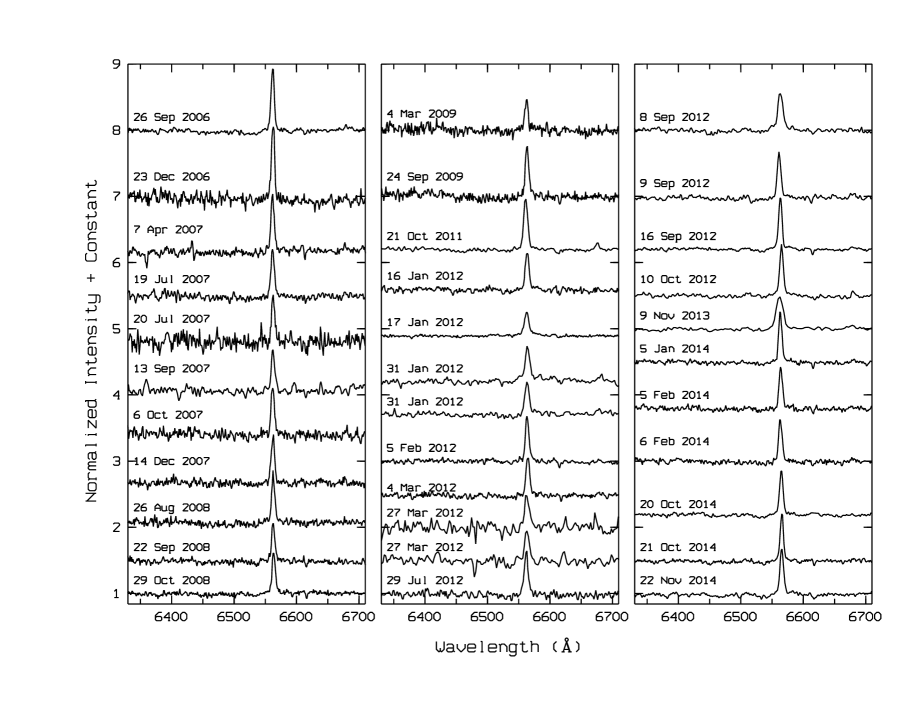
Figure 3: ${\rm H}_{\alpha}$ profiles of V 0332+53 selected between 2006 and 2014. The single-peaked emission of the line does not change on a long-term basis.

In spite of having the same single-peaked emission profile on a long-term basis, the ${\rm H}_{\alpha}$ line strength does not show a constant trend during the spectroscopic observations (see on-line material Tab. 2). In Fig. 4 the evolution of EW and FWHM measurements of the emission line are shown. The first two measurements of the line coincide with the declining phase of the optical outburst seen in the time interval MJD 53576-54180. The EW values decreased as the star faded away which can be attributed to the weakening of the decretion disc. Besides, this decreasing pattern continues after the optical outburst triggered (MJD 54324). Although our data coverage is not uniform, we see a reverse relation between the optical magnitude and the width of the emission line until 4 March 2009 (MJD 54894) when the lowest value of the EW of ${\rm H}_{\alpha}$ is reached (see Fig. 2). After about seven months, the EW reached a value of -5.21 Å. Although this sudden increase in the line width well fits with the rising of the optical magnitude, we cannot make any further explanation regarding the behavior of the emission line due to the lack of data for 2010-2011. In 2012-2014, we see that the strength of the ${\rm H}_{\alpha}$ line kept its varying pattern without a noticeable change in the optical magnitude indicating the upcoming mass ejection event.

In contrast to the variations in EW values, the FWHM values stayed approximately constant until the end of 2012. At that point, the FWHM values started to follow nearly the same pattern of EW. Indeed, showing a similar behavior is not unusual for EW and FWHM, since the width of the emission profile is directly related to the rotational velocity of the Be star. Hanuschik (1989) gives the relation between the ${\rm H}_{\alpha}$ widths and the projected rotational velocity, $v{\sin(i)}$. The projected rotational velocity of V 0332+53 is found to be $v{\sin(i)}=166.68\,{\rm km}\,{\rm s}^{-1}$, using the average values of -5.04 Å (i.e. $230\,{\rm km}\,{\rm s}^{-1}$) and 7.3 Å ($333.56\,{\rm km}\,{\rm s}^{-1}$) for the EW and FWHM, respectively (see on-line material Tab. 2). For the true rotational velocity of V 0332+53, we have assumed the inclination angle of the system of ${\rm i}{\leq}18.9^{\circ}$ as suggested by Zhang et al. (2005). Therefore, the lower limit to the true rotational velocity would be $514\,{\rm km}\,{\rm s}^{-1}$. Using the typical mass and radius values for a late O-type star (${\rm M}{\gtrsim}20\,{\rm M}_{\odot}$ and ${\rm R}{\gtrsim}15\,{\rm R}_{\odot}$), the break-up velocity is determined as $600\,{\rm km}\,{\rm s}^{-1}$ that is close to the rotational velocity.

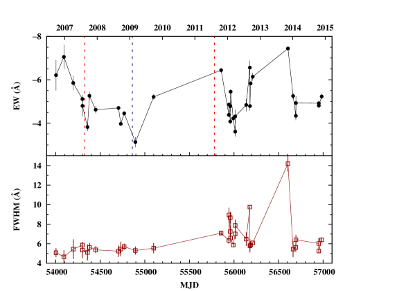
Figure 4: Evolution since 2006 of the EW and FWHM measurements of the ${\rm H}_{\alpha}$ emission line. The red-dashed vertical line denotes the beginning and the end of the optical outburst seen in ROTSEIIId light curve (see also Fig. 1) whereas the black-dashed line shows the time of the turning point from decreasing to increasing trend just after (${\approx}10$ d) the strong X-ray outburst around MJD${\approx}$54850.

3.3 X-ray activity

3.3.1 Periodic timing analysis

To search for periodic pulsations from the compact object we have used the tool efsearch from the Xronos package. This tool searches for periodicities in a time series by folding the data over a range of periods and by searching for a maximum chi-square as a function of period. Standard 1 PCA, XRT and Suzaku-XIS barycentred lightcurves for V 0332+53 were selected for this task (see Tab. 1). The resulted pulse periods can be seen in Fig. 2 and Tab. 1. The error on the measured spin periods is calculated using the chi-square versus spin period plot provided by efsearch. The points near the peak of this plot are fitted with a gaussian. The error on the gaussian centre estimate is taken as the error on the spin period. From Tab. 1 we can see that during the 2008 outburst decay the neutron star seems to spin slower, as expected. Additionally, we note that in Fig. 2 we do not include the pulse period obtained with Suzaku-XIS (${\rm P}_{pulse}=$4.37(1) s) because of its large uncertainty. Furthermore, we do not include any pulse period from the XRT data because they were not significantly detected.

3.3.2 Aperiodic timing analysis

We performed an analysis of the fast time variability of V 0332+53 in the 2-60 keV energy range of Obs. 1, 2, 6, 8 and 9. The net PCA count rate is ${\approx}700,600,300,300,160\,{\rm cts}\,{\rm s}^{-1}$ for Obs. 1-9, respectively. The rest of the observations either are too short and/or the source is too faint to perform timing analysis. The time resolution of the PCA in the mode used is 0.125 s.

We used the GHATS package, developed under the IDL environment at INAF-OAB, to produce the Power Density Spectra (PDS) from 512 points in each light curve. The PDS were then averaged together for each observation. The PCA light curve was binned at its time resolution (0.125 s). This yields a Nyquist frequency of $=4$ Hz. The PDS were normalized according to Leahy et al. (1983). All of the PDS show low-frequency band-limited noise (that may turn into peaked noise) and QPO noise.

PDS fitting was carried out with the standard XSPEC fitting package by using a unit response. Fitting the (2-60 keV) PDS with a model constituted by a zero centred Lorentzian for the flat-topped noise (hereafter called ${\rm L}_{1}$) plus a constant for the Poissonian noise (i.e. well reproduced by a powerlaw model component with its photon index frozen to zero in the fits) results in mostly acceptable chi-square values only for the PDS of Obs. 1, (see Tab. 2). In the case of Obs. 8, 9 the fit statistics with this model is worse and leaves some visible residuals, i.e. ${\chi}^{2}/{\nu}=290/252,233/252$, respectively. The fit to these observations improved by adding a further Lorentzian component (${\rm L}_{2}$) centred at ${\nu}=30-80\,$mHz. This component changed the (F-test) fits statistics by ${\Delta}{\chi}^{2}{\approx}20-30$ for ${\nu}=249$ d.o.f., thus a ${\leq}3{\sigma}$ improvement. For Obs. 2, 6 we took into account the latter feature only, since it is broad and therefore constitute a main part of the measure of the rms, i.e. by $(10-20)\%$. This resulted in a fit statistics of ${\chi}^{2}/{\nu}=253/252,255/252$ for Obs. 2, 6, respectively.

The fit of the (2-60 keV) PDS with a model constituted by a zero (${\rm L}_{1}$) and a ${\nu}=30-80\,$mHz (${\rm L}_{2}$) centred Lorentzians (${\rm L}_{2}$ only for Obs. 2 and 6) for the band-limited noise plus a constant for the Poissonian noise results in a poor description of the data for Obs. 6, 8, 9. The fit statistics with this model is of ${\chi}^{2}/{\nu}=255/252,263/249,209/249$ for Obs. 6-9, respectively. In these observations there are positive residuals centred in the range of $(220-240)$ mHz that we fitted by adding a further Lorentzian component (${\rm L}_{\rm QPO}$) centred at those frequencies. This component changed the fits statistics by ${\Delta}{\chi}^{2}{\approx}12,19,13$ for ${\nu}=249,246,246$ d.o.f., thus a $(2.9,3.9,3.0){\sigma}$ improvement for Obs. 6-9, respectively. We took into account this feature, since it is broad and therefore affects substantially the measure of the rms, i.e. by ${\approx}(2-4)\%$ for all the observations. These positive features have a peaked form, thus we will call them ${\rm QPOs}$, consistently with previous findings (Qu et al., 2005; Reig, 2008; Reig & Nespoli, 2013). The detection of this peak is only significant for Obs. 8, which can be explained since this is the observation with the longest exposure time of the sample.

We calculated the fractional rms from the best fit model (integrated in the $(8{\times}10^{-3}-4)$ Hz band). This was found to be $(15-20)\%$ in the 2–60 keV energy range. The results obtained from the global fits (i.e. using the lorentz+lorentz+lorentz+powerlaw model in XSPEC) are reported in Tab. 2. We plot in Fig. 5 the broad-band PDS with the best-fit model. We notice that our results are broadly in agreement with those previously obtained (Reig & Nespoli, 2013).

Table 2: Results from the RXTE timing analysis¹.

	Obs. 1	Obs. 2	Obs. 6	Obs. 8	Obs. 9
${\nu}_{\rm 1}$	$7.5{\pm}7$	–	–	$10{\pm}8$	$12{\pm}10$
FWHM	$174{\pm}14$	–	–	$29{\pm}14$	$22{\pm}20$
Norm.	$21.7{\pm}1.2$	–	–	$1.7{\pm}0.8$	$1.1{\pm}0.6$
rms ($\%$)	$16.4{\pm}0.4$	–	–	$6.2{\pm}0.3$	$8.3{\pm}0.6$
${\nu}_{\rm 2}$	–	$48{\pm}13$	$36{\pm}11$	$82{\pm}19$	$77{\pm}25$
FWHM	–	$147{\pm}15$	$166{\pm}12$	$137{\pm}25$	$160{\pm}24$
Norm.	–	$17.2{\pm}1.5$	$9.1{\pm}0.5$	$1.3{\pm}0.4$	$1.3{\pm}0.4$
rms ($\%$)	–	$16.4{\pm}0.7$	$16.5{\pm}0.5$	$6.5{\pm}0.3$	$8.4{\pm}0.6$
${\nu}_{\rm QPO}$	–	–	$231{\pm}5$	$226{\pm}8$	$233{\pm}4$
FWHM	–	–	$16{\pm}11$	$33{\pm}18$	$17{\pm}16$
Norm.	–	–	$0.46{\pm}0.15$	$0.16{\pm}0.06$	$0.12{\pm}0.04$
rms ($\%$)	–	–	$3.8{\pm}2.1$	$2.3{\pm}1.0$	$2.7{\pm}1.8$
${\Gamma}_{\rm poisson}$	$0$	$0$	$0$	$0$	$0$
${\rm N}_{\rm poisson}$	$1.84{\pm}0.04$	$1.59{\pm}0.05$	$1.79{\pm}0.03$	$1.90{\pm}0.03$	$1.93{\pm}0.03$
${\chi}^{2}/{\nu}$	$0.84\,(213/252)$	$1.0\,(253/252)$	$0.98\,(243/249)$	$0.99\,(244/246)$	$0.80\,(196/246)$
1 Model used: lorentz+lorentz+lorentz+powerlaw for five RXTE/PCA observations.
2 The PDS were created in the (2–60) keV energy band and $(8{\times}10^{-3}-4)$ Hz frequency range.
3 The frequency and width (${\nu}$ and FWHM) of the components are shown in units of mHz.
4 Errors are $68\%$ confidence errors.

Figure 5: Power density spectra of the RXTE PCA data in the energy and frequency range (2-60 keV) and 0.008-4 Hz, respectively, during observations 1, 2, 6, 8 and 9 (top-left to bottom-right) with the best fit model (solid line) and the model components (dotted line). The results of the fitting are shown in Tab. 2 and discussed in the text.

3.3.3 Spectral analysis

We fitted the brightest background-subtracted spectra with standard spectral models in XSPEC 12.8.2 (Arnaud, 1996). All errors quoted in this work are $68\%$ ($1{\sigma}$) confidence. The spectral fits were limited to the 1-10, 4.5-28, 26-60 keV range for the XRT, PCA and the HEXTE, respectively, where the calibration of the instruments is the best. The spectra were grouped in order to have at least 100, 50, 50 counts for the XRT, PCA and HEXTE, respectively for each background-subtracted spectral channel and to avoid oversampling of the intrinsic energy resolution.

As it is a common procedure in observational studies of NS systems we used empirical models to describe the X-ray spectra. To compare our results with previous studies we used the same (or very similar) spectral components. To fit the spectral continuum we used a model composed by photoelectric absorption (Balucinska-Church & McCammon 1992; phabs in XSPEC) and a power-law with a high-energy exponential cutoff (cutoffpl). The absorption component was not used in Obs. 1-4 and 11 (we did not fit the data from Obs. 12,13 because of the lack of counts), since PCA spectra are not affected (i.e. at ${\rm E}{\geq}4.5$ keV). In the case of XRT observations, with lower energy coverage (i.e. at ${\rm E}{\geq}1$ keV) the absorption component was included in all our fits. This model provided significant wavy residuals in the whole spectra of all the observations with non acceptable chi-squared values (${\chi}^{2}$/${\nu}{\approx}5-60$; with ${\nu}$ being the number of degrees of freedom, i.e. d.o.f.).

Table 3: Results from the ${\it RXTE}$ spectral analysis only¹.

	Obs. 1	Obs. 2	Obs. 3	Obs. 4	Obs. 11
${\rm E(1)}_{\rm gabs}$	$7.6{\pm}2.8$	$8.0{\pm}2.3$	$9.0{\pm}0.5$	$6.5{\pm}0.7$	$5{\pm}2$
${\sigma}{\rm(1)}$	$4.6{\pm}1.6$	$4.1{\pm}0.8$	$3.3{\pm}0.6$	$6{\pm}5$	$7{\pm}3$
${\rm S(1)}$	$15{\pm}8$	$9{\pm}7$	$2.2{\pm}0.9$	$70{\pm}40$	$11{\pm}10$
${\rm E(2)}_{\rm gabs}$	$31.6{\pm}0.7$	$31.3{\pm}0.8$	$31.8{\pm}0.8$	$29.7{\pm}1.2$	$28.4{\pm}1.0$
${\sigma}{\rm(2)}$	$4.3{\pm}0.4$	$4.6{\pm}0.4$	$5.0{\pm}0.6$	$4.1{\pm}0.8$	$3.4{\pm}0.5$
${\rm S(2)}$	$17{\pm}3$	$20{\pm}4$	$23{\pm}5$	$14{\pm}6$	$8{\pm}3$
${\rm E}_{\rm gauss}$	$6.3{\pm}0.5$	$6.40{\pm}0.10$	$6.9{\pm}1.5$	$6.3{\pm}0.6$	$5.7{\pm}0.6$
${\sigma}$	$0.18{\pm}0.20$	$0.22{\pm}0.20$	$1.6{\pm}0.5$	$0.5{\pm}0.4$	$1.1{\pm}0.6$
${\rm N}$	$0.012{\pm}0.005$	$0.009{\pm}0.004$	–	$0.014{\pm}0.010$	$0.02{\pm}0.01$
${\Gamma}_{\rm pow}$	$-0.7{\pm}0.5$	$-0.51{\pm}0.24$	$-0.93{\pm}0.28$	$-0.7{\pm}0.5$	$-0.7{\pm}0.3$
${\rm E}_{\rm cutoff}$	$5.7{\pm}0.6$	$6.6{\pm}0.5$	$5.7{\pm}0.6$	$5.0{\pm}0.8$	$5.68{\pm}0.15$
${\rm F}_{\rm X}$	$10{\pm}4$	$8{\pm}4$	$4.7{\pm}0.1$	$4.5{\pm}0.3$	$1.3{\pm}0.7$
${\rm L}_{\rm X}$	$5.9{\pm}2.4$	$4.7{\pm}2.4$	$2.8{\pm}0.3$	$2.7{\pm}0.3$	$0.8{\pm}0.4$
${\rm C}_{\rm PCA}$	$1$	$1$	$1$	$1$	$1$
${\rm C}_{\rm HEXTE}$	$0.50{\pm}0.05$	$0.45{\pm}0.07$	$1.3{\pm}0.3$	$1.5{\pm}0.3$	$0.40{\pm}0.07$
${\chi}^{2}$/${\nu}$	$0.83\,(43/52)$	$0.90\,(47/52)$	$1.1\,(56/52)$	$1.2\,(64/52)$	$1.1\,(56/52)$
1 Model used: constant${\times}$gabs${\times}$gabs( cutoffpl + gaussian ) for the 4.5-60 keV RXTE
spectra.
2 Centroid, line-width of the lines, normalization of the gaussian line, flux and luminosity
in units of ${\rm keV}$, ${\rm cm}^{-2}\,{\rm s}^{-1}$, $10^{-9}\,{\rm erg}\,{\rm s}^{-1}\,{\rm cm}^{-2}$ and $10^{37}\,{\rm erg}\,{\rm s}^{-1}$, respectively.
3 Errors are $68\%$ confidence errors.

Table 4: Results from the ${\it Swift}$ $+$ RXTE spectral analysis¹.

	Obs. 5	Obs. 6	Obs. 7	Obs. 8	Obs. 9	Obs. 10
${\rm N}_{\rm H}$ $({\times}10^{22})\,({\rm cm}^{-2})$	$1.01{\pm}0.08$	$0.74{\pm}0.07$	$0.84{\pm}0.07$	$0.80{\pm}0.13$	$0.77{\pm}0.07$	$0.93{\pm}0.12$
${\rm E(1)}_{\rm gabs}$ (${\rm keV}$)	$4.1{\pm}1.6$	$7.8{\pm}0.7$	$8.5{\pm}0.5$	$7.0{\pm}1.0$	$7.2{\pm}0.6$	$8.86{\pm}0.20$
${\sigma}{\rm(1)}$ (${\rm keV}$)	$6.6_{-0.5}^{+1.7}$	$4.3{\pm}0.7$	$3.0{\pm}0.8$	$5.1{\pm}1.4$	$5.5{\pm}0.6$	$7{\pm}3$
${\rm Strength(1)}$	$18_{-5}^{+13}$	$12{\pm}4$	$1.9_{-0.4}^{+1.7}$	$28{\pm}14$	$15{\pm}5$	$60{\pm}30$
${\rm E(2)}_{\rm gabs}$ (${\rm keV}$)	$30.8{\pm}0.8$	$29.3{\pm}1.1$	$26.8{\pm}0.9$	$30.0{\pm}1.4$	$30.0{\pm}2.0$	$27.5{\pm}2.3$
${\sigma}{\rm(2)}$ (${\rm keV}$)	$4.7{\pm}0.5$	$3.4{\pm}0.4$	$2.7{\pm}0.5$	$4.0{\pm}0.7$	$3.5{\pm}0.5$	$2.15{\pm}1.0$
${\rm Strength(2)}$	$19{\pm}4$	$14{\pm}4$	$6.0{\pm}2.0$	$12{\pm}4$	$16{\pm}9$	$10{\pm}8$
${\rm E}_{\rm gauss}$ (${\rm keV}$)	$6.56{\pm}0.16$	$6.23{\pm}0.20$	$6.23{\pm}0.19$	$6.15{\pm}0.4$	$6.5{\pm}0.5$	$6.5{\pm}0.8$
${\sigma}$ (${\rm keV}$)	$0.004_{-0.003}^{+0.23}$	$0.4{\pm}0.3$	$0.34{\pm}0.20$	$1.25{\pm}0.25$	$0.003{\pm}0.003$	$1.4{\pm}0.9$
${\rm N}$ (${\rm cm}^{-2}\,{\rm s}^{-1}$)	$0.55{\pm}0.10$	$0.007{\pm}0.004$	$0.0013{\pm}0.0010$	$0.05{\pm}0.04$	$0.0012{\pm}0.0007$	$0.07{\pm}0.05$
${\Gamma}_{\rm pow.}$	$-0.02{\pm}0.21$	$-0.27{\pm}0.12$	$0.05{\pm}0.10$	$-0.20{\pm}0.20$	$-0.49{\pm}0.10$	$0.0{\pm}0.4$
${\rm E}_{\rm cutoff}$ (${\rm keV}$)	$5.4{\pm}0.4$	$5.8{\pm}0.7$	$10.3{\pm}1.6$	$6.0{\pm}0.5$	$5.2{\pm}0.7$	$7{\pm}4$
${\rm F}_{\rm X}$ 1 (${\times}10^{-9}$ ${\rm erg}\,{\rm s}^{-1}\,{\rm cm}^{-2}$)	$4.3{\pm}0.4$	$6.5{\pm}0.6$	$6.3{\pm}0.6$	$6.2{\pm}0.6$	$3.3{\pm}0.3$	$3.2{\pm}0.3$
${\rm L}_{\rm X}$ (${\times}10^{37}$ ${\rm erg}\,{\rm s}^{-1}$)	$2.5{\pm}0.3$	$3.8{\pm}0.4$	$3.8{\pm}0.4$	$3.7{\pm}0.4$	$2.0{\pm}0.2$	$1.9{\pm}0.3$
${\rm C}_{\rm PCA}$	$1$	$1$	$1$	$1$	$1$	$1$
${\rm C}_{\rm HEXTE}$	$1.43{\pm}0.20$	$0.45{\pm}0.15$	$0.11{\pm}0.05$	$0.33{\pm}0.06$	$0.61{\pm}0.15$	$0.26{\pm}0.17$
${\rm C}_{\rm XRT}$	$0.87{\pm}0.08$	$0.39{\pm}0.03$	$0.39{\pm}0.03$	$0.29{\pm}0.03$	$0.41{\pm}0.03$	$0.48{\pm}0.05$
${\chi}^{2}$/${\nu}$	$0.93\,(182/195)$	$0.97\,(152/156)$	$1.13\,(183/161)$	$0.87\,(97/112)$	$0.94\,(97/103)$	$1.02\,(99/97)$
1 Model used: phabs${\times}$constant${\times}$gabs${\times}$gabs( cutoffpl + gaussian ) for the 1-60 keV Swift $+$ RXTE spectra.
2 Errors are $68\%$ confidence errors.

The fits and the residuals of the whole spectra improved (${\chi}^{2}$/${\nu}{\approx}1.5-6$) by the addition of a cyclotron line scattering feature (CRSF; hereafter referred to as “cyclotron feature”). It was accounted for with a gaussian absorption line (gabs). The use of this model component and/or the obtained line parameters are consistent with previous studies (Kreykenbohm et al., 2005; Tsygankov et al., 2006; Reig et al., 2006; Reig & Nespoli, 2013; Lutovinov et al., 2015). The parameters were let to be free in the HEXTE data and tied to those in the XRT and PCA data.

The fits still show significant residuals at 7-10 keV. This feature is known as the “10 keV feature”, and its origin is uncertain (Coburn et al., 2002). We modeled it as a gaussian absorption line (gabs), thus improving the fits substantially (${\chi}^{2}$/${\nu}{\approx}1.0-1.2$). In this case the parameters were let to be free in the PCA data and tied to those in the XRT and HEXTE data. The values obtained are within those expected (Coburn et al., 2002) but with broader dispersion than those obtained e.g. for XTE J1946+274 by Müller et al. (2012).

Although the beneath of the spectral fits, there are still peaked positive residuals in the region 6-7 keV of the PCA spectra. We accounted for them adding a gaussian line profile (gaussian) at 6.4-6.97 keV in order to account for the Fe K_α fluorescence line. The PCA residuals flattened and we obtained the final fitting solution in this way.

To account for uncertainties in the absolute flux normalization between PCA and HEXTE we introduced a multiplicative constant that was fixed to 1 for the PCA and let to vary freely for HEXTE. In the case of XRT, PCA and HEXTE data we fixed the multiplicative constant of PCA to 1 and the rest to vary freely. The most relevant results of this spectral analysis and the derived unabsorbed fluxes and luminosities are shown in Tab. 3,4 and in Fig. 6.

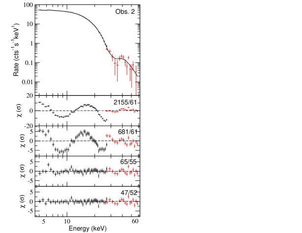
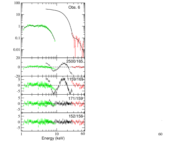
Figure 6: The two (upper) panels (left and right) show two example spectra of V 0332+53. Obs. 2 is one of the two observations with the highest count rates while Obs. 6 is the dataset with the highest count rate with all the instruments available (black, red and green correspond to PCA, HEXTE and XRT, respectively). The (lower) panels show the behaviour of the residuals when adding the different components one by one. Number at the right of each panel indicate the best fit statistics (${\chi}^{2}$/d.o.f.). From upper to lower panels: 1) best-fit using the cutoffpl model component only (i.e. continuum model); 2) residuals after adding the ${\approx}10$ keV (absorption) feature to the continuum model; 3) residuals after adding the cyclotron feature; 4) residuals after adding the Fe ${\rm K}_{\alpha}$ line to the model (and final residuals of the model). Note that the same vertical axis is used in both panels.

In addition, we fitted the spectra obtained with Suzaku, during much a lower luminosity period (see Fig. 7 and Tab. 5). Spectra from XIS1, XIS3 and PIN were fitted in the 0.8-10,14-25 keV energy range, with the 1.6-2.3 keV energy range ignored due to the uncertainties in calibration associated with the instrumental Si K edge. The spectra were grouped to have at least 50,250 counts for the two XIS and PIN, respectively. In this case a model composed by photoelectric absorption (phabs) and a power-law with an exponential high-energy cutoff of the type “highecut” was a rather better description than “cutoffpl” (i.e. ${\Delta}\,{\chi}^{2}=15$ for the same number of d.o.f and better residuals). With this model we obtained a statistics of ${\chi}^{2}$/${\nu}=1.4$ and systematic residuals at ${\rm E}<4$ KeV, that we improved by adding a blackbody spectrum with normalization proportional to the surface area (bbodyrad), obtaining a fit statistics of (${\chi}^{2}$/${\nu}=1.3$ for the same number of d.o.f.). Because the normalization of the black-body component was not well constrained we tried to improve it and changed it by an emission component describing an accretion disc consisting of multiple blackbody components (diskbb; Mitsuda et al. 1984; Makishima et al. 1986). We obtained a very similar fit statistics (see Tab. 5). A plausible origin for the first model component (bbodyrad) is the NS surface or perhaps the boundary layer (if present). Low-level accretion onto the surface of a neutron star can indeed produce a black-body like spectrum (Zampieri et al., 1995). Still, a disc origin cannot be ruled out since it was also possible to fit the data with a multicolor disc blackbody. Similar results for a set of low-accreting NS have been recently obtained (Armas Padilla et al., 2013), but the temperatures found are ${\rm kT}{\approx}=0.5-0.7$ keV, thus much lower than in our case (${\rm kT}{\approx}=2.4{\pm}0.9$ keV). The higher value we obtain might be indicative of the much higher accretion rate in our case. Nevertheless, with the current data it is not possible to discern which model component is better to describe the data.

To account for the uncertainties in the absolute flux normalization between XIS1, XIS3 and PIN we introduced a multiplicative constant that was fixed to 1 for XIS1 and let to vary freely for XIS3 and PIN. The most relevant results of this spectral analysis and the derived unabsorbed fluxes and luminosities are shown in Tab. 5.

Table 5: Results from the ${\it Suzaku}$ spectral analysis¹.

	Obs. 14
${\rm N}_{\rm H}$ $({\times}10^{22})$ (${\rm cm}^{-2}$)	$1.2{\pm}0.1$
${\rm kT}_{\rm bb}$ (${\rm keV}$)	$2.4{\pm}0.9$
${\rm N}_{\rm bb}$	$0.011{\pm}0.007$
${\Gamma}_{\rm pow.}$	$-1.3{\pm}1.6$
${\rm E}_{\rm cutoff}$ (${\rm keV}$)	$15-190$
${\rm E}_{\rm f}$ (${\rm keV}$)	$1.0{\pm}1.0$
${\rm F}_{\rm X}$ (${\times}10^{-11}$) (${\rm erg}\,{\rm s}^{-1}\,{\rm cm}^{-2}$)	$2.4{\pm}0.9$
${\rm L}_{\rm X}$ (${\times}10^{35}$) $({\rm erg}\,{\rm s}^{-1})$	$1.4{\pm}0.5$
${\rm C}_{\rm XIS1}$	$1$
${\rm C}_{\rm XIS3}$	$1.35{\pm}0.04$
${\rm C}_{\rm PIN}$	$0.4{\pm}0.3$
${\chi}^{2}$/${\nu}$	$1.35\,(221/163)$
1 Model used: phabs${\times}$constant${\times}$highecut(diskbb +
powerlaw) for the 0.8-30 keV Suzaku spectrum.
2 Errors are $68\%$ confidence errors.

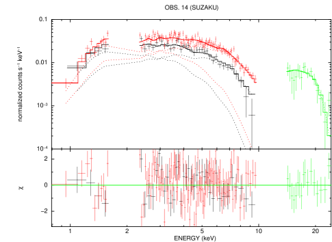
Figure 7: Energy spectrum from V 0332+53 during Obs. 14 with Suzaku (see Tab. 5 for the observation details and the results of the spectral analysis). Black, red and green correspond to XIS1, XIS3 and PIN, respectively.

4 Discussion

4.1 Long-term Be-disc/neutron star interaction

From the long-term observations of V 0332+53 we can see that V 0332+53 spends most of its time in the optical brightening phases (Fig 2). The most significant one is the period between 1993-2005. It started approx. 4 years after the giant outburst that the system exhibited in 1989 and peaked simultaneously with the X-ray maximum in 2004. Indeed all of the optical brightening episodes of BQ Cam are accompanied with the X-ray activities. It is important to note that the brightness of the optical companion decreases after the X-ray outbursts. This behavior can be well explained by the weakening of the decretion disc during the mass transfer to the NS.

Having a moderate eccentricity of ${\rm e}=0.31$ with a short orbital period of ${\rm P}_{\rm orb}=34.25$ d, V 0332+53 is one of the BeXBs for which the effect of the truncation exerted by the NS is likely to be observed. Due to the small orbit of the companion, the decretion disc cannot expand so much. Thus, it is truncated at a radius smaller than the critical Roche radius. Since the amount of the material supported by the Be star to the disc would be accumulated in time, the increase in the optical brightness can be understood in this way. However the accumulation of the material particularly at the outer part of the disc makes these regions to become optically thick. According to theory by either the radiation-driving warping or a global density wave the outer part of the disc is strongly elongated (Okazaki and Negueruela, 2001). In general, the existence of the global density waves in the decretion disc are observationally supported by the V$/$R variations seen in the emission line profiles. Although the line profile variations of V 0332+53 were previously observed (Negueruela et al., 1998) during the period 1990-1991, ${\rm H}_{\alpha}$ lines are always seen in nearly symmetric single-peaked emissions without any significant variations for the time interval 2006-2014. Therefore, we do not have any evidence to support the idea of the perturbations occurred in the disc as well as the V/R variations.

4.2 X-ray behaviour

4.2.1 Spectral evolution

From the RXTE and Swift observations reported in this work we see a decrease of the X-ray luminosity of V 0332+53 during the latest part of the intermediate-luminosity 2008 outburst. Assuming a 7 kpc distance (Negueruela et al., 1999), the luminosity gradually dropped from $\sim$6 to $\sim$1$\times 10^{37}$ erg s^-1 in the 5-60 keV energy range from Obs. 1-11. The luminosities are also in accordance with those obtained during the decay phase of the 2005 outburst (Mowlavi et al., 2006). Eventually, during the Suzaku observation (Obs. 14) we obtain the lowest luminosity ($\sim$1$\times 10^{35}$ erg s^-1).

A recent study of V 0332+53 during giant outbursts at different luminosities has provided crucial insights into the most frequent states of V 0332+53 (Reig & Nespoli, 2013). Their Fig. 2 shows the existence of two separate regimes (the high-luminosity diagonal branch and the low-luminosity horizontal branch). They are separated by a critical luminosity (${\rm L}_{\rm crit}{\approx}1-4{\times}10^{37}$ erg s^-1), which corresponds to the range of luminosities reported in our work during Obs. 1-11. Both regimes/states are clearly well-populated by X-ray observations whilst observations around the critical luminosity are scarce.

The spectral variability of V 0332+53 has been well studied by different authors, confirming the softening of V 0332+53 as the flux decreased. Baykal et al. (2007) suggested that this type of spectral softening with decreasing flux was mainly a consequence of mass accretion rate change. In particular, Reig et al. (2010) (and references therein) explained that increased mass accretion rates are expected to result in harder X-ray spectra due to Comptonization processes. In our work we see the same trend photon index versus flux.

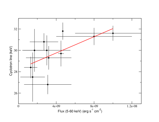
Figure 8: Flux in the 5-60 keV energy range versus the cyclotron line energy centre for Obs. 1-11. See on-line material Tab. 3 for the (not-rounded) list of values used.

The values previously obtained for the energy centre of the cyclotron line have shown a strong anti-correlation with luminosity in V 0332+53 (Tsygankov et al., 2006; Mowlavi et al., 2006; Tsygankov et al., 2010; Reig & Nespoli, 2013) during giant outbursts. Somehow weaker anti-correlation has been found in 4U 0115+63 (Mihara et al., 2004; Nakajima et al., 2006) and no correlation in 1A 0535+262 (Caballero et al., 2007). In our work a positive correlation of the line energy centre with luminosity is observed (see Fig. 8). The correlation coefficient of the fit is +0.64 (i.e. null two-tailed probability of 0.03). This kind of behaviour has also been observed in A 0535+262 during an intermediate-luminosity outburst (${\rm L}_{\rm X}=4{\times}10^{37}\,{\rm erg}\,{\rm s}^{-1}$; Sartore et al. 2015). We notice that previously Reig & Nespoli (2013) already pointed out for a tentative positive correlation for the latter source. This effect appears to be a natural consequence of accretion onto X-ray pulsars with the strongest magnetic fields in the sub-critical regime (Mushtukov et al., 2015). The values we have obtained for the width of the cyclotron line are all ${\approx}4$ keV, in contrast to the values obtained during high flux states (6-8 keV; Tsygankov et al. 2010) but in full agreement with those obtained in intermediate flux states (4 keV; Mowlavi et al. 2006).

4.2.2 Quasi Periodic Oscillations

We have found that the PDS of V 0332+53 during our observations are best described by band-limited noise plus QPO noise during the latest observations. The QPO noise consists of a component at a frequency of ${\approx}0.22-0.23$ Hz. This feature has also been reported in the 2-60 keV RXTE-PCA PDSs obtained during the 2004-2005 outburst decay (Qu et al., 2005). They found a QPO at ${\approx}$0.22 Hz in addition to a narrow peak (i.e. pulsation from the pulsar) close to that frequency (${\approx}$0.23 Hz). The QPO was detected when the luminosity was at a mid-flux or even lower flux level of the outburst. The rms strength of this QPO also amounts to a few per cent in that work. The 0.22 Hz QPO was observed around the spin frequency in both the INTEGRAL (Mowlavi et al., 2006) and RXTE data during the 2005 outburst decline (Qu et al., 2005; Reig et al., 2006). In addition, Takeshima et al. (1994) discovered another QPO with a centroid frequency of ${\approx}$0.05 Hz and a relative root mean square (rms) amplitude of ${\approx}$5%, in the 2.3-37.2 keV data from the 1989 outburst of V 0332+53. We do not find any signal of the QPO at ${\approx}$0.05 Hz although we find the presence of a broad component at around that frequency (that may turn eventually into peak noise, i.e. QPO). The QPO detected in V 0332+53 at ${\approx}$0.22 Hz constitutes the first detection of a QPO riding on the spin frequency of a NS and points out to a strong coupling between the periodic (i.e. the pulses) and the red-noise (i.e. broad band QPO signal) components (Qu et al., 2005).

The existence of a QPO signal with a similar frequency to the spin of the NS suggests that they are related somehow. One model to explain such coincidence was given by Lazzati & Stella (1997) and Burderi et al. (1997). They proposed that the QPO is originated in the magnetosphere around the NS. Additionally, they argued that the accretion flow is inhomogeneous near the surface of the NS, and that random shots are characterized by an arbitrary degree of modulation. The combination of rotation and radiative transfer effects should therefore produce a periodic modulation of the shots similar to that of any continuum X-ray emission from the polar caps. They proposed that a coupling between the periodic and red-noise variability should be frequently present in X-ray pulsars.

In our case and in contrast to previous observations during giant flares (Reig et al., 2006; Reig, 2008) the QPO signal appears during the lowest of the measured fluxes (${\rm L}_{\rm X}{\leq}4{\times}10^{37}$ ${\rm erg}\,{\rm s}^{-1}$). If the QPO has an origin on the magnetosphere of the NS (and is not an artifact from our observations), it should be “more visible” when the accretion column is more tenuous (or even absent). Summarizing, it looks like that during our latest Obs. 6-11 we might be witnessing the innermost parts closest to the magnetosphere surroundings.

5 Summary and conclusions

In this paper we present a multi-wavelength study of the Be/X-ray binary system V 0332+53 with the main goal of studying its transient behavior during its intermediate luminosity X-ray outburst in 2008. After being ${\approx}3.5$ yr in quiescence in X-rays the system underwent a new active period. A new X-ray outburst was detected around 17 October 2008, roughly six days before the periastron passage of the NS. We note that the optical companion entered the brightening state nearly 1.5 yr before the X-ray outburst.

V 0332+53 was in quiescence until the optical magnitude approached a peak value of ${\rm V}=15.2$ mag. at the end of 2009, indicating the beginning of another mass ejection event. In November 2009 a series of five small Type I periodic outbursts was observed. The X-ray activities finished by the end of May 2010 whist the optical magnitude was still fading. It ceased around August 2011 for about ${\approx}3.5$ yr. Our recent data showed that a mass ejection event is currently taking place, exhibiting an increase of ${\approx}0.6$ in the V mag. It probably started around 2013 and peaked in June 2015 when a new (type II) X-ray outburst was detected. This is similar to those observed during the brightening episodes occurred e.g. in 1983 and in 2004, but higher than the ones in 2008 and 2009. Our only IR measurement from December 2014 also showed an unusually bright Be companion.

The broad-band 1-60 keV X-ray spectra of the NS during the decay of the 2008 outburst were all well fitted with the standard cutoffpl phenomenological model, enhanced by a narrow iron ${\rm K}_{\alpha}$ fluorescence line at 6.4 keV together with a cyclotron line scattering feature at ${\approx}30$ keV. Our study confirms the softening of V 0332+53 as the flux decreased. During our lowest flux observation made with Suzaku (${\rm L}_{\rm X}=10^{35}\,{\rm erg}\,{\rm s}^{-1}$) on 2010, compatible with V 0332+53 being at a level slightly above from quiescence, we detected a very soft spectrum that could be well described by adding a (single or multiple) soft black-body component(s).

We tentatively see an increase of the cyclotron line energy with increasing flux. If confirmed (with better observations) this might constitute the first detection of such positive correlation of the cyclotron line energy versus luminosity in V 0332+53. Regarding the fast aperiodic timing properties, we detect a QPO at $227{\pm}9$ mHz during the lowest luminosities. The latter might indicate that the inner regions surrounding the magnetosphere are more visible during the lowest flux stages. Due to their low significance we advice that longer and better observations with current (and/or future) X-ray satellites are needed in order to confirm/discard these results.

Acknowledgments. We thank the anonymous referee and S. Campana for helpful comments. We also thank K. Page and the Swift team at Leicester (UK), A. J. Castro-Tirado (on behalf of the BOOTES collaboration), I. E. Papadakis and J. Garcia-Rojas for helpful discussions/insights and/or for making part of these observations possible. RH acknowledges GA CR grant 13-33324S. MCG acknowledges support by the European social fund within the framework of realizing the project “Support of inter-sectoral mobility and quality enhancement of research teams at Czech Technical University in Prague”, CZ.1.07/2.3.00/30.0034. This research has made use of the General High-energy Aperiodic Timing Software (GHATS) package developed by T.M. Belloni at INAF - Osservatorio Astronomico di Brera.

Table 1: ON-LINE MATERIAL. Optical photometric observations from the IAC80 telescope.

MJD	V	error	B	error
56871.2368550198	15.460	0.013	17.037	0.071
56993.9640124198	15.360	0.006	16.919	0.021
57009.0723979599	15.373	0.005	17.006	0.013
57026.9773657001	15.372	0.008	16.945	0.031
57036.8705536202	15.373	0.005	16.967	0.013
57054.0418117600	15.332	0.008	16.853	0.031
57054.8470330602	15.364	0.006	16.955	0.024

Table 2: ON-LINE MATERIAL. ${\rm H}_{\alpha}$ line EW and FWHM measurements of V 0332+53. Negative values of EW indicate that the line is in emission.

DATE	MJD	EW	FWHM	Telescope
		(Å)	(Å)
26-Sep-2006	54004.9238	$-$6.21$\pm$0.71	6.18$\pm$0.38	RTT150
23-Dec-2006	54092.9543	$-$7.05$\pm$0.56	5.83$\pm$0.55	RTT150
07-Apr-2007	54197.7388	$-$5.85$\pm$0.33	6.48$\pm$0.83	RTT150
19-Jul-2007	54300.0279	$-$5.11$\pm$0.10	6.83$\pm$0.22	RTT150
20-Jul-2007	54301.0591	$-$4.80$\pm$0.49	6.40$\pm$0.68	RTT150
13-Sep-2007	54356.9962	$-$3.82$\pm$0.18	6.20$\pm$0.67	RTT150
06-Oct-2007	54379.0510	$-$5.26$\pm$0.18	6.62$\pm$0.40	RTT150
14-Dec-2007	54448.8768	$-$4.62$\pm$0.17	6.42$\pm$0.29	RTT150
26-Aug-2008	54704.9757	$-$4.70$\pm$0.09	6.31$\pm$0.48	RTT150
22-Sep-2008	54731.0652	$-$3.97$\pm$0.09	6.49$\pm$0.62	RTT150
29-Oct-2008	54768.8500	$-$4.45$\pm$0.10	6.69$\pm$0.26	RTT150
04-Mar-2009	54894.7260	$-$3.13$\pm$0.23	6.36$\pm$0.34	RTT150
24-Sep-2009	55098.9814	$-$5.21$\pm$0.12	6.56$\pm$0.44	RTT150
21-Oct-2011	55855.9805	$-$6.44$\pm$0.10	7.84$\pm$0.19	OSN-150
16-Jan-2012	55942.8952	$-$4.38$\pm$0.07	7.22$\pm$0.28	RTT150
17-Jan-2012	55943.7739	$-$4.86$\pm$0.07	9.38$\pm$0.62	RTT150
31-Jan-2012	55957.8646	$-$4.08$\pm$0.11	7.97$\pm$0.48	OSN-150
31-Jan-2012	55957.8864	$-$4.78$\pm$0.22	9.15$\pm$0.49	OSN-150
05-Feb-2012	55962.8764	$-$5.45$\pm$0.10	7.42$\pm$0.20	RTT150
04-Mar-2012	55990.8104	$-$4.22$\pm$0.09	6.82$\pm$0.17	RTT150
27-Mar-2012	56013.8502	$-$3.61$\pm$0.23	7.78$\pm$0.45	OSN-150
27-Mar-2012	56013.8618	$-$4.31$\pm$0.31	8.49$\pm$0.49	OSN-150
29-Jul-2012	56137.2382	$-$4.84$\pm$0.30	7.33$\pm$0.57	NOT
08-Sep-2012	56178.1507	$-$6.56$\pm$0.32	10.05$\pm$0.06	OSN-150
09-Sep-2012	56179.2028	$-$4.79$\pm$0.20	6.77$\pm$0.57	NOT
16-Sep-2012	56186.0446	$-$5.83$\pm$0.10	6.84$\pm$0.28	RTT150
10-Oct-2012	56210.1002	$-$6.14$\pm$0.18	7.01$\pm$0.03	OSN-150
09-Nov-2013	56605.0347	$-$7.44$\pm$0.08	13.73$\pm$0.66	RTT150
05-Jan-2014	56662.8496	$-$5.25$\pm$0.14	6.48$\pm$0.67	RTT150
05-Feb-2014	56693.7630	$-$4.34$\pm$0.20	6.62$\pm$0.37	RTT150
06-Feb-2014	56694.8018	$-$4.93$\pm$0.33	7.28$\pm$0.40	RTT150
20-Oct-2014	56951.0575	$-$4.92$\pm$0.07	6.96$\pm$0.48	RTT150
21-Oct-2014	56951.0563	$-$4.81$\pm$0.11	6.32$\pm$0.13	RTT150
22-Nov-2014	56983.9104	$-$5.23$\pm$0.13	7.27$\pm$0.20	RTT150

Table 3: ON-LINE MATERIAL. Not-rounded values from Tab. 3 used in Fig. 8

Obs.	${\rm E(2)}_{\rm gabs}$ (${\rm keV}$)	${\rm F}_{\rm X}$ (${\rm erg}\,{\rm s}^{-1}\,{\rm cm}^{-2}$)
1	31.6${\pm}$0.7	(1.0${\pm}$0.4)${\times}10^{-8}$
2	31.3${\pm}$0.8	(0.8${\pm}$0.4)${\times}10^{-8}$
3	31.8${\pm}$0.8	(4.70${\pm}$0.10)${\times}10^{-9}$
4	29.7${\pm}$1.2	(4.5${\pm}$0.3)${\times}10^{-9}$
5	30.8${\pm}$0.8	(2.7${\pm}$1.5)${\times}10^{-9}$
6	29.3${\pm}$1.1	(3.2${\pm}$2.4)${\times}10^{-9}$
7	26.8${\pm}$0.9	(3.1${\pm}$2.5)${\times}10^{-9}$
8	30.0${\pm}$1.4	(3.0${\pm}$2.5)${\times}10^{-9}$
9	30.0${\pm}$2.0	(1.7${\pm}$1.3)${\times}10^{-9}$
10	27.5${\pm}$2.3	(1.5${\pm}$1.3)${\times}10^{-9}$
11	28.4${\pm}$1.0	(1.3${\pm}$0.7)${\times}10^{-9}$
1 Fluxes are in the 5-60 keV energy range.
2 Errors are $68\%$ confidence errors.

References

- Argyle et al. (1983) Argyle, R. W., Kodaira, K., Bernacca, P. L., et al.: 1983, IAU Circ. 3897, 2
- Armas Padilla et al. (2013) Armas Padilla, M., Degenaar, N., Wijnands, R.: 2013, MNRAS 434, 1586
- Arnaud (1996) Arnaud, K. A.: 1996, in G. H. Jacoby and J. Barnes (eds.), Astronomical Data Analysis Software and Systems V, Vol. 101 of Astronomical Society of the Pacific Conference Series, p. 17
- Balucinska-Church & McCammon (1992) Balucinska-Church, M. and McCammon, D.: 1992, ApJ 400, 699
- Baykal et al. (2007) Baykal, A., Inam, S. Ç., Stark, M. J., et al.: 2007, MNRAS 374, 1108
- Bernacca et al. (1984) Bernacca, P. L., Iijima, T. and Stagni, R.: 1984, A&A 132, 8
- Bertin & Arnouts (1996) Bertin, E. and Arnouts, S.: 1996, A&AS 117, 393
- Burderi et al. (1997) Burderi, L., Robba, N. R., La Barbera, N., et al.: 1997, ApJ 481, 943
- Caballero et al. (2007) Caballero, I., Kretschmar, P., Santangelo, A., et al.: 2007, A&A 465, 21
- Camero-Arranz et al. (2010) Camero-Arranz, A., Finger, M. H., Ikhsanov, N. R., et al.: 2010, ApJ 708, 1500
- Camero et al. (2014) Camero, A., Zurita, C., Gutiérrez-Soto, J., et al.: 2014, A&A 568, 115
- Camero-Arranz et al. (2015) Camero-Arranz, A., Caballero-Garcia, M. D., Ozbey-Arabaci, M., Zurita, C., et al.: 2015, The Astronomer’s Telegram 7682, 1
- Coburn et al. (2002) Coburn, W., Heindl, W. A., Rothschild, R. E., et al.: 2002, A&A 580, 394
- Coburn et al. (2005) Coburn, W., Kretschmar, P., Kreykenbohm, I. et al.: 2005, The Astronomer’s Telegram 381, 1
- Coe et al. (1987) Coe, M. J., Payne, B. J., Hanson, C. G. et al.: 1987, MNRAS 226, 455
- Corbet et al. (1986) Corbet, R. H. D., Charles, P. A. & van der Klis, M.: 1986, A&A 162, 117
- Evans et al. (2009) Evans, P. A., Beardmore, A. P., Page, K. L., et al.: 2009, MNRAS 397, 1177
- Finger et al. (2009) Finger, M. H., Beklen, E., Narayana Bhat, P., et al.: 2009, ArXiv e-prints
- Frank et al. (2002) Frank, J., King, A., and Raine, D. J.: 2002, Accretion Power in Astrophysics: Third Edition
- Gehrels et al. (2004) Gehrels, N.,Chincarini, G.,Giommi, P., et al.: 2004, ApJ 611, 1005
- Giménez-García et al. (2015) Giménez-García, A., Torrejón, J. M., Eikmann, W., et al.: 2015, A&A 576, 108
- Goranskij (2001) Goranskii, V. P.: 2001, Astronomy Letters 27, 516
- Goranskij & Barsukova (2004) Goranskij, V. and Barsukova, E.: 2004, The Astronomer’s Telegram 245, 1
- Goranskij et al. (2010) Goranskij, V. P., Barsukova, E. A. & Valeev, A. F.: 2010, The Astronomer’s Telegram 2381, 1
- Gruber et al. (1996) Gruber, D. E., Blanco, P. R., Heindl, W. A., et al.: 1996, A&AS 120, 641
- Hanuschik (1989) Hanuschik, R. W.: 1989, Ap&SS 161, 61
- Honeycutt & Schlegel (1985) Honeycutt, R. K. and Schlegel, E. M.: 1985, PASP 97, 300
- Iye & Kodaira (1985) Iye, M. and Kodaira, K.: 1985, PASP 97, 1186
- Jahoda et al. (1996) Jahoda, K., Swank, J. H., Giles, A. B., et al.: 1996, Society of Photo-Optical Instrumentation Engineers (SPIE) Conference Series 2808, 59
- Kaur et al. (2008) Kaur, R., Kumar, B., Paul, B., et al.: 2008, The Astronomer’s Telegram 1807, 1
- Kiziloglu et al. (2008) Kiziloglu, U., Kiziloglu, N., Baykal, A., et al.: 2008, IBVS 5865, 1
- Kodaira et al. (1985) Kodaira, K., Nishimura, S., Kondo, M., et al.: 1985, PASJ 37, 97
- Koyama et al. (2007) Koyama, K., Tsunemi, H., Dotani, T., et al.: 2007, PASJ 59, 23
- Kreykenbohm et al. (2005) Kreykenbohm, I., Mowlavi, N., Produit, N., et al.: 2005, A&A 433, 45
- Krimm et al. (2008) Krimm, H. A., Barthelmy, S. D., Baumgartner, W. et al.: 2008, The Astronomer’s Telegram 1792, 1
- Krimm et al. (2009) Krimm, H. A., Barthelmy, S. D., Baumgartner, W. et al.: 2009, The Astronomer’s Telegram 2319, 1
- Krimm et al. (2013) Krimm, H. A., Holland, S. T., Corbet, R. H. D., et al.: 2013, ApJS 209, 14
- Lazzati & Stella (1997) Lazzati, D. and Stella, L.: 1997, ApJ 476, 267
- Leahy et al. (1983) Leahy, D. A., Elsner, R. F. and Weisskopf, M. C.: 1983, ApJ 272, 256
- Lutovinov et al. (2015) Lutovinov, A. A., Tsygankov, S. S., Suleimanov, V. F., et al.: 2015, MNRAS 448, 2175
- Makishima et al. (1986) Makishima, K., Maejima, Y., Mitsuda, K., et al.: 1986, ApJ 308, 635
- Makishima et al. (1990) Makishima, K., Mihara, T., Ishida, M. et al.: 1990, ApJ 365, 59
- Masetti et al. (2005) Masetti, N., Orlandini, M., Marinoni, S., et al.: 2005, The Astronomer’s Telegram 388, 1
- Mas-Hesse et al. (2003) Mas-Hesse, J. M., Giménez, A., Culhane, J. L., et al.: 2003, A&A 411, L261
- Mihara et al. (2004) Mihara, T., Makishima, K. and Nagase, F.: 2004, ApJ 610, 390
- Mitsuda et al. (1984) Mitsuda, K., Inoue, H., Koyama, K., et al.: 1984, PASJ 36, 741
- Mitsuda et al. (2007) Mitsuda, K., Bautz, M., Inoue, H., et al.: 2007, PASJ 59, 1
- Mowlavi et al. (2006) Mowlavi, N., Kreykenbohm, I., Shaw, S. E., et al.: 2006, A&A 451, 187
- Müller et al. (2012) Müller, S., Kühnel, M., Caballero, I., et al.: 2012, A&A 546, 125
- Mushtukov et al. (2015) Mushtukov, A. A., Suleimanov, V. F., Tsygankov, S. S. & Poutanen, J.: 2015 MNRAS 447, 1847
- Nakajima et al. (2006) Nakajima, M., Mihara, T., Makishima, K., Niko, H., et al.: 2006, ApJ 646, 1125
- Nakajima et al. (2010) Nakajima, M., Sugizaki, M., Matsuoka, M., J., et al.: 2010, The Astronomer’s Telegram 2427, 1
- Negueruela et al. (1998) Negueruela, I., Reig, P., Coe, M. J., et al.: 1998, MNRAS 336, 251
- Negueruela et al. (1999) Negueruela, I., Roche, P., Fabregat, J., et al.: 1999, MNRAS 307, 695
- Okazaki and Negueruela (2001) Okazaki, A. T. and Negueruela, I.: 2001, A&A 377, 161
- Pottschmidt et al. (2005) Pottschmidt, K., Kreykenbohm, I., Wilms, J., et al.: 2005, ApJ 634, 97
- Qu et al. (2005) Qu, J. L., Zhang, S., Song, L., M. et al.: 2005, ApJ 629, 33
- Reig et al. (2006) Reig, P., Martínez-Núñez, S. and Reglero, V.: 2006, A&A 449, 703
- Reig (2008) Reig, P.: 2008, A&A 489, 725
- Reig et al. (2010) Reig, P., Słowikowska, A., Zezas, A., and Blay, P.: 2010, MNRAS 401, 55
- Reig & Nespoli (2013) Reig, P. and Nespoli, E.: 2013, A&A 551, 1
- Sartore et al. (2015) Sartore, N., Jourdain, E. & Roques, J. P.: 2015 ApJ 806, 193
- Stella et al. (1985) Stella, L., White, N. E., Davelaar, J. et al.: 1985, ApJ 288, 45
- Takahashi et al. (2007) Takahashi, T., Abe, K., Endo, M., et al.: 2007, PASJ 59, 35
- Takeshima et al. (1994) Takeshima, T., Dotani, T., Mitsuda, K. et al.: 1994, ApJ 436, 871
- Terrell & Priedhorsky (1984) Terrell, J. and Priedhorsky, W. C.: 1984, ApJ 285, 15
- Tsygankov et al. (2006) Tsygankov, S. S., Lutovinov, A. A., Churazov, E. M. et al.: 2006, MNRAS 371, 19
- Tsygankov et al. (2010) Tsygankov, S. S., Lutovinov, A. A. and Serber, A. V.: 2010, MNRAS 401, 1628
- Unger et al. (1992) Unger, S. J., Norton, A. J., Coe, M. J. et al.: 1992, MNRAS 256, 725
- Williams et al. (1983) Williams, P. M., Brand, P. W. J. L., Bell Burnell, S. J., et al.: 1983, IAU Circ. 3904, 2
- Winkler et al. (2003) Winkler, C., Courvoisier, T. J.-L., Di Cocco, G., et al.: 2003, A&A 411, L1
- Zampieri et al. (1995) Zampieri, L., Turolla, R., Zane, S., et al.: 1995, ApJ 439, 849
- Zhang et al. (2005) Zhang, S., Qu, J.-L., Song, L.-M., et al.: 2005, ApJ 630, 65