Massive envelopes and filaments in the NGC 3603 star forming region

The formation of massive stars and their arrival on the zero-age main-sequence occurs hidden behind dense clouds of gas and dust. In the giant H ii region NGC 3603, the radiation of a young cluster of OB stars has dispersed dust and gas in its vicinity. At a projected distance of $2.5$ pc from the cluster, a bright mid-infrared (mid-IR) source (IRS 9A) had been identified as a massive young stellar object (MYSO), located on the side of a molecular clump (MM2) of gas facing the cluster. We investigated the physical conditions in MM2, based on APEX sub-mm observations using the SABOCA and SHFI instruments, and archival ATCA 3 mm continuum and CS spectral line data. We resolved MM2 into several compact cores, one of them closely associated with IRS 9A. These are likely infrared dark clouds as they do not show the typical hot-core emission lines and are mostly opaque against the mid-IR background. The compact cores have masses of up to several hundred times the solar mass and gas temperatures of about 50 K, without evidence of internal ionizing sources. We speculate that IRS 9A is younger than the cluster stars, but is in an evolutionary state after that of the compact cores.

1 Introduction

The formation of high-mass stars is rapid (Zinnecker & Yorke 2007) and leaves the new-born star still enshrouded in gas and dust. Unlike the formation of low-mass stars via simple accretion disks, theoretical studies show that filaments and nonaxisymmetric disks (Krumholz et al. 2009) that funnel the radiative flux into the polar directions (Kuiper et al. 2015) provide protection for the accreting gas against the uniquely intense stellar radiation pressure until the final mass has been reached.

Looking for candidate massive young stellar objects (MYSO) suitable for observation due to low foreground extinction, Nürnberger (2003) identified a bright infrared source (IRS 9A: Frogel et al. 1977), on the side of a molecular clump (MM2: Nürnberger et al. 2002) facing a massive cluster of OB stars at the center of the H ii region NGC 3603. Nürnberger (2003) estimated the mass of IRS 9A to be around 40 $M_{\odot}$, adopting a visual extinction of 22 magnitudes due to circumstellar material gravitationally bound to the MYSO.

Vehoff et al. (2010) combined 8-12 $\mu$m mid-infrared (MIR) long-baseline (28-62 m) interferometry and single-dish (8 m) sparse aperture synthesis to show that although the overall source size is roughly 0.3”, a line of sight towards a compact component of 0.06”, presumably at the center, must exist. This component could be associated with the warm inner regions of an accretion disk, being photo-evaporated by a newly formed O star if one considers the emission lines seen in a MIR Spitzer spectrum of IRS 9A (Lebouteiller et al. 2008). Adopting the distance to the cluster, 7.2 kpc (Melnick et al. 1989) for the distance to MM2 and IRS 9A (see also the discussion in de Pree et al. 1999), 1” corresponds to 7200 AU.

The (virial) mass of the molecular clump MM2 was determined by Nürnberger et al. (2002) from observations of CS lines to be around 1500 solar masses. Due to the close association of the MYSO IRS 9A and MM2 we performed observations at sub-mm radio wavelengths to penetrate the obscuring dust and to determine total dust masses and physical conditions in the emission area.

In this paper we present the resulting images of MM2 with a resolution of a few arc-seconds obtained from interferometric observations of the CS (2–1) line at mm-wavelength and from single-dish observations of the sub-mm continuum emission. The images resolve MM2 into seven individual sources, one of which appears associated with IRS 9A. We also obtained sub-mm spectra of the line emission at the position of IRS 9A and a nearby source not detected in the mid-infrared which allow us to draw conclusions on the total mass contained in IRS 9A and the physical conditions inside it. We discuss our results in the context of sequential star formation in NGC 3603 (de Pree et al. 1999; Di Cecco et al. 2015).

2 Observations and data reduction

2.1 ATCA $3$ mm interferometry

We used archival data obtained with the Australia Telescope Compact Array (ATCA) in its most compact configuration of molecular lines in selected regions of the giant H ii region NGC 3603 that were carried out in August 2005. This configuration has antennas on the northern spur as well as the east-west track with baselines ranging from 31 to 89 m. For details of the observations see Table 1. Two transitions, CS(2–1) and C³⁴S(2–1), had been observed simultaneously with a bandwith of 16 MHz each, split into 256 channels, giving a channel width of 0.19 km s^-1. The rest frequencies of the two CS lines are 97.980968 GHz and 96.412982 GHz, respectively. We mosaiced the molecular clump MM2 (Nürnberger et al. 2002) in the southern part of NGC 3603, using a $3\times 3$ grid, covering an area of $1\arcmin\times 1\arcmin$. To achieve Nyquist sampling the pointings had been separated by 15″, about half the primary beam width. The weather conditions (during the day) had been reasonable, and a system temperatures of 220 K was measured ($\pm$10%) for antennas 2–5, but a significantly higher value of 320 K for antenna 1. The antenna efficiency is around 25% at these frequencies. The observing procedure had comprised a setup on a strong 3 mm calibrator at high elevation such as PKS 0537–441, bandpass calibration on PKS 1253–055, and phase calibration on PKS 1045–62 and $\eta$ Carina. The phase calibration was difficult as PKS 1045–62 was very weak and $\eta$ Carina is extended. Pointing had been performed on $\eta$ Carina every hour, and the system temperature was obtained every 30 minutes with a paddle above the 3 mm horn.

As part of a flux monitoring program for 3 mm calibrators, strong sources such as PKS 1253–055 (3C 279) and PKS 0537–441 are observed regularly with the ATCA. PKS 1253–055 was measured to have a flux density of 14.8 Jy and 13.5 Jy (at 94.5 GHz) on the 8th and 17th of August, 2005, respectively. We used these values for the absolute flux calibration.

Data reduction was carried out in the software package miriad (Sault et al. 1995) using standard procedures.

We used the program plboot to determine gain calibration factors of 2.64 and 2.45 for 97969 & 96401 MHz, respectively, from observations of Mars with the H214 array on the 19th of August, 2005. Using this factor, we derived 13.5 Jy for PKS 1253–055, in excellent agreement with its 3 mm flux as determined on the 17th of August as part of the calibrator monitoring project (see http://www.narrabri.atnf.csiro.au/calibrators/).

Using natural weighting and mosaicing we made line cubes and continuum maps for NGC 3603 MM2. We used a velocity resolution of 0.5 km s^-1for the cubes and derived the mean CS(2–1) velocity field. No reliable detections could be obtained in the continuum at 3 mm above the noise of $\sim$35 mJy/beam RMS measured in the line-free channels. Figs. 1 and 2 show the CS (2–1) and C³⁴S emission maps, respectively. Spectra of CS(2-1) emission for selected positions are shown in Fig. 3.

Table 1: ATCA 2005 observing parameters

Configuration	H75
Obs. dates	2005, 5–7 August
Antennas	5
Baselines	31,31,43,46,46,55,
	77,77,82, and 89 m
Total obs. time	$2\times 6$ h (MM2)
$T_{\rm sys}$	200–350 K
Bandwidth	$2\times 16$ MHz
No. of channels	$2\times 256$
Channel width	0.19 km s-1
Velocity range	–15 to +35 km s-1
Center freq. IF1	97969 MHz
Center freq. IF2	96401 MHz
Primary beam	29 arcsec
Field center	$\alpha$(J2000) = 11:15:11.5
Field center	$\delta$(J2000) = –61:16:55
Synthesized beam	$5.6"\times 4.9"$
RMS per channel	35 mJy beam-1
Channel width	0.5 km s-1 (after smoothing)
Flux & bandpass
calibrator	PKS 1253–055 (14.8 Jy)
Phase calibrator	PKS 1045–62 (0.45 Jy)
	EtaCar (9.0 Jy)

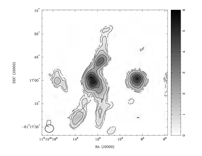
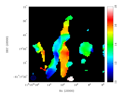
Figure 1: ATCA CS(2–1) molecular line emission in NGC 3603 MM2. Top: integrated intensity map; the contour levels are 0.25, 0.5, 1, 2, 3, 4, and 5 Jy beam^-1 km s^-1. Bottom: mean velocity field; the synthesized beam ($5.6"\times 4.9"$) is displayed at the bottom left of each panel, and the grey scale/color wedges for data values on the right of each panel.

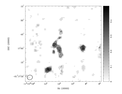
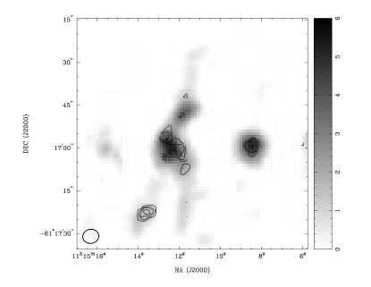
Figure 2: ATCA C³⁴S(2–1) molecular line emission in NGC 3603 MM2. Top: integrated intensity map; the contour levels are 0.16, 0.24, 0.32, and 0.40 Jy beam^-1 km s^-1. Bottom: C³⁴S(2–1) contours overlaid onto CS(2–1) emission map. The synthesized beam ($5.6"\times 4.9"$) is displayed at the bottom left of each panel, and the grey-scale wedge for data values on the right of each panel.

Figure 3: ATCA CS(2–1) spectra at four selected positions (coordinates given in the panels) within NGC 3603 MM2. From left to right and top to bottom: sources S9 , Sc , Sa , Se of Fig. 4.

2.2 SABOCA sub-mm imaging

Observations of NGC 3603 MM2 at 350 $\mu$m with the SABOCA bolometer array (Siringo et al. 2010) attached to the APEX telescope on the Chajnantor plateau in Chile were carried out on September 15, 2011, providing a beam FWHM of 7.8”. The precipitable water vapor column was about 0.2 mm during the observations which lasted about 15 minutes for a spiral raster map of about 1.5 arcminutes in radius centered on IRS 9A. For the calibration, a sky dip determined a zenith opacity of 0.736, and absolute calibration was established with observations of VY CMa and B13134 from the APEX primary and secondary calibrator list. The accuracy of the absolute calibration is estimated to be 10%. The map is shown in Fig. 4.

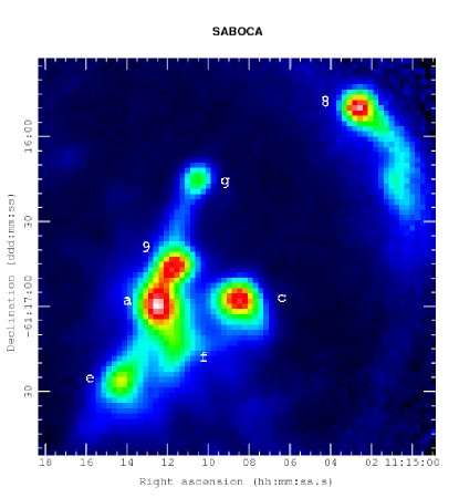
Figure 4: SABOCA 350 $\mu$m image of NGC 3603 MM2. The source labeled “9” (S9 ) is associated with IRS 9A. This source and the source labeled “c” (Sc ) were the targets for SHFI spectroscopy. The source labeled “g” (Sg ) is at the tip of the eastern pillar (see Figs. 1 of Brandl et al. (1999) and Mücke et al. (2002)), while the source labeled “8” (S8 ) is at the tip of the western pillar, both pointing towards the OB cluster. The wedge at the bottom shows the scale for the image flux densities in Jy/Beam.

Seven distinct sources can be identified in the 350 $\mu$m SABOCA image (Fig. 4), some of which were already seen in the ATCA CS maps (Figs. 1 and 2). The positions of the sources and their flux densities were extracted by iteratively fitting and subtracting two-dimensional Gaussian profiles, starting with the brightest source. The total fluxes were derived from the fitted peak flux and width of the Gaussian profiles, deconvolved from the beam width. The results are summarized in Table 2.

Table 2: Properties of SABOCA sources. The sources labeled S8 and S9 in the first column are the same as listed in Table 1 of Lebouteiller et al. (2008). Source S9 is associated with IRS 9A. The source size $\theta$ in column 5 is the geometric mean of the axes of the deconvolved size. At the distance of IRS 9A, 10” correspond to 0.33 pc. The data in the last three columns are described in Section 3.3.

	RA	Dec	$F$	$\theta$	$\Delta$v	$M_{F}$	$M_{V}$
			Jy	”	km/s	$M_{\odot}$	$M_{\odot}$
Sa	11:15:12.07	-61:16:58.8	90	9.2	2.5	498	122
S8	11:15:02.88	-61:15:51.5	55	6.7	$-$	307	0
Sc	11:15:08.41	-61:16:57.2	67	8.2	3.2	369	180
S9	11:15:11.34	-61:16:45.2	59	7.6	2.5	329	102
Se	11:15:13.73	-61:17:24.3	46	8.5	2.5	258	114
Sf	11:15:11.25	-61:17:12.0	45	9.6	$-$	249	0
Sg	11:15:10.33	-61:16:16.4	22	4.9	$-$	122	0

2.3 SHFI sub-mm spectroscopy

Table 3: SHFI observational parameters. The main beam efficiencies ($\eta_{\rm mb}=0.75$ for APEX-1 and $0.73$ for APEX-2) and conversion factors ($39$ K/Jy for APEX-1 and $41$ K/Jy for APEX-2) are taken from http://www.apex-telescope.org/telescope/efficiency/

Receiver	Setting	Range	Noise	PWV
		GHz	mK	mm
APEX-1	1	216.9 – 220.9	10	2.0
	2	229.2 – 233.2	30	2.0
APEX-2	3	346.1 – 350.1	30	1.5
	4	353.2 – 357.2	30	0.4
	5	345.8	50	0.3

Observations with the SHFI instrument (Vassilev et al. 2008) attached to APEX were carried out in 2012. The observations with the APEX Band-1 (211 - 275 GHz) receiver were carried out July 31, those with the Band-2 receiver (275 - 370 GHz) August 1 (setting 3) and October 10 (setting 4). Finally, on October 12, a 25-pointing map was executed in the CO (3-2) line (setting 5). Details are given in Table 3. For all observations, a velocity resolution of 0.5  km s^-1was chosen.

Each observation sequence (except for the map) included two back-to-back pointings towards sources S9 and Sc (28” distance), sandwiched between two observations of the sky at RA = 11:19:58.5 and DEC = -60:09:57.8 which was selected for its low 100 $\mu$m emission (IRAS) a short distance away (1.2 degrees). Even with the largest beam of 32” of APEX Band-1, the distance between S9 and Sc of 28” is large enough to prevent mutual contamination. However, sources S9 and Sa have a distance of 16” so that the flux measured at position S9 might be contaminated by emission from Sa , as half of the flux of Sa will be picked up by the 28” beam.

The spectra with a bandwidth of 4 GHz were reduced using the CLASS software. In order to identify the lines, the systemic velocity of source c was measured from the optically thin isotopologues of CO (C¹⁸O) to be +13  km s^-1. NIST recommended rest frequencies of the lines were used to identify the lines listed in Table 4, together with their properties and the antenna temperature peak ratios between sources Sc and S9 ($T_{\rm c}/T_{\rm 9}$).

We used the WEEDS extension (Maret et al. 2011) of CLASS to confirm the line identifications on source S9 by checking for each species the presence of lines in any of our wavelength settings. Using the three Formaldehyde lines we detected in setting 1, we determined an excitation temperature of 45 K as this value reproduced the measured line ratios. All lines were fit with this temperature, and a line width of 5 km/s. Two of the lines, ¹³CO and C¹⁸O, are extended by about a factor of six over the other line emitting regions, which we adopted at 5” in size (unresolved by APEX). Increasing the number density of the species instead would have led to saturation of the lines.

Two lines near 230.232 GHz and 230.841 GHz remained unidentified. The closest matches of lines from SO¹⁷O, CH₃OCH₃, and CH₂CHCN, respectively, predicted more lines of these species to be seen in setting 4, but were not detected.

The full spectra are shown in Fig. 9 and 10, while spectra of the identified lines are shown in Figs. 5 to 8. In all plots, the units are antenna temperatures in Kelvin versus km/s.

Table 4: Molecular lines (species, transition, frequency, and upper energy level $E_{u}$) identified. All lines were detected in both positions. Also the ratio of the antenna peak temperature between the offset position (source Sc ) and source S9 is given in the last column (a hyphen indicates no significant difference for very weak lines).

Species	Transition	$\nu_{0}$	$E_{u}$	$T_{\rm Sc}/T_{\rm S9}$
		(GHz)	(K)
SiO	5-4	217.104984	31.2	–
DCN	3-2	217.238531	20.9	1.32
c-HCCCH	6(1,6)-5(0,5)	217.822141	38.6	1.47
CH3OH	4(2,2)-3(1,2)	218.440047	45.5	–
H2CO	3(0,3)-2(0,2)	218.222188	21.0	1.39
…	3(2,2)-2(2,1)	218.475641	68.1	1.30
…	3(2,1)-2(2,0)	218.760078	68.1	1.41
C18O	2-1	219.5603	15.8	1.19
SO	5,6-4,5	219.949438	35.0	1.45
13CO	2-1	220.3986	15.86	0.97
CO	2-1	230.538	16.6	0.75
13CS	5-4	231.220688	33.3	–
H$\alpha$	H$30\alpha$	231.900930	Rec.	–
SO	8,9-7,8	346.528594	78.8	2.40
H13CO$+$	4-3	346.998347	41.6	3.37
H2CS	10(1,9)-9(1,8)	348.534250	105.2	–
C2H	4(7/2,4)-3(5/2,3)	349.399342	41.9	2.88
…	4(9/2,4)-3(7/2,3)	349.339067	41.9	2.5
H$\alpha$	H$26\alpha$	353.622747	Rec.	–
HCN	4-3	354.505469	42.5	1.80
HCO$+$	4-3	356.734250	42.8	1.62

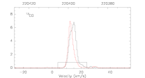
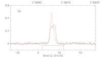
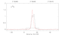
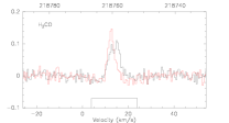
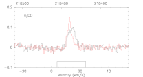
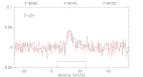
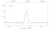
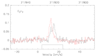
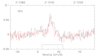
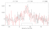
Figure 5: APEX SHFI spectra (setting 1) of source S9 (black) and source Sc (red) in antenna temperature (Kelvin) versus km/s. The beam FWHM is 32”. All spectra smoothed with 5-channel box. The rectangles indicate data excluded from the baseline fit.

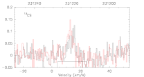
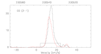
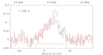
Figure 6: APEX SHFI spectra (setting 2) of source S9 (black) and source Sc (red) in Kelvin versus km/s. The beam FWHM is 29”. All spectra smoothed with 5-channel box, 10-channel box for H$30\alpha$.

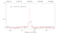
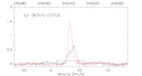
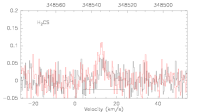
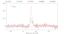
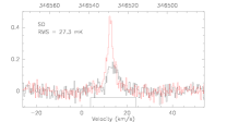
Figure 7: APEX SHFI spectra (setting 3) of source S9 (black) and source Sc (red) in Kelvin versus km/s. The beam FWHM is 20”. All spectra smoothed with 5-channel box.

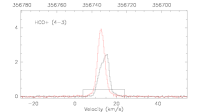
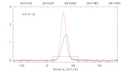
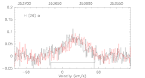
Figure 8: APEX SHFI spectra (setting 4) of source S9 (black) and source Sc (red) in Kelvin versus km/s. The beam FWHM is 19”. All spectra smoothed with 5-channel box, 10-channel box for H$26\alpha$.

Figure 9: Full-bandwidth spectra for settings 1 and 2 recorded with SHFI on source Sa . All spectra were smoothed with a 10-channel box. The “wiggles” of the baseline in the lower left panel are due to instrumental problems. Dotted lines mark frequencies of molecular lines which we expected to see, but didn’t.

Figure 10: Full-bandwidth spectra for settings 3 and 4 recorded with SHFI on source Sa . All spectra were smoothed with a 10-channel box. The “wiggles” of the baseline in the lower left panel are due to instrumental problems. Dotted lines mark frequencies of molecular lines which we expected to see, but didn’t.

3 Results

3.1 Cores and filaments

We resolved the molecular cloud clump MM2 into numerous sources (“compact cores”) both in the CS(2–1) line and sub-mm continuum emission. There is a clear correspondence of the compact cores seen at mm-wavelength to their counterparts seen in the sub-mm. The emission has the general appearance of clumpy filaments.

The CS(2–1) line emission in NGC 3603 MM2 ranges from at least 10 to 20 km s^-1. The mean CS(2-1) velocity field shows basically two filaments a few  km s^-1apart, which was seen in CS spectra already by Nürnberger et al. (2002). One extends from source Sg over S9 , Sa , and Sf at a systemic velocity of 15 –16  km s^-1(see Fig. 1), while the other one extends from source S9 over Sa to Se at a systemic velocity of about 12  km s^-1. As the two filaments overlap at the position of source S9 , the line profiles are double-peaked here, also indicating optically thin emission.

We observed the optically thin/thick pair of lines H¹³CO$+$/HCO$+$ (Figs. 7/8) which can be used to trace infall (Myers et al. 1996; Klaassen & Wilson 2007; Chen et al. 2010) if the optically thick line of HCO$+$ is double peaked, with a stronger blue peak. The optically thin line of H¹³CO$+$ is used to rule out possible self-absorption (the line would have a single peak at the frequency of the absorption). Instead, we see that the H¹³CO$+$ line is double peaked itself, and thus the line shapes do not indicate infall, but are again the result of superposed filaments at different LSR velocities.

Weak C³⁴S(2–1) emission from several of the compact cores was detected as well (see Fig. 2) and appears to wrap around the peak of the CS(2–1) emission of the strongest source Sa (see Fig. 4 for the source nomenclature), a behaviour also found by Beuther et al. (2009) from observations towards massive warm molecular cores. The same is true for very weak emission peak at the position of component S9 , while the C³⁴S(2–1) emission is peaked at the positions of sources Sc and Se . Similar offsets were observed by Immer et al. (2014) in W33 Main (their Fig. A.6), but no explanations for the offsets were given.

3.2 Temperature of the compact cores

Following Mangum & Wootten (1993), the gas temperature can be determined from the peak flux ratio of selected formaldehyde (H₂CO) lines. In particular, for two of the lines we detected ($3_{03}-2_{02}$/$3_{22}-2_{21}$), Fig. 13b of Mangum & Wootten (1993) indicates a range of temperatures (depending on the number density of molecular Hydrogen ranging from $10^{4}$ to $10^{5}$ per cm³) between 50 K and 60 K given a ratio of 5 for the peak flux ratio. The lower value of this range is consistent with the temperature we fit (45 K) to the formaldehyde line ratios using WEEDS (and for source Sa as well). A similar gas temperature (47 K) has been determined for MM2 by Röllig et al. (2011), while a dust temperature of 47 K for the MM2 pillar has been derived from SED fitting by Di Cecco et al. (2015).

3.3 Mass of the compact cores

We computed the total gas and dust mass, $M_{F}$, of the cores based on their 350 $\mu$m flux using equation D6 of Galván-Madrid et al. (2013) with an absorption coefficient of $\kappa_{\rm 850GHz}=5.9$ cm²/g (Table 1, column 5 of Ossenkopf & Henning 1994), giving, for example, a mass of 250 to 330 M_⊙ for source S9 for the range of temperatures given above. The results are listed in Table 2 (column 7) for all compact cores, assuming they have all the same temperature of 50 K. The total mass of all compact cores in MM2 (therefore not including source S8 ) is about 1800 $M_{\odot}$ and therefore appears to be consistent with the mass estimate of 1500 solar masses for MM2 by Nürnberger et al. (2002). Adopting a value of $\kappa_{\rm 100GHz}=0.2$ cm²/g from an extrapolation using the data of Ossenkopf & Henning (1994) to the wavelength of the ATCA observations, the continuum RMS of 35 mJy/beam corresponds to more than 200 M_⊙ and thus explains why the cores were not detected in continuum emission with ATCA.

We also computed, using the prescription of MacLaren et al. (1988), the virial masses, $M_{V}$, of the four sources in Fig. 3 for which we can measure the CS line widths. In the cases of a double-peaked line profile (sources S9 and Sa ), which are due to a superposition of two filaments, we decomposed the profile into two and used the width of the line component at the lower velocity (as they correspond better to the velocity of the other two sources). In these cases, the virial masses would be underestimated and are indeed only about 30% of the flux-based masses, while the virial masses of the sources Sc and Se are about 50% of the flux-based estimates. These results are also listed in Table 2.

3.4 Extended CO gas emission and outflow

In Fig. 11 we show spectra of the CO(3–2) line at 25 positions forming a raster across MM2. The decrease in line strength at positions West of source S9 is consistent with there being no CO emission (the beam FWHM is 20”). This is not the case in directions North and East, indicating the presence of extended CO emission here.

Towards the South-East, a shoulder emerges in the line redshifted by a few  km s^-1. Comparing this location with the mean CS(2–1) velocity field in Fig. 1, we conclude that the shoulder is due to the filament associated with source Sa which has a line of sight (LOS) velocity of about 16  km s^-1, while source S9 has a LOS velocity of about 12  km s^-1.

The CO (2-1) line shown in Fig. 6 shows more emission peaks at velocities of +25 – 30 km/s (amplitudes of 2 K). These can also be seen in Fig. 11. Since they are separated from the LSR velocity by more than the redshifted filament could explain, we interpret this as a hint towards a high velocity outflow. Further evidence for an outflow comes from our detection of the (very weak) SiO line (Fig.5), which is generally interpreted as an outflow tracer (e.g. Klaassen & Wilson 2007). Despite it’s low SNR, the shape of this line appears to be triangular, indicating the existence of line wings.

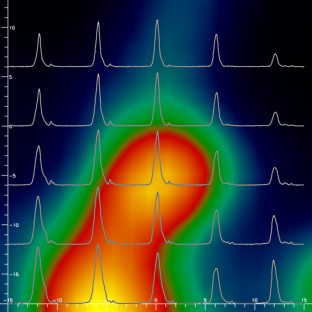
Figure 11: APEX CO(3–2) (345 GHz) spectra in a grid of 25 positions (6” spacing) in a region of MM2 centered on IRS 9A (source S9 ). North is up and East to the left, and coordinates are in arc-seconds relative to Sa . The individual spectra, each covering 60 km/s, are displayed over the SABOCA map, with the center and base of every line aligned with the corresponding pointing position. The maximum line peak is 28 K main beam temperature. The beam FWHM is 20”.

3.5 Radio-recombination lines

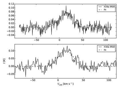
Figure 12: APEX hydrogen recombination lines H$26\alpha$ and H$30\alpha$ with Gaussian fits.

Figure 12 shows the millimeter hydrogen recombination line (RL) emission towards the center of IRS 9. The detection of these lines demonstrates the effect of photoionization feedback from the central massive star(s) in IRS 9. The RL emission appears to be extended, since the line is also detected away from IRS 9. High angular resolution RL mapping is needed to determine the nature of the RL emission, whether diffuse (e.g., Garay et al. 1998), or an ultracompact or hypercompact H ii region (Hoare et al. 2007).

The FWHMs of the H$26\alpha$ and H$30\alpha$ lines are the same within uncertainties (FWHM${}_{\mathrm{H26}}=34.8\pm 1.8$ km s^-1, FWHM${}_{\mathrm{H30}}=33.5\pm 2.0$ km s^-1). This is consistent with previous observations in other regions which show that mm RLs are free from collisional broadening compared to cm RLs (e.g. Keto et al. 2008; Galván-Madrid et al. 2012). Therefore, the observed line width can be explained as a combination of the thermal width of ionized gas at $10^{4}$ K ($\sim 20$ km s^-1) and dynamical broadening due to bulk motions of order $2c_{s}$, where $c_{s}\sim 10$ km s^-1 is the speed of sound of the ionized gas. The centroid LSR velocities of both lines are also the same within uncertainties, and consistent with the IRS 9 systemic velocity as derived from dense molecular gas: $V_{\mathrm{LSR,H26}}=14.4\pm 0.8$ km s^-1, $V_{\mathrm{LSR,H30}}=15.8\pm 0.9$ km s^-1. Finally, we note that the velocity-integrated line intensities for both lines are about the same. For resolved observations, and assuming LTE and low line and free-free continuum optical depths, the line ratio should scale approximately linearly with frequency (e.g. Keto et al. 2008; Galván-Madrid et al. 2012). Two possible explanations for our observations are that: the H$26\alpha$ line, because its lower optical depth, has a smaller filling factor within the APEX beam than the H$30\alpha$ line; or that the H$30\alpha$ line is amplified due to non-LTE effects (e.g. Jiménez-Serra et al. 2013). Sub-arcsecond angular resolution RL observations are necessary to test these hypotheses.

4 Discussion

The most obvious feature of our sub-mm spectra of sources S9 and Sa is the lack of lines typically seen in hot-cores (e.g. Olmi et al. 1993), especially the series of lines of Methylcyanide, Methanol, and OCS in the 217 – 221 GHz band (see upper left panel of Fig. 9).

A prominent feature instead is the presence two Ethynyl lines near 349 GHz. According to Beuther et al. (2008), these lines are seen in all evolutionary stages of massive stars beginning with infrared dark clouds (IRDCs), and continuing via high-mass protostellar objects (HMPOs) to ultracompact H ii regions (UCHII). When comparing our full spectrum for setting 3 (Fig. 9) to Fig. 1 of Beuther et al. (2008), it is obvious that source S9 is not a HMPO. The mean Ethynyl line widths are 3.0  km s^-1for the two earlier evolutionary stages, while they are 5.5  km s^-1for the UCHIIs. On source Sc , we measured a line width of 3.3  km s^-1, and on S9 6.0  km s^-1. However, the latter is clearly a superposition of two line profiles originating in different filaments, and fitting double-Gaussian profiles yield an average width of $3.1\pm 0.4$ km/s. Therefore, we would classify these compact cores as IRDCs even though their temperature is about twice that one would expect for IRDCs (Pillai et al. 2006). As shown in Fig. 14, none of the compact cores shows free-free emission at 5 GHz, thus do not appear to harbor UCHII regions.

If we look at the MIR emission in the region around IRS 9A (Nürnberger & Stanke 2003)) and overlay the contours of the 350 $\mu$m map we obtained with SABOCA (Fig. 13), we see that sources Sc , Sg (tip of the eastern pillar), and S8 seem opaque to background MIR emission, consistent with a classification of IRDCs. IRS 9A itself is quite close to source S9 , but apparently in front of it. (The MIR position of Nürnberger (2003) is about 3.6” away from the position of S9 , even though more recent astrometric analysis by Brandner (priv. comm.) reduces the offset to 1.8”.) Similarly, extended MIR emission seen towards Sa must originate in the forground while still associated with warm dust in the region. It thus appears that IRS 9A may have been formed more recently than the OB cluster stars out of a compact core like the ones we found in MM2.

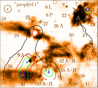
Figure 13: TIMMI2 11.9 $\mu$m image (Fig. 4c of Nürnberger & Stanke 2003) with overlaid contours of the SABOCA map. The image size is 95” by 110”. The labeling is from Nürnberger & Stanke (2003) and denotes the position of the cluster with an open circle, the positions of IR sources from Frogel et al. (1977) with asterisks, while all other labels refer to sources given by Nürnberger & Stanke (2003). The photo-center of the SABOCA source closest to IRS 9A is shifted by about 3” to the East-South-East. Component S8 of the SABOCA image coincides quite well with a maser source indicated by the square, according to Nürnberger & Stanke (2003).

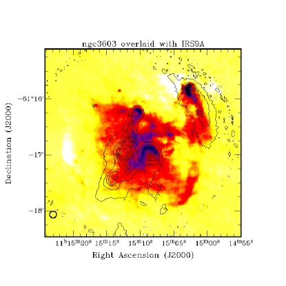
Figure 14: Overlay of SABOCA contours on a 5 GHz image of the H ii region obtained from ATCA data by Mücke et al. (2002). The blue colored image regions correspond to the largest 5 GHz fluxes, while the yellow color denotes the faintest 5 GHz emission. The contour levels are at 87%, 73%, 60%, 46%, 33%, 19%, and 06% of the maximum. The ATCA beam is 2”, the SABOCA beam is 7.8” and is shown in the lower left corner.

Evidence for ionized gas around IRS 9A has been found from Spitzer spectra, showing lines of [Ne II] and [S IV] (Lebouteiller et al. 2008). Similarly, Röllig et al. (2011) reached the conclusion that “the cluster is strongly interacting with the ambient molecular cloud” based on their map of the FUV radiation field. Both Figs. 14 and 15 illustrate this by showing strong free-free emission at 6 cm and H$\alpha$ recombination line emission in the NGC 3603 region at the head of the eastern (source Sg ) and western (source S8 ) pillar, as well at the circumference of source Sc facing the cluster. These regions likely contribute to the RL emission we detected.

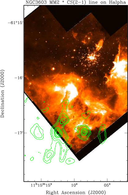
Figure 15: ATCA CS (2–1) contour overlay on an HST H-$\alpha$ image (Brandner et al. 2000).

The fact that compact cores make up the clump MM2 and the close association of the IR source 9A to one of them (source S9 ) may fit into the picture of sequential star formation from the north to the south (de Pree et al. 1999), away from the OB cluster which itself is possibly the result of a cloud-cloud collision (Fukui et al. 2014). Not far from IRS 9A, Roman-Lopes (2013) identified MTT 58 (Melnick et al. 1989) as an O2 star very close (in projection) to the molecular cloud core MM2E (source Sc ) seen first by Nürnberger et al. (2002) in C¹⁸O (2–1) data, indicating that this star, like IRS 9A, might still be embedded in a parental gas and dust. Roman-Lopes (2013) estimated the age of this star to be no more than 600 000 years, based on the size of the associated H ii region. The age of the central star of IRS 9A is about 70 000 years in the model 3012790 of Robitaille et al. (2006) which was fit by Vehoff et al. (2010) to the spectral energy distribution of IRS 9A.

5 Conclusions

The SABOCA $350\mu$m image of the bright infrared source IRS 9A in the nearby H ii region NGC 3603 confirms the presence of multiple massive cores in the molecular clump MM2, while the SHFI spectra do not show the typical hot core lines such as those from Methylcyanide. Based on their mid-infrared opacity, we classify these cores as infrared dark clouds even though their temperature of about 50 K is higher than expected for IRDCs. The mid-IR source IRS 9A is associated with a massive core, but outside it, and could be in a stage just after ”hot core”, i.e. an ultra-compact H ii region, ionized by a massive star in its center. Millimeter hydrogen recombination line emission was detected in this direction, but also from a nearby core indicating a potentional diffuse contribution due to the ionizing radiation from the cluster. It is the only source in MM2 strong in the mid-infrared. The structure of MM2 as seen in the CS(2–1) line at $3$ mm by ATCA is characterized by filaments at different systemic velocities. The CO mapping data do not show conclusive evidence for a high velocity outflow, certainly not for a very massive one. However, the presence of SiO emission, with a hint of line wing emission, is indicative of weak outflow activity.